applied machine learning for systematic equities trading

1

Applied Machine Learning For Systematic Equities Trading:

Trend Detection, Portfolio Construction and Order Execution

Mininder Sethi

A dissertation submitted in partial fulfilment

of the requirements for the degree of

Doctor of Philosophy

of

University College London

Department of Computer Science

University College London (UCL)

2016

2

Declaration

I, Mininder Sethi, declare that this Thesis is my own work. Where information has been derived from

other sources, such sources have been properly referenced.

3

Abstract

The systematic trading of equities forms the basis of the Global Asset Management Industry. Analysts

are all trying to outperform a passive investment in an Equity Index. However, statistics have shown

that most active analysts fail to consistently beat the index. This Thesis investigates the application of

Machine Learning techniques, including Neural Networks and Graphical Models, to the systematic

trading of equities. Through approaches that are based upon economic tractability it is shown how

Machine Learning can be applied to achieve the outperformance of Equity Indices.

In this Thesis three facets of a complete trading strategy are considered, these are Trend Detection,

Portfolio Construction and Order Entry Timing. These three facets are considered in an integrated

Machine Learning framework and a number of novel contributions are made to the state of the art. A

number of practical issues that are often overlooked in the literature are also addressed. This Thesis

presents a complete Machine Learning based trading strategy that is shown to generate profits under a

range of trading conditions. The research that is presented comprises three experiments:

1- A New Neural Network Framework For Profitable Long-Short Equity Trading - The

first experiment focusses on finding short term trading opportunities at the level of an

individual single stock. A novel Neural Network method for detecting trading opportunities

based on betting with or against a recent short term trend is presented. The approach taken is

a departure from the bulk of the literature where the focus is on next day direction prediction.

2- A New Graphical Model Framework For Dynamic Equity Portfolio Construction - The

second experiment considers the issue of Portfolio Construction. A Graphical Model

framework for Portfolio Construction under conditions where trades are only held for short

periods of time is presented. The work is important as standard Portfolio Construction

techniques are not well suited to highly dynamic Portfolios.

3- A Study Of The Application of Online Learning For Order Entry Timing - The third

experiment considers the issue of Order Execution and how to optimally time the entry of

trading orders into the market. The experiment demonstrates how Online Learning techniques

could be used to determine more optimal timing for Market Order entry. This work is

important as order timing for Trade Execution has not been widely studied in the literature.

The approaches that form the current state of the art in each of the three areas of Trading Opportunity

(Trend) Detection, Portfolio Construction and Order Entry Timing often overlook real issues such as

Liquidity and Transaction Costs. Each of the novel methods presented in this Thesis considers such

relevant practical issues.

4

This Thesis makes the following Contributions to Science:

1- A novel Neural Network based method for detecting short term trading opportunities for

single stocks. The approach is based upon sound economic premises and is akin to the

approach taken by an expert human trader where stock trends are identified and a decision is

made to follow that trend or to trade against it.

2- A novel Graphical Model based method for Portfolio Construction. Standard Portfolio

techniques are not well suited to a dynamic environment in which trades are only held for

short time periods, a method for Portfolio Construction under such conditions is presented.

3- A study of the application of Online Learning for Order Entry Timing. Order Entry Timing

for Trade Execution has not been widely studied in the literature. It is commonly assumed

that trading orders would be executed at the day end closing price. In practice there is no real

reason to trade on the close and it is shown that better execution may be obtained by trading

at an earlier time which can be determined through the application of Online Learning.

5

Summary of Publications

This Thesis builds upon ten years of work experience in the Financial Services Industry as both a

Quantitative Analyst and as a Trader. The motivation was to conduct a substantial piece of original

research which could find application in the Financial Services Industry. At the same time there was a

desire to create something with a solid Academic Basis that could be published into the Academic

Literature and that adds to the current published State of the Art. The content of this Thesis has

formed the basis of three publications that appear in the proceedings of world renowned conferences

in the fields of Computer Science and Neural Networks. These publications are

[Publicaton-1] Sethi, M; Treleaven, P; Del Bano Rollin, S (2014). "A New Neural Network

Framework for Profitable Long-Short Equity Trading". Proceedings of the 2014 IEEE

International Conference on Computatonal Science and Computational Intelligence (CSCI

2014). Vol. 1. Pages 472-475.

[Publicaton-2] Sethi, M; Treleaven, P; Del Bano Rollin, S (2014). "Beating the S&P 500 Index -

A Successful Neural Network Approach". Proceedings of the 2014 IEEE Joint International

Conference on Neural Networks (IJCNN 2014). Vol. 1. Pages 3074-3077.

[Publicaton-3] Sethi, M; Treleaven, P (2015). "A Graphical Model Framework for Stock Portfolio

Construction with Application to a Neural Network Based Trading Strategy". Proceedings of the

2015 IEEE Joint International Conference on Neural Networks (IJCNN 2015). Vol. 1. Pages 1-8.

These publications represent a subset of the original academic contributions of this Thesis with

there being room for further publications. Details of such further possible publications are given

in Chapter 7 of this Thesis.

6

Acknowledgements

After gaining ten years of work experience in the Financial Services Industry as both a Quantitative

Analyst and as a Trader I was convinced that there were smarter ways of doing things and that there

was room to embrace Data and Machine Learning. I would like to firstly acknowledge those people

that shared in this vision, my Principle Supervisor Professor Philip Treleaven and both of my Second

Supervisors Dr Sebastian Del Bano Rollin and Mr Donald Lawrence. I appreciate the guidance and

motivation that my Supervising Team provided me throughout this period of research.

I would also like to thank the general faculty and research students within the UK Financial

Computing Centre at University College London for their support, encouragement and friendship. The

Centre provided a highly conducive environment in which to conduct research and being part of a

group of such talented people with such diverse backgrounds has been a truly pleasurable experience.

I dedicate this Thesis to my lovely wife Jinhwa Kim without whose support I would have been unable

to undertake this project.

7

Contents

1 Introduction 12

1.1 Motivation for This Thesis: Markets Are Predictable 12

1.2 Research Objectives 15

1.3 Thesis Subject Matter 16

1.4 Major Contributions 16

1.5 Thesis Outline 17

2 Background 19

2.1 An Overview of Machine Learning 19

2.1.1 Regression and Classification: Neural Networks and Support Vector

Machines 19

2.1.2 Probabilistic Modelling: Graphical Models and Graph Theory 24

2.1.3 Online Learning 27

2.2 An Overview of a Complete Trading Strategy 30

2.3 Trading Opportunity Detection 31

2.3.1 Overview of Trading Opportunity Detection 31

2.3.2 Machine Learning for Trading Opportunity Detection 36

2.4 Portfolio Construction 44

2.5 Order Entry Timing: Market Order Book and Order Execution 51

2.6 Summary 55

3 A New Neural Network Framework For Profitable Long-Short Equity Trading 56

3.1 Introduction 56

3.2 A Novel Method for Trend Detection Without Machine Learning 57

3.3 First Neural Network Approach for Trend Detection 66

3.4 Improved Neural Network Approach for Trend Detection 71

3.5 Optimising Neural Network Trend Detection 76

3.6 Testing the Proposed Method 81

3.7 Summary 83

4 A New Graphical Model Framework For Dynamic Equity Portfolio Construction 85

4.1 Introduction 85

4.2 Simple Approach to Portfolio Construction, Beating the Index 87

4.3 Application of Current Portfolio Methods, Room For Improvement 88

4.4 A Novel Method for Portfolio Construction 95

4.5 Improving the Method with Chain Optimisation 104

4.6 Testing the Proposed Method 107

4.7 Summary 110

5 A Study Of The Application Of Online Learning For Order Entry Timing 111

5.1 Introduction 111

5.2 Framework for the Order Execution Problem 112

5.3 Online Learning Approaches for Order Execution 116

8

5.4 Testing the Proposed Methods 130

5.5 Summary 135

6 Assessment 136


6.2 Assessment Of A New Neural Network Method For Profitable Long Short

Equity Trading 137

6.3 Assessment Of A New Graphical Model Framework For Dynamic Equity

Portfolio Construction 139

6.4 Assessment Of A Study Of The Application Of Online Learning For Order

Entry Timing 141

7 Publications, Future Work and Conclusions 143


7.2 Overview of Published Work 144

7.3 Proposals for Further Publications and Future Research 145

7.4 Conclusions 146

References 147

9

List of Figures

2.1 An Example Feedforward Artificial Neural Network (ANN) Architecture 21

2.2 An Illustration of Separating Hyperplanes in a 𝑑 = 2 Dimension Feature Space 23

2.3 An Example Bayesian Network with 𝑑 = 4 Random Variables 25

2.4 An Example Markov Network with 𝑑 = 4 States 26

2.5 A Complete Trading Strategy and its Building Blocks 31

2.6 Rolling 260 Business Day Historical Return for Two Example Stocks 47

2.7 Rolling 260 Business Day Realized Volatility for Two Example Stocks 48

2.8 Rolling 260 Business Day Realized Correlation for Two Example Stocks 48

2.9 Percentage of Portfolio Invested into One Stock with Mean-Variance Optimization 48

2.10 Example Double Auction Based Limit Order Book for General Electric 51

2.11 Example Double Auction Based Limit Order Book for Cimarex Energy 52

3.1 Illustrative Period of Low Short Term Efficiency (𝛾𝑀𝐶𝐷 = 0.05, with 𝐾 = 10) 58

3.2 Illustrative Period of High Short Term Efficiency (𝛾𝑀𝐶𝐷 = 1.00, with 𝐾 = 10) 59

3.3 Historical Conditions for Anomalies for JPM between April 03 and April 10 62

3.4 Historical Conditions for Anomalies for UNH between April 03 and April 10 63

3.5 Historical Conditions for Anomalies for XOM between April 03 and April 10 63

3.6 Historical Conditions for Anomalies for JNJ between April 03 and April 10 63

3.7 A Training Set for MCD Generated for May 09 to May 12 68

3.8 Output of the RBFNN Trained Using the Data in Figure 3.7 68

3.9 Re-Categorised Training Set for MCD Generated for May 09 to May 12 73

3.10 Output of the RBFNN After Training Using Re-Categorised Training Data 73

3.11 Zero Appended Neural Network Training Set for MCD 74

3.12 Output of the RBFNN After Training Using the Zero Appended Data 74

3.13 Mapping to Proposed Cost Function 78

3.14 Optimized Values of the Short Term Efficiency Level Exit Threshold 𝛿𝑇𝐶𝐾 80

3.15 Optimized Values of the Trade Categorisation Threshold 𝜔𝑇𝐶𝐾 80

4.1 CDF of Number of Buy Trades Generated per Day for a First Sample of 100 Stocks 86

4.2 CDF of Number of Sell Trades Generated per Day for a First Sample of 100 Stocks 86

4.3 Portfolio Levels Against Benchmarks for a First Sample of 100 Stocks 87

4.4 Portfolio Levels Against Benchmarks for a Second Sample of 100 Stocks 88

4.5 QQ-Plot of 1 Day Returns for Long Trades Generated Across 100 Stocks 90

4.6 QQ-Plot of 1 Day Returns for All Returns Generated Across 100 Stocks 91

4.7 Rolling Annualised One Business Day Historical Return for Example Stocks 91

4.8 Rolling Annualised Volatility for Example Stocks 92

4.9 Rolling 260 Business Day Realized Correlation for Two Example Stocks 92

4.10 Percentage Allocation to Example Stocks Based on Sharpe Ratio Optimization 92

4.11 Rolling Annualised In-Situ One Business Day Returns for Example Stocks 93

4.12 Rolling Annualised In-Situ Volatility for Example Stocks 94

4.13 Rolling In-Situ Realized Correlation for Two Example Stocks 94

4.14 Percentage Allocation to Example Stocks Based on Sharpe Ratio Optimization 94

4.15 A Simplified Model of the Internet with Just 4 Web Pages 95

4.16 A Complete Markov Chain Model for Portfolio Construction with 4 Stocks 98

4.17 A Simplified Markov Chain Model for Portfolio Construction with 4 Stocks 99

10

4.18 Evolving Distributions for Two Example Stocks 101

4.19 Convergence of the Distribution of Funds Amongst 5 Stocks and Bridge Portfolios 103

4.20 Convergence of the Distribution of Funds after Bridge Portfolio Reallocation 104

4.21 Percentage Allocation to Two Example Stocks Based on Proposed Method 104

4.22 An Example Graphical Model Ordering 105

4.23 An Alternative Graphical Model Ordering 105

4.24 Convergence of Proposed GA Method for a Universe of 20 Stocks 106

4.25 Convergence of Proposed GA Method for a Universe of 99 Stocks 107

4.26 Empirical CDF of MC Simulation Results for Sub-Universes of 100 Stocks 108




5.1 Evolution of the Best Bid Price for Verizon 112

5.2 Best Bid Price Predictions Based on a Simple Moving Average Predictor 114

5.3 Sample Prediction Errors for Two Expert Predictors 117

5.4 Sample Predictions for an Online Learning Predictor 119

5.5 Sample Prediction Errors for an Online Learning Predictor 119

5.6 Profitable and Loss Making Trades for an Online Learning Predictor 120

5.7 Profitable and Loss Making Trades for an Online Learning Predictor (Long Path) 121

5.8 Expert Selection Decisions of the First Proposed Online Learning Predictor 124

5.9 Profit or Loss of the Decisions of the First Proposed Online Learning Predictor 124

5.10 Average Percentage of Profitable Trades for the Window Length 𝐿 132

5.11 Average Percentage for Which Expert-D is Chosen for the Window Length 𝐿 132

5.12 Average Percentage of Profitable Trades for the Factor 𝛽 133

5.13 Average Percentage for Which Expert-D is Chosen for the Factor 𝛽 133

5.14 Distribution of the Percentage of Time for Which Expert-D is Chosen 𝛽 = 1.10 134

11

List of Tables

3.1 Application of an Introductory Framework to Large Market Capitalisation Stocks 65

3.2 Proposed Trade Categorisation Scheme for a First Application of a Neural Network 66

3.3 Parameters for McDonalds Used to Create Training Samples Depicted in Figure 3.7 67

3.4 Average Performance Figures for a First Application of a Neural Network 70

3.5 Proposed Trade Categorisation Scheme for a Second Application of a Neural Network 71

3.6 Parameters for McDonalds Used to Create Training Samples Depicted in Figure 3.9 73

3.7 Average Performance Figures for a Second Application of a Neural Network 75

3.8 Summary of Parameters that are Open to Optimisation 76

3.9 Optimized Values for Parameters Based on Average of the Cost Function 79

3.10 Average Performance Figures for an Optimized Neural Network Framework 82

3.11 Average Performance Figures for a Second Set of Stocks 83

4.1 Number of Trades Generated for a Subset of Stock Pairs over a Six Year Period 89

4.2 Average Terminal Values for Different Sub-Universe Sizes 109

5.1 Application of an Online Learning Framework to Sample Stocks 122

5.2 Application of Countering an Online Learning Framework to Sample Stocks 122

5.3 Application of a First Proposed Online Learning Framework to Sample Stocks 125

5.4 Application of a Second Proposed Online Learning Framework 𝐿 = 1 126



5.7 Application of a Third Proposed Online Learning Framework 𝛽 = 1.10 129



12

Chapter 1

Introduction

The objective of this Chapter is to give an overview of this Thesis. In the first section the motivations

for the Thesis are illustrated through a discussion of the Efficient Markets Hypothesis. In the second

section an overview of the research objectives of this Thesis is presented, this is followed by a

discussion of the Thesis subject matter in the third section. A discussion of the original contributions

of this Thesis is presented in the fourth section: these are in summary, a novel method for single stock

Trend Detection, a novel method for Portfolio Construction and a study of the application of Online

Learning techniques for order entry timing. In the final section a Chapter by Chapter outline

summary of the Thesis is presented.

1.1 Motivation for This Thesis: Markets Are Predictable

This section concludes that markets are not completely efficient and are therefore potentially

predictable. This conclusion is important as it forms the motivation for this Thesis. The conclusion is

reasoned through an overview of common approaches to stock selection and through a discussion of

the Efficient Markets Hypothesis (EMH).

The global asset management industry exceeded 74 Trillion U.S. Dollars (USD) of assets under

management in 2014 [1], an 8% growth over the figure from 2013. Assets under management are

expected to continue to grow as the global population increases and new markets are opened to

investment. A significant portion of assets under management are invested into Equity Markets. As a

representative example, the market capitalisation of the 500 stocks of the Standard and Poors 500

Index (Bloomberg Code: SPX INDEX) alone accounted for around 19 Trillion USD of value as of

December 2015 [2]. Approaches to stock selection for a Portfolio can be broken down into two main

categories, Fundamental Analysis and Technical Analysis.

The Fundamental Analysis approach [3,4] looks at the Microeconomic structure of a company and at

the company’s competitive business environment to make a decision as to whether the stock price of

the company is too high or too low. Fundamental Analysis may also incorporate a review of past and

present Macroeconomic data and may also encompass a view of domestic and international

government policy. Information is generally classified as either public information or private

information, the former category encompassing information that is considered to be sufficiently

widely disseminated to be generally accessible. Whilst much of the data required for Fundamental

Analysis may be quantified, for example stock specific data such as Price to Earnings (PE) Ratios and

13

Macroeconomic data such as past period Gross Domestic Product (GDP), other data is dependent on

the subjective judgements of human analysts.

The field of Technical Analysis [5,6] focusses on the prediction of the movements of security prices

by searching for patterns in historical price charts and traded volume data. Technical Analysis covers

a wide range of methods which consider different time frames. At one extreme is the so called ‘High

Frequency Trading’ [7] which looks for very short term dislocations in an asset price or order book, a

trade may be held for only a fraction of a second. At the other extreme are methods such as the

Kondratieff Wave [8] which advocates that economies, and therefore markets for certain assets, move

through alternating fast and slow growth phases with a complete cycle lasting between 50 to 60 years.

To imply that either Fundamental Analysis or Technical Analysis would allow the formation of a

stock Portfolio which would consistently outperform an ‘Average’ or Market Portfolio is to imply that

markets are predictable. However, the starting point of much of the literature in the field of

Quantitative Finance, including the Nobel Prize winning Black-Scholes Equation [9] for pricing

European Options, is that markets are efficient and are not predictable. The Efficient Markets

Hypothesis (EMH) postulated by Eugene Fama [10] specifies three levels of Market Efficiency:

Weak Form Market Efficiency – The current stock price reflects all information contained in

historical price and volume data. All information is reflected fully, rationally and instantaneously. As

such an active investment strategy based on Technical Analysis should not earn positive risk adjusted

returns consistently and investors should therefore use a passive strategy, such as an investment into

an Index Tracker. For example an investor who would want exposure to stocks that are listed in the

USA should invest into a tracker of an index such as the Standard and Poors 500 Index (Bloomberg

Code: SPX INDEX) rather than trying to create an individual Portfolio.

Semi-Strong Market Efficiency – The current stock price not only reflects all historical price and

volume data, but in addition the price reflects all publically available information (including news

reports, analyst reports and company reports). Only unexpected information should elicit a stock price

movement. As such a stock Portfolio constructed through the application of Fundamental Analysis

methods should not be expected to outperform a Market Portfolio.

Strong Market Efficiency – The current stock price not only reflects all historic price and volume

data, but in addition the price reflects all publically and privately held information. As such no

investors, including those with inside information, should be able to outperform a Market Portfolio.

The Market Portfolio is commonly defined [11] as a Portfolio that consists of a market capitalisation

weighted sum of every asset in the market. This textbook Market Portfolio would contain all assets

including stocks and bonds, as well as more unusual assets such as antique artwork and collectable

14

toys. In practice when discussing stock Portfolios the Market Portfolio is often taken to be a relevant

Stock Index, for example the Standard and Poors 500 Index (Bloomberg Code: SPX INDEX) could

be taken as a representative Market Portfolio for stocks listed in the USA.

The EMH does not require that the stock price at any point in time is the ‘correct equilibrium price’,

only that any deviations from the equilibrium price are random and unbiased. In summary the EMH

would tell us that any future price movements of a stock should be unpredictable. In addition, as new

information becomes available to market participants the stock price would immediately change to

reflect that information. If the EMH were to be believed active stock selection would be a futile

exercise and each investor should simply hold a Market Portfolio. Although some research [12,13]

has supported the EMH, the general consensus amongst finance practitioners is that the EMH does not

hold true and more recent research [14,15,16] has supported this conclusion.

Whilst the EMH is considered to hold true ‘on average’, at any time it may be the case that some

stocks are undervalued and others are overvalued, however on average stocks should be considered

fairly priced. At any time, for a given stock, an anomaly may cause a deviation from the EMH. Some

research has suggested that such anomalies are not violations of market efficiency but are due to the

research methods employed to find such anomalies. Other research has identified more consistent

anomalies in time-series data. Examples of consistently identified anomalies include calendar

anomalies such as the January Effect [17,18], where it has been shown that some stocks outperform at

the beginning of January. Other commonly identified anomalies are Overreaction Anomalies [19,20]

where periods of strong trend are followed by a subsequent trend reversal and Momentum Anomalies

[21,22] where periods of strong trend are followed by the continuation of such a trend. Research then

suggests that trading opportunities can be found by the identification of Overpriced and Underpriced

stocks or alternatively by the identification of Overreaction and Momentum Anomalies that are

causing deviations from the EMH. However, on average stocks should be considered fairly priced.

So at this stage it appears that the EMH, whilst being a convenient starting point for much work in the

area of Quantitative Finance, has been shown to only hold on average. This then presents a

justification for active analysis. However, research [23] has shown that in the period from 2010 to

2015 the vast majority of US Stock Funds based on Active Management had failed to beat the broad

Market Indices and such underperformance was also seen over previous years. ‘Beating the Index’ as

it is known is tough, at least for the average human analyst. The starting motivation of this Thesis is

that a Machine could do better.

The application of Machine Learning techniques to equity markets has received some consideration in

the literature. A number of methods for the detection of trading opportunities have been presented and

the problems of Portfolio Construction and Trade Execution have also received attention. Current

methods, however, have a number of practical weaknesses, for example they often fail to consider

15

Transaction Costs and Outliers, so there is room for improvement. In addition, current research into

each of these areas has been disjointed, the integration of the current state of the art of each field into

a working trading strategy would not be practically possible. This all acts to reinforce motivation for

this Thesis, there is a room for the creation of better more realistic methods, in particular where such

methods can be developed within a framework that allows the formation of a complete strategy.

1.2 Research Objectives

The overall objective of this Thesis is to develop a complete Machine Learning based trading strategy.

The underlying motivation to carry out this work is to show that a trading Machine can outperform

benchmark Equity Indices, hence achieving something that the average human analyst could not. The

three facets of Trading Opportunity (Trend) Detection, Portfolio Construction and Order Entry

Timing are considered and novel contributions are made into each area.

The search for trading opportunities is looked at from a Trend Detection perspective. The objective is

to construct an economically tractable method that would only advocate trading under opportunistic

conditions where either an Overreaction Anomaly or a Momentum Anomaly have been identified.

Opportunistic trading would aim to avoid overtrading and excessive Transaction Costs. To achieve

this objective, a novel Neural Network based method for detecting short term trading opportunities

through a search for Overreaction or Momentum Anomalies is presented.

Having found such trading opportunities the creation of a Portfolio of assets is then considered. The

objective is to develop a Portfolio Construction technique that is well suited to a dynamic trading

environment in which trades are held only briefly in the anticipation of the correction of an anomaly.

To achieve this objective a novel Graphical Model based method for dynamic Portfolio Construction

is presented. The framework is developed in a Bayesian setting and is shown to overcome many of the

weaknesses of Frequentist based methods such as those based on Mean-Variance optimisation.

In order to achieve real profits trades need to be executed in the market. The objective is to show that

additional trading profits can be achieved by intelligently selecting the time at which trading orders

are placed in the market. To achieve this objective a study of the application of Online Learning

techniques is presented and it is shown that such techniques can be used to determine a more optimal

timing for trade order entry than by simply trading at the closing price.

The overall objective of this Thesis is the formation of a complete trading strategy. This objective is

achieved through the integration of the novel techniques highlighted above into a complete trading

strategy. Extensive back testing is used across a range of trading conditions to demonstrate the

success of the strategy at profit generation.

16

1.3 Thesis Subject Matter

The research that is presented comprises three experiments:

1- A New Neural Network Framework for Profitable Long-Short Equity Trading - The first

experiment focusses on finding short term trading opportunities at the level of an individual

single stock. A novel Neural Network method for detecting trading opportunities based on

betting with or against a recent short term trend is presented. The proposed approach

considers a number of practical issues that are often overlooked in the literature, these include

the existence of Outliers and the presence of Transaction Costs. A novel Simulated Annealing

based method for parameter optimisation is also presented and it shown that the method is

able to compensate for noisy data and avoid overfitting.

2- A New Graphical Model Framework For Dynamic Equity Portfolio Construction - The

second experiment considers the issue of Portfolio Construction. Standard Portfolio

Construction techniques are not well suited to an environment in which trades are only held

for short periods of times. A novel Graphical Model approach to the construction of dynamic

Portfolios is presented.

3- A Study Of The Application Of Online Learning For Order Entry Timing - The third

experiment considers the issue of Order Execution and how best to time the entry of trading

orders into the market. The experiment demonstrates how Online Learning techniques could

be used to determine more optimal timing for Market Order entry. This work is important as

order timing for Trade Execution has not been widely studied in the literature.

1.4 Major Contributions

This Thesis makes the following Contributions to Science:

1- A novel Neural Network based method for detecting trading opportunities for single stocks.

The approach presented is akin to the approach taken by a human trader where stock trends

are identified and a decision is made to follow that trend or to trade against it, as such

searching for Momentum or Overreaction Anomalies. This is a departure from the bulk of the

current state of the art which is mainly focussed towards outright direction estimation. At

each potential trading opportunity a positive decision to trade will rarely be reached, this is to

say that at most times an individual stock would be seen as fairly priced. The approach taken

is to maximise Risk Weighted Return, this is also a departure from the current state of the art

which predominantly focusses on the probability of correctly estimating the next day

direction. It is not uncommon for successful expert traders to use a model with a directional

17

accuracy of less than 50% and in the same vain the focus of the novel methods that are

developed herein is not to maximise such accuracy.

2- A novel Graphical Model based method for Portfolio Construction. Detecting trading

opportunities at a single stock level is not enough to begin trading, capital needs to be

allocated and risk needs to be managed through the construction of a Portfolio. Standard

Portfolio techniques are not well suited to an environment in which at most times any

particular asset is considered to be fairly priced. In addition standard Portfolio techniques are

not well suited to a dynamic environment in which trades are only briefly held in anticipation

of the correction of an anomaly. A novel method for Portfolio Construction under such

conditions is presented.

3- A study of the application of Online Learning for order entry timing. Order entry timing for

Trade Execution has not been widely studied in the literature. Algorithmic trading methods

commonly assume that trading orders would be executed at the daily closing price. An in-

depth study of the application of Online Learning techniques to determine more optimal

timings for Market Order entry is presented. The study shows that it is not always optimal to

trade at the market closing price.

These three major contributions can be combined together into a complete trading strategy to show

that the research carried out in this Thesis has a practical basis. Extensive back testing is carried out to

show that the proposed methods could have been used to outperform a passive investment in an index.

1.5 Thesis Outline

The structure of this Thesis is as follows.

Chapter 2 – Background: The Chapter begins with a brief overview of Machine Learning

technologies where the emphasis is on those technologies which are relevant to this Thesis. The main

focus of the Chapter is however to present an in-depth review of the current state of the art of Applied

Machine Learning for Equity Trading with focus on the three facets of Trading Opportunity

Detection, Portfolio Construction and Order Entry Timing. This in-depth review begins in the area of

Trading Opportunity Detection and illustrates how attempts have been made to apply Machine

Learning into this arena. A review of Portfolio Theory and the application of Machine Learning into

that domain is then presented. Following this a review of Equity Order Book Trading Dynamics and

Order Execution is presented and the current state of the art of intelligent order placement techniques

is analysed. The aim of the Chapter is to illustrate that there is further room for improvement from

current techniques in each of the three facets that are considered, in particular where the aim is to

construct a complete Machine Learning based trading strategy.

18

Chapter 3 - A New Neural Network Framework For Profitable Long-Short Equity Trading. A

novel method for detecting trading opportunities for single stocks is presented. Implementation is

carried out in MATLAB and testing is conducted across a wide range of stocks listed in the USA to

show the success of the method.

Chapter 4 - A New Graphical Model Framework For Dynamic Equity Portfolio Construction. A

novel method for Portfolio Construction is presented. Implementation is carried out in MATLAB and

testing is conducted across a wide range of stocks listed in the USA to show that the proposed method

could create Portfolios that would significantly outperform a passive investment in an Equity Index.

Chapter 5 - A Study of the Application of Online Learning for Order Entry Timing. The Chapter

shows how Online Learning techniques could be used to determine more optimal order entry timing

for stock trading orders. Implementation is carried out in MATLAB and testing is conducted across a

wide range of stocks listed in the USA.

Chapter 6 - Assessment. The assessment provides a summary of the techniques and results that are

introduced through the three experiments.

Chapter 7 – Publications, Future Work and Conclusions. An overview of the Publications that

have been derived from this Thesis is presented and a number of possible extensions for Future

Research are also discussed. Finally, the Conclusions of this Thesis are stated.

19

Chapter 2

Background

The objective of this Chapter is to give an overview of the current state of the art of Machine Learning

for Equity Trading as presented in the literature. The Chapter begins with a review of Machine

Learning technologies. This is followed by an illustration of a complete trading strategy to

demonstrate the interaction of the three facets of Trading Opportunity (Trend) Detection, Portfolio

Construction and Order Entry Timing. This is then followed by a review of the current state of the art

of each of these three facets. The aim of this Chapter is to illustrate that there is further room for

improvement from current techniques, particularly where the goal is to create a complete integrated

Machine Learning based trading strategy.

2.1 An Overview of Machine Learning

In this section an overview of Machine Learning technologies is presented. The field of Machine

Learning is vast and evolving and a detailed presentation of the complete state of the art of Machine

Learning technologies would be beyond the scope of this Thesis. For this reason just a brief overview

is presented with a focus on those technologies which are to be employed in this Thesis.

A commonly accepted definition of Machine Learning is that given by Mitchell [24]: "A computer

program is said to learn from Experience (EXR) with respect to some class of Tasks (TSK) and

Performance Measure (PER), if its performance at Tasks in TSK, as measured by PER, improves with

Experience EXR". This definition will be used to motivate the discussion below.

2.1.1 Regression and Classification: Neural Networks and Support Vector Machines

The Experience (EXR) referred to in the definition above maybe a Supervised or an Unsupervised

experience and thus learning may be categorised as either Supervised Learning or Unsupervised

Learning. In the Supervised Learning approach the Experience (EXR) takes the form of presenting the

Machine with a Training Set 𝑇 consisting of tuples of Input Data and the known associated Output.

Consider a Training Set of 𝑁 Samples, the 𝑛th Training Sample 𝑇[𝑛] would take the form

𝑇[𝑛] ∶= {[𝑥1[𝑛], 𝑥2[𝑛],… , 𝑥𝑑[𝑛]], [𝑦[𝑛]]} (2.1)

where 𝑥𝑖[𝑛] is the value of the 𝑖th Input Feature with 𝑑 Input Features in total. The value 𝑦[𝑛] is

20

the known Output corresponding to the inputs as observed in the 𝑛th Training Sample 𝑇[𝑛]. Here

the Equality Sign := is used loosely and is taken to refer to ‘consists of’. The Input Features do

not have to be continuous, for example in defining a house some of the features may be

numerical and discrete such as the number of bedrooms, other features may be continuous such

as the distance to the nearest train station. It may also be the case that an Input Feature is non

numerical for example the colour of the house or a Boolean such as the presence of a garage.

Having completed the training Experience (EXR) the Task (TSK) is to then form a mapping from

the Input Feature space 𝑥 = [𝑥1, 𝑥2, … , 𝑥𝑑] to the output space [𝑦] such that when the Machine is

presented with an input data sample 𝑥[𝑚] = [𝑥1[𝑚], 𝑥2[𝑚],… , 𝑥𝑑[𝑚]] which is not part of the

Training Set the Machine is able to form an estimate of the corresponding output �̂�[𝑚] where the

quality of such estimate is determined to be optimal according to some Performance Measure

(PER). The output may be continuous and numerical in which case the learning problem is

referred to as a Regression Problem, alternatively the output may be discrete in which case the

learning problem is referred to as a Classification Problem. The performance as quantified by

Performance Measure (PER) would be a function of the number of Input Features 𝑑, the

specification of such features and the design of the Machine itself.

In order to more optimally design the Machine the available data set is commonly partitioned

into a Training Set, a Validation Set and a Test Set. Where a number of Machine configurations

are under analysis the Training Set can be used to form the training Experience (EXR) for each

configuration. The Validation Set can then be used to choose amongst the configurations through

an analysis of the relative Performances (PER) at the Task (TSK). The Training Set and

Validation Set can be used repeatedly to iterate towards an optimal Machine configuration.

Having achieved an optimal configuration the Test Set can be used as an independent data set to

determine the true performance of the optimised Machine. It is important that the Test Set should

not be used as part of the iterative design of the Machine, to do so would introduce overfitting.

The partition of the data set into a Training Set, a Validation Set and a Test Set can be carried out

on a contiguous basis where the first block of data is used as the Training Set, the second

independent block is used as the Validation Set and the final block of data is used as a Test Set.

Alternatively a method of Multiple Cross-Validation [25] could be used whereby the data set is

multiply partitioned according to a number of alternate configurations where each configuration

creates a Training Set, a Validation Set and a Test Set. The use of a cross-validation technique

does allow an effective increase in the size of the data set. However where time-series data is

being used, as is often the case in Quantitative Finance, it may be the case that sequential data

points are not statistically independent and the use of a cross-validation technique would allow

correlated, but practically as yet unforeseen, data to be introduced into a Training Set.

21

The discussion thus far has focused on Supervised Learning as in the case of Quantitative

Finance the data set is typically such that the Training Set consists of both input data and the

known associated output data. Where the output data is not known the data set is termed as

Unlabelled and the learning problem is one of Unsupervised Learning. Examples of

Unsupervised Learning problems include Image Segmentation [26] and the creation of

Demographic Clusters in Retail Sales Data [27]. The Unsupervised Learning problem will not be

considered further.

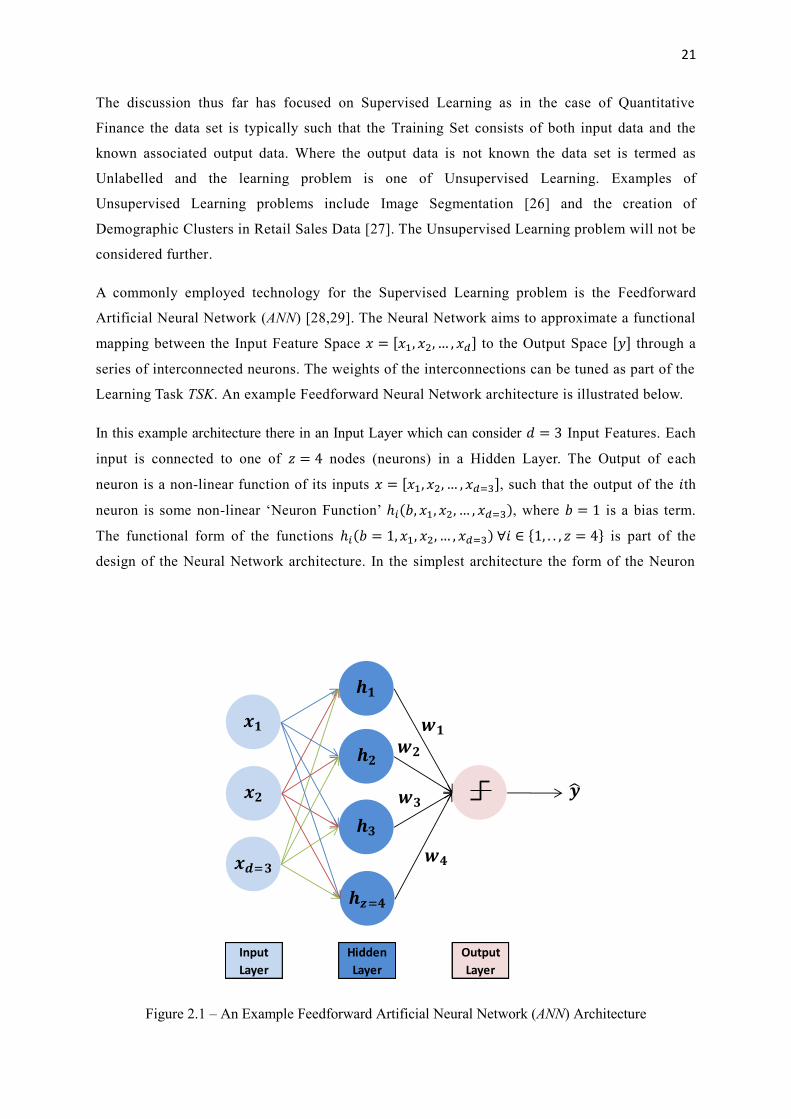
A commonly employed technology for the Supervised Learning problem is the Feedforward

Artificial Neural Network (ANN) [28,29]. The Neural Network aims to approximate a functional

mapping between the Input Feature Space 𝑥 = [𝑥1, 𝑥2, … , 𝑥𝑑] to the Output Space [𝑦] through a

series of interconnected neurons. The weights of the interconnections can be tuned as part of the

Learning Task TSK. An example Feedforward Neural Network architecture is illustrated below.

In this example architecture there in an Input Layer which can consider 𝑑 = 3 Input Features. Each

input is connected to one of 𝑧 = 4 nodes (neurons) in a Hidden Layer. The Output of each

neuron is a non-linear function of its inputs 𝑥 = [𝑥1, 𝑥2, … , 𝑥𝑑=3], such that the output of the 𝑖th

neuron is some non-linear ‘Neuron Function’ ℎ𝑖(𝑏, 𝑥1, 𝑥2, … , 𝑥𝑑=3), where 𝑏 = 1 is a bias term.

The functional form of the functions ℎ𝑖(𝑏 = 1, 𝑥1, 𝑥2, … , 𝑥𝑑=3) ∀𝑖 ∈ {1, . . , 𝑧 = 4} is part of the

design of the Neural Network architecture. In the simplest architecture the form of the Neuron

Figure 2.1 – An Example Feedforward Artificial Neural Network (ANN) Architecture

Input Hidden Output

Layer Layer Layer

=

=

22

Function may be restricted to polynomials of some degree, at the other extreme each function

may itself be a weighted composition of other more complex functions.

In the Output Layer a weighted combination of each output in the Hidden Layer is formed. A

Neural Network can be employed as either a Predictor to be used in a Regression Problem or as

a classifier to be used in a Classification Problem. In either problem the output �̂� would be of the

form �̂� = 𝐾(∑ 𝑤𝑖ℎ𝑖(𝑏 = 1, 𝑥1, 𝑥2, … , 𝑥𝑑)𝑖=𝑧𝑖=1 ) where {𝑤1, 𝑤2, … , 𝑤𝑧} are the weights applied to the

𝑧 outputs of the Hidden Layer. Here 𝐾 is an Activation Function, such as a Hyperbolic Tangent

Function, used for normalisation such that −1 ≤ �̂� ≤ 1. In the case of a Classification Problem

the output of the Activation Function is discretised to create a mapping to classes.

The Machine Learning Task (TSK) is then one to determine the optimal, according to some

Performance Measure (PER), weights 𝑤 = {𝑤1, 𝑤2, … , 𝑤𝑧} and functional forms ℎ𝑖(𝑏 =

1, 𝑥1, 𝑥2, … , 𝑥𝑑) ∀𝑖 ∈ {1, . . , 𝑧} based on the Training Set that forms the Experience (EXR). This

Machine Learning Task (TSK) is a complex optimisation problem involving a search through a

massive solution space. A common learning approach is to aim to minimise the Mean Square Error

(MSE) between the Neural Network output �̂�[𝑛] and the expected output 𝑦[𝑛] across a Training Set

of 𝑁 Training Samples, where each Training Sample is of the form specified in Equation 2.1.

The process of Mean Square Error minimisation is commonly carried out by employing a type of

Gradient Descent technique, this is known as The Backpropagation Algorithm for Training.

Other approaches to the Learning Task (TSK) optimisation problem are based on Genetic

Algorithms [30], Simulated Annealing [31] and Particle Swarm Optimisation [32].

An extension to the ANN architecture is the Radial Basis Function Neural Network (RBFNN). In the

RBFNN Architecture [33] the non-linear ‘Neuron Function’ ℎ𝑖(𝑏, 𝑥1, 𝑥2, … , 𝑥𝑑) takes the form

ℎ𝑖 = 𝑃(‖𝑥 − 𝑐𝑖‖22) (2.2)

where 𝑥 = [𝑏 = 1, 𝑥1, 𝑥2, … , 𝑥𝑑] and 𝑐𝑖 are vectors of dimension 𝑑 + 1. The vector 𝑐𝑖 is the Centre

Vector for the 𝑖th neuron and will be optimized over the Training Set as part of the Learning

Task (TSK). The function P typically takes the form of an Exponential Function and ‖∙‖22 is the

square of the Euclidean Distance between the vectors 𝑥 and 𝑐𝑖.

A further extension to the Artificial Neural Network (ANN) framework is the Recurrent Neural

Network (RNN) Architecture [34] in which the delayed outputs of the hidden layers are fed-back into

the network along with the inputs. Such RNN architectures allow the network to exhibit a memory

effect which can be useful for the processing of time series data. The example ANN architecture of

Figure 2.1 has just a single hidden layer, in the case that there are multiple hidden layers the

23

architecture is termed a Deep Neural Network (DNN) [35]. The use of a DNN allows the modelling of

a higher level of data abstraction as required for Deep Learning Problems [36]. However the DNN

architecture can be prone to overfitting as the extra hidden layers allow the fitting of rare ‘noise like’

dependencies in the data.

A competing technology to the Neural Network is the Support Vector Machine (SVM) [37].

Consider again an Input Feature space consisting of 𝑑 Input Features and a Training Set of 𝑁

Training Samples with the 𝑛th Sample 𝑇[𝑛] taking the form specified in Equation 2.1. In a

Classification Problem the outputs 𝑦[𝑛] ∀𝑛 ∈ {1, . . , 𝑁} for the 𝑁 Training Samples will be able to

take one of 𝐶 discrete classes. It would then be possible to represent the Training Set as a

collection of labelled points in a 𝑑 dimensional space with each point taking one of 𝐶 labels. The

SVM methodology is based on a one-versus-many classification approach. For a particular

desired class of label 𝑐 the SVM Learning Task (TSK) aims to create a separating Hyperplane in

the 𝑑 dimensional space between those Training Samples for which the output 𝑦[𝑛] = 𝑐 and

those Training Samples for which the output 𝑦[𝑛] ≠ 𝑐. For a Classification Problem with 𝐶

classes there will be 𝐶 − 1 separating Hyperplanes created during the Learning Task (TSK). The

Performance Measure (PER) for the creation of the 𝑐th Hyperplane will be the sum of (i)-the

minimum distance between the Hyperplane and Training Samples for which 𝑦[𝑛] = 𝑐 and (ii)-the

minimum distance between the Hyperplane and Training Samples for which 𝑦[𝑛] ≠ 𝑐. The SVM

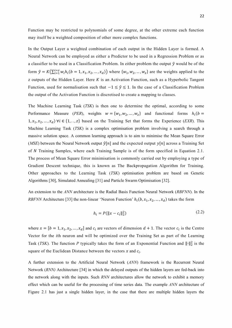
Task (TSK) will aim to maximise this measure (PER). The creation of such a Maximum Margin

Hyperplane is illustrated below for the simplified case of a 𝑑 = 2 dimension feature space.

Figure 2.2 – An Illustration of Separating Hyperplanes in a 𝑑 = 2 Dimension Feature Space

0 0.1 0.2 0.3 0.4 0.5 0.6 0.7 0.8 0.9 10

0.1

0.2

0.3

0.4

0.5

0.6

0.7

0.8

0.9

1

Feature 1

Featu

re 2

class = c

class not= c

24

Two example separating Hyperplanes are shown in Figure 2.2. The Green Hyperplane does

separate the data according to classes, however it is the Purple Maximum Margin Hyperplane

which achieves the maximal separation by the measure PER described above. In general the

dimension 𝑑 may be large. The solution of the Maximum Margin Hyperplane is a complex task

and involves the formulation of a Primal and Dual task which leads to a set of Karush–Kuhn–

Tucker (KKT) conditions [38]. The solution of the KKT problem is often carried out using a

numerical Gradient Descent type method or more efficiently by using the Sequential Minimal

Optimization (SMO) Algorithm [39]. The optimal Maximum Margin Hyperplane, forms a linear

separating boundary between the class 𝑐 and the other classes. In the more common case that a

non-linear separating boundary is required a mapping can be created from the 𝑑 dimension

feature space to a higher dimensional space by employing the so called Kernel Trick [40]. A

linear separating boundary in the higher dimensional space would then be equivalent to a non-

linear boundary in the original 𝑑 dimension feature space. Following the training of an SVM,

classification of an input data sample 𝑥[𝑚] = [𝑥1[𝑚], 𝑥2[𝑚],… , 𝑥𝑑[𝑚]] requires a simple

determination of where 𝑥[𝑚] is located in reference to the set of 𝐶 − 1 separating Hyperplanes.

Neural Networks and the Support Vector Machine (SVM) exist as competing technologies. Under

comparison for the same datasets the SVM has been shown [41,42] to achieve slightly higher

accuracies than typical Neural Networks. However, the SVM is a one-versus-many classifier and

where the number of classes 𝐶 is large the optimisation may be computationally inefficient.

2.1.2 Probabilistic Modelling: Graphical Models and Graph Theory

Probabilistic Graphical Models (PGM) provides a convenient framework to compactly represent

real world problems that are driven by uncertainty. The subject is vast and evolving and a

complete overview would be beyond the scope of this Thesis. The summary presentation will

focus on the two main classes of PGM which are Bayesian Networks and Markov Networks.

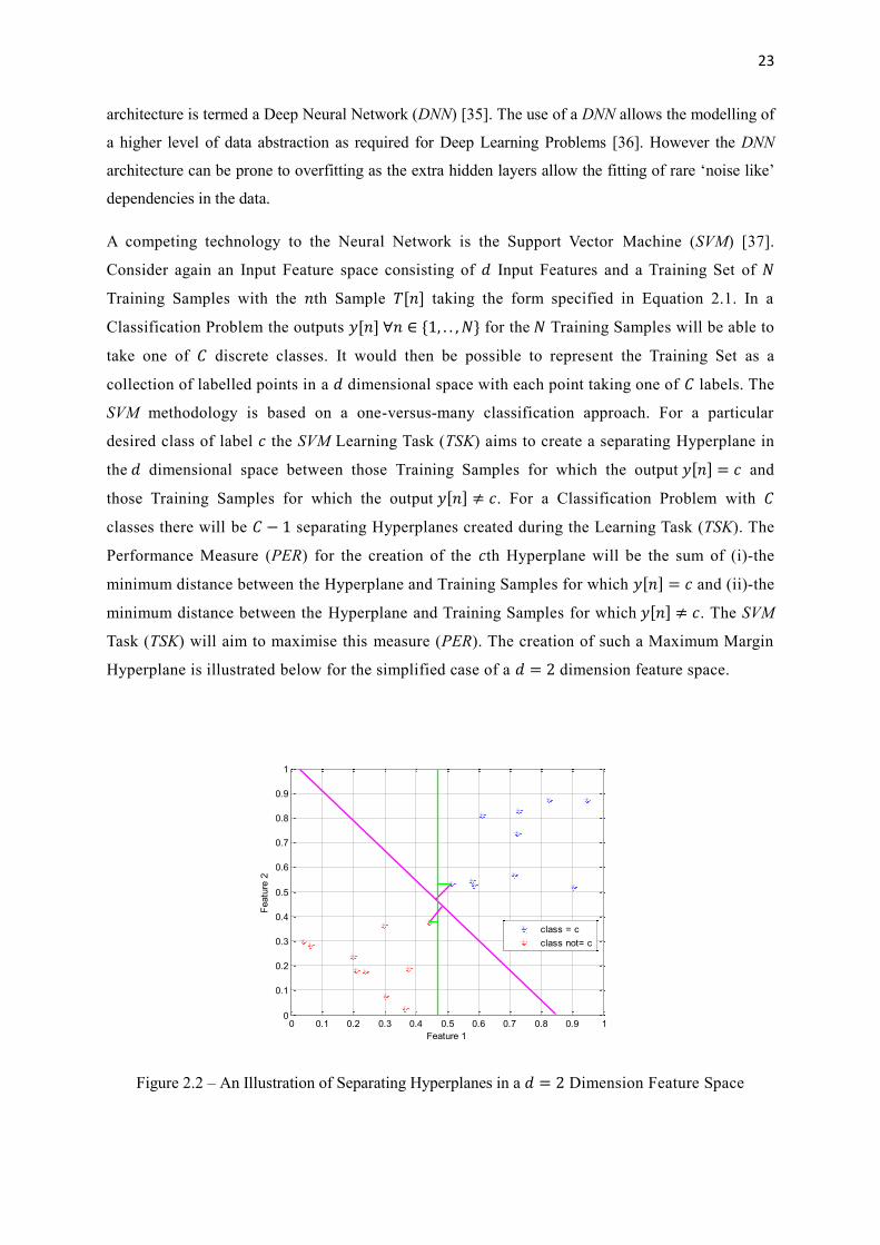
Consider a Joint Probability Distribution 𝑃 that is defined over a set of 𝑑 Random Variables

𝑋 = {𝑋1, 𝑋2, … , 𝑋𝑑}. A Bayesian Network [43] would be a Directed Acyclic Graph (DAG)

representation of the dependencies of the random variables. To motivate the presentation

consider an example with is adapted from Murphy [44]. The 𝑑 = 4 random variables are (1) The

Sky Was Cloudy, (2) It Was Raining, (3) The Sprinkler Was On and (4) The Ground Is Wet; in this

modified example the Sprinkler is assumed to operate independently of the weather. A Bayesian

Network can be used to represent the joint distribution 𝑃 as shown in Figure 2.3. The directed

connections in the DAG show the influence of random variables upon each other. In the model in

Figure 2.3 the random variable (2) It Was Raining is directly influenced by (1) The Sky Was

25

Figure 2.3 – An Example Bayesian Network with 𝑑 = 4 Random Variables

Cloudy. The random variable (4) The Ground Is Wet is only indirectly influenced by (1) The Sky

Was Cloudy. The random variable (3) The Sprinkler Was On is independent of (2) It Was

Raining. Although intuitive logic would tell us that the random variable (2) It Was Raining is

independent of the random variable (3) The Sprinkler Was On, this is not actually inferable from

the DAG. The only inferable assumption is that the random variable (2) It Was Raining is

conditionally independent of the random variable (3) The Sprinkler Was On given the random

variable (1) The Sky Was Cloudy. The DAG is a convenient representation of the joint

distribution which can be simplified to

𝑃(𝑋1, 𝑋2, 𝑋3, 𝑋4) = 𝑃(𝑋4|𝑋2, 𝑋3)𝑃(𝑋2|𝑋1)𝑃(𝑋3)𝑃(𝑋1) (2.3)

The Bayesian Network therefore provides a convenient graphical representation of the dependencies

in the Joint Distribution 𝑃(𝑋1, 𝑋2, 𝑋3, 𝑋4). The Machine Learning Task (TSK) is then a twofold

task to learn (1) The Structure of the Network and (2) The Distribution of the Conditional

Random Variables. These two parts of the Learning Task (TSK) are connected since the structure

of the network determines the interconnections of the random variables {𝑋1, 𝑋2, … , 𝑋𝑑} and then

in turn which conditional distributions 𝑃(𝑋𝐴|𝑋𝐵) need to be learned. Simultaneously the

optimisation of the network structure requires a-priori knowledge of the distributions.

In the simplest case the network structure is specified by a human expert. In order to fully

automatically learn the network structure a search strategy can be employed as part of the Task

(TSK). An exhaustive search can be carried out by a method such as Markov Chain Monte Carlo

[45], the Performance Measure (PER) to be maximized is the posterior probability of the

structure given the Training Set 𝑇; such brute force optimisation is exponential in the number of

26

Random Variables 𝑑. An alternative more efficient approach [46] attempts to find a structure

which maximises as a Performance Measure (PER) the Mutual Information between variables.

Having determined a Network Structure it is then necessary to learn all of the conditional

distributions that form the structure. In the example of Figure 2.3 the remaining part of the

Learning Task (TSK) is to estimate the four distributions 𝑃(𝑋4|𝑋2, 𝑋3), 𝑃(𝑋2|𝑋1), 𝑃(𝑋3) and

𝑃(𝑋1). It is common to limit the choice of distributions to be either discrete or to be a member of

the Elliptical Family of Probability Distributions, this is in order to simplify the Learning Task (TSK).

The Training Set 𝑇 can then be used as part of an Experience (EXR) to learn the parameters of the

distributions, the Performance Measure (PER) to be maximized is the Likelihood.

Having established the Graphical Model it is then possible to determine the probability of causal

variables given evidence. For example to determine the probability that (3) The Sprinkler Was

On given (4) The Ground is Wet. It is also possible to carry out inferences such as the estimation

of the Most Probable Explanation (MPE) [43], 𝑎𝑟𝑔𝑚𝑎𝑥𝑋1,𝑋2,𝑋3,𝑋4 𝑃(𝑋1, 𝑋2, 𝑋3, 𝑋4).

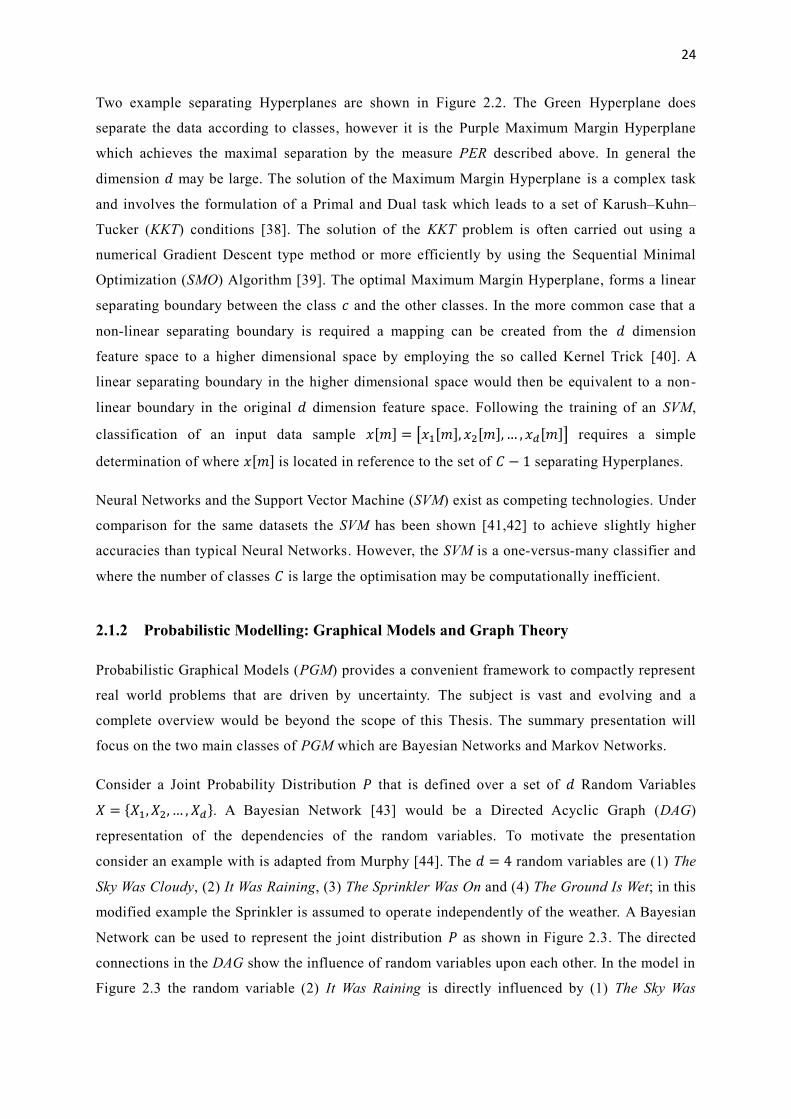
A Markov Network or Markov Chain [47] is a Graphical Model representation of a system

which can exist in only a finite number of states. The system must obey the Markov Property

such that what happens at the next timestamp depends only on the current state of the system

and is independent of how the current state had arisen. At each discrete timestamp 𝑡 the system

can probabilistically transition from its current state 𝑆[𝑡] to the state at the next timestamp

𝑆[𝑡 + 1]. Consider as an example a system to model the position of a person in an apartment, the

system can exist in only one of 𝑑 = 4 states such that the State Set is 𝑆[𝑡] ∈ {𝑠1, 𝑠2, … , 𝑠𝑑=4} ∀𝑡.

In this example the states are (𝑠1) Person is in the Hall, (𝑠2) Person is in the Living Room, (𝑠3)

Person is in the Bedroom and (𝑠4) Person is in the Bathroom. If it is assumed that each room is

only connected to the Hall and that the person moves from room to connected room or stays in

their current room with an equal probability then the model can be represented as in Figure 2.4.

Figure 2.4 – An Example Markov Network with 𝑑 = 4 States

27

The Learning Task (TSK) is again a twofold task to learn (1) The Possible States of the Network

and (2) The Transition Probabilities Between States. The structure of the network in terms of the

set of possible states is typically much easier to learn for a Markov Network than for a Bayesian

Network as the set of states and their interconnections can often be directly observed. The bulk

of the Learning Task (TSK) is then the determination of the 𝑑 × 𝑑 dimensioned Transition Matrix

ℙ of Transition Probabilities. The Probability 𝑃{𝐴,𝐵} corresponds to the conditional probability of

the event that 𝑆[𝑡] = 𝑠𝐵 given that 𝑆[𝑡 − 1] = 𝑠𝐴 which can otherwise be written as

𝑃{𝐴,𝐵} = 𝑃(𝑆[𝑡] = 𝑠𝐵|𝑆[𝑡 − 1] = 𝑠𝐴). It is commonly assumed that such probabilities are

discreetly distributed or have a distribution that falls in the Elliptical Family. The Training Set 𝑇

can be used as part of an Experience (EXR) to learn the parameters of the distributions, the

Performance Measure (PER) to be maximized is the Likelihood. Having determined the structure

of the network and the Transition Matrix ℙ it is then possible to determine the distribution of the

long term equilibrium state of the system 𝑃(𝑆[∞]) as the Principle Eigenvector of ℙ.

2.1.3 Online Learning

The Supervised Learning problem considered in the case of a Neural Network or a Support

Vector Machine is a Batch Learning problem. The learning Experience (EXR) involves the

presentation of the complete Training Set 𝑇 of 𝑁 Training Samples as a Batch of Data such that

the Learning Task (TSK) is an optimisation of a functional mapping between the Input Feature

Space 𝑥 = [𝑥1, 𝑥2, … , 𝑥𝑑] to the Output Space [𝑦] across the Training Set 𝑇 of size 𝑁 Samples in a

one shot fashion. In the case that a new Training Sample 𝑇[𝑁 + 1] becomes available the

Learning Task (TSK) must be recompleted from the beginning over the expanded batch of size

𝑁 + 1. This creates two potential problems; the first is the time of retraining and the second is

the requirement to store the full Training Set.

Consider an application where data arrives synchronously and a Machine Learning technology

has been trained using the first 𝑁 pieces of data, as the Input Features of data sample 𝑁 + 1,

𝑥[𝑁 + 1] = [𝑥1[𝑁 + 1], 𝑥2[𝑁 + 1], … , 𝑥𝑑[𝑁 + 1]] become available the Machine could be used to

predict the associated output �̂�[𝑁 + 1]. When the true output 𝑦[𝑁 + 1] becomes available an

extra Training Sample 𝑇[𝑁 + 1] ∶= {[𝑥1[𝑁 + 1], 𝑥2[𝑁 + 1], … , 𝑥𝑑[𝑁 + 1]], [𝑦[𝑁 + 1]]} can be

used to improve upon the original functional mapping between the Input Feature Space 𝑥 =

[𝑥1, 𝑥2, … , 𝑥𝑑] to the Output Space [𝑦]. However, it may often be the case that there is

insufficient time to complete a full retraining before the Input Features of data sample 𝑁 + 2

become available and the next prediction or classification must take place. Also it many

applications it may not be possible to store the full dataset due to data storage limitations.

28

In an Online Learning [48] setting the optimised Predictor at timestamp 𝑁 is updated at

timestamp 𝑁 + 1 using only knowledge of the state of the Predictor at timestamp 𝑁 and the

newly available Training Sample 𝑇[𝑁 + 1] ∶= {[𝑥1[𝑁 + 1], 𝑥2[𝑁 + 1], … , 𝑥𝑑[𝑁 + 1]], [𝑦[𝑁 + 1]]}.

The original Training Set up to sample 𝑁 is no longer used although its characteristics are

captured in the state of the Predictor that had been optimised at timestamp 𝑁.

Approaches to Online Learning are generally categorised as either Statistical Learning Models

or Adversarial Models. In the case of Statistical Learning Models it is assumed that the arriving

data samples are Independently Identically Distributed (IID) and as such that The Environment

itself is not aware of the existence of The Learner and is not attempting to adapt to the presence

of The Learner. In the setting of Adversarial Models the Learning Task is considered as a game

between two opponents, The Learner and The Environment, both opponents are able to adapt to

the presence of the other and as such the arriving data samples will no longer be IID.

In the case that a simple weighted mapping 𝑤 = [𝑤1, 𝑤2, … , 𝑤𝑑] exists, or is at least assumed to

exist, between the Input Feature Space 𝑥 = [𝑥1, 𝑥2, … , 𝑥𝑑] and the Output Space [𝑦], the

coefficients of the mapping can be estimated in a Batch Learning setting by employing the

Linear Least Squares method [49], where the Performance Measure (PER) to be minimized is

the Mean Square Error (MSE) between the Actual Outputs {𝑦} and Estimated Outputs {�̂�} across

the Training Set of size 𝑁. The estimated weights of the mapping can be determined as

𝑤 = (𝕏𝑇𝕏)−1𝕏𝑇𝑌 (2.4)

where 𝕏 is an 𝑁 × 𝑑 matrix whose 𝑛th row is 𝑥[𝑛] = [𝑥1[𝑛], 𝑥2[𝑛], … , 𝑥𝑑[𝑛]] and 𝑌 is an 𝑁 × 1

vector whose 𝑛th entry is 𝑦[𝑛]. Here 𝕏𝑇 is the Transpose of 𝕏 and 𝕏−1 is the Matrix Inverse of

𝕏. This Batch Learning technique requires knowledge of the Full Training Set in the form of 𝕏

and 𝑌. The Statistical Learning based Online Learning counterpart of the Linear Least Squares

method is the Recursive Least Squares method which can also be shown [50] to the Minimize

the Mean Square Error (MSE) as a performance measure (PER). Having initialized such that

𝑤[0] = [1

𝑑,1

𝑑, … ,

1

𝑑], the updated estimated weight vector 𝑤 [𝑁 + 1] at the timestamp 𝑁 + 1 is

𝑤 [𝑁 + 1] = 𝑤 [𝑁] − 𝔾[𝑁 + 1]𝑥[𝑁](𝑥𝑇[𝑁]𝑤 [𝑁] − 𝑦[𝑁}) (2.5)

where 𝔾[𝑁 + 1] is a 𝑑 × 𝑑 matrix updated such that

𝔾[𝑁 + 1] = 𝔾[𝑁] −𝔾[𝑁] 𝑥[𝑁 + 1]𝑥𝑇[𝑁 + 1]𝔾[𝑁]

1 + 𝑥𝑇[𝑁 + 1]𝔾[𝑁]𝑥[𝑁 + 1] (2.6)

29

Here 𝔾[0] is initialised as the 𝑑 dimensioned Identity Matrix. The Recursive Least Squares

method is a commonly used Online Learning Technique. In the case that a richer mapping than a

simple weighted combination of the Input Feature Space 𝑥 = [𝑥1, 𝑥2, … , 𝑥𝑑] to the Output Space

[𝑦] is required, the Input Feature Space can be pre-mapped to a Higher Dimensional Functional

Space 𝑓(𝑥) and the Linear Least Squares method or Recursive Least Squares method can be

applied to determine weights which map from the new Higher Dimensional Functional Space

𝑓(𝑥) to the Output Space [𝑦]. This mapping to a Higher Dimensional Functional Space 𝑓(𝑥) may

employ the Kernel Trick [40] as is often used in the Support Vector Machine (SVM) setting. The

design of both the Linear Least Squares method and the Recursive Least Squares method is

based on Mean Square Error (MSE) Minimization and implicit to this is the assumption that the

input data are Independently Identically Distributed (IID).

In order to relax the IID assumption it is possible to turn to an Adversarial Model. The

framework of the Adversarial Model is based on a number of Hypotheses which are otherwise

called Experts. In order to motivate the presentation consider an example that is adapted from

Blum [51]. The Learning Task (TSK) is to predict if it will rain today or not at some specific

location, the Adversarial Learner has available the predictions of 𝑑 Experts, such that 𝑥[𝑁] =

[𝑥1[𝑁], 𝑥2[𝑁], … , 𝑥𝑑[𝑁]] is a vector of the predictions at timestamp 𝑁 and 𝑥𝑖[𝑁] ∈ {−1,1}∀𝑖, 𝑁.

Here 𝑥𝑖[𝑁] = 1 if the 𝑖th Expert does predict rain at timestamp 𝑁 and 𝑥𝑖[𝑁] = −1 otherwise. The

overall prediction of rain today �̂�[𝑁] is based on a weighted combination of the predictions of

the 𝑑 Experts, such that

�̂�[𝑁] = sgn(𝑤𝑇[𝑁]𝑥[𝑁]

|𝑤[𝑁]|) (2.7)

where 𝑤[𝑁] = [𝑤1[𝑁], 𝑤2[𝑁], … ,𝑤𝑑[𝑁]] with 𝑤𝑖[𝑁] the weight applied to the prediction of the

𝑖th Expert at timestamp 𝑁. Here sgn(. ) is the Sign Operator and takes the value of +1 if its

operand is greater than or equal to zero and takes the value of −1 otherwise; in addition |𝑤[𝑁]|

is the ℓ1-norm of 𝑤[𝑁] included for regularisation. At the end of timestamp 𝑁 the true value of

𝑦[𝑁] will be known as it will be known if it did (𝑦[𝑁] = +1) or did not (𝑦[𝑁] = −1) rain.

Following the revelation of the true value of 𝑦[𝑁] each of the Experts is able to then update their

predictive models such that each 𝑥𝑖[𝑁 + 1] would be able to incorporate knowledge of 𝑦[𝑁] and

also of the prediction of the Learner �̂�[𝑁]. It would typically be the case that each Expert would

follow some form of Statistical Learning Model. It is in the update of the weight vector 𝑤[𝑁 +

1] that an Adversarial Model is considered. Adversarial Models often consider a Regret Function

based on the differences between the Predicted Values from the Experts

𝑥[𝑁] = [𝑥1[𝑁], 𝑥2[𝑁], … , 𝑥𝑑[𝑁]] and the True Value 𝑦[𝑁].

30

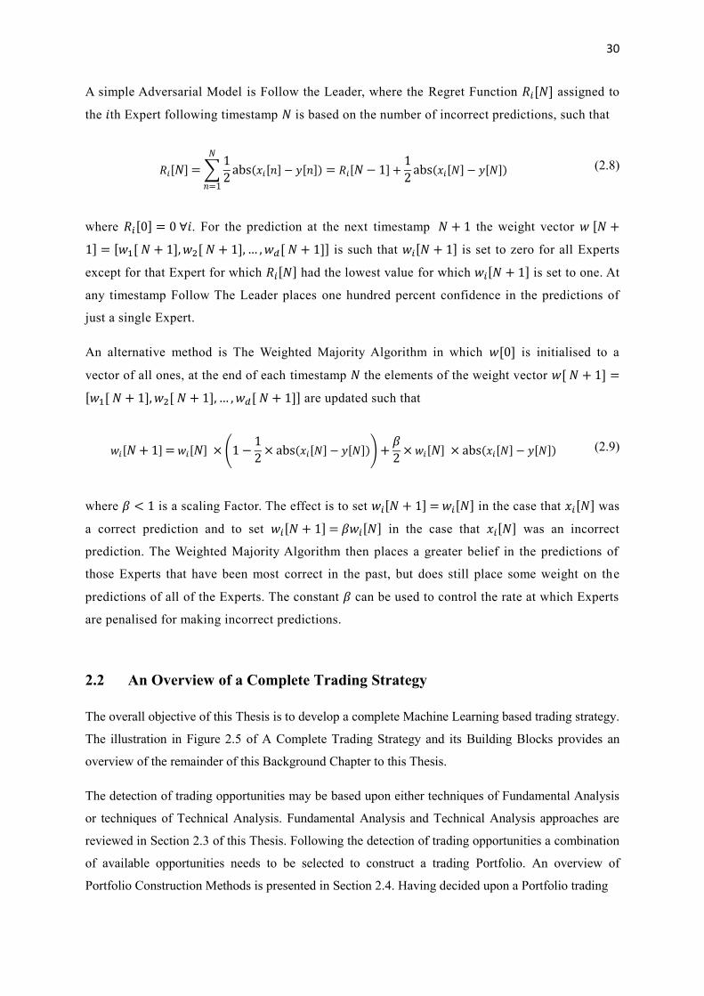
A simple Adversarial Model is Follow the Leader, where the Regret Function 𝑅𝑖[𝑁] assigned to

the 𝑖th Expert following timestamp 𝑁 is based on the number of incorrect predictions, such that

𝑅𝑖[𝑁]= ∑1

2abs(𝑥𝑖[𝑛] − 𝑦[𝑛])

𝑁

𝑛=1

= 𝑅𝑖[𝑁− 1] +1

2abs(𝑥𝑖[𝑁] − 𝑦[𝑁]) (2.8)

where 𝑅𝑖[0] = 0 ∀𝑖. For the prediction at the next timestamp 𝑁 + 1 the weight vector 𝑤 [𝑁 +

1] = [𝑤1[ 𝑁 + 1], 𝑤2[ 𝑁 + 1], … ,𝑤𝑑[ 𝑁 + 1]] is such that 𝑤𝑖[𝑁 + 1] is set to zero for all Experts

except for that Expert for which 𝑅𝑖[𝑁] had the lowest value for which 𝑤𝑖[𝑁 + 1] is set to one. At

any timestamp Follow The Leader places one hundred percent confidence in the predictions of

just a single Expert.

An alternative method is The Weighted Majority Algorithm in which 𝑤[0] is initialised to a

vector of all ones, at the end of each timestamp 𝑁 the elements of the weight vector 𝑤[ 𝑁 + 1] =

[𝑤1[ 𝑁 + 1], 𝑤2[ 𝑁 + 1], … ,𝑤𝑑[ 𝑁 + 1]] are updated such that

𝑤𝑖[𝑁+ 1]=𝑤𝑖[𝑁] × (1 −1

2× abs(𝑥𝑖[𝑁] − 𝑦[𝑁]))+

𝛽

2×𝑤𝑖[𝑁] × abs(𝑥𝑖[𝑁] − 𝑦[𝑁]) (2.9)

where 𝛽 < 1 is a scaling Factor. The effect is to set 𝑤𝑖[𝑁 + 1] = 𝑤𝑖[𝑁] in the case that 𝑥𝑖[𝑁] was

a correct prediction and to set 𝑤𝑖[𝑁 + 1] = 𝛽𝑤𝑖[𝑁] in the case that 𝑥𝑖[𝑁] was an incorrect

prediction. The Weighted Majority Algorithm then places a greater belief in the predictions of

those Experts that have been most correct in the past, but does still place some weight on the

predictions of all of the Experts. The constant 𝛽 can be used to control the rate at which Experts

are penalised for making incorrect predictions.

2.2 An Overview of a Complete Trading Strategy

The overall objective of this Thesis is to develop a complete Machine Learning based trading strategy.

The illustration in Figure 2.5 of A Complete Trading Strategy and its Building Blocks provides an

overview of the remainder of this Background Chapter to this Thesis.

The detection of trading opportunities may be based upon either techniques of Fundamental Analysis

or techniques of Technical Analysis. Fundamental Analysis and Technical Analysis approaches are

reviewed in Section 2.3 of this Thesis. Following the detection of trading opportunities a combination

of available opportunities needs to be selected to construct a trading Portfolio. An overview of

Portfolio Construction Methods is presented in Section 2.4. Having decided upon a Portfolio trading

31

Figure 2.5 - A Complete Trading Strategy and its Building Blocks

orders are then generated and these need to be executed, an overview of Market Order Book Structure

and Trade Execution Methods is presented in Section 2.5. The overall objective of this Thesis is to

develop a complete Machine Learning based trading strategy. Achieving this objective would require

the interaction of the three building blocks identified in Figure 2.5.

2.3 Trading Opportunity Detection

In this section a review of the current state of the art of methods for the detection of trading

opportunities is presented. The section begins with an overview of Fundamental and Technical

Analysis techniques and a discussion of how they may be applied in a setting without Machine

Learning. This is followed by a review of the current state of the art of the application of Machine

Learning into these domains.

2.3.1 Overview of Trading Opportunity Detection

The Fundamental Analysis approach attempts to value a stock through the analysis of Microeconomic

and Macroeconomic factors that are pertinent to that stock. Microeconomic factors may include

information that has been extracted from the annual report of the company as well as information that

has been extracted from the reports of competitor firms or from the reports of industry analysts.

Macroeconomic factors may include measures of country specific data or global economic health as

well as government policies. The Input Features of Fundamental Analysis may be quantitative factors

such as Accounting Ratios or Gross Domestic Product (GDP) figures. The Input Features may also be

qualitative such as a human analyst’s interpretation of the ability of senior management to transform a

company. The role of the Fundamental Analyst is to process such fundamental data and to forecast a

Market Data Database

Original Contributions in

Thesis Chapter 3

Block 2 : Portfolio

Construction

Background in Thesis Section

2.4


Thesis Chapter 4

Block 3 : Order Entry Timing


2.5


Thesis Chapter 5

Block 1 : Trading Opportunity

Detection


2.3

Flow ofTrading

Opportunities

Flow ofMarket Data

Flow ofMarket Data

Flow ofMarket Data

Flow ofTrade

Orders

32

target price for a particular stock over a time horizon, the target price would then be compared against

the current market price and a decision to Buy or Sell the stock would then be made.

Fundamental Analysis is based on a belief that an analyst is seeing the details ‘correctly’ and that

others will see the same details equally ‘correctly’ at some point in the future, this is necessary in

order for the market to bring the stock price into line with the analysts forecast. Even if a Fundamental

Analyst is correct, the time horizon required for the stock price to move to where it should be can be

long. The input data required for Fundamental Analysis is often difficult to obtain. Digitised

accounting information from the financial reports of companies can now be obtained from a data

provider such as CapitalIQ [52]. However, obtaining other more subjective data requires a great deal

of effort and information resource and as such this type of subjective analysis is typically only carried

out by large institutions who have either achieved economies of scale by managing large Portfolios or

by firms who are able to sell their analysis in order to be able to recover their research costs.

Accounting data may also be affected by quality issues such as accounting anomalies [53,54] and data

revisions [55]. For all of these reasons many analysts instead prefer to focus on Technical Analysis.

The field of Technical Analysis focusses on the prediction of the movements of security prices by

searching for patterns in historical price charts and traded volume data. Technical Analysis is formally

considered to be analysis that is based solely upon information that can be directly observed from the

market. The types of direct Market Data used for Technical Analysis will typically be more accurate

and less subject to data collection issues and revision than the data used for Fundamental Analysis.

The core concept of Technical Analysis is that prices are determined by investor supply and demand

for assets. Such supply and demand is driven in part by rational behaviour, for example by traders

reacting to new information that may itself be processed in a Fundamental Analysis context. Supply

and demand may also be driven by irrational behaviour, for example by traders following the herd and

copying a popular trade with no other supporting reason to trade.

It is the existence of such rational and irrational behaviour that forms the underlying reason for

conducting Technical Analysis. The premise is that rational behaviour will be conducted by a number

of participants and this would take a period of time sufficiently long to allow a trend to be spotted. At

the same time detectable irrational behaviour will exist and this would also provide trading

opportunities. In short Technical Analysis is based on the rationality of rational players and on the

rationalisation of the irrationality of others. The underlying assumption of Technical Analysis is that

whilst the causes of changes in supply and demand, or in rational and irrational behaviour, are

difficult to determine, the actual shifts can be directly observed in market information.

The causes of irrational trading behaviour and the effects in terms of deviations from the EMH have

been well studied [56,57] in the context of behavioural finance. A typical example of irrational trading

behaviour is the so called hot hand fallacy [58] whereby investors prefer to buy more of their well

33

performing (hot) stocks and to sell their (cold) losers, such behaviour would lead to the creation of a

Momentum Anomaly as the price of a well performing stock is further increased by additional buying.

Another common example of irrational trading behaviour is herding whereby traders simply follow

the herd and copy a popular trade with no other supporting reason to trade. Herding behaviour would

initially lead to the creation of a Momentum Anomaly, this would typically be followed in turn by an

Overreaction Anomaly as buyers turn into sellers en-masse. The famous gamblers fallacy [59] is

another common trading behaviour, here a trader irrationally holds out for a directional reversal in the

face of a losing trade. Losing traders can only absorb losses up to a limit and all losing traders will

eventually look to exit their positions. Losing traders often look to exit their trades around the same

time thus spurring a Momentum Anomaly. From a Technical Analysis standpoint the exact causes of

irrational trading behaviour are not of great importance, it is only necessary to understand and then

detect the effects in terms of the creation of Momentum or Overreaction Trading Anomalies.

Approaches to Technical Analysis

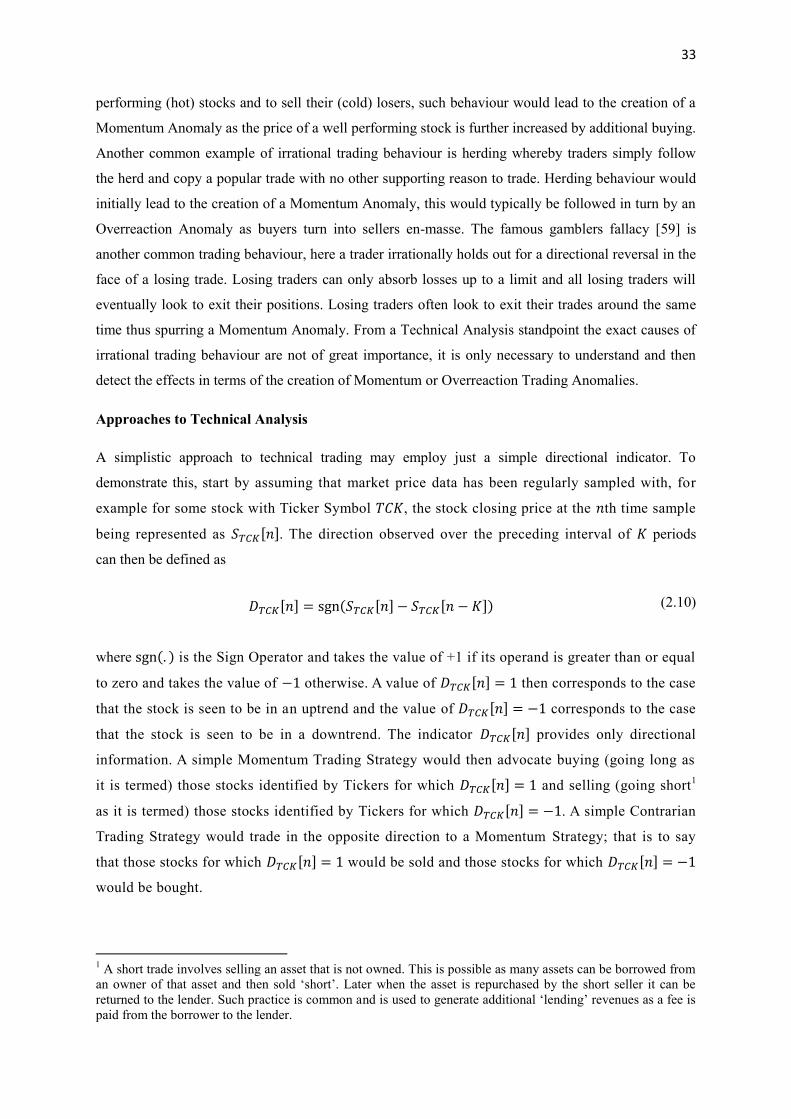
A simplistic approach to technical trading may employ just a simple directional indicator. To

demonstrate this, start by assuming that market price data has been regularly sampled with, for

example for some stock with Ticker Symbol 𝑇𝐶𝐾, the stock closing price at the 𝑛th time sample

being represented as 𝑆𝑇𝐶𝐾[𝑛]. The direction observed over the preceding interval of 𝐾 periods

can then be defined as

𝐷𝑇𝐶𝐾[𝑛] = sgn(𝑆𝑇𝐶𝐾[𝑛] − 𝑆𝑇𝐶𝐾[𝑛 − 𝐾]) (2.10)

where sgn(. ) is the Sign Operator and takes the value of +1 if its operand is greater than or equal

to zero and takes the value of −1 otherwise. A value of 𝐷𝑇𝐶𝐾[𝑛] = 1 then corresponds to the case

that the stock is seen to be in an uptrend and the value of 𝐷𝑇𝐶𝐾[𝑛] = −1 corresponds to the case

that the stock is seen to be in a downtrend. The indicator 𝐷𝑇𝐶𝐾[𝑛] provides only directional

information. A simple Momentum Trading Strategy would then advocate buying (going long as

it is termed) those stocks identified by Tickers for which 𝐷𝑇𝐶𝐾[𝑛] = 1 and selling (going short1

as it is termed) those stocks identified by Tickers for which 𝐷𝑇𝐶𝐾[𝑛] = −1. A simple Contrarian

Trading Strategy would trade in the opposite direction to a Momentum Strategy; that is to say

that those stocks for which 𝐷𝑇𝐶𝐾[𝑛] = 1 would be sold and those stocks for which 𝐷𝑇𝐶𝐾[𝑛] = −1

would be bought.

1 A short trade involves selling an asset that is not owned. This is possible as many assets can be borrowed from

an owner of that asset and then sold ‘short’. Later when the asset is repurchased by the short seller it can be

returned to the lender. Such practice is common and is used to generate additional ‘lending’ revenues as a fee is

paid from the borrower to the lender.

34

A study [60] of the profitability of Momentum and Contrarian Trading Strategies for stocks

listed in the USA shows that over the majority of the time period for the years 1926 to 1989

profits could have been achieved through following a Momentum Strategy, although at other

times a Contrarian Strategy would have been profitable. However, it is the determination of

when to apply a Momentum Strategy and when to apply a Contrarian Strategy that poses the real

challenge. In addition it may be the case that the price movements of a particular stock are

behaving efficiently and as such neither a Momentum nor a Contrarian Strategy would be

expected to yield non-zero profits. Although placing trades in an efficient market would be

expected to yield on average zero trading profit, trading under such conditions would still incur

trading costs and should therefore be avoided. A single directional indicator provides only basic

information and consequently other technical indicators have been developed. An exhaustive list of

indicators would be beyond the scope of this Thesis, however a summary of some of the more

common and interesting indicators is given below. The list includes many Technical Analysis

indicators that have been later applied in a Machine Learning setting in the literature.

Moving Averages – A simple 𝐾 point retrospective moving average of a stock price can be defined as

𝑆�̅�𝐶𝐾,𝐾[𝑛] =1

𝐾∑ 𝑆𝑇𝐶𝐾[𝑛 − 𝑘]

𝐾−1

𝑘=0

(2.11)

A simple trading strategy [61] would advocate buying a stock that is trading above its 𝐾 = 200 day

Moving Average and selling a stock otherwise. Such a strategy had shown success prior to the

mid-1990s but returns were seen to diminish over time and this may have been due to more and

more traders following the same strategy. Other strategies may consider a combination of

Moving Averages of different lengths and another common strategy [62] looks at the evolution

of a number of Moving Averages and advocates placing a buy trade when all considered

averages are moving upwards simultaneously.

Price Oscillator – The Price Oscillator is defined by a ratio of Moving Averages, such as

𝑂𝑇𝐶𝐾,𝐾,𝐿[𝑛] =𝑆�̅�𝐶𝐾,𝐾[𝑛]

𝑆�̅�𝐶𝐾,𝐿[𝑛]− 1 (2.12)

where 𝐾 < 𝐿. The case that the shorter duration Moving Average is greater than the longer duration

moving average would correspond to a scenario of upside Momentum and a Price Oscillator greater

than zero. The case that the shorter duration moving average is lower than the longer duration moving

average would correspond to a scenario of downside Momentum and a Price Oscillator less than zero.

A typical Price Oscillator based strategy would advocate buying a stock when the Oscillator is greater

35

than some threshold and selling when the Oscillator is below some other threshold. At the core of the

Price Oscillator method is the detection of Momentum Anomalies.

Disparity Indicator – In a similar fashion to the Price Oscillator a Disparity Indicator measure would

be defined as a ratio of the current stock price to a Moving Average, such as

𝑄𝑇𝐶𝐾,𝐹[𝑛] =𝑆𝑇𝐶𝐾[𝑛]

𝑆�̅�𝐶𝐾,𝐾[𝑛]− 1 (2.13)

As with the Price Oscillator a Positive Disparity would correspond to upside Momentum and a level

above some threshold could be used to signal a buy trade. A Negative Disparity would correspond to

downside Momentum and a level below some threshold could be used to signal a sell trade. The focus

of trading strategies based upon the Disparity Indicator is also the detection of Momentum Anomalies.

Fast Stochastic Indicator – The Stochastic Indicator [63] can be used as a measure of the position of

the current stock price within the range of observed prices over the preceding 𝐾 trading days, such as

𝑌𝑇𝐶𝐾,𝐾[𝑛] =𝑆𝑇𝐶𝐾[𝑛] − 𝑆 ↓𝑇𝐶𝐾,𝐾 [𝑛]

𝑆 ↑𝑇𝐶𝐾,𝐾 [𝑛] − 𝑆 ↓𝑇𝐶𝐾,𝐾 [𝑛] (2.14)

where 𝑆 ↓𝑇𝐶𝐾,𝐾 [𝑛] is the lowest price observed over a period of the 𝐾 trading days preceding 𝑛

and 𝑆 ↑𝑇𝐶𝐾,𝐾 [𝑛] is the highest price observed over that period. A typical use of the Stochastic

Indicator would employ the value 𝐾 = 14 and would signal a stock as Overbought in the case

that 𝑌𝑇𝐶𝐾,𝐾[𝑛] > 0.80 and Oversold in the case that 𝑌𝑇𝐶𝐾,𝐾[𝑛] < 0.20, these values corresponding

to the current stock price being in the upper and lower quintiles, respectively, of the recent

range. Through an identification of overbought and oversold stocks, the Fast Stochastic Indicat or

is in effect detecting the presence of Overreaction Anomalies.

The Technical Analysis indicators presented above do not form an exhaustive list. The

presentation has been confined to some common indicators and the indicators that have typically

found later application within the Machine Learning literature. The purpose of each indicator is

to give a measure of Momentum or Overreaction that could be used for the detection of

Momentum Anomalies and Overreaction Anomalies. Each measure exploits the premise that

markets are not always efficient, so the EMH does not always hold, and therefore Momentum

Anomalies or Overreaction Anomalies may exist. For each indicator a subjective threshold

would be defined upon which a decision to trade would be based. The choice of which indicators

to use under certain trading conditions would be also a subjective choice of the individual trader.

A trader may use a combination of Technical Indicators in order to make a trading decision,

36

however in combining Technical Indicators an expert trader would be guided by economic

rationality and a pure black box approach would typically be avoided.

The core premise of Technical Analysis is that either prices move in trends or exhibit anomaly

patterns that can be identified. Such trends and patterns are expected to repeat themselves over time

and as such if the start of a trend or pattern can be identified then a profitable trading opportunity can

be found. Fixed Technical Analysis systems assume that the same patterns will arise over and again

and this is a clear departure from reality. The evolving economic climate affects the success of

Technical Analysis. To maintain success a Technical Analysis based trading system needs to be

adaptive to changing market conditions, hence there is room for the application of Machine Learning

techniques. However, stock price movements are inherently non-linear and noisy and finding a

trading edge, even with a toolbox of Machine Learning techniques is a great challenge.

2.3.2 Machine Learning for Trading Opportunity Detection

The early pioneering Machine based approaches to stock selection were based on Fundamental

Analysis. The approaches attempted to apply Multiple Discriminant Analysis (MDA) methodologies

[64] to fundamental Microeconomic and Macroeconomic data. The MDA approach classifies a stock

into one of multiple groups (often Buy or Sell) and typically a Linear Discriminant Function (LDF)

[65] is used to carry out the classification. The LDF approach is known to suffer from weaknesses as

it places a strong assumption that Input Features follow a multivariate Normal Distribution and in

addition LDF techniques are unable to create non-monotonic separating boundaries. Research [66]

had shown that Neural Network methods were able to outperform MDA techniques in the prediction

of bond ratings and this in turn spurred interest in the use of such methods for stock classification.

An example [67] of a Neural Network approach to stock classification attempted to classify those

stocks for which the share price would later rise based upon just 4 quantitative Microeconomic factors

for each stock. The research showed that the Neural Network technique is able to outperform an MDA

technique on both the Training Data and on isolated Testing Data. Other similar pieces of research

[68,69] compared the use of Neural Networks and MDA techniques for the similar classification of

those stocks for which the share price will later rise, but based upon subjectively quantised pieces of

qualitative Microeconomic data such as the perceived quality of strategic plans and the new products

offerings of a firm. Again it is seen that Neural Network methods are able to outperform MDA

techniques. It is unsurprising that Neural Network methods would outperform MDA techniques when

presented with the same data. Neural Networks place no assumptions of form of structure in their

Input Features and also allow for more general functional forms for the mapping of Input Features to

37

output classifications. In short a Neural Network is a much less constrained form of classifier

technology than an MDA approach and as such would be expected to perform better.

As discussed in the previous section, the data required for Fundamental Analysis is often difficult to

obtain and can be subject to data quality issues. For these reasons it is the application of Technical

Analysis in a Machine Learning setting that has received the greater consideration. A number of

different Technical Analysis based approaches have been presented and an exhaustive review of the

complete literature would not be possible. Instead, a cross-section of the more interesting work is

presented with details provided of representative examples for each type of approach.

An early Machine Learning based approach to Technical Trading [70] attempted to apply a Back-

Propagation Type Neural Network to predict the timing at which a long (buying and then holding)

stock position should be opened and when the position should subsequently be closed (stocks sold to

zero the position). The system considered as an underlying the Tokyo Stock Exchange Prices Index

(Bloomberg Code: TOPIX INDEX). The system used as input data a five day moving average of the

Index Level (as in Equation 2.11) as well as using a five day moving average of the total traded

volume. The system also took as inputs the 5 day moving average of the Dow Jones Industrial

Average Index (Bloomberg Code: INDU INDEX) as well as the United States Dollar/Japanese Yen

Currency Exchange Rate (Bloomberg Code: JPY CURNCY) and also unspecified interest rate data.

The system output was a forecast of the index percentage price change over a subsequent one week

period. A positive forecast was used to generate a Buy Signal and a negative forecast was used to

generate a Sell Signal, although in this case the Sell Signal was only used to close any existing long

positions. The system did not allow any short trading. Over a test period of 33 months, for the period

between January 1987 to September 1989, the system if followed, would have produced a total return

of 98%, this is compared to a return of 67% for a Buy and Hold Strategy of the TOPIX INDEX.

Whilst the produced return is impressive it has only been achieved for a single test underlying and

even then only for one short test period of time. A closer inspection of the results reveals that much of

the proposed method over-performance, relative to the Buy and Hold Strategy for the benchmark

index, can be attributed to the trading decisions made during just the 3 month period leading up to

January 1988. It is possible to conclude that the results are just down to chance.

The previous approach is limited to only holding long positions in the market. Another early Back-

Propagation Type Neural Network approach [71] looked to allow both long and short positions. The

approach considered as an underlying Futures on the Standard and Poors 500 Index (Bloomberg

Code: SPX INDEX). The main inputs to the Neural Network are vectors of historical moving average

levels of SPX INDEX with several vectors of moving averages of different duration being used. In

addition to moving averages the levels of a number of other unmentioned technical indicators were

also used as input data. For the purpose of training, the subjective judgement of a human expert was

38

used to generate buy, null and sell signals based on a sample by sample visual analysis of thousands

of sets of Training Data. Each Training Sample consisted of the moving averages and other

unmentioned Technical Indicators observed at some point of time. The authors claim that such an

‘expert’ trained system has advantages over using purely historical trade performance results as the

system then has a more ‘real world’ basis. The system was painstakingly trained using around 9 years

of historical data and then tested over a period of around 2 years of out of sample data. The testing

with historical data from January 1989 to January 1991 generated just 24 real position opening trade

signals which consisted of 12 buys and 12 sells. The author claims a total return of 660% over the test

period, however the figure is misleading as it is based on a highly leveraged position. A closer

inspection of the results would imply a real return of around 32% over the test period (equivalent to

around 16% per annum) which still compares favourably with the return of around 20% for a buy and

hold strategy applied to SPX INDEX over the same two year test period. The approach would not be

considered for more industrial use due to the required role of an ‘expert’ analyst, the authors cite as an

example that 3 hours of analyst time were required to generate trading decisions on just 2.5 months of

Training Data. The use of subjective trading decisions also means that the generated results are not

easily reproducible.

Another approach [72] to the long and short trading of SPX INDEX futures considered the application

of a Back-Propagation Type Neural Network to Input Feature data that was not dependent on the

presence of a human ‘expert’. In this case the Neural Network Input Features were taken to be a 5

point moving average of the futures closing price (as in Equation 2.11), with the 5 pre-average

samples being taken at weekly intervals. The standard deviation of the 5 sample points around their

mean was also used as another Input Feature. In addition Open Interest data for the futures at the end

of the 5 point average period was also taken as an Input Feature. In this approach the Technical

Analysis type indicators were supplemented by a Fundamental Analysis type Input Feature, in this

case the growth rate of the Aggregate Supply of Money was used. The values of 4 consecutive months

of such Input Features were used to generate a single Neural Network output data point, the output

being a forecast of the 5 point moving average of the futures closing price over the following one

month time period. For each Neural Network prediction the network was trained on just 15 Training

Samples representing market data over a historical period of the 19 preceding months. The Neural

Network output was then used to make a decision to either Buy or Sell futures depending on whether

the forecast forward looking 5 point moving average futures price was, respectively, greater or less

than the current price. In addition a numerical comparison of the similarity of the test Input Features

to those Input Features in the 15 point Training Set was carried out and where sufficient similarities

could not be found the Neural Network output decision was ignored and no trade was advocated. Over

a test period of 75 months, representing 75 potential trading decisions, 41 decisions to trade were

made and of these 75% predicted the correct direction. The authors claim an average annualised

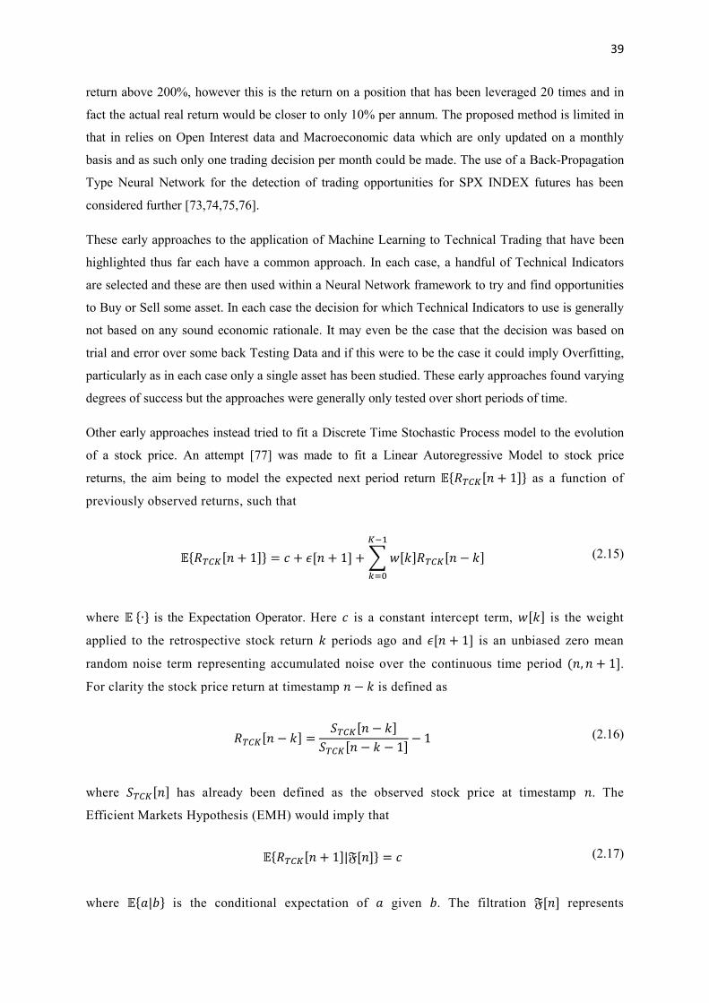
39

return above 200%, however this is the return on a position that has been leveraged 20 times and in

fact the actual real return would be closer to only 10% per annum. The proposed method is limited in

that in relies on Open Interest data and Macroeconomic data which are only updated on a monthly

basis and as such only one trading decision per month could be made. The use of a Back-Propagation

Type Neural Network for the detection of trading opportunities for SPX INDEX futures has been

considered further [73,74,75,76].

These early approaches to the application of Machine Learning to Technical Trading that have been

highlighted thus far each have a common approach. In each case, a handful of Technical Indicators

are selected and these are then used within a Neural Network framework to try and find opportunities

to Buy or Sell some asset. In each case the decision for which Technical Indicators to use is generally

not based on any sound economic rationale. It may even be the case that the decision was based on

trial and error over some back Testing Data and if this were to be the case it could imply Overfitting,

particularly as in each case only a single asset has been studied. These early approaches found varying

degrees of success but the approaches were generally only tested over short periods of time.

Other early approaches instead tried to fit a Discrete Time Stochastic Process model to the evolution

of a stock price. An attempt [77] was made to fit a Linear Autoregressive Model to stock price

returns, the aim being to model the expected next period return 𝔼{𝑅𝑇𝐶𝐾[𝑛 + 1]} as a function of

previously observed returns, such that

𝔼{𝑅𝑇𝐶𝐾[𝑛 + 1]} = 𝑐 + 𝜖[𝑛 + 1] + ∑ 𝑤[𝑘]𝑅𝑇𝐶𝐾[𝑛 − 𝑘]

𝐾−1

𝑘=0

(2.15)

where 𝔼 {∙} is the Expectation Operator. Here 𝑐 is a constant intercept term, 𝑤[𝑘] is the weight

applied to the retrospective stock return 𝑘 periods ago and 𝜖[𝑛 + 1] is an unbiased zero mean

random noise term representing accumulated noise over the continuous time period (𝑛, 𝑛 + 1].

For clarity the stock price return at timestamp 𝑛 − 𝑘 is defined as

𝑅𝑇𝐶𝐾[𝑛 − 𝑘] =𝑆𝑇𝐶𝐾[𝑛 − 𝑘]

𝑆𝑇𝐶𝐾[𝑛 − 𝑘 − 1]− 1 (2.16)

where 𝑆𝑇𝐶𝐾[𝑛] has already been defined as the observed stock price at timestamp 𝑛. The

Efficient Markets Hypothesis (EMH) would imply that

𝔼{𝑅𝑇𝐶𝐾[𝑛 + 1]|𝔉[𝑛]} = 𝑐 (2.17)

where 𝔼{𝑎|𝑏} is the conditional expectation of 𝑎 given 𝑏. The filtration 𝔉[𝑛] represents

40

knowledge of information. In the case of the Weak Form EMH, 𝔉[𝑛] would represent knowledge

of price and volume market data. In the case of the Semi Strong Form EMH, 𝔉[𝑛] would

represent knowledge of market data as well as knowledge of all publically known information.

In the case of the Strong From EMH, 𝔉[𝑛] would represent the knowledge of market data as well

as all publically and privately known information. The value 𝑐 would then represent a constant

per period drift rate that would be proportional to the risk free interest rate plus some risk

premium. A sufficient condition for the EMH to hold is 𝑤[𝑘] = 0 ∀𝑘.

The published approach [77] attempts to fit linear weights in the single hidden layer of a Neural

Network to create a mapping from 𝑅𝑇𝐶𝐾[𝑛 − 𝑘] ∀𝑘 ∈ {0, . . , 𝐾 − 1} to 𝔼{𝑅𝑇𝐶𝐾[𝑛 + 1]}. The

Neural Network is limited such that each of the 𝐾 nodes within the hidden layer is connected to

only a single input node and as such the internal weights of the hidden layer would be equivalent

to 𝑐 and 𝑤[𝑘] ∀𝑘 ∈ {0, . . , 𝐾 − 1} in Equation 2.15. The paper considered the stock price returns

of International Business Machines (Bloomberg Code: IBM EQUITY) over a time period of two

years. The paper concluded that the weights 𝑤[𝑘] ∀𝑘 ∈ {0, . . , 𝐾 − 1} fitted over some training

interval were not useful for reliable prediction of 𝑅𝑇𝐶𝐾[𝑛 + 1] over some following test period.

The restriction to linear weights was then relaxed such that 𝔼{𝑅𝑇𝐶𝐾[𝑛 + 1]} could be some non-

linear function of 𝑅𝑇𝐶𝐾[𝑛 − 𝑘] ∀𝑘 ∈ {0, . . , 𝐾 − 1}, and again the conclusion was made that the

weights 𝑤[𝑘] ∀𝑘 ∈ {0, . . , 𝐾 − 1} fitted over some training interval were not useful for reliable

prediction of 𝑅𝑇𝐶𝐾[𝑛 + 1] over some following test period. The paper concluded that

autoregressive models cannot be easily fit, although only a single stock had been considered.

Another attempt [78] at fitting an Autoregressive Model looked at including the difference and second

difference of returns into the stochastic model framework, such that the predicted next period return

𝔼{𝑅𝑇𝐶𝐾[𝑛 + 1]} is modelled as

𝔼{𝑅𝑇𝐶𝐾[𝑛 + 1]}

= 𝑐 + 𝜖[𝑛 + 1] + ∑𝑤[𝑘]𝑅𝑇𝐶𝐾[𝑛 − 𝑘]

𝐾−1

𝑘=0

+∑𝜃[𝑙]

𝐿−1

𝑙=0

(𝑅𝑇𝐶𝐾[𝑛 − 𝑙] − 𝑅𝑇𝐶𝐾[𝑛 − 𝑙 − 1])

+ ∑ 𝜑[ℎ]

𝐻−1

ℎ=0

(𝑅𝑇𝐶𝐾[𝑛 − ℎ] − 2𝑅𝑇𝐶𝐾[𝑛 − ℎ − 1] + 𝑅𝑇𝐶𝐾[𝑛 − ℎ − 2])

(2.18)

where the weights 𝜃[𝑙]∀𝑙 ∈ {0, . . , 𝐿 − 1} and 𝜑[ℎ]∀ℎ ∈ {0, . . , 𝐻 − 1} are the weights applied to the

first and second differences of the observed historical stock price returns respectively. A Neural

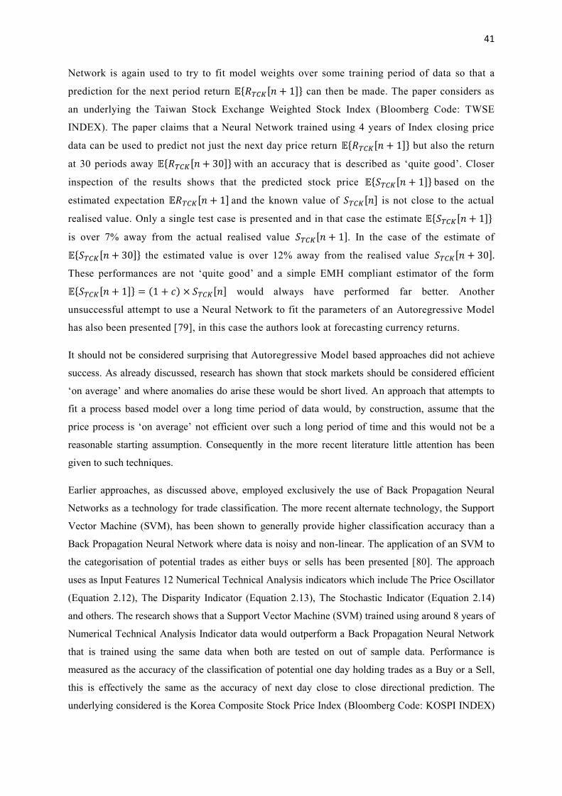
41

Network is again used to try to fit model weights over some training period of data so that a

prediction for the next period return 𝔼{𝑅𝑇𝐶𝐾[𝑛 + 1]} can then be made. The paper considers as

an underlying the Taiwan Stock Exchange Weighted Stock Index (Bloomberg Code: TWSE

INDEX). The paper claims that a Neural Network trained using 4 years of Index closing price

data can be used to predict not just the next day price return 𝔼{𝑅𝑇𝐶𝐾[𝑛 + 1]} but also the return

at 30 periods away 𝔼{𝑅𝑇𝐶𝐾[𝑛 + 30]} with an accuracy that is described as ‘quite good’. Closer

inspection of the results shows that the predicted stock price 𝔼{𝑆𝑇𝐶𝐾[𝑛 + 1]} based on the

estimated expectation 𝔼𝑅𝑇𝐶𝐾[𝑛 + 1] and the known value of 𝑆𝑇𝐶𝐾[𝑛] is not close to the actual

realised value. Only a single test case is presented and in that case the estimate 𝔼{𝑆𝑇𝐶𝐾[𝑛 + 1]}

is over 7% away from the actual realised value 𝑆𝑇𝐶𝐾[𝑛 + 1]. In the case of the estimate of

𝔼{𝑆𝑇𝐶𝐾[𝑛 + 30]} the estimated value is over 12% away from the realised value 𝑆𝑇𝐶𝐾[𝑛 + 30].

These performances are not ‘quite good’ and a simple EMH compliant estimator of the form

𝔼{𝑆𝑇𝐶𝐾[𝑛 + 1]} = (1 + 𝑐) × 𝑆𝑇𝐶𝐾[𝑛] would always have performed far better. Another

unsuccessful attempt to use a Neural Network to fit the parameters of an Autoregressive Model

has also been presented [79], in this case the authors look at forecasting currency returns.

It should not be considered surprising that Autoregressive Model based approaches did not achieve

success. As already discussed, research has shown that stock markets should be considered efficient

‘on average’ and where anomalies do arise these would be short lived. An approach that attempts to

fit a process based model over a long time period of data would, by construction, assume that the

price process is ‘on average’ not efficient over such a long period of time and this would not be a

reasonable starting assumption. Consequently in the more recent literature little attention has been

given to such techniques.

Earlier approaches, as discussed above, employed exclusively the use of Back Propagation Neural

Networks as a technology for trade classification. The more recent alternate technology, the Support

Vector Machine (SVM), has been shown to generally provide higher classification accuracy than a

Back Propagation Neural Network where data is noisy and non-linear. The application of an SVM to

the categorisation of potential trades as either buys or sells has been presented [80]. The approach

uses as Input Features 12 Numerical Technical Analysis indicators which include The Price Oscillator

(Equation 2.12), The Disparity Indicator (Equation 2.13), The Stochastic Indicator (Equation 2.14)

and others. The research shows that a Support Vector Machine (SVM) trained using around 8 years of

Numerical Technical Analysis Indicator data would outperform a Back Propagation Neural Network

that is trained using the same data when both are tested on out of sample data. Performance is

measured as the accuracy of the classification of potential one day holding trades as a Buy or a Sell,

this is effectively the same as the accuracy of next day close to close directional prediction. The

underlying considered is the Korea Composite Stock Price Index (Bloomberg Code: KOSPI INDEX)

42

and the test period represents around two years between December 1996 and December 1998 with the

actual results being published in 2003. An optimised Support Vector Machine (SVM) showed a

prediction accuracy of around 57.8% compared with an accuracy of 54.7% for an optimised Back

Propagation Neural Network, the performance difference is not large and has been shown over only a

single set of Test Data. The Back Propagation Neural Network is only one of many possible Neural

Network architectures and it is possible that other architectures may have performed better.

Although increases in computing power allow a greater number of Input Features to be used for either

a Neural Network or an SVM there exists no rationale to suggest that increasing the breadth of Input

Features would lead to an improved performance. Most human Technical Traders would have a

preferred combination of a few Technical Indicators and may use, for example, some Technical

Indicators to make an initial trading decision and other indicators to reinforce a decision. An

experienced human expert would also look to base trading decisions on a rational premise and where

a combination of Technical Indicators are used the choice of combination would typically be based on

some prevailing economic factors. An approach that may be seen as throwing a lot of technical data at

a black box would generally not be considered rational. Much of the later research then focussed

towards the processing of Input Feature data and to Input Feature selection. The general motivations

for Input Feature discretisation and feature selection are to increase prediction accuracy, to reduce

computational complexity and also to reduce the risk of overfitting of the Training Data.

General studies [81] have shown that the use of Input Feature discretisation techniques can reduce the

effective dimensionality of the Input Feature space and that this in turn can lead to an increased

accuracy of classification by Neural Networks. The aim is to reduce the dimensionality of the Input

Feature space by transforming continuous value Input Features into discretised equivalents based on

determined thresholds. An approach to Input Feature discretisation for a Neural Network for stock

direction prediction has been presented [82]. The approach considers as Input Features the same 12

Numerical Technical Analysis indicators used in [80], with each feature being discretised with

between 1 and 5 possible categories based upon 4 variable boundaries. The case of an Input Feature

being categorised to only a single possible level would correspond to that feature being effectively

made redundant and as such the proposed technique can also potentially achieve feature selection.

Genetic Algorithm (GA) techniques are used to find simultaneously the optimal feature discretisation

boundaries as well the weights of the Neural Network connections over a training period of around 8

years. The optimal solution is defined to be that which gives the highest directional prediction

accuracy over the Training Data. Over a testing period of around two years with the underlying again

being the Korea Composite Stock Price Index (Bloomberg Code: KOSPI INDEX) it is shown that the

GA optimised Neural Network with Feature Discretisation would outperform a Back Propagation

Neural Network with classification accuracies of 61.7% and 51.8% respectively. It should be noted

that of the 12 Input Features none were determined to be redundant. It should also be noted that in a

43

separate test without feature discretisation it was shown that optimising the weights of the Neural

Network connections by either GA or by Back Propagation produced similar levels of performance on

the Test Data and as such it was concluded that it was the role of GA for feature discretisation that

had produced the performance increase.

Input Feature Selection is a general term used to describe processes that are used to select the subset

of possible Input Features that are deemed most essential for classification. Input Feature Selection is

in itself a widely researched subject in a general Machine Learning context and here only a brief

overview of the subject will be presented. In summary Input Feature Selection techniques can be

divided into two broad categories, these are the so called Filter Methods [83] and the Wrapper

Methods [84]. Filter Methods estimate the relevance of an Input Feature without recourse to the

output results of a Predictor, Filter Methods are generally based on statistical tests which consider

some correlation type based measure between the value of a particular Input Feature and the

classification within a Training Set. Those Input Features that are deemed to have the strongest

statistical link to the division of classes within a Training Set are deemed the most essential for

classification. Wrapper Methods, however, do consider the optimisation of the output values of a

classifier, with the typical classifier being a Neural Network or an SVM. Wrapper Methods are

generally based on some measure of the improvement of the quality of classification for a Training

Set based on the introduction of a particular Input Feature. Whilst Wrapper Methods have been shown

to be more effective at selecting an optimal feature subset than Filter Methods, the Wrapper Methods

have a much higher degree of computational complexity.

The application of Input Feature Selection techniques for Stock Price prediction has been considered

simultaneously for both a Neural Network framework and an SVM framework [85]. The presented

approach considers the initial application of a Filter Method to create a first subset of Input Features

and the subsequent application of Wrapper Methods to determine a refined Input Feature subset. The

approach considers 30 possible Input Features, with each Input Feature being the relative position of

some asset (with 30 assets in total) within its recent trading range. The Input Feature assets considered

include other stock indices including the Dow Jones Industrial Average (Bloomberg Code: INDU

INDEX) and currencies as well as commodities. Test results are presented for the accuracy of the next

day direction prediction of the NASDAQ Index (Bloomberg Code: CCMP INDEX). The test results

show that for an SVM with an optimally selected subset of Input Features a next day directional

prediction accuracy in excess of 85% could be achieved and an accuracy of over 70% could be

achieved when using a Back Propagation Neural Network. Whilst the results appear impressive they

are flawed. The test results have been shown as an average over a 5-fold holdout cross validation, the

use of cross validation techniques would imply that training would have been carried out on

temporally forward looking data that would be as-yet unseen in practice. In addition the Input

Features are price levels that are normalised within the continuous range [0,1] with normalisation

44

requiring knowledge of the extreme values of the Input Feature range within the complete set of

Training Data. The application of such normalisation with a 5-fold cross validation would then

introduce information from the hold-out Testing Data to the Training Data. In addition it appears that

the detection of the next day direction of the NASDAQ INDEX assumes knowledge of the next day

level of each of the 30 possible Input Features and as such the method shows no real predictive power

although the method could be used to confirm a contemporaneous relationship.

Another attempt at the use of Wrapper Methods for Input Feature selection for stock market

prediction has been presented [86]. In this approach a range of more traditional Technical Analysis

Indicators form the potential Input Feature set. An optimised Input Feature subset is determined by

Wrapper Methods to give the most accurate prediction of the next day level of the Shanghai

Composite Index (Bloomberg Code: SHCOMP INDEX) over a Training Data set that spans just two

months of market data. Testing result show the prediction of a forward level for each of the 10

business days that follow the training period. The testing results do look impressive in terms of the

absolute distance of the predicted future index level from the later realised level. However the

practical application of such day by day future predicted index levels would almost certainly be to

make directional trades and for the 10 business days for which testing results are presented the

implied direction prediction would only have been correct for just 5 out of the 10 days considered.

However, it would not be possible to draw any real conclusions with such a limited set of Test Data.

A more thorough testing across more than one short realisation of data would have been useful in

order to demonstrate the true effectiveness of the proposed method.

The review of the current literature has shown that there is room for improvement from the current

methods. Any method that does not rely upon throwing a large breadth of Technical Analysis

indicator data at a Neural Network or an SVM but instead is based on just a few tractable indicators

with a clear economic rationale would be preferred. In addition the real world effect of Transaction

Costs should be considered. The focus of the literature has generally been towards maximising the

accuracy of next day direction prediction and any new method should instead focus towards the

generation of trading profits as the purpose of trading is generally to make money.

2.4 Portfolio Construction

In this section a review of the current state of the art of methods for Portfolio Construction is

presented. Having determined a set of potential tradable assets, using for example one of the

techniques discussed in the previous section, a combination of these assets needs to be selected to

form a trading Portfolio. The weighted selection of assets into a diversified Portfolio is a complex

optimisation problem which has been approached in both the Frequentist and Bayesian frameworks.

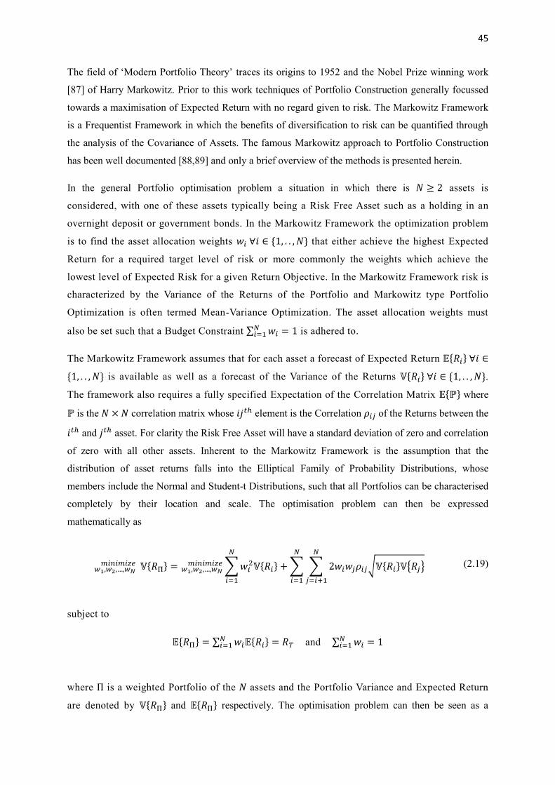
45

The field of ‘Modern Portfolio Theory’ traces its origins to 1952 and the Nobel Prize winning work

[87] of Harry Markowitz. Prior to this work techniques of Portfolio Construction generally focussed

towards a maximisation of Expected Return with no regard given to risk. The Markowitz Framework

is a Frequentist Framework in which the benefits of diversification to risk can be quantified through

the analysis of the Covariance of Assets. The famous Markowitz approach to Portfolio Construction

has been well documented [88,89] and only a brief overview of the methods is presented herein.

In the general Portfolio optimisation problem a situation in which there is 𝑁 ≥ 2 assets is

considered, with one of these assets typically being a Risk Free Asset such as a holding in an

overnight deposit or government bonds. In the Markowitz Framework the optimization problem

is to find the asset allocation weights 𝑤𝑖 ∀𝑖 ∈ {1, . . , 𝑁} that either achieve the highest Expected

Return for a required target level of risk or more commonly the weights which achieve the

lowest level of Expected Risk for a given Return Objective. In the Markowitz Framework risk is

characterized by the Variance of the Returns of the Portfolio and Markowitz type Portfolio

Optimization is often termed Mean-Variance Optimization. The asset allocation weights must

also be set such that a Budget Constraint ∑ 𝑤𝑖𝑁𝑖=1 = 1 is adhered to.

The Markowitz Framework assumes that for each asset a forecast of Expected Return 𝔼{𝑅𝑖} ∀𝑖 ∈

{1, . . , 𝑁} is available as well as a forecast of the Variance of the Returns 𝕍{𝑅𝑖} ∀𝑖 ∈ {1, . . , 𝑁}.

The framework also requires a fully specified Expectation of the Correlation Matrix 𝔼{ℙ} where

ℙ is the 𝑁 × 𝑁 correlation matrix whose 𝑖𝑗𝑡ℎ element is the Correlation 𝜌𝑖𝑗 of the Returns between the

𝑖𝑡ℎ and 𝑗𝑡ℎ asset. For clarity the Risk Free Asset will have a standard deviation of zero and correlation

of zero with all other assets. Inherent to the Markowitz Framework is the assumption that the

distribution of asset returns falls into the Elliptical Family of Probability Distributions, whose

members include the Normal and Student-t Distributions, such that all Portfolios can be characterised

completely by their location and scale. The optimisation problem can then be expressed

mathematically as

𝕍{𝑅Π} =𝑤1,𝑤2,…,𝑤𝑁𝑚𝑖𝑛𝑖𝑚𝑖𝑧𝑒 ∑𝑤𝑖

2𝕍{𝑅𝑖}

𝑁

𝑖=1

+∑ ∑ 2𝑤𝑖𝑤𝑗𝜌𝑖𝑗√𝕍{𝑅𝑖}𝕍{𝑅𝑗}

𝑁

𝑗=𝑖+1

𝑁

𝑖=1

𝑤1,𝑤2,…,𝑤𝑁𝑚𝑖𝑛𝑖𝑚𝑖𝑧𝑒 (2.19)

subject to

𝔼{𝑅Π} = ∑ 𝑤𝑖𝔼{𝑅𝑖}𝑁𝑖=1 = 𝑅𝑇 and ∑ 𝑤𝑖

𝑁𝑖=1 = 1

where Π is a weighted Portfolio of the 𝑁 assets and the Portfolio Variance and Expected Return

are denoted by 𝕍{𝑅Π} and 𝔼{𝑅Π} respectively. The optimisation problem can then be seen as a

46

minimisation of Portfolio Variance to achieve some target Return Objective 𝑅𝑇 subject to a Budget

Constraint that no more and no less than 100% of the available capital is invested into the 𝑁

assets which include the Risk Free Asset. The format of Equation 2.19 demonstrates the effect of

diversification whereby increasing the number of assets 𝑁 leads to a lowering of Portfolio

Variance. The convex optimisation problem of Equation 2.19, subject to the stated equality

constraints, can be solved analytically by the Lagrange Method [90].

The solution of the optimisation problems will yield weights such that −∞ ≤ 𝑤𝑖 ≤ ∞ ∀𝑖 ∈

{1, . . , 𝑁} and hence both short selling and leverage could be introduced into the optimized

Portfolio. An additional set of inequality constraints of the form 𝑤𝑖 ≥ 0 ∀𝑖 ∈ {1, . . , 𝑁} could be

introduced to eliminate short selling and leverage. The extended optimization problem, subject

to the two equality constraints and the new inequality constraints, would require formulation of a

Karush–Kuhn–Tucker (KKT) system of equations [38] and a Numerical Non-Linear

Programming Method [91] would be needed to find a solution.

An alternative formulation of the optimization problem is as a Utility Maximization problem

[92]. Here the objective is to find the asset allocation weights 𝑤𝑖∀𝑖 ∈ {1, . . , 𝑁} which maximize

the Quadratic Utility of the Portfolio. The problem can be expressed mathematically as

𝔼{𝑅Π} −𝜆

2𝕍{𝑅Π} =𝑤1,𝑤2,…,𝑤𝑁

𝑚𝑎𝑥𝑖𝑚𝑖𝑧𝑒 ∑𝑤𝑖𝔼{𝑅𝑖}

𝑁

𝑖=1

−𝜆

2∙ (∑𝑤𝑖

2𝕍{𝑅𝑖}

𝑁

𝑖=1

+∑ ∑ 2𝑤𝑖𝑤𝑗𝜌𝑖𝑗√𝕍{𝑅𝑖}𝕍{𝑅𝑗}

𝑁

𝑗=𝑖+1

𝑁

𝑖=1

)𝑤1,𝑤2,…,𝑤𝑁

𝑚𝑎𝑥𝑖𝑚𝑖𝑧𝑒 (2.20)

subject to

∑ 𝑤𝑖𝑁𝑖=1 = 1 and 𝑤𝑖 ≥ 0 ∀𝑖 ∈ {1, . . , 𝑁}

where 𝜆 is a subjective input parameter termed “The Degree of Risk Aversion” and is used to control

the degree of maximisation of Expected Portfolio Return against the minimisation of Portfolio

Variance. The solution of such a problem again requires the use of numerical optimisation techniques.

Alternative formulations for the Objective Function are to Maximise the Sharpe Ratio [93], such that

the Optimisation Problem can be specified as

𝔼{𝑅Π} − 𝑟

√𝕍{𝑅Π}=𝑤1,𝑤2,…,𝑤𝑁

𝑚𝑎𝑥𝑖𝑚𝑖𝑧𝑒 ∑ 𝑤𝑖𝔼{𝑅𝑖}𝑁𝑖=1 − 𝑟

√(∑ 𝑤𝑖2𝕍{𝑅𝑖}

𝑁𝑖=1 + ∑ ∑ 2𝑤𝑖𝑤𝑗𝜌𝑖𝑗√𝕍{𝑅𝑖}𝕍{𝑅𝑗}

𝑁𝑗=𝑖+1

𝑁𝑖=1 )

𝑤1,𝑤2,…,𝑤𝑁

𝑚𝑎𝑥𝑖𝑚𝑖𝑧𝑒 (2.21)

subject to

∑ 𝑤𝑖𝑁𝑖=1 = 1 and 𝑤𝑖 ≥ 0 ∀𝑖 ∈ {1, . . , 𝑁}

where 𝑟 is the risk free rate. The Optimisation Problem is to then to Maximise the Risk Weighted

Excess Return of the Portfolio, where Excess Return is defined with respect to the risk free rate. In the

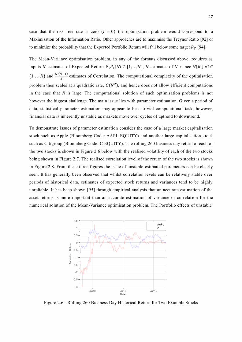
47

case that the risk free rate is zero (𝑟 = 0) the optimisation problem would correspond to a

Maximisation of the Information Ratio. Other approaches are to maximise the Treynor Ratio [92] or

to minimize the probability that the Expected Portfolio Return will fall below some target 𝑅𝑇 [94].

The Mean-Variance optimisation problem, in any of the formats discussed above, requires as

inputs 𝑁 estimates of Expected Return 𝔼{𝑅𝑖} ∀𝑖 ∈ {1, . . , 𝑁}, 𝑁 estimates of Variance 𝕍{𝑅𝑖} ∀𝑖 ∈

{1, . . , 𝑁} and 𝑁∙(𝑁−1)

2 estimates of Correlation. The computational complexity of the optimisation

problem then scales at a quadratic rate, 𝑂(𝑁2), and hence does not allow efficient computations

in the case that 𝑁 is large. The computational solution of such optimisation problems is not

however the biggest challenge. The main issue lies with parameter estimation. Given a period of

data, statistical parameter estimation may appear to be a trivial computational task; however,

financial data is inherently unstable as markets move over cycles of uptrend to downtrend.

To demonstrate issues of parameter estimation consider the case of a large market capitalisation

stock such as Apple (Bloomberg Code: AAPL EQUITY) and another large capitalisation s tock

such as Citigroup (Bloomberg Code: C EQUITY). The rolling 260 business day return of each of

the two stocks is shown in Figure 2.6 below with the realised volatility of each of the two stocks

being shown in Figure 2.7. The realised correlation level of the return of the two stocks is shown

in Figure 2.8. From these three figures the issue of unstable estimated parameters can be clearly

seen. It has generally been observed that whilst correlation levels can be relatively stable over

periods of historical data, estimates of expected stock returns and variances tend to be highly

unreliable. It has been shown [95] through empirical analysis that an accurate estimation of the

asset returns is more important than an accurate estimation of variance or correlat ion for the

numerical solution of the Mean-Variance optimisation problem. The Portfolio effects of unstable

Figure 2.6 - Rolling 260 Business Day Historical Return for Two Example Stocks

Jan10 Jul12 Jan15

-3

-2.5

-2

-1.5

-1

-0.5

0

0.5

1

1.5

Date

Annualis

ed R

etu

rn

AAPL

C

48

Figure 2.7 – Rolling 260 Business Day Realized Volatility for Two Example Stocks

Figure 2.8 – Rolling 260 Business Day Realized Correlation for Two Example Stocks

Figure 2.9 - Percentage of Portfolio Invested into One Stock with Mean-Variance Optimization

Jan10 Jul12 Jan15

0

0.2

0.4

0.6

0.8

1

1.2

1.4

1.6

1.8

Date

Annualis

ed V

ola

tilit

y

AAPL

C

Jan10 Jul12 Jan15

0

0.1

0.2

0.3

0.4

0.5

0.6

0.7

Date

Realis

ed C

orr

ela

tion

Corr AAPL/C

Jan10 Jul12 Jan15

0

0.1

0.2

0.3

0.4

0.5

0.6

0.7

0.8

0.9

1

Date

% W

eig

ht

AA

PL

% Weight AAPL

49

parameters is demonstrated in Figure 2.9, here the percentage of the Portfolio that is invested

into Apple is shown on a day by day basis. Figure 2.9 is generated for a daily Sharpe Ratio

(Equation 2.21) re-optimisation of a three asset Portfolio with the assets being Apple, Citigroup

and a Risk Free Asset which is earning zero interest. Portfolio optimisation based on unstable

parameters that are determined in a Frequentist Framework is clearly problematic. A continual

rebalancing of the Portfolio, as shown in Figure 2.9, would lead to a high level of Transaction

Costs and would also not give an investor confidence.

The issue of the accurate estimation of Expected Return of an asset had initially been addressed

through the Capital Asset Pricing Model (CAPM) whereby the Expected Return of the 𝑖𝑡ℎ asset

𝔼{𝑅𝑖} ∀𝑖 ∈ {1, . . , 𝑁} is linked linearly to the Expected Return of a Reference Asset 𝔼{𝑅𝑀} which

is typically a Market Index. The CAPM is a single parameter model and the single coefficient

𝛽𝑖∀𝑖 ∈ {1, . . , 𝑁} is typically estimated through an Ordinary Least Squares (OLS) regression

based on historical data. It can be shown [11] that the OLS solution of the Parameter 𝛽𝑖 is

𝛽𝑖 = 𝜌𝑖𝑀 .𝕍{𝑅𝑖}

𝕍{𝑅𝑀}, where 𝕍{𝑅𝑀} is the Variance of the Market Index and 𝜌𝑖𝑀 is the correlation of the

returns of the Market Index with the 𝑖𝑡ℎ asset. The issue of the estimation of the Expected Return

of the 𝑖𝑡ℎ asset 𝔼{𝑅𝑖} ∀𝑖 ∈ {1, . . , 𝑁} then becomes an issue of the estimation of the Expected

Return 𝔼{𝑅𝑀} of a single market index and the estimation of Variance and Correlation levels

which are in any case needed for the Mean-Variance Portfolio Optimization problem. Although

the CAPM model is widely used, empirical evidence [96,97] has shown that the model is

simplistic and generally achieves poor performance. Multifactor models whereby 𝔼{𝑅𝑖} ∀𝑖 ∈

{1, . . , 𝑁} is modelled as a linear function of several factors have also received consideration in

the literature [98], the factors may include the Expectation of the Return of the Market Index

𝔼{𝑅𝑀} as well as other factors such as Interest Rates and the GDP. However, studies [99] have

shown that multifactor models offer little performance improvement over the CAPM model .

Historical data approaches to Parameter Estimation are based on purely historic data and do not

allow an incorporation of other data sources. In a predictive trading framework, using for

example one of the Neural Network methods discussed above, additional information in terms of

an estimate of the next period Expected Return may be available. Such additional information

could be used to adjust an initial forecast based upon historical data. The Black-Litterman Model

[100] is a Bayesian Framework which allows an initial forecast of Expected Return to be

updated based on later observed data. The Black-Litterman approach can be summarized in

terms of Bayes formula

𝑃(𝐸|𝐼) =𝑃(𝐼|𝐸)

𝑃(𝐼)𝑃(𝐸) (2.22)

50

where 𝑃(𝐸) is the prior joint probability distribution of the Expected Excess Returns of the 𝑁 assets

where Excess is with respect to a Risk Free Asset with return 𝑟. In the Black-Litterman model it is

assumed that 𝑃(𝐸) follows a Multivariate Normal Distribution where the prior Means and

Covariances of the Expected Excess Returns can be based upon historical data. It is more typical for

the prior Means to be implied from a backward solution of the Utility Function (Equation 2.20) under

the assumption that the initial asset allocation weights 𝑤𝑖∀𝑖 ∈ {1, . . , 𝑁} are based upon the relative

asset weights in a Market Portfolio, this is to imply that the starting assumption is that The

Efficient Markets Hypothesis (EMH) holds and that the optimal starting Portfolio is the Market

Portfolio. The prior Covariance Matrix used to model the distribution of the Expected Excess

Returns 𝑃(𝐸) is typically based upon a scalar multiple of the Covariance Matrix of the Historical

Excess Returns where the subjective Scaling Factor Level is typically between 0.01 and 0.05. Within

the Black-Litterman Framework a joint Normal Distribution 𝑃(𝐼) of ‘views’ on the 𝑁 assets can be

incorporated, such a distribution is parameterized in terms of the Mean Views and Confidence of

Views. The Mean Views used to form 𝑃(𝐼) may be based upon a Neural Network method such as

those discussed in the previous subsection. The formation of a vector of the confidence of the views

introduces another parameter estimation issue into the optimisation problem.

The Black-Litterman framework is based upon joint Normal Distributions. However, empirical

evidence has suggested that asset price returns are not Normally Distributed and that excess kurtosis

exists. It has been suggested [101] that excess kurtosis is created as an effect of volatility clustering

whereby large price changes tend to be followed by large price changes, of either positive or negative

sign, and smaller price changes tend to be followed by similar small price changes. This is to suggest

that price returns are generated by a mixture of Normal Distributions and the resulting distribution

then has a kurtosis that is greater than three [102]. It is this idea of a mixture of Normal Distributions

that has led to the consideration of the Student-t distribution, the Generalised Hyperbolic Distribution

and the Variance-Gamma distribution for the modelling of asset price returns. Methods for improved

estimates of the Variance of the Returns 𝕍{𝑅𝑖} ∀𝑖 ∈ {1, . . , 𝑁} have also been proposed. Such

methods include the use of Autoregressive ARCH Models [102].

This review of the current literature has shown that there is room for improvement from the current

methods for Portfolio Construction. Standard Portfolio Construction techniques in the Mean-Variance

optimisation framework have been shown to be highly sensitive to the estimated values of input

parameters. It has been shown that the estimation of such input parameters in a simplistic Frequentist

Framework leads to unstable estimates which in turn generally give unstable Portfolios. Later research

then focussed to address the issues of parameter estimation and adaptive Bayesian methods such as

The Black-Litterman method had received some attention. This Bayesian approach is however seen to

be limited in that it places a strong distributional assumption upon the form of data.

51

In a trading strategy where trading decisions are based upon a Neural Network output, such as one of

the methods illustrated in the previous section, it may not be reasonable to assume that the returns of a

single asset are well modelled by a particular distribution. As such, any new method that is

particularly geared towards Portfolio Construction in an environment where trading opportunities are

detected by a Neural Network method should ideally be free of distribution assumptions and should

also simultaneously address issues caused by parameter instability.

2.5 Order Entry Timing: Market Order Book and Order Execution

In this section a review of the current state of the art of methods for Market Order Book modelling

and Order Execution techniques is presented. Having determined a set of potential tradable assets and

their weights in a Portfolio all that remains is to execute trades and form the actual monetised

Portfolio. Stocks are commonly traded over electronic exchanges using a Continuous Double Auction

Based Limit Order Book and in this section a number of state of the art techniques of modelling such

an Order Book are presented. The Chapter aims to shows that whilst such techniques are well suited

to Electronic Market Making they are not well suited to Order Execution where there is a requirement

for one hundred percent order completion.

An example Double Auction Based Limit Order Book for General Electric (Bloomberg Code: GE

EQUITY) from multiple trading venues is shown below in Figure 2.10. The Limit Order Book

consists of a Queue of Buyers (Bid Side Queue) who have placed limit orders to Buy shares of GE up

to specified price limits. In addition there is a Queue of Sellers (Offer Side Queue) who have placed

limit orders to Sell shares of GE down to specified price limits.

Figure 2.10 – Example Double Auction Based Limit Order Book for General Electric

52

The Bid Side Queue 𝐵[𝑡] at a discrete timestamp 𝑡 can be represented by a 𝑘 dimensional vector of

tuples where the 𝑖th entry is {𝑄−𝑖, 𝑞−𝑖}, where the subscript −𝑖 refers to this being the 𝑖th tick on the

left side (Bid Side) of the order book, 𝑄−𝑖 is the price at this 𝑖th tick and 𝑞−𝑖 is the quantity available

at this tick. The Bid Side Queue can then be represented as

𝐵[𝑡] = [{𝑄−1, 𝑞−1}, {𝑄−2, 𝑞−2},… , {𝑄−(𝑘−1), 𝑞−(𝑘−1)}, {𝑄−𝑘, 𝑞−𝑘}] (2.23)

The Offer Side Queue 𝐴[𝑡] at a discrete timestamp 𝑡 can also be represented by a 𝑘 dimensional

vector of tuples where the 𝑖th entry is {𝑄𝑖, 𝑞𝑖}, where the subscript 𝑖 refers to this being the 𝑖th tick on

the right side (Offer or Ask Side) of the order book, 𝑄𝑖 is the price at this 𝑖th tick and 𝑞𝑖 is the

quantity available at this tick. The Offer (Ask) Side Queue can then be represented as

𝐴[𝑡] = [{𝑄1, 𝑞1}, {𝑄2, 𝑞2},… , {𝑄𝑘−1, 𝑞𝑘−1}, {𝑄𝑘, 𝑞𝑘}] (2.24)

The Bid Side Queue for the Example Order Book shown in Figure 2.10 can be represented as

𝐵[𝑡] = [{30.00,73780}, {29.99,40250}, {29.98,34000}, {29.97,30660}, {29.96,25000}… ] (2.25)

The Offer Side Queue for the Example Order Book shown in Figure 2.10 can be represented as

𝐴[𝑡] = [{30.01,28000}, {30.02,34000}, {30.03,39000}, {30.04,37000}, {30.05,49000}… ] (2.26)

General Electric has shares available at the five nearest ticks on both sides of the order book. The

order book for Cimarex Energy (Bloomberg Code: XEC EQUITY) is shown below.

Figure 2.11 – Example Double Auction Based Limit Order Book for Cimarex Energy

53

From Figure 2.11 it can be seen that there is a gap between the Best Bid (92.11) and the Best Offer

(92.56). The Bid Side Queue for the Example Order Book shown in Figure 2.11 can be represented as

𝐵[𝑡] = [… {92.11,2000}, {92.10,1000}, {92.09,0}, {92.08,0}, {92.07,0}… ] (2.27)

The Offer Side Queue for the Example Order Book shown in Figure 2.11 can be represented as

𝐴[𝑡] = [… {92.56,20000}, {92.55,0}, {92.54,0}, {92.53,0}, {92.52,0}… ] (2.28)

In the case of Cimarex Energy the order book (considering just the first few ticks as above) is sparse

in the sense that there is zero tradable volume available at many ticks of the order book.

A trader wishing to execute an order has two choices; they can place a Market Order which will

execute the order at the best possible level. For example a Market Order to Buy 50000 shares of GE

based on the order book in Figure 2.10 will result in 28000 shares being purchased at the best offer

price of 30.01 and the remaining 22000 shares will be purchased at the next best offer of 30.02, the

average execution price would then be 30.014. Alternatively a trader may place a limit order. For

example a Limit Order to Buy 50000 shares of GE at 30.01 based on the order book in Figure 2.8 will

result in 28000 shares being purchased at a price of 30.01, the remaining 22000 shares would then be

queued on the Bid Side of the order book at a price of 30.01, the resulting order book assuming no

other changes would then be such that

𝐵[𝑡] = [{30.01,22000}, {30.00,73780}, {29.99,40250}, {29.98,34000}, {29.97,30660},… ] (2.29)

𝐴[𝑡] = [{30.02,34000}, {30.03,39000}, {30.04,37000}, {30.05,49000}… ] (2.30)

In the example above the limit order to Buy was placed at the level of the Best Offer, this does not

have to be case. It is possible for a patient trader to place a Buy order at some level lower down the

order book. However, common sense would suggest that the probability of execution is inversely

proportional to the initial distance of the order limit and the centre level of the order book. A trader

may wish to know the probability of an order that is placed at a certain limit price being executed or

they may wish to decide between placing a Limit Order or an order to execute at the current best bid

or offer (a Market Order). The answer to such questions is commonly determined by reference to a

model of the Market Order Book.

Simpler approaches [103,104] to the Modelling of the Limit Order Book assume that Market Orders

(to trade at Best Bid or Best Offer) and Limit Orders at each available order book price are driven by

Independent Poisson Processes where the arriving order size is a fixed number of shares. At the same

time Order Cancellation processes that remove orders from the various limit steps of the Order Book

also arrive at times driven by Independent Poisson Processes. This is to say that in Equation 2.23 and

54

Equation 2.24 each of the 𝑞𝑖 in {𝑄𝑖, 𝑞𝑖} ∀𝑖 ∈ {−𝑘,−𝑘 − 1,… ,−1,1,… , 𝑘 − 1, 𝑘} are incremented and

decremented in fixed sized steps with the times of such increments or decrements being driven by

Independent Poisson Processes. The Poisson Processes arrival rates may be set to be decreasing

functions of the absolute distance |𝑖| of a limit price from the centre of the order book to capture the

empirical observation that orders are generally placed closer to the centre of the order book. Such

models can be represented by a set of 2𝑘 Independent Markov Networks and the Learning Task (TSK)

then focusses on estimating the Transition Probabilities within each of the Independent Markov

Networks. The estimation of Transition Probabilities is typically carried out in a Frequentist setting

using observed market data over some historic period of time. After calibration these models can be

used under simulation to show a number of conclusions which may appear as obvious. For example, it

can be shown that the probability of execution is inversely proportional to the distance of the order

price from the centre of the order book and also that the probability of order cancellation is directly

proportional to the distance of the order price from the centre of the order book. It can also be shown

[105] that the order book as represented by Equation 2.23 and Equation 2.24 will converge to a

Stationary Probability Distribution of orders around a static central order book price.

The assumption of Independent Markov Networks is a clear departure from reality as it can be

empirically observed that increasing quantities at those ticks closer to the centre of the order book will

lead to an increased probability of Market Orders being placed and a decreased probability of order

cancellation. The independence assumption has been relaxed in a later approach [106] where the

Markov Transition Probabilities for order placement and cancellation are faded as the size of queued

orders increases. The model can again be shown over time to converge to a Stationary Probability

Distribution of orders around a static central price. Market Order Book models such as these are not

well suited to modelling incomplete order books such as that shown above for Cimarex Energy.

It has been shown [107] that Market Order Books are open to manipulation as orders are placed and

withdrawn by traders who do so to create the appearance of stock price activity; as such the order

book which is being modelled may not be representative of the real tradable order book. Empirical

evidence [108] also shows that Market Order Book models often do not support the true behaviour of

order books. It has also been shown [109] that placing limit orders effectively provides free

optionality to the market and should therefore be avoided. In addition the only way to ensure one

hundred percent order completion is by placing Market Orders rather than by placing limit orders

which may never be executed.

The focus of Market Order Book methods should then be towards determining the optimal timing to

place a Market Order and for this there is room for the incorporation of adaptive methods such as

Online Learning in order to have algorithms that adapt quickly to changing market conditions.

55

2.6 Summary

In this Chapter the three facets of Trading Opportunity Detection, Portfolio Construction and Order

Entry Timing have been reviewed in turn.

A number of attempts have been made to apply Neural Networks and Support Vector Machines to the

task of Trading Opportunity Detection at the level of a single asset. The approaches have varied over

time in terms of the optimisation of the Machine Learning technology that has been employed,

however the core theme has remained constant. This core theme is to throw a number of Technical

Analysis indicators at a Machine Learning technology in an attempt to find reproducible market

behaviour that can later be exploited for profit. The success of such techniques as shown in the

published literature has been underwhelming and there has been little to show that such techniques

could give sustained performance across a range of market conditions. Methods that form the current

state of the art are not grounded upon economic rationality and the focus is generally on the accuracy

of next day direction prediction and not upon the maximisation of trading profits. In Chapter 3 an

alternative Neural Network approach to Trading Opportunity Detection is presented, the method is

based on economic rationality and profit maximisation and it is shown that a sustained positive

performance can be maintained across a range of market conditions.

The current state of the art of techniques for Portfolio Construction is still grounded in the Mean-

Variance optimisation framework of Harry Markowitz. It has been shown that Portfolio Optimisation

in this framework is particularly sensitive to the quality of the estimation of the underlying statistical

parameters and recent research has focussed towards addressing the estimation issue. The estimation

of statistical parameters has been considered through Frequentist techniques and also through

Bayesian techniques such as the Black-Litterman Model. These methods all make the assumption

that Asset Returns have a distribution that falls into the Elliptical Family and as such are not

well suited for the construction of Portfolios that are based upon assets selected because they are

believed to have a distribution of returns which exhibit excess Kurtosis. Mean-Variance based

techniques are also not well suited to the construction of a dynamic Portfolio in which assets are

only held for a short period of time. In Chapter 4 a novel Bayesian Graphical Model Framework

for Dynamic Portfolio Construction is presented.

Methods for Order Entry Timing are currently based upon simulation models of the Market Order

Book and the consideration of Limit Orders and Market Orders. However research has shown that

Market Order Book models often lack accuracy. Where it is the case that one hundred percent order

completion is required a method for the timing of the placement of Market Orders is required. In

Chapter 5 it is shown how Online Learning techniques can be used to determine a more optimal

timing for the placement of Market Orders into the Trading Book.

56

Chapter 3

A New Neural Network Framework For Profitable Long-

Short Equity Trading

In this Chapter the development of a novel framework for detecting trading opportunities for single

stocks is presented. The Chapter begins with an Introduction to highlight the motivation behind the

development of the framework. The Introduction is followed by the presentation of a novel method for

detecting trading opportunities that does not rely on any advanced Machine Learning based

technologies. The first application of a Neural Network approach is then presented and this is

followed in turn by an improved Neural Network approach. As is common with Neural Network

frameworks there are a number of subjective variable parameters and a risk based approach to

optimise these parameters is then presented. Back testing results are presented to demonstrate the

performance of the proposed framework. The Chapter ends with a summary.

3.1 Introduction

In the previous Chapter a number of Machine Learning based methods for detecting trading

opportunities were presented from the wider literature. These methods typically rely on the use of

several Technical Analysis indicators with little consideration being given to the relevance of the

input data. The approach too often is to throw a lot of input data at either a Neural Network or a

Support Vector Machine and to allow the classifier to find structure within the Input Features,

otherwise optimisation techniques are used to choose amongst the available Technical Analysis

Indicators. Such approaches have little real world basis, a successful human expert trader would not

place real money at risk without a sound rational basis to trade. The method presented in this Chapter

uses a novel framework of just two Technical Analysis indicators and the development of the method

shows that a tractable basis is maintained throughout. This is important as an approach that is based

upon a sound economic rationale is an approach that would be expected to have longevity.

Current methods are mainly geared either towards estimating the future direction of price movement

over some time period or in estimating the future price level itself. The aim is typically to make a

decision to either Buy or Sell some stock or index and the number of generated trades could be large

with many methods making one Buy or Sell type trading decision per day. Studies of the Efficient

Markets Hypothesis (EMH) have shown that markets should be considered efficient on the average

with Momentum and Overreaction anomalies being possible. This would imply that at most times an

asset should be considered fairly priced and as such no trade should be placed. The novel method

57

presented in this Chapter follows from this logic and indeed rather than searching for Buy and Sell

opportunities the method instead searches directly for Momentum and Overreaction Anomalies.

Methods that form the current state of the art typically also ignore the presence of Transaction Costs

and these would deteriorate performance with a particularly substantial negative effect in the case of

methods that advocate trading on a daily basis. The novel method presented herein takes into

consideration the effect of Transaction Costs. In addition current methods are typically optimised to

maximise the probability of successful directional estimation. The novel method presented in this

Chapter is instead optimised to maximise the Risk Weighted Return. It is not uncommon for

successful expert traders to use a model with a directional accuracy prediction of less than 50% and in

the same vain the focus of the presented methods is not to maximise such accuracy. It is Return that

matters as this would translate to the generation of profits and more explicitly it is Risk Weighted

Return that should be optimised as achieving high returns should not require taking a disproportionate

amount of risk. Implementation of the methods is carried out in MATLAB and testing is conducted

across a wide range of stocks listed in the USA.

3.2 A Novel Method for Trend Detection Without Machine Learning

In this section a novel method for Trend Detection that does not require the application of

advanced Machine Learning methods is presented. This section is important as the method

developed here is later applied within a Neural Network framework. Too often the techniques

presented in the literature utilise a selection of Technical Indicators with no explanation of the

reasoning behind the choice of indicators, this section serves to explain the economic basis of

the Input Features that will be applied later within a Machine Learning framework.

At the core of the method is the direct detection of Momentum and Overreaction Anomalies.

Rather than using a wide selection of Technical Analysis indicators, a compact representation of

the market trend over some time period can be achieved through just two metrics, a Short Term

Efficiency Level and an Average Efficiency Level. The restriction to two metrics allows easy

visualization of the trade frontiers and allows a tractable basis to be maintained. The Efficiency

Indicator is similar to that from Kaufman [110] and is otherwise termed The Generalised Fractal

Efficiency. Start by assuming that market data has been regularly sampled with, for some stock

with Ticker Symbol 𝑇𝐶𝐾, the stock closing price at the 𝑛th time sample being represented as

𝑆𝑇𝐶𝐾[𝑛]. The Short Term Efficiency Level 𝛾𝑇𝐶𝐾[𝑛] at timestamp 𝑛 can then be defined as

𝛾𝑇𝐶𝐾[𝑛] =|𝑆𝑇𝐶𝐾[𝑛] − 𝑆𝑇𝐶𝐾[𝑛 − 𝐾]|

∑ |𝑆𝑇𝐶𝐾[𝑛 − 𝑘] − 𝑆𝑇𝐶𝐾[𝑛 − 𝑘 − 1]|𝐾−1𝑘=0

(3.1)

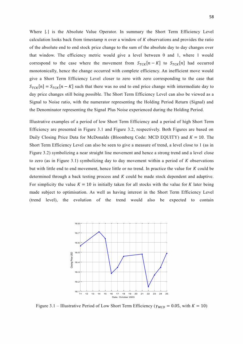
58

Where |. | is the Absolute Value Operator. In summary the Short Term Efficiency Level

calculation looks back from timestamp 𝑛 over a window of 𝐾 observations and provides the ratio

of the absolute end to end stock price change to the sum of the absolute day to day changes over

that window. The efficiency metric would give a level between 0 and 1, where 1 would

correspond to the case where the movement from 𝑆𝑇𝐶𝐾[𝑛 − 𝐾] to 𝑆𝑇𝐶𝐾[𝑛] had occurred

monotonically, hence the change occurred with complete efficiency. An inefficient move would

give a Short Term Efficiency Level closer to zero with zero corresponding to the case that

𝑆𝑇𝐶𝐾[𝑛] = 𝑆𝑇𝐶𝐾[𝑛 − 𝐾] such that there was no end to end price change with intermediate day to

day price changes still being possible. The Short Term Efficiency Level can also be viewed as a

Signal to Noise ratio, with the numerator representing the Holding Period Return (Signal) and

the Denominator representing the Signal Plus Noise experienced during the Holding Period.

Illustrative examples of a period of low Short Term Efficiency and a period of high Short Term

Efficiency are presented in Figure 3.1 and Figure 3.2, respectively. Both Figures are based on

Daily Closing Price Data for McDonalds (Bloomberg Code: MCD EQUITY) and 𝐾 = 10. The

Short Term Efficiency Level can also be seen to give a measure of trend, a level close to 1 (as in

Figure 3.2) symbolizing a near straight line movement and hence a strong trend and a level close

to zero (as in Figure 3.1) symbolizing day to day movement within a period of 𝐾 observations

but with little end to end movement, hence little or no trend. In practice the value for 𝐾 could be

determined through a back testing process and 𝐾 could be made stock dependent and adaptive.

For simplicity the value 𝐾 = 10 is initially taken for all stocks with the value for 𝐾 later being

made subject to optimisation. As well as having interest in the Short Term Efficiency Level

(trend level), the evolution of the trend would also be expected to contain

Figure 3.1 – Illustrative Period of Low Short Term Efficiency (𝛾𝑀𝐶𝐷 = 0.05, with 𝐾 = 10)

11 12 13 14 15 16 17 18 19 20 21 22 23 24 2518.1

18.2

18.3

18.4

18.5

18.6

18.7

18.8

Date. October 2003

Clo

sing

Pric

e U

SD

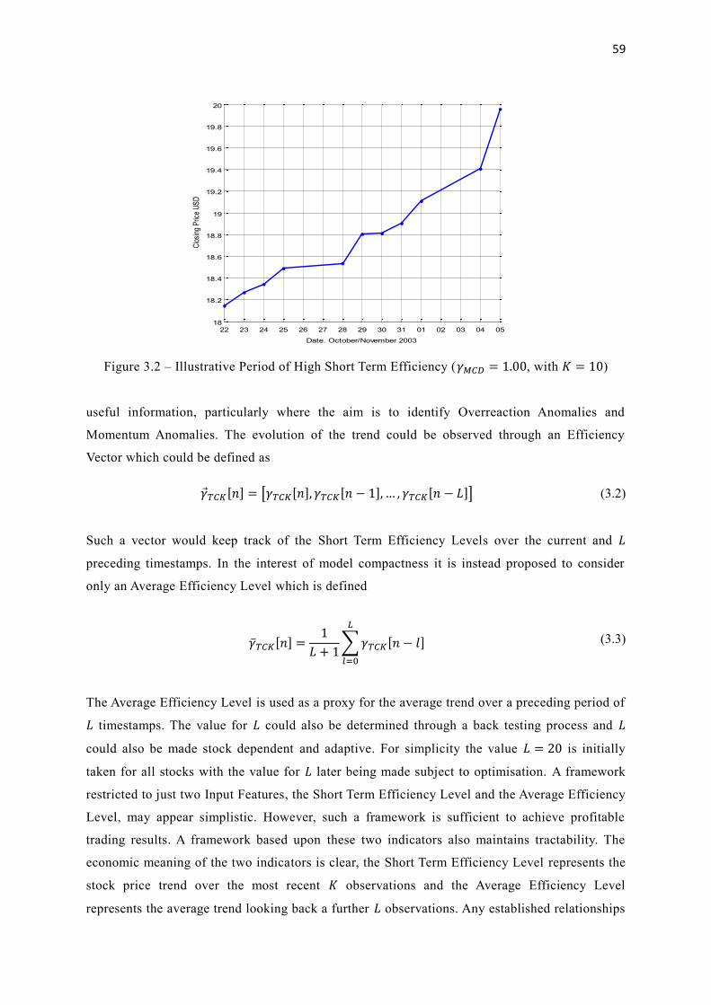
59

Figure 3.2 – Illustrative Period of High Short Term Efficiency (𝛾𝑀𝐶𝐷 = 1.00, with 𝐾 = 10)

useful information, particularly where the aim is to identify Overreaction Anomalies and

Momentum Anomalies. The evolution of the trend could be observed through an Efficiency

Vector which could be defined as

�⃗�𝑇𝐶𝐾[𝑛] = [𝛾𝑇𝐶𝐾[𝑛], 𝛾𝑇𝐶𝐾[𝑛 − 1], … , 𝛾𝑇𝐶𝐾[𝑛 − 𝐿]] (3.2)

Such a vector would keep track of the Short Term Efficiency Levels over the current and 𝐿

preceding timestamps. In the interest of model compactness it is instead proposed to consider

only an Average Efficiency Level which is defined

�̅�𝑇𝐶𝐾[𝑛] =1

𝐿 + 1∑𝛾𝑇𝐶𝐾[𝑛 − 𝑙]

𝐿

𝑙=0

(3.3)

The Average Efficiency Level is used as a proxy for the average trend over a preceding period of

𝐿 timestamps. The value for 𝐿 could also be determined through a back testing process and 𝐿

could also be made stock dependent and adaptive. For simplicity the value 𝐿 = 20 is initially

taken for all stocks with the value for 𝐿 later being made subject to optimisation. A framework

restricted to just two Input Features, the Short Term Efficiency Level and the Average Efficiency

Level, may appear simplistic. However, such a framework is sufficient to achieve profitable

trading results. A framework based upon these two indicators also maintains tractability. The

economic meaning of the two indicators is clear, the Short Term Efficiency Level represents the

stock price trend over the most recent 𝐾 observations and the Average Efficiency Level

represents the average trend looking back a further 𝐿 observations. Any established relationships

22 23 24 25 26 27 28 29 30 31 01 02 03 04 0518

18.2

18.4

18.6

18.8

19

19.2

19.4

19.6

19.8

20

Date. October/November 2003

Clo

sing

Pric

e U

SD

60

between the two indicators would be a relationship between the recent trend and the longer dated

trend of the stock price.

In order to generate a Training Set the Profit and Loss (P&L) of a trade entered to follow the

recent Short Term Trend Direction of a stock can be considered. The Short Term Trend Direction

𝐷𝑇𝐶𝐾[𝑛] observed at timestamp 𝑛 has been defined in Equation (2.10) and is restated below

𝐷𝑇𝐶𝐾[𝑛] = sgn(𝑆𝑇𝐶𝐾[𝑛] − 𝑆𝑇𝐶𝐾[𝑛 − 𝐾]) (3.4)


to zero and takes the value of −1 otherwise. A value of 𝐷𝑇𝐶𝐾[𝑛] = 1 then corresponds to the case

that the stock is seen to be in a recent uptrend and the value of 𝐷𝑇𝐶𝐾[𝑛] = −1 corresponds to the

case that the stock is seen to be in a recent downtrend. The indicator 𝐷𝑇𝐶𝐾[𝑛] provides only

directional information, the Short Term Efficiency Level 𝛾𝑇𝐶𝐾[𝑛] provides a measure of the

strength of the trend. It should be noted that the two indicators 𝐷𝑇𝐶𝐾[𝑛] and 𝛾𝑇𝐶𝐾[𝑛] are defined

over the same interval of 𝐾 observations. A Training Set can be generated such that the 𝑛th

Training Sample is {{𝛾𝑇𝐶𝐾[𝑛], �̅�𝑇𝐶𝐾[𝑛]}, 𝑃𝑇𝐶𝐾[𝑛]}, where 𝛾𝑇𝐶𝐾[𝑛] and �̅�𝑇𝐶𝐾[𝑛] are the Short Term

Efficiency Level and Average Efficiencies Levels as defined above, and 𝑃𝑇𝐶𝐾[𝑛] is the trade

P&L for placing a trade in the same direction as 𝐷𝑇𝐶𝐾[𝑛]. The trade P&L 𝑃𝑇𝐶𝐾[𝑛] is defined as

𝑃𝑇𝐶𝐾[𝑛] = 𝐷𝑇𝐶𝐾[𝑛] ∙(𝑆𝑇𝐶𝐾[𝑗] − 𝑆𝑇𝐶𝐾[𝑛])

𝑆𝑇𝐶𝐾[𝑛] (3.5)

and represents the Holding Period Return from a holding to timestamp 𝑗 > 𝑛 for a trade initiated

at timestamp 𝑛 with direction 𝐷𝑇𝐶𝐾[𝑛]. The determination of the value of 𝑗 is discussed below. It

should be noted that the direction of the trade 𝐷𝑇𝐶𝐾[𝑛] is the direction of the observed stock

price movement over the preceding 𝐾 time intervals and as such the value 𝑃𝑇𝐶𝐾[𝑛] is the P&L of

placing a trade that assumes that the recently realised direction will persist. This is to say that

𝑃𝑇𝐶𝐾[𝑛] is the P&L of placing a trade that assumes a Momentum Based Trading Strategy.

A back testing method could then be used to identify potential historic trading opportunities based on

the averaged realised P&L for trades entered under certain observed conditions of the Short Term

Efficiency Level 𝛾𝑇𝐶𝐾[𝑛] and the Average Efficiency Level �̅�𝑇𝐶𝐾[𝑛]. An illustrative proposed

back testing method is as follows. Values of 𝐾 and 𝐿 are fixed to 10 and 20 respectively. At each

observation 𝑛 a trade is entered into by following the recent direction 𝐷𝑇𝐶𝐾[𝑛], the trade is closed at

the earliest timestamp 𝑗 with (𝑗 > 𝑛) that one or more of the following conditions is found to hold (i)

𝛾𝑇𝐶𝐾[𝑗] < (𝛾𝑇𝐶𝐾[𝑛] − 𝛿𝑇𝐶𝐾[𝑛]) or (ii) �̅�𝑇𝐶𝐾[𝑗] < (�̅�𝑇𝐶𝐾[𝑛] − 𝛿�̅�𝐶𝐾[𝑛]) or (iii) 𝑗 = 𝑛 + 𝐽𝑇𝐶𝐾[𝑛]. The

61

first condition corresponds to the case that the Short Term Efficiency Level has dropped below some

threshold 𝛿𝑇𝐶𝐾[𝑛] of within the Short Term Efficiency Level at the timestamp 𝑛 of trade initiation.

The second condition corresponds to the case that the Average Efficiency Level has dropped below

some threshold 𝛿�̅�𝐶𝐾[𝑛] of within the Average Efficiency Level at the timestamp 𝑛 of trade initiation.

The final condition corresponds to the case that a trade is closed out after 𝐽𝑇𝐶𝐾[𝑛] days if it has not

already been closed out, such a condition is included as a safety catch to break out of trades after

some maximum time. For the purpose of illustrative back testing the following levels are used

𝛿𝑇𝐶𝐾[𝑛] = 0 ∀𝑇𝐶𝐾, 𝑛 and 𝛿�̅�𝐶𝐾[𝑛] = 0 ∀𝑇𝐶𝐾, 𝑛 and 𝐽𝑇𝐶𝐾[𝑛] = 3 ∀𝑇𝐶𝐾, 𝑛. Following back testing,

potential future trading opportunities can then be identified. The trading premise is that stocks can be

separated into the following four broad categories.

Stocks That Show Overreaction Anomalies – For example, for JP Morgan Chase Bank (Bloomberg

Code: JPM EQUITY), a back test from April 2003 to April 2010 reveals that where the Average

Efficiency Level is less than a threshold of 0.50 (�̅�𝐽𝑃𝑀[𝑛] < 0.50), but the Short Term Efficiency

Level is greater than or equal to a threshold of 0.50 (𝛾𝐽𝑃𝑀[𝑛] ≥ 0.50), on average trading profits

could have been made by betting against the direction 𝐷𝐽𝑃𝑀[𝑛]. This is to say that under such

conditions of �̅�𝐽𝑃𝑀[𝑛] and 𝛾𝐽𝑃𝑀[𝑛] a short trade should have been placed when 𝐷𝐽𝑃𝑀[𝑛] = 1 and a

long trade should have been placed otherwise. The combination {�̅�𝐽𝑃𝑀[𝑛] < 0.50, 𝛾𝐽𝑃𝑀[𝑛] ≥ 0.50}

corresponds to the case of a relatively weak average trend as shown by the Average Efficiency Level

with a strong short term trend as shown by the Short Term Efficiency Level. In such a case the short

term trend has typically been seen as transient and would be expected to reverse, this reversal then

represents the existence of a probable Overreaction Anomaly and this is a trading opportunity. In

summary for an overreacting stock like JP Morgan Chase Bank it is seen that Overreaction Anomalies

can be identified under some conditions of the Short Term Efficiency Level and the Average

Efficiency Level, a reversal of the recent short term direction of the stock would then be expected.

Stocks That Show Momentum Anomalies – For example, for United Healthcare (Bloomberg Code:

UNH EQUITY), a back test from April 2003 to April 2010 reveals that where the Average Efficiency

Level is greater than or equal to a threshold of 0.50 (�̅�𝑈𝑁𝐻[𝑛] ≥ 0.50), but the Short Term Efficiency

Level is less than a threshold of 0.75 (𝛾𝑈𝑁𝐻[𝑛] < 0.75), on average trading profits could have been

made by following the direction 𝐷𝑈𝑁𝐻[𝑛]. This is to say that under such conditions of �̅�𝑈𝑁𝐻[𝑛] and

𝛾𝑈𝑁𝐻[𝑛] a long trade should be placed when 𝐷𝑈𝑁𝐻[𝑛] = 1 and a short trade should be placed

otherwise. The conditions {�̅�𝑈𝑁𝐻[𝑛] ≥ 0.50, 𝛾𝑈𝑁𝐻[𝑛] < 0.75} correspond to a large fraction of the

range of possible values of the Short Term Efficiency Level 𝛾𝑈𝑁𝐻[𝑛], and as such it appears that the

value of the Average Efficiency Level �̅�𝑈𝑁𝐻[𝑛] is the dominating factor. Such conditions then seem to

imply that for UNH, if there is a strong Average Efficiency Level then the direction 𝐷𝑈𝑁𝐻[𝑛] would

be expected to sustain and as such the presence of a Momentum Anomaly can be identified.

62

Stocks That Show Both Overreaction and Momentum Anomalies – For other stocks it is possible to

identify a region in the {�̅�𝑇𝐶𝐾[𝑛], 𝛾𝑇𝐶𝐾[𝑛]} plane where a back test would reveal the existence of

Overreaction Anomalies and also to identify a second region where a back test would reveal the

existence of Momentum Anomalies. For example, for Exxon Mobil (Bloomberg Code: XOM

EQUITY), it can be seen from a back test from April 2003 to April 2010 that regions can be isolated

in the {�̅�𝑋𝑂𝑀[𝑛], 𝛾𝑋𝑂𝑀[𝑛]} plane where Overreaction and Momentum Anomalies can be identified.

Not Opportunistic – Other stocks, for example Johnson and Johnson (Bloomberg Code: JNJ

EQUITY) do not reveal any trading opportunities for a back test from April 2003 to April 2010.

The back test results can be summarised by identifying regions in which anomalies arise for trades

which are placed with entry Efficiency Thresholds {𝛾𝑇𝐶𝐾[𝑛], �̅�𝑇𝐶𝐾[𝑛]} above particular levels.

Illustrative results are shown in Figures 3.3 to 3.6, respectively, for the four stocks discussed above JP

Morgan (Bloomberg Code: JPM EQUITY), United Healthcare (Bloomberg Code: UNH EQUITY),

Exxon Mobil (Bloomberg Code: XOM EQUITY) and Johnson and Johnson (Bloomberg Code: JNJ

EQUITY). In each figure regions where on average profits in excess of 30 bps (0.30%) per trade

could have been made by following the direction 𝐷𝑇𝐶𝐾[𝑛] have been highlighted in red and regions

where on average losses in excess of 30 bps per trade could have been made by following the

direction 𝐷𝑇𝐶𝐾[𝑛] have been highlighted in blue. It should be noted that on average profits in excess

of 30 bps could have been made by betting against the direction 𝐷𝑇𝐶𝐾[𝑛] for the regions highlighted

in blue. The blue regions then represent conditions under which Overreaction Anomalies can be

identified and the red regions represent conditions under which Momentum Anomalies can be

identified. The threshold of 30 bps is for the purpose of illustration. In the figures a zero return has

been substituted in any regions where less than 5 trades occurred, this is to remove outlier effects.

Figure 3.3 – Historical Conditions for Anomalies for JPM between April 03 and April 10

Average Efficiency Level

Sho

rt Te

rm E

ffici

ency

Lev

el

0 0.1 0.2 0.3 0.4 0.5 0.6 0.7 0.8 0.9 10

0.1

0.2

0.3

0.4

0.5

0.6

0.7

0.8

0.9

1

63

Figure 3.4 – Historical Conditions for Anomalies for UNH between April 03 and April 10

Figure 3.5 – Historical Conditions for Anomalies for XOM between April 03 and April 10

Figure 3.6 – Historical Conditions for Anomalies for JNJ between April 03 and April 10


Sho

rt Te

rm E

ffici

ency

Lev

el

0 0.1 0.2 0.3 0.4 0.5 0.6 0.7 0.8 0.9 10

0.1

0.2

0.3

0.4

0.5

0.6

0.7

0.8

0.9

1


Sho

rt Te

rm E

ffici

ency

Lev

el

0 0.1 0.2 0.3 0.4 0.5 0.6 0.7 0.8 0.9 10

0.1

0.2

0.3

0.4

0.5

0.6

0.7

0.8

0.9

1


Sho

rt Te

rm E

ffici

ency

Lev

el

0 0.1 0.2 0.3 0.4 0.5 0.6 0.7 0.8 0.9 10

0.1

0.2

0.3

0.4

0.5

0.6

0.7

0.8

0.9

1

64

Having identified historical trading opportunities for each individual stock (as for example in Figures

3.3 to 3.6), it is now possible to define a simple trading strategy at an individual stock level. For each

stock a chart of average trend following P&L for trades entered when the Short Term Efficiency

Level 𝛾𝑇𝐶𝐾[𝑛] and Average Efficiency Level �̅�𝑇𝐶𝐾[𝑛] are above some thresholds could be constructed

(similar to Figures 3.3 to 3.6). Regions where the average trade P&L is above some threshold (30 bps

for example) would be identified as regions where Momentum Anomalies have been identified and as

such in future trend following (Momentum) trades should be placed under the corresponding

conditions. Regions where the average trade P&L is below some level (-0.30% in the examples

above) are identified as regions where Overreaction Anomalies have been identified and as such in

future Reversion Trades should be placed under the corresponding conditions. To illustrate the

profitability of such an approach the case where trade regions are constructed based on back Test Data

from April-2003 to April-2010 is considered. The stock universe is the top 20 constituents (ordered

descending by weight) of the Dow Jones Industrial Average (Ticker INDU INDEX). This stock

universe is chosen as it consists of large market capitalisation stocks that could be easily traded. Such

stocks can also be cheaply borrowed for short selling and sufficiently long closing price histories can

be easily sourced. Having identified potentially profitable trading regions for each stock from a back

test the same regions can then be applied to test for forward generated Profit and Loss (P&L).

The test for P&L considers the time period from April-2010 to April-2013 using trading regions fixed

from the back test using data up to April-2010. For each stock an index is constructed to start at 100

on 09-April-2010. If on a post training trading day 𝑚 a suitable trading opportunity is found, where

suitable is determined according to the generated chart for each stock, then a trade is placed. In each

case the trade is held until the earliest of (i) 𝛾𝑇𝐶𝐾[𝑗] < 𝛾𝑇𝐶𝐾[𝑚] or (ii) �̅�𝑇𝐶𝐾[𝑗] < �̅�𝑇𝐶𝐾[𝑚] or (iii)

𝑗 = 𝑚 + 3. For each trade the invested amount is the current value of the constructed index. If for a

particular stock it is the case that a trade is already active then no other trade will be entered. Table

3.1 presents for each stock the end value of its index over the 3 year testing period. Table 3.1 also

provides information for the total number of days that are spent in live trades for each stock from a

possible 750 business days. The table also provides the number of long and short trades for each

stock. The final row of the table provides the Average Statistics amongst the 20 stocks and it can be

seen that on average only 98 out of 750 possible days are spent in live trade, a proportion of around

only 13%. This is to say that at most times, for any particular stock, the framework does not deem the

environment to be sufficiently conducive for trade entry. This is in keeping with a hypothesis that at

most times stocks should be considered as efficiently priced and hence as such anomalies rarely

occur. The average return over three years per stock is only 4.42% and this may appear to be low, but

it should be viewed against a backdrop of only being in active trade around 13% of the time, higher

returns on investment would be achieved at a Portfolio Level by selecting trading opportunities

amongst those from a wider universe of stocks.

65

Stock Name Ticker Start

Index

End

Index

Trade

Days

Long

Trades

Short

Trades

1 IBM IBM 100.00 107.49 73 36 19

2 Chevron CVX 100.00 99.86 76 14 39

3 3M MMM 100.00 99.99 16 5 9

4 McDonalds MCD 100.00 119.72 97 24 52

5 Untd Tech. UTX 100.00 95.77 100 19 42

6 Exxon XOM 100.00 107.19 15 7 5

7 Boeing BA 100.00 111.89 58 20 29

8 Caterpillar CAT 100.00 96.22 130 37 51

9 Travellers TRV 100.00 103.14 156 25 79

10 J&J JNJ 100.00 100.00 0 0 0

11 P&G PG 100.00 96.15 143 38 60

12 Walmart WMT 100.00 102.43 36 3 19

13 Home Dep. HD 100.00 92.79 198 34 99

14 Am. Exp. AXP 100.00 119.97 311 80 136

15 Untd. Hlth. UNH 100.00 112.00 43 26 6

16 Disney DIS 100.00 107.70 61 18 23

17 Verizon VZ 100.00 97.89 158 32 70

18 Dupont DD 100.00 110.80 26 10 10

19 JP Morgan JPM 100.00 111.82 191 48 81

20 Merck MRK 100.00 95.66 64 10 41

Average 100.00 104.42 97.6 24.3 43.5

Table 3.1- Application of an Introductory Framework to Large Market Capitalisation Stocks

Thus far an introductory framework for identifying Overreaction and Momentum Anomalies has been

presented. The framework is in itself novel and should be recognised as an original contribution to the

field of Technical Analysis. The framework employs the Efficiency Indicator first proposed by

Kaufman [110]. Kaufman proposed the use of a single Short Term Efficiency Indicator for trend

following, his method advocates a trading strategy whereby a direction 𝐷𝑇𝐶𝐾[𝑛] following trade is

placed if the Short Term Efficiency Indicator is high (and so the short term trend is strong) and the

trade is closed when the Short Term Efficiency Indicator begins to weaken. The original Kaufman

approach was geared only towards the use of a single indicator to detect Momentum Anomalies. The

original Kaufman approach does not consider the use of a combination of a Short Term and an

Average Efficiency Level, it also does not consider the detection of Overreaction Anomalies.

The framework that has been presented has a rational economic basis. At the core of the method is the

direct detection of Momentum and Overreaction Anomalies which have been shown to arise through

the behavioural inefficiencies of market participants. As long as such inefficiencies persist the method

would be expected to function. The framework does, however, need to be made adaptive to changing

market conditions as it would not be reasonable to expect the same anomalies to persist over time. To

have an adaptive framework would require the application of Machine Learning techniques.

66

3.3 First Neural Network Approach for Trend Detection

As a first step towards the introduction of Machine Learning techniques the replication of the

approach of the previous sub-section within a Neural Network framework is presented. In the

previous sub-section a Training Set was formed from Training Samples of the form

{{𝛾𝑇𝐶𝐾[𝑛], �̅�𝑇𝐶𝐾[𝑛]}, 𝑃𝑇𝐶𝐾[𝑛]}. The Training Set was used to form regions with threshold values

of 𝛾𝑇𝐶𝐾[𝑛] and �̅�𝑇𝐶𝐾[𝑛] above which the average P&L for a direction 𝐷𝑇𝐶𝐾[𝑛] following trade

was greater than 0.30%, such regions imply the probable detection of Momentum Anomalies. In

addition, regions with threshold values of 𝛾𝑇𝐶𝐾[𝑛] and �̅�𝑇𝐶𝐾[𝑛] above which the average P&L of

a direction following trade was less than -0.30% were also identified, such regions

corresponding to the probable detection of Overreaction Anomalies. The formation of threshold

regions of the Short Term Efficiency Level and the Average Efficiency Level would not provide

data of a form that would be useful for direct decision inference by a Neural Network. Instead it

is proposed that a Training Set consisting of Training Samples of the form

{{𝛾𝑇𝐶𝐾[𝑛], �̅�𝑇𝐶𝐾[𝑛]}, 𝐶𝑇𝐶𝐾[𝑛]} should be used for Neural Network training. Here the Categorised

Trade P&L 𝐶𝑇𝐶𝐾[𝑛] is defined as in Table 3.2. The Categorised Trade P&L 𝐶𝑇𝐶𝐾[𝑛] is based

upon a categorisation threshold 𝜔𝑇𝐶𝐾[𝑛] that can be stock and time dependent.

The categorised trade P&L is based upon the P&L 𝑃𝑇𝐶𝐾[𝑛] for a trade entered at timestamp

𝑛 that follows the Short Term Trend Direction 𝐷𝑇𝐶𝐾[𝑛]. The trade is exited at timestamp 𝑗 > 𝑛

when the earliest of three exit criteria is satisfied (i) 𝛾𝑇𝐶𝐾[𝑗] < (𝛾𝑇𝐶𝐾[𝑛] − 𝛿𝑇𝐶𝐾[𝑛]) or (ii)

�̅�𝑇𝐶𝐾[𝑗] < (�̅�𝑇𝐶𝐾[𝑛] − 𝛿�̅�𝐶𝐾[𝑛]) or (iii) 𝑗 = 𝑛 + 𝐽𝑇𝐶𝐾[𝑛]. The first condition corresponds to the case

that the Short Term Efficiency Level has dropped below some threshold 𝛿𝑇𝐶𝐾[𝑛] of within the Short

Term Efficiency Level at the timestamp 𝑛 of trade initiation. The second condition corresponds to the

case that the Average Efficiency Level has dropped below some threshold 𝛿�̅�𝐶𝐾[𝑛] of within the

Average Efficiency Level at the timestamp 𝑛 of trade initiation. The final condition corresponds to the

case that a trade is closed out after 𝐽𝑇𝐶𝐾[𝑛] days if it has not already been closed out, such a condition

is included as a safety catch to break out of trades after some maximum time.

The categorised trade P&L 𝐶𝑇𝐶𝐾[𝑚] will the eventual trading decision at some post training

timestamp 𝑚 based on the then prevailing Short Term Efficiency Level 𝛾𝑇𝐶𝐾[𝑚] and Average

Category 𝑪𝑻𝑪𝑲[𝒏] Condition

-1 𝑃𝑇𝐶𝐾[𝑛] ≤ −𝜔𝑇𝐶𝐾[𝑛] 0 −𝜔𝑇𝐶𝐾[𝑛] < 𝑃𝑇𝐶𝐾[𝑛] ≤ 𝜔𝑇𝐶𝐾[𝑛] 1 𝑃𝑇𝐶𝐾[𝑛] > 𝜔𝑇𝐶𝐾[𝑛]

Table 3.2 - Proposed Trade Categorisation Scheme for a First Application of a Neural Network

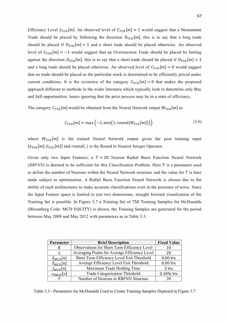
67

Efficiency Level �̅�𝑇𝐶𝐾[𝑚]. An observed level of 𝐶𝑇𝐶𝐾[𝑚] = 1 would suggest that a Momentum

Trade should be placed by following the direction 𝐷𝑇𝐶𝐾[𝑚], this is to say that a long trade

should be placed if 𝐷𝑇𝐶𝐾[𝑚] = 1 and a short trade should be placed otherwise. An observed

level of 𝐶𝑇𝐶𝐾[𝑚] = −1 would suggest that an Overreaction Trade should be placed by betting

against the direction 𝐷𝑇𝐶𝐾[𝑚], this is to say that a short trade should be placed if 𝐷𝑇𝐶𝐾[𝑚] = 1

and a long trade should be placed otherwise. An observed level of 𝐶𝑇𝐶𝐾[𝑚] = 0 would suggest

that no trade should be placed as the particular stock is determined to be efficiently priced under

current conditions. It is the existence of the category 𝐶𝑇𝐶𝐾[𝑚] = 0 that makes the proposed

approach different to methods in the wider literature which typically look to determine only Buy

and Sell opportunities, hence ignoring that the price process may be in a state of efficiency.

The category 𝐶𝑇𝐶𝐾[𝑚] would be obtained from the Neural Network output 𝑊𝑇𝐶𝐾[𝑚] as

𝐶𝑇𝐶𝐾[𝑚] = 𝑚𝑎𝑥 (−1,𝑚𝑖𝑛(1, 𝑟𝑜𝑢𝑛𝑑(𝑊𝑇𝐶𝐾[𝑚]))) (3.6)

where 𝑊𝑇𝐶𝐾[𝑚] is the trained Neural Network output given the post training input

{𝛾𝑇𝐶𝐾[𝑚], �̅�𝑇𝐶𝐾[𝑚]} and 𝑟𝑜𝑢𝑛𝑑(. ) is the Round to Nearest Integer Operator.

Given only two Input Features, a 𝑇 = 20 Neuron Radial Basis Function Neural Network

(RBFNN) is deemed to be sufficient for this Classification Problem. Here 𝑇 is a parameter used

to define the number of Neurons within the Neural Network structure and the value for 𝑇 is later

made subject to optimisation. A Radial Basis Function Neural Network is chosen due to the

ability of such architectures to make accurate classifications even in the presence of noise. Since

the Input Feature space is limited to just two dimensions, straight forward visualization of the

Training Set is possible. In Figure 3.7 a Training Set of 750 Training Samples for McDonalds

(Bloomberg Code: MCD EQUITY) is shown, the Training Samples are generated for the period

between May 2009 and May 2012 with parameters as in Table 3.3.

Parameter Brief Description Fixed Value

𝐾 Observations for Short Term Efficiency Level 10

𝐿 Averaging Points for Average Efficiency Level 20

𝛿𝑀𝐶𝐷[𝑛] Short Term Efficiency Level Exit Threshold 0.00 ∀𝑛

𝛿�̅�𝐶𝐷[𝑛] Average Efficiency Level Exit Threshold 0.00 ∀𝑛

𝐽𝑀𝐶𝐷[𝑛] Maximum Trade Holding Time 3 ∀𝑛

𝜔𝑀𝐶𝐷[𝑛] Trade Categorisation Threshold 0.30% ∀𝑛

𝑇 Number of Neurons in RBFNN Structure 20

Table 3.3 - Parameters for McDonalds Used to Create Training Samples Depicted in Figure 3.7

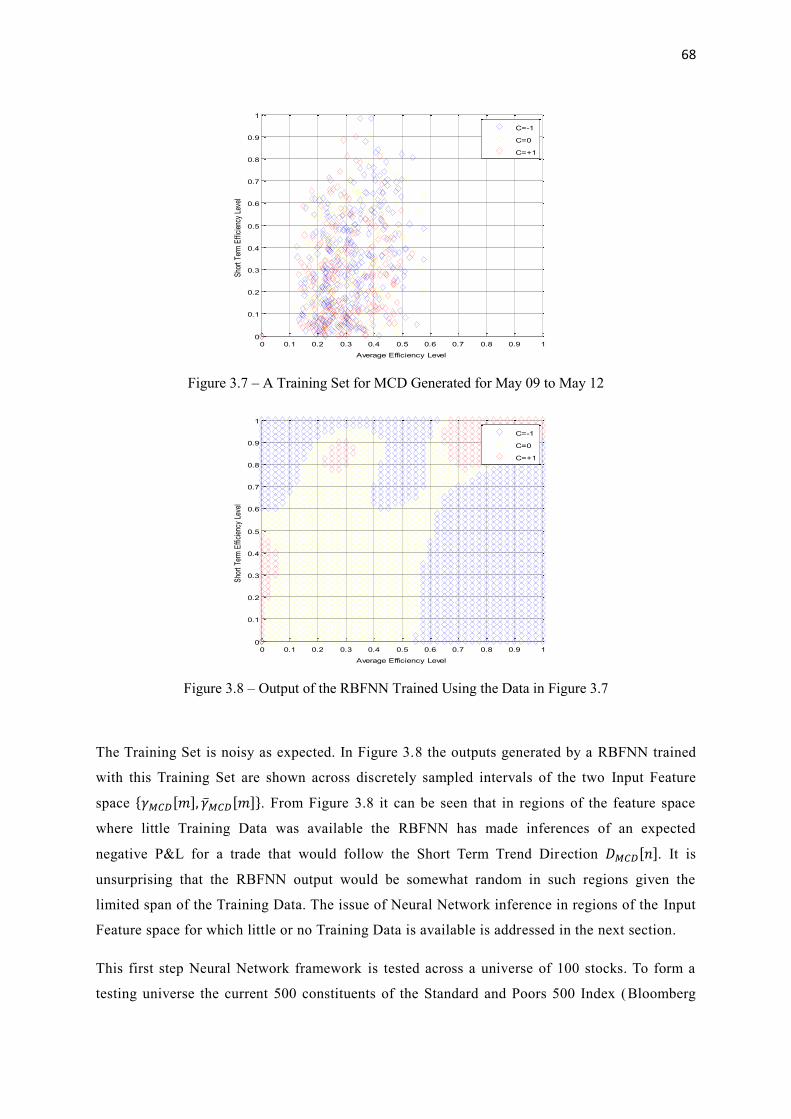
68

Figure 3.7 – A Training Set for MCD Generated for May 09 to May 12

Figure 3.8 – Output of the RBFNN Trained Using the Data in Figure 3.7

The Training Set is noisy as expected. In Figure 3.8 the outputs generated by a RBFNN trained

with this Training Set are shown across discretely sampled intervals of the two Input Feature

space {𝛾𝑀𝐶𝐷[𝑚], �̅�𝑀𝐶𝐷[𝑚]}. From Figure 3.8 it can be seen that in regions of the feature space

where little Training Data was available the RBFNN has made inferences of an expected

negative P&L for a trade that would follow the Short Term Trend Direction 𝐷𝑀𝐶𝐷[𝑛]. It is

unsurprising that the RBFNN output would be somewhat random in such regions given the

limited span of the Training Data. The issue of Neural Network inference in regions of the Input

Feature space for which little or no Training Data is available is addressed in the next section.

This first step Neural Network framework is tested across a universe of 100 stocks. To form a

testing universe the current 500 constituents of the Standard and Poors 500 Index (Bloomberg

0 0.1 0.2 0.3 0.4 0.5 0.6 0.7 0.8 0.9 10

0.1

0.2

0.3

0.4

0.5

0.6

0.7

0.8

0.9

1


Sho

rt Te

rm E

ffici

ency

Lev

el

C=-1

C=0

C=+1

0 0.1 0.2 0.3 0.4 0.5 0.6 0.7 0.8 0.9 10

0.1

0.2

0.3

0.4

0.5

0.6

0.7

0.8

0.9

1


Sho

rt Te

rm E

ffici

ency

Lev

el

C=-1

C=0

C=+1

69

Code: SPX INDEX) are taken and ordered by descending market capitalisation. Any stocks for

which 10 years of daily closing price information is not available are removed. For example

Google (Bloomberg Code: GOOG EQUITY) which was listed on 19th

August 2004 is removed

from consideration. The remaining universe consists of 447 stocks. To form an initial sub-

universe a stratified sample of the 447 stocks is formed by selecting every 4th

stock, such that

the 4th

, 8th

, .. , 400th

largest stocks are taken. A stratified sample is taken to give a sub-universe

that encompasses a large range of stocks with different market capitalisations, using a stratified

cross section would eliminate any potential sample selection bias that may occur for example if

the top or bottom 100 stocks are selected. For reference the first stock in the universe of 447

stocks is Apple (Bloomberg Code: AAPL EQUITY) with a market capitalisation, as at 03 June

2013, of 423 Billion USD and the last is Advanced Micro Devices (Bloomberg Code: AMD

EQUITY) with a market capitalisation of under 3 Billion USD. This initial 447 stock universe,

and any sub-universes, then represent groups of liquid stocks that can be easily traded. Market

data for these stocks can be easily sourced. The isolation of 100 stocks creates in sample and out

of sample data. Such a partition allows strategy development to be carried out on the in sample

data and final testing on the remaining out of sample data.

In addition, in order to eliminate any potential time period bias issues it is important to evaluate

performance across a wide time span that would encompass a range of market conditions.

General consensus amongst Financial Engineers is that a method should be tested across a time

period that is sufficiently long to encompass at least one bull market, one bear market and some

significant periods of sideways movement. For testing of this first Neural Network structure a

period of around 10 years spanning from May 2003 to April 2013 is considered. Such a time

period encompasses a wide range of market conditions including the 2008 Global Financial

Crisis [111], for reference the VIX ‘Investor Fear Gauge’ [112] over the test period was in the

range from 10.4 to 59.9, illustrating a wide market volatility range. Closing price data has been

sourced from Bloomberg and has been back adjusted for stock splits and dividends.

For each stock the Neural Network is retrained every 𝑀 = 250 business days (a period of around

1 calendar year) using data for the preceding 𝑁 = 750 business days (a period of around 3

calendar years). Such a division of the available data would give 7 non-overlapping sets of test

results. The variables 𝑀 and 𝑁 are used, respectively, to define the number of timestamps before

retraining and the number of Training Samples within a Training Set, these will later be made

subject to optimisation. Test results are summarized in Table 3.4. A brief description of the

contents of the rows of Table 3.4 is as given below.

Num. Trades – Is the Total Number of Trades generated across the 100 stocks divided by 100.

This then gives the average number of trades generated for each stock within each Test Set.

70

Measure Test Set 1 Test Set 2 Test Set 3 Test Set 4 Test Set 5 Test Set 6 Test Set 7

Training Start 29/05/03 25/05/04 23/05/05 19/05/06 18/05/07 15/05/08 13/05/09

Training End 19/05/06 18/05/07 15/05/08 13/05/09 11/05/10 06/05/11 03/05/12

Testing Start 22/05/06 21/05/07 16/05/08 14/05/09 12/05/10 09/05/11 04/05/12

Testing End 21/05/07 16/05/08 14/05/09 12/05/10 09/05/11 04/05/12 06/05/13

Num. Trades 9.0 6.4 5.6 13.1 10.4 7.1 13.1 % Profitable 50.6% 51.6% 53.8% 51.9% 55.0% 55.7% 52.5% Total P&L 0.6% -0.8% 4.5% 0.1% 1.6% 1.9% 0.1%

P&L Per Trade 0.06% -0.10% 0.64% 0.01% 0.14% 0.24% 0.01% Trade Days 15.3 11.8 10.4 20.3 16.0 11.3 21.2

Average Days 1.5 1.5 1.5 1.4 1.4 1.4 1.4

Table 3.4 - Average Performance Figures for a First Application of a Neural Network

% Profitable – Is the Total Number of Profitable Trades generated across the 100 stocks divided

by the Total Number of Trades generated across the 100 stocks. This then gives the proportion of

profitable trades across all stocks considered together.

Total P&L – Is the Total P&L generated by all the trades across the 100 stocks divided by the

number of stocks for which a non-zero number of trades occurred. This is then the Average Total

P&L per stock for those stocks for which some trades had occurred.

P&L Per Trade - Is the Total P&L generated by all the trades across the 100 stocks divided by

the Total Number of Trades generated across the 100 stocks. This is then the Average P&L per

trade across all stocks considered together.

Trade Days – Is the Total Days spent in trade by all the trades across the 100 stocks divided by

the number of stocks for which a non-zero number of trades occurred. This is then the Average

Number of Days spent in trades for each stock for which some trades had occurred.

Average Days – Is the Total Days spent in trade by all the trades across the 100 stocks divided

by the Total Number of Trades generated across the 100 stocks. This is then the Average duration

per trade across all stocks considered together.

From Table 3.4 it can be seen that on average there are under 65 trades placed per single stock

from a possible 1750 trades per name over the 7 year test period. The average trade duration is

around 1.5 days and therefore on average, for each single stock, there is no investment being

made around 95% of the time. This illustrates a difference between the proposed framework and

many of the methods presented in the literature which look to predict the next day direction and

to follow that. The presented framework looks only to trade when conditions are deemed

suitable and as such very few trading opportunities are identified per single stock. At this stage a

foundation has been established, in the next section a number of improvements are developed.

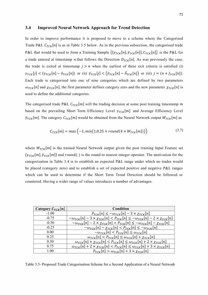
71

3.4 Improved Neural Network Approach for Trend Detection

In order to improve performance it is proposed to move to a scheme where the Categorised

Trade P&L 𝐶𝑇𝐶𝐾[𝑛] is as in Table 3.5 below. As in the previous subsection, the categorised trade

P&L that would be used to form a Training Sample {{𝛾𝑇𝐶𝐾[𝑛], �̅�𝑇𝐶𝐾[𝑛]}, 𝐶𝑇𝐶𝐾[𝑛]} is the P&L for

a trade entered at timestamp 𝑛 that follows the Direction 𝐷𝑇𝐶𝐾[𝑛]. As was previously the case,

the trade is exited at timestamp 𝑗 > 𝑛 when the earliest of three exit criteria is satisfied (i)

𝛾𝑇𝐶𝐾[𝑗] < (𝛾𝑇𝐶𝐾[𝑛] − 𝛿𝑇𝐶𝐾[𝑛]) or (ii) �̅�𝑇𝐶𝐾[𝑗] < (�̅�𝑇𝐶𝐾[𝑛] − 𝛿�̅�𝐶𝐾[𝑛]) or (iii) 𝑗 = (𝑛 + 𝐽𝑇𝐶𝐾[𝑛]).

Each trade is categorised into one of nine categories which are defined by two parameters

𝜔𝑇𝐶𝐾[𝑛] and 𝜒𝑇𝐶𝐾[𝑛], the first parameter defines category zero and the new parameter 𝜒𝑇𝐶𝐾[𝑛] is

used to define the additional categories.

The categorised trade P&L 𝐶𝑇𝐶𝐾[𝑚] will the trading decision at some post training timestamp 𝑚

based on the prevailing Short Term Efficiency Level 𝛾𝑇𝐶𝐾[𝑚] and Average Efficiency Level

�̅�𝑇𝐶𝐾[𝑚]. The category 𝐶𝑇𝐶𝐾[𝑚] would be obtained from the Neural Network output 𝑊𝑇𝐶𝐾[𝑚] as

𝐶𝑇𝐶𝐾[𝑚] = 𝑚𝑎𝑥 (−1,𝑚𝑖𝑛(1,0.25 × 𝑟𝑜𝑢𝑛𝑑(4 ×𝑊𝑇𝐶𝐾[𝑚]))) (3.7)

where 𝑊𝑇𝐶𝐾[𝑚] is the trained Neural Network output given the post training Input Feature set

{𝛾𝑇𝐶𝐾[𝑚], �̅�𝑇𝐶𝐾[𝑚]} and 𝑟𝑜𝑢𝑛𝑑(. ) is the round to nearest integer operator. The motivation for the

categorization in Table 3.4 is to establish an expected P&L range under which no trades would

be placed (category zero) and to establish a set of expected positive and negative P&L ranges

which can be used to determine if the Short Term Trend Direction should be followed or

countered. Having a wider range of values introduces a number of advantages.

Category 𝑪𝑻𝑪𝑲[𝒏] Condition

-1.00 𝑃𝑇𝐶𝐾[𝑛] ≤ −𝜔𝑇𝐶𝐾[𝑛] − 3 × 𝜒𝑇𝐶𝐾[𝑛] -0.75 −𝜔𝑇𝐶𝐾[𝑛] − 3 × 𝜒𝑇𝐶𝐾[𝑛] < 𝑃𝑇𝐶𝐾[𝑛] ≤ −𝜔𝑇𝐶𝐾[𝑛] − 2 × 𝜒𝑇𝐶𝐾[𝑛] -0.50 −𝜔𝑇𝐶𝐾[𝑛] − 2 × 𝜒𝑇𝐶𝐾[𝑛] < 𝑃𝑇𝐶𝐾[𝑛] ≤ −𝜔𝑇𝐶𝐾[𝑛] − 𝜒𝑇𝐶𝐾[𝑛] -0.25 −𝜔𝑇𝐶𝐾[𝑛] − 𝜒𝑇𝐶𝐾[𝑛] < 𝑃𝑇𝐶𝐾[𝑛] ≤ −𝜔𝑇𝐶𝐾[𝑛] 0.00 −𝜔𝑇𝐶𝐾[𝑛] < 𝑃𝑇𝐶𝐾[𝑛] ≤ 𝜔𝑇𝐶𝐾[𝑛] 0.25 𝜔𝑇𝐶𝐾[𝑛] < 𝑃𝑇𝐶𝐾[𝑛] ≤ 𝜔𝑇𝐶𝐾[𝑛] + 𝜒𝑇𝐶𝐾[𝑛] 0.50 𝜔𝑇𝐶𝐾[𝑛] + 𝜒𝑇𝐶𝐾[𝑛] < 𝑃𝑇𝐶𝐾[𝑛] ≤ 𝜔𝑇𝐶𝐾[𝑛] + 2 × 𝜒𝑇𝐶𝐾[𝑛] 0.75 𝜔𝑇𝐶𝐾[𝑛] + 2 × 𝜒𝑇𝐶𝐾[𝑛] < 𝑃𝑇𝐶𝐾[𝑛] ≤ 𝜔𝑇𝐶𝐾[𝑛] + 3 × 𝜒𝑇𝐶𝐾[𝑛] 1.00 𝑃𝑇𝐶𝐾[𝑛] > 𝜔𝑇𝐶𝐾[𝑛] + 3 × 𝜒𝑇𝐶𝐾[𝑛]

Table 3.5- Proposed Trade Categorisation Scheme for a Second Application of a Neural Network

72

The first and most significant advantage of an extended categorisation is that the terminal

categories of {−1} and {1} can now be used to categorise outliers or price shocks in the Training

Set. Such price shocks correspond to unusually large positive or negative P&L that had occurred

for a handful of Training Samples in the Training Set. The treatment of price shocks is an

important practical consideration that is typically overlooked in the development of trading strategies.

A trading strategy that has been somehow optimally fitted over Training Data because of the presence

of price shocks should not be expected to later perform well in reality. Price shocks are unpredictable

and fitting to such shocks may be considered a form of overfitting. It should be noted that the

approach taken here has not removed price shocks from the data but has rather categorised them

correctly as shocks, the difference may appear subtle but it is important. The complete removal of

price shocks from data could be dangerous, an example is that of Long Term Capital Management

(LTCM) who had developed trading strategies with the removal of price shocks [113], their basis for

removal was that they deemed such shocks to be unrealistic. The eventual collapse of LTCM caused

losses that exceeded 4 Billion USD. Again it should be highlighted that the classification process

taken herein has not removed price shocks but has categorised them as outliers. The second advantage

of an extended classification is that it allows for the more intelligent allocation of assets at a Portfolio

level. Given a fixed pool of investment cash, such a categorisation could allow the later selection of

potential opportunities that have the highest expected P&L.

The development thus far has focussed on the use of a Radial Basis Function Neural Network

(RBFNN) as a classification tool. However such a Neural Network structure could also be used as a

prediction tool. For example the RBFNN could be used to predict the expected stock price at some

point in the future. However if such a prediction type approach were taken, there would still need to

be some post prediction classification to create a no-trade (zero) category and to create categories for

outliers. It has therefore been decided to take a classification approach as the creation of zero trade

and outlier categories can then be integrated directly into the Neural Network structure.

In Figure 3.9 a Training Set of 750 Training Samples for McDonalds (Bloomberg Code: MCD

EQUITY) is shown, the Training Samples are again generated on the daily closes between May

2009 and May 2012 with parameter values fixed as in Table 3.6. In Figure 3.10 the outputs

generated by a 𝑇 = 20 Neuron RBFNN trained with this data are shown across discretely

sampled intervals of the range of possible values of the two Input Feature Space

{𝛾𝑀𝐶𝐷[𝑚], �̅�𝑀𝐶𝐷[𝑚]}. Again the issue of random inferences in regions where little or no Training

Data was available can be seen. It may be argued that this issue can be ignored. If a large

Training Set is devoid of Training Samples that fall in some region of feature space, it may then

be expected, in practice, to confront such regions of feature space with a low probability and

therefore the Neural Network inferences may not be statistically considered so important.

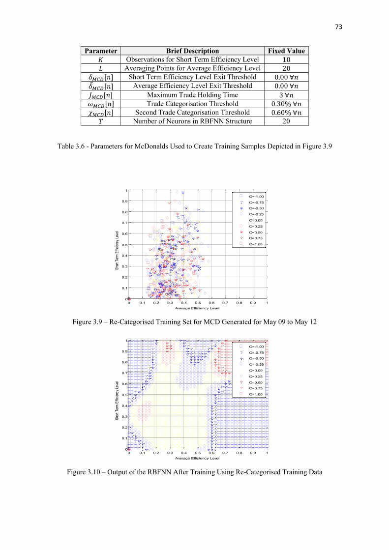
73

Parameter Brief Description Fixed Value

𝐾 Observations for Short Term Efficiency Level 10

𝐿 Averaging Points for Average Efficiency Level 20

𝛿𝑀𝐶𝐷[𝑛] Short Term Efficiency Level Exit Threshold 0.00 ∀𝑛

𝛿�̅�𝐶𝐷[𝑛] Average Efficiency Level Exit Threshold 0.00 ∀𝑛

𝐽𝑀𝐶𝐷[𝑛] Maximum Trade Holding Time 3 ∀𝑛

𝜔𝑀𝐶𝐷[𝑛] Trade Categorisation Threshold 0.30% ∀𝑛

𝜒𝑀𝐶𝐷[𝑛] Second Trade Categorisation Threshold 0.60% ∀𝑛 𝑇 Number of Neurons in RBFNN Structure 20

Table 3.6 - Parameters for McDonalds Used to Create Training Samples Depicted in Figure 3.9

Figure 3.9 – Re-Categorised Training Set for MCD Generated for May 09 to May 12

Figure 3.10 – Output of the RBFNN After Training Using Re-Categorised Training Data

0 0.1 0.2 0.3 0.4 0.5 0.6 0.7 0.8 0.9 10

0.1

0.2

0.3

0.4

0.5

0.6

0.7

0.8

0.9

1


Sho

rt Te

rm E

ffici

ency

Lev

el

C=-1.00

C=-0.75

C=-0.50

C=-0.25

C=0.00

C=0.25

C=0.50

C=0.75

C=1.00

0 0.1 0.2 0.3 0.4 0.5 0.6 0.7 0.8 0.9 10

0.1

0.2

0.3

0.4

0.5

0.6

0.7

0.8

0.9

1


Sho

rt Te

rm E

ffici

ency

Lev

el

C=-1.00

C=-0.75

C=-0.50

C=-0.25

C=0.00

C=0.25

C=0.50

C=0.75

C=1.00

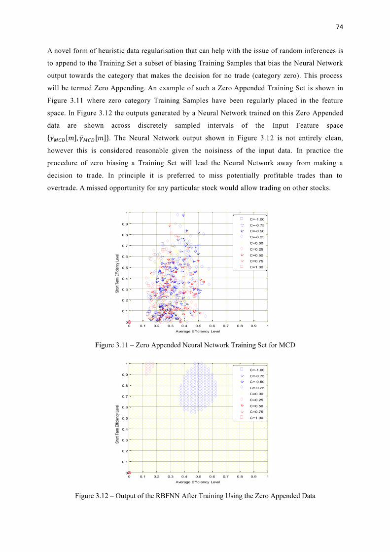
74

A novel form of heuristic data regularisation that can help with the issue of random inferences is

to append to the Training Set a subset of biasing Training Samples that bias the Neural Network

output towards the category that makes the decision for no trade (category zero). This process

will be termed Zero Appending. An example of such a Zero Appended Training Set is shown in

Figure 3.11 where zero category Training Samples have been regularly placed in the feature

space. In Figure 3.12 the outputs generated by a Neural Network trained on this Zero Appended

data are shown across discretely sampled intervals of the Input Feature space

{𝛾𝑀𝐶𝐷[𝑚], �̅�𝑀𝐶𝐷[𝑚]}. The Neural Network output shown in Figure 3.12 is not entirely clean,

however this is considered reasonable given the noisiness of the input data. In practice the

procedure of zero biasing a Training Set will lead the Neural Network away from making a

decision to trade. In principle it is preferred to miss potentially profitable trades than to

overtrade. A missed opportunity for any particular stock would allow trading on other stocks.

Figure 3.11 – Zero Appended Neural Network Training Set for MCD

Figure 3.12 – Output of the RBFNN After Training Using the Zero Appended Data

0 0.1 0.2 0.3 0.4 0.5 0.6 0.7 0.8 0.9 10

0.1

0.2

0.3

0.4

0.5

0.6

0.7

0.8

0.9

1


Sho

rt Te

rm E

ffici

ency

Lev

el

C=-1.00

C=-0.75

C=-0.50

C=-0.25

C=0.00

C=0.25

C=0.50

C=0.75

C=1.00

0 0.1 0.2 0.3 0.4 0.5 0.6 0.7 0.8 0.9 10

0.1

0.2

0.3

0.4

0.5

0.6

0.7

0.8

0.9

1


Sho

rt Te

rm E

ffici

ency

Lev

el

C=-1.00

C=-0.75

C=-0.50

C=-0.25

C=0.00

C=0.25

C=0.50

C=0.75

C=1.00

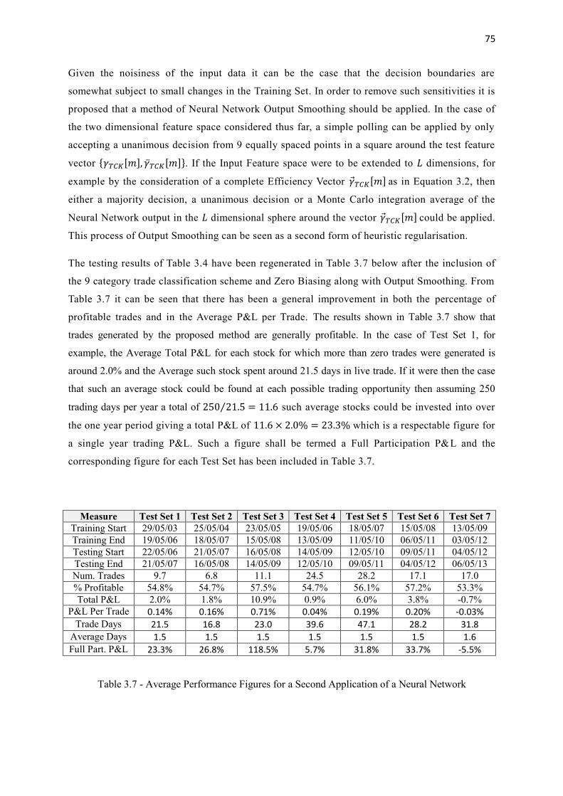
75

Given the noisiness of the input data it can be the case that the decision boundaries are

somewhat subject to small changes in the Training Set. In order to remove such sensitivities it is

proposed that a method of Neural Network Output Smoothing should be applied. In the case of

the two dimensional feature space considered thus far, a simple polling can be applied by only

accepting a unanimous decision from 9 equally spaced points in a square around the test feature

vector {𝛾𝑇𝐶𝐾[𝑚], �̅�𝑇𝐶𝐾[𝑚]}. If the Input Feature space were to be extended to 𝐿 dimensions, for

example by the consideration of a complete Efficiency Vector �⃗�𝑇𝐶𝐾[𝑚] as in Equation 3.2, then

either a majority decision, a unanimous decision or a Monte Carlo integration average of the

Neural Network output in the 𝐿 dimensional sphere around the vector �⃗�𝑇𝐶𝐾[𝑚] could be applied.

This process of Output Smoothing can be seen as a second form of heuristic regularisation.

The testing results of Table 3.4 have been regenerated in Table 3.7 below after the inclusion of

the 9 category trade classification scheme and Zero Biasing along with Output Smoothing. From

Table 3.7 it can be seen that there has been a general improvement in both the percentage of

profitable trades and in the Average P&L per Trade. The results shown in Table 3.7 show that

trades generated by the proposed method are generally profitable. In the case of Test Set 1, for

example, the Average Total P&L for each stock for which more than zero trades were generated is

around 2.0% and the Average such stock spent around 21.5 days in live trade. If it were then the case

that such an average stock could be found at each possible trading opportunity then assuming 250

trading days per year a total of 250 21.5⁄ = 11.6 such average stocks could be invested into over

the one year period giving a total P&L of 11.6 × 2.0% = 23.3% which is a respectable figure for

a single year trading P&L. Such a figure shall be termed a Full Participation P&L and the

corresponding figure for each Test Set has been included in Table 3.7.

Measure Test Set 1 Test Set 2 Test Set 3 Test Set 4 Test Set 5 Test Set 6 Test Set 7

Training Start 29/05/03 25/05/04 23/05/05 19/05/06 18/05/07 15/05/08 13/05/09

Training End 19/05/06 18/05/07 15/05/08 13/05/09 11/05/10 06/05/11 03/05/12

Testing Start 22/05/06 21/05/07 16/05/08 14/05/09 12/05/10 09/05/11 04/05/12

Testing End 21/05/07 16/05/08 14/05/09 12/05/10 09/05/11 04/05/12 06/05/13

Num. Trades 9.7 6.8 11.1 24.5 28.2 17.1 17.0

% Profitable 54.8% 54.7% 57.5% 54.7% 56.1% 57.2% 53.3%

Total P&L 2.0% 1.8% 10.9% 0.9% 6.0% 3.8% -0.7%

P&L Per Trade 0.14% 0.16% 0.71% 0.04% 0.19% 0.20% -0.03% Trade Days 21.5 16.8 23.0 39.6 47.1 28.2 31.8

Average Days 1.5 1.5 1.5 1.5 1.5 1.5 1.6 Full Part. P&L 23.3% 26.8% 118.5% 5.7% 31.8% 33.7% -5.5%

Table 3.7 - Average Performance Figures for a Second Application of a Neural Network

76

3.5 Optimising Neural Network Trend Detection

The approach thus far has established a Neural Network framework that has been shown to be

profitable on average across a universe of 100 stocks and over an extensive time period that spans 7

years and includes a wide range of market conditions. A number of parameters within the framework

have been selected manually and these parameters could be optimised to improve system

performance. A summary of the parameters that are open to optimisation is given in Table 3.8 below.

From Table 3.8 it can be seen that some of the parameters have been kept fixed whilst the range for

optimisation has been defined for other parameters. The value of the Number of Observations for the

Short Term Efficiency Level will be fixed at 10 (𝐾 = 𝐾𝑇𝐶𝐾[𝑛] = 10∀𝑇𝐶𝐾, 𝑛) as the value of 𝐾 will

be used to define the strategy. This is to say that the optimisation of a strategy of type 𝐾𝑇𝐶𝐾[𝑛] =

10∀ 𝑇𝐶𝐾, 𝑛 is considered. The number of samples between retraining has also been fixed to 250

days (𝑀𝑇𝐶𝐾[𝑛] = 250 ∀𝑇𝐶𝐾, 𝑛), in practice the time between retraining would be dependent

upon the availability of computational resources and upon changes in market conditions. A fixed

value of 𝑀𝑇𝐶𝐾[𝑛] = 250 ∀𝑇𝐶𝐾, 𝑛 however allows the available data to be broken into sets of

sequential one year Test Data and this allows a straightforward representation of testing results.

All other parameters are open to optimisation and the possible ranges are as specified in Table

3.8, the use of optimisation bounds will aid the convergence of any optimisation technique.

In optimising parameters a measure of system performance must be chosen. In the wider literature the

common measure of system performance that is employed is the percentage accuracy of the prediction

of next day stock price direction (% Profitable in Table 3.7). However, it is not uncommon for

successful technical expert traders to employ a model that has a directional prediction accuracy of less

than 50%. Directional prediction is not in itself useful, the purpose of trading is to generate profits and

a more useful measure to optimise may be either the P&L per Trade or the P&L per Stock.

Parameter Comment

𝐾𝑇𝐶𝐾[𝑛] Observations for Short Term Efficiency Level. Will keep fixed at 10 to define strategy

𝐿𝑇𝐶𝐾[𝑛] Averaging Points for Average Efficiency Level. Can be optimized in range [5,50]

𝛿𝑇𝐶𝐾[𝑛] Short Term Efficiency Level Exit Threshold. Can be optimized in range [0,0.30]

𝛿�̅�𝐶𝐾[𝑛] Average Efficiency Level Exit Threshold. Can be optimized in range [0,0.30]

𝐽𝑇𝐶𝐾[𝑛] Maximum Trade Holding Time Days. Can be optimized in range [1,10]

𝜔𝑇𝐶𝐾[𝑛] Trade Categorisation Threshold. Can be optimized in range [0.10%,1.00%]

𝜒𝑇𝐶𝐾[𝑛] Second Trade Categorisation Threshold. Can be optimized in range [0.10%,2.00%]

𝑇𝑇𝐶𝐾[𝑛] Number of Neurons in RBFNN Structure. Can be optimized in the range [4,40]

𝑁𝑇𝐶𝐾[𝑛] Length of Training Window. Can be optimized in the range [50,1000]

𝑀𝑇𝐶𝐾[𝑛] Samples between retraining. Will keep fixed at 250 for annual retraining

Table 3.8 - Summary of Parameters that are Open to Optimisation

77

Optimisation to maximise P&L however may lead to a combination of system parameters that is

geared towards high risk trading and this would be undesirable. Profitability should always be seen in

a risk context and therefore it is instead proposed that the P&L to Risk ratio should be optimised. A

P&L to Risk measure that can be defined is the Annualised Information Ratio over a period (𝑚1,𝑚2]

Ι𝑇𝐶𝐾(𝑚1,𝑚2] =P𝑇𝐶𝐾(𝑚1,𝑚2] × 250/ND𝑇𝐶𝐾(𝑚1,𝑚2]

√(SD𝑇𝐶𝐾(𝑚1,𝑚2])2 × 250/ND𝑇𝐶𝐾(𝑚1,𝑚2]

(3.8)

where P𝑇𝐶𝐾(𝑚1,𝑚2] is the Total Percentage P&L for all trades generated on the stock with

Ticker 𝑇𝐶𝐾 over the time period (𝑚1,𝑚2], SD𝑇𝐶𝐾(𝑚1,𝑚2] is the standard deviation of the

Percentage P&L for trades over the same time period and ND𝑇𝐶𝐾(𝑚1,𝑚2] is the Total Number of

Days spent in active trade over the time period (𝑚1, 𝑚2]. The factor 250/ND𝑇𝐶𝐾(𝑚1,𝑚2] is

applied as an Annualisation Factor under the assumption of 250 trading days per annum. It

should be noted that the Annualisation Factor adjustment is applied to the Square of the Standard

Deviation of the P&L (the variance) under the assumption of additive variances with the

assumption of a zero covariance between the P&L of successive trades for stock 𝑇𝐶𝐾. The

application of an Annualisation Factor to give an Annualised Information Ratio would allow a like

for like comparison of performance for trading strategies that consider time periods of different

duration. The numerator of Ι𝑇𝐶𝐾(𝑚1,𝑚2] can be seen as akin to the Annual Full Participation

P&L and the denominator of Ι𝑇𝐶𝐾(𝑚1,𝑚2] can be seen as equivalent to an Annual Full

Participation Volatility.

The measure Ι𝑇𝐶𝐾(𝑚1,𝑚2] may be adjusted to include Transaction Costs, a real world effect that

is largely ignored in the academic literature and that has not been considered thus far. The

Annual Full Participation Volatility may also be floored to prevent Ι𝑇𝐶𝐾(𝑚1,𝑚2] from blowing

up under low volatility conditions; a suitable level for such a floor would be 3%. In addition the

Annualisation Factor may be capped to prevent an optimisation that finds just a few profitable

trades and as such this would help to prevent an optimisation that is based on just outliers. A

suitable Annulisation Factor Cap would be 10 and this would be equivalent to an optimisation

based on an assumption that a particular stock would spend at least 25 days in active trade. The

Modified Annualised Information Ratio can then be defined as

Ι̇𝑇𝐶𝐾(𝑚1,𝑚2] =(P𝑇𝐶𝐾(𝑚1,𝑚2] − 𝑡𝑇𝐶𝐾 × NT𝑇𝐶𝐾(𝑚1,𝑚2]) × min (10,250/ND𝑇𝐶𝐾(𝑚1,𝑚2])

𝑚𝑎𝑥(0.03,√(SD𝑇𝐶𝐾(𝑚1,𝑚2])2 ×min (10,250/ND𝑇𝐶𝐾(𝑚1,𝑚2]))

(3.9)

where NT𝑇𝐶𝐾(𝑚1,𝑚2] is the Number of Trades generated for stock 𝑇𝐶𝐾 over the time period

(𝑚1,𝑚2] and 𝑡𝑇𝐶𝐾 is the Transaction Cost per Trade for trades generated on stock 𝑇𝐶𝐾. It should

78

be noted that the format of the Transaction Cost per Trade is as a percentage of the Stock Price

at the time of trade initiation and as such is akin to the type of Transaction Cost that would be

faced by an institutional investor.

Standard off the shelf optimisation tools often aim to minimise rather than maximise a Cost

Function and as such it is instead proposed to minimise the following Cost Function

Ψ𝑇𝐶𝐾(𝑚1, 𝑚2] = 𝑙𝑛 (1

max (0.1, Ι̇𝑇𝐶𝐾(𝑚1, 𝑚2])) (3.10)

where 𝑙𝑛(. ) is the Natural Logarithm Operator. The presence of the floor of 0.1 applied to the Modified

Annualised Information Ratio has the effect of giving a value of 𝑙𝑛(10) ≈ 2.30 for the Cost Function

Ψ𝑇𝐶𝐾(𝑚1,𝑚2] in the case that Ι̇𝑇𝐶𝐾(𝑚1,𝑚2] takes on either a negative or very small positive

value. The mapping from the Modified Annualised Information Ratio Ι̇𝑇𝐶𝐾(𝑚1,𝑚2] to the

proposed Cost Function Ψ𝑇𝐶𝐾(𝑚1,𝑚2] can be viewed in Figure 3.13 below. From Figure 3.13

the effect of the floor of 0.1 can be seen in that any negative values for the Modified Annualised

Information Ratio have been mapped to a fixed positive value. The role of the Natural Logarithm

Operator is to prevent the suppression of negative troughs that occur at high positive levels of

the Modified Annualised Information Ratio. The purpose of these two modifications to the Cost

Function is to help to provide a cleaner global minimum for an optimisation algorithm to locate.

At this stage a Cost Function of a form that is suitable for optimisation has been established.

Optimisation may be considered on a stock by stock basis such that a set of parameters o f the

types shown in Table 3.7 could be found for each individual stock. However financial data is

Figure 3.13 – Mapping to Proposed Cost Function

79

inherently noisy and a direct global parameter optimization for an individual stock would find a

global minimum to the proposed Cost Function that is heavily affected by noise. A method to

deal with this noise is to exploit The Law of Large Numbers and attempt to average away noise

and instead find initially the parameters that minimise the average of the proposed Cost Function

across a larger Portfolio of stocks. Simulated Annealing can be applied as a global parameter

optimisation technique. The universe of stocks considered for optimisation is the same 100

stocks that have been used to generate the results in Table 3.7. It is proposed that Test Set 2 is

used as an Optimisation Data Set, this is to say that values for the parameters in Table 3.8 should

be optimised to give a global minimum in the average of the proposed Cost Function over Test

Set 2 (21/05/07 to 16/05/08). Test Set 2 is chosen rather than Test Set 1 to provide an additional

set of possible training points for the optimisation of the Length of the Training Window. The

optimised values for the variable parameters are then as shown in Table 3.9 below under the

assumption of a Transaction Cost Level of 𝑡𝑇𝐶𝐾[𝑚] = 0.04% ∀ 𝑇𝐶𝐾,𝑚

Having established parameter values that are based upon an average of the proposed Cost

Function, more optimised values for each individual stock can then be found. However, rather

than optimise on a stock by stock basis, it is proposed to instead establish a relationship between

the optimal value of each parameter and the realised volatility of the individual stock.

Establishing such a relationship has advantages. The first advantage is that such a relationship

will help to deal with the effects of noise upon the optimal values that are found for a particular

individual stock, this effect is discussed in detail later. The second advantage is that once a

relationship has been established then parameter values can be found for other stocks without the

need for intensive optimisation. The third advantage is that by establishing a relationship to

realised volatility parameters can be made time variable.

Parameter Optimized Value

𝐾𝐴𝑉𝐺 10 (Fixed Initially)

𝐿𝐴𝑉𝐺 34

𝛿𝐴𝑉𝐺 0.13

𝛿�̅�𝑉𝐺 0.00

𝐽𝐴𝑉𝐺 6

𝜔𝐴𝑉𝐺 0.45%

𝜒𝐴𝑉𝐺 1.18%

𝑇𝐴𝑉𝐺 29

𝑁𝐴𝑉𝐺 500

𝑀𝐴𝑉𝐺 250 (Fixed Initially)

Table 3.9 - Optimized Values for Parameters Based on Average of the Cost Function

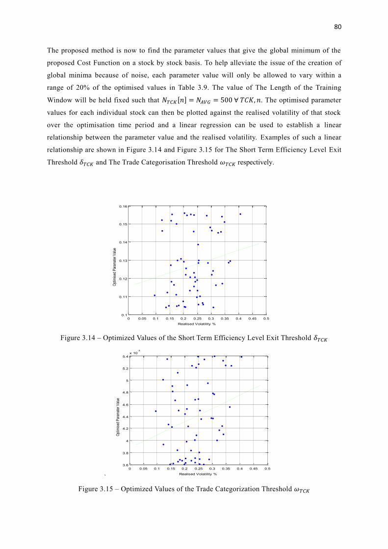
80

The proposed method is now to find the parameter values that give the global minimum of the

proposed Cost Function on a stock by stock basis. To help alleviate the issue of the creation of

global minima because of noise, each parameter value will only be allowed to vary within a

range of 20% of the optimised values in Table 3.9. The value of The Length of the Training

Window will be held fixed such that 𝑁𝑇𝐶𝐾[𝑛] = 𝑁𝐴𝑉𝐺 = 500 ∀ 𝑇𝐶𝐾, 𝑛. The optimised parameter

values for each individual stock can then be plotted against the realised volatility of that stock

over the optimisation time period and a linear regression can be used to establish a linear

relationship between the parameter value and the realised volatility. Examples of such a linear

relationship are shown in Figure 3.14 and Figure 3.15 for The Short Term Efficiency Level Exit

Threshold 𝛿𝑇𝐶𝐾 and The Trade Categorisation Threshold 𝜔𝑇𝐶𝐾 respectively.

Figure 3.14 – Optimized Values of the Short Term Efficiency Level Exit Threshold 𝛿𝑇𝐶𝐾

`

Figure 3.15 – Optimized Values of the Trade Categorization Threshold 𝜔𝑇𝐶𝐾

0 0.05 0.1 0.15 0.2 0.25 0.3 0.35 0.4 0.45 0.50.1

0.11

0.12

0.13

0.14

0.15

0.16

Realised Volatility %

Opt

imis

ed P

aram

ater

Val

ue

0 0.05 0.1 0.15 0.2 0.25 0.3 0.35 0.4 0.45 0.53.6

3.8

4

4.2

4.4

4.6

4.8

5

5.2

5.4x 10

-3

Realised Volatility %

Opt

imis

ed P

aram

ater

Val

ue

81

It should be noted that in Figure 3.14 and Figure 3.15 only points for which the optimised value

of the proposed Cost Function is less than zero have been plotted and for all parameters the

linear regression fit would only be based on such points, the purpose for this is to prevent poorly

optimised or unsuccessfully optimised data points from adversely affecting the regression. From

Figure 3.14 and Figure 3.15 the wide distribution of points around the linear regression lines can

be clearly seen, such a distribution illustrates the influence of noise in determining the optimal

parameter values. The use of a regression fit has an effect of averaging such noise across a

universe of stocks. It may then be seen that a parameter value taken from the regression

(average) line have a more rational basis for use than the actual optimised value for any

particular stock. The trend of increasing parameter values with increasing stock volatility does

make intuitive sense. Increasing volatility would correspond to an increasing standard deviation

of the stock price returns over any time period and a wider distribution of returns. A wider

distribution of returns would correspond to the requirement of larger classification boundaries

corresponding to a larger value of 𝜔𝑇𝐶𝐾. A wider distribution of returns would also correspond to

larger stock price movements being required for the end of any detected Overreaction Anomaly or

Momentum Anomaly to occur and this would correspond to a larger value of 𝛿𝑇𝐶𝐾.

Thus far all optimisation has been carried out using only Test Set 2 as an Optimisation Data Set.

The established relationships between parameter values and realised volatility would allow

suitable parameter values to be determined for use in proceeding Data Sets without the need for

computationally intensive optimisations, since the historical realised volatility of any stock can

be easily determined. The established relationships would also allow suitable parameter values

to be determined for stocks that are not part of the Optimisation Data Set. The success of the

proposed method is demonstrated in the next section.

3.6 Testing The Proposed Method

In this section testing results are presented to show the performance of the proposed novel

Neural Network framework. The chosen measure for performance is the Average Annualised

Information Ratio (Equation 3.8) across an initial Testing Stock Universe of the same 100 stocks

used to generate the results shown in Table 3.7. Performance will be tested across Test Set 2 to

Test Set 7 as shown in Table 3.7. The Annualised Information Ratio is equivalent to the ratio of

Annual Full Participation P&L to Annual Full Participation Volatility and the average of The

Annualised Information Ratio then represents the average risk weighted performance that could

be achieved under the assumption that such average trading opportunities could be found at each

instance in time. The assumption that such average trading opportunities could be found at each

point in time is a reasonable one when the underlying universe of stocks is large. Testing results

82

are shown in Table 3.10 and are inclusive of Transaction Costs 𝑡𝑇𝐶𝐾[𝑚] = 0.04% ∀ 𝑇𝐶𝐾,𝑚 per

trade. It should be noted that only those stocks for which a non-zero number of trades were

generated in any particular test set have been included in the computation of averages.

As a benchmark for performance the Average Annualised Information Ratio of a passive investment

into SPX INDEX is also presented for each Test Set in Table 3.8. From the results in can be seen that

the proposed framework has achieved a higher Information Ratio than the SPX INDEX over 4 of the

6 data Test Sets. From the proposed framework Test Set 2 had been used for parameter optimisation

and as such may now not be considered a valid data test set. Considering then just the five last data

test sets (Test Set 3 to Test Set 7 inclusive) it can be seen that the proposed framework has achieved

an average Information Ratio of 1.359 compared to 0.633 for SPX INDEX, this represents a risk

weighted performance improvement of around 115%.

It should be noted that the risk weighted performance as represented by the Average Annualised

Information Ratio is a measure based upon effectively selecting at any point in time a single stock that

has a risk weighted performance equivalent to the Average Annualised Information Ratio. However if

at any point in time several such stocks are combined into a Portfolio then the expected Annualised

Information Ratio of such a Portfolio would be higher than for a single stock alone and as such

through the creation of Portfolios higher Risk Weighted Returns can be achieved. The creation of

trading Portfolios forms the subject matter of the next Chapter of this Thesis.

As a validation check a second set of 100 stocks is now considered. The original stock sub-universe

consisted of the 4th

, 8th

, 12th

, .. , 400th

largest stocks taken from a universe of 447 out of 500 of

the current constituents of SPX INDEX. A second stock sub-universe is formed from the 3rd

, 7th

,

11th

, .. , 399th

largest stocks taken from the same universe of 447 out of 500 of the current

constituents of SPX INDEX. There are no overlapping stocks between the two sub-universes.

The regenerated performance results are shown in Table 3.11 for this second stock sub-universe.

The results of Table 3.11 have been produced without any additional parametric optimisation

since the regression fitted straight lines produced using Test Set 2 of the original

stock sub-universe can now be used for this second stock sub-universe. A comparison of the

Measure Test Set 2 Test Set 3 Test Set 4 Test Set 5 Test Set 6 Test Set 7

Testing Start 21/05/07 16/05/08 14/05/09 12/05/10 09/05/11 04/05/12

Testing End 16/05/08 14/05/09 12/05/10 09/05/11 04/05/12 06/05/13

Avg. Ann. Inf. Ratio 2.060 1.529 1.427 1.280 1.954 0.604

SPX Inf. Ratio -0.330 -0.827 1.749 0.912 0.073 1.258

Table 3.10 - Average Performance Figures for an Optimized Neural Network Framework

83

Measure Test Set 2 Test Set 3 Test Set 4 Test Set 5 Test Set 6 Test Set 7

Testing Start 21/05/07 16/05/08 14/05/09 12/05/10 09/05/11 04/05/12

Testing End 16/05/08 14/05/09 12/05/10 09/05/11 04/05/12 06/05/13

Avg. Ann. Inf. Ratio 0.737 1.115 1.192 1.755 2.120 1.177

SPX Inf. Ratio -0.330 -0.827 1.749 0.912 0.073 1.258

Table 3.11 - Average Performance Figures for a Second Set of Stocks

results of Table 3.11 with those of Table 3.10 shows that there has been no performance

degradation in moving to an independent stock sub-universe and this should provide comfort

that the original parametric optimisation approach has not introduced overfitting.

3.7 Summary

In this Chapter a novel framework for Trading Opportunity (trend) Detection has been presented.

The framework is built directly upon the detection of Overreaction and Momentum anomalies

under the premise that at most times any particular stock should be seen as efficiently priced.

The detection of Overreaction and Momentum anomalies is based on a novel combination of just

two Technical Analysis metrics, the Short Term Efficiency Indicator and the Average Efficienc y

Indicator. As a starting point it has been shown that these two metrics could be used to create a

profitable trading strategy without the application of any advanced Machine Learning

techniques. This is an important step as it shows that the eventual development of any Neural

Network based trading strategy would have an economically rational underlying foundation.

It was then shown that the two Efficiency Indicator metrics could be applied as Input Features to

a Neural Network based system for the detection of trading anomalies, although with limited

initial success. The first step has been to try and simply throw data at the Neural Network and it

is clear that there needed to be some further element of system design. Following this the Neural

Network method has been improved through the introduction of an expanded trade classification

scheme that would allow for the classification of Outliers in the data. Two novel heuristic

regularisation methods have also been presented. The first heuristic regularisation method is

termed Zero Appending and involves placing artificial biasing data points into a Training Set to

deal with the issue that a Training Set will typically not span the complete Feature Space. The

second heuristic regularisation method is termed Neural Network Output Smoothing and

provides a method to deal with noise in Neural Network output for any of piece of Test Data.

A novel method for parametric optimisation has also been presented. The optimisation technique

involves an initial global search for optimal parameters across a universe of stocks. Optimal

84

parameters on a stock by stock basis are then determined by allowing some constrained

movement from the globally optimal parameters. However, it is a regression of these individual

stock parameters as a function of realised volatility that eventually leads to the true optimised

parameters. Such a method allows for the smoothing of noise and also introduces computational

efficiency as the optimised parameters for any stock that is not part of the optimisation dataset

can be estimated with just knowledge of the recent realised volatility of that stock. Through

testing results it has been shown that the parametric optimisation technique has not introduced

overfitting. Testing results have been presented across a wide universe of stocks and across a

wide range of market conditions. The overall Neural Network framework has been shown to

have been successful throughout, even with the inclusion of Transaction Costs.

The detection of trading opportunities is not in itself sufficient to begin trading. The detected

trading opportunities need to be combined together to form a Portfolio. The choice and

weighting of trading opportunities into a trading Portfolio is an interesting challenge. Standard

Portfolio Construction techniques are not well suited for the creation of Portfolios that are based

upon the expectation of the reversal of short term trading anomalies. In the next Chapter a novel

method for Portfolio Construction under such conditions is presented.

85

Chapter 4

A New Graphical Model Framework For Dynamic Equity

Portfolio Construction

In this Chapter the development of a novel framework for Portfolio Construction under dynamic

environments is presented. The Chapter begins with an Introduction to highlight the motivation

behind the development of the framework. The introduction is followed by the establishment of a

performance benchmark through a simple approach to Portfolio Construction with application to the

Neural Network framework of the previous Chapter. The application of standard Mean-Variance

techniques for Portfolio Construction is then considered and it is shown that such methods are not

suited to the Neural Network framework. A novel method for Portfolio Construction is then presented

and a novel Genetic Algorithm optimisation technique is also introduced. Back testing results are

presented to demonstrate the performance of the framework. The Chapter ends with a summary.

4.1 Introduction

In the previous Chapter a technique for finding long and short trading opportunities based on a search

for Momentum and Overreaction anomalies has been presented. It has been shown through the results

presented in Table 3.10 and Table 3.11 that the proposed technique has been able to consistently find

profitable trading opportunities over a test period of 6 years. The results presented in Table 3.10 and

Table 3.11 consider an average stock drawn from each of two test universes of 100 stocks. In Figure

4.1 and Figure 4.2, overleaf, the Cumulative Distribution Function (CDF) of the number of Buy and

Sell signals generated on each day for the same stock universe used to generate Table 3.10 is

presented. From Figure 4.1 and Figure 4.2 it can be seen that with a probability of around 60% on any

given trading day there will be more than one Buy and Sell signal generated from the novel Neural

Network framework of the previous Chapter. This then presents a Portfolio Construction problem.

Given a fixed pool of investment cash, how should that cash be allocated amongst the two or more

stocks to form an optimised Portfolio?

In Chapter 2 a number of techniques of Portfolio Construction have been presented from the wider

literature. Such Portfolio Construction techniques are typically based upon Mean-Variance

optimisation and it has been discussed in Chapter 2 that such techniques place an assumption that the

distribution of asset returns falls into the Elliptical Family of probability distributions, whose

members include the Normal and Student-t Distributions. In addition it has been shown in Chapter 2,

through an empirical example, that the Portfolio weights generated by Mean-Variance Portfolio

86

Figure 4.1 – CDF of Number of Buy Trades Generated per Day for a First Sample of 100 Stocks

Figure 4.2 – CDF of Number of Sell Trades Generated per Day for a First Sample of 100 Stocks

techniques are highly sensitive to the values of the input parameters used. In addition Mean-Variance

Portfolio construction techniques are generally intended to be used for the creation of long term stable

Portfolios. The current problem of interest is for a much more dynamic trading environment. In the

current case of interest Portfolios are being created for a holding period of just one day and for such

cases Mean-Variance optimisation may not be well suited.

In this Chapter a novel method for Portfolio Construction that is specifically designed for dynamic

trading environments is presented. The method places no distributional assumptions upon the returns

of each of the assets used to form the Portfolio and it will be shown that the method is not unstably

sensitive to the values of the input parameter used. In the next subsection a simple benchmark against

0 5 10 15 20 25 30 350

0.2

0.4

0.6

0.8

1

x

F(x

)

Empirical CDF

0 5 10 15 20 25 300

0.2

0.4

0.6

0.8

1

x

F(x

)

Empirical CDF

87

which the new proposed method can be tested is presented. This is followed by an analysis of Mean-

Variance optimisation and its application to trading signals generated by the Neural Network

framework of the previous Chapter. In the subsections that follow a new proposed method is

introduced and then enhanced. Extensive back testing is conducted to show that the proposed method

would have outperformed the established benchmark across a wide universe of stocks.

4.2 Simple Approach to Portfolio Construction, Beating the Index

As a motivation for this Thesis it had been stated that most human analysts fail to consistently beat the

performance of benchmark Equity Indices. This created a motivation to conduct research to explore

the application of Machine Learning. In the previous Chapter a technique for finding long and short

trading opportunities based on a search for Momentum and Overreaction anomalies has been

presented. It has been shown that the proposed technique has been able to consistently find profitable

trading opportunities over a test period of 6 years. Two example test universes of 100 stocks have

been considered in the previous Chapter and it has been shown that typically more than one Buy or

Sell trading signal is generated per day from the potential 100 trading signals.

Consider the case of a Long Only Portfolio which will only Buy into stocks. A suitable industry

standard benchmark for such a Portfolio is the Standard and Poors 500 Index (Bloomberg Code: SPX

INDEX). A simple technique that could be applied to the Neural Network framework of the previous

Chapter would be to divide the available capital equally amongst those stocks which are signalling

Buy trades on any day. The results of the application of such a Portfolio Construction technique to the

two test universes of 100 stocks, as considered in Chapter 3, are shown in Figure 4.3 and Figure 4.4.

Figure 4.3 – Portfolio Levels Against Benchmarks for a First Sample of 100 Stocks

07 08 09 10 11 1250

100

150

200

250

300

350

400

Date

Port

folio

Level U

SD

Proposed

Eq. Wgt. Bskt.

SPX INDEX

88

Figure 4.4 – Portfolio Levels Against Benchmarks for a Second Sample of 100 Stocks

Each of the Figures is based on an investment of 100 USD in April 2006 with investment on each

subsequent trading day of 100 USD plus any accumulated profits and losses since April 2006. The

‘Proposed’ Portfolio is that based upon the Neural Network framework of the previous Chapter with

an equal division of Portfolio assets into those stocks that Signal a Buy trade on any particular trading

day. In each Figure the SPX INDEX benchmark is shown alongside a second benchmark which is an

Equally Weighted Basket of the universe of 100 stocks formed in April 2006 with no subsequent

rebalancing of the basket. From the two figures it can be seen that for two example cases the proposed

method has been able to form a Portfolio that is capable of consistently beating the benchmark SPX

INDEX. Therefore for two example cases it has been shown that a Machine Learning based method

has been able to achieve something that the average human analyst could not.

At this stage a Portfolio Construction benchmark has been established in the form of an equal division

of funds amongst the signalled Buy trades from the Neural Network framework of the previous

Chapter. Throughout the rest of this Chapter a novel method for Portfolio Construction will be

developed and it will be shown that such a novel method is able to outperform this recently

established benchmark across a wider universe of stocks.

4.3 Application of Current Portfolio Methods, Room For Improvement

The issue of Portfolio optimisation has received much attention in the literature with the standard

methods being based on Mean-Variance optimisation. For a universe of 𝑁 stocks such techniques

require as inputs 𝑁 estimates of Expected Return, 𝑁 estimates of Variance and 𝑁∙(𝑁−1)

2 estimates of

07 08 09 10 11 1240

60

80

100

120

140

160

180

200

220

240

Date

Port

folio

Level U

SD

Proposed

Eq. Wgt. Bskt.

SPX INDEX

89

Correlation. Estimates of such parameters are typically based upon historical data. The premise

of the Neural Network framework of interest is that the framework is able to detect the existence

of Momentum or Overreaction anomalies. If a Mean-Variance Portfolio Construction technique

were to be employed the natural question that arises is whether parameter estimates should be

based upon the entire available duration of historical data or just upon those in-situ data points at

which a trading signal (anomaly) has been generated by the Neural Network framework. Using

all available historical data would give more data points upon which to base historical estimates

and therefore it might be expected that this would lead to higher quality parameter estimates .

However the underlying premise is the detection of anomalies and as such for any given stock

the distribution of returns for those in-situ time periods at which an anomaly has been detected

would be expected to be different to the distribution of returns over the complete set of historical

data. Indeed, given that the problem at hand is the formation of a Portfolio of stocks for which

anomalies have been detected there then seems to be a compelling argument to base parameter

estimates only upon such in-situ historical data.

However, the use of only in-situ historical data introduces an additional problem. Table 4.1

shows the number of Buy trade signals generated over a six year period for a subset of stock

pairs from the same universe of 100 stocks used to generate Figure 4.3. The leading diagonal

show the number of trades generated for each single stock from a possible 1500 trades and the

off-diagonal entries show the number of trades generated for particular stock pairs. The use of

Mean-Variance optimisation techniques requires a full specification of the 𝑁∙(𝑁−1)

2 pairs of a

Correlation Matrix of the returns of 𝑁 assets. However, as can be seen from Table 4.1, for many stock

pairs the number of coincidental in-situ trades that occur at the same time for any two stocks is very

low and in some cases this number is zero. Over the complete set of historical data the average

number of times that any specific pair of stocks have signalled Buy trades on the same day is 3.50

Table 4.1 – Number of Trades Generated for a Subset of Stock Pairs over a Six Year Period

STOCK 91 92 93 94 95 96 97 98 99 100

91 103 4 3 17 8 26 32 6 5 12

92 44 2 2 0 13 3 7 1 4

93 18 5 1 4 5 10 3 2

94 64 8 17 20 6 4 3

95 28 11 9 3 3 1

96 186 28 10 24 14

97 124 11 12 16

98 41 7 0

99 82 9

100 86

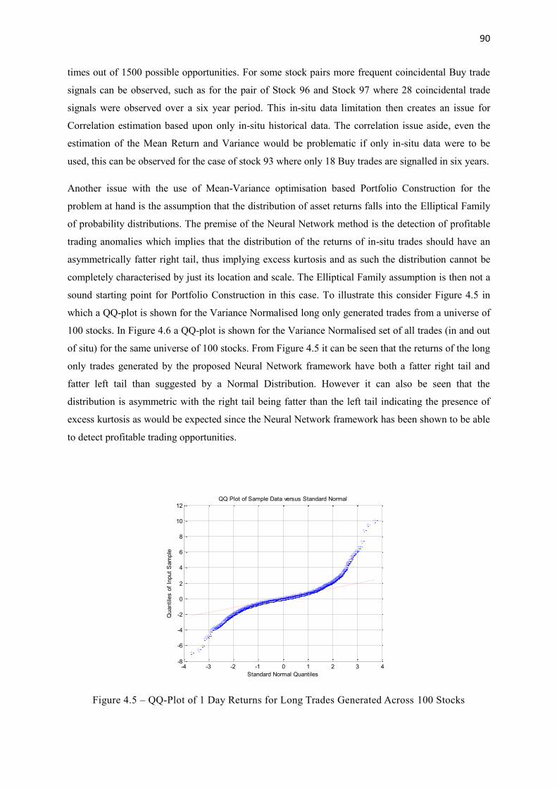
90

times out of 1500 possible opportunities. For some stock pairs more frequent coincidental Buy trade

signals can be observed, such as for the pair of Stock 96 and Stock 97 where 28 coincidental trade

signals were observed over a six year period. This in-situ data limitation then creates an issue for

Correlation estimation based upon only in-situ historical data. The correlation issue aside, even the

estimation of the Mean Return and Variance would be problematic if only in-situ data were to be

used, this can be observed for the case of stock 93 where only 18 Buy trades are signalled in six years.

Another issue with the use of Mean-Variance optimisation based Portfolio Construction for the

problem at hand is the assumption that the distribution of asset returns falls into the Elliptical Family

of probability distributions. The premise of the Neural Network method is the detection of profitable

trading anomalies which implies that the distribution of the returns of in-situ trades should have an

asymmetrically fatter right tail, thus implying excess kurtosis and as such the distribution cannot be

completely characterised by just its location and scale. The Elliptical Family assumption is then not a

sound starting point for Portfolio Construction in this case. To illustrate this consider Figure 4.5 in

which a QQ-plot is shown for the Variance Normalised long only generated trades from a universe of

100 stocks. In Figure 4.6 a QQ-plot is shown for the Variance Normalised set of all trades (in and out

of situ) for the same universe of 100 stocks. From Figure 4.5 it can be seen that the returns of the long

only trades generated by the proposed Neural Network framework have both a fatter right tail and

fatter left tail than suggested by a Normal Distribution. However it can also be seen that the

distribution is asymmetric with the right tail being fatter than the left tail indicating the presence of

excess kurtosis as would be expected since the Neural Network framework has been shown to be able

to detect profitable trading opportunities.

Figure 4.5 – QQ-Plot of 1 Day Returns for Long Trades Generated Across 100 Stocks

-4 -3 -2 -1 0 1 2 3 4-8

-6

-4

-2

0

2

4

6

8

10

12

Standard Normal Quantiles

Quantile

s o

f In

put

Sam

ple

QQ Plot of Sample Data versus Standard Normal

91

Figure 4.6 – QQ-Plot of 1 Day Returns for All Returns Generated Across 100 Stocks

The results of Figure 4.5 provide further support against the use of a Portfolio Construction technique

which assumes that the distribution of returns falls into the Elliptical Family. For comparison a QQ-

plot for all of the one-day returns, considering both in and out of situ data, is presented in Figure 4.6.

From Figure 4.6 it can be seen that for all returns considered together there is both a fatter right and

left tail than implied by a Normal Distribution, however there is little visual presence of excess

kurtosis. The returns as shown in Figure 4.6 could perhaps be captured by a Student-t distribution.

To further demonstrate the issues consider the application of Mean-Variance based optimisation to

just a two stock Portfolio of Stock 96 and Stock 97. The case where parameters are estimated based

on all available data is considered in Figures 4.7 to 4.10 below.

Figure 4.7 – Rolling Annualised One Business Day Historical Return for Example Stocks

-5 -4 -3 -2 -1 0 1 2 3 4 5-30

-20

-10

0

10

20

30

40

50

Standard Normal Quantiles

Quantile

s o

f In

put

Sam

ple

QQ Plot of Sample Data versus Standard Normal

08 09 10 11 12-0.8

-0.6

-0.4

-0.2

0

0.2

0.4

0.6

0.8

1

1.2

Date

Annualis

ed 1

Day R

etu

rn

Stock 96

Stock 97

92

Figure 4.8 – Rolling Annualised Volatility for Example Stocks

Figure 4.9 – Rolling 260 Business Day Realized Correlation for Two Example Stocks

Figure 4.10 – Percentage Allocation to Example Stocks Based on Sharpe Ratio Optimization

08 09 10 11 120.2

0.3

0.4

0.5

0.6

0.7

0.8

0.9

1

Date

Annualis

ed 1

Day S

tandard

Devia

tion

Stock 96

Stock 97

08 09 10 11 120

0.1

0.2

0.3

0.4

0.5

0.6

0.7

Date

Rolli

ng 2

60 D

ay C

orr

ela

tion

Correlation Stocks 96/97

Jul10 Aug10-0.2

0

0.2

0.4

0.6

0.8

1

Date

Sto

ck W

eig

hts

Weight Stock 96, Weight Stock 97

93

From these figures the instability of the estimated Mean Return (Figure 4.7), Annualised Volatility

(Figure 4.8) and Correlation (Figure 4.9) can be clearly seen, parameters are based on rolling 260

business day windows. The weights of the Sharpe Ratio optimised Portfolio at some of the points

where both Stock 96 and Stock 97 have coincidentally signalled Buy trades are shown in Figure 4.10.

From Figure 4.10 the instability in the optimised weights can be clearly seen, Sharpe Ratio Portfolio

optimisation is implying a 100% investment in one or other of the two assets with the choice flipping

in just a short period of time. There are clear stability issues with Mean-Variance optimisation.

The case where parameters are estimated based on only in-situ data is considered in Figures 4.11 to

4.14. From these figures the continued instability of the estimated Mean Return (Figure 4.11),

Annualised Volatility (Figure 4.12) and Correlation (Figure 4.13) can be clearly seen, parameter

estimates are based on all available in-situ historical data up to the estimation date. The weights of the

Sharpe Ratio optimised Portfolio at some of the 28 points where both Stock 96 and Stock 97 have

coincidentally signalled Buy trades are shown in Figure 4.14. From Figure 4.14 the continued

instability in the optimised weights can be clearly seen, Sharpe Ratio Portfolio optimisation is

implying a close to 100% investment in one of the two assets. The allocation makes intuitive sense

since Stock 97 has a higher historical return and lower historical volatility than Stock 96 based on the

estimation method that is employed. Although it is clear that such an allocation may arise in a Mean-

Variance based framework, there would be some expected value to diversification and it appears that

this value is lost in the optimisation. An alternative to Mean-Variance optimisation is clearly needed.

Figure 4.11 – Rolling Annualised In-Situ One Business Day Returns for Example Stocks

01/01/05 07/02/07 01/01/10 07/02/12-8

-6

-4

-2

0

2

4

6

8

Date

Annualis

ed 1

Day R

etu

rn

Stock 96, Stock 97

94

Figure 4.12 – Rolling Annualised In-Situ Volatility for Example Stocks

Figure 4.13 – Rolling In-Situ Realized Correlation for Two Example Stocks

Figure 4.14 – Percentage Allocation to Example Stocks Based on Sharpe Ratio Optimization

01/01/05 07/02/07 01/01/10 07/02/120

0.2

0.4

0.6

0.8

1

1.2

1.4

Date

Annualis

ed 1

Day S

tandard

Devia

tion

Stock 96, Stock 97

01/01/10 01/01/11

0.65

0.7

0.75

0.8

0.85

0.9

0.95

1

Date

Rolli

ng 2

60 D

ay C

orr

ela

tion

Stock 96, Stock 97

Jul10 Aug10-0.2

0

0.2

0.4

0.6

0.8

1

Date

Sto

ck W

eig

hts


95

4.4 A Novel Method for Portfolio Construction

In this section a novel method for Portfolio Construction is presented. The method overcomes the

limitations of Mean-Variance based Portfolio Construction techniques. The method places no strong

requirements that the distributions of asset returns fall into any special family of distributions. The

method is also designed to be used in environments where little data is available in order to form

parameter estimates and as such the method is well suited to the formation of Portfolios based on

trading signals from the Neural Network framework.

The inspiration for the method is The Google Page Rank algorithm and a brief overview of this is

presented first. A simplified Markov Chain model of the internet based on the existence of just 4 web

pages, each of which has some search keyword in the text body, is shown in Figure 4.15 below. In this

model there is a hypothetical web user bouncing around between the different pages. The user may be

in one of 4 states {S1,S2,S3,S4} where one of the four pages is being viewed. A discrete time

framework is considered and the probability distribution of the viewing location of the user at

timestamp 𝑚 can be given as

𝑄[𝑚] = [𝑄1[𝑚],𝑄2[𝑚],𝑄3[𝑚], 𝑄4[𝑚]]𝑇 (4.1)

where 𝑄1[𝑚], 𝑄2[𝑚],𝑄3[𝑚], 𝑄4[𝑚] are the probabilities that the user is in state S1, S2, S3 and

S4 respectively at timestamp 𝑚. Since 𝑄[𝑚] represents a distribution it must be the case that

Figure 4.15 – A Simplified Model of the Internet with Just 4 Web Pages

96

𝑄𝑇[𝑚] = 1 (4.2)

where is a Column Vector of Ones of the same length as 𝑄[𝑚], this is so say that the sum of the

elements of 𝑄[𝑚] must be one. At each timestamp the user is able to transition from their current

page to any of the other four pages or to stay on the current page. The probability of transition from a

Page A to another Page B is specified as 𝑃{𝐴,𝐵} and the complete set of transition probabilities is given

by the Transition Matrix

ℙ =

[ 𝑃{1,1} 𝑃{2,1} 𝑃{3,1} 𝑃{4,1}𝑃{1,2} 𝑃{2,2} 𝑃{3,2} 𝑃{4,2}𝑃{1,3} 𝑃{2,3} 𝑃{3,3} 𝑃{4,3}𝑃{1,4} 𝑃{2,4} 𝑃{3,4} 𝑃{4,4}]

(4.3)

It is a requirement that each of the columns of ℙ must sum to one since from any Page A the user

must transition to one of the 4 pages that make up this hypothetical internet. Given the distribution

𝑄[𝑚], the distribution of the viewing location at the next time 𝑚 + 1 can then be calculated as

𝑄[𝑚 + 1] = ℙ𝑄[𝑚] (4.4)

Here it is assumed that the Markov property holds such that the probability distribution at timestamp

𝑚 + 1 is directly dependent only upon the state of the system at timestamp 𝑚 and is not

influenced by how the state at timestamp 𝑚 had arisen. The Markov property states that the past

and the future are conditionally independent given the present. Over the long run the Markov

Chain would be expected to converge to a stationary distribution 𝑄[∞] such that

𝑄[∞] = ℙ𝑄[∞] (4.5)

Equation 4.5 can be viewed as an Eigenvalue-Eigenvector problem. The stationary distribution can be

shown [114] to exist and be unique under the condition of strictly positive ℙ𝛼 for some 𝛼 > 0. The

Markov Chain is non-reducible and hence the value of 𝑄[∞] is not obtainable by simple inspection.

However the solution 𝑄[∞] can be found as the principle Eigenvector of ℙ, the computational

solution of which is of order 𝑂(𝑁3) with 𝑁 being the dimension of ℙ. Alternatively an approximate

solution to 𝑄[∞] can be found by initialising some 𝑄[0] and then ‘running the chain’ to some

subjective degree of convergence.

In a simplified version of the Google Page Rank algorithm the entries of ℙ are based upon the

assumption that at the next timestamp a user will move from their present page to any of the

connected pages with an equal probability, self-transitions have a probability of zero. Therefore the

97

Transition Matrix is based on the presence or absence of links. An additional teleportation matrix is

also used so that with some small probability a user will move from a page to any other random page.

An initialised vector 𝑄[0] is used and the chain is run to convergence to give an estimated 𝑄[∞].

The entries of 𝑄[∞] give the probabilities that the user will converge to certain web pages in a

steady state distribution and this can be used to Rank the pages in a keyword search. The original

Google Page Rank algorithm [115] incorporated further complexity beyond this simple presentation.

Now back to the problem at hand, how to form an optimised Portfolio for those stocks that are

signalling Buy trades at any instant in time. As an analogy to the Page Rank problem, consider an

investor who divides $1 of funds amongst 𝑁 assets and moves the funds between assets according

to some Transition Scores. Funds are moved until a steady state distribution of the $1 amongst

the 𝑁 assets has been achieved. This situation could be well modelled by a Markov Chain,

however there are two complications. The first complication is that in a simple universe that

consists of just Stock A and Stock B there is a correlation between the returns of the stocks and

as such a simple two state model will not capture important information present in the joint

distribution of the returns of the two stocks. The second complication is in how to determine the

Transition Scores, the situation is no longer as simple as counting outgoing web links.

To address the first complication the concept of a ‘Bridge Portfolio’ is introduced. A Bridge

Portfolio for Stock A and Stock B would be a Portfolio consisting of $0.50 invested into each of

the two stocks. If the statistics of the Bridge Portfolio can be captured then the joint statistics of

Stock A and Stock B would be captured. The chain can be formed such that transitions of funds

between Stock A and Stock B occur only through the Bridge Portfolio. For a general universe of

𝑁 stocks there would be a requirement for ∑ 𝑛𝑁𝑛=1 states in the Markov chain, this is in order to

allow the inclusion of all 𝑁∙(𝑁−1)

2 Bridge Portfolios in order to incorporate all possible stock pairs.

Even a modest case of 𝑁 = 20 stocks signalling Buy trades the dimensionality of the Transition

Matrix ℙ would be 210 × 210. However, if the chain can be constructed such that a Bridge

Portfolio is only considered for adjacent stocks in the list then the resulting chain could be

simplified. Consider a case of 𝑁 = 4 stocks, the complete Markov Chain with Bridge Portfolios

that consider each possible stock pair is as shown in Figure 4.16, there are 10 states and 34

possible transitions. A simplified Markov Chain model with a Bridge Portfolio only between

adjacent stocks is as shown in Figure 4.17, there are only 8 states and 24 possible transitions.

Each state {A,B} in Figure 4.16 and Figure 4.17 corresponds to a $0.50 investment into each of Stock

A and Stock B. Such that {S1,S1} is a $1 investment in Stock 1 and {S1,S2} is a $0.50 investment in

each of Stock 1 and Stock 2. The model is such that funds can only flow from a stock to another

through a Bridge Portfolio.

98

Figure 4.16 – A Complete Markov Chain Model for Portfolio Construction with 4 Stocks

The Transition Matrix of the simplified chain in Figure 4.17 can be specified as

ℙ =

[ 𝑃{11,11} 𝑃{12,11} 0 0 0 0 0 𝑃{14,11}𝑃{11,12} 𝑃{12,12} 𝑃{22,12} 0 0 0 0 0

0 𝑃{12,22} 𝑃{22,22} 𝑃{23,22} 0 0 0 0

0 0 𝑃{22,23} 𝑃{23,23} 𝑃{33,23} 0 0 0

0 0 0 𝑃{23,33} 𝑃{33,33} 𝑃{34,33} 0 0

0 0 0 0 𝑃{33,34} 𝑃{34,34} 𝑃{44,34} 0

0 0 0 0 0 𝑃{34,44} 𝑃{44,44} 𝑃{14,44}𝑃{11,14} 0 0 0 0 0 𝑃{44,14} 𝑃{14,14}]

(4.6)

99

Figure 4.17 – A Simplified Markov Chain Model for Portfolio Construction with 4 Stocks

The chain can be further simplified by removing the connection between {S1,S1} and {S1,S4} giving

a chain which remains irreducible as is it still possible to indirectly move from any state to any other

state. The resulting Transition Matrix can be then be simplified to

100

ℙ =

[ 𝑃{11,11} 𝑃{12,11} 0 0 0 0 0 0

𝑃{11,12} 𝑃{12,12} 𝑃{22,12} 0 0 0 0 0

0 𝑃{12,22} 𝑃{22,22} 𝑃{23,22} 0 0 0 0

0 0 𝑃{22,23} 𝑃{23,23} 𝑃{33,23} 0 0 0

0 0 0 𝑃{23,33} 𝑃{33,33} 𝑃{34,33} 0 0

0 0 0 0 𝑃{33,34} 𝑃{34,34} 𝑃{44,34} 0

0 0 0 0 0 𝑃{34,44} 𝑃{44,44} 𝑃{14,44}0 0 0 0 0 0 𝑃{44,14} 𝑃{14,14}]

(4.7)

The format of the Matrix in Equation 4.7 is as a Tri-diagonal matrix, this is to say that it has nonzero

elements only on the main diagonal, as well as on the first diagonal below and the first diagonal above

the main diagonal. A property of such a matrix is that a Tri-diagonal Matrix Algorithm can be used to

solve the Eigen-System with just 𝑂(𝑁) operations. Such a Tri-diagonal matrix can also be stored

compactly in an 𝑁 × 3 format. Having now formed a structure that is compact in representation

and that would capture the joint statistics between a pair of stocks, the issue of how to score a

transition between two states can be addressed.

It is preferred to take an approach that places no distributional assumptions on the underlying

data. A frequency table of the discretised returns of each two stock Portfolio represented by a

state {A,B} can be initialised and each such frequency table can be updated based on in-situ trades for

the two stocks as they arise. Each frequency table is based on 51 buckets with the 𝑗𝑡ℎ bucket

corresponding to a single period return 𝑅𝑗 in the range

−5%+ (𝑗 − 1) × 0.2% < 𝑅𝑗 ≤ −5%+ 𝑗 × 0.2% (4.8)

As such each bucket represents the occurrence of a single period return in a range of 0.20% (20

basis points) and the buckets cover the closed range (−5.00%, 5.00%]. To allow for single

period returns outside of this range the leftmost bucket (bucket 1) is modified to the range

(−∞,−4.80%] and the rightmost bucket (bucket 51) is modified to the range (4.80%,∞). Each

frequency table can be initialised according to some prior belief of the distribution of returns if

such a belief is available. A simple alternative is to employ a ‘Laplace Estimator’ approach and

to initialise with a count of 1 in each bucket, it is this approach that will be employed.

Following initialisation, each frequency table is updated as coincidental in-situ trades arise for

the pair of stocks representing the state {A,B}. For a state {A,A} which represents only a single

stock A, the frequency table is updated each time an in-situ trade arises for Stock A. A frequency

table can be easily converted to a discrete distribution by simply dividing the frequency count in

each bucket by the total sum of frequency counts in all buckets. The formation of example

101

distributions for Stock 96 (distribution in state {96,96}), Stock 97 (distribution in state {97,97})

and the Bridge Portfolio of Stock 96 and Stock 97 (distribution in state {96,97}) are shown

below in Figure 4.18. The figure shows the discrete empirical distributions that are formed at

three different time points over a six year period.

The first row of images in Figure 4.18 shows the initialised distributions for the two stocks and for the

connecting ‘Bridge Portfolio’. In the second row of images the evolved distributions are shown as at

the final time point prior to the occurrence of a coincidental trade for Stock 96 and Stock 97, this is to

say that whilst Buy trades have been generated on each of the two stocks there have been no such

signals occurring at the same time for both stocks. The final row of images of Figure 4.18 shows the

distributions for the two stocks and for the ‘Bridge Portfolio’ at the end of the six year period.

Initialised Distribution of Returns for

Stock 96 (State {96,96})

Initialised Distribution of Returns for


Initialised Distribution of Returns for a

Bridge Portfolio (State {96,97})

Developing Distribution of Returns for


Developing Distribution of Returns for


Developing Distribution of Returns for a


Final Distribution of Returns for Stock

96 (State {96,96})

Final Distribution of Returns for Stock

97 (State {97,97})

Final Distribution of Returns for a


Figure 4.18 – Evolving Distributions for Two Example Stocks

-0.06 -0.04 -0.02 0 0.02 0.04 0.060

0.002

0.004

0.006

0.008

0.01

0.012

0.014

0.016

0.018

0.02

Discretised Return

Pro

babili

ty

-0.06 -0.04 -0.02 0 0.02 0.04 0.060

0.002

0.004

0.006

0.008

0.01

0.012

0.014

0.016

0.018

0.02

Discretised Return

Pro

babili

ty

-0.06 -0.04 -0.02 0 0.02 0.04 0.060

0.002

0.004

0.006

0.008

0.01

0.012

0.014

0.016

0.018

0.02

Discretised Return

Pro

babili

ty

-0.06 -0.04 -0.02 0 0.02 0.04 0.060

0.01

0.02

0.03

0.04

0.05

0.06

0.07

0.08

0.09

0.1

Discretised Return

Pro

babili

ty

-0.06 -0.04 -0.02 0 0.02 0.04 0.060

0.005

0.01

0.015

0.02

0.025

0.03

0.035

0.04

0.045

0.05

Discretised Return

Pro

babili

ty

-0.06 -0.04 -0.02 0 0.02 0.04 0.060

0.002

0.004

0.006

0.008

0.01

0.012

0.014

0.016

0.018

0.02

Discretised Return

Pro

babili

ty

-0.06 -0.04 -0.02 0 0.02 0.04 0.060

0.01

0.02

0.03

0.04

0.05

0.06

Discretised Return

Pro

babili

ty

-0.06 -0.04 -0.02 0 0.02 0.04 0.060

0.01

0.02

0.03

0.04

0.05

0.06

Discretised Return

Pro

babili

ty

-0.06 -0.04 -0.02 0 0.02 0.04 0.060

0.01

0.02

0.03

0.04

0.05

0.06

0.07

Discretised Return

Pro

babili

ty

102

At any given time the distributions that have been evolved up to that time can be used to score

transitions in the Graphical Model. A distribution can be converted to a Transition Score based upon a

number of possible criteria, for example the Expected Return or the ratio of Expected Return to

Standard Deviation could be determined from a distribution and either of these could be used as a

score. Such metrics would pose issues for the creation of a Long Only trading Portfolio as the score

would not be strictly positive, this could in turn lead to negative stock weights in a Portfolio. Such an

issue could be overcome by flooring the score at zero. However, a simpler and more robust scoring

method is to use the probability of a stock return being greater than some threshold. Such a method

would always guarantee a positive score and has a tractable economic basis. By moving trading funds

in the direction of positive returns this should help to achieve a Portfolio with a positive return,

additionally it should be expected to reduce Portfolio volatility as funds are continually being pushed

to that part of the joint distribution that has a positive return.

The transition scoring method then is to score transitions into a state {A,B} with the probability 𝑃{𝐴𝐵}

that the Bridge Portfolio of Stock A and Stock B has a return greater than a subjective threshold 𝑇,

this will be specified as 𝑃{𝐴𝐵} > 𝑇 . The resulting Transition Matrix is then

ℙ =

[ 𝑃{11} > 𝑇 𝑃{11} > 𝑇 0 0 0 0 0 0

𝑃{12} > 𝑇 𝑃{12} > 𝑇 𝑃{12} > 𝑇 0 0 0 0 0

0 𝑃{22} > 𝑇 𝑃{22} > 𝑇 𝑃{22} > 𝑇 0 0 0 0

0 0 𝑃{23} > 𝑇 𝑃{23} > 𝑇 𝑃{23} > 𝑇 0 0 0

0 0 0 𝑃{33} > 𝑇 𝑃{33} > 𝑇 𝑃{33} > 𝑇 0 0

0 0 0 0 𝑃{34} > 𝑇 𝑃{34} > 𝑇 𝑃{34} > 𝑇 0

0 0 0 0 0 𝑃{44} > 𝑇 𝑃{44} > 𝑇 𝑃{44} > 𝑇

0 0 0 0 0 0 𝑃{41} > 𝑇 𝑃{41} > 𝑇]

(4.9)

The columns of this matrix will not sum to one. The odd numbered rows of the Transition Matrix

would correspond to a transition of funds into a particular single stock and the even numbered rows

would correspond to a transition of funds into a Bridge Portfolio. Given one unit of investable money

this could be initially distributed in some chosen away amongst those 𝑁 stocks which are signalling

Buy trades. The initial distribution of funds would then be a vector of length 2𝑁 as follows

𝑄[0] = [𝑄11[0], 𝑄12[0], 𝑄22[0], 𝑄23[0], … , 𝑄𝑁𝑁[0], 𝑄𝑁1[0]]𝑇 (4.10)

where 𝑄𝐴𝐴[0] is the initial allocation of funds to Stock A and 𝑄𝐴𝐵

[0] = 0 ∀ 𝐴 ≠ 𝐵. It would be

the case that 𝑄[0]𝑇 = 1 such that the sum of the elements of 𝑄[0] is 1. The Transition Matrix

can then be used to move funds amongst the 𝑁 stocks and 𝑁 Bridge Portfolios such that

103

𝑄[1] =ℙ𝑄[0]

‖ℙ𝑄[0]‖ (4.11)

Where ‖∙‖2 is the Euclidean Norm Operator. The term ‖ℙ𝑄[0]‖ is required for Normalization since

the columns of ℙ no longer sum to one but the distribution of funds represented by 𝑄[1] must be

such that 𝑄𝑇[1] = 1 as the total invested funds must always remain as $1. The result in Equation

4.11 is then an updated distribution of the initial $1 of funds between the 𝑁 stocks and 𝑁 Bridge

Portfolios. Of interest is the long term equilibrium distribution of funds 𝑄[∞] and this can be

determined to be the normalised principle Eigenvector of ℙ. An alternative approach to determine

𝑄[∞] is to simply run the chain to convergence. Having determined an Equilibrium distribution

of funds 𝑄[∞] between the 𝑁 stocks and 𝑁 Bridge Portfolios all that remains is to reallocate the

funds in each Bridge Portfolio equally amongst those two stocks in the Bridge Portfolio.

In practice running the chain to convergence is seen to give an Equilibrium Portfolio within a

reasonable number of iterations. An example convergence diagram for a situation with 5 stocks

and 5 Bridge Portfolios is shown in Figure 4.19 below. The convergence of the Portfolio after

reallocation of the proceeds of the Bridge Portfolios is shown in Figure 4.20. The choice of a

Transition based on the probability of a positive single period return also leads to Portfolio

stability over adjacent time periods. Consider again the case of just two available stocks, Stock

96 and Stock 97, the allocation achieved by the proposed method over the same time points as in

Figure 4.14 is shown in Figure 4.21. There is clear stability of the Portfolio and this should be

expected as the created single stock and Bridge Portfolio distributions do not vary drastically

with each arriving in-situ data point. The proposed method has achieved diversification amongst

the two stocks as it is no longer the case of a near 100% allocation into just one stock.

Figure 4.19 – Convergence of the Distribution of Funds Amongst 5 Stocks and Bridge Portfolios

0 10 20 30 40 50 60 70 80 90 1000.02

0.04

0.06

0.08

0.1

0.12

0.14

0.16

Iteration

Weig

ht

in P

ort

folio

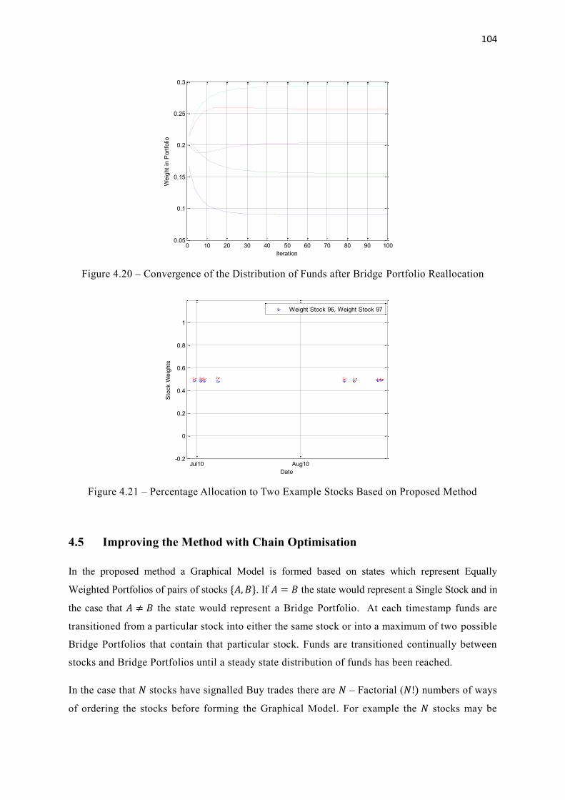
104

Figure 4.20 – Convergence of the Distribution of Funds after Bridge Portfolio Reallocation

Figure 4.21 – Percentage Allocation to Two Example Stocks Based on Proposed Method

4.5 Improving the Method with Chain Optimisation

In the proposed method a Graphical Model is formed based on states which represent Equally

Weighted Portfolios of pairs of stocks {𝐴, 𝐵}. If 𝐴 = 𝐵 the state would represent a Single Stock and in

the case that 𝐴 ≠ 𝐵 the state would represent a Bridge Portfolio. At each timestamp funds are

transitioned from a particular stock into either the same stock or into a maximum of two possible

Bridge Portfolios that contain that particular stock. Funds are transitioned continually between

stocks and Bridge Portfolios until a steady state distribution of funds has been reached.

In the case that 𝑁 stocks have signalled Buy trades there are 𝑁 – Factorial (𝑁!) numbers of ways

of ordering the stocks before forming the Graphical Model. For example the 𝑁 stocks may be

0 10 20 30 40 50 60 70 80 90 1000.05

0.1

0.15

0.2

0.25

0.3

Iteration

Weig

ht

in P

ort

folio

Jul10 Aug10-0.2

0

0.2

0.4

0.6

0.8

1

Date

Sto

ck W

eig

hts


105

Figure 4.22 – An Example Graphical Model Ordering

Figure 4.23 – An Alternative Graphical Model Ordering

kept in order such that the Graphical Model would be of the format of Figure 4.22. Alternatively,

the 𝑁 stocks could be arranged in some random order, resulting for example in a chain of the

format of Figure 4.23.

There is clearly scope for the use of optimisation techniques to find the most optimally ordered

chain. The issue of chain ordering can be seen as an equivalent issue of determining which

‘Bridge Portfolios’ should be used. In the case of 𝑁 stocks it must be the case that the set of 𝑁

states {{11}, {22},… , {𝑁𝑁}} would feature in the chain. However, the choice of which 𝑁 Bridge

Portfolios to feature would be a free choice subject to each of the 𝑁 stocks featuring in exactly

two Bridge Portfolios. It would make intuitive sense to form the most ‘confident chain’, this

would be the chain for which the most information is known about the connecting Bridge

Portfolios. A suitable metric then would be to order the stocks such that the total sum of the

number of data points in the resulting frequency tables of the constructed Bridge Portfolios

would be maximised.

The optimisation problem is then akin to a ‘Reverse Travelling Salesman Problem’. In the

classical Travelling Salesman Problem (TSP) an efficient salesman must start his journey in a

particular city (City A for example) and then visit each of a total of 𝑁 cities before returning

home to City A. The salesman being efficient wishes to complete his journey by covering the

lowest possible total distance and without visiting any particular city more than one time. The

problem is known to be NP-Hard (Non-Deterministic Polynomial Time Hard).

In the case of the Portfolio Optimisation Graphical Model problem of interest the number of data

points in the frequency table of a particular Bridge Portfolio {AB} of interest can be seen as

analogous to the distance between the stocks {A and B} when these stocks are thought of as

cities (City A and City B). The ordering of stocks in the Graphical Model can then be seen as a

106

‘Reverse Travelling Salesman Problem’, in this case the salesman wishes to collect Air Miles by

visiting a total of 𝑁 cities before returning home. The Air Mile collecting salesman then wishes

to complete his journey by covering the maximum possible total distance without visiting any

particular city more than one time. The problem remains NP-Hard.

There are known algorithms for finding exact solutions to the Travelling Salesman Problem and

these could perhaps be modified for the Reverse Travelling Salesman Problem of interest.

However in the case of the TSP it is known that Genetic Algorithm (GA) based optimisation

techniques can be used to find probably good solutions, although such solutions cannot be

proven to be optimal. Since for the application of interest it is not necessary to find the exact

optimal solution a GA based optimisation technique can be used.

The GA approach employed is to form initially a set of 100 random orderings of those 𝑁 stocks

which are signalling Buy Trades on any particular trading day. At each iteration the set of 100

orderings is subdivided randomly into 25 subsets of 4 orderings. Within each subset the best of

the 4 orderings is selected and then mutated through a set of random flips, swaps and slides to

give three new mutated orderings which when combined with the original best ordering gives a

new subset of 4 orderings. The recombination of these 25 sets of 4 orderings then creates a new

more optimised set of 100 orderings which can be used at the next iteration. The algorithm is run

until the best ordering at successive iterations has been observed to stabilise, such a stabilised

ordering is then used in the formation of the Graphical Model for Portfolio Optimisation.

Figure 4.24 – Convergence of Proposed GA Method for a Universe of 20 Stocks

0 20 40 60 80 100 120 140 160 180 200280

300

320

340

360

380

400

420

440

Iteration

Tota

l F

requency C

ount

107

Figure 4.25 – Convergence of Proposed GA Method for a Universe of 99 Stocks

The proposed GA based technique converges to a stabilised chain ordering within a reasonable

number of iterations. An example chain convergence for the case of 𝑁 = 20 stocks signalling

Buy trades at a particular instance in time is shown in Figure 4.24. Another example chain

convergence for the case of 𝑁 = 99 stocks signalling Buy trades at a particular instance in time

is shown in Figure 4.25. In the next section exhaustive simulations are shown to demonstrate the

proposed Portfolio Construction technique and in particular the improvement that can be gained

through the use of the proposed Optimisation technique for the ordering of stocks.

4.6 Testing the Proposed Method

In this section Monte Carlo type simulations are used to test the proposed method. To form a

testing universe the 500 constituents of the Standard and Poors 500 Index (Bloomberg Code:

SPX INDEX) as of May 2006 are taken and ordered by descending market capitalisation.

Simulations are carried out by selecting at random stocks from the complete universe of 500

stocks. For a first test, sub-universes of 100 stocks are created by choosing stocks at random

from the complete set of 500 stocks. For each sub-universe the Neural Network based Trading

Opportunity detection method of the previous Chapter is applied and this is followed by the

application of the Portfolio Construction Method developed in this Chapter. At each instance in

time a Portfolio is only created for those of the 100 stocks that are signalling a Buy trade at that

particular time based on the method proposed in Chapter 3. The Empirical CDF of the Terminal

Value based on an initial investment of 100 USD over a seven year time period from May 2006

to April 2013 is shown in Figure 4.26. The generated CDF is based on 1024 Monte Carlo

0 100 200 300 400 500 600 700 800 900 1000600

700

800

900

1000

1100

1200

1300

Iteration

Tota

l F

requency C

ount

108

Figure 4.26 – Empirical CDF of MC Simulation Results for Sub-Universes of 100 Stocks



0 200 400 600 800 1000 1200 1400 16000

0.1

0.2

0.3

0.4

0.5

0.6

0.7

0.8

0.9

1

x

F(x

)

Empirical CDF

Equally Weighted

Random Chain

Optimised Chain

0 200 400 600 800 1000 1200 1400 16000

0.1

0.2

0.3

0.4

0.5

0.6

0.7

0.8

0.9

1

x

F(x

)

Empirical CDF

Equally Weighted

Random Chain

Optimised Chain

0 200 400 600 800 1000 1200 1400 16000

0.1

0.2

0.3

0.4

0.5

0.6

0.7

0.8

0.9

1

x

F(x

)

Empirical CDF

Equally Weighted

Random Chain

Optimised Chain

109


simulations. Likewise, Monte Carlo Simulation results for sub-universes of 200, 300 and 400

stocks are shown in Figure 4.28, Figure 4.29 and Figure 4.30. From the it can be clearly seen

that the proposed method offers an improvement over an Equally Weighed approach to Portfolio

Construction, with a particularly marked improvement following the application of the GA based

Chain Optimisation technique. The scale of improvement can be seen to increase with an

increasing sub-universe size. This effect is rationalised by the fact that increasing the sub-

universe size increases the probability that more than one stock would be signalling a Buy trade

at any particular instance in time. As such there would be an increase in the probability that a

non-trivial multi-stock Portfolio can be optimised. The results are further summarised in Table

4.2 below where the Average Terminal value as of April 2013 based on an initial investment of

100 Dollars in May 2006 is shown for each of the different sub-universe sizes. In the case of a

sub-universe of 400 stocks it would be expected that an initial investment of 100 USD could be

grown to over 670 USD over a seven year period, this would represent a highly respected rate of

return. The use of a GA optimised chain gives an average performance increase of over 17%

compared to an Equally Weighed Portfolio; this is a highly respectable improvement.

Number of Stocks Equally Weighted Random Chain Optimized Chain

100 369.44 379.74 398.54

200 445.00 455.39 499.73

300 519.63 526.95 600.41

400 575.10 578.34 674.88

Table 4.2 - Average Terminal Values for Different Sub-Universe Sizes

0 200 400 600 800 1000 1200 1400 16000

0.1

0.2

0.3

0.4

0.5

0.6

0.7

0.8

0.9

1

x

F(x

)

Empirical CDF

Equally Weighted

Random Chain

Optimised Chain

110

4.7 Summary

In this Chapter a novel method for Portfolio Construction for application to the novel Neural

Network Framework of the previous Chapter has been presented. It had initially been shown that

an Equally Weighed Portfolio of those stocks which are signalling Buy Trade Opportunities

using the Neural Network Framework could outperform the benchmark SPX INDEX over a

significant period of time. The outperformance of a benchmark Equity Index was stated as a

motivation for this Thesis; however, there would always be further room for improvement by moving

beyond the Equally Weighted Portfolio.

The need for a new method for Portfolio Construction has been motivated through an analysis of

the short comings of current Mean-Variance based methods for Portfolio Construction when they

are applied to the Neural Network Framework. It has been shown that the returns of trades

generated by the Neural Network Framework are not well categorised by a distribution that falls

into the Elliptical Family due to the presence of a Fat Right Tail. As such an underlying

assumption of Mean-Variance based Portfolio methods has been violated. The need for a new

method has been further reinforced through the fact that coincidental in-situ trades for a pair of

stocks as generated by the Neural Network Framework occur rarely and hence the formation of

historic statistics as required for a Mean-Variance technique would be difficult.

The novel method presented in this Chapter overcomes the limitations of Mean-Variance based

Portfolio Construction techniques. The method places no strong requirement that the

distributions of asset returns fall into any special family of distributions, as such the method is

well suited to application with algorithms which select stocks exhibiting excess kurtosis in their

distribution of returns. The method is well suited to be used in environments where little data is

available to form parameter estimates. The novel method is based on a Graphical Model

Framework which has been shown to be computationally efficient to run to convergence. In

addition a Genetic Algorithm based optimisation technique has been shown to be effective in

optimising the Graphical Model and in dealing with data sparseness.

A back testing method based on a Monte Carlo selection of random stock universes of the

constituents of the Standard and Poors 500 Index (Bloomberg Code: SPX INDEX) has shown

that with the proposed method a significant improvement in performance beyond that which can

be achieved through an equally weighted Long Only Portfolio of those stocks which are

signalling a Buy Trade opportunity is possible. The performance is beyond that of the

benchmark SPX INDEX and hence it has been shown that though the application of Machine

Learning it has been possible to achieve something beyond the performance of the average

Active Equity Portfolio Manager.

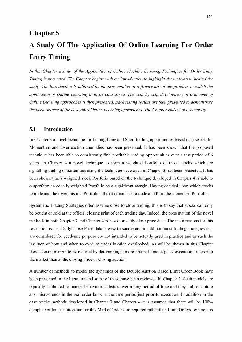
111

Chapter 5

A Study Of The Application Of Online Learning For Order

Entry Timing

In this Chapter a study of the Application of Online Machine Learning Techniques for Order Entry

Timing is presented. The Chapter begins with an Introduction to highlight the motivation behind the

study. The introduction is followed by the presentation of a framework of the problem to which the

application of Online Learning is to be considered. The step by step development of a number of

Online Learning approaches is then presented. Back testing results are then presented to demonstrate

the performance of the developed Online Learning approaches. The Chapter ends with a summary.

5.1 Introduction

In Chapter 3 a novel technique for finding Long and Short trading opportunities based on a search for

Momentum and Overreaction anomalies has been presented. It has been shown that the proposed

technique has been able to consistently find profitable trading opportunities over a test period of 6

years. In Chapter 4 a novel technique to form a weighted Portfolio of those stocks which are

signalling trading opportunities using the technique developed in Chapter 3 has been presented. It has

been shown that a weighted stock Portfolio based on the technique developed in Chapter 4 is able to

outperform an equally weighted Portfolio by a significant margin. Having decided upon which stocks

to trade and their weights in a Portfolio all that remains is to trade and form the monetised Portfolio.

Systematic Trading Strategies often assume close to close trading, this is to say that stocks can only

be bought or sold at the official closing print of each trading day. Indeed, the presentation of the novel

methods in both Chapter 3 and Chapter 4 is based on daily close price data. The main reasons for this

restriction is that Daily Close Price data is easy to source and in addition most trading strategies that

are considered for academic purpose are not intended to be actually used in practice and as such the

last step of how and when to execute trades is often overlooked. As will be shown in this Chapter

there is extra margin to be realised by determining a more optimal time to place execution orders into

the market than at the closing price or closing auction.

A number of methods to model the dynamics of the Double Auction Based Limit Order Book have

been presented in the literature and some of these have been reviewed in Chapter 2. Such models are

typically calibrated to market behaviour statistics over a long period of time and they fail to capture

any micro-trends in the real order book in the time period just prior to execution. In addition in the

case of the methods developed in Chapter 3 and Chapter 4 it is assumed that there will be 100%

complete order execution and for this Market Orders are required rather than Limit Orders. Where it is

112

the case that Market Orders are to be placed the issue is one of decision timing, at each instant in time

a decision should be made of whether to trade or to wait and in making such a decision it is really the

behaviour of the order book in the most recent time period that is relevant. The calibration of a

Double Auction Based Limit Order Book Model is a computationally intensive task and there simply

would not be sufficient time to recalibrate around any observed trends in the order book that are

evolving in the seconds preceding the decision of whether to trade now or to wait.

To help solve the problem there is available a toolbox of techniques of Online Machine Learning. In

the next section a more formalised framework of the problem at hand is presented, the section

presents the problem alongside the constraints that exist to find a solution. This is followed by the

presentation of the step by step development of a number of Online Machine Learning techniques for

Market Order Entry Timing, the techniques are analysed and compared against each other. In the

section that follows back test results are presented to demonstrate the performance of the approaches

across a large set of data. The Chapter ends with a summary.

5.2 Framework for the Order Execution Problem

In order to develop a framework for the Order Execution Problem consider Figure 5.1 below.

The Figure shows the evolution of the Best Bid Price for Verizon (Bloomberg Code: VZ

EQUITY) with samples taken at 15 second intervals for the 30 minute period prior to the closing

print of 3rd

March 2016. There are 4 points per one minute period with the final 120 points,

corresponding to the final 30 minutes of the normal trading session, being shown in green. The

24 point (6 minute) moving average of the Best Bid Price is shown as a Red Line. Verizon is a

highly liquid stock and the Best Ask Price was always 1 Cent (0.01 USD) above the Best Bid.

Figure 5.1 – Evolution of the Best Bid Price for Verizon

0 50 100 150 200 250 300 35051.65

51.7

51.75

51.8

51.85

51.9

51.95

Tick

Bid

Price

113

Consider now that the novel methods presented in Chapter 3 and Chapter 4 are modified such

that they are based on close to close data with the exception that for the current trading day the

stock prices at some period prior to the close are used as proxies for the closing prices of the

current trading day. This would then allow the weighted Portfolio of those stocks for which are a

trading opportunity has been detected to be formed prior to the closing print. If for example the

weighted Portfolio of stocks could be formed 30 minutes prior to the closing print and Verizon

was a stock which has been selected to be sold then a situation as depicted in Figure 5.1 would

arise. Verizon could then be sold at any of the green points, corresponding to the final 30

minutes of the trading session, the decision of whether to trade or not would need to be made

rapidly on a time point by time point basis. The trading decision can look back over the

preceding time interval. For example at the first green point (at time step 241) it is possible to

look back over the preceding 240 time points. At the first green point it can clearly be seen that

the 20 point moving average is an uptrend and hence by this metric it may be determined to be

advantageous not to sell Verizon at time point 241 but to wait and re-evaluate at time step 242.

To illustrate the use of a Moving Average as a directional Predictor consider the case that the

Best Bid Price for some stock with Ticker Symbol 𝑇𝐶𝐾 at timestamp 𝑛 is defined as 𝐵𝑇𝐶𝐾[𝑛],

the simple 𝐾 point retrospective moving average of the Best Bid Price can then be defined as

�̅�𝑇𝐶𝐾,𝐾[𝑛] =1

𝐾∑ 𝐵𝑇𝐶𝐾[𝑛 − 𝑘]

𝐾−1

𝑘=0

(5.1)

A Stock Order Book can be determined to be in a short term uptrend in the case that the Moving

Average is determined to be increasing over some period of 𝐿 timestamps. This is to say that the

short term Direction can be defined to be 𝐷𝑇𝐶𝐾[𝑛] = 1 in the case that

𝐷𝑇𝐶𝐾[𝑛] = 1 if �̅�𝑇𝐶𝐾,𝐾[𝑛] ≥ �̅�𝑇𝐶𝐾,𝐾[𝑛 − 𝐿] (5.2)

and 𝐷𝑇𝐶𝐾[𝑛] = −1 otherwise. In the case that 𝐷𝑇𝐶𝐾[𝑛] = 1 then it might be predicted that the

Expected Best Bid Price at the next timestamp 𝑛 + 1 will be greater than the current Best Bid

Price. This can be expressed as

𝔼{𝐵𝑇𝐶𝐾[𝑛 + 1]} > 𝐵𝑇𝐶𝐾[𝑛] if 𝐷𝑇𝐶𝐾[𝑛] = 1 (5.3)

and 𝔼{𝐵𝑇𝐶𝐾[𝑛 + 1]} < 𝐵𝑇𝐶𝐾[𝑛] otherwise. Here 𝔼 {∙} is the Expectation Operator.

114

Consider again the Best Bid Price path as shown in Figure 5.1. At each timestamp 𝑛 the Moving

Average can be used to predict if the Best Bid Price will in expectation be higher 𝔼{𝐵𝑇𝐶𝐾[𝑛 +

1]} > 𝐵𝑇𝐶𝐾[𝑛] or will in expectation be lower 𝔼{𝐵𝑇𝐶𝐾[𝑛 + 1]} < 𝐵𝑇𝐶𝐾[𝑛] at the next timestamp

𝑛 + 1. The predictions as made at each timestamp 𝑛 are shown below as Blue points in Figure

5.2. In Figure 5.2 a value of +1 is used to symbolise the case that 𝔼{𝐵𝑇𝐶𝐾[𝑛 + 1]} > 𝐵𝑇𝐶𝐾[𝑛] and

a value of -1 is used to symbolise the case that 𝔼{𝐵𝑇𝐶𝐾[𝑛 + 1]} < 𝐵𝑇𝐶𝐾[𝑛]. The actual changes in

the Best Bid price at the next timestamp are shown in Red. It can be seen that in most cases the

Best Bid Price does not change from timestamp 𝑛 to the next timestamp 𝑛 + 1. The parameters

used to generate Figure 5.2 are 𝐾 = 24 and 𝐿 = 1.

A visual inspection of Figure 5.2 does appear to show that where a Change in the Best Bid Price

did occur that change, as symbolised by a Red Cross at +1 or -1, does appear to coincide well

with a prediction based on the change in the Simple Moving Average. In the case that a

prediction is made and at the next timestamp 𝑛 + 1 the Best Bid Price did not change, then that

prediction cannot be deemed to be incorrect, there is no loss sustained and the Predictor can

simply try again at zero cost to make a prediction for timestamp 𝑛 + 2.

As a starting point the Performance Measure PER to be optimised is to Minimise the number of

incorrect predictions quantified such that the prediction 𝔼{𝐵𝑇𝐶𝐾[𝑛 + 1]} < 𝐵𝑇𝐶𝐾[𝑛] is deemed to

be incorrect if and only if 𝐵𝑇𝐶𝐾[𝑛 + 1] > 𝐵𝑇𝐶𝐾[𝑛] and likewise for the prediction 𝔼{𝐵𝑇𝐶𝐾[𝑛 +

1]} < 𝐵𝑇𝐶𝐾[𝑛]. This can be stated more formally in the language of Statistical Hypothesis

Testing, here Predictors are extended to include the notion of Equality and the Operator 𝔼 {∙} is

dropped. In the case of a prediction that at the next timestamp 𝐵𝑇𝐶𝐾[𝑛 + 1] ≥ 𝐵𝑇𝐶𝐾[𝑛]

Figure 5.2 – Best Bid Price Predictions Based on a Simple Moving Average Predictor

0 50 100 150 200 250 300 350-2

-1.5

-1

-0.5

0

0.5

1

1.5

2

Tick

Next

Tim

e S

tam

p P

redic

tion a

nd T

rue

Prediction

True

115

Hypothesis[𝑛 + 1] (𝐻[𝑛 + 1]): 𝐵𝑇𝐶𝐾[𝑛 + 1] ≥ 𝐵𝑇𝐶𝐾[𝑛]

Null Hypothesis (𝐻0[𝑛 + 1]): 𝐵𝑇𝐶𝐾[𝑛 + 1] < 𝐵𝑇𝐶𝐾[𝑛]

(5.4)

In the case of a prediction that at the next timestamp 𝐵𝑇𝐶𝐾[𝑛 + 1] ≤ 𝐵𝑇𝐶𝐾[𝑛]

Hypothesis[𝑛 + 1] (𝐻[𝑛 + 1]): 𝐵𝑇𝐶𝐾[𝑛 + 1] ≤ 𝐵𝑇𝐶𝐾[𝑛]

Null Hypothesis (𝐻0[𝑛 + 1]): 𝐵𝑇𝐶𝐾[𝑛 + 1] > 𝐵𝑇𝐶𝐾[𝑛]

(5.5)

In each case the aim is to minimize the occurrence of Type-I Errors, these are errors where the

Null Hypothesis is rejected when it is in fact true. Given a single Predictor, such as the Moving

Average Based Predictor, the Predictor can use information up to timestamp 𝑛 to then select one

of the two Hypothesis above (Equation 5.4 or Equation 5.5) regarding the state of the Best Bid at

timestamp 𝑛 + 1. The single Predictor can learn from its mistakes and may update some internal

parameters based on the occurrence of Type-I Errors. For example in the case of the Simple

Moving Average Based Estimator both the Duration of the Average 𝐾 and the Delay 𝐿 are open

to optimisation and such optimisation may be based upon the occurrence of Type-I Errors.

In a strictly defined Online Machine Learning framework a Predictor can only be updated at the

end of timestamp 𝑛 based on the current state of the Predictor and upon knowledge of the true

state of 𝐵𝑇𝐶𝐾[𝑛]. That constraint will be relaxed here and a Predictor would be allowed as long

as its state can be comfortably updated in the period between predictions which in the current

setting is five seconds. This will eliminate Predictors which are based on Neural Networks,

Support Vector Machines and Graphical Models. However, simple Predictors such as those based

on Moving Averages or High and Low ranges will be permitted. It is in the weighted selection of

these Predictors that a strict Online Machine Learning framework will be developed.

A framework based upon fifteen second tick data enters into the realm of High Frequency

Trading, however the current problem at hand is distinct from what would typically be

considered as High Frequency Trading. In the traditional High Frequency Trading setting Limit

Orders are placed in a Market Making capacity and the aim is to close any executed trades

within a short interval of the original trade being placed and to then try and capture the Bid -

Offer spread. For the problem at hand the aim is to determine a more optimal time for placing

Market Orders and this is based on a timestamp by timestamp decision of whether to a place a

Market Order at the current timestamp or to wait one more timestamp and to then re-evaluate.

The techniques analysed herein may later find application in a more traditional High Frequency

Trading setting and this may form the subject of later research.

116

5.3 Online Learning Approaches for Order Execution

In the previous section it has been shown that a Simple Moving Average Indicator can be used as

a Predictor to determine if the Best Bid Price 𝐵𝑇𝐶𝐾[𝑛 + 1] for some stock with Ticker Symbol

𝑇𝐶𝐾 at timestamp 𝑛 + 1 will be higher or lower than the Best Bid Price at the current timestamp

𝐵𝑇𝐶𝐾[𝑛]. As was shown, such a Predictor can then be used to determine if a Market Order should

be placed at the current timestamp or if it is advantageous to wait one timestamp and then re-

evaluate. Although the example that was presented was not thoroughly analysed it should still

serve as motivation enough to show that there is scope to find a more optimal timing for placing

Market Orders than simply trading at the closing print. The limitations in terms of updating the

state of a single Predictor in a short interval of time were also discussed, given such a time

constraint there will also be limitations in terms of the Predictive abilities of a single Predictor.

It would then seem sensible to look to combine the abilities of Multiple Predictors through an

Online Learning Approach. In an Online Learning Approach based on an Adversarial Model

each such Predictor would be termed an Expert and the Online Learning Approach would then

look to dynamically select amongst these so called Experts or to make a Prediction based on a

dynamically weighted combination of the Predictions of the Experts. In this section the step by

step development of a number of Adversarial Online Learning Approaches to the issue of Order

Execution Timing are presented. The starting point is an attempt to minimize the number of

incorrect predictions of the direction of the order book at the next timestamp, it is shown that

such an optimisation does not necessarily lead to profit maximisation or loss minimization and

following from this the optimisation then turns to attempt to maximise the probability of trading

profits. The step by step development of a number of Online Learning Based methods of trading

profit maximisation is then presented and the methods are compared and contrasted.

As a starting point the sample Best Bid Path of Figure 5.1 is considered again in a simple

Adversarial Online Learning Model framework. Here the Online Learning based Predictor has

available the predictions of two so called Experts. The first Expert will be called Expert-A and

will Hypothesise that the Best Bid Price at the next timestamp will always be greater than or

equal to the Best Bid Price at the current timestamp. Expert-A is then such that

HypothesisA[𝑛 + 1] (𝐻𝐴[𝑛 + 1]): 𝐵𝑇𝐶𝐾[𝑛 + 1] ≥ 𝐵𝑇𝐶𝐾[𝑛]

Null HypothesisA[𝑛 + 1] (𝐻0,𝐴[𝑛 + 1]): 𝐵𝑇𝐶𝐾[𝑛 + 1] < 𝐵𝑇𝐶𝐾[𝑛]

(5.6)

The second Expert will be called Expert-B and will Hypothesise that the Best Bid Price at the

next timestamp will always be less than or equal to the current Best Bid Price, such that

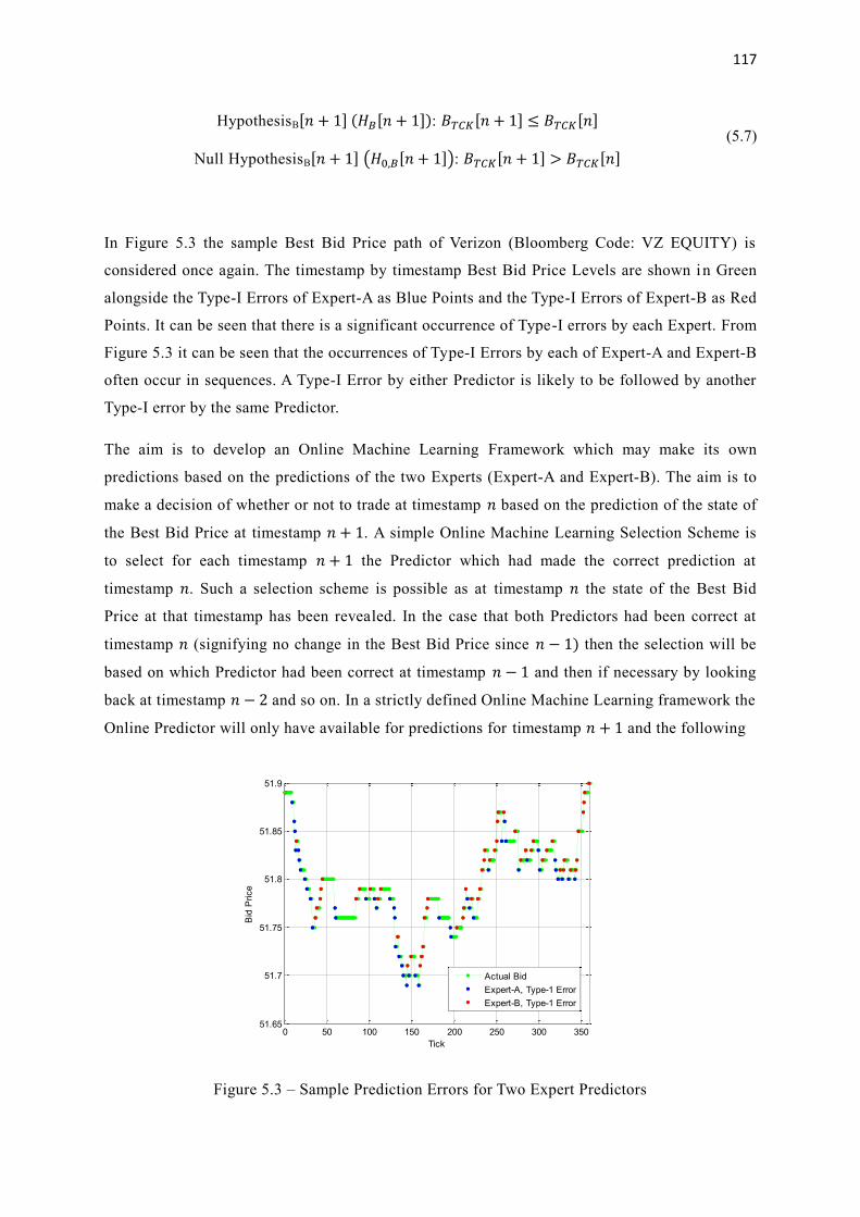
117

HypothesisB[𝑛 + 1] (𝐻𝐵[𝑛 + 1]): 𝐵𝑇𝐶𝐾[𝑛 + 1] ≤ 𝐵𝑇𝐶𝐾[𝑛]

Null HypothesisB[𝑛 + 1] (𝐻0,𝐵[𝑛 + 1]): 𝐵𝑇𝐶𝐾[𝑛 + 1] > 𝐵𝑇𝐶𝐾[𝑛]

(5.7)

In Figure 5.3 the sample Best Bid Price path of Verizon (Bloomberg Code: VZ EQUITY) is

considered once again. The timestamp by timestamp Best Bid Price Levels are shown in Green

alongside the Type-I Errors of Expert-A as Blue Points and the Type-I Errors of Expert-B as Red

Points. It can be seen that there is a significant occurrence of Type-I errors by each Expert. From

Figure 5.3 it can be seen that the occurrences of Type-I Errors by each of Expert-A and Expert-B

often occur in sequences. A Type-I Error by either Predictor is likely to be followed by another

Type-I error by the same Predictor.

The aim is to develop an Online Machine Learning Framework which may make its own

predictions based on the predictions of the two Experts (Expert-A and Expert-B). The aim is to

make a decision of whether or not to trade at timestamp 𝑛 based on the prediction of the state of

the Best Bid Price at timestamp 𝑛 + 1. A simple Online Machine Learning Selection Scheme is

to select for each timestamp 𝑛 + 1 the Predictor which had made the correct prediction at

timestamp 𝑛. Such a selection scheme is possible as at timestamp 𝑛 the state of the Best Bid

Price at that timestamp has been revealed. In the case that both Predictors had been correct at

timestamp 𝑛 (signifying no change in the Best Bid Price since 𝑛 − 1) then the selection will be

based on which Predictor had been correct at timestamp 𝑛 − 1 and then if necessary by looking

back at timestamp 𝑛 − 2 and so on. In a strictly defined Online Machine Learning framework the

Online Predictor will only have available for predictions for timestamp 𝑛 + 1 and the following

Figure 5.3 – Sample Prediction Errors for Two Expert Predictors

0 50 100 150 200 250 300 35051.65

51.7

51.75

51.8

51.85

51.9

Tick

Bid

Price

Actual Bid

Expert-A, Type-1 Error

Expert-B, Type-1 Error

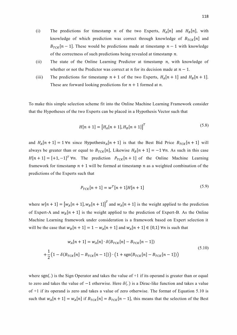
118

(i) The predictions for timestamp 𝑛 of the two Experts, 𝐻𝐴[𝑛] and 𝐻𝐵[𝑛], with

knowledge of which prediction was correct through knowledge of 𝐵𝑇𝐶𝐾[𝑛] and

𝐵𝑇𝐶𝐾[𝑛 − 1]. These would be predictions made at timestamp 𝑛 − 1 with knowledge

of the correctness of such predictions being revealed at timestamp 𝑛.

(ii) The state of the Online Learning Predictor at timestamp 𝑛, with knowledge of

whether or not the Predictor was correct at 𝑛 for its decision made at 𝑛 − 1.

(iii) The predictions for timestamp 𝑛 + 1 of the two Experts, 𝐻𝐴[𝑛 + 1] and 𝐻𝐵[𝑛 + 1].

These are forward looking predictions for 𝑛 + 1 formed at 𝑛.

To make this simple selection scheme fit into the Online Machine Learning Framework consider

that the Hypotheses of the two Experts can be placed in a Hypothesis Vector such that

𝐻[𝑛 + 1] = [𝐻𝐴[𝑛 + 1], 𝐻𝐵[𝑛 + 1]]𝑇 (5.8)

and 𝐻𝐴[𝑛 + 1] = 1 ∀𝑛 since Hypothesis𝐴[𝑛 + 1] is that the Best Bid Price 𝐵𝑇𝐶𝐾[𝑛 + 1] will

always be greater than or equal to 𝐵𝑇𝐶𝐾[𝑛], Likewise 𝐻𝐵[𝑛 + 1] = −1 ∀𝑛. As such in this case

𝐻[𝑛 + 1] = [+1,−1]𝑇 ∀𝑛. The prediction 𝑃𝑇𝐶𝐾[𝑛 + 1] of the Online Machine Learning

framework for timestamp 𝑛 + 1 will be formed at timestamp 𝑛 as a weighted combination of the

predictions of the Experts such that

𝑃𝑇𝐶𝐾[𝑛 + 1] = 𝑤𝑇[𝑛 + 1]𝐻[𝑛 + 1] (5.9)

where 𝑤[𝑛 + 1] = [𝑤𝐴[𝑛 + 1], 𝑤𝐵[𝑛 + 1]]𝑇

and 𝑤𝐴[𝑛 + 1] is the weight applied to the prediction

of Expert-A and 𝑤𝐵[𝑛 + 1] is the weight applied to the prediction of Expert-B. As the Online

Machine Learning framework under consideration is a framework based on Expert selection it

will be the case that 𝑤𝐵[𝑛 + 1] = 1 − 𝑤𝐴[𝑛 + 1] and 𝑤𝐴[𝑛 + 1] ∈ {0,1} ∀𝑛 is such that

𝑤𝐴[𝑛 + 1] = 𝑤𝐴[𝑛] ∙ 𝛿(𝐵𝑇𝐶𝐾[𝑛] − 𝐵𝑇𝐶𝐾[𝑛 − 1])

+1

2(1 − 𝛿(𝐵𝑇𝐶𝐾[𝑛] − 𝐵𝑇𝐶𝐾[𝑛 − 1])) ∙ (1 + sgn(𝐵𝑇𝐶𝐾[𝑛] − 𝐵𝑇𝐶𝐾[𝑛 − 1]))

(5.10)


to zero and takes the value of −1 otherwise. Here 𝛿(. ) is a Dirac-like function and takes a value

of +1 if its operand is zero and takes a value of zero otherwise. The format of Equation 5.10 is

such that 𝑤𝐴[𝑛 + 1] = 𝑤𝐴[𝑛] if 𝐵𝑇𝐶𝐾[𝑛] = 𝐵𝑇𝐶𝐾[𝑛 − 1], this means that the selection of the Best

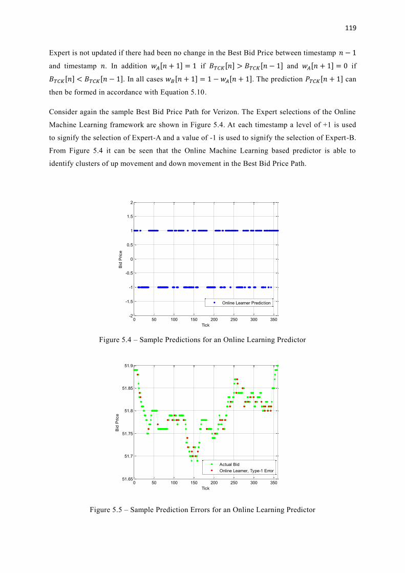
119

Expert is not updated if there had been no change in the Best Bid Price between timestamp 𝑛 − 1

and timestamp 𝑛. In addition 𝑤𝐴[𝑛 + 1] = 1 if 𝐵𝑇𝐶𝐾[𝑛] > 𝐵𝑇𝐶𝐾[𝑛 − 1] and 𝑤𝐴[𝑛 + 1] = 0 if

𝐵𝑇𝐶𝐾[𝑛] < 𝐵𝑇𝐶𝐾[𝑛 − 1]. In all cases 𝑤𝐵[𝑛 + 1] = 1 − 𝑤𝐴[𝑛 + 1]. The prediction 𝑃𝑇𝐶𝐾[𝑛 + 1] can

then be formed in accordance with Equation 5.10.

Consider again the sample Best Bid Price Path for Verizon. The Expert selections of the Online

Machine Learning framework are shown in Figure 5.4. At each timestamp a level of +1 is used

to signify the selection of Expert-A and a value of -1 is used to signify the selection of Expert-B.

From Figure 5.4 it can be seen that the Online Machine Learning based predictor is able to

identify clusters of up movement and down movement in the Best Bid Price Path.

Figure 5.4 – Sample Predictions for an Online Learning Predictor

Figure 5.5 – Sample Prediction Errors for an Online Learning Predictor

0 50 100 150 200 250 300 350-2

-1.5

-1

-0.5

0

0.5

1

1.5

2

Tick

Bid

Price

Online Learner Prediction

0 50 100 150 200 250 300 35051.65

51.7

51.75

51.8

51.85

51.9

Tick

Bid

Price

Actual Bid

Online Learner, Type-1 Error

120

The occurrence of Type-I Errors by the Online Learning Predictor is shown in Figure 5.5. From

the Figure it can be seen that there is a reduction in the number of Type-I Errors compared to

that made individually by Expert-A and Expert-B. The current method effectively looks to

follow a short term trend based on the direction of the Best Bid Price over the one timestamp

interval between timestamp 𝑛 − 1 and timestamp 𝑛. The performance measure that is based on

the occurrence of Type-I Errors is effectively a measure of the probability of an incorrect

prediction in the direction of the Best Bid Price over an interval of one timestamp. In practice

however it is the probability of a trading profit that is important.

Thus far a method of following the short term trend based on the direction of the Best Bid Price

over the one timestamp interval between timestamp 𝑛 − 1 and timestamp 𝑛 has been considered.

At each timestamp 𝑛 a potential sell trade can be placed at the then Best Bid Price 𝐵𝑇𝐶𝐾[𝑛] or a

decision can be made to wait for some number 𝑗 ≥ 0 of timestamps. The profit or loss of the

final trading decision that begins at timestamp 𝑛 can then be expressed as

𝑄𝑇𝐶𝐾[𝑛] = 𝐵𝑇𝐶𝐾[𝑛] − 𝐵𝑇𝐶𝐾[𝑛 + 𝑗] (5.11)

The sample Best Bid Price path of Figure 5.5 is again considered in Figure 5.6, the timestamps

at which a profitable sell trade is eventually determined are shown as Blue points and the

timestamps at which a loss making sell trade is eventually determined are shown as Red points.

From Figure 5.6 it can be seen that the Online Machine Learning Framework that has been

developed so far is unable to find many profitable trading opportunities over the sample Best

Bid Price path and a lot of losses are incurred.

Figure 5.6 – Profitable and Loss Making Trades for an Online Learning Predictor

0 50 100 150 200 250 300 35051.65

51.7

51.75

51.8

51.85

51.9

Tick

Bid

Price

Actual Bid

Profitable

Loss Making

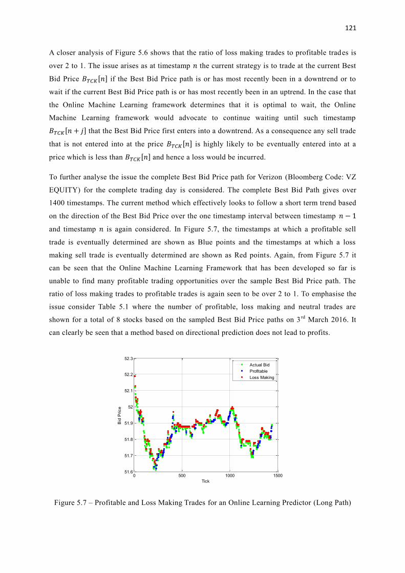
121

A closer analysis of Figure 5.6 shows that the ratio of loss making trades to profitable trades is

over 2 to 1. The issue arises as at timestamp 𝑛 the current strategy is to trade at the current Best

Bid Price 𝐵𝑇𝐶𝐾[𝑛] if the Best Bid Price path is or has most recently been in a downtrend or to

wait if the current Best Bid Price path is or has most recently been in an uptrend. In the case that

the Online Machine Learning framework determines that it is optimal to wait, the Online

Machine Learning framework would advocate to continue waiting until such timestamp

𝐵𝑇𝐶𝐾[𝑛 + 𝑗] that the Best Bid Price first enters into a downtrend. As a consequence any sell trade

that is not entered into at the price 𝐵𝑇𝐶𝐾[𝑛] is highly likely to be eventually entered into at a

price which is less than 𝐵𝑇𝐶𝐾[𝑛] and hence a loss would be incurred.

To further analyse the issue the complete Best Bid Price path for Verizon (Bloomberg Code: VZ

EQUITY) for the complete trading day is considered. The complete Best Bid Path gives over

1400 timestamps. The current method which effectively looks to follow a short term trend based

on the direction of the Best Bid Price over the one timestamp interval between timestamp 𝑛 − 1

and timestamp 𝑛 is again considered. In Figure 5.7, the timestamps at which a profitable sell

trade is eventually determined are shown as Blue points and the timestamps at which a loss

making sell trade is eventually determined are shown as Red points. Again, from Figure 5.7 it

can be seen that the Online Machine Learning Framework that has been developed so far is

unable to find many profitable trading opportunities over the sample Best Bid Price path. The

ratio of loss making trades to profitable trades is again seen to be over 2 to 1. To emphasise the

issue consider Table 5.1 where the number of profitable, loss making and neutral trades are

shown for a total of 8 stocks based on the sampled Best Bid Price paths on 3rd

March 2016. It

can clearly be seen that a method based on directional prediction does not lead to profits.

Figure 5.7 – Profitable and Loss Making Trades for an Online Learning Predictor (Long Path)

0 500 1000 150051.6

51.7

51.8

51.9

52

52.1

52.2

52.3

Tick

Bid

Price

Actual Bid

Profitable

Loss Making

122

Stock Name Ticker Loss Making Neutral Profitable

1 Verizon VZ 497 702 240

2 Caterpillar CAT 408 732 299

3 Chevron CVX 430 760 249

4 Coca Cola KO 476 741 222

5 Dupont DD 449 747 243

6 Exxon XOM 411 796 232

7 IBM IBM 458 752 229

8 McDonalds MCD 474 752 213

Average 450.4 747.8 240.9

Table 5.1 - Application of an Online Learning Framework to Sample Stocks

To move forward an alternative Performance Measure (PER) to the number of Type-I Errors in the

directional prediction at the next time stamp is needed. The focus needs to be directly upon

determining when it would and would not be profitable to trade. Consider again the case that a

sell trade can be entered into at timestamp 𝑛 by selling at the Best Bid Price 𝐵𝑇𝐶𝐾[𝑛]; the Online

Machine Learning Framework should again decide to either trade at timestamp 𝑛 or to wait until

timestamp 𝑛 + 1 and re-evaluate. The decision to wait should however be on the basis that a

more profitable opportunity may in expectation be found within this decide or wait framework at

timestamp 𝑛 + 1 and not on a belief that the Best Bid Price will be higher at timestamp 𝑛 + 1.

To move forward consider that the Online Machine Learning Framework developed above itself

becomes an Expert which shall be termed Expert-C. Expert-C makes a directional prediction

based on the direction of the Best Bid Price over the one timestamp interval from timestamp

𝑛 − 1 to timestamp 𝑛. The results in Table 5.1 would suggest that a simple strategy would be to

counter the decisions of Expert C and to trade at the Best Bid Price 𝐵𝑇𝐶𝐾[𝑛] when Expert-C

makes a decision to wait and to wait when Expert C suggests to trade at 𝐵𝑇𝐶𝐾[𝑛]. The results of

such a strategy are shown in Table 5.2.


1 Verizon VZ 198 879 362



4 Coca Cola KO 178 896 365

5 Dupont DD 170 811 458

6 Exxon XOM 246 779 414

7 IBM IBM 223 749 467


Average 203.0 812.1 423.9

Table 5.2 - Application of Countering an Online Learning Framework to Sample Stocks

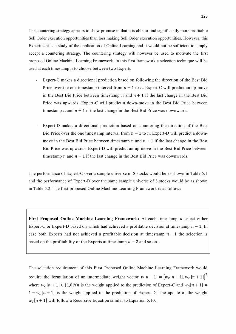
123

The countering strategy appears to show promise in that it is able to find significantly more profitable

Sell Order execution opportunities than loss making Sell Order execution opportunities. However, this

Experiment is a study of the application of Online Learning and it would not be sufficient to simply

accept a countering strategy. The countering strategy will however be used to motivate the first

proposed Online Machine Learning Framework. In this first framework a selection technique will be

used at each timestamp 𝑛 to choose between two Experts

- Expert-C makes a directional prediction based on following the direction of the Best Bid

Price over the one timestamp interval from 𝑛 − 1 to 𝑛. Expert-C will predict an up-move

in the Best Bid Price between timestamp 𝑛 and 𝑛 + 1 if the last change in the Best Bid

Price was upwards. Expert-C will predict a down-move in the Best Bid Price between

timestamp 𝑛 and 𝑛 + 1 if the last change in the Best Bid Price was downwards.

- Expert-D makes a directional prediction based on countering the direction of the Best

Bid Price over the one timestamp interval from 𝑛 − 1 to 𝑛. Expert-D will predict a down-

move in the Best Bid Price between timestamp 𝑛 and 𝑛 + 1 if the last change in the Best

Bid Price was upwards. Expert-D will predict an up-move in the Best Bid Price between


The performance of Expert-C over a sample universe of 8 stocks would be as shown in Table 5.1

and the performance of Expert-D over the same sample universe of 8 stocks would be as shown

in Table 5.2. The first proposed Online Machine Learning Framework is as follows

First Proposed Online Machine Learning Framework: At each timestamp 𝑛 select either

Expert-C or Expert-D based on which had achieved a profitable decision at timestamp 𝑛 − 1. In

case both Experts had not achieved a profitable decision at timestamp 𝑛 − 1 the selection is

based on the profitability of the Experts at timestamp 𝑛 − 2 and so on.

The selection requirement of this First Proposed Online Machine Learning Framework would

require the formulation of an intermediate weight vector 𝑤[𝑛 + 1] = [𝑤𝐶[𝑛 + 1], 𝑤𝐷[𝑛 + 1]]𝑇

where 𝑤𝐶[𝑛 + 1] ∈ {1,0}∀𝑛 is the weight applied to the prediction of Expert-C and 𝑤𝐷[𝑛 + 1] =

1 − 𝑤𝐶[𝑛 + 1] is the weight applied to the prediction of Expert-D. The update of the weight

𝑤𝐶[𝑛 + 1] will follow a Recursive Equation similar to Equation 5.10.

124

For clarity if a decision is made to follow Expert-C at some timestamp 𝑛 − 1 the profit or loss of

that decision will be determined according to Equation 5.11 and as such the profit or loss will

not be determined until some number of timestamps 𝑗 ≥ 0 following the decision at timestamp

𝑛 − 1. If it is the case that 𝑗 > 1 then the profit or loss of the decision of Expert-C will not be

known at timestamp 𝑛 and therefore cannot be used to influence the selection decision of an

Online Learning Predictor at timestamp 𝑛. The same reasoning will apply to Expert-D.

The sample Best Bid Price path of Verizon (Bloomberg Code: VZ EQUITY) is again considered.

The Expert selection decisions of this First Proposed Online Learning Predictor are shown in

Figure 5.8. The Profit or Loss of the decisions of the Predictor are as shown in Figure 5.9.

Figure 5.8 – Expert Selection Decisions of the First Proposed Online Learning Predictor

Figure 5.9 – Profit or Loss of the Decisions of the First Proposed Online Learning Predictor

0 50 100 150 200 250 300 35051.65

51.7

51.75

51.8

51.85

51.9

Tick

Bid

Price

Actual Bid

Expert-C

Expert-D

0 50 100 150 200 250 300 35051.65

51.7

51.75

51.8

51.85

51.9

Tick

Bid

Price

Actual Bid

Profitable

Loss Making

125


1 Verizon VZ 170 982 286



4 Coca Cola KO 111 1022 305

5 Dupont DD 172 888 378

6 Exxon XOM 251 849 338

7 IBM IBM 242 825 371


Average 193.3 896.1 348.6

Table 5.3 - Application of a First Proposed Online Learning Framework to Sample Stocks

From Figure 5.8 it can be seen that Expert-D is the most commonly chosen Expert; this is not

surprising as the results of Table 5.2 would suggest that Expert-D is the most profitable Expert.

Further analysis is shown in Table 5.3 where the results of Table 5.2 are reproduced to show the

performance of the First Proposed Online Machine Learning Framework across a test universe of

8 stocks. From Table 5.3 it can be seen that this First Proposed Online Machine Learning

Framework is able to find more profitable trading opportunities than loss making opportunities

and as such by a simple measure of profitability the framework does appear to work.

This First Proposed Online Machine Learning Framework is based on the Follow the Leader

technique where the Leader is followed based on performance over a one timestamp interval. To

extend the method the Follow the Leader method may be considered again where the Leader is

determined to be that expert who has generated the most profitable trades over some longer

interval of 𝐿 timestamps.

Second Proposed Online Machine Learning Framework: At each timestamp 𝑛 select either

Expert-C or Expert-D based on which had achieved the most profitable decisions over the

preceding 𝐿 timestamps. In case both Experts had achieved the same profitability at timestamp 𝑛

the decision will be based on profitability at timestamp 𝑛 − 1, then timestamp 𝑛 − 2 and so on.

The First Proposed Online Machine Learning Framework is then a special case of the Second

Proposed Online Machine Learning Framework with 𝐿 = 1. The performance results for this

Second Proposed Online Machine Learning Framework are shown in Tables 5.4 to 5.6 on the

next page for increasing values of 𝐿.

126

Stock Name Ticker Losing Neutral Profitable %Profitable %Expert D

1 Verizon VZ 170 982 286 62.7% 88.0%

2 Caterpillar CAT 202 881 355 63.7% 84.0%

3 Chevron CVX 213 821 404 65.5% 84.6%

4 Coca Cola KO 111 1022 305 73.3% 85.7%

5 Dupont DD 172 888 378 68.7% 83.7%

6 Exxon XOM 251 849 338 57.4% 83.5%

7 IBM IBM 242 825 371 60.5% 86.2%

8 McDonalds MCD 185 901 352 65.5% 83.2%

Average 193.3 896.1 348.6 64.7% 84.9%

Table 5.4 - Application of a Second Proposed Online Learning Framework 𝐿 = 1


1 Verizon VZ 215 923 281 56.7% 78.1%

2 Caterpillar CAT 250 756 413 62.3% 70.5%

3 Chevron CVX 252 729 438 63.5% 77.5%

4 Coca Cola KO 184 926 309 62.7% 77.0%

5 Dupont DD 212 831 376 63.9% 73.3%

6 Exxon XOM 263 813 343 56.6% 74.2%

7 IBM IBM 283 757 379 57.3% 76.7%

8 McDonalds MCD 272 818 329 54.7% 72.0%

Average 241.4 819.1 358.5 59.7% 74.9%



1 Verizon VZ 247 717 275 52.7% 67.5%

2 Caterpillar CAT 205 658 376 64.7% 78.8%

3 Chevron CVX 199 643 397 66.6% 89.3%

4 Coca Cola KO 160 873 206 56.3% 76.8%

5 Dupont DD 165 695 379 69.7% 92.9%

6 Exxon XOM 216 690 333 60.7% 85.5%

7 IBM IBM 200 652 387 65.9% 87.3%

8 McDonalds MCD 179 712 348 66.0% 99.9%

Average 196.4 705.0 337.6 62.8% 84.7%


From Table 5.4 it can indeed be seen that the performance in the case that 𝐿 = 1 is identical to

that from the First Proposed Online Machine Learning Framework. An analysis of Tables 5.4 to

5.6 would show that as 𝐿 is increased there is an initial deterioration in performance as signalled

by a decrease in the percentage of profitable trades in moving from 𝐿 = 1 to 𝐿 = 20. However

127

this initial deterioration in performance does eventually give over to increasing performance

once again as 𝐿 is further increased from 𝐿 = 20 to 𝐿 = 200. At 𝐿 = 1 there is an initial strong

preference to choose Expert-D, this preference decays away as 𝐿 is increased towards 𝐿 = 20,

but the preference is again recovered as 𝐿 moves towards 𝐿 = 200.

The results of Tables 5.4 to 5.6 do suggest that the optimal value of 𝐿 is 𝐿 = 1. This is an

interesting and highly meaningful result. The result would suggest that most information

regarding the state of the Market Order Book in the near future is captured in the most recent

historical behaviour of the Market Order Book. It is the near term behaviour that is most

important. This conclusion would add further support to the premise that models of the dynamics

of the Double Auction Based Limit Order Book which require calibration over long term statistics

may not be well suited to determine the optimal time to place Market Orders.

The results of Table 5.4 to 5.6 also shed light on the behaviour of Market Order Book in a short time

interval. The results suggest that the optimal strategy would be to counter the direction of the Market

Order Book over a short interval of time. This would suggest that that over such a short interval of

time there might exist a pattern of Market Order Book oscillation where the Best Bid Price is toggling

up and down. This would be the case, for example, if the Market Order Book were static but there

were interspersed Market Orders to Buy and Market Orders to Sell which were hitting the Order

Book. Such Buy and Sell orders would cause the Best Bid Price to toggle up and toggle down. The

Second Online Machine Learning Framework with 𝐿 = 1 would then be capturing the existence of

such Buy and Sell orders and would be prosing a strategy to trade around such orders.

The Second Proposed Online Machine Learning Framework is based on the Method of Follow

the Leader over various intervals of 𝐿 timestamps. In this case the performance is based on the

number of correct predictions where correct is defined to be profitable. In this framework there

is no specific penalisation of incorrect predictions. An alternative Online Machine Learning

Framework would be that based upon the Weighted Majority Algorithm which has been shown

in Equation 2.9. In the standard Weighted Majority Algorithm a Weight Vector is specified as

𝑤[𝑛 + 1] = [𝑤1[𝑛 + 1], 𝑤2[𝑛 + 1], … ,𝑤𝑑[𝑛 + 1]]𝑇

(5.12)

where there are 𝑑 Experts in total and 𝑤𝑎[𝑛 + 1] is the weight assigned at timestamp 𝑛 to the

forward looking prediction for timestamp 𝑛 + 1 of Expert 𝑎. At timestamp 0 the Weight Vector

𝑤[0] is initialised as a vector of ones. At each successive timestamp 𝑤𝑎[𝑛 + 1] = 𝑤𝑎[𝑛] if

Expert-a had made a correct prediction at timestamp 𝑛 and 𝑤𝑎[𝑛 + 1] = 𝛽𝑤𝑎[𝑛] with 𝛽 < 1 in

the case that Expert-a had made an incorrect prediction at timestamp 𝑛. The effect is to penalise

each expert by some Factor 𝛽 in the case that it makes an incorrect prediction.

128

Here an extension of the Weighted Majority Algorithm is considered. At each successive

timestamp 𝑤𝑎[𝑛 + 1] = 𝛽𝑤𝑎[𝑛] if Expert-a had made a correct prediction at timestamp 𝑛 and

𝑤𝑎[𝑛 + 1] = (1

𝛽)𝑤𝑎[𝑛] with 𝛽 > 1 in the case that Expert-a had made an incorrect prediction at

timestamp 𝑛. The effect is to reward each expert by some Factor 𝛽 in the case that it makes a

correct prediction and to penalise each expert by some Factor 1/𝛽 in the case that it makes an

incorrect prediction. The Extended Weighted Majority Algorithm is initialised such that the

Weight Vector 𝑤[0] is initialised as a vector of ones. Once again Expert-C and Expert-D as

defined above are considered in a Third Proposed Online Machine Learning Framework

Third Proposed Online Machine Learning Framework: At each timestamp 𝑛 adjust the

forward looking weights 𝑤𝐶[𝑛] and 𝑤𝐷[𝑛] of Expert-C and Expert-D respectively based on

whether or not they had achieved a profitable trading decision for timestamp 𝑛 (such decision

being made prior to timestamp 𝑛). In the case of Expert-C 𝑤𝐶[𝑛 + 1] = 𝛽𝑤𝐶[𝑛] if Expert-C had

made a profitable decision, 𝑤𝐶[𝑛 + 1] = (1

𝛽)𝑤𝐶[𝑛] if Expert-C had made a loss making decision

and 𝑤𝐶[𝑛 + 1] = 𝑤𝐶[𝑛] if the decision had been profit neutral. The update logic applied to

Expert-D is the same as that applied to Expert-C.

The Factor 𝛽 can be used to control the rate at which a bad performing Expert is penalised. For

example in the case that 𝛽 = 1.10 an incorrect prediction would reduce the weight of an Expert

by around 9%, two successive incorrect predictions would reduce the weight by around 17% and

three successive incorrect predictions would reduce the weight by around 25%. In the case that

𝛽 = 1.50 an incorrect prediction would reduce the weight of an Expert by around 33%, two

successive incorrect predictions would reduce the weight by around 56% and three successive

incorrect predictions would reduce the weight by over 70%. Unlike in the case of the Second

Proposed Online Machine Learning Framework there is no value of 𝛽 which would reduce this

Third Proposed Online Machine Learning Framework to mimic the behaviour of the First

Proposed Online Machine Learning Framework.

The performance results for this Third Proposed Online Machine Learning Framework are

shown in Tables 5.7 to 5.9 for increasing values of 𝛽. The results shed further light on the

behaviour of the Best Bid Price in the Market Order Book and how to optimally trade the Market

Order Book when it comes to placing Market Orders.

129


1 Verizon VZ 199 871 360 64.4% 99.9%

2 Caterpillar CAT 272 724 434 61.5% 62.9%

3 Chevron CVX 204 759 467 69.6% 100.0%

4 Coca Cola KO 178 888 364 67.2% 100.0%

5 Dupont DD 173 809 448 72.1% 89.6%

6 Exxon XOM 249 768 413 62.4% 99.7%

7 IBM IBM 234 734 462 66.4% 98.9%

8 McDonalds MCD 212 808 410 65.9% 100.0%

Average 215.1 795.1 419.8 66.2% 93.9%

Table 5.7 - Application of a Third Proposed Online Learning Framework 𝛽 = 1.10


1 Verizon VZ 194 868 358 64.9% 100.0%

2 Caterpillar CAT 271 722 427 61.2% 63.3%

3 Chevron CVX 202 754 464 69.7% 100.0%

4 Coca Cola KO 178 883 359 66.9% 100.0%

5 Dupont DD 170 808 442 72.2% 90.2%

6 Exxon XOM 244 765 411 62.7% 100.0%

7 IBM IBM 227 731 462 67.1% 99.4%

8 McDonalds MCD 211 803 406 65.8% 100.0%

Average 212.1 791.8 416.1 66.3% 94.1%



1 Verizon VZ 186 854 350 65.3% 100.0%

2 Caterpillar CAT 264 718 408 60.7% 65.0%

3 Chevron CVX 197 741 452 69.6% 100.0%

4 Coca Cola KO 165 873 352 68.1% 100.0%

5 Dupont DD 163 785 442 73.1% 92.2%

6 Exxon XOM 233 756 401 63.2% 100.0%

7 IBM IBM 221 711 458 67.5% 100.0%

8 McDonalds MCD 200 793 397 66.5% 100.0%

Average 203.6 778.9 407.5 66.8% 94.6%


The results of Table 5.7 to 5.9 suggest that the performance of the Third Proposed Online

Machine Learning Framework is similar for different values of the Factor 𝛽. It can also be seen

that the Third Proposed Online Machine Learning Framework is able to outperform the Second

Proposed Online Machine Learning Framework over the sample test set of 8 stocks. From Table

130

5.7 to 5.9 it does appear that there is a general preference of Expert-D as it can be seen that for

many stocks the proportion of time that Expert-D is chosen is close to or equal to 100%.

However one clear exception is the second Stock (Caterpillar, Bloomberg Code CAT US

EQUITY) where it appears that Expert-C is quote often chosen as the preferred Expert. This also

sheds some light on the behaviour of the Best Bid Price in the Market Order Book.

Where there is a strong preference for Expert-D the optimal strategy would be to counter the direction

of the Market Order Book over a short interval of time. This would again suggest that that over such a

short interval of time there exists a pattern of Market Order Book oscillation where the Best Bid Price

is toggling up and down and it would again be the case that the Third Proposed Online Machine

Learning Framework is suggesting a strategy to profitably trade around this oscillating order book. In

the case of Caterpillar it appears that there are also strong directional trends that can be identified in

the order book and as such there is an occasional preference for Expert-C. It is clear that the Third

Proposed Online Machine Learning Framework had been more successful than the Second Proposed

Online Machine Learning Framework in detecting an Order Book that is either oscillating or showing

trends and this is illustrated by the fact that the Third Framework is more profitable than the Second.

In the next section Test Results over a wider universe of stocks are used to analyse the proposed

Online Machine Learning Frameworks.

5.4 Testing the Proposed Methods

In the previous section the development of three Online Machine Learning Frameworks for the

determination of the optimal timing at which to place Market Orders into the Double Auction

Based Limit Order Book was presented. These frameworks were based on Adversarial Models of

Online Machine Learning. The frameworks considered just two underlying Experts:









131



Of the three Online Machine Learning Frameworks that were presented it was shown that the First

Framework is simply a special case of the Second Framework. The analysis in this section therefore

focusses on just two of the three frameworks

- Framework-2: Based on the Follow the Leader Technique. At each timestamp 𝑛 select either

Expert-C or Expert-D based on which had achieved the most profitable decisions over the

preceding 𝐿 timestamps. In case both Experts had achieved the same profitability at

timestamp 𝑛 the decision will be based on profitability at timestamp 𝑛 − 1, then timestamp

𝑛 − 2 and so on.

- Framework-3: Based on an Extended Weighted Majority Algorithm. At each timestamp 𝑛

adjust the forward looking weights 𝑤𝐶[𝑛] and 𝑤𝐷[𝑛] of Expert-C and Expert-D

respectively based on whether or not they had achieved a profitable trading decision for

timestamp 𝑛 (such decision being made prior to timestamp 𝑛). In the case of Expert-C

𝑤𝐶[𝑛 + 1] = 𝛽𝑤𝐶[𝑛] if Expert-C had made a profitable decision, 𝑤𝐶[𝑛 + 1] = (1

𝛽)𝑤𝐶[𝑛]

if Expert-C had made a loss making decision and 𝑤𝐶[𝑛 + 1] = 𝑤𝐶[𝑛] if the decision had

been profit neutral. The update logic applied to Expert-D is the same as that applied to

Expert-C.

An extended universe of 32 stocks is considered for the trading date of 29th April 2016. The

performance of Framework-2 is illustrated in Figure 5.10 and Figure 5.11. In Figure 5.10 the average

Percentage of Profitable Trades is shown for various values of the Window Length 𝐿 across the

universe of 32 stocks. For each stock the performance is taken over 1440 timestamps representing the

sampled Best Bid Price of the Market Order Book at 15 second intervals over the trading session of 6

hours. In Figure 5.11 the average Percentage of Timestamps for Which Expert-D is Chosen is shown

for various values of the Window Length 𝐿 across the universe of 32 stocks.

From Figure 5.10 it can again be seen that there is an initial deterioration of performance as the

Window Length 𝐿 is increased and this is later followed by an increase in performance as the

Window Length 𝐿 is further increased. From Figure 5.10 it can be seen that there is an initial

preference for Expert-D which gives way to a preference for Expert-C as the Window Length 𝐿

is increased, further increases in the Window Length 𝐿 then give over again to an increased

preference for Expert-D.

132

Figure 5.10 - Average Percentage of Profitable Trades for the Window Length 𝐿

Figure 5.11 - Average Percentage for Which Expert-D is Chosen for the Window Length 𝐿

From Figure 5.10 and Figure 5.11 it can again be determined that much of the information

regarding the state of the Market Order Book in the near future is captured in the most recent

historical behaviour of the Market Order Book, this is concluded because the performance for

𝐿 = 1 is close to the maximal performance that can be achieved for various values of 𝐿. At the

same time the absolute maximal performance is achieved for a high value of 𝐿 and performance

is seen to be increasing with Window Length 𝐿 increasing further. The later observation coupled

with an increased preference for Expert-D would suggest that over the longer term the Best Bid

Price of the Market Order Book may show an oscillatory behaviour ticking up and down.

0 20 40 60 80 100 120 140 160 180 200

0.58

0.59

0.6

0.61

0.62

0.63

0.64

Window Length, L

% P

rofita

ble

% Profitable, Sell Side

0 20 40 60 80 100 120 140 160 180 2000.72

0.74

0.76

0.78

0.8

0.82

0.84

0.86

0.88

0.9

0.92

Window Length, L

% E

xpert

-D

% Expert-D, Sell Side

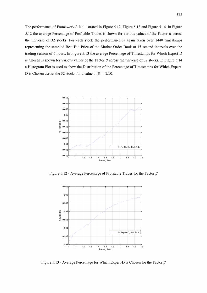
133

The performance of Framework-3 is illustrated in Figure 5.12, Figure 5.13 and Figure 5.14. In Figure

5.12 the average Percentage of Profitable Trades is shown for various values of the Factor 𝛽 across

the universe of 32 stocks. For each stock the performance is again taken over 1440 timestamps

representing the sampled Best Bid Price of the Market Order Book at 15 second intervals over the

trading session of 6 hours. In Figure 5.13 the average Percentage of Timestamps for Which Expert-D

is Chosen is shown for various values of the Factor 𝛽 across the universe of 32 stocks. In Figure 5.14

a Histogram Plot is used to show the Distribution of the Percentage of Timestamps for Which Expert-

D is Chosen across the 32 stocks for a value of 𝛽 = 1.10.

Figure 5.12 - Average Percentage of Profitable Trades for the Factor 𝛽

Figure 5.13 - Average Percentage for Which Expert-D is Chosen for the Factor 𝛽

1 1.1 1.2 1.3 1.4 1.5 1.6 1.7 1.8 1.9 20.636

0.638

0.64

0.642

0.644

0.646

0.648

0.65

0.652

0.654

0.656

Factor, Beta

% P

rofita

ble

% Profitable, Sell Side

1 1.1 1.2 1.3 1.4 1.5 1.6 1.7 1.8 1.9 20.93

0.935

0.94

0.945

0.95

0.955

0.96

0.965

Factor, Beta

% E

xpert

-D

% Expert-D, Sell Side

134

Figure 5.14 - Distribution of the Percentage of Time for Which Expert-D is Chosen 𝛽 = 1.10

From Figure 5.12 it can be seen that there is an increase in performance as the Factor 𝛽 is increased

and from Figure 5.13 it can be seen that there is an increased preference for Expert-D as the

Factor 𝛽 is increased. An analysis of the results of these figures in isolation would suggest that

that over the longer term the Best Bid Price of the Market Order Book may show an oscillatory

behaviour ticking up and down. To put this effect into detail , where there is a strong preference for

Expert-D the optimal strategy would be to counter the direction of the Market Order Book over a

short interval of time. This would then suggest that that over such a short interval of time there exists

a pattern of Market Order Book oscillation where the Best Bid Price is toggling up and down and it

would be the case that Framework-C is suggesting a strategy to profitably trade around this oscillating

order book. The conclusion is interesting and sheds some light on the behaviour of the Best Bid Price

of the Market Order Book.

This conclusion has however been reached by a consideration of the average behaviour of the stocks

over a universe of 32 stocks. In Figure 5.14 the stock by stock behaviour can be seen for an example

Factor of 𝛽 = 1.10. From Figure 5.14 it can be seen that although there may be a preference for

Expert-D on average, there is one stock for which there is a clear preference for Expert-C and

other stocks for which Expert-D is preferred at most timestamps but Expert-C is preferred at

other timestamps. The conclusion then is that at most time the Best Bid Price may exhibit some

form of oscillatory behaviour but at other times there will be clearly identifiable trends in the

Best Bid Price of the Market Order Book. A comparison of the results in Figure 5.12 and Figure

5.10 would suggest the Framework-3 is able to achieve a greater degree of profitability than

Framework-2 and as such Framework-3 should be chosen as the preferred Framework.

0.4 0.5 0.6 0.7 0.8 0.9 10

2

4

6

8

10

12

14

16

18

20

% Expert-D

Num

ber

of

Sto

cks

135

5.5 Summary

In this Chapter the development of three Online Machine Learning Frameworks for the

determination of the optimal timing at which to place Market Orders into the Double Auction

Based Limit Order Book have been presented. These frameworks were based on Adversarial Models

of Online Learning and both techniques of Follow the Leader and The Weighted Majority

Algorithm have been considered. The techniques considered just two underlying Experts











The framework based on just two experts allowed a number of conclusions to be drawn about

the behaviour of the Best Bid Price in the Double Auction Based Limit Order Book. The first

conclusion was that much of the information regarding the state of the Market Order Book in the

near future is captured in the most recent historical behaviour of the Market Order Book. The

second conclusion was that for the average stock it would most often be optimal to follow

Expert-D and to bet against the recent short term trend of the Market Order Book, this would

suggest that over a short interval of time there exists a pattern of Market Order Book oscillation

where the Best Bid Price is toggling up and down and it would be the case that following Expert-D

would provide a profitable strategy to trade around the oscillating order book. The third conclusion

was that using a method based upon The Weighted Majority Algorithm it would be the case that

stocks can be identified for which Expert-C is the preferred expert for some significant amount

of time and as such there could be identified periods of directional trend for the Best Bid Price.

The methods developed in this Chapter would allow additional profitability to be achieved beyond

that from the novel methods which have been developed in Chapter 3 and Chapter 4. The methods

developed in this Chapter would allow easy integration with the methods of the previous Chapters.

136

Chapter 6

Assessment

In this Chapter an Assessment of each of the three experiments is presented. This Chapter aims to

summarise the key points of each experiment. The Assessment begins with an Introduction which is

followed by a presentation of the key points of each experiment in turn.

6.1 Introduction

In Chapter 1 it was stated that in the period from 2010 to 2015 the vast majority of US Stock Funds

based on Active Management had failed to beat the broad Market Indices and such underperformance

was also seen over previous years. The fact that ‘Beating the Index’ had proven tough, at least for the

average human analyst, had served as the starting motivation of this Thesis. The overall objective was

to show that a Machine could do better. An overview of a complete trading strategy was presented in

Figure 2.5 and the three building blocks of such a strategy were identified. These three building

blocks are Trend Detection, Portfolio Construction and finally Order Entry Timing. This Thesis aimed

to develop original methods to approach these three building blocks in a commercially practical

manor whilst making contributions to the Academic Literature. The Thesis aimed to create building

blocks that could be connected to form a complete trading strategy.

The first experiment focussed on finding short term trading opportunities at the level of an individual

single stock. A novel Neural Network based method for detecting trading opportunities based on

betting with or against a recent short term trend was presented. The approach taken was a departure

from the bulk of the literature where the focus has generally been on next day direction prediction.

The second experiment considered the issue of Portfolio Construction. A Graphical Model framework

for Portfolio Construction under conditions where trades are only held for short periods of time was

presented. The work is important as standard Portfolio Construction techniques are not well suited to

highly dynamic Portfolios. The third experiment considered the issue of Order Execution and how to

optimally time the entry of trading orders into the market. The experiment demonstrated how Online

Learning techniques could be used to determine more optimal timing for Market Order Entry. This

work is important as order timing for Trade Execution has not been widely studied in the literature.

The approach taken in developing the original techniques in this Thesis has been to avoid data mining.

The techniques aimed to build upon over a decades experience as a Quantitative Analyst and as a

Trader and to always stay grounded in economic rationality. In the sections that follow each of the

three experiments is assessed it turn. The key points of each experiment are summarised, the original

contributions are highlighted and the testing results are discussed.

137

6.2 Assessment Of A New Neural Network Method For Profitable Long Short

Equity Trading

The first building block of a Complete Trading Strategy was identified as Trading Opportunity or

Trend Detection. In the Introduction to this Thesis it was reasoned through a discussion of the

Efficient Markets Hypothesis that trading opportunities could be found through the detection of

Momentum Anomalies and Overreaction Anomalies in price series data. With this as motivation a

novel Neural Network based method for detecting such trading opportunities through a direct search

for Momentum and Overreaction Anomalies was then presented in Chapter 3.

In the Background Chapter of this Thesis an overview of the current state of the art of methods for

Trading Opportunity detection was presented. A number of methods for trading opportunity detection

which centred on Fundamental Analysis and Technical Analysis were presented and the limitations of

such methods in finding trading opportunities under changing market conditions were discussed.

These limitations provided the motivation for the consideration of Machine Learning Techniques. The

review of the current state of the art then proceeded to investigate current methods for the application

of Machine Learning towards trading opportunity detection. A number of methods based on Multiple

Discriminant Analysis (MDA), Neural Networks and Support Vector Machines (SVM) were

presented and common to these methods was the use of a number of Technical Analysis indicators,

such indicators being used without any economic rationale. The theme was commonly to throw a lot

of Technical Analysis data at a Machine Learning technology and to leave that technology to try and

discern patterns in the data, the results were unsurprisingly underwhelming. The use of Input Feature

Selection techniques, including those based on Wrapper Methods and Filter Methods, was also

considered. Although such methods do lead to effective data dimension reduction, these methods were

not shown to lead to a significant improvement in performance. The overall conclusion was that

current methods simply lack economic rationality and there is no reason why they should work.

In Chapter 3 a novel framework for Trading Opportunity (trend) Detection has been presented.

The stating point of the framework considered just a combination of two technical analysis

indicators and showed how these indicators could be used for the detection of Overreaction and

Momentum anomalies without the employment of any Machine Learning technology. The core

of the method was to accept that at most times the market for a particular stock would be

efficient and as such the focus should not be to predict next day direction but to attempt to find

anomalies. This laid down an economic rationale upon which to move forward. An initial

attempt was then made to apply Machine Learning to this starting framework and it was shown

over a small testing universe that little success could be achieved. A second attempt at the

application of a Neural Network which addressed a number of issues was then presented.

138

The second attempt introduced a classification scheme for detected trading opportunities that

allowed for the classification of Outliers, this is an important consideration that is typically

overlooked in the development of Neural Network based trading strategies as considered in the

Academic Literature. Without a scheme for the treatment of outliers a Neural Network method

may be prone to overfitting. A method of Heuristic Regularisation was also introduced to deal

with the fact that a typically available Training Set would not span the full Input Feature Space;

the regularisation method termed Zero Appending introduced regularly spaced artefacts into the

Training Set which biased the Neural Network away from making a decision to trade. A second

form of Heuristic Regularisation termed Neural Network Output Smoothing was also introduced;

this Regularisation provided a method to deal with noisy output predictions being produced by

the Neural Network by effectively integrating around a small region around the Input Feature

Space corresponding to a piece of Test Data.

Within the developed Neural Network framework there were a number of parameters for which

the values had initially been heuristically selected. A method of Neural Network Parameter

optimisation was then introduced. The method attempted to link the optimal value of a parameter

to the Realised Volatility of the underlying stock over some preceding time period. The

optimisation technique would then allow optimal parameters for any new stock to be efficiently

estimated without recourse to any computationally intensive optimisation techniques simply

based on the Realised Volatility of such a new stock over the time period prior to the use of the

Neural Network based method.

To test the developed techniques an initial Test Set consisting of 100 large cap stocks listed in

the United States was considered. The time period considered spanned over six years and

encompassed a range of market conditions including the 2008 Global Financial Crisis. The

developed method was shown to achieve sustained profitability over the test period and to show

a significant outperformance of the benchmark Standard and Poors 500 Index (Bloomberg Code:

SPX INDEX). A part of the initial data set of 100 stocks was used for Neural Network Parameter

Optimisation. A second Test Set of 100 stocks was then considered with the application of the

optimised Neural Network parameters from the initial Test Set of 100 stocks. The average

performance over the second Test Set of stocks was similar to that from the original Test Set of

stocks and this was used to demonstrate the successful performance of the proposed Neural

Network Parameter Optimisation Technique.

This First Experiment then showed the development of the first building block of a Complete

Trading System. The building block would allow for the successful detection of profitable

trading opportunities. The problem then is how to optimally combine such trading opportunities

into a Portfolio and this would form the basis of the Second Experiment.

139

6.3 Assessment Of A New Graphical Model Framework For Dynamic Equity

Portfolio Construction

The second building block of a Complete Trading Strategy was identified as Portfolio Construction.

Having determined a set of tradable assets using a method such as that proposed in the First

Experiment of this Thesis the problem then is how to optimally combine such assets into a Weighted

Portfolio. An optimally weighted set of potentially profitable trading opportunities would allow a

maximisation of profitability and a potential reduction in risk, both of which are important. With this

as motivation a novel Graphical Model Framework for Portfolio Construction in a Dynamic

Environment in which stocks are only held for a period of days has been developed in the Second

Experiment of this Thesis.

In the Background Chapter of this Thesis an overview of the current state of the art of methods for

Stock Portfolio Construction was presented. The current state of the art is still largely centred on

Markowitz Style methods based upon Mean-Variance optimisation. Such Mean-Variance

Optimisation Techniques pose three major limitations each of which was considered in the

development of the Novel Method of Portfolio Construction that forms the Second Experiment.

The First Limitation is that Mean-Variance based techniques assume that stock returns fall into the

Elliptical Family of Probability Distributions. Although the Elliptical Family does include the Normal

and Student-t Distributions, it does not include any form of distribution which exhibits excess

Kurtosis. Any successful Neural Network based method for detecting trading opportunities would by

construction create a distribution of returns with a Fat Right Tail and hence there would be Excess

Kurtosis. It was shown in the Second Experiment that although typical stock returns may be well

characterised by a Normal Distribution it is the case that the returns of those stocks which have been

signalled by the Novel Neural Network method developed in the First Experiment do indeed exhibit a

Fatter Right Tail. A Stock Portfolio construction technique which does not place any assumption upon

the distribution of returns is then needed.

The Second Limitation is that Mean-Variance based techniques require a full specification of the

Returns, Variances and Correlations of the 𝑁 Assets which are to be combined into a Portfolio. In

the Background Section of this Thesis it was shown that for even an example case of just 𝑁 = 2

Assets it is very difficult to estimate stable values for the underlying parameters. In the case of

the Neural Network based method that was developed in First Experiment it was determined that

any particular stock would at most times be efficiently priced and as such the number of

coincidental trades for any particular pair of stocks would be low and could even be zero over

some historical period of time. As such the determination of a complete set of Returns, Variances

and Correlations of the 𝑁 Assets which are to be combined into a Portfolio is no longer possible.

140

A Stock Portfolio construction technique which does not require the complete set of Returns,

Variances and Correlations of the 𝑁 Assets would then be preferred.

The Third Limitation is that Mean-Variance based techniques require an inversion of the Correlation

Matrix of Returns and as such the optimisation problem has a computational complexity which scales

at a Quadratic Rate, 𝑂(𝑁2), and hence does this does not allow efficient computations in the

case that 𝑁 is large. A Stock Portfolio construction technique which has a computational complexity

which scales at a Linear Rate, 𝑂(𝑁), would then be preferred.

In the Second Experiment a Stock Portfolio Construction technique that had been inspired by the

Google Page Rank Algorithm was presented. In the Google Page Rank Algorithm the internet is

represented as a Graphical Model and transitions between the nodes are used to represent an internet

surfer moving between pages of the internet. As an analogy the nodes of the Graphical Model could

be used to represent stocks in a Portfolio and the transitions between nodes represent the movement of

funds between those stocks in the Portfolio. To capture the joint statistics of a pair of stocks the

concept of a Bridge Portfolio was introduced and funds could only be moved between any pair of

stocks via an equally weighted Bridge Portfolio of that pair of stocks. The Transition Score for the

movement of funds was based upon the probability of a return being greater than a Threshold 𝑇 and

as such this Transition Score aimed to achieve simultaneously a high level of return and a low level of

variance. The Transition Score was based upon Historical Returns and placed no Distributional

Assumptions, as such the First Limitation of Mean-Variance based techniques was overcome.

In the proposed Graphical Model framework each stock is connected to only two other stocks and this

reduces the amount of required statistical data. A novel Genetic Algorithm method based on The

Travelling Salesman Problem was introduced to allow an optimal ordering of the 𝑁 stocks. The

optimal ordering was determined to be that for which the most information was known. The resulting

reduction in the amount of required statistical data overcomes the Second Limitation of Mean-

Variance based techniques. Once the optimal Graphical Model had been setup the solution of the

weights of the stocks in a Portfolio could be determined at a Linear Rate, 𝑂(𝑁), through the use of a

Tri-diagonal Matrix Algorithm or alternatively by ‘Running the Chain to Convergence’. A solution

that scales at a Linear Rate then overcomes the Third Limitation of Mean-Variance based techniques.

Monte Carlo type simulations of universes of up to 400 stocks were used to show the success of the

proposed method at forming Portfolios of those stocks that are signalling Buy Opportunities using the

techniques developed in the First Experiment. It was shown that a significant performance

achievement over a benchmark Equally Weighted Portfolio could be achieved. Having formed an

optimised Portfolio the next step is to optimally time the Execution of Trading Orders into the Market

Order Book and this forms the basis of the Third Experiment of this Thesis.

141

6.4 Assessment Of A Study Of The Application Of Online Learning For Order

Entry Timing

The third building block of a Complete Trading Strategy was identified as Order Entry Timing.

Having determined a set of tradable assets using a method such as that proposed in the First

Experiment of this Thesis and then having determined the weights of such assets in a Portfolio using a

method such as that proposed in the Second Experiment of this Thesis, the final step is to execute

orders into the Market Order Book. Systematic Trading Strategies often assume close to close trading,

this is to say that stocks can only be bought or sold at the official closing print of each trading day.

The main reason for this restriction is that Daily Close Price data is easy to source. However if a more

optimal time for placing trading orders than the official closing print could be determined this would

allow extra profitability to be achieved. With this as motivation a Study of the Application of Online

Learning for Order Entry Timing was carried out as a Third Experiment of this Thesis.

In the Background Chapter of this Thesis a number of methods to model the dynamics of the Double

Auction Based Limit Order Book had been presented. Such models are typically calibrated to market

behaviour statistics over a long period of time and they fail to capture any micro-trends in the real

order book in the time period just prior to execution. In addition in the case of the methods developed

in the first two experiments it is assumed that there will be 100% complete order execution and for

this Market Orders are required rather than Limit Orders. Where it is the case that Market Orders are

to be placed the issue is one of decision timing, at each instant in time a decision should be made of

whether to trade or to wait and in making such a decision it is really the behaviour of the order book

in the most recent time period that is relevant. In addition, the calibration of a Double Auction Based

Limit Order Book Model is a computationally intensive task and there simply would not be sufficient

time to recalibrate around any observed trends in the order book that are evolving in the seconds

preceding the decision of whether to trade now or to wait.

Given the limitations of Double Auction Based Limit Order Book Models there is a clear motivation

to consider the application of Online Learning techniques for the determination of an optimal time at

which to place Market Orders into the Order Book. The study focussed upon Adversarial Models of

Online Machine Learning, such models are based upon a Selection or a Weighed Combination of

a number of Hypotheses which are otherwise called Experts. The initial starting point of the Third

Experiment was to consider a simple framework of just two Experts that were termed Expert-A and

Expert-B. In this framework Expert-A would predict that the Best Bid Price at the next timestamp

would be higher than the current Best Bid Price and Expert-B would predict that the Best Bid Price at

the next timestamp would be lower than the current Best Bid Price. Using the Follow the Leader

method of Online Machine Learning the framework could be used with some success to determine the

direction of the Best Bid Price over a one timestamp interval. However, it was shown that successful

142

directional prediction did not necessarily later translate to finding profitable trading opportunities.

Since it is profitability that matters the study then turned from Direction Prediction to a Maximisation

of Trading Profits.

The second stage of the study also considered just two Experts which were termed Expert-C and

Expert-D. The hypothesis of Expert-C was that it was optimal to follow the recent short term

trend of the Best Bid Price and the hypothesis of Expert-D was that it was optimal to counter the

recent short term trend of the Best Bid Price. These two Experts were initially considered in a

framework based on Follow the Leader with various values of the Window Length 𝐿. Testing

results across a universe of stocks revealed that much of the information regarding the state of

the Market Order Book in the near future is captured in the most recent historical behaviour of

the Market Order Book, this was concluded because the performance for Window Length 𝐿 = 1

was close to the maximal performance that could be achieved for various values of 𝐿. The

conclusion is important as it adds further support to the premise that models of the dynamics of

the Double Auction Based Limit Order Book which require calibration over long term statistics may

not be well suited to determine the optimal time to place Market Orders.

The study then moved to consider a variant of The Weighted Majority Algorithm whereby a weighted

combination of the predictions of the two Experts is taken, the weights being determined by the

number of recent correct and incorrect predictions by the two Experts. This part of the study revealed

that there is on average a general preference for Expert-D, this is a highly significant result. The

results suggest that the optimal strategy would be to counter the direction of the Market Order Book

over a short interval of time. This would then suggest that that over such a short interval of time there

may exist a pattern of Market Order Book oscillation where the Best Bid Price is toggling up and

down. This would be the case, for example, if the Market Order Book were static but there were

interspersed Market Orders to Buy and Market Orders to Sell which were hitting the Order Book.

Such Buy and Sell orders would cause the Best Bid Price to toggle up and toggle down. Although

there was a general preference of Expert-D there were some stocks which showed a preference for

Expert-C at least some of the time. Where there is a preference of Expert-C this would signify

identifiable trends in the Best Bid Price of the Market Order Book.

The results of the Third Experiment show that it is possible to find extra profitability by t rading

at some time point other than the official closing print of each day. The techniques of the third

experiment could be easily incorporated with those of the first two experiments and as such the

three experiments could be combined to form a complete trading strategy. The results of the

three experiments show that such a trading strategy would be able to outperform benchmark

Equity Indices over a significant period of time and as such the overall objective of this Thesis

has been achieved.

143

Chapter 7

Publications, Future Work and Conclusions

This Chapter forms the closing of this Thesis. The Chapter begins with an Introduction which is

followed by a brief summary of the Publications linked to this Thesis. This is followed by a discussion

of some topics for possible Further Publications and Future Work and then by the Conclusions.

7.1 Introduction

In Chapter 1 it was stated that in the period from 2010 to 2015 the vast majority of US Stock Funds

based on Active Management had failed to beat the broad Market Indices and such underperformance

was also seen over previous years. The fact that ‘Beating the Index’ had proven tough, at least for the

average human analyst, had served as the starting motivation of this Thesis. The overall objective was

to show that a Machine could do better.

An overview of a complete trading strategy was presented in Figure 2.5 and the three building blocks

of such a strategy were identified. These three building blocks were identified as Trend Detection,

Portfolio Construction and finally Order Entry Timing. This Thesis aimed to develop original

methods to approach these three building blocks in a commercially practical manor whilst making

contributions to the Academic Literature. The Thesis aimed to create building blocks that could be

connected to form a complete trading strategy.

The details of the original methods that could be employed for each of the three building blocks were

discussed in the form of three experiments the details of which were presented in Chapters 3 to 5 and

then summarised in Chapter 6. The results presented in these Chapters showed that it was possible to

achieve the outperformance of a benchmark Equity Index over a period spanning 6 years, this period

included a range of trading conditions and incorporated the 2008 Global Financial Crisis. The

research included real world effects such as the presence of outliers and the existence of Transaction

Costs. The results showed that the research had been carried out in a commercially practical manor.

It was also an aim that any research carried out should make contributions to the Academic Literature.

To this end the content of this Thesis has formed the basis of three publications that appear in the

proceedings of world renowned conferences in the fields of Computer Science and Neural Networks.

In the next section details of these three publications are given. These publications represent a subset

of the possible contributions to the Academic Literature which could be made from this Thesis. In the

section that follows details of further possible publications and possible future avenues for research

are given. In the final section of this Chapter the Conclusions of this Thesis are presented.

144

7.2 Overview of Published Work

The contents of this Thesis have formed the basis of three publications that appear in the proceedings

of world renowned conferences in the fields of Computer Science and Neural Networks. These

publications are

[Publicaton-1] Sethi, M; Treleaven, P; Del Bano Rollin, S (2014). "A New Neural Network

Framework for Profitable Long-Short Equity Trading", Proceedings of the 2014 IEEE

International Conference on Computatonal Science and Computational Intelligence (CSCI

2014). Vol. 1. Pages 472-475.

In this First Publication the methods of Experiment 1 (Chapter 3) are used to show how a

profitable Long-Short Portfolio of stocks listed in the United States of America could have been

formed to achieve the outperformance of a Benchmark Hedge Fund Index.

[Publicaton-2] Sethi, M; Treleaven, P; Del Bano Rollin, S (2014). "Beating the S&P 500 Index—

A Successful Neural Network Approach", Proceedings of the 2014 IEEE Joint International

Conference on Neural Networks (IJCNN 2014). Vol. 1. Pages 3074-3077.

In this Second Publication the methods of Experiment 1 (Chapter 3) are used to show how a

profitable Long Only Portfolio of stocks listed in the United States of America could have been

formed to achieve the outperformance of the Benchmark Standard and Poors 500 Index.

[Publicaton-3] Sethi, M; Treleaven, P (2015). "A Graphical Model Framework for Stock Portfolio

Construction with Application to a Neural Network Based Trading Strategy", Proceedings of the

2015 IEEE Joint International Conference on Neural Networks (IJCNN 2015). Vol. 1. Pages 1-8.

In this Third Publication the methods of Experiment 2 (Chapter 4) are used to show how

weighted Portfolios that are formed by the Graphical Model Framework developed as part of

Experiment-2 could be used to achieve the outperformance of equally weighed Portfolios when

applied to stocks that have been selected by the Neural Network framework of Experiment 1.

These publications have added into the current state of the art that forms the Academic

Literature. There is room for further publications and in the section that follows details of further

possible publications and possible future avenues for research are given.

145

7.3 Proposals for Further Publications and Future Research

In Chapter 3 a Novel Method for the optimisation of Neural Network parameters has been presented

and this method has not yet appeared in publication. The Study of the Application of Online Learning

for Order Entry Timing that formed the basis of Chapter 5 has also not yet appeared in publication.

The study showed some interesting results surrounding the behaviour of the Best Bid Price in the

Market Order Book and these results and the conclusions that they lead to could form the basis of a

number of potential publications.

The techniques presented in Chapter 4 were shown to be successful for the creation of a Long Only

trading Portfolio where stocks had been selected because they were signalling a trading opportunity

according to the methods developed in Chapter 3. The techniques could also be applied for the

creation of a Short Only trading Portfolio. Should it be the case that a Long-Short trading Portfolio

were to be desired the Graphical Model framework could be used to create independent Long Only

and Short Only Portfolios. However, of particular interest may be co-optimised Portfolios where the

weights of the Stocks in the Long Only Portfolio are influenced by the weights of the stocks in the

Short Only Portfolio and vice-versa. This Co-Optimisation Problem may form an interesting basis for

future research; one possible approach may be to consider the Short Only Portfolio as a single asset

within the Long Only Graphical Model and vice-versa and to then attempt to iteratively optimise each

Graphical Model in turn until some convergence could be reached.

The techniques presented in Chapter 4 may also be of general interest to the Asset Management

Community as they offer an alternative to Mean-Variance techniques when simply applied to stocks

in general outside of any Neural Network framework. A potential piece of research may consider the

development of an Overlay Strategy whereby the Graphical Model framework is used to determine

small tweaks within the composition of the Standard and Poors 500 Index (Bloomberg Code: SPX

INDEX) that could be used to achieve an increase in performance over the benchmark whilst still

maintaining the general characteristics of the benchmark. Such an overlay strategy would fit well

around the mandate of many Asset Managers who have their performance linked to the benchmark

Standard and Poors 500 Index.

The Study that formed the Basis of Chapter 5 considered only the optimal timing at which to place

Market Orders. The study may be extended to consider High Frequency Trading. In the traditional

High Frequency Trading setting Limit Orders are placed in a Market Making capacity and the

aim is to close any executed trades within a short interval of the original trade being placed and

to then try and capture the Bid-Offer spread. By extending the study of Chapter 5 to consider

Limit Orders as well as Market Orders it would be possible to take a step towards the

development of techniques for High Frequency Trading.

146

7.4 Conclusions

The overall objective of this Thesis was to show that a Machine could do better than the average

Human Analyst and achieve the consistent outperformance of a benchmark Equity Index over some

significant period of time. The approach was to break down a complete Trading Strategy into three

building blocks; these building blocks were identified as Trend Detection, Portfolio Construction and

finally Order Entry Timing. This Thesis aimed to develop original methods to approach these three

building blocks in a commercially practical manor whilst making contributions to the Academic

Literature. These original methods formed the basis of three experiments

Experiment-1: A New Neural Network Framework For Profitable Long-Short Equity Trading.

The first experiment focussed on finding short term trading opportunities at the level of an individual

single stock. A novel Neural Network method for detecting trading opportunities based on betting

with or against a recent short term trend was presented.

Experiment-2: A New Graphical Model Framework For Dynamic Equity Portfolio

Construction. The second experiment considered the issue of Portfolio Construction. A Graphical

Model framework for Portfolio Construction under conditions where trades are only held for short

periods of time was presented.

Experiment-3: A Study of the Application of Online Learning for Order Entry Timing. The third

experiment considered the issue of Order Execution and how to optimally time the entry of trading

orders into the market. The experiment demonstrated how Online Learning techniques could be used

to determine more optimal timing for Market Order Entry.

Experiment-2 built upon the methods developed in Experiment-1. The results shown in Experiment-2

demonstrated that Long Only Portfolios could be formed that were able to achieve a significant

outperformance of the benchmark Standard and Poors 500 Index (Bloomberg Code: SPX INDEX)

over a six year period that included the 2008 Global Financial Crisis. The results of Experiment-2

were generated on the basis of close to close trading. In Experiment-3 it was shown how additional

profits could be generated by trading at a more optimally selected time than the closing print of each

trading day. The techniques within the Thesis were developed in a commercially practical manner and

effects such as Outliers and Transaction Costs were considered. At the same time the research that

was conducted was of a form that could find place in the Academic Literature and to this end the

contents of this Thesis were published into the proceedings of a number of conferences. A number of

avenues for Future Research have also been identified.

147

References

[1] Shub, G; Beardsley, B; Donnadieu, H; Gardiner, N; Hapelt, G; Macé, B; Pardasani, N;

Tamarelli, K; Tang, T; Yamai, Y (2015). " Global Asset Management, Sparking Growth with Go-

to-Market Excellence". Research Report from The Boston Consulting Group.

[2] http://www.spindices.com/indices/equity/sp-500

[3] Abaebanell, J.S; Bushee, B.J (1997). "Fundamental Analysis, Future Earnings, and Stock

Prices", Journal of Accounting Research. 35(1): Pages 1-24.

[4] Thomsett, M.C (2006). "Getting Started in Fundamental Analysis". John Wiley and Sons.

ISBN-10: 0471754463.

[5] Lo, A.W; Mamaysky, H; Wang, J (2000). "Foundations of Technical Analysis: Computational

Algorithms, Statistical Inference, and Empirical Implementation". The Journal of Finance.

Pages 1705-1770.

[6] Kirkpatrick, C.D; Dahlquist, J.R (2010). "Technical Analysis: The Complete Resource for

Financial Market Technicians”. Prentice Hall. ISBN-10: 0137059442.

[7] Aldridge, I (2013). "High-Frequency Trading: A Practical Guide to Algorithmic Strategies and

Trading Systems”. John Wiley and Sons. ISBN-10: 1118343506.

[8] Solomou, S (1986). "Innovation Clusters and Kondratieff Long Waves in Economic Growth". The

Cambridge Journal of Economics. 10(2): Pages 101-112.

[9] Black, F; Scholes, M (1973). "The Pricing of Options and Corporate Liabilities”. Journal of

Political Economy. 81(3): Pages 637-654.

[10] Fama, E (1970). "Efficient Capital Markets: A Review of Theory and Empirical Work".

Journal of Finance. 25(2): Pages 383-417.

[11] Luenberger, D.G (1997). "Investment Science”. OUP USA. ISBN-10: 0195108094.

[12] Fama, E. (1998). “Market Efficiency, Long-Term Returns and Behavioral Finance”. Elsevier

Journal of Financial Economic. 49(3): Pages 283-306.

[13] Jung, J; Shiller, R (2005). "Samuelson's Dictum And The Stock Market". Economic Inquiry.

43(2): Pages 221-228.

[14] Stout, L.A (1998). "How Efficient Markets Undervalue Stocks: CAPM and ECMH under

Conditions of Uncertainty and Disagreement". Cardozo Law Review: Pages 475-492.

[15] Fox, J (2009). "The Myth of the Rational Market". Time Magazine.

[16] Guerard, J.B; Markowitz, H; Xua, G (2015). "Earnings Forecasting in a Global Stock

Selection Model and Efficient Portfolio Construction and Management". International Journal

of Forecasting. 31(2): Pages 550-560.

[17] Haugen, R.A; Jorion P (1996). "The January Effect: Still There After All These Years".

Financial Analysts Journal. 52(1): Pages 27-31.

[18] Easterday, K.E (2015). "The January Effect Anomaly: Effect on the Returns-Earnings

Association". American Journal of Business. 30(2): Pages 114-146.

[19] Thomas, J; Zhang, F (2008). "Overreaction to Intra-Industry Information Transfers?".

http://www.spdji.com/spindices

148

Journal of Accounting Research. 46: Pages 909-940.

[20] Chung, D; Hrazdil, K; Trottier, K (2015). "On the Efficiency of Intra-Industry Information

Transfers: The Dilution of the Overreaction Anomaly". Journal of Banking & Finance. 60: Pages

153-167.

[21] McInish, T.H; Ding, D.K; Pyun, C.S; Wongchoti U (2008). "Short Horizon Contrarian and

Momentum Strategies in Asian Markets: An Integrated Analysis". International Review of

Financial Analysis. 17(2): Pages 312-329.

[22] Yuan, S; Tulgaa, T; Ou, X (2015). "A study of Market Efficiency in Asian Emerging

Markets - Evidence of the January Effect and Momentum Effect". Applied Science and

Management Research. 2(1): Pages 171-179.

[23] http://www.cnbc.com/2015/09/08/passive-investing-is-profitable-but-theres-a-time-to-get-

active.html

[24] Mitchell, T (1997). "Machine Learning". McGraw-Hill Higher Education. ISBN-10:

0071154671.

[25] Arlot, S; Celisse, A (2010). "A survey of Cross-Validation Procedures for Model Selection".

Statistics Surveys. 4: Pages 40-79.

[26] Andreetto, M; Zelnik-Manor, L; Perona, P (2012). "Unsupervised Learning of Categorical

Segments in Image Collections". IEEE Transactions on Pattern Analysis and Machine

Intelligence. 34(9): Pages 1842-1855.

[27] Sánchez-Hernándeza, G; Chiclanac, F; Agella, N; Aguadob, J.C (2013). "Ranking and

Selection of Unsupervised Learning Marketing Segmentation". Knowledge-Based Systems. 44:

Pages 20-33.

[28] Gurney, K (1997). "An Introduction to Neural Networks". CRC Press. ISBN-10:

1857285034.

[29] Haykin, S (2008). "Neural Networks and Learning Machines". Pearson. ISBN-10:

0131293761.

[30] Leung, F.H.F; Lam, H.K; Ling, S.H; Tam, P.K.S (2003). "Tuning of the Structure and

Parameters of a Neural Network using an Improved Genetic Algorithm". IEEE Transactions on

Neural Networks. 14(1): Pages 79-88.

[31] Sexton, R.S; Dorsey, R.R; Johnson, J.D (1999). "Optimization of Neural Networks: A

Comparative Analysis of the Genetic Algorithm and Simulated Annealing". European Journal of

Operational Research. 144(3): Pages 589-601.

[32] Zhang, J; Zhang, J; Lok, T; Lyu, M.R (2007). "A Hybrid Particle Swarm Optimization–

Back-Propagation Algorithm for Feedforward Neural Network Training". Applied Mathematics

and Computation. 185(2): Pages 1026-1037.

[33] Orr, M.J.L (1996). "Introduction to Radial Basis Function Networks". White Paper

University of Edinburgh.

[34] Blanco, A; Delgado, M; Pegalajar, M.C (2000). "A Genetic Algorithm to Obtain the

Optimal Recurrent Neural Network". International Journal of Approximate Reasoning. 23(1):

Pages 67-83.

[35] Deng, L; Hinton, G; Kingsbury, B (2013). "New Types of Deep Neural Network Learning

for Speech Recognition and Related Applications: An Overview". Proceedings of the IEEE

http://us.spindices.com/documents/spiva/spiva-us-year-end-2012.pdf

http://us.spindices.com/documents/spiva/spiva-us-year-end-2012.pdf

149

International Conference on Acoustics, Speech and Signal Processing (ICASSP) . Pages 8599-

8603.

[36] Deng, L; Yu, D (2014). "Deep Learning: Methods and Applications". Foundations and

Trends in Signal Processing. 7(4): Pages 197-387.

[37] Vapnik, V.N (1998). "Statistical Learning Theory". Wiley Blackwell. ISBN-10: 0471030031.

[38] Rockafeller, R.T (1975). "Stochastic Convex Programming: Kuhn-Tucker Conditions",

Journal of Mathematical Economics. 2(3): Pages 349-370.

[39] Platt, J (1998). "Sequential Minimal Optimization: A Fast Algorithm for Training Support

Vector Machines". Microsoft Research MSR-TR-98-14.

[40] Amari, S; Wu, S (1999). "Improving Support Vector Machine Classifiers by Modifying

Kernel Functions". Neural Networks. 12(6): Pages 783-789.

[41] Omer, G; Mutanga, O; Abdel-Rahman, E.M; Adam, E (2015). "Performance of Support

Vector Machines and Artificial Neural Network for Mapping Endangered Tree Species Using

WorldView-2 Data in Dukuduku Forest, South Africa". IEEE Journal of Selected Topics in

Applied Earth Observations and Remote Sensing. 99: Pages 1-16.

[42] Kaytez F; Taplamacioglu, M.C; Cam, E; Hardalac F (2015). "Forecasting Electricity

Consumption: A Comparison of Regression Analysis, Neural Networks and Least Squares

Support Vector Machines". International Journal of Electrical Power & Energy Systems . 67:

Pages 431-438.

[43] Barber, D (2012). "Bayesian Reasoning and Machine Learning". Cambridge University

Press. ISBN-10: 0521518148.

[44] http://www.cs.ubc.ca/~murphyk/Bayes/bnintro.html

[45] Andrieu, C; De Freitas, N; Doucet, A; Jordan, M.I (2003). "An introduction to MCMC for

Machine Learning". Machine Learning. 50(1): Pages 5-43.

[46] Friedman, N; Linial, M; Nachman, I; Pe'er, D (2000). "Using Bayesian Networks to

Analyze Expression Data". Journal of Computational Biology. 7(3): Pages 601-620.

[47] Privault, N (2013). "Understanding Markov Chains: Examples and Applications". Springer

Undergraduate Mathematics Series. ISBN-10: 9814451509.

[48] Bishop, C (2007). "Pattern Recognition and Machine Learning". Springer. ISBN-10:

0387310738.

[49] Radhakrishna Rao, C; Toutenburg, H; Shalabh (2007). "Linear Models and Generalizations:

Least Squares and Alternatives". Springer Series in Statistics. ISBN-10: 3540742263.

[50] Kushner, H; George Yin, G (2003). "Stochastic Approximation and Recursive Algorithms

and Applications: v. 35 (Stochastic Modelling and Applied Probability)". Springer. ISBN-10:

0387008942.

[51] Blum, A (1998). "On-line Algorithms in Machine Learning". Springer Berlin Heidelberg.

Available Online at http://link.springer.com/Chapter/10.1007/BFb0029575#page-1

[52] http://www.capitaliq.com/

[53] Richardson, S; Tuna, I; Wysocki, P (2010). "Accounting Anomalies and Fundamental

Analysis: A Review of Recent Research Advances". Elsevier Journal of Accounting and

http://www.cs.ubc.ca/~murphyk/Bayes/bnintro.html

http://link.springer.com/chapter/10.1007/BFb0029575#page-1

http://www.capitaliq.com/

150

Economics. 50 (2): Pages 410-454.

[54] Lewellen, J (2010). "Accounting Anomalies and Fundamental Analysis: An Alternative

View". Elsevier Journal of Accounting and Economics. 50(2): Pages 455-466.

[55] Hribar, P; Jenkins, N.T (2004). "The Effect of Accounting Restatements on Earning

Revisions and the Estimated Cost of Capital". Review of Accounting Studies. 9(2): Pages 337-

356.

[56] Shleifer, A (2000). "Inefficient Markets: An Introduction to Behavioural Finance". OUP

Oxford. ISBN-10: 0198292279.

[57] Shiller, R.J (2005). "Irrational Exuberance". Princeton University Press. ISBN-10:

0691123357.

[58] Offerman, T; Sonnemans, J (2004). "Whats Causing Overreaction? An Experimental

Investigation of Recency and the Hot-Hand Effect". The Scandinavian Journal of Economics.

106(3): Pages 533-554.

[59] Johnson, J; Tellis, G.J; MacInnis D.J (2005). "Losers, Winners and Biased Trades". The

Journal of Consumer Research. 32(2): Pages 324-329.

[60] Conrad, J; Kaul, G (1998). "An Anatomy of Trading Strategies". Review of Financing

Studies. 11(3): Pages 489-519.

[61] Alvarez, C; Connors, L (2010). "Short Term Trading Strategies That Work". Trading

Markets. ASIN: B007RSLN7M.

[62] Elder, A (2002). "Come Into My Trading Room: A Complete Guide to Trading". Wiley

Trading. ISBN-10: 0471225347.

[63] Lane, G.C (1984). "Lanes Stochastics". Technical Analysis of Stocks and Commodities.2

(3): Pages 87-90.

[64] Drake, P.P; Fabozzi, F.J (2012). "Analysis of Financial Statements". John Wiley and Sons.

ISBN-10: 1118299981.

[65] Cochran, W.G (1964). "On the Performance of the Linear Discriminant Function".

Technometrics.6(2): Pages 179-190.

[66] Dutta, S; Shekhar, S (1988). "Bond Rating: A Non-Conservative Application of Neural

Networks". IEEE International Conference on Neural Networks. Pages: 443-450.

[67] Yoon, Y; Swales, G; Margavio, T.M (1993). "A Comparison of Discriminant Analysis

Versus Artificial Neural Networks". The Journal of the Operational Research Society. 44(1):

Pages 51-60.

[68] Yoon, Y; Swales, G (1991). "Predicting Stock Price Performance: A Neural Network

Approach". Proceedings of the 24th Annual Hawaii International Conference on System

Sciences: Pages 156–162.

[69] Yoon, Y; Swales, G (1992). "Applying Artificial Neural Networks to Investment Analysis".

Financial Analysts Journal. 48(5): Pages 78–80.

[70] Kimoto, T; Asakawa, K; Yoda, M; Takeoka, M (1990). "Stock Market prediction System

with Modular Neural Networks". Proceedings of IJCNN International Joint Conference on

Neural Networks: Pages 1-6.

151

[71] Bergerson, K; Wunsch, D.C. (1991). "A Commodity Trading Model Based on a Neural

Network Expert System Hybrid". Proceedings of IJCNN International Joint Conference on

Neural Networks: Pages 289-293.

[72] Grudnitski, G; Osburn, L (1993). "Forecasting S&P and Gold Futures Prices: An Applications of

Neural Networks", Journal of Futures Markets. 13: Pages 631-643.

[73] Taghi, S; Niaki, A; Hoseinzade, S (2013). "Forecasting S&P 500 Index Using Artificial

Neural Networks and Design of Experiments", Springer Journal of Industrial Engineering

International: Pages 1-9.

[74] Trippi, R.R; DeSieno, D (1992). "Trading Equity Index Futures With a Neural Network", The

Journal of Portfolio Management. Pages 27-33.

[75] Chenoweth,T; Obradovic, Z; Sauchi, S.L (1996). "Embedding Technical Analysis Into Neural

Network Based Trading Systems". Applied Artificial Intelligence. 10(6): Pages 523-542.

[76] Zhang, Y; Wu, L (2009). "Stock Market prediction of S&P 500 via Combination of Improved

BCO Approach and BP Neural Network". Expert Systems with Applications. 36(5): Pages 8849-8854.

[77] White, H (1988). "Economic prediction Using Neural Networks: The Case of IBM Daily

Stock Returns". Proceedings of IEEE International Conference on Neural Networks. Pages 451-

458.

[78] Wang, J.H; Leu J.Y (1996). "Stock Market prediction Using ARIMA-Based Neural

Networks". Proceedings of IEEE International Conference on Neural Networks . 4(1): Pages

2160-2165.

[79] Franses, P.H; Van Homelen, P (1998). "On Forecasting Exchanges Rates Using Neural

Networks". Applied Financial Economics. 8(6): Pages 589-596.

[80] Kim, K.J. (2003). "Financial Time Series Forecasting Using Support Vector Machines".

Neurocomputing. 55(1): Pages 307-319.

[81] Liu, H; Setiono, R (1996). "Dimensionality Reduction via Discretization". Knowledge

Based Systems. 9(1): Pages 67-72.

[82] Kim, K.J; Han I (2000). "Genetic Algorithms Approach to Feature Discretization in

Artificial Neural Networks for the prediction of Stock Price Index". Expert Systems with

Applications. 19(2): Pages 125-132.

[83] Hall, M.A (2000). "Correlation-Based Feature Selection for Discrete and Numerical Class

Machine Learning". Proceedings of the International Conference on Machine Learning. Pages

359-366.

[84] Kohavi, R; John, G.H (1997). "Wrappers for Feature Subset Selection". Artificial

Intelligence. 97(1). Pages: 273-324.

[85] Lee, M.C (2009). "Using Support Vector Machine with a Hybrid Feature Selection Method

to the Stock Trend prediction". Expert Systems with Applications. 36(8): Pages 10896-10904.

[86] Shen, W; Guo, X; Wu, C; Wu, D (2011). "Forecasting Stock Indices Using Radial Basis

Function Neural Networks Optimized by Artificial Fish Swarm Algorithm". Knowledge-Based

Systems. 24(3): Pages 378-385.

[87] Markowitz, H.M (1952). "Portfolio Selection". The Journal of Finance. 7(1): Pages 77-91.

[88] Francis, J.C; Kim, D (2013). "Modern Portfolio Theory: Foundations, Analysis, and New

152

Developments". Wiley Finance. ISBN-10: 111837052X.

[89] Elton, E.J; Gruber, M.J; Brown, S.J; Goetzmann, W.N (2010). "Modern Portfolio Theory

and Investment Analysis". John Wiley. ISBN-10: 0470505842.

[90] http://mat.gsia.cmu.edu/classes/QUANT/NOTES/chap4.pdf

[91] Bertsekas, D.P (1999). "Nonlinear Programming". Athena Scientific. ISBN-10:

1886529000.

[92] Treynor, J.L; Black, F (1973). "How to Use Security Analysis to Improve Portfolio

Selection". Journal of Business. January Edition: Pages 66-88.

[93] Sharpe, W. F. (1994). "The Sharpe Ratio". The Journal of Portfolio Management. 21: Page

49.

[94] Das, S; Markowitz, H; Scheid, J; Statman, M (2010). "Portfolio Optimization with Mental

Accounts", Journal of Financial and Quantitative Analysis, 45(2): Pages 311-344.

[95] Chopra, V; Ziemba, K; William, T (1993). "The Effect of Errors in Means, Variances, and

Covariances on Optimal Portfolio Choice", Journal of Portfolio Management, 19(2): Pages 6-11.

[96] Fama, E.F; French, K.R (2004). "The Capital Asset Pricing Model: Theory and Evidence".

The Journal of Economic Perspectives. 18(3): Pages 25-46.

[97] Levy, H (2011). "The Capital Asset Pricing Model in the 21st Century: Analytical,

Empirical, and Behavioral Perspectives". Cambridge University Press. ISBN-10: 052118651X.

[98] Duffie, D (2001). "Dynamic Asset Pricing Theory". Princeton Series in Finance. ISBN-10: 069109022X.

[99] Mackinlay, C.A (1995). "Multifactor Models do not Explain Deviations from the CAPM".

Journal of Financial Economics. 38(1). Pages: 3-28.

[100] Black, F; Litterman, R (1992). "Global Portfolio Optimization". Financial Analyst

Journal. 48(5): Pages 28-43.

[101] Schwert, G.W (1989). "Why Does Stock Market Volatility Change Over Time". Journal of

Finance. 44(1): Pages 1115-1153.

[102] Taylor, S.J (2007). "Asset Price Dynamics, Volatility, and prediction". Princeton

University Press. ISBN-10: 0691134790.

[103] Smith, E; Farmer, J.D; Gillemot, L; Krishnamurthy, S (2003). "Statistical Theory of the

Continuous Double Auction". Quantitative Finance. 3(6): Pages 481-514.

[104] Abergel, F; Jedidi, A (2011). "A Mathematical Approach to Order Book Modelling", Available

at SSRN.

[105] Cont R; Stoikov, S; Talreja, R (2010). "A Stochastic Model for Order Book Dynamics",

Operations Research. 201058(3): Pages 549-563.

[106] Huang, W; Lehalle C.A; Rosenbaum, M (2013). "Simulating and Analyzing Order Book Data:

The Queue-Reactive Model". Available Online from Cornell University Library.

[107] Chan, C.H; Ka, C.M.A (2014) "Order-Based Manipulation: Evidence From Hong Kong Stock

Market". Journal of Financial Crime. 21(1): Pages 111-118.

[108] Gould, M.D; Mason, A; Porter, S.W; McDonald, M; Fenn, D.J; Howison, S.D (2013). "Limit

http://mat.gsia.cmu.edu/classes/QUANT/NOTES/chap4.pdf/www.capitaliq.com/

153

Order Books". Quantitative Finance. 13(11): Pages 1709-1742.

[109] Moallemi, C; Yuan, K (2014). "The Value of Queue Position in a Limit Order Book". Working

Paper Available from Google Scholar.

[110] Kaufman, P.J (2011). "Alpha Trading: Profitable Strategies That Remove Directional

Risk". Wiley. ISBN-10: 047052974.

[111] Crotty, J (2009). "Structural Causes of the Global Financial Crisis: A Critical Assessment

of the New Financial Architecture", Cambridge Journal of Economics. 33(4): Pages 563-580.

[112] Whaley, R.E (2000). "The Investor Fear Gauge". The Journal of Portfolio Management.

26(3): Pages 12-17.

[113] Lowenstein, R (2002). "When Genius Failed: The Rise and Fall of Long Term Capital

Management". Fourth Estate. ISBN-10: 1841155047.

[114] Norris, J.R (1998). "Markov Chains (Cambridge Series in Statistical and Probabilistic

Mathematics, 2)", Cambridge University Press. ISBN-10: 0521633966.

[115] Page, L; Brin, S; Motwani, R; Winograd, T. (1998). “The PageRank Citation Ranking: Bringing

Order to the Web”. ilpubs.stanford.edu.

applied machine learning for systematic equities trading

Documents