applied mathematical modelling · applied mathematical modelling 36 (2012) 3053–3066 ... the...

Applied Mathematical Modelling 36 (2012) 3053–3066

Contents lists available at SciVerse ScienceDirect

Applied Mathematical Modelling

journal homepage: www.elsevier .com/locate /apm

Hierarchical facility network planning model for global logisticsnetwork configurations

Jiuh-Biing Sheu a,⇑, Alex Y.-S. Lin b

a Department of Business Administration, National Taiwan University, No. 1, Sec. 1, Roosevelt Road, Taipei 10617, Taiwan, ROCb Institute of Traffic and Transportation, National Chiao Tung University, 4F, 118 Chung Hsiao W. Rd., Sec. 1, Taipei 10012, Taiwan, ROC

a r t i c l e i n f o a b s t r a c t

Article history:Received 16 September 2010Received in revised form 21 September 2011Accepted 29 September 2011Available online 10 October 2011

Keywords:Global logisticsHierarchical facility networkInteger programmingCluster analysis

0307-904X/$ - see front matter � 2011 Elsevier Incdoi:10.1016/j.apm.2011.09.095

⇑ Corresponding author. Tel.: +886 2 3366 1060;E-mail address: [email protected] (J.

This paper presents a novel hierarchical network planning model for global logistics (GLs)network configurations. The proposed method, which is based on the fundamentals of inte-ger programming and hierarchical cluster analysis methods, determines the correspondinglocations, number and scope of service areas and facilities in the proposed GLs network.Therein, a multi-objective planning model is formulated that systematically minimizesnetwork configuration cost and maximizes both operational profit and the customer satis-faction rate. Particularly, potential risk-oriented costs, such as macro-environmental-riskand micro-operational-risk costs are considered in the proposed model. Numerical resultsindicate that the overall system performance can be improved by up to 11.52% using theproposed approach.

� 2011 Elsevier Inc. All rights reserved.

1. Introduction

Network configurations are critical issues in the area of global logistics (GLs) as they determine the performance of GLsoperational strategies. With the rapid maturity of globalization, there is growing recognition that network configurationsmust be addressed prior to the operations of GLs strategies. Thus, the performance of GLs strategies and their functional inte-gration should rely on elaborate network configurations to accomplish the goals of GLs management. Additionally, numerousinternational delivery firms (e.g. DHL, UPS, FedEx, and TNT) are now aware of the significance of constructing hierarchicalGLs network via integration and classification of corresponding facilities, such as international hubs and depots, to enhanceglobal competitiveness.

Despite the importance of GLs network design, planning a GLs hierarchical framework that integrates transnational facil-ities remains challenging in the area of GLs for the following reasons. First, from a practical point of view, efficiently coor-dinating activities of all transnational facilities, such as depot–depot, depot–hub and hub–hub shipment and transportationactivities in a given GLs framework, is difficult due to the different functional relationships in both the spatial and temporaldomains. To a certain extension, this difficulty is rooted in the fact that GLs operational networks are typically hierarchical,containing different nodes located in different network layers, where each node has its own operational goals and problems.Furthermore, existing models that are suitable for GLs hierarchical network planning are scarce. Instead, most of previousliterature is likely to address the issue of GLs network configurations directly by mathematical programming, thus solvingthe induced facility location problems all in one phase without considering the hierarchical and geographic relationshipsamong facilities in a comprehensive GLs network.

In reality, issues of general logistics network configurations have been addressed in some pioneering works [1–7]. Forinstance, Miller et al. [1] determined the best transport mode and rail network location strategy using a mixed integer

. All rights reserved.

fax: +886 2 2362 5379.-B. Sheu).

http://dx.doi.org/10.1016/j.apm.2011.09.095

mailto:[email protected]

http://dx.doi.org/10.1016/j.apm.2011.09.095

http://www.sciencedirect.com/science/journal/0307904X

http://www.elsevier.com/locate/apm

3054 J.-B. Sheu, A.Y.-S. Lin / Applied Mathematical Modelling 36 (2012) 3053–3066

programming model. Crainic [2] used a mathematical programming approach for inter-modal service network design. Crainic’smodel aims to seek for a set of interrelated decisions that ensure an optimal allocation and utilization of resources to achieve theeconomic and customer service goals of the company. Melkote and Daskin [3] formulated a combined facility location/networkdesign problem using a mixed integer programming approach, where service capacities of facilities are considered. Cakravastiaet al. [4] developed an analytical model of the supplier selection process in designing a supply chain network, where the capacityconstraints associated with potential suppliers are considered in the supplier selection process. Jayaraman and Ross [5] pro-posed the Production, Logistics, Outbound, Transportation (PLOT) distribution network design system, which was character-ized by functions of multiple distribution channel members and their corresponding locations. Drezner and Wesolowsky [6]introduced a novel network design problem which determines the links and facility locations, using several heuristic solutiontools such as a descent algorithm, simulated annealing, tabu search, and a genetic algorithm. Ambrosino and Scutella [7] solvedsome complex distribution network design problems, which involve facility location, warehousing, transportation and inven-tory decisions. Nevertheless, the early works mentioned above seem to seek for one-shot solutions for general logistics networkconfigurations, and thus are likely to have a common challenge in computational efficiency for large-scale network cases.

A few hierarchical network design studies have used algorithms [8–10]. For instance, Current et al. [8] formulated a hier-archical network design problem (HNDP) for identifying the shortest paths among facilities in a proposed two-level hierar-chical network. This hierarchical network included a primary path from a predetermined start node to a predeterminedterminal node. Additionally, each node without a primary path must be connected to a given node on the primary pathvia a secondary path. Sancho [9] developed a dynamic programming model to find a suboptimal solution for the HNDP withmultiple primary paths. For all hierarchical network characteristic, the model still stresses the algorithm improvement tosearch better optimal solution in the proposed model. Furthermore, some researchers have applied the concept of hierarchi-cal networks for vehicle routing and network design problems with time windows. For example, Lin and Chen [10] utilized atime-constrained hierarchical hub-and-spoke network to determine fleet size and schedules on primary and secondaryroutes to minimize total operating cost while meeting the desired service level. In spite of hierarchical concept in this model,the master–slave relationships of facilities are not considered in this paper.

Although certain advances have been made in general network design, studies regarding hierarchical GLs network con-figurations are rare. Particularly, the previous literature is limited to the scope of domestic logistics, and thus, issues of globallogistics and influencing factors such as operational and investment risks characterizing uncertainties of transnational logis-tics activities remain unsolved. Accordingly, this paper presents a novel planning methodology for hierarchical GLs networkthat integrates cluster analysis and integer programming to solve the GLs network design problem. By taking advantage ofrelated techniques for computational efficiency [11–18], this study uses hierarchical clustering to partition the demand data-set into a meaningful set of mutually exclusive hierarchical clusters. This is followed by GLs facility classification, whereinfluencing factors such as GLs resources, facility size, and service area associated with each type of facility are considered.The integer programming methodology is then applied to address the resulting network design issues, where the corre-sponding facilities, including hubs, distribution centers and warehouse depots, are hierarchically structured. In formulatingthe proposed model, this study also considered multiple GLs channel members and related factors (e.g., customs accessibil-ity, transnational transportation and inventory costs, potential benefits, special susceptible area distribution restrictions, andlong-term regional market demand conditions).

The remainder of this paper is organized as follows. Section 2 describes the development of a conceptual framework usingthe proposed methodology, where the corresponding GLs facilities are embedded in the network. The details of the modelformulation are given in Section 3. In Section 4, a numerical study is used to demonstrate the feasibility of the proposedmethod; sensitivity analyses are also discussed in this section. Finally, concluding remarks and directions for future researchare summarized in Section 5.

2. System specification

This section presents system specifications, which include system component definitions (i.e., nodes), and the conceptualframework of the proposed model.

In the proposed model, three node types are defined—(1) hubs, (2) distribution centers, and (3) warehouse depots—basedon the service-competence intensity (q) of the facility. The service-competence intensity (q) is composed of transshipmentamount (a) and storage value (b) from each original demand spot, where q = a + b.

In fact, the facility service-competence intensity (q) index is proposed to determine the types of candidate facilities in thiswork. Specifically, this indicator is used to assist the enterprise in appropriately allocating capital resources to improve theeffectiveness of GL network configurations. If the types of facilities are not determined appropriately, the GL supply anddemand sides cannot match each other properly, which may lead to serious operational problems, e.g., the serious overstocksor idle facilities. Accordingly, three types of facilities are specified, and differentiated based on boundaries with respect to qusing the following facility identification rules.

(1) a hub is specified when its service-competence intensity (q) is Pd1,(2) a distribution center is a regional logistics facility identified when d2 6 q < d1,(3) a warehouse depot is a local logistics facility identified when q < d2,

J.-B. Sheu, A.Y.-S. Lin / Applied Mathematical Modelling 36 (2012) 3053–3066 3055

where d1 and d2 are two thresholds which can be determined by averaging the values suggested by GL enterprise managersin practical applications.

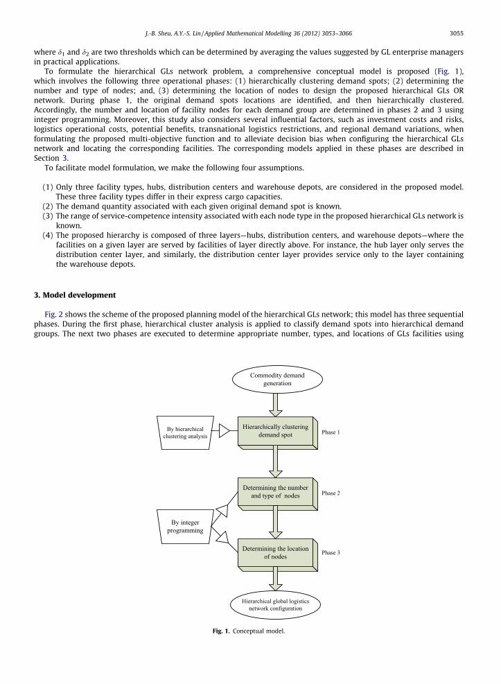
To formulate the hierarchical GLs network problem, a comprehensive conceptual model is proposed (Fig. 1),which involves the following three operational phases: (1) hierarchically clustering demand spots; (2) determining thenumber and type of nodes; and, (3) determining the location of nodes to design the proposed hierarchical GLs ORnetwork. During phase 1, the original demand spots locations are identified, and then hierarchically clustered.Accordingly, the number and location of facility nodes for each demand group are determined in phases 2 and 3 usinginteger programming. Moreover, this study also considers several influential factors, such as investment costs and risks,logistics operational costs, potential benefits, transnational logistics restrictions, and regional demand variations, whenformulating the proposed multi-objective function and to alleviate decision bias when configuring the hierarchical GLsnetwork and locating the corresponding facilities. The corresponding models applied in these phases are described inSection 3.

To facilitate model formulation, we make the following four assumptions.

(1) Only three facility types, hubs, distribution centers and warehouse depots, are considered in the proposed model.These three facility types differ in their express cargo capacities.

(2) The demand quantity associated with each given original demand spot is known.(3) The range of service-competence intensity associated with each node type in the proposed hierarchical GLs network is

known.(4) The proposed hierarchy is composed of three layers—hubs, distribution centers, and warehouse depots—where the

facilities on a given layer are served by facilities of layer directly above. For instance, the hub layer only serves thedistribution center layer, and similarly, the distribution center layer provides service only to the layer containingthe warehouse depots.

3. Model development

Fig. 2 shows the scheme of the proposed planning model of the hierarchical GLs network; this model has three sequentialphases. During the first phase, hierarchical cluster analysis is applied to classify demand spots into hierarchical demandgroups. The next two phases are executed to determine appropriate number, types, and locations of GLs facilities using

Fig. 1. Conceptual model.

Fig. 2. Scheme of the proposed model.


the proposed integer programming model. The details of the developmental procedures associated with phases 1, 2, and 3are presented in the following three subsections.

3.1. Demand-spot hierarchical cluster analysis

The hierarchical cluster analysis (Fig. 3) is composed of the following three steps: (1) selection of distance metrics; (2)variable standardization; and, (3) hierarchical clustering. The primary steps executed are as follows.

During the first step (i.e., selection of distance metrics), hierarchical cluster analysis considers each given object i as apoint in a multi-dimensional space characterized by two attributes—the amount of inbound (r1

i ) and outbound (r2i ) cargo

associated with object i. The distance between two objects is measured to determine the similarity among objects in termsof object attributes. Thus, the choice of a distance metric is the initial step in hierarchical cluster analysis. Although variousdistance metrics exist, such as Euclidean distance, Mahalanobis distance, city block distance, and Minkovski distance, Euclid-ean distance is utilized in this study as it is the most common and intuitive measure used in literature [19] when focusing onfacility location.

The second step (i.e., variable standardization) standardizes specified attributes. Variable standardization is an importantstep in hierarchical cluster analysis, since differences in units and magnitude of variance between attributes influence

Fig. 3. Conceptual framework for cluster analysis.


computational results of distance metrics. Therefore, each attribute rpi type is standardized; herein, the standardized attri-

bute (~rpi ) is given by

~rpi ¼

rpi � r�p

Sp ; ð1Þ

where r�p and Sp are the mean and standard deviation of rpi , respectively, and are given by

r�p ¼PN

i¼1rpi

N; ð2Þ

Sp ¼PN

i¼1ðrpi � r�pÞ

N � 1

" #12

; ð3Þ

where N is the number of customer demand spots from original data.After measuring the distance metrics and standardizing variables, the final step is hierarchical clustering. Since the

purpose of hierarchical cluster analysis is to combine objects into groups or hierarchical clusters, some method-basedrules are required to determine how to form these hierarchical clusters. In reality, some common centroid algorithms,such as the single-linkage method, the complete-linkage method, average-linkage method and Ward method, can beused for hierarchical clustering [20]. The single-linkage method is adopted as its computational process is generallyshorter than that of the other methods. In the single-linkage method, the distance between two clusters is theminimum distance between all possible object pairs in two clusters. The Euclidean distance matrix (M) can thenbe constructed, as in Eq. (4), where each element (xij) represents the distance between a given cluster pair such asi and j

M ¼

x11 x12 � � � x1i

x21 x22 � � � x2i

. .. . .

. ... . .

.

xi1 xi2 � � � xij

26666664

37777775

i�j

; xij � 0; if i ¼ j; xij ¼ xji; if i – j: ð4Þ

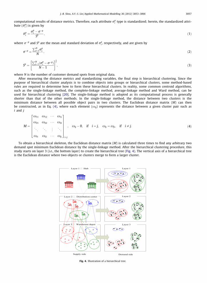
To obtain a hierarchical skeleton, the Euclidean distance matrix (M) is calculated three times to find any arbitrary twodemand spot minimum Euclidean distance by the single-linkage method. After the hierarchical clustering procedure, thisstudy starts on layer 3 (i.e., the bottom layer) to create the hierarchical tree (Fig. 4). The vertical axis of a hierarchical treeis the Euclidean distance where two objects or clusters merge to form a larger cluster.

Fig. 4. Illustration of a hierarchical tree.


3.2. Facility network configurations

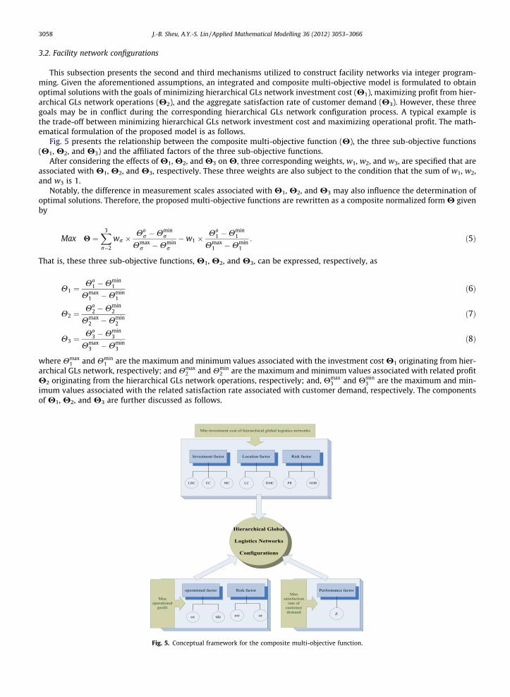
This subsection presents the second and third mechanisms utilized to construct facility networks via integer program-ming. Given the aforementioned assumptions, an integrated and composite multi-objective model is formulated to obtainoptimal solutions with the goals of minimizing hierarchical GLs network investment cost (H1), maximizing profit from hier-archical GLs network operations (H2), and the aggregate satisfaction rate of customer demand (H3). However, these threegoals may be in conflict during the corresponding hierarchical GLs network configuration process. A typical example isthe trade-off between minimizing hierarchical GLs network investment cost and maximizing operational profit. The math-ematical formulation of the proposed model is as follows.

Fig. 5 presents the relationship between the composite multi-objective function (H), the three sub-objective functions(H1, H2, and H3) and the affiliated factors of the three sub-objective functions.

After considering the effects of H1, H2, and H3 on H, three corresponding weights, w1, w2, and w3, are specified that areassociated with H1, H2, and H3, respectively. These three weights are also subject to the condition that the sum of w1, w2,and w3 is 1.

Notably, the difference in measurement scales associated with H1, H2, and H3 may also influence the determination ofoptimal solutions. Therefore, the proposed multi-objective functions are rewritten as a composite normalized form H givenby

Max H ¼X3

r¼2

wr �Ho

r �Hminr

Hmaxr �Hmin

r

�w1 �Ho

1 �Hmin1

Hmax1 �Hmin

1

: ð5Þ

That is, these three sub-objective functions, H1, H2, and H3, can be expressed, respectively, as

H1 ¼Ho

1 �Hmin1

Hmax1 �Hmin

1

ð6Þ

H2 ¼Ho

2 �Hmin2

Hmax2 �Hmin

2

ð7Þ

H3 ¼Ho

3 �Hmin3

Hmax3 �Hmin

3

ð8Þ

where Hmax1 and Hmin

1 are the maximum and minimum values associated with the investment cost H1 originating from hier-archical GLs network, respectively; and Hmax

2 and Hmin2 are the maximum and minimum values associated with related profit

H2 originating from the hierarchical GLs network operations, respectively; and, Hmax3 and Hmin

3 are the maximum and min-imum values associated with the related satisfaction rate associated with customer demand, respectively. The componentsof H1, H2, and H3 are further discussed as follows.

Fig. 5. Conceptual framework for the composite multi-objective function.


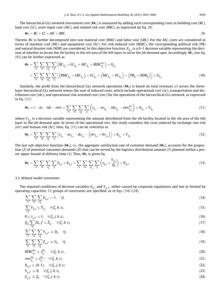
The hierarchical GLs network investment cost (H1) is measured by adding such corresponding costs as building cost (BC),land cost (LC), asset input cost (AIC), and related risk cost (RRC), as expressed by Eq. (9)

H1 ¼ BC þ LC þ AIC þ RRC: ð9Þ

Therein, BC is further decomposed into raw material cost (RMC) and labor cost (LBC). For the AIC, costs are considered interms of machine cost (MC) and equipment cost (EC). For risk-induced cost (RERC), the corresponding political risk (PR)and natural disaster risk (NDR) are considered. In this objective function, Xish ;j

is a 0–1 decision variable representing the deci-sion of whether to locate the ith facility in the sth area of the hth layer to serve the jth demand spot. Accordingly, H1 (see Eq.(9)) can be further expressed as

H1 ¼X8s

X8h

X8ish

X8j

BCish;jþ LCish;j

þ AICish;jþ RERCH1

ish

� �� Xish;j

¼X8s

X8h

X8ish

X8j

RMCish;jþ LBCish;j

� �þ LCish;j

þ MCish;jþ ECish;j

� �þ PRish

þ NDRish

� �j k� Xish;j

: ð10Þ

Similarly, the profit from the hierarchical GLs network operations (H2) is based on total revenues (r) across the three-layer hierarchical GLs network minus the sum of induced costs, which include operational cost (oc), transportation and dis-tribution cost (tdc), and operational risk-oriented cost (rorc) for the operations of the hierarchical GLs network, as expressedin Eq. (11)

H2 ¼ r � oc � tdc � rorc ¼X8s

X8h

X8ish

X8j

rish;j� ocish;j

� tdcish;j� rorcH2

ish;j

� �� Xish;j

� Yish;jð11Þ

where Yish ;jis a decision variable representing the amount distributed from the ith facility located in the sth area of the hth

layer to the jth demand spot. In terms of the operational rorc, this study considers the costs induced by exchange rate risk(err) and human risk (hr); thus, Eq. (11) can be rewritten as

H2 ¼X8s

X8h

X8ish

X8j

rish;j� ocish;j

� dcish;j� errish;j

þ hrish;j

� �j k� Xish;j

� Yish;j: ð12Þ

The last sub-objective function (H3), i.e., the aggregate satisfaction rate of customer demand (H3), accounts for the propor-tion (Z) of potential consumer demands (D) that can be served by the logistics distribution amount (Y) planned within a pre-set upper bound of delivery time (�t). Thus, H3 is given by

H3 ¼X8s

X8h

X8ish

X8j

Zish ;j� Xish ;j

¼X8s

X8h

X8ish

X8j

tish ;j�

Yish ;j

Dj

� �� Xish ;j

: ð13Þ

3.3. Related model constraints

The required conditions of decision variables Xish ;jand Yih ;j

s ; either caused by corporate regulations and law or limited byoperating capacities, 11 groups of constraints are specified, as in Eqs. (14)–(24).
X
8s

X8h

X8ish

Xih ;js ¼ 1; 8j; ð14Þ

X8j

Yish ;j6 Yish

; 8ðish; h; sÞ; ð15Þ

0 6 tih ;js 6 �t; 8ðis

h; j;h; sÞ; ð16ÞUish

X8j

Zih; js6 Zish

; 8ðish;h; sÞ; ð17Þ

X8s

X8h

X8ish

Yih ;js P Dj; 8j; ð18Þ

X8s

X8h

X8ish

Zih ;js P Gj; 8j; ð19Þ

RERCH1ish6 dH1

ish; 8ðis

h;h; sÞ; ð20Þ

rorcH2ish6 dH2

ish; 8ðis

h; h; sÞ; ð21Þ

Xih ;js 2 f0;1g; 8ðis

h; j;h; sÞ; ð22ÞYih ;j

s P 0; 8ðish; j; h; sÞ; ð23Þ

Zih ;js P Zj; 8ðis

h; j;h; sÞ: ð24Þ


In Eq. (14), decision variable Xish ;jis specified to ensure that any demand spot is served by only one facility to avoid squan-

dering facility resources. Eq. (15) represents the corresponding upper bound limitation of the decision variable Yish ;j. Eqs. (16)

and (17) are the upper and lower bounds associated with derivative decision variable Zish ;jand parameter tish ;j

while consid-ering potential governmental regulations and basic requirements for international express delivery enterprise distributionresource allocation. Eqs. (18) and (19) represent the basic requirements for service levels in terms of in-bound logisticsand satisfaction rate of the customer associated with each given demand spot. Eqs. (20) and (21) are specified for the con-cerns of the maximum external and internal risks tolerated by enterprises. For example, the transnational investment of anenterprise may account for varied potential risks caused by uncertainties associated with either natural and artificial eventssuch as natural disasters, anomalous variations in exchange rates, and political risks. Therefore, the upper bounds of theRERCs are specified in the model.

In addition to the aforementioned constraints, all decision variables should be subject to the non-negative domain tomeet the basic requirement of a feasible solution. Correspondingly, all decision variables should be restricted to the real-value domain that is P0, and the others are 0–1 binary decision variables, as in Eqs. (22)–(24). Therefore, according tothe proposed model, the optimal solutions of decision variables together with these updated functions will determine thebest location and optimal distribution amount for each layer under the optimized system for hierarchical GLs network.

4. Numerical study

4.1. Experimental design and data collection

The numerical study is focused on the case of an international express delivery company, DHL. Its current internationalexpress cargo capacity is more than 1 billion ton, accounting for nearly 30% of all international express cargo. Additionally,the DHL global network has four head offices. Each head office has 2–5 hubs in operation; thus, 12 hubs are considered.Based on the study scope and limitations in acquiring real data, we assume the international express delivery demandsare from Taiwan, China, and the USA, which, as mentioned, are the three dominant international express delivery cargosources worldwide. Furthermore, as cross-strait direct shipping is prohibited, transnational cargo transportation betweenTaiwan and China is not considered in this case study.

This case study considered three regions, Taiwan, China, and the USA, for the GLs network configurations. Therein, 15 ori-ginal demand spots are located in Taiwan, 116 original demand spots are in China, and 260 original demand spots in the USAwhere these demand spots are determined using local population data. The thresholds d1 and d2 associated with the facilityservice-competence intensity index (q) were determined by averaging the values suggested by GL enterprise managers wereused in the case study. Based on the predetermined thresholds and proposed facility identification rules, 3 original demandspots in Taiwan (e.g. Taipei, Taichung, and Kaohsiung) were chosen as candidates for the consideration of locating hubs. Sim-ilarly, there are 15 and 36 original demand spots chosen as candidates for locating hubs in China and the USA, respectively.Accordingly, the problem scope has 3429 decision variables subject to 1068 constraints.

The local express-delivery demand was estimated based on input data. Notably, the primary purpose of this numericalstudy is to demonstrate the applicability of the proposed approach to a simplified case (DHL). Due to difficulties in collectingreal demand data for each demand spot, this study utilized a simple data processing procedure. Processed demand data werethen used as the common database to assess the relative performance of the proposed model by comparing it with the exist-ing performance of DHL.

First, this study collected data for local populations of these demand spots and the corresponding gross domestic product(GDP) data from databases in Taiwan, China, and the USA. International express delivery demand associated with each ori-ginal demand spot was then approximated using a proportion of GDP and the corresponding local population.

The next step generated a four-tier GLs hierarchical network, including the three main regions (first tier), sub-regions(second tier), the local area (third tier), and original demand spots (fourth tier) based on geographical relationships. Table 1presents hierarchical cluster results.

Notably, errors in demand data approximation may exist. However, this issue may not be of major concern based on studyscope and its primary purpose.

4.2. Setting parameters

Model parameters estimated in this scenario are classified into (1) cost-related parameters, (2) risk-related parameters,and (3) boundary conditions. These parameters were estimated using interview survey data and corresponding statistics.

Practically, estimating cost-related parameters, such as unit operational cost, directly from reported statistical data is dif-ficult due to business confidentiality and security concerns. Therefore, interviews with key staff in express operations andlogistics-related sectors of DHL were conducted to collect real data. The interviews utilized both open-ended and closedquestions regarding existing strategies in express air delivery and logistics management, as well as potential limitations.A questionnaire was designed based on the need to estimate cost-related parameters of the model. For example, given a costitem, the corresponding survey respondent was asked to measure unit cost within an acceptable range. Analytical results ofinterviews were then processed to determine unit operational costs and boundaries using uniform distributions with ranges

Table 1Hierarchical cluster results of the proposed GLs network.

1st tier 2nd tier 3rd tierRegion Sub-regions Local area (Original demand spots)

Taiwan 1. Northern Taipei (6), Keelung (1), Taoyuan (2), Hsinchu (1)2. Central andsouthern

Taichung (1), Chiayi (1), Tainan (1), Kaohsiung (2)

China 1. Northern China Beijing (1), Tianjin (1), Hebei (10), Shanxi (3), Inner Mongolia (2)2. Central China Henan (9), Hubei (3), Hunan(7)3. Southern China Guangdong (10), Hainan (1), Hong Kong (1), Macao (1), Guangxi (3)4. Eastern China Shanghai (1), Shandong (5), Jiangsu (11), Anhui (6), Zhejiang (3), Jiangxi (1), Fujian (3)5. Nothern-eastChina

Liaoning (11), Jilin (3), Heilongjiang (5)

6. Northern-westChina

Shaanxi (2), Gansu (1), Qinghai (1), Ningxia (1), Xinjiang (2)

7. Southern-westChina

Chongqing (1), Sichuan (3), Yunnan (1), Guizhou (2), Tibet (1)

TheUSA

1. New England Connecticut (5), Maine (1), Massachusetts (5), New Hampshire (1), Rhode Island (1), Vermont (1)2. Atlantic Delaware (1), District of Columbia (1), Florida (17), Georgia (5), Maryland (1), New Jersey (4), New York (5), North

Carolina (7), Pennsylvania (4), South Carolina (2), Virginia (9), West Virginia (1)3. Mid-west Illinois (7), Indiana (4), Iowa (2), Michigan (7), Minnesota (2), Nebraska (2), North Dakota (1), Ohio (6), South Dakota

(1), Wisconsin (3)4. South Alabama (4), Arkansas (1), Kentucky (2), Kansas (5), Louisiana (4), Mississippi (1), Missouri (4), Oklahoma (3),

Tennessee (5), Texas (25)5. Rockies Arizona (9), Colorado (9), Idaho (1), Montana (1), New Mexico(1), Utah(2), Wyoming (1)6. Pacific Alaska (1), California (62), Hawaii (1), Nevada (4), Oregon (3), Washington (5)

Note: the number inside parentheses in the third-tier column is the number of original demand spots.

Table 2Estimated parameters of the minimum cost objective function.

Region Type of cost (US$)

RMCish ;jLBCish ;j

LCish ;jMCish ;j

ECish ;jPRish ;j

NDRish ;j

Taiwan 3 2 100 8 6 50 85China 6 6 110 4 9 35 60The USA 5 4 100 9 7 40 75


bounded by the estimated upper and lower bounds in the profit-maximization objective function and corresponding con-straints, respectively.

Risk-related parameters estimated in this scenario aim at the unit increments of money (m) risks for environmental riskcost and operational risk cost induced by the hierarchical GLs network configuration. Corresponding parameters are classi-

fied into and associated with the following five activities: (1) government stability (mgsish

); (2) earthquake (meish

); (3) flood (mfish

);

(4) exchange rate (merish

); and (5) personnel skills (mpsish

). Among these risk-related parameters, mgsish

and mpsish

are associated withthe corresponding artificial organization and behavior; the others are influenced by natural disasters and operational situ-ations in the resulting hierarchical GLs network. As mentioned, a unit increase in risk-induced penalty refers to the monetaryvalue of a particular penalty caused by the unit of a given physical amount associated with a particular activity.

According to literature, a democratic or communist regime may affect aspirations and freedoms related to businesssecrets for an international express delivery enterprise. Conveniently, mgs

ishwas derived from comparative measures of free-

dom developed by the Freedom House and Business Environment Risk Intelligence [21].To estimate unit incremental risks me

ishand mf

ishfor natural disasters, this study first averaged aggregate earthquake and

flood damage costs of these three regions over the last 30 years using historical data provided by central governments. Sec-ond, aggregate damage costs caused by earthquakes and floods were measured using the averaged aggregate earthquake andflood damage costs multiplied by the ratio of natural disaster frequency over the last 30 years.

Conversely, exchange rate risk (err) may depend on foreign reserves, exchange law, and foreign debt. Therefore, this studyestimated the exchange-oriented risk (mer

ish) by approximating the corresponding comparative measures of exchange risk

from BERI, which is similar to the concept of political risk cost for the three regions. Here, according to the proposed method,exchange risk can be expressed by the amount of foreign debt divided by the amount of foreign reserves. In this case study,statistics for foreign debt and foreign reserves for these three governments were used to estimate the correspondingexchange risk.

Similar to risks induced by the government stability, personnel skill risk (ps) can be caused by either Democracy or Com-munism. Accordingly, (mps

ish) was estimated using comparative measures of freedom developed by the Freedom House and


BERI for workers and society. Notably, parameter mpsish

may vary with race; particularly, whites currently have an advanta-geous position worldwide.

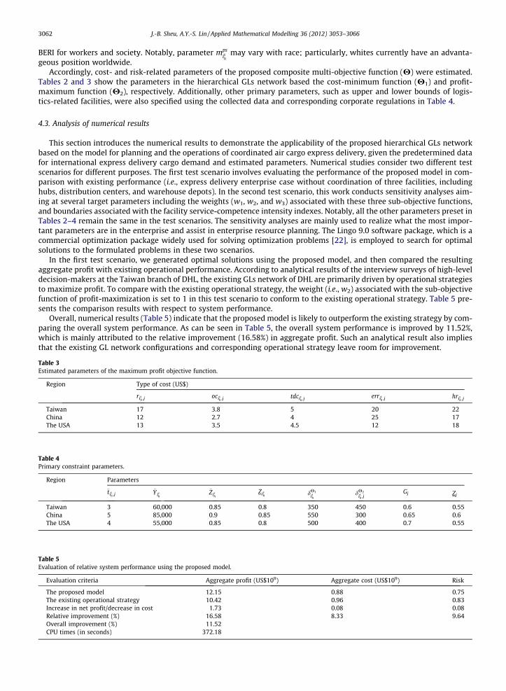
Accordingly, cost- and risk-related parameters of the proposed composite multi-objective function (H) were estimated.Tables 2 and 3 show the parameters in the hierarchical GLs network based the cost-minimum function (H1) and profit-maximum function (H2), respectively. Additionally, other primary parameters, such as upper and lower bounds of logis-tics-related facilities, were also specified using the collected data and corresponding corporate regulations in Table 4.

4.3. Analysis of numerical results

This section introduces the numerical results to demonstrate the applicability of the proposed hierarchical GLs networkbased on the model for planning and the operations of coordinated air cargo express delivery, given the predetermined datafor international express delivery cargo demand and estimated parameters. Numerical studies consider two different testscenarios for different purposes. The first test scenario involves evaluating the performance of the proposed model in com-parison with existing performance (i.e., express delivery enterprise case without coordination of three facilities, includinghubs, distribution centers, and warehouse depots). In the second test scenario, this work conducts sensitivity analyses aim-ing at several target parameters including the weights (w1, w2, and w3) associated with these three sub-objective functions,and boundaries associated with the facility service-competence intensity indexes. Notably, all the other parameters preset inTables 2–4 remain the same in the test scenarios. The sensitivity analyses are mainly used to realize what the most impor-tant parameters are in the enterprise and assist in enterprise resource planning. The Lingo 9.0 software package, which is acommercial optimization package widely used for solving optimization problems [22], is employed to search for optimalsolutions to the formulated problems in these two scenarios.

In the first test scenario, we generated optimal solutions using the proposed model, and then compared the resultingaggregate profit with existing operational performance. According to analytical results of the interview surveys of high-leveldecision-makers at the Taiwan branch of DHL, the existing GLs network of DHL are primarily driven by operational strategiesto maximize profit. To compare with the existing operational strategy, the weight (i.e., w2) associated with the sub-objectivefunction of profit-maximization is set to 1 in this test scenario to conform to the existing operational strategy. Table 5 pre-sents the comparison results with respect to system performance.

Overall, numerical results (Table 5) indicate that the proposed model is likely to outperform the existing strategy by com-paring the overall system performance. As can be seen in Table 5, the overall system performance is improved by 11.52%,which is mainly attributed to the relative improvement (16.58%) in aggregate profit. Such an analytical result also impliesthat the existing GL network configurations and corresponding operational strategy leave room for improvement.

Table 3Estimated parameters of the maximum profit objective function.

Region Type of cost (US$)

rish ;jocish ;j

tdcish ;jerrish ;j

hrish ;j

Taiwan 17 3.8 5 20 22China 12 2.7 4 25 17The USA 13 3.5 4.5 12 18

Table 4Primary constraint parameters.

Region Parameters

�tish ;j�Yish

�ZishZish dH1

ishdH2

ish ;jGj Zj

Taiwan 3 60,000 0.85 0.8 350 450 0.6 0.55China 5 85,000 0.9 0.85 550 300 0.65 0.6The USA 4 55,000 0.85 0.8 500 400 0.7 0.55

Table 5Evaluation of relative system performance using the proposed model.

Evaluation criteria Aggregate profit (US$109) Aggregate cost (US$109) Risk

The proposed model 12.15 0.88 0.75The existing operational strategy 10.42 0.96 0.83Increase in net profit/decrease in cost 1.73 0.08 0.08Relative improvement (%) 16.58 8.33 9.64Overall improvement (%) 11.52CPU times (in seconds) 372.18

Table 6Results of sensitivity analysis with respect to d1.

Country Threshold d1 increment (%)Variations in service-competence intensity

�50% �25% 0 +25% +50%

Taiwan Kaohsiung, Keelung,Taichung, Taipei

Kaohsiung, Taichung,Taipei

Kaohsiung, Taichung,Taipei

Kaohsiung, Taipei Taipei

4 3 3 2 1

China Harbin, Shenyang,Changchun, Chongqing,Shanghai, Nanjing,Chengdu, Wuhan,Changsha, Beijing,Tianjin, Xi’an, Taiyuan,Guangzhou, Hong Kong,Dalian, Jinan, Hangzhou,Jilin, Shijiazhuang

Harbin, Shenyang,Changchun, Chongqing,Shanghai, Nanjing,Chengdu, Wuhan,Changsha, Beijing,Tianjin, Xi’an, Taiyuan,Guangzhou, Hong Kong,Dalian, Hangzhou,Shijiazhuang

Harbin, Shenyang,Changchun, Chongqing,Shanghai, Nanjing,Chengdu, Wuhan,Changsha, Beijing,Tianjin, Xi’an, Taiyuan,Guangzhou, Hong Kong

Harbin, Changchun,Chongqing, Shanghai,Nanjing, Chengdu,Beijing, Tianjin, Xi’an,Taiyuan, Guangzhou,Hong Kong

Chongqing, Shanghai,Nanjing, Beijing,Tianjin, Guangzhou,Hong Kong

20 18 15 12 7

TheUSA

New York, Philadelphia,Washington, Baltimore,Detroit, Indianapolis,Columbus, Milwaukee,Minneapolis, Omaha,Chicago, Los Angeles, SanDiego, San Jose, Portland,San Francisco, Seattle,Charlotte, Virginia Beach,Louisville-Jefferson,Memphis, Nashville,Jacksonville, OklahomaCity, Austin, El Paso, FortWorth, Houston, SanAntonio, Dallas, Boston,Phoenix, Tucson, LasVegas, Denver,Albuquerque, Atlanta,New Orleans, Long Beach,Oakland, Kansas City, St.Louis, Buffalo, ColoradoSprings, Honolulu, Miami

New York, Philadelphia,Washington, Baltimore,Detroit, Indianapolis,Columbus, Milwaukee,Minneapolis, Omaha,Chicago, Los Angeles, SanDiego, San Jose, Portland,San Francisco, Seattle,Charlotte, Virginia Beach,Louisville-Jefferson,Memphis, Nashville,Jacksonville, OklahomaCity, Austin, El Paso, FortWorth, Houston, SanAntonio, Dallas, Boston,Phoenix, Tucson, LasVegas, Denver,Albuquerque, Atlanta,New Orleans, Long Beach,Oakland, Kansas City, St.Louis

New York, Philadelphia,Washington, Baltimore,Detroit, Indianapolis,Columbus, Milwaukee,Minneapolis, Omaha,Chicago, Los Angeles, SanDiego, San Jose, Portland,San Francisco, Seattle,Charlotte, Virginia Beach,Louisville-Jefferson,Memphis, Nashville,Jacksonville, OklahomaCity, Austin, El Paso, FortWorth, Houston, SanAntonio, Dallas, Boston,Phoenix, Tucson, LasVegas, Denver,Albuquerque

New York, Philadelphia,Washington, Baltimore,Detroit, Indianapolis,Columbus, Milwaukee,Minneapolis, Chicago, LosAngeles, San Diego,Portland, San Francisco,Seattle, Charlotte,Oklahoma City, Houston,Dallas, Boston, Phoenix

New York, Philadelphia,Washington, Detroit,Columbus, Chicago, LosAngeles, San Diego,Portland, San Francisco,Seattle, Houston,Boston

46 42 36 21 13


In the second test scenario, we conducted sensitivity analyses with respect to the following four parameters—(1) thethreshold (d1) associated with the facility service-competence intensity index for determination of hub locations, (2) originaldemand (Dj), (3) upper and lower bounds of the satisfaction rate of customer demand (Zish

; Zish), and (4) the weights associated

with the three sub-objective functions. Therein, the combination of w1 = w2 = w3 = 13 was chosen for all cases except for the

sensitivity analysis with respect to these weights. We summarized the results of sensitivity analysis with respect to d1 inTable 6, and the others in Table 7. The following implications are provided based on the analytical results of Tables 6 and 7.

(1) A GL enterprise is allowed to loosen the facility allocation threshold by choosing a lower value of d1 for the determi-nation of hub locations if the enterprise has enough capital and human resources allocated in GL network configura-tions. As can be seen in Table 6, the numbers of hubs that can be located in Taiwan, China, and the US increase up to 4,20, and 46, respectively, when the threshold d1 decreases by 50%.

(2) The reduction of original demands may contribute significantly to the aggregate improvement in system performance.The aggregate cost of the hierarchical GLs network can be improved by 32.93% when original demands are reduced by50%.

(3) Given the necessity of increasing the satisfactory rate of customer by 50% to replace other situations, the aggregateperformance of the proposed hierarchical GLs network improves 31.45% than original situation.

(4) As revealed by sensitivity analysis, adjusting the corresponding weights associated with the three sub-objective func-tions have a significant effect on enhancing overall improvement. The weights associated with the profit sub-objectivefunction w2 is equals 1, then the aggregate profit is 12.15 � 109 US dollars and is larger than the other situation.

Overall, numerical results are indicative of the potential advantages of the proposed hierarchical GLs network, and theimportance of appropriate hierarchical GLs network configuration strategies in determining system performance.

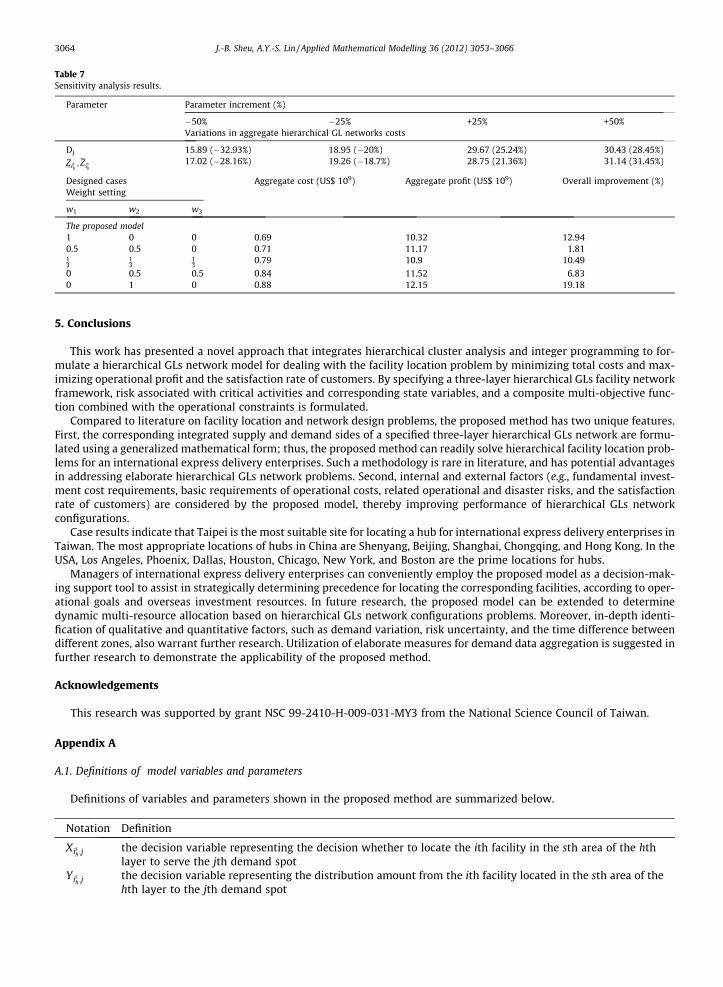
Table 7Sensitivity analysis results.

Parameter Parameter increment (%)

�50% �25% +25% +50%Variations in aggregate hierarchical GL networks costs

Dj 15.89 (�32.93%) 18.95 (�20%) 29.67 (25.24%) 30.43 (28.45%)Zish; Zish

17.02 (�28.16%) 19.26 (�18.7%) 28.75 (21.36%) 31.14 (31.45%)

Designed casesWeight setting

Aggregate cost (US$ 109) Aggregate profit (US$ 109) Overall improvement (%)

w1 w2 w3

The proposed model1 0 0 0.69 10.32 12.940.5 0.5 0 0.71 11.17 1.8113

13

13

0.79 10.9 10.49

0 0.5 0.5 0.84 11.52 6.830 1 0 0.88 12.15 19.18


5. Conclusions

This work has presented a novel approach that integrates hierarchical cluster analysis and integer programming to for-mulate a hierarchical GLs network model for dealing with the facility location problem by minimizing total costs and max-imizing operational profit and the satisfaction rate of customers. By specifying a three-layer hierarchical GLs facility networkframework, risk associated with critical activities and corresponding state variables, and a composite multi-objective func-tion combined with the operational constraints is formulated.

Compared to literature on facility location and network design problems, the proposed method has two unique features.First, the corresponding integrated supply and demand sides of a specified three-layer hierarchical GLs network are formu-lated using a generalized mathematical form; thus, the proposed method can readily solve hierarchical facility location prob-lems for an international express delivery enterprises. Such a methodology is rare in literature, and has potential advantagesin addressing elaborate hierarchical GLs network problems. Second, internal and external factors (e.g., fundamental invest-ment cost requirements, basic requirements of operational costs, related operational and disaster risks, and the satisfactionrate of customers) are considered by the proposed model, thereby improving performance of hierarchical GLs networkconfigurations.

Case results indicate that Taipei is the most suitable site for locating a hub for international express delivery enterprises inTaiwan. The most appropriate locations of hubs in China are Shenyang, Beijing, Shanghai, Chongqing, and Hong Kong. In theUSA, Los Angeles, Phoenix, Dallas, Houston, Chicago, New York, and Boston are the prime locations for hubs.

Managers of international express delivery enterprises can conveniently employ the proposed model as a decision-mak-ing support tool to assist in strategically determining precedence for locating the corresponding facilities, according to oper-ational goals and overseas investment resources. In future research, the proposed model can be extended to determinedynamic multi-resource allocation based on hierarchical GLs network configurations problems. Moreover, in-depth identi-fication of qualitative and quantitative factors, such as demand variation, risk uncertainty, and the time difference betweendifferent zones, also warrant further research. Utilization of elaborate measures for demand data aggregation is suggested infurther research to demonstrate the applicability of the proposed method.

Acknowledgements

This research was supported by grant NSC 99-2410-H-009-031-MY3 from the National Science Council of Taiwan.

Appendix A

A.1. Definitions of model variables and parameters

Definitions of variables and parameters shown in the proposed method are summarized below.

Notation
Definition
Xish ;j

the decision variable representing the decision whether to locate the ith facility in the sth area of the hthlayer to serve the jth demand spot

Yish ;j

the decision variable representing the distribution amount from the ith facility located in the sth area of thehth layer to the jth demand spot


Appendix A (continued)

Notation
Definition
Zish ;j
the derivative decision variable about the satisfied rate of customer demand associated with the ith facility inthe sth area and the hth layer for the jth demand
BCish ;j
the building cost associated with the ith facility in the sth area and the hth layer for the jth demand
LCish ;j
the land cost associated with the ith facility in the sth area and the hth layer for the jth demand
AICish ;j
the asset input cost associated with the ith facility in the sth area and the hth layer for the jth demand
RERCH1

ish ;j
the related environment risk cost induced in H1 associated with the ith facility in the sth area and the hthlayer for the jth demand
RMCish ;j
the raw material cost associated with the ith facility in the sth area and the hth layer for the jth demand
LBCish ;j
the labor cost associated with the ith facility in the sth area and the hth layer for the jth demand
MCish ;j
the machine cost associated with the ith facility in the sth area and the hth layer for the jth demand
ECish ;j
the equipment cost associated with the ith facility in the sth area and the hth layer for the jth demand
PRish ;j
the political risk associated with the ith facility in the sth area and the hth layer for the jth demand
NDRish ;j
the natural disaster risk associated with the ith facility in the sth area and the hth layer for the jth demand
rish ;j
the aggregate revenue associated with the ith facility in the sth area and the hth layer for the jth demand
ocish ;j
the aggregate operational cost associated with the ith facility in the sth area and the hth layer for the jthdemand
dcish ;j
the aggregate distribution cost associated with the ith facility in the sth area and the hth layer for the jthdemand
rorcH2

ish ;j
the related operational risk cost induced in H2 associated with the ith facility in the sth area and the hth layerfor the jth demand
errish ;j
the exchange rate risk associated with the ith facility in the sth area and the hth layer for the jth demand
hrish ;j
the human risk associated with the ith facility in the sth area and the hth layer for the jth demand
tish ;j
the unit upper bound time during the plan period to guarantee and content customer demand associatedwith the ith facility in the sth area and the hth layer for the jth demand
Dj
the jth original demand for amount of distribution �Yish
the upper bound providing distribution amount with the ith facility in the sth area and the hth layer
�Zish
the upper satisfied rate bound of customer demand associated with the ith facility in the sth area and the hthlayer

Zish
the lower satisfied rate bound of customer demand associated with the ith facility in the sth area and the hthlayer
Gj
the jth lower bound of the satisfaction rate of customer demand
dH1

ish ;j
the upper bound for the related environment risk cost induced in H1 associated with the ith facility in the stharea and the hth layer for the jth demand
dH2

ish ;j
the upper bound the related operational risk cost induced in H2 associated with the ith facility in the sth areaand the hth layer for the jth demand
Zj
the lower satisfied rate bound of the jth customer demand mgs
ish
the money risk for government stability associated with the ith facility in the sth area and the hth layer forthe jth demand
meish

the money risk for earthquake associated with the ith facility in the sth area and the hth layer for the jthdemand

mfish

the the money risk for flood associated with the ith facility in the sth area and the hth layer for the jthdemand

merish

the the money risk for exchange rate associated with the ith facility in the sth area and the hth layer for thejth demand

mpsish

the the money risk for personnel skill associated with the ith facility in the sth area and the hth layer for thejth demand

References

[1] T. Miller, D. Wise, L. Clair, Transport network design and mode choice modeling for automobile distribution: a case study, Location Sci. 4 (1996) 37–48.[2] T.G. Crainic, Service network design in freight transportation, Eur. J. Oper. Res. 122 (2000) 272–288.[3] S. Melkote, M.S. Daskin, Capacitated facility location/network design problems, Eur. J. Oper. Res. 129 (2001) 481–495.[4] A. Cakravastia, I.S. Toha, N. Nakamura, A two-stage model for the design of supply chain networks, Int. J. Prod. Econ. 80 (2002) 231–248.[5] V. Jayaraman, A. Ross, A simulated annealing methodology to distribution network design and management, Eur. J. Oper. Res. 144 (2003) 629–645.[6] Z. Drezner, G.O. Wesolowsky, Network design: selection and design of links and facility location, Transp. Res. Part A 37 (2003) 241–256.


[7] D. Ambrosino, M.G. Scutella, Distribution network design: new problems and related models, Eur. J. Oper. Res. 165 (2005) 610–624.[8] J.R. Current, C.S. Revelle, J.L. Cohon, The hierarchical design problem, Eur. J. Oper. Res. 27 (1986) 57–66.[9] N.G.F. Sancho, The hierarchical network design problem with multiple primary paths, Eur. J. Oper. Res. 96 (1996) 323–328.

[10] C.C. Lin, S.H. Chen, The hierarchical network design problem for time-definite express common carriers, Transp. Res. Part B 38 (2004) 271–283.[11] Y.W. Wan, R.K. Cheung, J. Liu, J.H. Tong, Warehouse location problems for airfreight forwarders: a challenge created by the airport relocation, J. Air

Transp. Manage. 4 (1998) 201–207.[12] C.C. Lin, Y.J. Lin, D.Y. Lin, The economic effects of center-to-center directs on hub-and-spoke for air express common carriers, J. Air Transp. Manage. 9

(2003) 255–265.[13] M. Wasner, G. Zapfel, An integrated multi-depot hub-location vehicle routing model for network planning of parcel service, Int. J. Prod. Econ. 90 (2004)

403–419.[14] A.A. Chaves, L. Lan, Hybrid algorithms with detection of promising areas for the prize collecting traveling salesman problem, in: International

Conference on Hybrid Intelligent Systems, IEEE Computer Society, 2005.[15] J.-B. Sheu, A novel dynamic resource allocation model for demand-responsive city logistics distribution operations, Transp. Res. Part E 42 (2006) 445–

472.[16] K.-M. Osei-Bryson, T.R. Inniss, A hybrid clustering algorithm, Comput. Oper. Res. 34 (2007) 3255–3269.[17] A. Nagurney, D. Matsypura, Global supply chain network dynamics with multicriteria decision-making under risk and uncertainty, Transp. Res. Part E

41 (2005) 585–612.[18] B. Groothedde, C. Ruijgrik, L. Tavasszy, Towards collaborative, intermodal hub networks: a case study in the fast moving consumer goods market,

Transp. Res. Part E 41 (2005) 567–583.[19] D. Afshartous, Y. Guan, A. Mehrotra, US Coast Guard air station location with respect to distress calls: a spatial statistics and optimization based

methodology, Eur. J. Oper. Res. 196 (2009) 1086–1096.[20] H. Ankara, S. Yerel, Determination of sampling errors in natural stone plates through single linkage cluster method, J. Mater. Process. Technol. 209

(2009) 2483–2487.[21] Business Environment Risk Intelligence (BERI), Business Risk Service Annual Report, vol. 3, December, 2008.[22] Lindo Systems Inc., LINGO user’s guide, LINDO SYSTEMS INC., 2004.

applied mathematical modelling · applied mathematical modelling 36 (2012) 3053–3066 ... the...

Documents