Mathematical Modeling and Engineering

Problem Solving

What are NUMERICAL METHODS?

Why do we need them?

Numerical Methods:

Algorithms that are used to obtain numerical solutions of

a mathematical problem.

Why do we need them?

1. No analytical solution exists,

2. An analytical solution is difficult to obtain

or not practical.

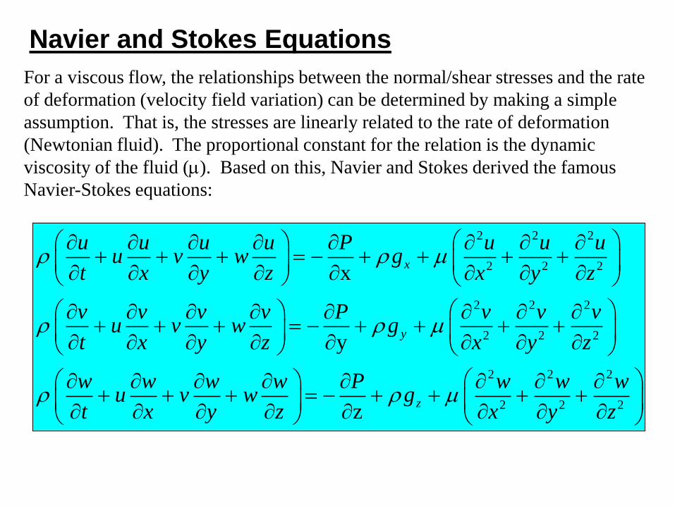
Navier and Stokes Equations

For a viscous flow, the relationships between the normal/shear stresses and the rate

of deformation (velocity field variation) can be determined by making a simple

assumption. That is, the stresses are linearly related to the rate of deformation

(Newtonian fluid). The proportional constant for the relation is the dynamic

viscosity of the fluid (m). Based on this, Navier and Stokes derived the famous

Navier-Stokes equations:

2 2 2

2 2 2

2 2 2

2 2 2

2 2 2

2 2 2

x

y

z

x

y

z

u u u u P u u uu v w g

t x y z x y z

v v v v P v v vu v w g

t x y z x y z

w w w w P w w wu v w g

t x y z x y z

m

m

m

5

Engineering Simulations

Finite element analysis (FEA) and product design services

Computational Fluid Dynamics (CFD)

Molecular Dynamics

Particle Physics

Earthquake simulations

Development of new products and performance improvement of existing

products

Benefits of Simulations

Cost savings by minimizing material usage.

Increased speed to market through reduced product development time.

Optimized structural performance with thorough analysis

Eliminate expensive trial-and-error.

Basic Needs in the Numerical Methods:

– Practical: Can be computed in a reasonable amount of time.

– Accurate:

• Good approximate to the true value,

• Information about the approximation error

(Bounds, error order,… ).

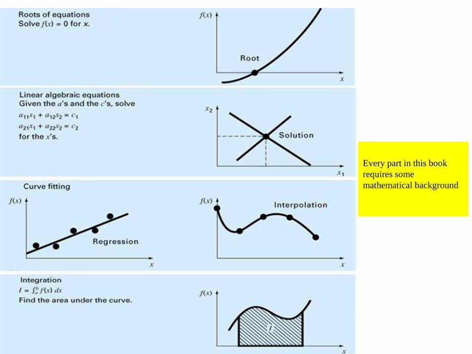
Every part in this book

requires some

mathematical background

Computers are great tools,

however, without fundamental understanding of engineering problems, they will be useless.

9

The engineering problem-solving process

Newton’s 2nd law

Conservation laws

10

Newton’s 2nd law of Motion

• “The time rate change of momentum of a body is equal

to the resulting force acting on it.”

• Formulated as F = m.a

F = net force acting on the body

m = mass of the object (kg)

a = its acceleration (m/s2)

• Some complex models may require more sophisticated

mathematical techniques than simple algebra

– Example, modeling of a falling parachutist:

FU = Force due to air resistance = -cv (c = drag

coefficient)

FD = Force due to gravity = mg

UD FFF

m

cvmg

dt

dv

cvF

mgF

FFF

m

F

dt

dv

U

D

UD

vm

cg

dt

dv

• This is a first order ordinary

differential equation. We would like to

solve for v (velocity).

• It can not be solved using algebraic

manipulation

• Analytical Solution:

If the parachutist is initially at rest

(v=0 at t=0), using calculus dv/dt can

be solved to give the result:

tmcec

gmtv )/(1)(

Independent

variableDependent

variable

ParametersForcing

function

Analytical Solution

tmcec

gmtv )/(1)(

t (sec.) V (m/s)

0 0

2 16.40

4 27.77

8 41.10

10 44.87

12 47.49

∞ 53.39

If v(t) could not be solved analytically, then

we need to use a numerical method to solve

it

g = 9.8 m/s2 c =12.5 kg/s

m = 68.1 kg

13

)()()(

lim........)()(

1

1

01

1

i

ii

ii

tii

ii

tvm

cg

tt

tvtv

t

v

dt

dv

tt

tvtv

t

v

dt

dv

))](([)()( 11 iiitttv

m

cgtvtv ii

This equation can be rearranged to yield

∆t = 2 sec

To minimize the error, use a smaller step size, ∆t

No problem, if you use a computer!

Numerical Solution

t (sec.) V (m/s)

0 0

2 19.60

4 32.00

8 44.82

10 47.97

12 49.96

∞ 53.39

t (sec.) V (m/s)

0 0

2 19.60

4 32.00

8 44.82

10 47.97

12 49.96

∞ 53.39

t (sec.) V (m/s)

0 0

2 16.40

4 27.77

8 41.10

10 44.87

12 47.49

∞ 53.39

m=68.1 kg c=12.5 kg/s

g=9.8 m/s

tmcec

gmtv )/(1)( ttv

m

cgtvtv

iii )]([)()( 1

∆t = 2 sec

Analytical

t (sec.) V (m/s)

0 0

2 17.06

4 28.67

8 41.95

10 45.60

12 48.09

∞ 53.39

∆t = 0.5 sec

t (sec.) V (m/s)

0 0

2 16.41

4 27.83

8 41.13

10 44.90

12 47.51

∞ 53.39

∆t = 0.01 sec

CONCLUSION: If you want to minimize

the error, use a smaller step size, ∆t

Numerical solutionvs.

Comparison of numerical and analytical solutions

Larger step size less accurate result

Smaller step size more steps (longer computing time)

Derive the mathematical equations that describes the fluid system below

• The rate of change in liquid stored in the tank is equal to the flow in

minus flow out.

• The resistance R may be written as

• Rearranging equation (2)

oi qqdt

dhC

(1)

0q

h

dQ

dHR (2)

R

hq 0 (3)

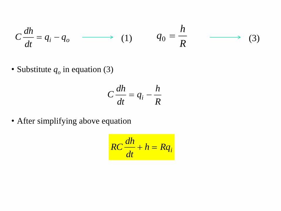
• Substitute qo in equation (3)

• After simplifying above equation

oi qqdt

dhC (1)

R

hq 0 (3)

R

hq

dt

dhC i

iRqhdt

dhRC

0M - M outin

SweatOutAir FecesSkinUrineMetabolismInAir DrinkFood

MetabolismInAir FoodSweatOutAir FecesSkinUrineDrink

L 2.13.005.012.04.02.035.04.1Drink

3out,3out,2in,1 AvQQ

233

out,3

out,2in,1

3 m 333.3m/s 6

/sm 20/sm 40

v

QQA

Special Problem 1

Schematic of a cart-pendulum system

Derive the equations of motion for the two-degree of freedom system.

In this system…….

It requires two coordinates, x and .

It requires two equations of motion:

1. The linear motion of the system.

2. The rotation of the pendulum.