Apply Radios to Improve the Operation of Electrical Protection

Shankar V. Achanta, Brian MacLeod, Eric Sagen, and Henry Loehner Schweitzer Engineering Laboratories, Inc.

Published in SEL Journal of Reliable Power, Volume 1, Number 2, October 2010

Originally presented at the 37th Annual Western Protective Relay Conference, October 2010

1

Apply Radios to Improve the Operation of Electrical Protection

Shankar V. Achanta, Brian MacLeod, Eric Sagen, and Henry Loehner, Schweitzer Engineering Laboratories, Inc.

Abstract—A few decades ago, power system communications were power-line carrier, leased telephone lines, or pilot wires—all with expensive terminal equipment. Later, electric utilities applied sophisticated microwave communications systems, and optical fiber in optical ground wire (OPGW) was deployed along many transmission lines. More recently, radio has entered into teleprotection applications. This paper discusses fundamental concepts of radio systems and considers them in terms of the control and protection requirements for modern power systems. In many situations, radio solutions are an economical and reliable way to improve the speed and sensitivity of transmission and distribution systems. Further, radio solutions economically integrate distributed generation into power control systems at virtually any point.

This paper begins with first principles and concludes with the economic benefits of radio-based control solutions. It considers system parameters for protection using radio solutions and discusses where, when, and how to apply radio as a protection communications method. The paper describes licensed and unlicensed radio principles, spread-spectrum techniques, and data requirements for high-speed protection. Finally, it examines the economic benefits of extending high-speed protection into subtransmission and distribution systems.

I. INTRODUCTION: WHERE, WHEN, AND HOW TO USE RADIOS In electrical protection, radios are used in distribution

automation, distributed generation, and backup protection for other primary schemes. They are also used to provide faster protection for existing schemes. Radio benefits include lower cost, easier deployment, and simpler planning when compared with other communications methods. Radios are suited to a large percentage of electrical protection applications in all parts of the electrical power system but are not suited to every situation. One of the authors conducted an analysis of the transmission lines in a major United States electric utility, as shown in Fig. 1. The results show that the vast majority of lines are 21 miles or less in length, a distance easily covered by most radios designed for industrial control.

Analysis of major U.S. utility with 463 transmission lines up to 123 miles long and up to 345 kV

Transmission Lines by Length

< 21 Miles

≥ 21 Miles

100

363

Fig. 1. Required Protection Distances

In distributed generation applications, electric utilities do not own the generating facility and often do not have established communication to the site. The purpose of the protection system is to separate the generation from the electrical system under system fault conditions. A simple transfer trip scheme can be engineered using radio at a much lower cost than running fiber optics or leasing communications lines. Using radio conserves the capital of the utility and avoids overinvestment in facilities not owned by the utility. The radio link is established between the generation site and a point of common connection to the transmission system, as shown in Fig. 2.

Transmission Network

Distributed Generation

Point of Common Connection

Fig. 2. Distributed Generation Protection

Radios improve the speed and sensitivity of transmission systems. Consider an existing time-step distance scheme, as shown in Fig. 3.

Fig. 3. Protection Without Communication

The protection in Zone 1 is fast, but a fault occurring in Zone 2 takes longer to detect and clear. The lower sensitivity and slower protection response increase stress on transmission system components, leading to earlier failure and lower reliability.

2

Adding radio communication results in high-speed protection along the full length of the line, as depicted in Fig. 4. Protection action can be taken in 2 to 4 electrical cycles compared to 20 to 40 electrical cycles for the Zone 2 protection of Fig. 3. This is a tenfold improvement.

Fig. 4. Protection With Communication

As a final example, radios have wide applications in distribution automation. Various forms of recloser control and loop scheme applications are compatible with the lower implementation cost of radios. The cost sensitivity of distribution systems makes radio communication an especially good match.

II. RADIO FUNDAMENTALS

A. Use of Radio for Information Transmission The use of radio frequency (RF) signals for wireless

transmission of information started in the early twentieth century with spark-gap Morse code signaling and has advanced and evolved to become an integral part of both voice and data communications in our world today. The following sections explore radios that use unlicensed bands for data communication.

B. Modulation A single-frequency sine-wave radio signal, called a carrier,

does not by itself convey information. In order for information to be transmitted, the radio wave must be modulated in some way. Modulation is the process of systematically varying some attribute of the RF carrier signal to convey information. The RF carrier is represented in (1).

( )c cA cos 2 f tπ +ϕ (1)

where: Ac is the amplitude. fc is the frequency. φ is the phase.

Information can be transmitted by varying any of these carrier attributes (Ac, fc, or φ) or some combination of the three.

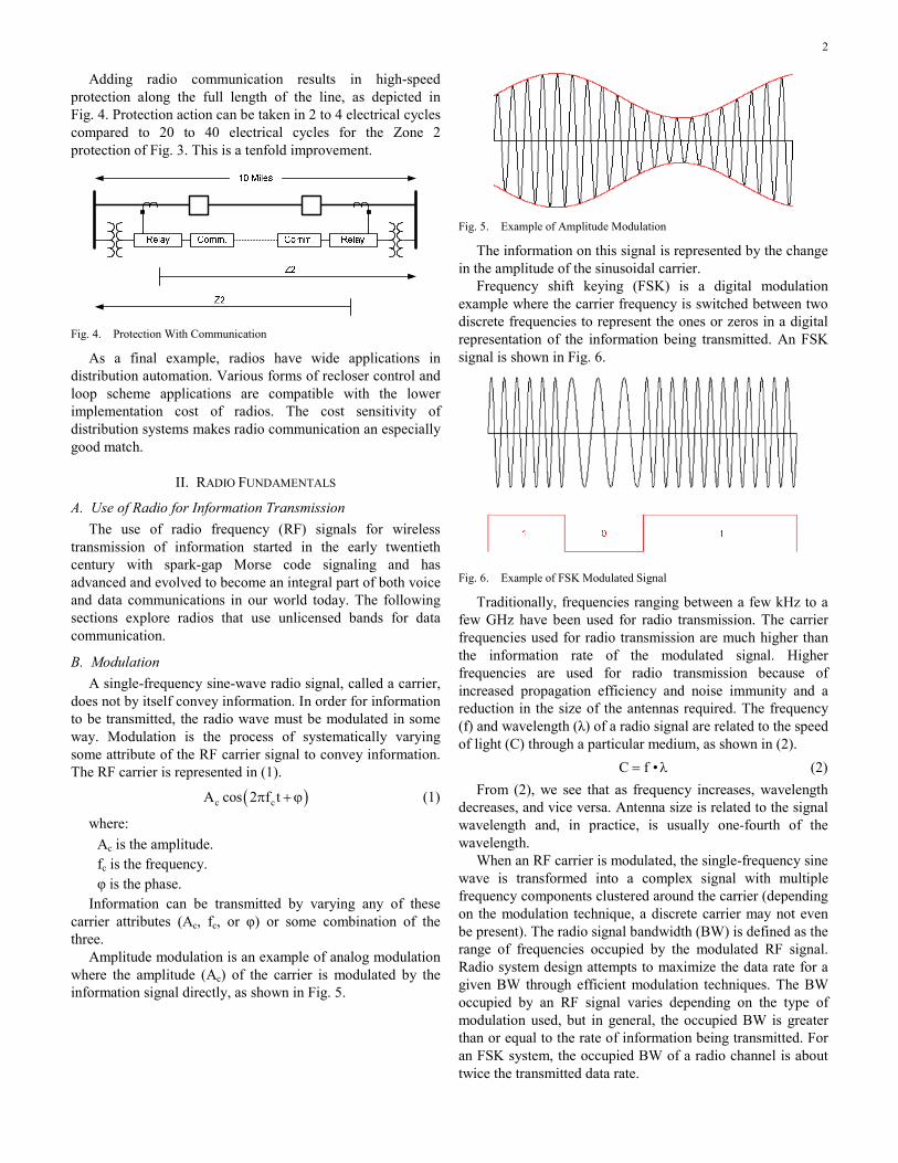
Amplitude modulation is an example of analog modulation where the amplitude (Ac) of the carrier is modulated by the information signal directly, as shown in Fig. 5.

Fig. 5. Example of Amplitude Modulation

The information on this signal is represented by the change in the amplitude of the sinusoidal carrier.

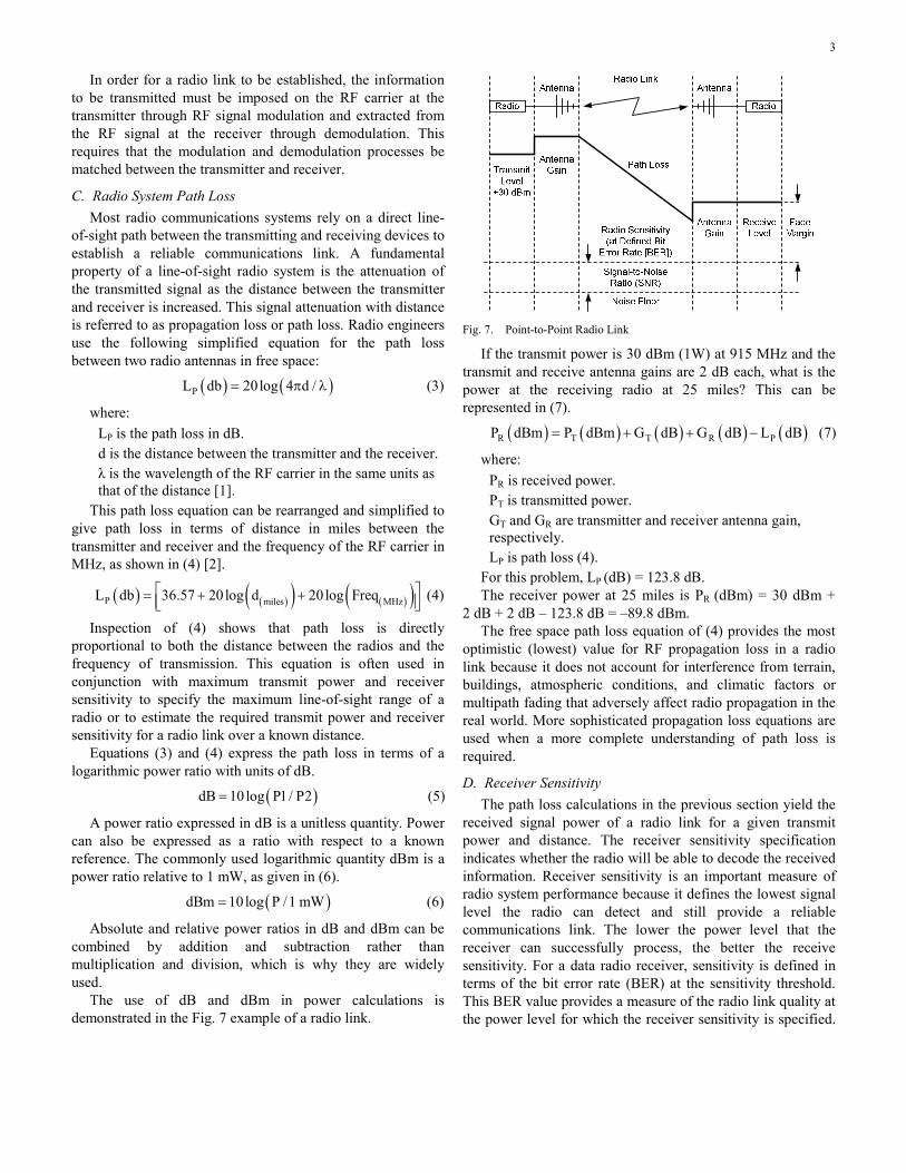
Frequency shift keying (FSK) is a digital modulation example where the carrier frequency is switched between two discrete frequencies to represent the ones or zeros in a digital representation of the information being transmitted. An FSK signal is shown in Fig. 6.

Fig. 6. Example of FSK Modulated Signal

Traditionally, frequencies ranging between a few kHz to a few GHz have been used for radio transmission. The carrier frequencies used for radio transmission are much higher than the information rate of the modulated signal. Higher frequencies are used for radio transmission because of increased propagation efficiency and noise immunity and a reduction in the size of the antennas required. The frequency (f) and wavelength (λ) of a radio signal are related to the speed of light (C) through a particular medium, as shown in (2). C f •= λ (2)

From (2), we see that as frequency increases, wavelength decreases, and vice versa. Antenna size is related to the signal wavelength and, in practice, is usually one-fourth of the wavelength.

When an RF carrier is modulated, the single-frequency sine wave is transformed into a complex signal with multiple frequency components clustered around the carrier (depending on the modulation technique, a discrete carrier may not even be present). The radio signal bandwidth (BW) is defined as the range of frequencies occupied by the modulated RF signal. Radio system design attempts to maximize the data rate for a given BW through efficient modulation techniques. The BW occupied by an RF signal varies depending on the type of modulation used, but in general, the occupied BW is greater than or equal to the rate of information being transmitted. For an FSK system, the occupied BW of a radio channel is about twice the transmitted data rate.

3

In order for a radio link to be established, the information to be transmitted must be imposed on the RF carrier at the transmitter through RF signal modulation and extracted from the RF signal at the receiver through demodulation. This requires that the modulation and demodulation processes be matched between the transmitter and receiver.

C. Radio System Path Loss Most radio communications systems rely on a direct line-

of-sight path between the transmitting and receiving devices to establish a reliable communications link. A fundamental property of a line-of-sight radio system is the attenuation of the transmitted signal as the distance between the transmitter and receiver is increased. This signal attenuation with distance is referred to as propagation loss or path loss. Radio engineers use the following simplified equation for the path loss between two radio antennas in free space:

( ) ( )PL db 20log 4 d /= π λ (3)

where: LP is the path loss in dB. d is the distance between the transmitter and the receiver. λ is the wavelength of the RF carrier in the same units as that of the distance [1].

This path loss equation can be rearranged and simplified to give path loss in terms of distance in miles between the transmitter and receiver and the frequency of the RF carrier in MHz, as shown in (4) [2].

( ) ( )( ) ( )( )P miles MHzL db 36.57 20log d 20log Freq⎡ ⎤= + +⎢ ⎥⎣ ⎦ (4)

Inspection of (4) shows that path loss is directly proportional to both the distance between the radios and the frequency of transmission. This equation is often used in conjunction with maximum transmit power and receiver sensitivity to specify the maximum line-of-sight range of a radio or to estimate the required transmit power and receiver sensitivity for a radio link over a known distance.

Equations (3) and (4) express the path loss in terms of a logarithmic power ratio with units of dB.

( )dB 10log P1/ P2= (5)

A power ratio expressed in dB is a unitless quantity. Power can also be expressed as a ratio with respect to a known reference. The commonly used logarithmic quantity dBm is a power ratio relative to 1 mW, as given in (6).

( )dBm 10log P /1 mW= (6)

Absolute and relative power ratios in dB and dBm can be combined by addition and subtraction rather than multiplication and division, which is why they are widely used.

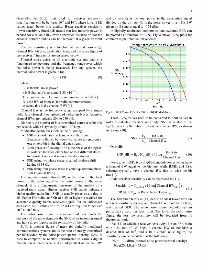
The use of dB and dBm in power calculations is demonstrated in the Fig. 7 example of a radio link.

Fig. 7. Point-to-Point Radio Link

If the transmit power is 30 dBm (1W) at 915 MHz and the transmit and receive antenna gains are 2 dB each, what is the power at the receiving radio at 25 miles? This can be represented in (7).

( ) ( ) ( ) ( ) ( )R T T R PP dBm P dBm G dB G dB L dB= + + − (7)

where: PR is received power. PT is transmitted power. GT and GR are transmitter and receiver antenna gain, respectively. LP is path loss (4).

For this problem, LP (dB) = 123.8 dB. The receiver power at 25 miles is PR (dBm) = 30 dBm +

2 dB + 2 dB – 123.8 dB = –89.8 dBm. The free space path loss equation of (4) provides the most

optimistic (lowest) value for RF propagation loss in a radio link because it does not account for interference from terrain, buildings, atmospheric conditions, and climatic factors or multipath fading that adversely affect radio propagation in the real world. More sophisticated propagation loss equations are used when a more complete understanding of path loss is required.

D. Receiver Sensitivity The path loss calculations in the previous section yield the

received signal power of a radio link for a given transmit power and distance. The receiver sensitivity specification indicates whether the radio will be able to decode the received information. Receiver sensitivity is an important measure of radio system performance because it defines the lowest signal level the radio can detect and still provide a reliable communications link. The lower the power level that the receiver can successfully process, the better the receive sensitivity. For a data radio receiver, sensitivity is defined in terms of the bit error rate (BER) at the sensitivity threshold. This BER value provides a measure of the radio link quality at the power level for which the receiver sensitivity is specified.

4

Generally, the BER limit used for receiver sensitivity specifications will be between 10–3 and 10–6, where lower BER values mean better link quality. Better receiver sensitivity (lower sensitivity threshold) means that less transmit power is needed for a reliable link over a specified distance or that the distance between radios can be increased at a given transmit power.

Receiver sensitivity is a function of thermal noise (PN), channel BW, bit rate, modulation type, and the noise figure of the receiver. These terms are discussed below.

Thermal noise exists in all electronic systems and is a function of temperature and the frequency range over which the noise power is being measured. For any system, the thermal noise power is given in (8). NP kTB= (8)

where: PN is thermal noise power. k is Boltzmann’s constant (1.38 • 10–23). T is temperature in kelvin (room temperature is 290°K). B is the BW of interest (for radio communications systems, this is the channel BW) [1].

Channel BW is the frequency range occupied by a single radio link channel. For unlicensed radios in North America, channel BWs are typically 200 to 250 kHz.

Bit rate is the number of bits transmitted across a radio link per second, which is typically around 100 Kbps.

Modulation techniques include the following: • FSK is a modulation scheme where the signal

frequency is flipped between two values to represent a one or zero bit in the digital data stream.

• With phase shift keying (PSK), the phase of the signal is switched between either two or four different states to represent ones and zeros in the data stream.

• PSK using two phase states is called bi-phase shift keying (BPSK).

• PSK using four phase states is called quadrature phase shift keying (QPSK).

The signal-to-noise ratio (SNR) is the ratio of the total power in the radio signal to the noise power in the radio channel. It is a fundamental measure of the quality of a received radio signal. Higher receiver SNR values indicate a higher-quality radio link. SNR is usually given as a value in dB. For an FM radio, an SNR of 6 dB or higher is required for acceptable quality in the received signal. For an unlicensed data radio, SNR values of 6 to 12 dB are required to achieve 10–3 to 10–6 BER.

The radio noise figure is a measure of how much the circuitry of the radio degrades the SNR of an incoming signal and has a direct impact on the sensitivity of the radio.

Eb/No is another figure of merit for digitally modulated communications systems and is the ratio of energy transmitted per bit divided by the noise power spectral density. Eb/No is used to compare the relative performance of various digital modulation schemes because it is independent of channel BW

and bit rate. Eb is the total power in the transmitted signal divided by the bit rate. No is the noise power in a 1 Hz BW given by (8) and is equal to –174 dBm.

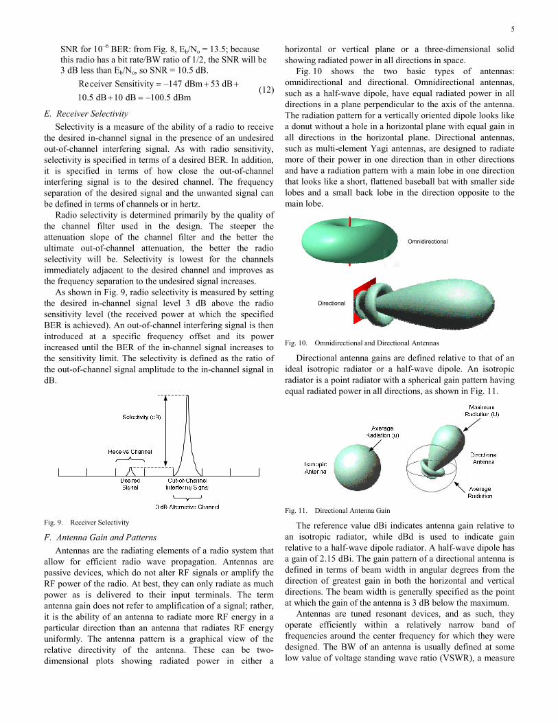
In digitally modulated communications systems, BER can be plotted as a function of Eb/No. Fig. 8 shows Eb/No plots for common digital modulation schemes.

Fig. 8. BER Versus Eb/No for FSK and BPSK Modulation

These Eb/No values need to be converted to SNR values in order to calculate receiver sensitivity. SNR is related to the Eb/No curves by the ratio of bit rate to channel BW, as shown in (9) and (10).

b

o

E Bit RateSNR •N Channel BW

= (9)

Or in dB:

( ) ( )b oBit RateSNR dB E / N dB 10log

Channel BW= + (10)

For a given BER, typical QPSK modulation schemes have a channel BW equal to the bit rate, while BPSK and FSK schemes typically have a channel BW that is twice the bit rate [1].

Radio receiver sensitivity can be expressed in (11).

( ) ( )( )( ) ( )

o dBm dB

dB dB

Sensitivity N 10log Channel BW

SNR @ BER Radio Noise Figure

= + +

+ (11)

The first three terms in (11) define an ideal lower limit on receiver sensitivity for a given channel BW, modulation type, and desired BER. The radio noise figure degrades system performance from this ideal limit. The lower the radio noise figure, the less the sensitivity will be degraded from its theoretical limit.

Use (11) to calculate receiver sensitivity. For an FSK radio with a bit rate of 100 kbps, a channel BW of 200 kHz, a desired BER of 10–6, and a 10 dB radio noise figure, the sensitivity can be calculated as the following:

No = –174 dBm (thermal noise power spectral density) 10log(200 kHz) = 53 dB

5

SNR for 10–6 BER: from Fig. 8, Eb/No = 13.5; because this radio has a bit rate/BW ratio of 1/2, the SNR will be 3 dB less than Eb/No, so SNR = 10.5 dB.

Receiver Sensitivity –147 dBm 53 dB10.5 dB 10 dB –100.5 dBm

= + ++ =

(12)

E. Receiver Selectivity Selectivity is a measure of the ability of a radio to receive

the desired in-channel signal in the presence of an undesired out-of-channel interfering signal. As with radio sensitivity, selectivity is specified in terms of a desired BER. In addition, it is specified in terms of how close the out-of-channel interfering signal is to the desired channel. The frequency separation of the desired signal and the unwanted signal can be defined in terms of channels or in hertz.

Radio selectivity is determined primarily by the quality of the channel filter used in the design. The steeper the attenuation slope of the channel filter and the better the ultimate out-of-channel attenuation, the better the radio selectivity will be. Selectivity is lowest for the channels immediately adjacent to the desired channel and improves as the frequency separation to the undesired signal increases.

As shown in Fig. 9, radio selectivity is measured by setting the desired in-channel signal level 3 dB above the radio sensitivity level (the received power at which the specified BER is achieved). An out-of-channel interfering signal is then introduced at a specific frequency offset and its power increased until the BER of the in-channel signal increases to the sensitivity limit. The selectivity is defined as the ratio of the out-of-channel signal amplitude to the in-channel signal in dB.

Fig. 9. Receiver Selectivity

F. Antenna Gain and Patterns Antennas are the radiating elements of a radio system that

allow for efficient radio wave propagation. Antennas are passive devices, which do not alter RF signals or amplify the RF power of the radio. At best, they can only radiate as much power as is delivered to their input terminals. The term antenna gain does not refer to amplification of a signal; rather, it is the ability of an antenna to radiate more RF energy in a particular direction than an antenna that radiates RF energy uniformly. The antenna pattern is a graphical view of the relative directivity of the antenna. These can be two-dimensional plots showing radiated power in either a

horizontal or vertical plane or a three-dimensional solid showing radiated power in all directions in space.

Fig. 10 shows the two basic types of antennas: omnidirectional and directional. Omnidirectional antennas, such as a half-wave dipole, have equal radiated power in all directions in a plane perpendicular to the axis of the antenna. The radiation pattern for a vertically oriented dipole looks like a donut without a hole in a horizontal plane with equal gain in all directions in the horizontal plane. Directional antennas, such as multi-element Yagi antennas, are designed to radiate more of their power in one direction than in other directions and have a radiation pattern with a main lobe in one direction that looks like a short, flattened baseball bat with smaller side lobes and a small back lobe in the direction opposite to the main lobe.

Omnidirectional

Directional

Fig. 10. Omnidirectional and Directional Antennas

Directional antenna gains are defined relative to that of an ideal isotropic radiator or a half-wave dipole. An isotropic radiator is a point radiator with a spherical gain pattern having equal radiated power in all directions, as shown in Fig. 11.

Fig. 11. Directional Antenna Gain

The reference value dBi indicates antenna gain relative to an isotropic radiator, while dBd is used to indicate gain relative to a half-wave dipole radiator. A half-wave dipole has a gain of 2.15 dBi. The gain pattern of a directional antenna is defined in terms of beam width in angular degrees from the direction of greatest gain in both the horizontal and vertical directions. The beam width is generally specified as the point at which the gain of the antenna is 3 dB below the maximum.

Antennas are tuned resonant devices, and as such, they operate efficiently within a relatively narrow band of frequencies around the center frequency for which they were designed. The BW of an antenna is usually defined at some low value of voltage standing wave ratio (VSWR), a measure

6

of reflected power, where the majority of the incident power is being radiated by the antenna. Typically, antennas have BWs on the order of 10 percent of their center frequency.

The radiation efficiency of an antenna depends on the impedance match between the transmission line connected to the antenna inputs and the antenna structure itself. Usually, a matching network is designed into the antenna input to achieve a good impedance match. Improper impedance matching adversely impacts the radiation efficiency and/or gain of the antenna. This loss of efficiency affects transmission and reception equally.

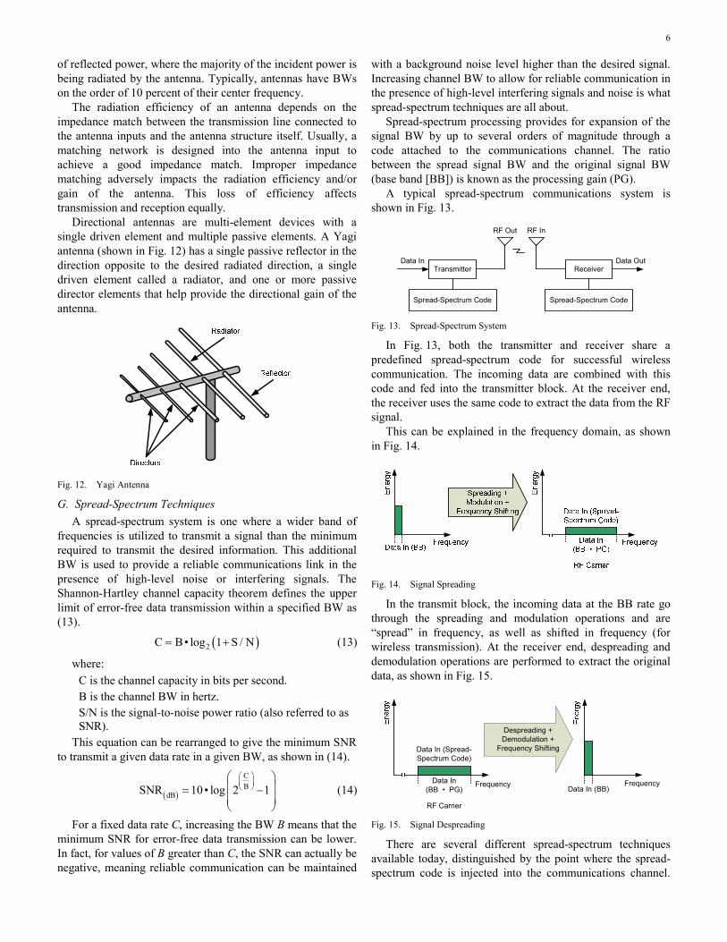
Directional antennas are multi-element devices with a single driven element and multiple passive elements. A Yagi antenna (shown in Fig. 12) has a single passive reflector in the direction opposite to the desired radiated direction, a single driven element called a radiator, and one or more passive director elements that help provide the directional gain of the antenna.

Fig. 12. Yagi Antenna

G. Spread-Spectrum Techniques A spread-spectrum system is one where a wider band of

frequencies is utilized to transmit a signal than the minimum required to transmit the desired information. This additional BW is used to provide a reliable communications link in the presence of high-level noise or interfering signals. The Shannon-Hartley channel capacity theorem defines the upper limit of error-free data transmission within a specified BW as (13).

( )2C B• log 1 S / N= + (13)

where: C is the channel capacity in bits per second. B is the channel BW in hertz. S/N is the signal-to-noise power ratio (also referred to as SNR).

This equation can be rearranged to give the minimum SNR to transmit a given data rate in a given BW, as shown in (14).

( )

CB

dBSNR 10• log 2 1⎛ ⎞⎜ ⎟⎝ ⎠

⎛ ⎞⎜ ⎟= −⎜ ⎟⎝ ⎠

(14)

For a fixed data rate C, increasing the BW B means that the minimum SNR for error-free data transmission can be lower. In fact, for values of B greater than C, the SNR can actually be negative, meaning reliable communication can be maintained

with a background noise level higher than the desired signal. Increasing channel BW to allow for reliable communication in the presence of high-level interfering signals and noise is what spread-spectrum techniques are all about.

Spread-spectrum processing provides for expansion of the signal BW by up to several orders of magnitude through a code attached to the communications channel. The ratio between the spread signal BW and the original signal BW (base band [BB]) is known as the processing gain (PG).

A typical spread-spectrum communications system is shown in Fig. 13.

Transmitter

Spread-Spectrum Code

Receiver

Spread-Spectrum Code

Data In Data Out

RF Out RF In

Fig. 13. Spread-Spectrum System

In Fig. 13, both the transmitter and receiver share a predefined spread-spectrum code for successful wireless communication. The incoming data are combined with this code and fed into the transmitter block. At the receiver end, the receiver uses the same code to extract the data from the RF signal.

This can be explained in the frequency domain, as shown in Fig. 14.

Fig. 14. Signal Spreading

In the transmit block, the incoming data at the BB rate go through the spreading and modulation operations and are “spread” in frequency, as well as shifted in frequency (for wireless transmission). At the receiver end, despreading and demodulation operations are performed to extract the original data, as shown in Fig. 15.

Despreading + Demodulation +

Frequency Shifting

FrequencyData In (BB • PG)

Data In (Spread-Spectrum Code)

RF Carrier

Data In (BB)Frequency

Fig. 15. Signal Despreading

There are several different spread-spectrum techniques available today, distinguished by the point where the spread-spectrum code is injected into the communications channel.

7

Two of the important techniques that are used in radios today are direct-sequence spread spectrum (DSSS) and frequency-hopping spread spectrum (FHSS).

In a DSSS radio, the spread-spectrum code is applied directly to the incoming data bits. The result of this is fed to the modulation and frequency shifter to generate the desired RF carrier for transmission. A DSSS system actually spreads the transmitted data across a wide BW by multiplying the data with a spreading code. This allows the DSSS system to provide immunity to noise, as well as interfering signals.

In an FHSS radio, the spread-spectrum code is applied to the RF carrier, which results in data transmission at various carrier frequencies as the carrier hops from frequency to frequency. In an FHSS system, the signal rapidly hops across multiple channels, which allows it to dodge a fixed interfering signal. Frequency spectra for DHSS and FHSS are shown in Fig. 16 and Fig. 17.

Fig. 16. DSSS Spectrum

Fig. 17. FHSS Spectrum

One of the several advantages of spread-spectrum technology includes resistance to interference and jamming. Intentional or unintentional jamming signals are rejected by the receiver because they do not contain the correct spread-spectrum key. This is illustrated in Fig. 18, which describes the DSSS system.

Fig. 18. DSSS Interference Processing Gain

In Fig. 18, the interfering signal is combined with the desired signal after the RF signal is transmitted out of the antenna. The interfering signal and the desired signals are received at the receiving end and go through the despreading and demodulation process. The desired signal is recovered, and the interfering signal is rejected because it does not have the correct key. The interfering signal is shown in the frequency domain before and after the despreading process to illustrate this process.

Both FHSS and DSSS are good at resisting interference from nearby radio transmitters. Because the frequencies are always changing for an FHSS system, it can dodge a jammer (a transmitter specifically designed to block radio transmissions on a given frequency). As illustrated before, a DSSS system avoids interference by diluting it using its spreading function. Spread-spectrum radios are good at avoiding common interference sources such as signals that stay in a narrow frequency band and do not move.

This is not the case when multiple spread-spectrum radios are operating in the same vicinity. For example, when more FHSS systems operate on the same frequency band, more systems are hopping to the same frequency simultaneously and garbling the data that must be transmitted at that frequency.

DSSS radios are good at resisting interference up to a certain point, but if the combined interference throughout the band rises to a certain level, the communication dramatically drops nearly to zero. For example, it takes only a small number of nearby FHSS systems to cripple a DSSS system. On the other hand, if a DSSS system is transmitting across the entire band, an FHSS system may be unable to find a clear channel to hop to. In summary, an FHSS system degrades more gracefully than DSSS, but both degrade in performance when operating near each other [3] [4].

H. Link Types (Point-to-Point, Point-to-Multipoint, and Repeater) Useful line-of-sight radio links can be established over a

wide range of distances, depending on radio capabilities and path suitability. Unlicensed radios are generally limited to distances on the order of 20 to 30 miles. These radio links can be configured in a number of ways, depending on the needs of the user.

A point-to-point system (shown in Fig. 19) consists of a pair of radios communicating only with each other to provide a communications link between specific nodes in a network. Point-to-point radio links commonly use directional antennas to maximize the signal strength between the two radios and to minimize interference from other sources.

Fig. 19. Point-to-Point Radio Link

8

A point-to-multipoint scheme involves a network of radios with a master (M) communicating with a number of remote sites (R1, R2, R3, and R4), as shown in Fig. 20. Point-to-multipoint schemes generally use an omnidirectional antenna for the master because of the need to broadcast the signal widely.

Fig. 20. Point-to-Multipoint Radio Link

A repeater uses multiple radios in a point-to-point scheme to establish a link where a single line-of-sight path is not viable. The repeater radios are set up at an intermediate point (or points) in the path between the ends of the link to relay the signals farther along to the opposite end of the link or to another repeater along the path. Repeaters are used where line of sight between the ends of the link is obscured or where the length of the path exceeds the range of a single pair of radios. This type of scheme is shown in Fig. 21 and uses directional antennas to maximize gain and minimize interference.

Fig. 21. Radio Repeater Link

III. SYSTEM PARAMETERS FOR POWER SYSTEM PROTECTION When applying radio technology in protection and control

applications, many factors play a large role in overall system performance and should be considered. Unlicensed radio systems have the advantage of costing much less than using fiber or pilot wires, but there are new challenges to making the radio channel meet the same requirements as cabled solutions. The following five items should be evaluated when selecting radios for protection and control applications:

• Latency • Availability • Security and dependability • Robustness in harsh environments • Encryption

A. Latency Minimizing the latency of the radio link is critical for high-

speed operations. Early radios for the control market did not suit these applications because the radios were designed for sending large amounts of data with buffering to overcome channel unavailability. This buffering caused large delays in operation and, in some instances, led to undesired operations. Newer radios now have operating modes that allow buffering to be turned off or have special operation modes to support specific protocols designed for control. Selection of protocol and radio latency, together, have a large effect on system performance and overall latency.

When using radio for a pilot protection scheme or for high-speed control, the maximum allowed radio latency varies from 1.5 to 2 cycles. When evaluating radio latency, it is important to know the minimum and maximum latency for a good radio link. Very popular spread-spectrum radios always have a variable latency and, depending on how the manufacturer designed the radio, will exhibit a small or large variability in latency. The latency, along with the availability of the link, provides the real average, minimum, and maximum latency expected for a given operation.

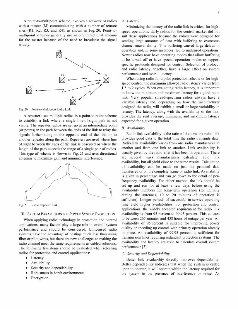
B. Availability Radio link availability is the ratio of the time the radio link

provides good data to the total time the radio transmits data. Radio link availability varies from one radio manufacturer to another and from one link to another. Link availability is usually given by the radio after it has been in operation. There are several ways manufacturers calculate radio link availability, but all yield close to the same results. Calculation of availability can be made on just the protocol data transferred or on the complete frame or radio link. Availability is given in percentage and can go down to the detail of per-frequency availability. For either method, the link should be set up and run for at least a few days before using the availability numbers for long-term operation (for initially aiming the antennas, 10 to 20 minutes of operation is sufficient). Longer periods of successful in-service operating time yield higher availabilities. For protection and control applications, the widely accepted requirement for radio link availability is from 95 percent to 99.95 percent. This equates to between 265 minutes and 438 hours of outage per year. An availability of 95 percent is suitable for improving power quality or speeding up control with primary operation already in place. An availability of 99.95 percent is sufficient for transmission lines requiring redundant protection systems. The availability and latency are used to calculate overall system performance [5].

C. Security and Dependability Better link availability directly improves dependability.

Better dependability indicates that when the system is called upon to operate, it will operate within the latency required for the system in the presence of interference or noise. As

9

availability decreases, dependability also decreases, so the system will not operate as needed. IEC 60834-1 references how to calculate and test the dependability and security of a system.

The security of a system is the ability of a link to properly operate when called upon and not operate when not called upon. Radio link security is highly dependent on the protocol used. Security is defined in IEC 60834-1 and can be calculated using (15).

uu

Err

NP

N≈ (15)

where: Pu is the probability of an unwanted command, and 1 – Pu is the security. Nu is the number of unwanted commands. NErr is the number of error bursts in the communications channel.

Radio link security is highly dependent on the protocol used and the error detection capabilities of the radio. The radio manufacturers should provide these numbers for specific radios and specific protocols [6].

D. Robustness in Harsh Environments Radio hardness and robustness are important for reliable

and dependable operation. The radio should meet the same type test standards and temperature requirements applied to relays. The scheme is only as good as the weakest link. Radios used in protection and control applications should meet or surpass the requirements of IEEE 1613, which lists all of the type tests needed to validate that a device is rugged enough to use for communication in electric power substations.

E. Encryption Providing a secure communications link that cannot be

compromised or manipulated by outsiders is important when using radio communication for sensitive information. Spread-spectrum and frequency-hopping techniques to some extent make it more difficult for an outsider to detect and decode a radio link, but they do not provide real data security. It is quite simple for someone using modern detection equipment to lock on to and decode either a DSSS or FHSS link. Encryption must be employed to provide data security.

Encryption is the process of using an algorithm, called a cipher, to transform user information into an unreadable form to prevent access and use of that information by anyone who does not possess the cipher key. Historically, encryption techniques have relied on substitution (substituting a different letter or block of letters of the alphabet for the original letter or block of letters with a substitution key available to the sender and receiver) and rearrangement, also known as permutation (rearrangement of letters in the original text according to a predefined key).

Modern electronic encryption algorithms continue to use these techniques in a much more sophisticated manner to provide cybersecurity for the power industry. The Advanced Encryption Standard (AES) encryption algorithm is widely

used today because of the security it provides and because it can be implemented efficiently in either hardware or software. This algorithm employs a symmetric key encryption standard with multiple transformation levels, each consisting of substitution and permutation processes, including one that relies on the encryption key. The algorithm operates on data blocks of 128 bits using a key of 128, 192, or 256 bits. This algorithm has been used by the United States government to protect data up to the top-secret level. The longer the key, the more levels of transformation are used in the algorithm and the more secure the encryption process will be.

Academic analysis (attack) of the AES algorithm has generated much debate about whether it can ultimately be broken, but leading experts do not believe that a practical method of intercepting AES encrypted data will ever be found. However, the ultimate weakness of any encryption scheme is user carelessness about security and access to the key. If hackers can obtain the key used in an encryption scheme, they have defeated the security as effectively as if they had broken the cipher itself and with infinitely less effort.

Secure, reliable, and dependable wireless systems require more initial work than wired systems. The IEEE 1613 and IEC 60834-1 standards still apply when using wireless links for communication and can help to guide the design of protection and control schemes. Working closely with manufacturers and using the available standards and information in radios help ensure acceptable radio system performance.

IV. RADIO APPLICATIONS

A. ITU Regions Radio regulations are determined on a country-by-country

basis. There is no overarching international body with legal authority. Instead, countries meet every four years in the World Radiocommunications Conference (WRC) organized by the International Telecommunications Union (ITU). These meetings produce recommendations that must be adopted by each country to have the effect of law. Some countries are close together or share common borders. Other countries are far from each other. To simplify the coordination, the ITU splits the world into three radio regions, as shown in Fig. 22. North and South America, including the Caribbean, are located in Radio Region 2.

Fig. 22. ITU World Radio Regions

10

B. Licensed Versus Unlicensed Radios All radio designs must be certified by the national body

before they can be used in a country. This is usually done by the manufacturer or by an importer for foreign-manufactured radios. To use a radio, a license is generally required; multiple radios may require multiple licenses.

There are a limited number of frequency bands that are unlicensed or lightly licensed. The most significant are the industrial, scientific, and medical (ISM) bands. In Radio Region 2, the best known ISM bands are the 915 MHz band, 2.4 GHz band (used for Wi-Fi®), and 5.8 GHz Unlicensed National Information Infrastructure (UNII) band. For communications applications, these bands generally use some form of spread-spectrum technology to limit the effects of interference.

C. FCC, IC, and COFETEL Inside the North American Free Trade Agreement

(NAFTA), each of the three countries has its own governmental body that regulates radio use. In Canada, it is Industry Canada (IC); in Mexico, it is the Comisión Federal de Telecomunicaciones (COFETEL); and in the United States, it is the Federal Communications Commission (FCC). These three bodies create regulations for different parts of the radio spectrum. The decisions are based on government decisions that balance national interests, consumer interests, international agreements (such as those in aviation), industry requirements, WRC recommendations, and cooperation with neighbors.

The most useful bands for electric protection systems and key subbands are described in Table I.

TABLE I IMPORTANT RADIO BANDS FOR UTILITY USE

Frequency Wavelength Band Description

30 to 300 MHz 10 to 1 m VHF Very high frequency.

300 to 3,000 MHz

1,000 to 100 mm UHF

Ultra high frequency. Various 400 MHz ISM bands

(RR1, RR3*). 868 short-range device (SRD)

bands (RR1, RR3*). 915 MHz ISM band (RR2*).

2.4 GHz ISM band. 3.65 GHz utility band (USA).

3 to 30 GHz 100 to 10 mm SHF Super high frequency.

5.8 UNII band. *RR1, RR2, and RR3 are ITU Radio Regions 1, 2, and 3.

D. Protection Engineer Perspective Not all radios can be used in all parts of the world.

Coordination by radio region provides some level of regional commonality. Cooperation between the United States and Canadian governments and increasing coordination with Mexico, due to NAFTA, are driving a growing set of product offerings that can be used across all three countries. A protection engineer working within a single country needs to

use the most appropriate band available in that country and make sure that radios are authorized for use in that country. Protection engineers working across country lines are still responsible to make sure individual radio types are approved in each country where they will be used. Using the same radios across NAFTA countries and nearby neighbors is becoming easier as cooperation between authorities increases.

V. SETTING UP RADIO LINKS There are many tools available to help set up a radio link

without a large initial investment and extensive knowledge about radios. The first step is a path study. Most radio manufacturers offer a free path study. This path study does not guarantee the link will work but helps to determine if the radio link is viable. Path study software uses terrain data, clutter data, radio-specific information, antenna design, and antenna tower height to calculate the path study. The terrain data include the elevations at different locations. The clutter data include an approximation of the vegetation height within defined regions. Most path studies do not take into account buildings or other man-made obstacles. These obstacles must be manually added to the path study.

The geographic information system (GIS) coordinates of an antenna tower and the maximum height of the mounted antennas are required inputs to the path study. The results of the study include the availability of the link and the link budget. Other inputs to a path study include radio hardware and antenna design details. The availability number given by the path study is an approximation of how well the link will work based upon propagation and multipath calculations. The initial target availability should ideally be greater than 99 percent. Again, this number is an approximation based upon the data entered, so actual results will vary.

The other important output of a path study is the fade margin. This is the difference between the received signal strength and the maximum sensitivity of the radio. To maintain a good link while minimizing radio interruptions, it is recommended to have at least 20 dB of margin. This margin decreases the likelihood that the received power level will degrade below the receiver sensitivity due to variable environmental effects, vegetation growth, or radio interference. Lower radio link margins will still work but can affect the long-term availability of the system.

An example of a link budget is shown in (16). T AT P AR F SP G L G M R+ + + − ≥ (16)

where: PT is transmit power. GAT is the transmitter antenna gain. LP is the path loss between the transmitter and receiver. GAR is the receiver antenna gain. MF is the fade margin. RS is the specified receiver sensitivity.

The inequality indicates that the sum of the elements on the left-hand side of the equation has to be greater than the radio receiver sensitivity in order to establish a reliable radio link.

11

A wide selection of antennas is available for ISM bands. Most manufacturers offer antennas that are best suited for the application and tested to meet FCC regulations. Most point-to-point links use high-gain Yagi antennas to transmit wireless information long distances over a narrow beam. Typical ISM band Yagi antennas have gains that range from 3 dB to 12 dB. A higher-gain antenna has a narrower beam and propagates the signal farther than a lower-gain antenna. Yagi antennas have gain on both transmitting and receiving sides. It is best to let the manufacturer choose the antenna based upon the path study. Other antennas may be used, but careful attention is needed to avoid violating regulations.

When setting up protection or control radio links, special care must be taken to ensure the reliability and dependability of communication beyond that required for supervisory control and data acquisition (SCADA) links. Choosing the right Yagi antenna and properly aiming the antenna are more critical in protection and control applications than when using radios for SCADA data collection. A Yagi antenna can be either vertically or horizontally polarized. The direction of polarization is the direction of the Efield radiated by the antenna.

Using oppositely polarized antennas on different radio links allows 20 dB of separation between signals on adjacent frequencies and helps reduce interference between radio links operating in close proximity to one another. Using the signal strength and availability is the key to creating a good radio link. The quickest way to commission a radio is to use the received signal strength indication (RSSI). The higher the RSSI value, the stronger the signal. Once both antennas are positioned with the highest RSSI, the radio link should be allowed to run for 10 or more minutes. After 10 minutes, the antennas should be aimed in different directions in 5-degree increments. When the measured availability is the highest at both ends, the antennas are aligned for the best performance. Any time the availability is less than 100 percent, there is either interference from environmental factors or other radios or multipath interference. Although directional antennas concentrate the majority of power from a radio transmitter along the line-of-sight path of the radio link, some of the signal can be scattered by objects (such as buildings, trees, and land cover). This scatter causes multiple images of the transmitted signal to reach the receiving antenna from more than one path. If these multipath signals sum out of phase with the desired signal, they can weaken the signal to the point that the receiver cannot detect it or will generate a high number of bit errors. When this happens, the radio error detection rejects the data. This is undesirable if a control signal must be sent at that instant of time. If the radio is set up for SCADA data use, the radio will detect the error and resend the message, and the end devices will never see the missing data. Aiming the antennas and minimizing multipath interference yields better dependability.

It can be desirable to set up multiple point-to-point links in substations requiring protection on each line. It is very convenient and inexpensive to set up multiple radio links with

multiple antennas located on the same antenna tower. This setup requires much more attention and careful antenna placement to approach the same performance levels as one dedicated point-to-point link. For example, for a pilot scheme using a radio link on each transmission line, it is easy to place three or more radio links at the substation to the other end of the line of a different substation. Ideally, it would be economical to place all three antennas on one pole. Placing multiple antennas on the same pole operating at the same frequency band can result in interference, with a significant impact on radio link performance. When one antenna at a shared site with multiple radio links is transmitting at 36 dBm and an adjacent antenna is trying to receive a signal from a remote location at –80 dBm, interference from the transmitting signal degrades receiver availability. The antenna transmitting at a high level overpowers the lower-level received signal from the remote location. There are several options to reduce the effect of interference between multiple radio links at a shared site, but these do not entirely eliminate the problem. Changing the polarization of the antennas provides a 20 dB improvement in isolation between a pair of radio links. For three antennas, increasing the separation between them will always help, as will reducing the transmit power. However, reducing the transmit power reduces availability, operating times, and dependability. One method to overcome this problem is to synchronize spread-spectrum radios at the shared location so they transmit and receive at exactly the same time. Radio synchronization reduces radio-to-radio interference to the level of difference in the received signals, which is generally less than 20 dB. Most radios on the market can properly reject adjacent signals at this level. Polarizing and moving the antennas farther apart will give even better results. Synchronizing the radios greatly improves availability and provides performance comparable to a single dedicated radio link.

VI. ECONOMIC BENEFITS The most basic electrical protection schemes operate

without the use of communication. Adding communication results in more accurate coverage and faster operation. Faster operation reduces stress on electrical components and improves overall power system stability and reliability. Better accuracy in coverage helps the protection scheme define where the event is located and reduces the probability of incorrect operation.

There are many different methods for providing communication in protection schemes. Often, a primary consideration is the communications system. A utility can lease communications or install their own. In the first case, the utility relinquishes some control and must pay monthly fees but does not have to make a capital investment in the communications infrastructure. For utility ownership, fiber-optic cable is the gold standard, but fiber is expensive. Hanging fiber-optic cable on poles is less expensive than burying fiber-optic cables. Rocky terrain and dense urban

12

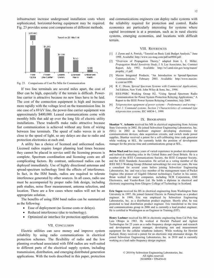
infrastructure increase underground installation costs where sophisticated, horizontal-boring equipment may be required. Fig. 23 provides some cost comparisons of different methods.

Fig. 23. Comparisons of Cost Per Mile for Communication

If two line terminals are several miles apart, the cost of fiber can be high, especially if the terrain is difficult. Power-line carrier is attractive because no new lines have to be laid. The cost of the connection equipment is high and increases more rapidly with the voltage level on the transmission line. In one case of a 69 kV line, the power-line carrier equipment was approximately $400,000. Leased communications come with monthly bills that add up over the long life of electric utility installations. These tradeoffs make radio attractive because fast communication is achieved without any form of wiring between line terminals. The speed of radio waves in air is close to the speed of light, so any delays are due to radio and protection electronics at each end.

A utility has a choice of licensed and unlicensed radios. Licensed radios require longer planning lead times because they cannot be placed in service until the licensing process is complete. Spectrum coordination and licensing costs are all complicating factors. By contrast, unlicensed radios can be deployed immediately. Use of highly directional antennas and spread-spectrum technology limit the effects of interference. In fact, in the ISM bands, radios are required to tolerate interference generated by other sources. In all cases, radio use must be accompanied by proper radio link design, including path studies, noise floor measurement, antenna selection, and location. There are a few cases where radios will not be an appropriate solution.

The benefits of using ISM band radios can be summarized as the following:

• Ease of deployment (no license costs or delays). • Reduced interference (due to technology). • Optimized air interface for protection applications.

VII. CONCLUSION Electric utilities can save money and improve system

reliability by using radio communications in electrical protection schemes. The flexibility of radio and the low planning overhead associated with ISM radios are well-suited to different parts of the electrical supply system, including transmission, distribution, and emerging distributed generation applications. With the tools described in this paper, protection

and communications engineers can deploy radio systems with the reliability required for protection and control. Radio economics are particularly interesting for systems where capital investment is at a premium, such as in rural electric systems, emerging economies, and locations with difficult terrain.

VIII. REFERENCES [1] J. Zyren and A. Petrick, “Tutorial on Basic Link Budget Analysis,” June

1998. Available: http://www.sss-mag.com/pdf/an9804.pdf. [2] “Overview of Propagation Theory,” adapted from L. E. Miller,

Propagation Model Sensitivity Study, J. S. Lee Associates, Inc. Contract Report, July 1992. Available: http://w3.antd.nist.gov/wctg/manet/ propthy_r1.pdf.

[3] Maxim Integrated Products, “An Introduction to Spread-Spectrum Communications,” February 2003. Available: http://www.maxim-ic.com/an1890.

[4] R. C. Dixon, Spread Spectrum Systems with Commercial Applications, 3rd Edition, New York: John Wiley & Sons, Inc., 1994.

[5] IEEE/PSRC Working Group H2, “Using Spread Spectrum Radio Communication for Power System Protection Relaying Applications,” A Report to the IEEE Power System Relaying Committee, July 2005.

[6] Teleprotection equipment of power systems – Performance and testing – Part 1: Command systems, Section 2 Characteristics of command type teleprotection systems, IEC 60834-1, 1999.

IX. BIOGRAPHIES Shankar V. Achanta received his MS in electrical engineering from Arizona State University in 2002. He joined Schweitzer Engineering Laboratories, Inc. (SEL) in 2002 as hardware engineer developing electronics for communications devices, data acquisition circuits, and switch mode power supplies. Shankar received a patent for a self-calibrating time code generator while working at SEL. He currently holds the position of development manager for the precise time and communications group at SEL.

Brian MacLeod has many years of varied experience in product development and technical marketing roles in the United States and Great Britain. He is a member of the IEEE Communications Society, the IEEE Computer Society, and the IEEE Standards Association. He served as a voting member of the IEEE 802.3 Working Group (Ethernet networking) for over ten years. He was a consultant for several years before joining Schweitzer Engineering Laboratories, Inc. and was a key member of the management team of Packet Engines (the pioneer of Gigabit Ethernet technology). Earlier in his career, Brian worked for major companies, including NCR Corporation, EMI Electronics, and Veeder-Root Ltd. He holds a diploma in electrical and electronic engineering from Glasgow College of Technology in Scotland.

Eric Sagen received his BS in electrical engineering from Washington State University in 1997. He joined General Electric in Pennsylvania as a product engineer. In 1999, Eric was employed by Schweitzer Engineering Laboratories, Inc. as a distribution product engineer. Shortly after, he was promoted to lead distribution product engineer. Eric transferred to the time and communications group in 2006 and is currently a lead product engineer. He is certified in Washington as an Engineer in Training (EIT).

Henry Loehner received his BS in electronic engineering from Cal Poly San Luis Obispo in 1983. He worked at Hewlett Packard and Agilent Technologies for 25 years as a radio frequency design engineer and research and development project manager, developing test and measurement equipment for the cellular telephone industry. While working for Hewlett Packard, Henry received a patent for an electronic step attenuator design. He joined Schweitzer Engineering Laboratories, Inc. in 2010 and is currently working as a lead radio frequency design engineer.

© 2010 by Schweitzer Engineering Laboratories, Inc. All rights reserved.

20100908 • TP6450-01