Applying Radar Cross-Section Estimations to Minimize Radar Echo

in Unmanned Combat Air Vehicle Design

Jillian G. Yuricich

2016

Thesis Committee:

Dr. Clifford Whitfield, Advisor

Dr. Richard Freuler

Department of Mechanical and Aerospace Engineering

Presented in Partial Fulfillment of the Requirements for Graduation with Honors Research

Distinction in Aeronautical and Astronautical Engineering at The Ohio State University

ii

Abstract

Radar profoundly altered the development of vehicle technology for combat especially in the realm of aircraft design. The technique of purpose-shaping an aircraft to minimize the vehicle’s radar cross-section and avoid detection on radar systems became a crucial step in the development of conceptual air vehicles, however much of this work is classified by the U.S. government. The purpose of this research is to develop the best methodology for predicting the radar cross-section of an aircraft throughout the design process by using open source radar equations. In order to estimate a radar cross-section value, simple shapes and their known radar cross-section expressions were used to represent all features of the conceptual aircraft design. An unmanned combat air vehicle designated the QF-36 Thunder was designed specifically for a radar-cross section analysis. Each of the QF-36’s main components, including wings, tails, and fuselage shape, were analyzed and their radar-cross section contribution calculated to ascertain the overall aircraft radar cross-section. Adjustments to specific aspects of the QF-36 could then be made to minimize the overall radar cross-section value while maintaining performance specifications set by the Request for Proposal which defined the vehicle’s mission. Following the development of this radar-cross section estimation tool, the results showed that large volume components including the fuselage and wing contributed the most to the total radar-cross section especially in the side- and front-view respectively. This trend aligns well with the initial idea of which aspects would contribute most to the radar-cross section. However, the main design advantage found throughout this process was that the tails contribute much less to the overall radar-cross section than initially hypothesized. This allows for large tails and better maneuverability with little increase in the overall radar echo. With this observation, design strategies may focus on minimizing wing size and maximizing tail size for the best compromise between radar-cross section minimization and enhanced performance. This research reflects one of few studies that documents the methodology for estimating radar cross-section of an aircraft in its entirety.

iii

Acknowledgements

First, I would like to dedicate this work to my parents and my sister without whom I would be lost. I also want to thank Dr. Clifford Whitfield for his guidance, encouragement, and general kindness throughout my time at Ohio State. He is a wonderful professor and person, and I am a better engineer because of him. I would also like to recognize the impression that Dr. Richard Freuler left on my life. He was the first professor I met at Ohio State, and our first meeting forever changed my college career. His mentorship has been one of the most valuable relationships I have made throughout my undergraduate experience. Finally, I would be remiss if I did not mention the wonderful friends I have made throughout my time at Ohio State in my Aeronautical and Astronautical Engineering courses. From late night study sessions around the dining room table to hours in the computer laboratory, we have been through so much together. I would not want to do it over again, but looking back, I would not change a thing. I love you all.

iv

Table of Contents

Abstract ....................................................................................................................................... ii

Acknowledgements .................................................................................................................... iii

Table of Contents ....................................................................................................................... iv

List of Figures ............................................................................................................................. v

List of Tables ............................................................................................................................. vi

Nomenclature ............................................................................................................................ vii

1. Introduction .......................................................................................................................... 1

1.1 The Radar Equation ...................................................................................................... 2

1.2 General Purpose-Shaping Knowledge .......................................................................... 4

2. Characteristic Wavelength Determination ........................................................................... 7

3. UCAV Development and Design....................................................................................... 13

3.1 Project Needs and Specifications Screening .............................................................. 13

3.2 Air Vehicle Configuration Options ............................................................................ 15

3.3 Final Configuration Selection ..................................................................................... 19

3.4 QF-36 Concept ........................................................................................................... 22

4. Radar-Cross Section Calculations...................................................................................... 23

4.1 UCAV Profile Selection ............................................................................................. 23

4.2 Front-View RCS Estimation ....................................................................................... 23

4.3 Side-View RCS Estimation ........................................................................................ 32

5. Discussion and Design Implications .................................................................................. 36

6. Conclusion ......................................................................................................................... 42

References ................................................................................................................................. 44

Appendix A: AIAA Request for Proposal .................................................................................. 1

Appendix B: QF-36 Concept Design Drawings ......................................................................... 1

Appendix C: Additional Information ......................................... Error! Bookmark not defined.

v

List of Figures

Figure 1: F-117A planform and faceted nose with radar reflection representation. ....................... 5 Figure 2: F-22 in formation flight with radar signal reflection. ...................................................... 6 Figure 3: Diagram of cylinders used to model a 95th-percentile male. ........................................ 10 Figure 4: UCAV screening chart. ................................................................................................. 14 Figure 5: Tailless aircraft with control-canard surface. ................................................................ 15 Figure 6: The B-2 bomber aircraft, an example of a tailless configuration. ................................. 16 Figure 7: Example of a tailless aircraft. ........................................................................................ 17 Figure 8: Delta wing configuration (A) and cranked arrow wing configuration (B). ................... 18 Figure 9: Conventional aircraft layout of the F-22 Raptor. .......................................................... 18 Figure 10: UCAV scoring chart. ................................................................................................... 21 Figure 11: QF-36 Thunder concept............................................................................................... 22 Figure 12: Front-view of UCAV................................................................................................... 23 Figure 13: Ogive and fuselage profile comparison with varying radii. ........................................ 25 Figure 14: Ogive and fuselage cross-section comparison with varying radii. .............................. 26 Figure 15: Ogive coordinate system and labels for side-view RCS estimation. ........................... 27 Figure 16: Side-view of UCAV .................................................................................................... 33 Figure 17: Flat plate RCS estimation with tail and wing front-view examples. ........................... 38

vi

List of Tables

Table 1: Radar cross-section estimations for various shapes at θ = 0o [4]. .................................... 3 Table 2: RCS values for various vehicles and objects. ................................................................... 7 Table 3: Anthropomorphic dimensions for 95th-percentile American male [12, 13]. .................... 9 Table 4: RCS distribution for each component of the 95th-percentile male figure. ........................ 9 Table 5: UCAV design criteria and requirements as set by AIAA RFP. ...................................... 13 Table 6: Front-view estimated values for forward fuselage. ........................................................ 28 Table 7: Front-view estimated values for tail surfaces. ................................................................ 29 Table 8: Front-view estimated values for wing surfaces. ............................................................. 30 Table 9: Front-view estimated values for the wing. ..................................................................... 31 Table 10: Front-view estimated values for the engine nacelles. ................................................... 32 Table 11: Total RCS of the QF-36 in the front-view. ................................................................... 32 Table 12: Side-view estimated values for the tail. ........................................................................ 33 Table 13: Fuselage represented by multiple spindles in the side view. ........................................ 34 Table 14: Total RCS for the QF-36 in the side-view. ................................................................... 35 Table 15: Various RCS estimations for past andpresent military aircraft and QF-36 concept. ... 36

vii

Nomenclature

AIAA American Institute of Aeronautics and Astronautics FLA Forward Looking Aft GHz Gigahertz (unit of electromagnetic wave equal to one billion hertz) HF High Frequency radar JSF Joint Strike Fighter (reference to the F-35 program) MEADS Medium Extended Air Defense System (radar system constructed by the

United States, Italy, and Germany) MHz Megahertz (unit of electromagnetic wave equal to one million hertz) OTH Over The Horizon radar system RFP Request for Proposal RCS Radar Cross-Section UCAV Unmanned Combat Aerial Vehicle UHF Ultra-High Frequency radar VHF Very High Frequency radar

1

1. Introduction

The use of radar in combat settings dramatically altered the course of vehicle technology in the

20th century. Introduced in World War II as a means of tracking enemy tanks, ships, and planes,

radar became an important investment for militaries globally. Radar operates by emitting radio

waves, or signals, delivered from a transmitter. If the radar signal contacts an object, the waves are

reflected back to a receiver. Using the speed of the waves and the time delay between transmission

and reception, the object’s distance from the radar source can be calculated. The magnitude of the

signal on the return transmission is also proportional to the size of the object detected. A larger

object has a larger radar echo, also known as and henceforth referred to as radar cross-section

(RCS) [1].

Radar was not without competition, however, and was countered with developments in stealth, or

low-observable, technologies. Within the last few decades, stealth characteristics have advanced

into one of the most critical aspects of military combat aircraft design [2]. These technologies aim

to increase air vehicle survivability by reducing the radar cross-section. While many technologies

such as radar-absorbing paint are included during the late stages of an air vehicle’s development

to reduce RCS, purpose-shaping is a method that can be applied from the inception of a new aircraft

design. Purpose-shaping techniques reduce the RCS by designing the geometry of the air vehicle’s

surface with the intention of reflecting radar waves away from the radar signal receiver [3].

This research investigated the use of equations for radar reflection and mathematical estimations

of simple shapes’ RCS values to determine a method for estimating the RCS of an air vehicle at a

single stage of the design process. This would allow the designer to better understand which

2

aspects of the vehicle design contribute the most toward the RCS in a quick, low-fidelity manner

as the design is manipulated to meet other performance parameters. The aircraft to be used in this

analysis is a design for an Unmanned Combat Aerial Vehicle (UCAV). The UCAV class of aircraft

will play a crucial role in the future of military aviation. With the current use of drone technology

in military reconnaissance, there will come a time where aviation technology in the military

matures enough for unmanned systems to be used in a fighter-combat role. This trend was seen

throughout World War I where once only used in reconnaissance missions, the maturation of

airplanes led to their use in combat in World War II opening up a new frontier of aviation. This

analysis of the UCAV is therefore very relevant to modern design studies.

1.1 The Radar Equation

Because existing approaches for calculating an aircraft’s exact RCS signature and size are

classified by the United States Department of Defense, this research will demonstrate the ability

to use open source equations to estimate an aircraft’s RCS value for use in conceptual design. It

was first necessary to understand the mathematical basis for radar and how it functions. The

fundamentals of radar can be observed within the radar equation which has been manipulated to

solve for range (𝑅𝑅):

𝑅𝑅 = �𝑃𝑃𝑡𝑡𝐺𝐺𝑡𝑡𝐺𝐺𝑟𝑟𝜎𝜎𝜆𝜆2

(4𝜋𝜋)3𝑃𝑃𝑟𝑟�1/4

(1)

where 𝑃𝑃𝑡𝑡 and 𝑃𝑃𝑟𝑟 (watts) are the transmitted power from the radar transmitter and receiver,

respectfully, 𝐺𝐺𝑡𝑡 and 𝐺𝐺𝑟𝑟 (unitless) are the gains of the transmitter and receiver, 𝜎𝜎 (square meters)

is the RCS and 𝜆𝜆 (meters) is the wavelength which can be calculated by:

3

𝜆𝜆 = 𝑐𝑐𝑓𝑓 (2)

where c, the speed of light, equals 3x108 (meters per second) and f is the radiated signal’s frequency

(Hertz). Since the 𝜎𝜎 (RCS) value only varies by the fourth root, only large changes in RCS value

will contribute to narrowing the range in which the aircraft would be detected [3]. However, once

in range, any amount of RCS reduction will help evade enemy detection.

With the RCS identified in the range equation, it was then important to understand how to quantify

a three-dimensional shape’s radar echo mathematically. These were the most useful equations for

this research. The main source of these RCS equations for simple shapes was a paper by Crispin

and Maffett [4]. This paper outlined the RCS calculations for generic spheroid shapes at various

angles of radar signal impingement. Spheroid have an RCS (σ) of:

𝜎𝜎 = 4𝜋𝜋𝑘𝑘4𝑉𝑉2 �1 + 1

𝜋𝜋𝜋𝜋𝑒𝑒−𝜋𝜋�

2 (3)

where y=b/a, V is volume, and k=2π/λ where λ is the wavelength of the emitted radar signal [4].

Manipulating this for specific spheroid shapes, the table below gives examples of equations used

to calculate the RCS (σ) given the shape’s geometric values. These equations are only valid at a

signal impingement angle of zero-degrees.

Table 1: Radar cross-section estimations for various shapes at θ = 0o [4].

Shape Geometry RCS Expression

Lens (revolved around y-axis)

𝑦𝑦 = 3𝑉𝑉

4𝜋𝜋𝑅𝑅3 sin3 𝜃𝜃

𝑉𝑉 = 2𝜋𝜋𝑅𝑅3

3(1 − cos𝜃𝜃)(1 − cos𝜃𝜃 + sin2 𝜃𝜃)

4

Elliptic Ogive

𝑦𝑦 = 3𝑉𝑉

4𝜋𝜋𝑏𝑏3(1− cos𝜃𝜃)3

𝑉𝑉 = 2𝜋𝜋𝜋𝜋𝑏𝑏2(sin𝜃𝜃 − 𝜃𝜃 cos𝜃𝜃 −13

sin3 𝜃𝜃)

Spindle (Paraboloid Ogive)

𝑦𝑦 =

4𝑐𝑐5𝑑𝑑

; 𝑉𝑉 =16𝜋𝜋𝑐𝑐𝑑𝑑2

15

Finite Cylinder Length = h, base radius = a 𝑦𝑦 =3ℎ4𝜋𝜋

; 𝑉𝑉 = 𝜋𝜋𝜋𝜋2ℎ

Cone-spheroid

𝑦𝑦 =ℎ + 2𝑏𝑏

4𝜋𝜋; 𝑉𝑉 =

𝜋𝜋𝜋𝜋2(ℎ + 2𝑏𝑏)3

Further information on the topic provided RCS equations for varying angles of radar signal

impingement for the spheroid as well as non-spheroid shapes including the cone, flat plate, and

very thin cylinder, or wire. These equations will be discussed at length when used.

1.2 General Purpose-Shaping Knowledge

As aforementioned, exact RCS calculations and techniques of purpose-shaping are classified, but

there is a wealth of general knowledge that exists regarding which shapes, surfaces, and aircraft

features contribute to an air vehicle’s RCS. A list of important features for designers to consider

include large components such as the wing and tail surfaces and their edges, the engine compressor

face, edges and flat sides to the air intakes, nozzle edges, and any 90-degree angles. It is also

known that external fuel tanks, pods, and stores, the cockpit instrumentation, and pilot helmet

contribute to a higher RCS. The UCAV already has an advantage here. Because this is an

unmanned vehicle, there will be no cockpit in this design, and therefore no cockpit let alone

instrumentation or helmet. However, other internal components on all aircraft give off their own

5

radar signals, including an altimeter, range seeker, GPS, and other avionic devices. Unfortunately,

these will also contribute to an increased RCS [10].

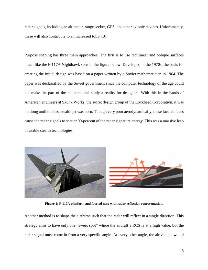
Purpose shaping has three main approaches. The first is to use rectilinear and oblique surfaces

much like the F-117A Nighthawk seen in the figure below. Developed in the 1970s, the basis for

creating the initial design was based on a paper written by a Soviet mathematician in 1964. The

paper was declassified by the Soviet government since the computer technology of the age could

not make the part of the mathematical study a reality for designers. With this in the hands of

American engineers at Skunk Works, the secret design group of the Lockheed Corporation, it was

not long until the first stealth jet was born. Though very poor aerodynamically, these faceted faces

cause the radar signals to scatter 99-percent of the radar signature energy. This was a massive leap

in usable stealth technologies.

Another method is to shape the airframe such that the radar will reflect in a single direction. This

strategy aims to have only one “sweet spot” where the aircraft’s RCS is at a high value, but the

radar signal must come in from a very specific angle. At every other angle, the air vehicle would

Figure 1: F-117A planform and faceted nose with radar reflection representation.

6

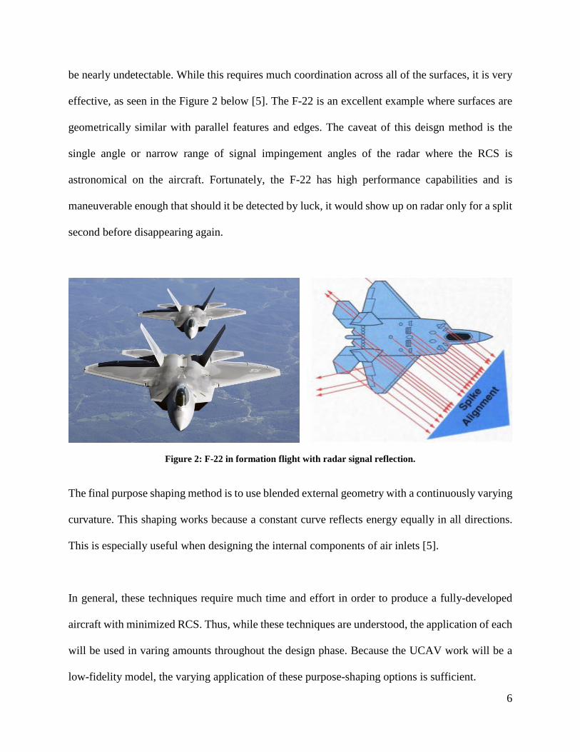
be nearly undetectable. While this requires much coordination across all of the surfaces, it is very

effective, as seen in the Figure 2 below [5]. The F-22 is an excellent example where surfaces are

geometrically similar with parallel features and edges. The caveat of this deisgn method is the

single angle or narrow range of signal impingement angles of the radar where the RCS is

astronomical on the aircraft. Fortunately, the F-22 has high performance capabilities and is

maneuverable enough that should it be detected by luck, it would show up on radar only for a split

second before disappearing again.

The final purpose shaping method is to use blended external geometry with a continuously varying

curvature. This shaping works because a constant curve reflects energy equally in all directions.

This is especially useful when designing the internal components of air inlets [5].

In general, these techniques require much time and effort in order to produce a fully-developed

aircraft with minimized RCS. Thus, while these techniques are understood, the application of each

will be used in varing amounts throughout the design phase. Because the UCAV work will be a

low-fidelity model, the varying application of these purpose-shaping options is sufficient.

Figure 2: F-22 in formation flight with radar signal reflection.

7

2. Characteristic Wavelength Determination

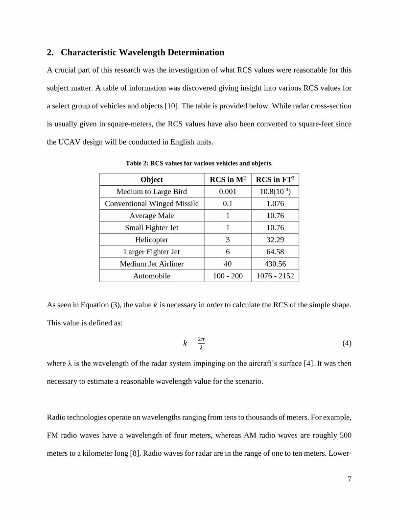
A crucial part of this research was the investigation of what RCS values were reasonable for this

subject matter. A table of information was discovered giving insight into various RCS values for

a select group of vehicles and objects [10]. The table is provided below. While radar cross-section

is usually given in square-meters, the RCS values have also been converted to square-feet since

the UCAV design will be conducted in English units.

Table 2: RCS values for various vehicles and objects.

Object RCS in M2 RCS in FT2 Medium to Large Bird 0.001 10.8(10-4)

Conventional Winged Missile 0.1 1.076 Average Male 1 10.76

Small Fighter Jet 1 10.76 Helicopter 3 32.29

Larger Fighter Jet 6 64.58 Medium Jet Airliner 40 430.56

Automobile 100 - 200 1076 - 2152

As seen in Equation (3), the value 𝑘𝑘 is necessary in order to calculate the RCS of the simple shape.

This value is defined as:

𝑘𝑘 = 2𝜋𝜋𝜆𝜆

(4)

where λ is the wavelength of the radar system impinging on the aircraft’s surface [4]. It was then

necessary to estimate a reasonable wavelength value for the scenario.

Radio technologies operate on wavelengths ranging from tens to thousands of meters. For example,

FM radio waves have a wavelength of four meters, whereas AM radio waves are roughly 500

meters to a kilometer long [8]. Radio waves for radar are in the range of one to ten meters. Lower-

8

frequency radar is very effective against stealth vehicles, and for radar frequencies less than 900

MHz, the RCS of the target vehicle increases exponentially regardless of any stealth geometry

profile. This means that radar for use in detection and tracking, the system must strike a balance

between a well-defined RCS signal and the ability to detect and differentiate between any object

flying overhead. Low-frequency radar was used in Kosovo to track and shoot down the first stealth

jet, the F-117 Nighthawk [9]. Currently, A- and B-band, or High Frequency (HF) and Very-High

Frequency (VHF), radar systems range 300 MHz and below and have long been used as early

warning and Over The Horizon (OTH) systems. However, these systems are limited by the size of

their physical subsystems including antennas. Because of this limitation, C-Band, or Ultra-High

Frequency (UHF), radar systems which range in operation from 300 MHz to 1 GHz are productive

for detection and tracking of satellites and missiles over a long range especially for early warning

and target acquisition missions [11]. An example of such a system is the Medium Extended Air

Defense System (MEADS) which is an international program between the United States, German,

and Italian militaries.

With this information, it was then possible to make an estimation of wavelength and check to see

how reasonable the value is based on known information regarding radar systems. Because no

declassified information exists on what radar frequencies or wavelengths are used in military radar

systems, the human male example from Table 2 was used to determine a useful wavelength and,

therefore, a 𝑘𝑘 value. The profile of a human was replicated using the finite cylinder shape from

Crispin and Maffett’s paper as seen in Table 1. Cylinders of various dimensions represented the

legs, torso with arms, and head of a 95th-percentile male. The 95th-percentile was chosen because

a larger human would drive a higher RCS. Based on the equations from Crispin and Maffett, this

9

contributes to a lower wavelength necessary to achieve the intended RCS. A lower wavelength

will in turn drive the aircraft RCS higher, which will overestimate the UCAV’s RCS. Therefore,

the RCS estimations are worst case scenario. The dimensions of the 95th-percentile male can be

seen below.

Table 3: Anthropomorphic dimensions for 95th-percentile American male [12, 13].

Feature Dimension Bitragion Breadth (Head Width) 6.1 IN

Menton to top of head (Head Height) 9.1 IN Head length (Head Depth) 8.2 IN

Shoulder (bideltoid) breadth (Torso Width) 21.1 IN Mid-shoulder height, sitting (Torso Height) 26.7 IN

Torso Depth 6.4 IN Leg Width (Torso Width) 21.1 IN

Crotch Length (Leg Height) 36.1 IN Leg Depth 4.2 IN

After each portion of the male figure was represented by a Crispin/Maffett cylinder, the RCS was

calculated. The key aspect of this study involved the adjustment of the wavelength until the RCS

total of the human reached the desired 10.76 square-feet (1 m2) from Table 2. A table of each

component’s corresponding contribution to the overall RCS is included. The distribution of

cylinders used to model the male subject can be seen below as well.

Table 4: RCS distribution for each component of the 95th-percentile male figure.

Component RCS Value in M2 RCS Value in FT2 Head 0.00382 0.0411

Torso and Arms 0.4324 4.6522 Legs 0.5638 6.0660

Total 1 10.7593

10

Figure 3: Diagram of cylinders used to model a 95th-percentile male.

The corresponding wavelength for a human male RCS of 10.76 square-feet (1 m2) was 6.8996 feet

(2.1030 m2). As seen in the following equation, for a constant wave velocity, the frequency is

inversely proportional to the wavelength.

𝑓𝑓 = 𝑣𝑣𝜆𝜆 (5)

With the determined wavelength of 6.9 feet, or 2.103 meters, and a wave velocity at the speed of

light, 3(108) m/s, the frequency would be roughly 142 GHz. This estimate reflects the use of High-

Frequency (HF) or A-Band radar as the radar system used to track this aircraft. While the frequency

is lower than most declassified types of radar known today, this lower band of frequency is being

revived in the world of radar technology due to the advancements within the electronics field,

especially in micronization of modern technology [11]. The estimation of wavelength, while lower

than conventional systems of today, proves to be a great example of what future radar technologies

may use to track and detect aerial targets.

Head

Torso

Leg

Wavelength

11

It is important to understand that modern radar systems do operate at much higher frequencies and

therefore shorter wavelengths for systems in place in hostile territory for close-range monitoring.

However, at shorter wavelengths, the RCS is much smaller. Therefore, the wavelength chosen for

this research can be considered as a worst case scenario. It is quite possible that systems operating

in hostile territory would not use A-band radar below 900 MHz, which would be a distinct

advantage to any stealth aircraft.

Overall, the 6.8996-foot wavelength from the human RCS investigation is a reasonable estimate

wavelength when using Crispin and Maffett’s equations. This wavelength estimate will be kept

constant for the entire process of estimating RCS and provides a value of 𝑘𝑘 from Equation (4). The

calculation is as follows:

𝑘𝑘 =2𝜋𝜋𝜆𝜆

=2𝜋𝜋6.9

= 0.9106

The RCS estimation of each component is calculated as follows using Equation (3) and the now

known value of 𝑘𝑘.

𝜎𝜎 = 4𝜋𝜋

(0.9106)4𝑉𝑉2 �1 +1𝜋𝜋𝑦𝑦

𝑒𝑒−𝜋𝜋�2

𝜎𝜎 = (0.8755)𝑉𝑉2 �1 + 1𝜋𝜋𝜋𝜋𝑒𝑒−𝜋𝜋�

2 (6)

Equation (7) has been simplified to include the constant value of 𝑘𝑘. Each component of the aircraft

will individually contribute a specific 𝑉𝑉 and 𝑦𝑦 value to fill the remaining variables of the equation.

It is important to note that Crispin and Maffett also provided equations that do not use the RCS

Equation (7) from above. Other variations of these equations exist for the same shapes, and they

take into account the angle at which the radar signal is impinging on the simple shape from zero

12

to 90-degrees. These equations can be helpful for features of the aircraft that do not lie parallel to

the lateral, longitudinal, or vertical planes where the signal’s angle of impingement is neither zero

nor 90-degrees.

13

3. UCAV Development and Design

3.1 Project Needs and Specifications Screening The UCAV design originated from an American Institute of Aeronautics and Astronautics (AIAA)

Request for Proposal (RFP) for an undergraduate student design competition. The following table

describes the criteria and requirements for the UCAV as set by the AIAA RFP. As well, the full

RFP document can be found in Appendix A: AIAA Request for Proposal.

Table 5: UCAV design criteria and requirements as set by AIAA RFP.

Criteria Requirement Cruise Ceiling 60000 FT Runway Length 10000 FT Payload (expendable) 4100 LBS Range (unrefueled) 2000 NM at M 1.6 Cruise Mach 1.5 Dash Mach 2.0 Time to Accelerate from M 0.93 to M 2 at 50000 ft. 2 MIN (maximum)

NRE $10 billion Flyaway Cost $200 million for 200 aircraft buy

The most important requirements set by the RFP were that the vehicle be unmanned, semi-

autonomous, and combat capable with high performance. It was then added for the purposes of

this research that the UCAV be designed with the minimization of the RCS in mind.

The UCAV was screened in order to better understand which requirements were the most critical

to the design. The scoring chart is as follows:

14

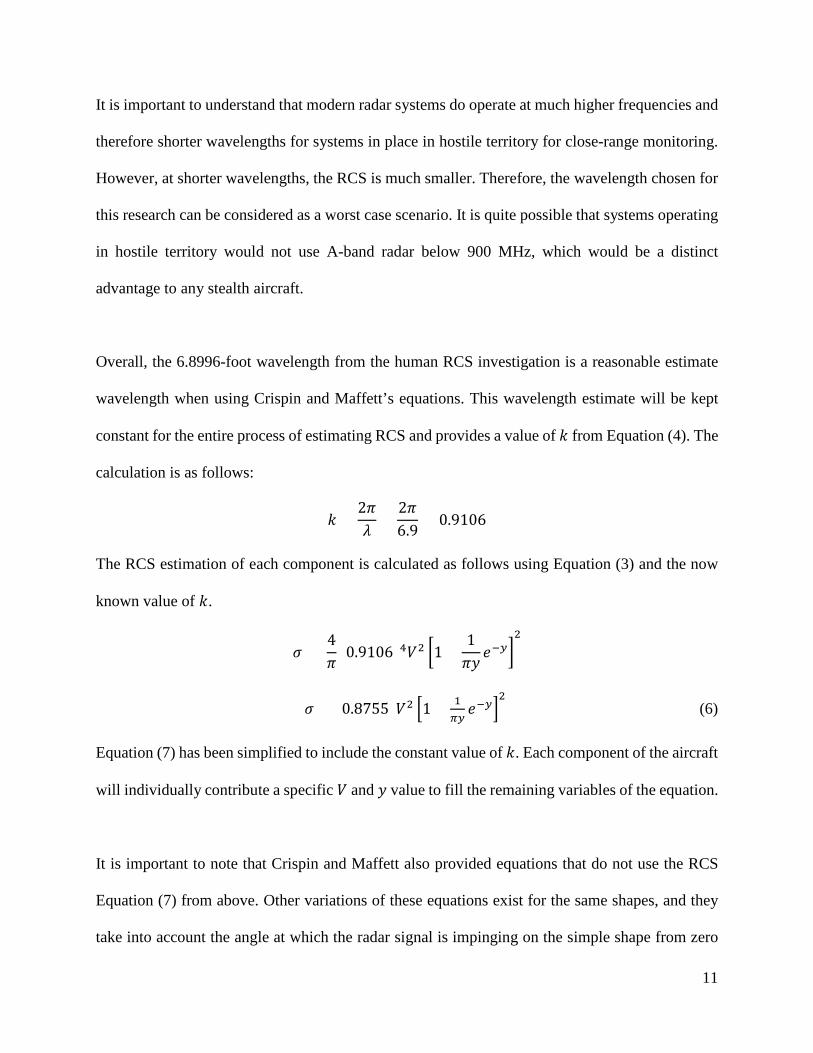
Figure 4: UCAV screening chart.

The results from this chart show that critical factors include cost specifications, time to accelerate,

the 180-degree turn with weapons, the load factors of +12/-8G, and the cruise and dash Mach

values. While some of these, especially cost, were predictable, it is helpful to narrow down the

most important parts of the UCAV’s mission so that they can be taken into careful consideration

during the preliminary design process. It is clear that a large power plant will be necessary to meet

the speed requirements as well as a strong and robust structure to handle high loads. As well, the

design will have to be aerodynamically efficient to ensure that range is met at the high speeds

required.

15

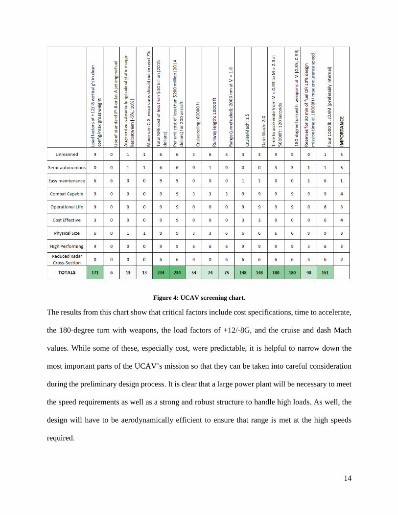
3.2 Air Vehicle Configuration Options From here, configuration options were weighed. It was narrowed immediately to six layout

options: tailless, control-canard, flying wing, delta wing, cranked arrow and conventional

configurations. An example of a tailless aircraft, sometimes coupled to include the control-canard,

can be seen below.

Figure 5: Tailless aircraft with control-canard surface.

The control-canard was the first to be analyzed. For some designs, aircraft with control-canard can

have high maneuverability due to the inherent destabilization of the aircraft by the canards. A

control-canard can also counteract pitch-up moments due to tip stall by having significant nose-

down deflection. This fact can be used to optimize the wing’s aspect ratio and wing sweep. Close

coupling to the wing also allows for directed airflow over the wings at high angles of attack to

provide more lift, reduce drag, and delay stall. These attributes are especially helpful in supersonic

delta wing configurations in transonic and low-speed flight regimes such as landing and takeoff.

However, the use of a control-canard does come at some cost. The large, angular surface can have

a negative impact on stealth characteristics due to the tendency to reflect large amounts of radar

signals forward. There can also be adverse flow disturbances from the canard over the wing. After

this investigation, it was clear that a control-canard could be a viable option to supplement any

larger wing or fuselage design [6].

16

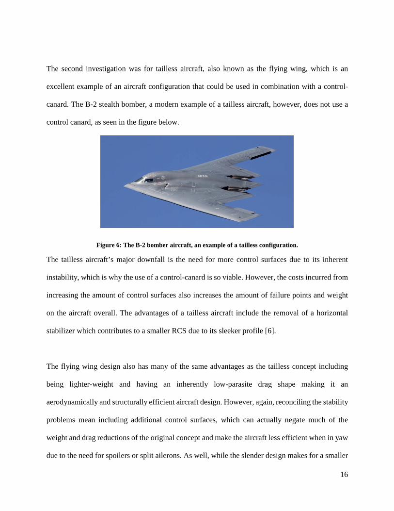
The second investigation was for tailless aircraft, also known as the flying wing, which is an

excellent example of an aircraft configuration that could be used in combination with a control-

canard. The B-2 stealth bomber, a modern example of a tailless aircraft, however, does not use a

control canard, as seen in the figure below.

Figure 6: The B-2 bomber aircraft, an example of a tailless configuration.

The tailless aircraft’s major downfall is the need for more control surfaces due to its inherent

instability, which is why the use of a control-canard is so viable. However, the costs incurred from

increasing the amount of control surfaces also increases the amount of failure points and weight

on the aircraft overall. The advantages of a tailless aircraft include the removal of a horizontal

stabilizer which contributes to a smaller RCS due to its sleeker profile [6].

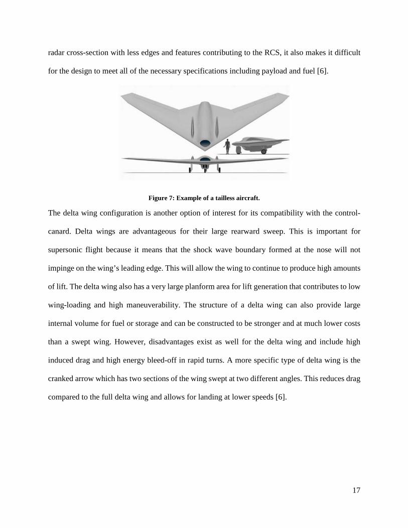
The flying wing design also has many of the same advantages as the tailless concept including

being lighter-weight and having an inherently low-parasite drag shape making it an

aerodynamically and structurally efficient aircraft design. However, again, reconciling the stability

problems mean including additional control surfaces, which can actually negate much of the

weight and drag reductions of the original concept and make the aircraft less efficient when in yaw

due to the need for spoilers or split ailerons. As well, while the slender design makes for a smaller

17

radar cross-section with less edges and features contributing to the RCS, it also makes it difficult

for the design to meet all of the necessary specifications including payload and fuel [6].

Figure 7: Example of a tailless aircraft.

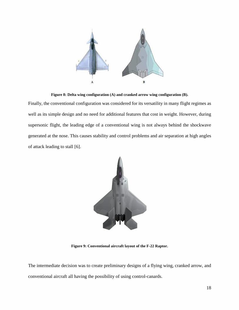
The delta wing configuration is another option of interest for its compatibility with the control-

canard. Delta wings are advantageous for their large rearward sweep. This is important for

supersonic flight because it means that the shock wave boundary formed at the nose will not

impinge on the wing’s leading edge. This will allow the wing to continue to produce high amounts

of lift. The delta wing also has a very large planform area for lift generation that contributes to low

wing-loading and high maneuverability. The structure of a delta wing can also provide large

internal volume for fuel or storage and can be constructed to be stronger and at much lower costs

than a swept wing. However, disadvantages exist as well for the delta wing and include high

induced drag and high energy bleed-off in rapid turns. A more specific type of delta wing is the

cranked arrow which has two sections of the wing swept at two different angles. This reduces drag

compared to the full delta wing and allows for landing at lower speeds [6].

18

Figure 8: Delta wing configuration (A) and cranked arrow wing configuration (B).

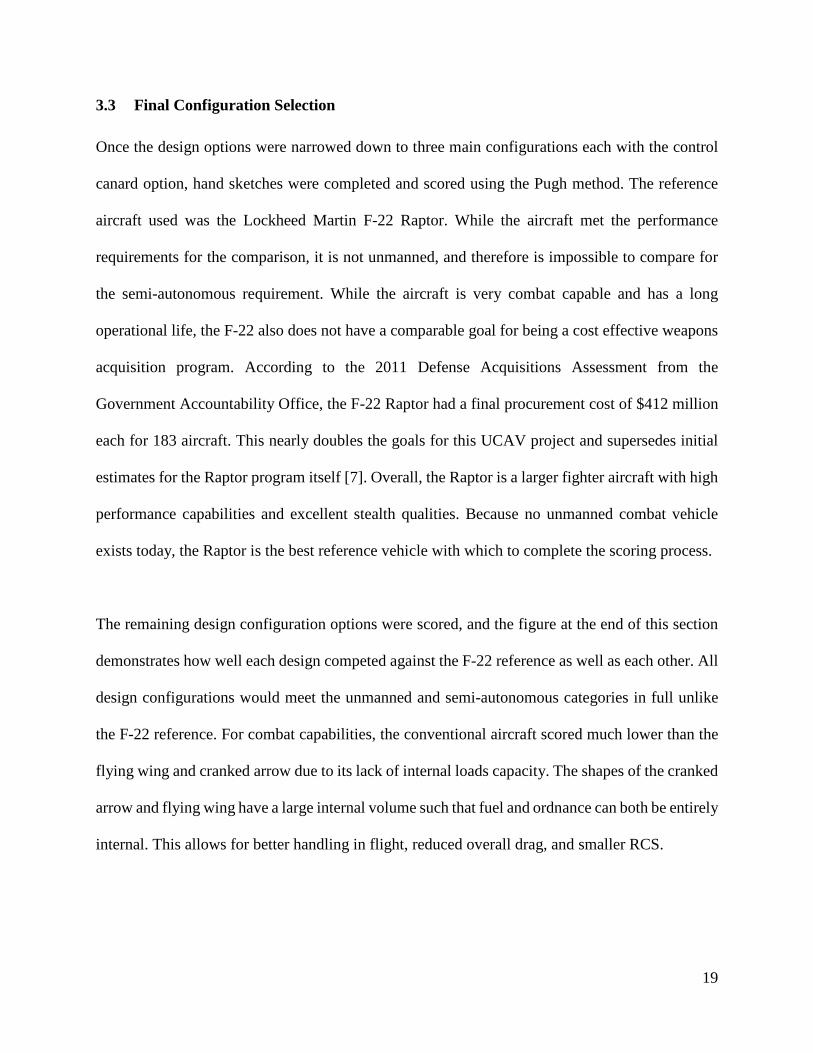
Finally, the conventional configuration was considered for its versatility in many flight regimes as

well as its simple design and no need for additional features that cost in weight. However, during

supersonic flight, the leading edge of a conventional wing is not always behind the shockwave

generated at the nose. This causes stability and control problems and air separation at high angles

of attack leading to stall [6].

Figure 9: Conventional aircraft layout of the F-22 Raptor.

The intermediate decision was to create preliminary designs of a flying wing, cranked arrow, and

conventional aircraft all having the possibility of using control-canards.

19

3.3 Final Configuration Selection Once the design options were narrowed down to three main configurations each with the control

canard option, hand sketches were completed and scored using the Pugh method. The reference

aircraft used was the Lockheed Martin F-22 Raptor. While the aircraft met the performance

requirements for the comparison, it is not unmanned, and therefore is impossible to compare for

the semi-autonomous requirement. While the aircraft is very combat capable and has a long

operational life, the F-22 also does not have a comparable goal for being a cost effective weapons

acquisition program. According to the 2011 Defense Acquisitions Assessment from the

Government Accountability Office, the F-22 Raptor had a final procurement cost of $412 million

each for 183 aircraft. This nearly doubles the goals for this UCAV project and supersedes initial

estimates for the Raptor program itself [7]. Overall, the Raptor is a larger fighter aircraft with high

performance capabilities and excellent stealth qualities. Because no unmanned combat vehicle

exists today, the Raptor is the best reference vehicle with which to complete the scoring process.

The remaining design configuration options were scored, and the figure at the end of this section

demonstrates how well each design competed against the F-22 reference as well as each other. All

design configurations would meet the unmanned and semi-autonomous categories in full unlike

the F-22 reference. For combat capabilities, the conventional aircraft scored much lower than the

flying wing and cranked arrow due to its lack of internal loads capacity. The shapes of the cranked

arrow and flying wing have a large internal volume such that fuel and ordnance can both be entirely

internal. This allows for better handling in flight, reduced overall drag, and smaller RCS.

20

As for operational life, all aircraft scored equally since each configuration would be designed to

be easily maintainable and structurally sound. However, the configurations varied in scoring for

cost effectiveness. Because the flying wing has not been tested as extensively in supersonic flight,

it would take more research and development to build the knowledge base and technology for the

flying wing to be effective at those high speeds. On the contrary, the conventional and cranked

arrow configurations have both been heavily studied for supersonic flight and would require less

research and development investment.

The physical size of the aircraft configurations was also considered. Because supersonic flight

requires more purpose-shaping using the ideal Sears-Haack body as a reference, the flying wing

suffered in this category. This is due to the fact that a flying wing would need to be very large in

order to be effective at supersonic speeds. The conventional and cranked arrow configurations,

however, would be more compact while still being effective at supersonic speeds.

The performance aspect was also rated for each configuration. Again, the flying wing was rated

quite a bit lower relative to the other two configurations because of its lack of control authority.

While all of the designs may be inherently unstable for combat-performance purposes, the flying

wing has less control surfaces to exert control over the aircraft while maneuvering. This means

that the flying wing is not as agile an option as the cranked arrow and conventional crafts.

Finally, the radar cross-section was rated for each of the aircraft configurations. Because radar

cross-section reducing technologies exist in many forms from radar-absorbing paint to low-

probability-of-intercept radar on-board the vehicle, each aircraft was rated close to each other in

21

value. The shaping of the aircraft greatly impacts the vehicles observability on enemy radars, and

therefore distinctions between the three were made. The conventional configuration simply does

not fare well in this category due to its protruding wing and stabilizer surfaces. However, since the

flying wing design has a smooth and blended fuselage shape, it has the lowest radar cross-section

of the three designs. The cranked arrow is somewhere between the two others.

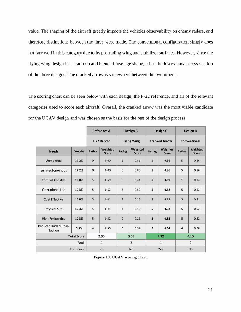
The scoring chart can be seen below with each design, the F-22 reference, and all of the relevant

categories used to score each aircraft. Overall, the cranked arrow was the most viable candidate

for the UCAV design and was chosen as the basis for the rest of the design process.

Reference A Design B Design C Design D

F-22 Raptor Flying Wing Cranked Arrow Conventional

Needs Weight Rating Weighted Score Rating Weighted

Score Rating Weighted Score Rating Weighted

Score

Unmanned 17.2% 0 0.00 5 0.86 5 0.86 5 0.86

Semi-autonomous 17.2% 0 0.00 5 0.86 5 0.86 5 0.86

Combat Capable 13.8% 5 0.69 3 0.41 5 0.69 1 0.14

Operational Life 10.3% 5 0.52 5 0.52 5 0.52 5 0.52

Cost Effective 13.8% 3 0.41 2 0.28 3 0.41 3 0.41

Physical Size 10.3% 5 0.41 1 0.10 5 0.52 5 0.52

High Performing 10.3% 5 0.52 2 0.21 5 0.52 5 0.52

Reduced Radar Cross-Section

6.9% 4 0.39 5 0.34 5 0.34 4 0.28

Total Score 2.90 3.59 4.72 4.10

Rank 4 3 1 2

Continue? No No Yes No

Figure 10: UCAV scoring chart.

22

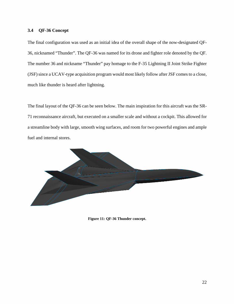
3.4 QF-36 Concept The final configuration was used as an initial idea of the overall shape of the now-designated QF-

36, nicknamed “Thunder”. The QF-36 was named for its drone and fighter role denoted by the QF.

The number 36 and nickname “Thunder” pay homage to the F-35 Lightning II Joint Strike Fighter

(JSF) since a UCAV-type acquisition program would most likely follow after JSF comes to a close,

much like thunder is heard after lightning.

The final layout of the QF-36 can be seen below. The main inspiration for this aircraft was the SR-

71 reconnaissance aircraft, but executed on a smaller scale and without a cockpit. This allowed for

a streamline body with large, smooth wing surfaces, and room for two powerful engines and ample

fuel and internal stores.

Figure 11: QF-36 Thunder concept.

23

4. Radar-Cross Section Calculations

4.1 UCAV Profile Selection In order to remain within the timeframe of completion for this research, the UCAV was to be

analyzed from two angles, or views. The first was the head-on view, or front-view. This was

selected for the front view’s relevance when approaching hostile territory. As the UCAV

approaches the enemy, the radar systems would detect the UCAV from the front looking aft (FLA).

This scenario is one of the most typical that a combat aircraft would face when deployed. The

second view chosen for analysis was the side-view. If the UCAV would have a mission to fly

parallel along enemy territory, the side-view would be detected from the perspective of the enemy

radar. It is therefore important that for both of these views, the RCS be minimized so as to evade

detection from the enemy for as long as possible. The bottom view of the aircraft was not chosen

for analysis due to the short time period that the underside of the vehicle would be visible by enemy

radar directed upward. By the time the vehicle would be detected and its presence understood, the

UCAV would have completed its mission and evacuated the territory.

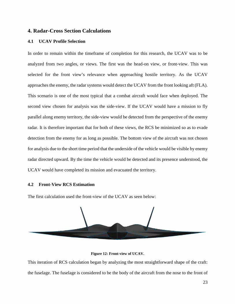
4.2 Front-View RCS Estimation The first calculation used the front-view of the UCAV as seen below:

Figure 12: Front-view of UCAV.

This iteration of RCS calculation began by analyzing the most straightforward shape of the craft:

the fuselage. The fuselage is considered to be the body of the aircraft from the nose to the front of

24

engine inlets which is more easily seen in Figure 11. The shape chosen for this fuselage was the

lens, or ogive.

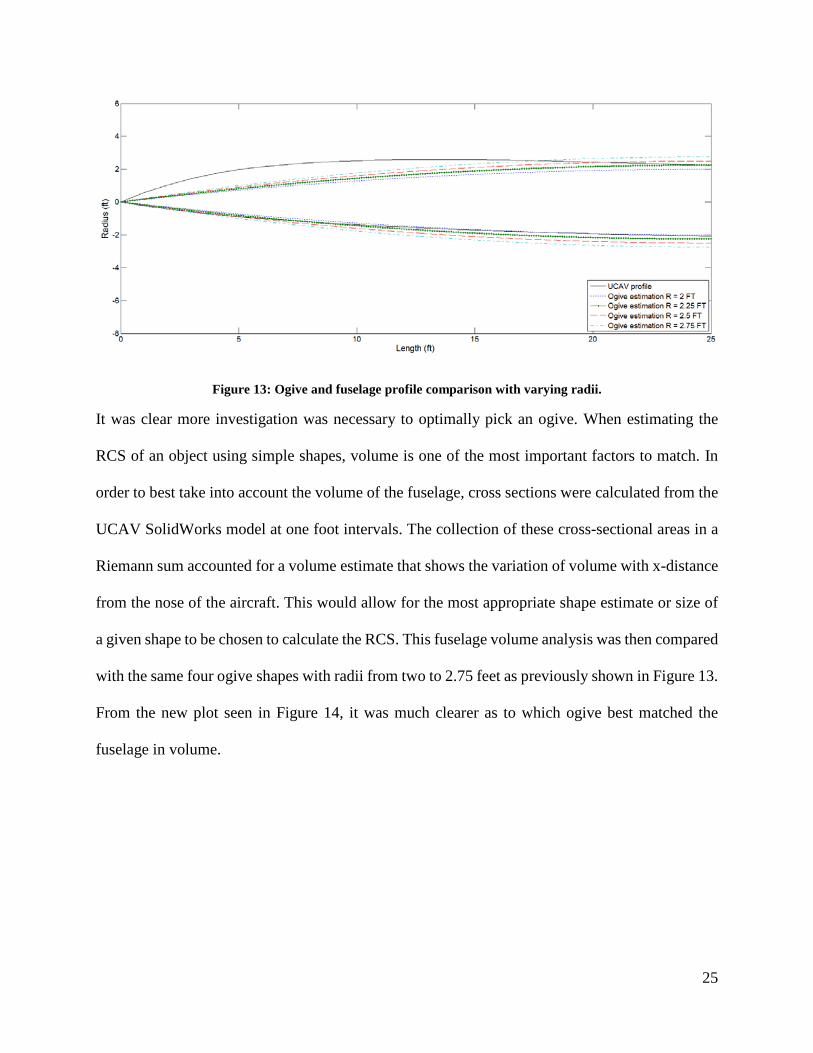
Once the ogive shape was selected, it was necessary to match the correct size to the profile and

shape of the UCAV fuselage. First, an equation for the ogive was found to plot its profile in the

X-Y plane as a means of comparison to the fuselage shape. The equation for an ogive is given as:

𝑦𝑦 = �𝜌𝜌2 − (𝐿𝐿 − 𝑥𝑥)2 + 𝑅𝑅 − 𝜌𝜌 (7)

For this shape, ρ is the radius of the larger circle that makes up the profile edge of the lens. It is

expressed as:

𝜌𝜌 = 𝑅𝑅2+𝐿𝐿2

2𝑅𝑅 (8)

The length of the fuselage is 25 feet up to the engine inlets, and therefore 𝐿𝐿 was set as a constant

of 25. The remaining variable was 𝑅𝑅 was varied to compare to the size and shape of the actual

UCAV fuselage design. The closest values of 𝑅𝑅 that nearly met the shape of the UCAV were

between two and 2.75 feet. The plot in Figure 13 is of the actual profile of the fuselage and ogive

shapes. The profile from zero to ten feet is not exactly met by the ogive estimation, however, as

the fuselage lengthens, the ogive shape better matches the profile. Based on radii variations alone,

it is unclear from Figure 13 as to which ogive shape best meets the fuselage shape.

25

Figure 13: Ogive and fuselage profile comparison with varying radii.

It was clear more investigation was necessary to optimally pick an ogive. When estimating the

RCS of an object using simple shapes, volume is one of the most important factors to match. In

order to best take into account the volume of the fuselage, cross sections were calculated from the

UCAV SolidWorks model at one foot intervals. The collection of these cross-sectional areas in a

Riemann sum accounted for a volume estimate that shows the variation of volume with x-distance

from the nose of the aircraft. This would allow for the most appropriate shape estimate or size of

a given shape to be chosen to calculate the RCS. This fuselage volume analysis was then compared

with the same four ogive shapes with radii from two to 2.75 feet as previously shown in Figure 13.

From the new plot seen in Figure 14, it was much clearer as to which ogive best matched the

fuselage in volume.

26

Figure 14: Ogive and fuselage cross-section comparison with varying radii.

The fuselage was best represented by the ogive with a radius of 2.5 feet. While the ogive cross-

sectional area is slightly below the fuselage from zero to 14 feet, it makes up for the losses from

14 to 25 feet. The estimation was then sufficient enough to predict the RCS contribution from the

fuselage.

The aforementioned work is proof that the ogive is an excellent shape to be used when estimating

the forward fuselage. However, new equations, variables, and coordinate systems are used to

calculate the ogive RCS. All of these equations share similar names and variables, however, the

following calculations refer to the labels in the Figure 15.

27

Figure 15: Ogive coordinate system and labels for side-view RCS estimation.

Unlike the ogive-lens estimation from Table 1, this new coordinate system seen in Figure 15 relies

on a different equation to estimate the shape’s RCS. Equation (10) is true for varying values of

theta from zero to (90 − 𝛼𝛼) degrees.

𝜎𝜎 = (𝑅𝑅1𝑎𝑎)𝜆𝜆2 tan4 𝛼𝛼16𝜋𝜋 cos6 𝜃𝜃(1−tan2 𝛼𝛼 tan2 𝜃𝜃)3 (9)

Because theta is equal to zero for the fuselage in the front-view, Equation (10) can be reduced to

following:

𝜎𝜎 = (𝑅𝑅1𝑎𝑎)𝜆𝜆2 tan4 𝛼𝛼16𝜋𝜋

(10)

An important change has been made to the previous two equations that was not reflected in the

study by Crispin and Maffett. These equations provided in the Crispin/Maffett study did not have

the correct units of RCS in the report and, after much deliberation, were adjusted to include the

sizing parameters of the width and radius. The product of these two parameters were multiplied to

the numerator of Equation (10) in order to reflect the correct units of RCS. This decision was made

based on other equations provided within the same report.

28

With this new expression, an RCS value for the fuselage was calculated using the following

defined variables including the wavelength estimated earlier to be 6.9 feet. As well, using the top

view of the aircraft, alpha (𝛼𝛼) can be measured to be 13.69°. Using Equation (13) and the known

values of the wavelength and alpha (𝛼𝛼), the RCS contribution from the forward fuselage can be

calculated and seen in Table 6 below.

Table 6: Front-view estimated values for forward fuselage.

Variable Value 𝜆𝜆 6.8996 [FT] 𝑅𝑅1 105.67 [FT] 𝜋𝜋 3.00 [FT] 𝛼𝛼 13.69°

𝝈𝝈 1.0570 [FT2] 0.982 [M2]

The next calculations were those of the tails. The flat plate is an adequate shape for modeling

leading edges of wing and fin surfaces and represents the surface as a collection or summation of

thin wires [4]. The equation for a square flat plate is as follows:

𝜎𝜎 = 4𝜋𝜋𝑎𝑎4

𝜆𝜆2�sin(𝑘𝑘𝑎𝑎 sin𝜃𝜃)

𝑘𝑘𝑎𝑎 sin𝜃𝜃�2 (11)

For the flat plate, the coordinate plane is set such that when the radar is impinging the plate

perpendicular to its surface, theta is equal to zero. Therefore, at the edge of the plate, radar is

impinging the surface at a theta equal to 90-degrees. Since the tails are mounted parallel to the

fuselage nose such that in the front view, theta is equal to 90-degrees, the flat plate equation can

be further simplified.

𝜎𝜎 = 4𝜋𝜋𝑎𝑎4

𝜆𝜆2�sin(𝑘𝑘𝑎𝑎 sin𝜃𝜃)

𝑘𝑘𝑎𝑎 sin𝜃𝜃�2

= 4𝜋𝜋𝑎𝑎4

𝜆𝜆2�sin(𝑘𝑘𝑎𝑎)

𝑘𝑘𝑎𝑎�2 (12)

29

This equation refers to both wavelength (𝜆𝜆) and 𝑘𝑘 as solved for previously. As well, Equation (14)

includes the value 𝜋𝜋, which refers to the characteristic side length of the square plate. Again, the

role of similar volume and area is taken into account when using the dimensions of the tail. The

tail area is 57.97 square feet, and therefore a square of side length 7.6138 has the equivalent area.

This will be used as the representative side length for the tail RCS estimation.

Table 7: Front-view estimated values for tail surfaces.

Variable Value 𝜆𝜆 6.8996 [FT] 𝑘𝑘 0.6767 [FT-1]

𝜋𝜋𝑡𝑡𝑎𝑎𝑖𝑖𝑖𝑖 7.7440 [FT]

𝝈𝝈 0.2877 [FT2]

Therefore, using the previous information and characteristic lengths calculated, each tail’s RCS

contribution is equal to 0.1592 square feet.

Aft of the fuselage nose is the blended wing-body. In order to estimate these components together

in the front view, the lens shape was used for its similarity to the wing profile from the FLA. This

entailed the use of the ogive again as was done for the fuselage nose.

From the previous estimation, Equation (10) was used because it was accurate near low values of

theta. However, as seen in Figure 15, theta was no longer equal to zero. Using the assigned

coordinate system, the value of theta was 90-degrees since the radar was impinging from the side.

This entailed using a new equation for the ogive RCS estimation. According to Crispin and

Maffett, the equation valid near theta values of 90-degrees is as follows:

30

𝜎𝜎 = 𝜋𝜋𝑅𝑅12 �1 −𝑅𝑅1−𝑎𝑎𝑅𝑅1 sin𝜃𝜃

� (13)

Since theta was equal to 90-degrees, and the equation reduced as follows:

𝜎𝜎(𝜃𝜃) = 𝜋𝜋𝑅𝑅12 �1 −𝑅𝑅1 − 𝛼𝛼𝑅𝑅1 sin𝜃𝜃

� = 𝜋𝜋𝑅𝑅12 �1 −𝑅𝑅1 − 𝛼𝛼𝑅𝑅1

� = 𝜋𝜋𝛼𝛼𝑅𝑅1

The CAD drawing provided the measurements needed to calculate the estimated RCS. The ogive

shape was estimated to best fit the curvature of the underside of the UCAV. This resulted in an

alpha (α) value equal to 8.5°. This did not match the top of the UCAV shape as well, but it was an

acceptable compromise considering future plans for estimating the engine nacelles. The table of

values and final RCS estimation for the wing-body using the ogive to calculate RCS can be seen

below:

Table 8: Front-view estimated values for wing surfaces.

Variable Value 𝜃𝜃 90° α 8.91° 𝑅𝑅1 3222.99 [FT] 𝜋𝜋 3.89 [FT]

𝝈𝝈 1975.5864 [FT2] 183.605 [M2]

From these estimations, it is clear that the use of the ogive to estimate the wing-body as a whole

is not appropriate. Other alternatives in estimations include the lens and the cone spheroid,

however, upon further investigation, these simple shapes were also a poor estimation of the wing-

body portion of the UCAV and grossly overestimated the wing-body RCS even more so than the

ogive. It was therefore necessary to divide the wing-body into more simple shapes for estimation.

31

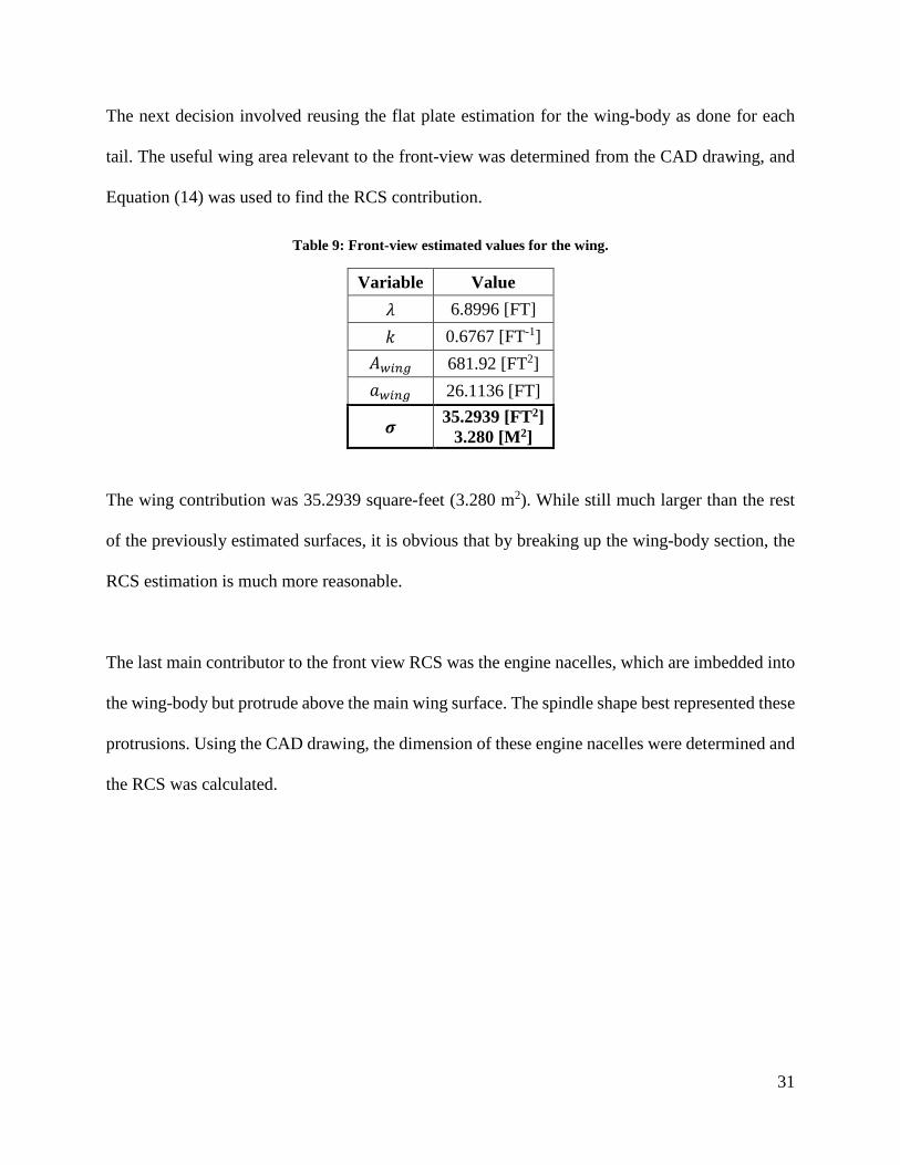
The next decision involved reusing the flat plate estimation for the wing-body as done for each

tail. The useful wing area relevant to the front-view was determined from the CAD drawing, and

Equation (14) was used to find the RCS contribution.

Table 9: Front-view estimated values for the wing.

Variable Value 𝜆𝜆 6.8996 [FT] 𝑘𝑘 0.6767 [FT-1]

𝐴𝐴𝑤𝑤𝑖𝑖𝑤𝑤𝑤𝑤 681.92 [FT2] 𝜋𝜋𝑤𝑤𝑖𝑖𝑤𝑤𝑤𝑤 26.1136 [FT]

𝝈𝝈 35.2939 [FT2] 3.280 [M2]

The wing contribution was 35.2939 square-feet (3.280 m2). While still much larger than the rest

of the previously estimated surfaces, it is obvious that by breaking up the wing-body section, the

RCS estimation is much more reasonable.

The last main contributor to the front view RCS was the engine nacelles, which are imbedded into

the wing-body but protrude above the main wing surface. The spindle shape best represented these

protrusions. Using the CAD drawing, the dimension of these engine nacelles were determined and

the RCS was calculated.

32

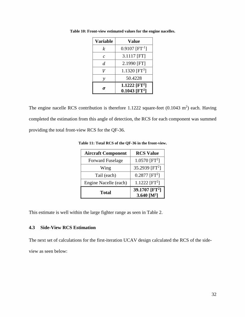
Table 10: Front-view estimated values for the engine nacelles.

Variable Value 𝑘𝑘 0.9107 [FT-1] 𝑐𝑐 3.1117 [FT] 𝑑𝑑 2.1990 [FT] 𝑉𝑉 1.1320 [FT3] 𝑦𝑦 50.4228

𝝈𝝈 1.1222 [FT2] 0.1043 [FT2]

The engine nacelle RCS contribution is therefore 1.1222 square-feet (0.1043 m2) each. Having

completed the estimation from this angle of detection, the RCS for each component was summed

providing the total front-view RCS for the QF-36.

Table 11: Total RCS of the QF-36 in the front-view.

Aircraft Component RCS Value Forward Fuselage 1.0570 [FT2]

Wing 35.2939 [FT2] Tail (each) 0.2877 [FT2]

Engine Nacelle (each) 1.1222 [FT2]

Total 39.1707 [FT2] 3.640 [M2]

This estimate is well within the large fighter range as seen in Table 2.

4.3 Side-View RCS Estimation The next set of calculations for the first-iteration UCAV design calculated the RCS of the side-

view as seen below:

33

Figure 16: Side-view of UCAV

By returning to the flat plate theory for the tails, the same Equation (13) was used with a new value

of theta. The tails are offset at an angle of 18.43-degrees outward which changes the value of theta

in Equation (13); the simplified Equation (14) is no longer valid for this scenario. Therefore, the

RCS of the single tail surface in the side view is estimated using the following information, most

of which remains the same from the front-view estimation:

Table 12: Side-view estimated values for the tail.

Variable Value 𝜃𝜃 18.43° 𝜆𝜆 6.8996 [FT] 𝑘𝑘 0.9107 [FT-1]

𝜋𝜋𝑡𝑡𝑎𝑎𝑖𝑖𝑖𝑖 7.7440 [FT]

𝝈𝝈 0.2890 [FT2] 0.0269 [M2]

Again, the wing was also be taken into account by using the same flat plate estimation as

aforementioned. In the side-view, the useful wing area was smaller than the front-view estimation,

and the RCS changed to reflect that.

Table 13: Side-view estimated values for the wing.

Variable Value 𝜆𝜆 6.8996 [FT] 𝑘𝑘 0.6767 [FT-1]

34

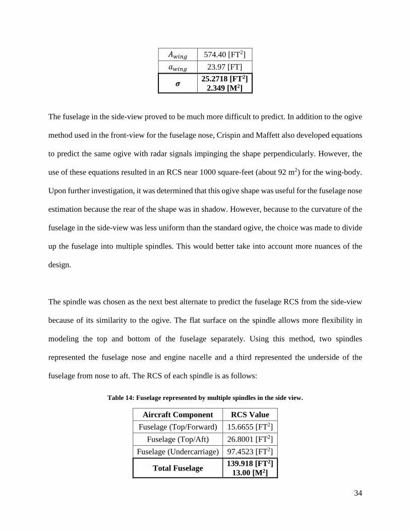
𝐴𝐴𝑤𝑤𝑖𝑖𝑤𝑤𝑤𝑤 574.40 [FT2] 𝜋𝜋𝑤𝑤𝑖𝑖𝑤𝑤𝑤𝑤 23.97 [FT]

𝝈𝝈 25.2718 [FT2] 2.349 [M2]

The fuselage in the side-view proved to be much more difficult to predict. In addition to the ogive

method used in the front-view for the fuselage nose, Crispin and Maffett also developed equations

to predict the same ogive with radar signals impinging the shape perpendicularly. However, the

use of these equations resulted in an RCS near 1000 square-feet (about 92 m2) for the wing-body.

Upon further investigation, it was determined that this ogive shape was useful for the fuselage nose

estimation because the rear of the shape was in shadow. However, because to the curvature of the

fuselage in the side-view was less uniform than the standard ogive, the choice was made to divide

up the fuselage into multiple spindles. This would better take into account more nuances of the

design.

The spindle was chosen as the next best alternate to predict the fuselage RCS from the side-view

because of its similarity to the ogive. The flat surface on the spindle allows more flexibility in

modeling the top and bottom of the fuselage separately. Using this method, two spindles

represented the fuselage nose and engine nacelle and a third represented the underside of the

fuselage from nose to aft. The RCS of each spindle is as follows:

Table 14: Fuselage represented by multiple spindles in the side view.

Aircraft Component RCS Value Fuselage (Top/Forward) 15.6655 [FT2]

Fuselage (Top/Aft) 26.8001 [FT2] Fuselage (Undercarriage) 97.4523 [FT2]

Total Fuselage 139.918 [FT2] 13.00 [M2]

35

It is clear from this analysis that the use of the spindle as an estimation of multiple portions of the

fuselage is much better than the ogive estimation of the entire aircraft fuselage. Unfortunately, the

spindle shape exposes just how high the fuselage contribution is in the side-view. The overall RCS

for the QF-36 in the side-view is as follows:

Table 15: Total RCS for the QF-36 in the side-view.

Component RCS Value Total Fuselage 139.918 [FT2]

Wing 25.2718 [FT2] Tail 0.2890 [FT2]

Total 165.4787 [FT2] 15.379[M2]

The penalty taken by the high RCS fuselage is seen immediately in the side-view estimation; the

side-view estimation RCS is nearly triple of the front-view.

36

5. Discussion and Design Implications

The development of this tool used to predict an aircraft’s RCS was proven successful by the trial

previously described. Not only were the results reasonable estimations, but they revealed patterns

that have been predicted in open source literature. According to some sources, there do exist

declassified RCS values for current and past aircraft. A list of these aircraft and their respective

RCS values is as follows and includes the comparison to the QF-36.

Table 16: Various RCS estimations for past and present military aircraft as well as the QF-36 concept.

Aircraft View RCS Value in M2 RCS Value in FT2 F-22A Raptor Generalized 0.00018 0.0019

F-35A Lightning II Generalized 0.00143 0.015 F-117A Nighthawk Generalized 0.001 to 0.01 0.01 to 0.1

B-1B Lancer Frontal 1 11 F-4 Phantom II Frontal 6 65 B-1A Excalibur Frontal 10 110

T-33 Shooting Star Frontal 10 110 T-33 Shooting Star Side 100 1100

B-70A Valkyrie Frontal 40 430 B-70A Valkyrie Side 105+ 106+

B-52 Stratofortress Frontal 100 1100 UCAV QF-36 Thunder Frontal 3.7 40 UCAV QF-36 Thunder Side 15.3 165

While this table serves as a decent resource of RCS values for several vehicles, it is important to

understand that because the wavelength used to calculate these RCS values is unknown, this is not

an ideal means of comparison. This tables serves as a basis for understanding where specific

aircraft lie, but there is the chance that each RCS was calculated using different radar systems

based on the technology relevant during their era of operation. For instance, the B-52 RCS could

have been calculated by radar systems relevant to the period in which the Stratofortress entered

37

service which was in 1955. On the other hand, the F-22 signature could be estimated using radar

relevant to today’s technological standards. While there is little that can be done to solve this

problem, the information still proves that the QF-36’s RCS predictions are on the correct scale.

The F-22 RCS was calculated based on a USAF news release claiming that the Raptor’s RCS was

that of a 15 millimeter diameter marble. Years later, the F-35 RCS was said to be that of “about a

golf ball” with a diameter of 4.3 centimeters [16]. What is important to keep in mind is that vehicles

including the F-22 and F-35 among others have other means of reducing their RCS values through

radar absorbing paint and onboard low-probability-of-intercept radar systems in addition to

purpose-shaping of the fuselage. It is unknown by how much radar absorbing paint and other

systems will further lower an aircraft’s RCS.

Table 15 shows how the QF-36 fits within the other jets and their known RCS estimations. The

wingspan of the QF-36 is 50 feet compared to the F-4’s 38 feet and F-117A’s 43 feet, and the QF-

36’s has an RCS that lies between that of the stealth jet and the fighter with respect to the front-

view. It is clear that the side-view of the QF-36 is rather high as it is near the T-33 side view RCS

value. However, the T-33 is only 38 feet compared to the QF-36’s 70 foot length.

With respect to the results, while the larger surfaces usually lend themselves to higher RCS values,

the tails proved to be the most unexpected feature. As seen in Table 11 and Table 14, the tails had

very small contributions to the overall RCS of the aircraft. Even on the broad side of the QF-36,

the protruding tails contributed little to the total RCS. Both the wing and the tail RCS values were

predicted using the flat plate equations, however, their impact on a specific view’s RCS was varied.

38

The wing made up 90-percent of the front-view RCS and 15-percent of the side-view. On the

contrary, the tail only made up 0.7-percent and 0.2-percent of the front- and side-view RCS values,

respectively. As well, even in the side-view, where a much larger surface area of the tail was

exposed, the tail RCS only changed by 0.5% from the front-view.

The following plot reveals the how the flat plate RCS estimation varies with increasing surface

area of the modeled component at a zero-degree incidence angle. In other words, the radar is

impinging the surface at its edge rather than its broad side.

Figure 17: Flat plate RCS estimation with tail and wing front-view examples.

As seen in the plot in Figure 17, the relationship between surface area and RCS is exponential.

Since the tail and wing differ drastically in size, this relationship between surface size and RCS is

important. The wing and tail surfaces are the two most crucial aspects of an aircraft. This is

especially true for the QF-36 since the UCAV has no need for a cockpit or any human factors-

related design features. These observations prove that changes to the tail and wing will impact the

overall RCS much differently. The results prove that even with large tail surfaces, the RCS

0 100 200 300 400 500 600 7000

5

10

15

20

25

30

35

40

Surface Area of Component (ft2)

RC

S V

alue

(ft2 )

Wing EstimationTail Estimation

39

contribution is always going to be much lower than the wing. It is therefore in a design engineer’s

best interest to minimize wing size and maximize tail size when meeting performance

specifications. With tails, larger horizontal stabilizers and rudders (or for this aircraft, a

“ruddervator”) provide for a more maneuverable the craft. Because the impact of the tail RCS is

so low, even drastic changes to the tail sizing will have a low impact on the RCS. Designers do

not have to compromise on performance objectives like spin recovery and tight turn radii. As well,

since the elevator can be rather large and no human is in the cockpit, the UCAV can meet its high

G load requirements at little cost to the RCS.

On the contrary, the exponential increase in RCS with surface area means that a large wing causes

a massive RCS contribution for each view. From a design perspective, this encourages the

minimization of the wing size which leads to smaller control surfaces and lessened roll

performance. Smaller wings also lessen the amount of fuel able to be carried internally onboard

the aircraft. With a high cruise and dash Mach number as well as a considerable range goal as set

by the AIAA RFP, the loss of volume for fuel could be crucial to meeting mission objectives.

In order to make up some of the losses in wing volume, a compromise can be made while

increasing the size of the fuselage. In the front-view, the fuselage only makes up 2.7-percent of

the total RCS for that view. For the side-view, the fuselage constitutes 85-percent. This drastic

difference suggests how the point of the fuselage shape diffuses the radar signal well, whereas the

side-view reflects much of the signal back to the receiver. The length of the aircraft can be changed

and with goals for a smaller wing, this is a plausible design option to consider. However, in order

to regain the fuel volume lost in the wings, it is possible to widen the fuselage at a low RCS penalty.

40

The previous plot shows that the change in fuselage width has a linear relationship to the RCS, but

even for an unreasonably large, ten-foot wide fuselage, the RCS increased by 67-percent to a mere

1.767 square-feet (0.1642 m2). This is still a meager five percent of the total front-view RCS. This

allows for the volume of the fuselage to be adjusted to accommodate any payload of fuel and radar

systems with little increase to the RCS. Unfortunately, the spindle used to estimate the side-view

of the fuselage does not taken into account the depth of the fuselage at that angle, only the height

and width. This would be an excellent start to a further investigation of the fuselage shape and its

impact on the RCS. Without a cockpit in the design, new fuselage shapes could be explored in

ways never before attempted.

Another possibility regarding the wing deals with the way in which it was modeled. The initial

attempt at calculating the RCS of the wing involved using total wing area seen forward looking

aft. This involved calculating the port and starboard wings as one, square flat plate. However,

looking aft, by modeling the wing as one instead of two surfaces, the estimation included a portion

of the wing that lies in shadow of the fuselage nose. As a further investigation, the wing was then

modeled as two separate flat plate surfaces in an attempt to compare it to the single plate model.

0 1 2 3 4 5 6 7 8 9 10 11 120

0.5

1

1.5

2

2.5

Fuselage Width (ft)

RC

S V

alue

(ft2 )

Fuselage 6ft wideFuselage 10ft wide

41

The resulting RCS of each wing was 9.0828 square-feet (0.8441 m2) making the total wing RCS

18.1656 square-feet (1.6883 m2). This is a reduction in wing RCS of nearly 50-percent. This shows

how by modeling each component with more and more detail, a more thorough and accurate RCS

of the total aircraft can be calculated. While less shapes and less detail capture the initial RCS, the

more effort that goes into modeling each component will surely produce a more accurate RCS.

This may result in the fluctuation of each view’s RCS.

42

6. Conclusion

This research demonstrates the feasibility of predicting an aircraft’s radar echo, or RCS, using

open-source equations for simple shapes. Because of the classified and time-consuming nature of

calculating exact RCS values, this tool could be used throughout the aircraft design process as a

means of understanding which components of the vehicle contribute the most to the overall RCS.

Not only does this tool save time and effort, but it also provides the designer with more information

earlier in the design process. Stealth is one of the newest frontiers relevant to aircraft design and

will continue to be so long as radar remains relevant. With this in mind, any tools created to help

integrate new design techniques relevant to stealth are important as they streamline the efforts of

designers and alleviate their workload. It is for these reasons among others that this research has

relevance to the current field of military aircraft design.

With respect to the QF-36, the methodology developed for calculating RCS gave insight into which

areas of the aircraft to concentrate efforts in order to reduce the overall RCS. While its RCS was a

reasonable value compared to other craft, the UCAV’s unique and pilotless mission allow for

adjustments to further reduce the RCS. To accommodate more fuel and stores, a high fuselage

volume can be made with little increase in the overall signature size. As well, it is clear that a

compromise will need to be made with regards to the control surface sizing. The wing has a high

contribution of RCS in both the front- and side-views. In contrast, however, the tails contributed

much less than expected in both analyses of RCS. This allows for maximized turn and spin

recovery performance with next to no impact on the RCS. These observations are crucial to

realizing the power of this tool. In future iterations of the QF-36, more and more detailed analyses

43

of components can be completed leading to a more refined and intelligently designed aircraft

concept.

44

References

[1] Skolnik, Merrill I., “Radar (electronics),” Encyclopedia Britannica Online, 2 Aug 2013.

Web. 09 Sept 2014, http://www.britannica.com/EBchecked/topic/488278/radar.

[2] "Stealth Technology and the Counter-stealth Response." Air Force Technology. Kable

Intelligence Limited, 25 Aug. 2011. Web. 08 Sept. 2014, http://www.airforce-

technology.com/features/feature128011/.

[3] Cadirci, Serdar, “RF Stealth (or Low Observable) and Counter-RF Stealth Technologies:

Implications of Counter-RF Stealth Solutions for Turkish Air Force,” Naval Postgraduate

School, 2009.

[4] Crispin, J. W., Maffett, A. L., “Radar Cross-Section Estimation for Simple Shapes,”

Proceedings of the IEEE, 1965.

[5] Dimitris V. Dranidis, “Airborne Stealth in a Nutshell-Part I,” the Magazine of the

Computer Harpoon Community http://www.harpoonhq.com/waypoint/. (Accessed

February 2015).

[6] Roskam, Jan. Airplane Design. Vol. Part 1: Preliminary Sizing of Airplanes. Ottawa:

Roskam Aviation and Engineering Corporation, 1985. Print.

[7] United States. Government Accountability Office. Defense Acquisitions Assessment of

Selected Weapons Programs. By Michael J. Sullivan. 2011. Print. GAO-11-233SP.

[8] “The Electromagnetic Spectrum: Radio Waves.” NASA Science Headquarters. Web. 12

Dec 2015, http://science.hq.nasa.gov/kids/imagers/ems/radio.html.

[9] “Low-frequency radar,” Wikipedia, 26 Jan 2016. Web. 28 Jan 2016,

https://en.wikipedia.org/wiki/Low-frequency_radar.

45

[10] O’Donnell, Robert M., “Radar Systems Engineering, Lecture 7 – Part 1, Radar Cross

Section”, IEEE New Hampshire Section, 2010.

[11] Wolff, Christian, “Waves and Frequency Ranges”, Radar Basics. Web. 1 Feb 2016,

http://www.radartutorial.eu/07.waves/Waves%20and%20Frequency%20Ranges.en.html.

[12] Wolff, Christian, “MEADS”, Card Index of Radar Sets - Battlefield. Web. 1 Feb 2016,

http://www.radartutorial.eu/19.kartei/karte410.en.html.

[13] Anthropometry and biomechanics, Web. 15 Feb 2016. http://www.ergo-

eg.com/uploads/digi_lib/116.pdf

[14] “Anthropometry and Biomechanics Related Design Data”, NASA Man-Systems Integration

Standards. Web. 15 Feb 2016. http://msis.jsc.nasa.gov/sections/section03.htm

[15] Hott, Bartholomew, Pollock, George E. “The Adevent, Evolution, and New Horizons of

United States Stealth Aircraft.” Web. 18 Feb 2016.

http://web.ics.purdue.edu/~gpollock/The%20Advent,%20Evolution,%20and%20New%20

Horizons%20of%20United%20States%20Stealth%20Aircraft.htm

[16] “RCS of Typical Radar Targets”. Web. 31 March 2016.

http://www.alternatewars.com/BBOW/Radar/Radar_Targets.htm

Appendix A: AIAA Request for Proposal

A2

A3

A4

A5

A6

A7

A8

A9

Appendix B: QF-36 Concept Design Drawings

B2

Figure B 1: Three-view drawing of UCAV QF-36 with dimensions.

Figure B2: UCAV QF-36, view 1.

B3

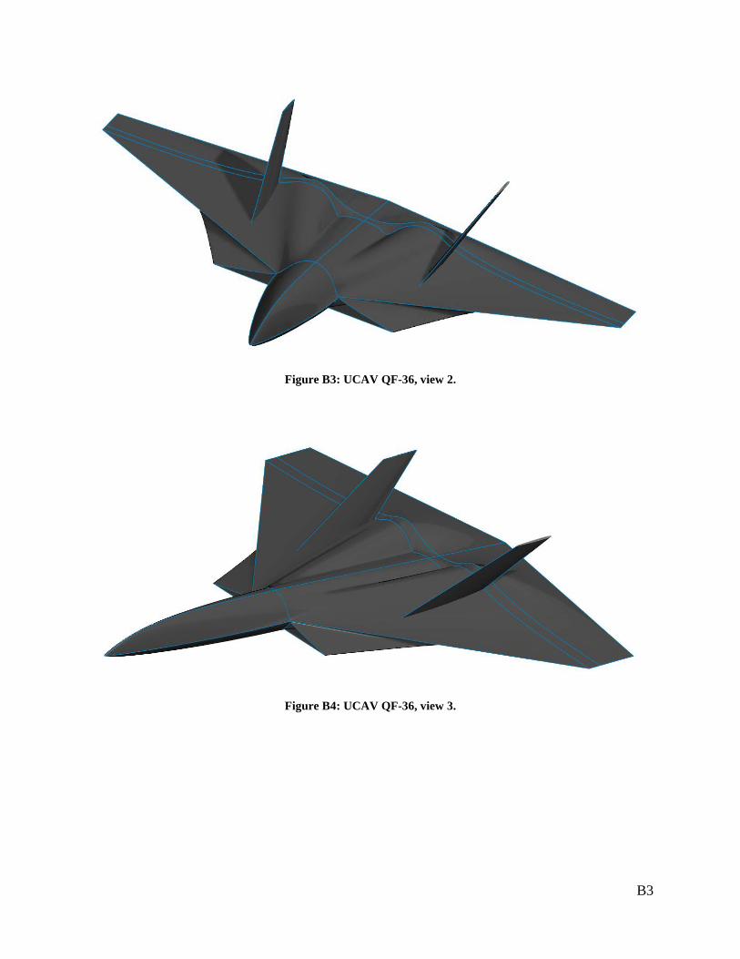
Figure B3: UCAV QF-36, view 2.

Figure B4: UCAV QF-36, view 3.

B4

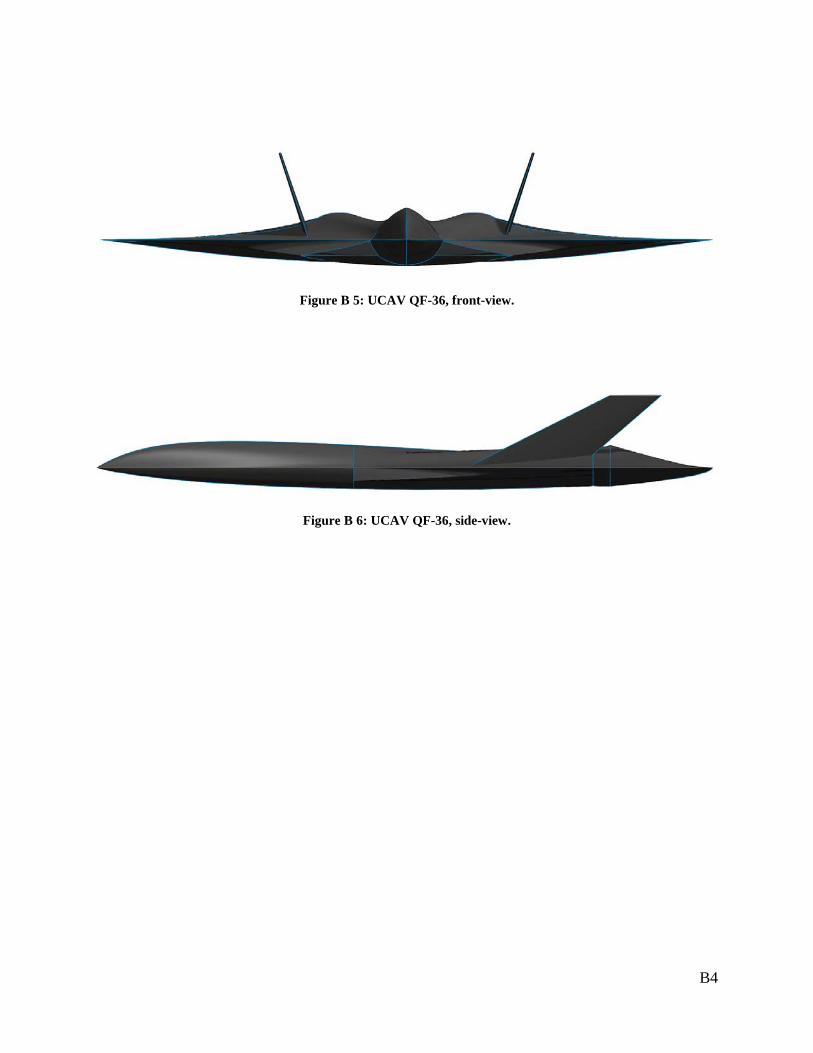
Figure B 5: UCAV QF-36, front-view.

Figure B 6: UCAV QF-36, side-view.

B5

Figure B 7: UCAV QF-36, top view.