approaches to clustering gene expression time course data · approaches to clustering gene...
TRANSCRIPT
Approaches to clustering gene expression time
course data
by
Praveen Krishnamurthy
August, 2006
A thesis submitted to
The Faculty of the Graduate School of
The State University of New York at Buffalo
in partial fulfillment of the requirements for the degree of
Master of Science
Department of Computer Science and Engineering
Abstract
Conventional techniques to cluster gene expression time course data have either ignored the
time aspect, by treating time points as independent, or have used parametric models where the
model complexity has to be fixed beforehand. In this thesis, we have applied a non-parametric
version of the traditional hidden Markov model (HMM), called the hierarchical Dirichlet process -
hidden Markov model (HDP-HMM), to the task of clustering gene expression time course data. The
HDP-HMM is an instantiation of an HMM in the hierarchical Dirichlet process (HDP) framework
of Teh et al. (2004), in which we place a non-parametric prior on the number of hidden states of
an HMM that allows for a countably infinite number of hidden states, and hence overcomes the
issue of fixing model complexity. At the same time, by having a Dirichlet process in a hierarchical
framework we let the same countably infinite set of “next states” in the Markov chain of the HMM
be shared without constraining the flexible architecture of the model. We describe the algorithm
in detail and compare the results obtained by our method with those obtained from traditional
methods on two popular datasets - Iyer et al. (1999) and Cho et al. (1998). We show that a non-
parametric hierarchical model such as ours can solve complex clustering tasks effectively without
having to fix the model complexity beforehand and at the same time avoids overfitting.

Acknowledgements
I would like to thank my advisor, Matthew J. Beal, for his support and guidance. Two years
ago when I started my Masters program, I had no idea it would turn out this way. I’ve learnt a lot
in the area of Machine Learning and it has been a wonderful experience working with him.
I would also like to thank Dr. Aidong Zhang for her inputs in the Bioinformatics course. That
was my first introduction to bioinformatics, and has helped a lot me in this thesis.
I would like to acknowledge my colleagues - Rahul Krishna, whose notes came in handy in the
description of Dirichlet Processes and Hierarchical Dirichlet Processes. And Shravya Shetty for
proof reading this manuscript.

Contents
1 Introduction 5
1.1 Gene expression . . . . . . . . . . . . . . . . . . . . . . . . . . . . . . . . . . . . . . . 5
1.1.1 Microarrays . . . . . . . . . . . . . . . . . . . . . . . . . . . . . . . . . . . . . 6
1.1.2 Time series data . . . . . . . . . . . . . . . . . . . . . . . . . . . . . . . . . . 8
1.2 Clustering genes . . . . . . . . . . . . . . . . . . . . . . . . . . . . . . . . . . . . . . 9
1.2.1 The task . . . . . . . . . . . . . . . . . . . . . . . . . . . . . . . . . . . . . . . 9
1.2.2 Challenges . . . . . . . . . . . . . . . . . . . . . . . . . . . . . . . . . . . . . 10
2 Literature Review 11
2.1 Clustering . . . . . . . . . . . . . . . . . . . . . . . . . . . . . . . . . . . . . . . . . . 11
2.1.1 Clustering methodologies . . . . . . . . . . . . . . . . . . . . . . . . . . . . . 11
2.1.2 Cluster validation . . . . . . . . . . . . . . . . . . . . . . . . . . . . . . . . . 12
2.1.3 Approaches to clustering gene expression time-course data . . . . . . . . . . . 17
2.1.4 Tree based metrics . . . . . . . . . . . . . . . . . . . . . . . . . . . . . . . . . 19
3 Methods for clustering genes 21
3.1 Correlation analysis . . . . . . . . . . . . . . . . . . . . . . . . . . . . . . . . . . . . 21
3.2 Statistical approaches to cluster time series data . . . . . . . . . . . . . . . . . . . . 22
3.2.1 CAGED - Cluster analysis of gene expression dynamics . . . . . . . . . . . . 22
3.2.2 Finite HMM with Gaussian output . . . . . . . . . . . . . . . . . . . . . . . . 25
3.2.3 Other approaches . . . . . . . . . . . . . . . . . . . . . . . . . . . . . . . . . . 27
3

CONTENTS 4
4 The infinite hidden Markov model 29
4.1 Notation . . . . . . . . . . . . . . . . . . . . . . . . . . . . . . . . . . . . . . . . . . . 30
4.2 Dirichlet Processes . . . . . . . . . . . . . . . . . . . . . . . . . . . . . . . . . . . . . 31
4.2.1 The Polya urn scheme and the Chinese restaurant process . . . . . . . . . . . 31
4.2.2 The stick-breaking construction . . . . . . . . . . . . . . . . . . . . . . . . . . 34
4.2.3 Dirichlet process mixture model . . . . . . . . . . . . . . . . . . . . . . . . . 35
4.3 Hierarchical Dirichlet processes . . . . . . . . . . . . . . . . . . . . . . . . . . . . . . 36
4.3.1 The stick-breaking construction . . . . . . . . . . . . . . . . . . . . . . . . . . 37
4.3.2 The Chinese restaurant franchise . . . . . . . . . . . . . . . . . . . . . . . . . 38
4.4 The infinite hidden Markov model . . . . . . . . . . . . . . . . . . . . . . . . . . . . 40
4.4.1 Hidden Markov models . . . . . . . . . . . . . . . . . . . . . . . . . . . . . . 40
4.4.2 HDP-HMM . . . . . . . . . . . . . . . . . . . . . . . . . . . . . . . . . . . . . 41
4.4.3 Applications . . . . . . . . . . . . . . . . . . . . . . . . . . . . . . . . . . . . 43
5 Experiments 45
5.1 Datasets . . . . . . . . . . . . . . . . . . . . . . . . . . . . . . . . . . . . . . . . . . . 45
5.2 Design . . . . . . . . . . . . . . . . . . . . . . . . . . . . . . . . . . . . . . . . . . . . 46
5.3 Results . . . . . . . . . . . . . . . . . . . . . . . . . . . . . . . . . . . . . . . . . . . . 48
5.4 Interpretation . . . . . . . . . . . . . . . . . . . . . . . . . . . . . . . . . . . . . . . . 50
6 Conclusion 56
6.1 Future directions . . . . . . . . . . . . . . . . . . . . . . . . . . . . . . . . . . . . . . 57
Appendices 62
A Dirichlet Process theory 62
Chapter 1
Introduction
Genes are the units of heredity in living organisms. They are encoded in the organism’s genetic
material, and control the physical development and behavior of the organism. During reproduction,
the genetic material is passed on from the parent(s) to the offspring. Genes encode the information
necessary to construct the chemicals (proteins etc.) needed for the organism to function.
Following the discovery that Deoxyribonucleic acid (DNA) is the genetic material, the common
usage of the word ‘gene’ has increasingly reflected its meaning in molecular biology, namely the
segments of DNA which cells transcribe into Ribonucleic acid (RNA) and translate into proteins.
The Sequence Ontology project defines a gene as: “A locatable region of genomic sequence, corre-
sponding to a unit of inheritance, which is associated with regulatory regions, transcribed regions
and/or other functional sequence regions”.
1.1 Gene expression
Gene expression, often simply called expression, is the process by which a gene’s DNA sequence is
converted into the structures and functions of a cell.
Gene expression is a multi-step process that begins with transcription of DNA, which genes
are made of, into messenger RNA. It is then followed by post-transcriptional modification and
translation into a gene product, followed by folding, post-translational modification and targeting.
The amount of protein that a cell expresses depends on the tissue, the developmental stage of
5

CHAPTER 1. INTRODUCTION 6
the organism and the metabolic or physiologic state of the cell.
1.1.1 Microarrays
Microarray refers to both the process and the technology used to measure the expression of par-
ticular genes. Microarray technology or more specifically DNA microarray technology provides a
rough measure of the cellular concentration of different messenger RNAs (mRNA).
A DNA microarray (also known as a gene chip, or bio chip, or DNA chip) is a collection of
microscopic DNA spots attached to a solid surface, such as glass, plastic or silicon chip forming an
array for the purpose of monitoring of expression levels.
The affixed DNA segments are known as probes, thousands of which can be used in a single DNA
microarray. Measuring gene expression using microarrays is relevant to many areas of biology and
medicine, such as studying treatments, disease, and developmental stages. For example, microarrays
can be used to identify disease genes by comparing gene expression in disease and normal cells.
DNA microarrays can be used to detect RNAs that may or may not be translated into active
proteins. Scientists refer to this kind of analysis as “expression analysis” or expression profiling.
Since there can be tens of thousands of distinct reporters on an array, each microarray experiment
can accomplish the equivalent of a number of genetic tests in parallel. Arrays have therefore
dramatically accelerated many types of investigations.
Depending upon the kind of immobilized sample used construct arrays and the information fetched,
the microarray experiments can be categorized in three ways:
1. Microarray expression analysis: In this experimental setup, the complimentary DNA (cDNA)
derived from the mRNA of known genes is immobilized. The sample has genes from both the
normal as well as the diseased tissues. Spots with more intensity are obtained for diseased
tissue gene if the gene is over expressed in the diseased condition. This expression pattern is
then compared to the expression pattern of a gene responsible for a disease.
2. Microarray for mutation analysis: For this analysis, the researchers use genomic DNA (gDNA).
The genes might differ from each other by as less as a single nucleotide base. A single base
difference between two sequences is known as Single Nucleotide Polymorphism (SNP).

CHAPTER 1. INTRODUCTION 7
Figure 1.1: A typical dual-color microarray used in expression analysis
3. Comparative Genomic Hybridization: is used for the identification in the increase or decrease
of the important chromosomal fragments harboring genes involved in a disease.
A few applications of microarrays are:
1. Gene discovery: Microarray experiments helps in the identification of new genes, know about
their functioning and expression levels under different conditions.
2. Disease diagnosis: Microarray technology helps researchers learn more about different diseases
such as heart diseases, mental illness, infectious disease and especially the study of cancer.
Until recently, different types of cancer have been classified on the basis of the organs in which
the tumors develop. Now, with the evolution of microarray technology, it will be possible for
the researchers to further classify the types of cancer on the basis of the patterns of gene
activity in the tumor cells. This will tremendously help the pharmaceutical community to
develop more effective drugs as the treatment strategies will be targeted directly to the specific
type of cancer.
3. Drug discovery: Microarray has extensive application in Pharmacogenomics. Pharmacoge-
nomics is the study of correlations between therapeutic responses to drugs and the genetic
profiles of the patients. Comparative analysis of the genes from a diseased and a normal cell

CHAPTER 1. INTRODUCTION 8
will help the identification of the biochemical constitution of the proteins synthesized by the
diseased genes. The researchers can use this information to synthesize drugs which combat
with these proteins and reduce their effect.
4. Toxicological research: Toxicogenomics establishes correlation between responses to toxicants
and the changes in the genetic profiles of the cells exposed to such toxicants.
1.1.2 Time series data
Time series data for gene expression is obtained when expression values are read off at various
time points during a single experiment. Oftentimes many experiments are run in parallel and
stopped for measurement one by one at allotted time points; this is particularly true for mammalian
experiments where DNA measurement requires the sacrifice of the subject. While this procedure
does not produce a pure single time course, and instead one made from many terminating time
courses, biologists and bioinformaticians do consider it viable time course data.. Expression values
can be read off at equal or unequal intervals of time. The primary goal of collecting time series data
is to gain insight into understanding genetic regulatory networks (GRN). A GRN is a collection
of DNA segments in a cell which interact with each other and with other substances in the cell,
thereby governing the rates at which genes in the network are transcribed into mRNA.
Regulation of gene expression (gene regulation) is the cellular control of the amount and timing
of appearance (induction) of the functional product of a gene. Although a functional gene product
may be an RNA or a protein, the majority of the known mechanisms regulate the expression
of protein coding genes. Any step of gene expression may be modulated, from the DNA-RNA
transcription step to post-translational modification of a protein. Gene regulation gives the cell
control over structure and function, and is the basis for cellular differentiation, morphogenesis and
the versatility and adaptability of any organism.
Two genes are said to co-express when they have similar expression patterns, and they are
said to co-regulate when they are regulated by common transcription factors. Viewed from the
co-expression point of view, co-regulation would lead to similar expression patterns over time as
the genes are regulated by common transcription factors. Hence, similar expression pattern over
CHAPTER 1. INTRODUCTION 9
time could give important information regarding the underlying genetic regulatory networks.
1.2 Clustering genes
There are about 25,000 genes in a human being, and only a few of them have been completely
analyzed, annotated and well understood. Understanding genes and their functionality remains a
prime objective of human genome researchers.
Why do we need to understand genes?
1. Disease diagnosis: Understanding genes can help in understanding the causes of diseases at
the cellular level. For example, cancer classification can be done based on patterns of gene
activity in the tumor cells.
2. Gene discovery: Understanding genes can aid in understanding the functionality of unknown
genes. As mentioned earlier, very few genes have been completely understood, so discovery of
new genes is an important step in understanding and building a comprehensive gene database.
3. Gene therapy: is the insertion of genes into an individual’s cells and tissues to treat a dis-
ease, and hereditary diseases in particular. Gene therapy is still in its infancy, and a better
understanding of genes would help devising effective therapies.
4. Gene expression analysis of one gene at a time has provided a wealth of biological insight,
however analysis at a genome level is yet to be carried out.
1.2.1 The task
Given that we have gene expression time-course data, our task is to cluster them into groups of
genes with similar expression patterns over time. Such a task can be unsupervised - in which case
we have no information regarding any of the genes being analyzed, or it can be supervised - wherein
genes are clustered based on their similarity to known genes. We undertake the former task, as it
is can be applied even in the absence of labeled data, and in many a case is an important step in
the latter task.

CHAPTER 1. INTRODUCTION 10
1.2.2 Challenges
Clustering gene expression time-course data is not a trivial task. Not only does it involve devising
a measure of similarity for genes, but also involves the tricky problem of identifying the number of
true clusters. Some of the problems that need to be taken care of in devising a method to cluster
time series data are:
1. Due to the high throughput of microarrays, the levels of error and noise in the measurements
are high.
2. Data is often incomplete with many missing values.
3. Unequal time interval between successive time points.
4. Genes can be involved in several pathways and have multiple functions depending on specifics
of the cell’s environment. Hence, groups of genes defined according to similarity of function
or regulation of a gene are not disjoint in general.
In this chapter we have described some of the concepts involved in gene expression analysis like
gene expression, microarrays, gene regulation, time-course data etc.. We have also defined the task
of clustering gene expression time-course data. The rest of the thesis reviews some of the methods
researchers have adopted to solve this task, and our approach towards the problem.

Chapter 2
Literature Review
2.1 Clustering
Clustering is the partitioning of a data set into (disjoint) subsets, called clusters, so that the data
in each subset share some common trait - often proximity according to some well-defined distance
measure. Clustering is mostly seen as an unsupervised problem - where in no labeled data is
available. Based on the technique used to create clusters and the proximity measure, one can have
many clustering methods.
2.1.1 Clustering methodologies
Clustering methods broadly fall into one of the following categories:
1. Partition based clustering: In a partition based clustering algorithm, data is divided into
mutually exclusive groups so as to optimize a certain cost function. An example of cost
function could be sum of distances of all points from their respective cluster centroids. Such a
cost function aims to produce clusters which are tight and compact, and this clustering method
is called the k-means clustering. Partition based clustering generally involve reassignment of
data points to clusters in successive iterations to obtain a locally optimal value for the cost
function.
2. Hierarchical clustering: algorithms find successive clusters using previously established clus-
11
CHAPTER 2. LITERATURE REVIEW 12
ters (unlike partition based algorithms which determine all clusters at once). Hierarchical
algorithms can be agglomerative (bottom-up) or divisive (top-down). Agglomerative algo-
rithms begin with each element as a separate cluster and merge them in successively larger
clusters. Divisive algorithms begin with the whole set and proceed to divide it into succes-
sively smaller clusters.
3. Density based clustering: involves the density-based notion (not to be confused with proba-
bility density) of a cluster. A cluster is defined as a maximal set of density-connected points.
Density Based Clustering starts by estimating the density for each point in order to identify
core, border and noise points. A core point is referred to as a point whose density is greater
than a user-defined threshold. Similarly, a noise point is referred to as a point whose density
is less than a user-defined threshold. Noise points are usually discarded in the clustering
process. A non-core, non-noise point is considered as a border point. Hence, clusters can be
defined as dense regions (i.e. a set of core points), and each dense region is separated from
one another by low density regions (i.e. a set of border points).
An increasingly popular approach to similarity based clustering (and segmentation) is by spectral
methods. These methods use eigenvalues and eigenvectors of a matrix constructed from the pairwise
similarity function. Given a set of data points, the similarity matrix may be defined as a matrix
S, where Sij represents a measure of the similarity between point i and j. Spectral clustering
techniques make use of the spectrum of the similarity matrix of the data to cluster the points.
2.1.2 Cluster validation
One of the most important issues in cluster analysis is the evaluation of clustering results to find
the partitioning that best fits the underlying data. By validating clusters obtained by a clustering
algorithm, we assess the quality and reliability of clustering result. Some of the reasons why we
require validation are:
1. To check if clustering is formed by chance. Clustering by chance is more severe when the
number of clusters/classes is small.
2. To compare different clustering algorithms.

CHAPTER 2. LITERATURE REVIEW 13
3. To choose clustering parameters. Typically, in an unsupervised learning environment, the
number of classes/labels is not known beforehand, hence this parameter is provided as an
input to the clustering algorithm. Validation can help fixing this parameter. Some of the
other parameters that clustering algorithms require are density and radius (in density based
clustering algorithms).
4. When the data is high dimensional, effective visualization of clustering result is often difficult
and may not be the best method to evaluate the quality of the clustering. Hence, a more
objective approach to validate clusters is preferable.
Cluster validation is usually done by computation of indices. Indices are scores which signify
the quality of clustering. There are 2 kinds of indices - external and internal. External indices are
obtained by comparison of clustering result with the ground truth or some pre-defined partition of
the data which reflects our intuition about the clusters, whereas internal indices do not depend on
any external reference and use only the data to validate clusters.
External indices
As mentioned before, external indices are computed by comparison with ground truth. Let N be the
number of data points. Let P ′ = {P1, ..., Pm} be the ground truth clusters. Let C ′ = {C1, ..., Cn}
be the clustering obtained by a clustering algorithm. We define two N x N ‘incidence’ matrices (P
and C), where the rows and columns both correspond to data points, as follows - Pij = 1, if both
the ith point and the jth point belong to same cluster in P ′; 0 otherwise. And, Cij = 1, if both the
ith point and the jth point belong to same cluster in C ′; 0 otherwise. A pair of data points, i and
j, can fall into one of the following categories (S meaning Same and D meaning Different):
SS : Cij = 1 and Pij = 1
DD : Cij = 0 and Pij = 0
SD : Cij = 1 and Pij = 0
DS : Cij = 0 and Pij = 1

CHAPTER 2. LITERATURE REVIEW 14
1. Rand index - With the above notation, the Rand index is defined as:
Rand =|SS|+ |DD|
|SS|+ |SD|+ |DS|+ |DD|(2.1)
2. Jaccard coefficient - A potential problem with Rand index is that the figure |DD| can be very
high, hence skewing the result. In order to get around this problem, the Jaccard coefficient
is defined as:
Jaccard =|SS|
|SS|+ |SD|+ |DS|(2.2)
3. Corrected Rand index - Milligan (1986) has corrected the Rand index for chance, and the
resulting index is called the Corrected Rand index. Corrected Rand (CR) is defined as:
CR =
∑mi=1
∑nj=1
(nij
2
)−(n2
)−1∑mi=1
(ni∗2
)∑nj=1
(n∗j
2
)12
[∑mi=1
(ni∗2
)+∑n
j=1
(n∗j
2
)]−(n2
)−1∑mi=1
(ni∗2
)∑nj=1
(n∗j
2
) (2.3)
where nij represents the number of points in cluster Pi and Cj , ni∗ indicates the number
of points in cluster Pi, n∗j indicates the number of points in cluster Cj , and n is the total
number of points.
Internal indices
Ground truth may not always be available. In such cases, internal indices are computed to quan-
titatively assess clustering. Internal indices try to evaluate two aspects that any good clustering
algorithm should possess: cohesion - how similar or how close are points belonging to the same
cluster, and separation - how dissimilar or how far are points belonging to different clusters. Most
common internal indices use Sum of Squared Error (or SSE) computation. Cohesiveness of a clus-
ter is measured by sum of squares of intracluster distances between the points in a cluster. This
quantity, called WSS, is given by:
WSS =∑i
∑x∈Ci
(x−mi)2 (2.4)

CHAPTER 2. LITERATURE REVIEW 15
where, i is the index over the number of clusters, x is a data point, Ci is the ith cluster, and mi is
the centroid of the ith cluster.
Separation is measured by sum of squares of inter-cluster distances. This quantity, called BSS, is
the given by:
BSS =∑i
|Ci| (m−mi)2 (2.5)
where, i is the index over the number of clusters, |Ci| is the number of points assigned to the ith
cluster, m is the centroid of the whole data set, and mi is the centroid of the ith cluster. It is clear
that a good clustering algorithm would aim to increase BSS and reduce WSS. A property of these
indices is that their sum (i.e. WSS+BSS) is a constant and larger number of tight clusters result
in smaller WSS. In fact, the ratio BSS/WSS is used an indicator of the quality of clustering.
As seen, external indices are measured with respect to the ground truth, which is ideal in terms
of a quantitative measurement of clustering performance, but not always is a labeling of the data
available and one needs to resort to internal indices. Internal indices give a quantitative assessment
of what are actually qualitative heuristics, such as compactness or exclusivity of clusters, and do
not depend on an external labeling. Such indices are likely to be subject to interpretation, and the
significance of these indices to our experiments will be discussed in later chapters.
Relative Indices
Apart from the above kinds of indices, there is a third kind of index - the relative index. Relative
indices are used primarily to compare various clustering algorithms or results. Relative indices can
be used to find good values for input parameters of certain algorithms. Given below are three such
relative indices.
1. Silhouette index: For a given cluster, Cj (j = 1, ...,m), this method assigns to each sample of
Cj a quality measure, s(i) (i = 1, ..., n), known as the Silhouette width. The Silhouette width
is a confidence indicator on the membership of the ith sample in cluster Cj . The Silhouette
width for the ith sample in cluster Cj is defined as:
s(i) =b(i)− a(i)
max{a(i), b(i)}(2.6)
CHAPTER 2. LITERATURE REVIEW 16
where a(i) is the average distance between the ith sample and all of the samples included in
Cj , and b(i) is the minimum average distance between the ith sample and all of the samples
clustered in Ck (k = 1, ...,m; k 6= j). From this formula it follows that −1 ≤ s(i) ≤ 1.
When a s(i) is close to 1, one may infer that the ith sample has been well clustered, i.e. it
was assigned to an appropriate cluster. When a s(i) is close to zero, it suggests that the ith
sample could also be assigned to the nearest neighboring cluster. If s(i) is close to -1, one may
argue that such a sample has been misclassified. Thus, for a given cluster, Cj (j = 1, ...,m),
it is possible to calculate a cluster Silhouette Sj , which characterizes the heterogeneity and
isolation properties of such a cluster:
Sj =1n
n∑i=1
s(i) (2.7)
where n is number of samples in Cj . It has been shown that for any partition U ↔ C :
C1, C2, ...Cm, a Global Silhouette value, GSu, can be used as an effective validity index.
GSu =1m
m∑j=1
Sj (2.8)
Furthermore, it has been demonstrated that equation can be applied to estimate the most
appropriate number of clusters for the data set. In this case the partition with the maximum
GSu is taken as the optimal partition.
2. Dunn’s Index: This index identifies sets of clusters that are compact and well separated. For
any partition, U, produced by a clustering algorithm, let Ci represent the ith cluster, the
Dunn’s validation index, D, is defined as:
D(U) = min1≤i≤m
min1≤i≤mj 6=i
{δ(Ci, Cj)
max1≤k≤m {∆(Ck)}
} (2.9)
where δ(Ci, Cj) defines the distance between clusters Ci and Cj (intercluster distance); ∆(Ck)
represents the intracluster distance of cluster Ck, and m is the number of clusters of parti-
tion. The main goal of this measure is to maximize intercluster distances whilst minimizing

CHAPTER 2. LITERATURE REVIEW 17
intracluster distances. Thus large values of D correspond to good clusters. Therefore, the
number of clusters that maximizes D is taken as the optimal number of clusters, m.
3. Davies-Bouldin Index: Like the Dunns index, the Davies-Bouldin index aims at identifying
sets of clusters that are compact and well separated. The Davies-Bouldin validation index,
DB, is defined as:
DB(U) =1m
m∑i=1
maxj 6=i
{∆(Ci) + ∆(Cj)
δ(Ci, Cj)
}(2.10)
where U , δ(Ci, Cj), ∆(Ci), ∆(Cj) and m are defined as in equation (2.9). Small values of
DB correspond to clusters that are compact, and whose centers are far away from each other.
Therefore, the cluster configuration that minimizes DB is taken as the optimal number of
clusters, m.
2.1.3 Approaches to clustering gene expression time-course data
Given the various clustering algorithms and validation techniques, there are a multitude of com-
binations one can use to cluster a data set and validate the cluster. Clustering algorithms and
validation techniques use basic distance, intercluster and intracluster distance metrics in the eval-
uation of cost function. Below, we give commonly used distance metrics. The following notation
has been used in the description of the metrics: x and y denote points in n-dimensional space, and
the components of the points be x1, x2, . . . , xn. Let S and T denote two clusters.
Basic distance metrics
The distance between two data points (genes) can be one of the following:
1. Euclidean distance: For any two points, the Euclidean distance between then is geometric dis-
tance between them in the n-dimensional space. Euclidean distance is the 2-norm (sometimes
called the Euclidean norm), and is given by
d =
(n∑i=1
(xi − yi)2) 1
2
CHAPTER 2. LITERATURE REVIEW 18
2. Manhattan distance: between two points in an Euclidean space is the sum of the lengths of
the projections of the line segment between the points onto the coordinate axes. Manhattan
distance is also called the 1-norm or taxicab distance, and is given by
d =n∑i=1
(xi − yi)
3. Correlation similarity: The correlation between two n-dimensional points can be used a sim-
ilarity measure between the two genes. As an example, the Pearson correlation coefficient
between two n-dimensional points is given by
d =∑n
i=1(xi − µx)(yi − µy)(n− 1)σxσy
where µx is the mean of x, and σx is its standard deviation.
4. Cosine similarity: If the data points can be considered as vectors in an n-dimensional space,
then the ratio of the dot product of the vectors to the product of their magnitudes gives
the cosine of the angle between the vectors. This value can be used as a similarity measure
between the vectors. The cosine distance between two points is given by
d =∑n
i=1 xiyi√(∑ni=1 x
2i
) (∑ni=1 y
2i
)5. Probabilistic: A probabilistic model can be used to evaluate the distance between two data
points. The probabilistic score obtained by such a model can be used as a similarity measure
between the two points.
The last three measures are similarity measures, hence their inverse is used as a distance measure.
These measures are, strictly speaking, not distance measures as they may not satisfy the triangle
inequality property, however they still find heavy usage in clustering.

CHAPTER 2. LITERATURE REVIEW 19
Intercluster distance metrics
1. The single linkage distance defines the closest distance between two points belonging to two
different clusters.
2. The complete linkage distance represents the distance between the most remote points be-
longing to two different clusters.
3. The average linkage distance defines the average distance between all of the points belonging
to two different clusters.
4. The centroid linkage distance reflects the distance between the centers of two clusters.
5. The average of centroids linkage represents the distance between the center of a cluster and
all of samples belonging to a different cluster.
Intracluster distance metrics
1. The complete diameter distance represents the distance between the most remote points
belonging to the same cluster.
2. The average diameter distance defines the average distance between all the points belonging
to the same cluster.
3. The centroid diameter distance reflects the double average distance between all of the points
and the centroid of the cluster.
2.1.4 Tree based metrics
Hierarchical clustering algorithms give rise to a tree structure, in which the data points can be
viewed as leaves and clusters are ‘built’ by merging points close to each other and this process
continuing with the resulting clusters. The resultant tree-like structure is called a ‘dendrogram’
and has a property that the level at which two points are merged is indicative of the proximity of
the points. The process of merging continues all the way to the point we have one cluster. And a
partition of the data can be obtained by ‘severing’ the dendrogram at a required level. Despite the

CHAPTER 2. LITERATURE REVIEW 20
wide use of hierarchical clustering algorithms, there is very little literature on assessing the quality
of dendrograms resulting from such algorithms. Wild et al. (2002) have devised three (related)
quantitative measures which assess the quality of dendrogram, namely - Dendrogram purity, Leaf
Harmony, and Leaf Disparity. Let T be a dendrogram tree structure and C be a set of class labels
for the leaves of the tree.
1. Dendrogram Purity(T , C): Let L = {1, 2, . . . , L} be the set of leaves and C = {c1, c2, . . . , cL}
be the class assignment for each leaf. Dendrogram purity is defined to be the measure obtained
from the following random process: pick a leaf l at random. Pick another leaf j in the same
class as l. Find the smallest subtree containing l and j. Measure the fraction of leaves in
that subtree which are in the same class as l and j. The expected value of this fraction is
the dendrogram purity. The overall tree purity is 1 if and only if all leaves in each class are
contained within some pure subtree.
2. Leaf Harmony(l, T , C): Harmony is a measure of how well a leaf fits in. Given a leaf l, pick
another leaf j which belongs to the same class as l. Measure the fraction of leaves which
belong to the same class as l and j in the smallest subtree that contain both these leaves.
The expected value of this fraction is the Leaf Harmony for l. Harmony of each leaf is its
contribution to the dendrogram purity.
3. Leaf Disparity highlights the differences between two hierarchical clusterings (i.e. dendro-
grams) of the same data. Intuitively, it measures for each leaf of one dendrogram how similar
the surrounding subtree is to the corresponding subtree in other dendrogram.
Among the tree based metrics, we compute only the purity metric for our clustering results,
while the rest find a mention here for completeness’ sake.
In this chapter we have seen the different approaches to clustering data and the different metrics
to evaluate a clustering partition. These methods and metrics are generally applicable to clustering
in general. In the next chapter we see some of the specific approaches adopted by researchers over
the years to cluster gene expression time-course data.
Chapter 3
Methods for clustering genes
Previous approaches to clustering time-course data fall broadly into two categories, depending on
the way the time dimension was considered. The first class of methods disregard the temporal
dependencies by considering the time points to be independent. Examples of this kind are k-
means, singular value decomposition techniques, and correlation analysis (to be described in detail).
The second class is model-based approaches. Statistical models which account for time are used
represent clusters. Distance function, generally, is not required as cluster membership is decided on
maximizing the likelihood of data points. Methods which fall into this category are hidden Markov
models, cubic splines, multivariate Gaussian etc.
3.1 Correlation analysis
One of the early methods to analyze gene expression data in time course was the use correlation
as a distance measure between two genes. This method was adopted by Eisen et al. (1998). In
correlation analysis, the distance between two genes is given by Pearson correlation coefficient. For
two genes X and Y, both having N time point observations, the similarity is given by:
S(X,Y ) =1N
∑i=1..N
(Xi −Xoffset
ΦX
)(Yi − Yoffset
ΦY
)(3.1)
where
21

CHAPTER 3. METHODS FOR CLUSTERING GENES 22
ΦG =
√√√√ ∑i=1..N
(Gi −Goffset)2
N(3.2)
When Goffset is set to the mean of observation G, then ΦG becomes the standard deviation of G,
and S(X,Y ) the Pearson correlation coefficient. Inverse of correlation is used as a distance measure
in a hierarchical agglomerative clustering procedure using average linkage criterion to merge the
clusters bottom-up. Their work places emphasis not only on the clustering algorithms, but also on
the visualization of clusters. To this end, a simple reordering of genes was used as a preprocessing
step before building a dendrogram of the data points based on correlation coefficient. Dendrogram
is a structure where relationships among objects (genes) are represented by a tree whose branch
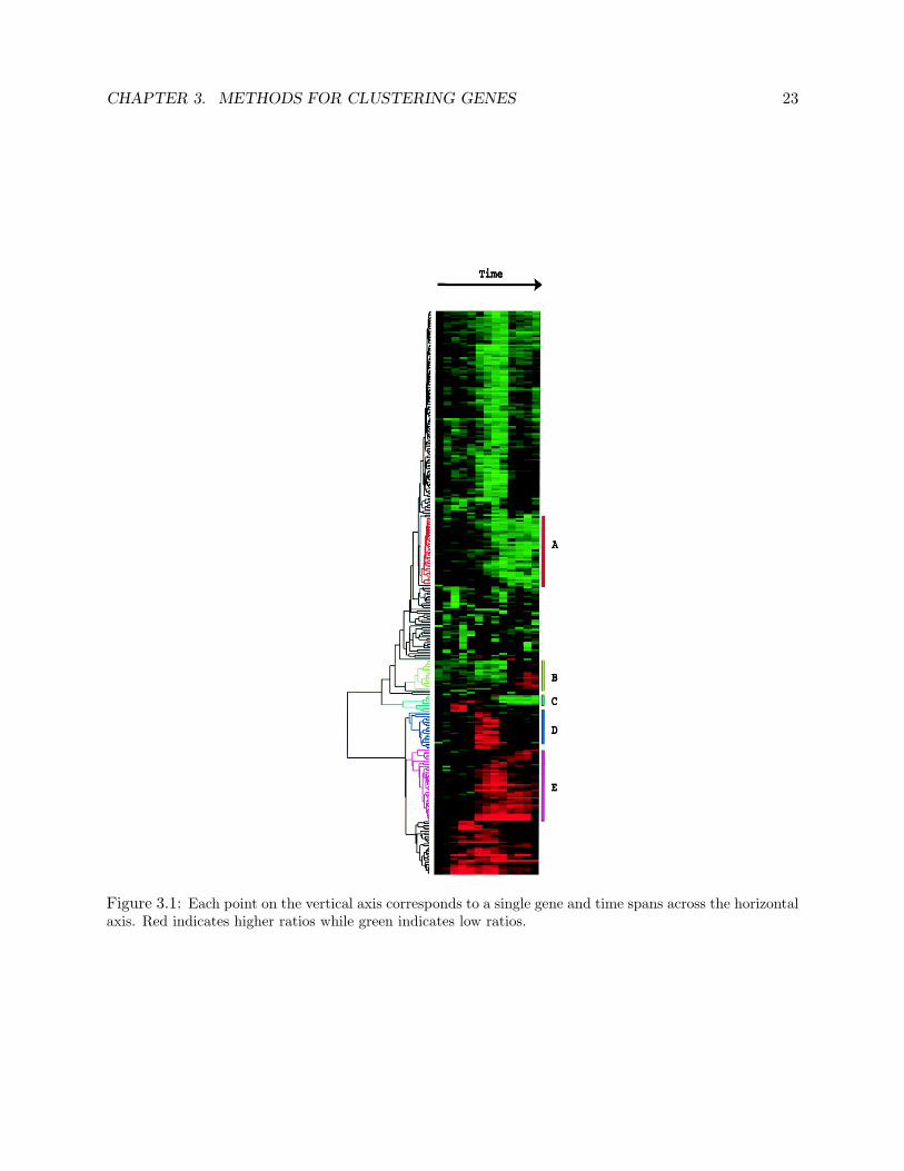
lengths reflect the degree of similarity between the objects. Figure 3.1 shows the visualization of
clusters (after reordering) and the corresponding dendrogram as presented in Eisen et al. (1998).
While correlation analysis is able to identify major clusters in the data, the major drawback of
this method is the disregarding of temporal dependencies. A complete understanding of the genetic
regulatory network is not complete without understanding the causal relationships in regulation.
Hence, it is of our opinion that correlation analysis is limited to identifying clusters of genes. Even
for this solution, one needs to identify the point at which the dendrogram is to be severed to obtain
cluster labels, which can be a difficult problem in an unsupervised setting such as theirs.
3.2 Statistical approaches to cluster time series data
Statistical approaches to cluster time series use statistical models like mixture models, hidden
Markov models (HMM), autoregressive models and the like. The primary use of these models is to
factor in the time dimension. We give a brief description of some of the statistical methods that
have been used to solve this problem.
3.2.1 CAGED - Cluster analysis of gene expression dynamics
Ramoni et al. (2002) applied a Bayesian method for model-based clustering of gene expression
time-course data (which they refer to as gene dynamics). Their method represents gene dynamics
CHAPTER 3. METHODS FOR CLUSTERING GENES 23
Figure 3.1: Each point on the vertical axis corresponds to a single gene and time spans across the horizontalaxis. Red indicates higher ratios while green indicates low ratios.
CHAPTER 3. METHODS FOR CLUSTERING GENES 24
in the form of autoregressive equations, and use an agglomerative procedure to search the most
probable partitioning of the data. The set of gene expression time-courses is supposed to have come
about from an unknown number of stochastic processes. The task is then to iteratively merge time
series into clusters, such that time series in a single cluster are generated by the same process. I
briefly give an outline of the components that constitute CAGED.
1. Autoregressive models - Gene time-courses are cast in pth order autoregressive framework,
where p specifies the the number of previous time steps that a single time step depends on.
For example, if p = 2, then the observation at time step i, yi, depends on yi−1 and yi−2. The
formulation also consists of an ‘error’ component, which is Gaussian distributed with mean
0. This can be thought of as the noise component.
2. Probabilistic scoring metric - A set of c clusters of time series is described as a statistical
model, Mc, consisting of c autoregressive models with coefficients and variance (of error).
The posterior probability of the model is given by
P (Mc|y) = P (Mc)f(y|Mc) (3.3)
where y is the data and f(y|Mc) is the likelihood function. Assuming a uniform prior over
the model, the posterior depends only on the likelihood factor, and this factor is used as the
probabilistic scoring metric.
3. Agglomerative Bayesian Clustering - An agglomerative, finite-horizon search strategy that
iteratively merges time series into clusters is then applied. The procedure starts by assuming
that each of the m observed time series is generated by a different process. The initial model,
Mm, consists of m clusters, one for each time series, with score f(y|Mm). The next step is the
computation of the marginal likelihood of the m(m− 1) models in which two of the m series
are merged into one cluster. The model Mm−1 with maximal marginal likelihood is chosen. If
f(y|Mm) ≥ f(y|Mm−1) then no merging is accepted and the procedure stops. Else, two time
series are merged into one cluster and the procedure repeats until no acceptable merging is
found.

CHAPTER 3. METHODS FOR CLUSTERING GENES 25
4. Heuristic search - The computational cost of the agglomerative clustering can be very high, in
particular if the number of time-courses is large, then the merging procedure starts with that
many initial clusters. In order to address this issue, the authors apply a heuristic search to
find ‘similar’ clusters. Computing m(m− 1) similarity scores is more feasible than the earlier
method of merging and computing likelihood. The intuition behind this being, similar clusters
when merged are more likely to increase the marginal likelihood. The heuristics they apply
to compute similarity is Euclidean distance (other metrics like correlation, Kullback-Leibler
divergence can be applied as well). Once the merging of time series is done, the average profile
of the cluster is computed by averaging over the two time series. Here again, the merging
stops when no acceptable merging (that which increases the marginal likelihood) is found.
CAGED seems to be a simple and intuitive method to cluster gene expression time-courses.
The authors have done an extensive comparison of the results obtained by CAGED to correlation
analysis of Eisen et al. (1998). While the latter method identifies 8 clusters, CAGED identifies
4 clusters. CAGED, though simple, I believe, is not free from drawbacks. The heuristic search
procedure does not completely alleviate the computational burden - once similar clusters have
been found, the marginal likelihood still has to be calculated to see verify if merging will increase
likelihood. It is not entirely clear how the ‘average profile’ is computed. A simple average of the
constituting time series may not be the most principled way of averaging time series. Lastly, the
number of time steps in each time-course could pose a problem. Autoregression may not perform
as well as some other time-series models for long time series.
3.2.2 Finite HMM with Gaussian output
Since the data is a time series data, use of a traditional time series modeling technique like HMM
makes sense. One of the most recent approaches to apply HMM to gene data in time-course was
by Schliep et al. (2005). The authors have used mixtures of HMM and model collection techniques
for the task. A brief description of their method is given below.
Their method consists of four major building blocks: First, hidden Markov models - to cap-
ture qualitative behavior of time-courses. Second, initial model collection (can be arrived at by
various methods). Third, estimation of a finite mixture model using prior information in a par-
CHAPTER 3. METHODS FOR CLUSTERING GENES 26
tially supervised clustering setting. Fourth, inferring groups from the mixture using entropy and
thresholding.
Hidden Markov models have been used with great success for time series applications such as
Part-of-Speech taggers, speech recognition, stock market analysis etc. Refer to Juang and Rabiner
(1991) for a good overview of HMM and one of its applications. The principle behind HMM is
that the observed sequence (in time) is a caused by a hidden sequence. The hidden sequence is a
first order Markov chain (higher orders are possible as well) - where the hidden state at time i, vi,
depends only on the hidden state at time i− 1, vi−1. The number of hidden states is fixed before
the model is learnt, and is usually done by trial-and-error or a model selection technique like Akaike
Information criterion (AIC) or Bayesian Information criterion (BIC).
The algorithm used by Schliep et al. (2005) starts off with an initial collection of k HMMs.
This collection is obtained in one of the three ways: First, expert selection - in which an expert
hand-crafts the models. Alternatively, one can start with an exhaustive collection of models encod-
ing all prototypical methods. Second, randomized model collection. The authors suggest creating
k different N state HMM with identical Gaussian emissions centered around zero. After which
Baum-Welch training is performed until convergence with each of the k models. Then the gene ex-
pression time-courses are weighted with random, uniform in [0, 1] weights per model. The resulting
randomized model collection would explain random sub-populations of the data. Third, a Bayesian
model collection technique based on Bayesian model merging by Stolcke and Omohundro (1993)
is suggested as a technique to learn the initial collection. Here the states of k N -state HMM are
first merged within HMM by identifying successive states whose merging decreases the likelihood
the least. This kind of horizontal merging continues until an expert/user given input N0 states per
HMM is reached. After which, merging of states across the k HMM takes place, again the criterion
for merging being minimal loss of likelihood.
This step is then followed by formulating the whole problem as a mixture of HMMs, whose
nonstatistical analogue is fuzzy clustering. Here, all the k HMMs share responsibility for every
time-course and the sum of responsibilities sum to 1. Thus k linear HMMs are combined to
one probability density function. This mixture model can be optimized with the Expectation
Maximization (Dempster et al. (1977)) algorithm to compute the maximum likelihood estimates.
CHAPTER 3. METHODS FOR CLUSTERING GENES 27
The authors also suggest a partially supervised learning extension to the standard EM algorithm.
For inference and assignment of gene time-courses to clusters, entropy criterion is used. Each
gene time-course is assigned to the cluster of maximal posterior, however to be more accurate with
assignments, this step is preceded by a computation of the entropy over the mixture probabilities.
If the entropy is below a certain user defined threshold, then such an assignment is carried out, else
the gene is assigned to a different ‘anonymous’ cluster. The computation of entropy can be seen as
the evaluation of ambiguity in cluster assignment.
This algorithm has been applied to two real gene expression time course data sets and two
simulated data sets. Though the results look good, there are a number of places where expert
input/intervention is required in this procedure. Below, we note some of the shortcomings of their
method.
1. The number of HMMs k in the mixture need to be fixed. The authors have suggested a BIC
method to estimate the number of components in the mixture, but BIC is not without its
problems. It can over or underestimate the number of true components.
2. In the Bayesian model collection technique, the number of states at which merging should
stop is defined by the user/expert. Again, not something desirable.
3. The entropy threshold used in the inference step is also user input. Fixing entropy threshold
(even aided by a visual interface as mentioned in the paper) is not the best way of fixing
thresholds and at best captures the intuition of the user.
3.2.3 Other approaches
Among the other popular approaches that have been tried to model gene expression time-course
data are piecewise polynomial curve fitting. We briefly discuss the idea given by Bar-Joseph et al.
(2003). In the algorithm proposed by the authors, each expression profile is modeled as a cubic spline
(piecewise polynomial) that is estimated from the observed data and every time point influences the
overall smooth expression curve. They constrain the spline coefficients of genes in the same class
to have similar expression patterns, while also allowing gene specific parameters. Their algorithm
attempts to address three different problems which appear commonly in gene expression analysis
CHAPTER 3. METHODS FOR CLUSTERING GENES 28
- missing value estimation, clustering and alignment. Missing value estimation can be performed
only after the spline coefficients are known, hence the first task is to get an estimate of the spline
coefficients. The authors present an algorithm called ‘TimeFit’ to estimate the spline coefficients
and obtain clusters simultaneously. In brief, the algorithm takes the number of clusters, c, as an
input and performs a modified EM (Dempster et al. (1977)). It starts of by assigning each class
a gene at random, and estimating the spline coefficients (with suitable allowance for noise). This
constitutes the E step. The M step maximizes the parameters for each class with respect to the
class probability (as computed in the E step). We notice that this algorithm closely resembles
the k-means algorithm we have seen earlier. They share the same drawbacks as well. Mainly, the
number of clusters, c, needs to be given as an input, and secondly EM converges to a local minima,
which means that initialization plays an important role in the clustering result.
In this chapter we have seen the different approaches researchers have taken towards clustering
gene expression time-course data. In the next chapter we see the approach we propose. Since
it’s a novel method and is an application of the Hierarchical Dirichlet Process, introduced by Teh
et al. (2004), a good part of the chapter is devoted to the explanation of Dirichlet Processes (DP)
(Ferguson (1973)) and Hierarchical Dirichlet Processes (HDP). Parts of this chapter have been
taken from Teh et al. (2004), Teh et al. (2006), and my colleague, Rahul Krishna’s notes on DP,
HDP, and their applications.
Chapter 4
The infinite hidden Markov model
Consider a situation which involves separation of data into groups, such that each data point is a
draw from a mixture model but we also have the requirement that mixture components be shared
across groups. This requirement is different from an ordinary mixture model (like a Gaussian
mixture model) where each component has a ‘responsibility’ factor in producing each data point.
Here, each group of data has its own mixture model and some of the components are common to
two or more groups. Such a scenario lends itself naturally to hierarchical modeling - parameters
are shared among different groups, and the randomness of the parameters induces dependencies
among the groups. For example: Consider a problem from the field of Information Retrieval (IR).
In document modeling, the occurrence of words in a document are considered to be conditionally
independent of each other (Salton and McGill (1983)), conditioned on a ‘topic’ (analogous to a
cluster). And each topic is modeled as a distribution over words from a vocabulary (Blei et al.
(2003)). As an example, consider a document which talks of university funding. The words in
this document might be drawn from topics like ‘education’ and ‘finance’. If this document were
a part of a corpus which also has other documents, say, one of which talks of university football,
then the topics for this document may be ‘education’ and ‘sports’. Thus we see that topics (or
clusters) are shared across different groups of data (documents). The topic ‘education’ is shared
among many different documents, and each document has its words drawn from several topics (one
of which could be ‘education’). As we shall see, the Hierarchical Dirichlet Process aims to solve
such clustering problems.
29

CHAPTER 4. THE INFINITE HIDDEN MARKOV MODEL 30
Hierarchical Dirichlet Processes (HDP) was introduced by Teh et al. (2004), and is a non-
parametric approach to model-based clustering. The data is divided into a set of J groups, and
the task is to find clusters within each group which capture the latent structure of the data in the
group. The number of clusters within each group is unknown and is to be inferred from the data.
Moreover, the clusters need to be shared across groups.
As a build-up to the HDP and Hierarchical Dirichlet Processes - Hidden Markov Model (HDP-
HMM), which is our approach to clustering gene expression time-course data, we’ll see Dirichlet
Processes (DP) and some of its characterizations which will help us better understand HDP and
HDP-HMM.
4.1 Notation
Before we go into the detail of DP and HDP, lets make explicit the notation we will be following
in this chapter. The data points or observations are organized into groups and observations are
assumed to be exchangeable within groups. In particular, let j ∈ {1, 2, . . . J} be the index for J
groups of data. Let xj = (xji)nj
i=1 denote the nj observations in group j. We assume that each
observation xji is conditionally independent draw from a mixture model, where the parameters of
the mixture model are drawn once per group. We also assume that x1,x2, . . .xJ are exchangeable
at the group level. Let x = (xj)Jj=1 denote the entire data set.
If each observation is drawn independently from a mixture model, then there is a mixture
component associated with each observation. Let θji denote a parameter specifying the mixture
component associated with observation xji. These θji are also referred to as factors, and in general
factors need not be distinct. Let F (θji) denote the distribution of xji given the factor θji. Let Gj
denote the prior distribution for the factors θj = (θji)nj
i=1 associated with the group j. Thus we
have the following model:
θji | Gj ∼ Gj for each j and i (4.1)
xji | θj ∼ F (θji) for each j and i (4.2)

CHAPTER 4. THE INFINITE HIDDEN MARKOV MODEL 31
In the next section, when we talk about Dirichlet Processes, we deal only with one group of
data, hence the subscript denoting group will be dropped as needed.
4.2 Dirichlet Processes
The Dirichlet Process, DP (α, G0), is a measure on measures. It has two parameters, a scaling
parameter α > 0 and a base measure G0. Ferguson (1973) defined DP as follows:
Definition 1: Let Θ be a continuous random variable, G0 be a non-atomic probability
distribution on Θ, and α be a positive scalar. Let G be a random variable denoting a probability
distribution on Θ. We say that G is distributed by a Dirichlet Process with parameters α and G0
if for all natural numbers, k, and k-partitions, B, on Θ,
(G(Θ ∈ B1), G(Θ ∈ B2), . . . , G(Θ ∈ Bk)) ∼ Dir(αG0(B1), αG0(B2), . . . , αG0(Bk)) (4.3)
Here, G(Θ ∈ Bi) is the probability of Θ ∈ Bi under the probability distribution G. Thus,
G(Θ ∈ Bi) = P (Θ ∈ Bi|G)
It can be noted that the Dirichlet distribution is a special case of the Dirichlet Process where
Θ is finite and discrete.
We write G ∼ DP (α,G0) if G is a random probability measure with distribution given by the
Dirichlet Process.
Readers interested in foundations (definitions, theorems and proofs) of Dirichlet process may
refer to Appendix A.
4.2.1 The Polya urn scheme and the Chinese restaurant process
The marginal probability of Θ ∈ Bi under the posterior is given by (A.8). The Polya urn model
(Blackwell and MacQueen (1973)) gives another perspective of the Dirichlet process. It refers to
draws from G. Consider a sequence of independently and identically distributed (i.i.d.) samples
θ1, θ2, . . . , θn, distributed according to G. Blackwell and MacQueen (1973) showed that the proba-
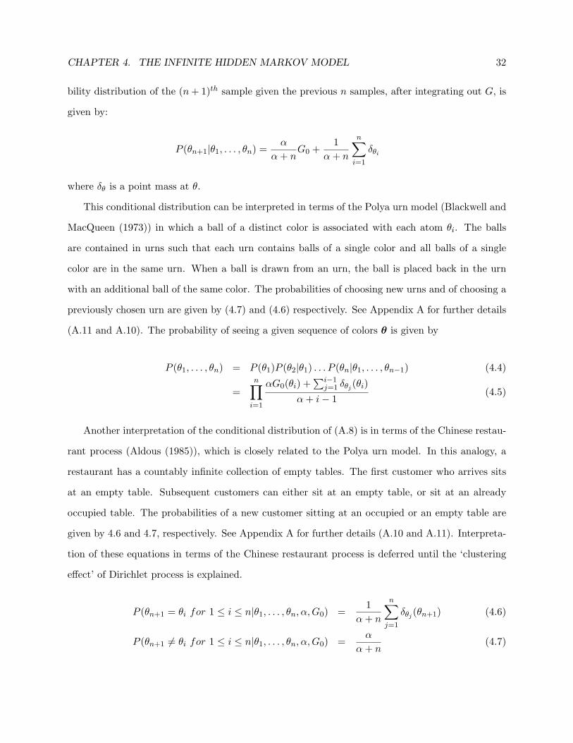
CHAPTER 4. THE INFINITE HIDDEN MARKOV MODEL 32
bility distribution of the (n+ 1)th sample given the previous n samples, after integrating out G, is
given by:
P (θn+1|θ1, . . . , θn) =α
α+ nG0 +
1α+ n
n∑i=1
δθi
where δθ is a point mass at θ.
This conditional distribution can be interpreted in terms of the Polya urn model (Blackwell and
MacQueen (1973)) in which a ball of a distinct color is associated with each atom θi. The balls
are contained in urns such that each urn contains balls of a single color and all balls of a single
color are in the same urn. When a ball is drawn from an urn, the ball is placed back in the urn
with an additional ball of the same color. The probabilities of choosing new urns and of choosing a
previously chosen urn are given by (4.7) and (4.6) respectively. See Appendix A for further details
(A.11 and A.10). The probability of seeing a given sequence of colors θ is given by
P (θ1, . . . , θn) = P (θ1)P (θ2|θ1) . . . P (θn|θ1, . . . , θn−1) (4.4)
=n∏i=1
αG0(θi) +∑i−1
j=1 δθj(θi)
α+ i− 1(4.5)
Another interpretation of the conditional distribution of (A.8) is in terms of the Chinese restau-
rant process (Aldous (1985)), which is closely related to the Polya urn model. In this analogy, a
restaurant has a countably infinite collection of empty tables. The first customer who arrives sits
at an empty table. Subsequent customers can either sit at an empty table, or sit at an already
occupied table. The probabilities of a new customer sitting at an occupied or an empty table are
given by 4.6 and 4.7, respectively. See Appendix A for further details (A.10 and A.11). Interpreta-
tion of these equations in terms of the Chinese restaurant process is deferred until the ‘clustering
effect’ of Dirichlet process is explained.
P (θn+1 = θi for 1 ≤ i ≤ n|θ1, . . . , θn, α,G0) =1
α+ n
n∑j=1
δθj(θn+1) (4.6)
P (θn+1 6= θi for 1 ≤ i ≤ n|θ1, . . . , θn, α,G0) =α
α+ n(4.7)

CHAPTER 4. THE INFINITE HIDDEN MARKOV MODEL 33
θ2
1
6
4
3 5
8
7321 4φ
θθθ φ θ φ
θθ φ
θ
Figure 4.1: A depiction of the Chinese restaurant after eight customers have been seated. Customers(θi’s) are seated at tables (circles) which correspond to unique values φk.
Above equations show the ‘clustering effect’ of DPs. This clustering property exhibited from
the conditional distributions can be made more explicit by introducing a new set of variables that
represent the distinct values of the atoms. We define φ1, . . . , φK to be the distinct values taken
by θ1, . . . , θn, and mk to be the number of values of θi′ that are equal to φk, 1 ≤ i′ ≤ n. We can
re-write (A.8) as
P (θn+1|θ1, . . . , θn) =α
α+ nG0 +
K∑k=1
mk
α+ nδφk
(4.8)
Thus, with respect to the Chinese restaurant process analogy, the customers are θi’s and the
tables are φk’s. Figure 4.1 depicts the Chinese restaurant process. We can observe from (4.8)
above, that the probability of a new customer occupying an empty table is proportional to α and
the probability of a new customer occupying an occupied table is proportional to the number of
customers already at that table. By drawing from a Dirichlet process, a partitioning of Θ is induced,
and the Chinese restaurant process and the Polya urn model define the corresponding distribution
over these partitions.
We can observe from (4.4) and (4.5) above that the ordering of θ’s does not matter. Thus the
Polya Urn model and the Chinese restaurant process yield exchangeable distributions on partitions.
From the definition of exchangeability (see Appendix A), it is reasonable to act as if there is
an underlying parameter and a prior on that parameter, and that the data are conditionally i.i.d.
given that parameter. This justifies the graphical model for a Dirichlet process is given in Figure
4.2. Here, G, the draw from a Dirichlet process, can be considered such a parameter.
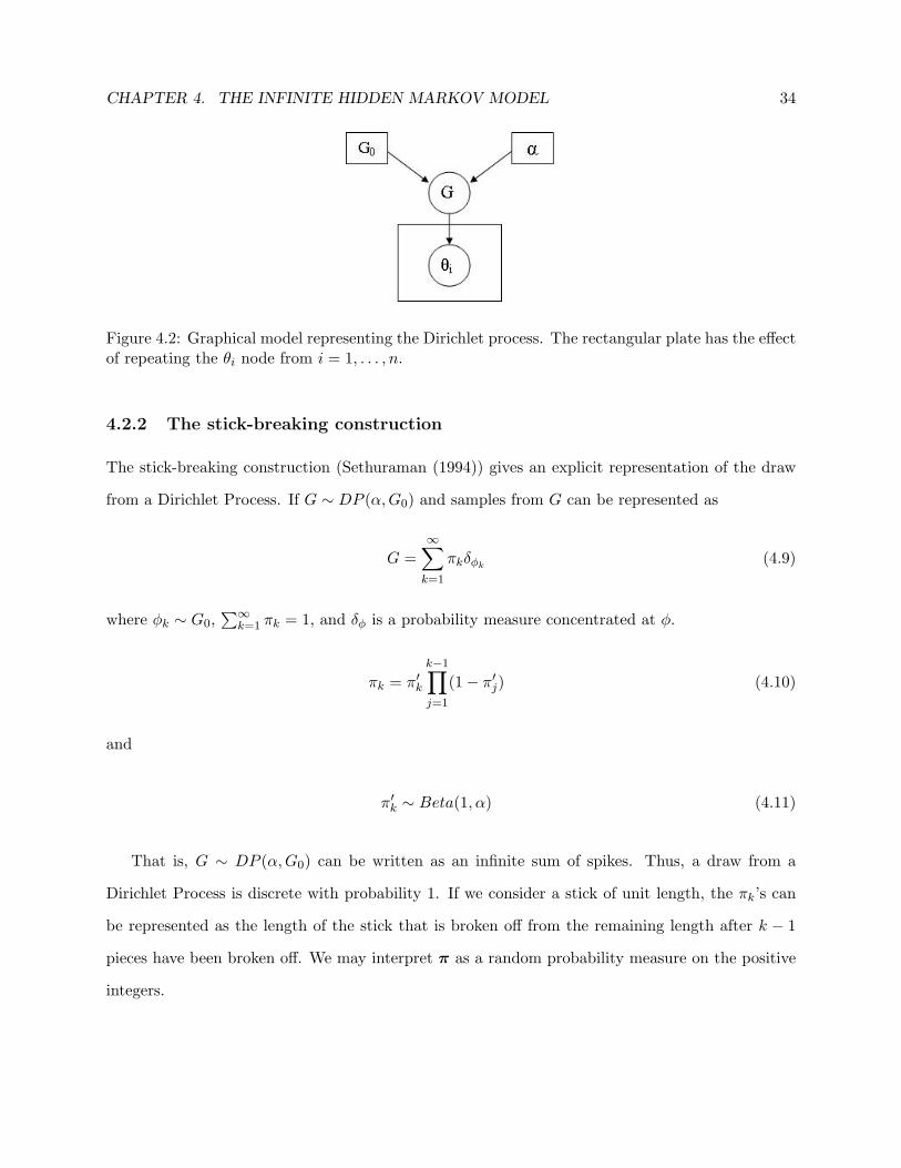
CHAPTER 4. THE INFINITE HIDDEN MARKOV MODEL 34
Figure 4.2: Graphical model representing the Dirichlet process. The rectangular plate has the effectof repeating the θi node from i = 1, . . . , n.
4.2.2 The stick-breaking construction
The stick-breaking construction (Sethuraman (1994)) gives an explicit representation of the draw
from a Dirichlet Process. If G ∼ DP (α,G0) and samples from G can be represented as
G =∞∑k=1
πkδφk(4.9)
where φk ∼ G0,∑∞
k=1 πk = 1, and δφ is a probability measure concentrated at φ.
πk = π′k
k−1∏j=1
(1− π′j) (4.10)
and
π′k ∼ Beta(1, α) (4.11)
That is, G ∼ DP (α,G0) can be written as an infinite sum of spikes. Thus, a draw from a
Dirichlet Process is discrete with probability 1. If we consider a stick of unit length, the πk’s can
be represented as the length of the stick that is broken off from the remaining length after k − 1
pieces have been broken off. We may interpret π as a random probability measure on the positive
integers.

CHAPTER 4. THE INFINITE HIDDEN MARKOV MODEL 35
θ
0α G
i
xin
0G
Figure 4.3: Graphical model representing the Dirichlet process mixture model
4.2.3 Dirichlet process mixture model
An important application of the Dirichlet Process is the Dirichlet Process mixture model. Here, a
Dirichlet Process is used as a non-parametric prior on the parameters of a mixture model. Let xi
be the observations that arise as follows:
θi|G ∼ G (4.12)
xi|θi ∼ F (θi) (4.13)
where F (θi) denotes the distribution of the observations given θi. When G is distributed according
to a Dirichlet Process, this models is referred to as a Dirichlet Process mixture model. A graphical
model representation of the Dirichlet Process mixture model is given in Figure 4.3.
In terms of the Chinese Restaurant Process, the customers are the θi’s and sit at tables that
represent the parameters of the distribution F (θi). For example, in the case that F (.) is a Normal
distribution, θi would be the (µ, σ) pairs. The prior distribution over θi is given by G. A new
customer either samples a new θ (i.e. an unoccupied table) or joins in with an already sampled θ.
The distribution over which table θi joins, given the previous samples, is given by the conditional
distributions governing the Chinese restaurant process.

CHAPTER 4. THE INFINITE HIDDEN MARKOV MODEL 36
In terms of the stick-breaking construction, the θi’s take on values φk with probability πk.
We can indicate this using an indicator variable zi, which specifies the ‘cluster number’ of each
observed datapoint xi. Hence we have the stick-breaking representation of the Dirichlet Process
mixture model as:
πk|α ∼ βk
k−1∏j=1
(1− βj)
zi|π ∼ π
φk|G0 ∼ G0
xi|zi, (φk)∞k=1 ∼ F (φzi)
where G =∑∞
k=1 πkδφkand θi = φzi .
4.3 Hierarchical Dirichlet processes
The Hierarchical Dirichlet Process (Teh et al. (2006)) has been used for the modeling of grouped
data, where each group is associated with a mixture model, and where it is desired to link these
mixture models by sharing mixture components between groups. A Hierarchical Dirichlet Process
is a distribution over a set of random probability measures over Θ. The process defines a set of
random probability measures (Gj)Jj=1, one for each group, and a global random probability measure
G0. The global measure G0 is distributed as a Dirichlet Process with concentration parameter γ
and base probability measure H:
G0|γ,H ∼ DP (γ, H)
The random probability measures Gj are conditionally independent given G0, and are distributed
as:
Gj |α,G0 ∼ DP (α, G0)

CHAPTER 4. THE INFINITE HIDDEN MARKOV MODEL 37
Each of the priors Gj are used as priors on the parameters of the mixture model for the jth group.
That is:
θji|Gj ∼ Gj
xji|θji ∼ F (θji)
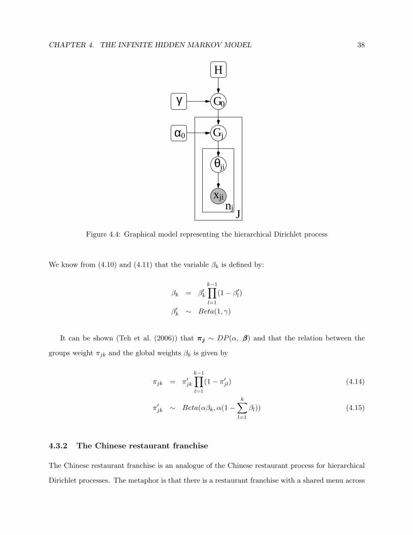
The graphical model is shown in 4.4
It is important to note that G0 is a draw from a Dirichlet Process. Supposing instead that each
of the Gj ’s are drawn from a single underlying Dirichlet Process DP (α,G0(τ)), where G0(τ) is a
parametric distribution with random parameter τ , there would be no sharing possible. This is due to
the fact that even though the samples from each of the Gj ’s are discrete, they would have no atoms
in common as the common base measure G0(τ) is continuous. That is P (θj1a = φk, θj2b = φk) = 0.
This can be avoided by using a discrete distribution G0 as the base measure, but this would no
longer yield flexible models. By making G0 a draw from a Dirichlet process, G0 ∼ DP (γ,H) is
discrete and yet has broad support, and necessarily, each of the Gj ’s has support at the same points
and hence sharing is possible.
4.3.1 The stick-breaking construction
The global measure G0 for the groups is distributed as a Dirichlet Process, and using the stick
breaking representation, we can write:
G0 =∞∑k=1
βkδφk
Since G0 has support at the points φ = (φk)∞k=1, each Gj necessarily has support over these points
as well and thus:
Gj =∞∑k=1
πjkδφk,
CHAPTER 4. THE INFINITE HIDDEN MARKOV MODEL 38
θ
Gj
γ G0
H
0α
xjinj
J
ji
Figure 4.4: Graphical model representing the hierarchical Dirichlet process
We know from (4.10) and (4.11) that the variable βk is defined by:
βk = β′k
k−1∏l=1
(1− β′l)
β′k ∼ Beta(1, γ)
It can be shown (Teh et al. (2006)) that πj ∼ DP (α, βββ) and that the relation between the
groups weight πjk and the global weights βk is given by
πjk = π′jk
k−1∏l=1
(1− π′jl) (4.14)
π′jk ∼ Beta(αβk, α(1−k∑l=1
βl)) (4.15)
4.3.2 The Chinese restaurant franchise
The Chinese restaurant franchise is an analogue of the Chinese restaurant process for hierarchical
Dirichlet processes. The metaphor is that there is a restaurant franchise with a shared menu across
CHAPTER 4. THE INFINITE HIDDEN MARKOV MODEL 39
j
β
kφ
H
8
γ
0α
z
π
ji
xjinj
J
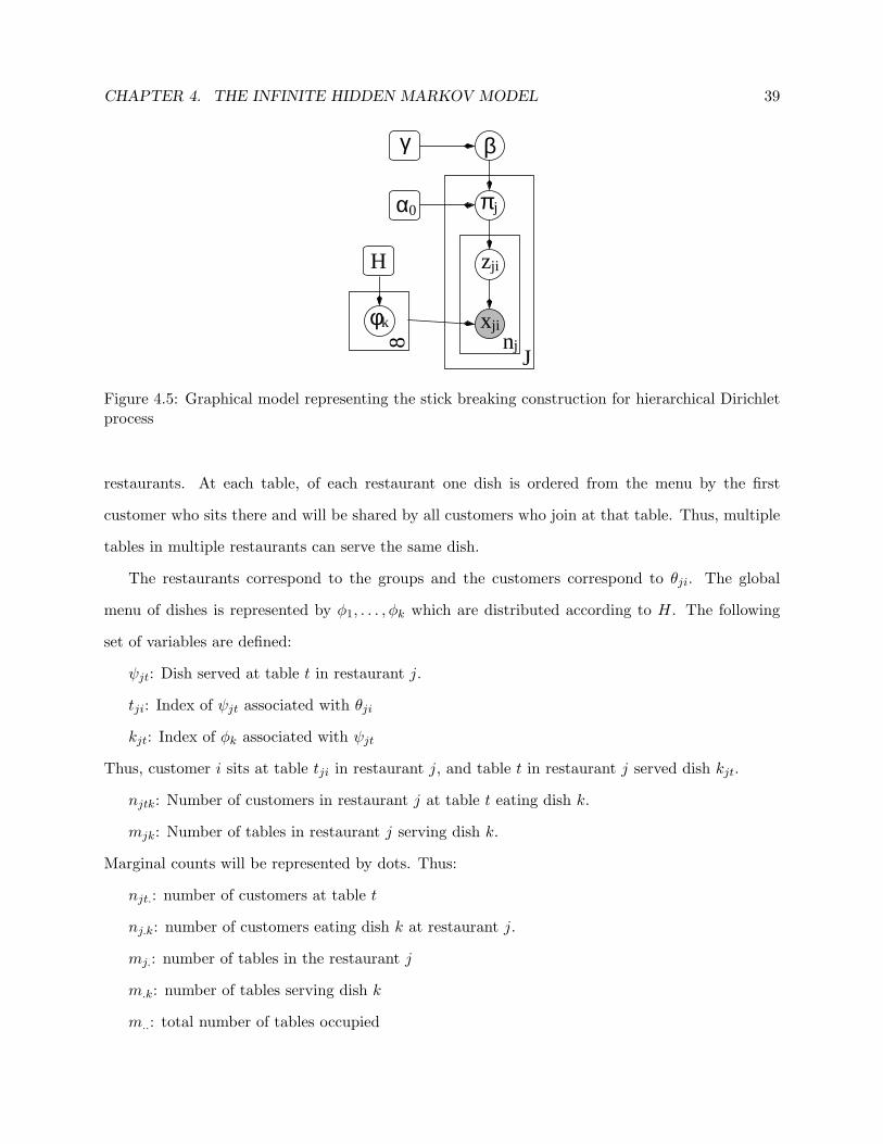
Figure 4.5: Graphical model representing the stick breaking construction for hierarchical Dirichletprocess
restaurants. At each table, of each restaurant one dish is ordered from the menu by the first
customer who sits there and will be shared by all customers who join at that table. Thus, multiple
tables in multiple restaurants can serve the same dish.
The restaurants correspond to the groups and the customers correspond to θji. The global
menu of dishes is represented by φ1, . . . , φk which are distributed according to H. The following
set of variables are defined:
ψjt: Dish served at table t in restaurant j.
tji: Index of ψjt associated with θji
kjt: Index of φk associated with ψjt
Thus, customer i sits at table tji in restaurant j, and table t in restaurant j served dish kjt.
njtk: Number of customers in restaurant j at table t eating dish k.
mjk: Number of tables in restaurant j serving dish k.
Marginal counts will be represented by dots. Thus:
njt.: number of customers at table t
nj.k: number of customers eating dish k at restaurant j.
mj.: number of tables in the restaurant j
m.k: number of tables serving dish k
m..: total number of tables occupied
CHAPTER 4. THE INFINITE HIDDEN MARKOV MODEL 40
We can write the conditional probabilities of θji given the previous i− 1 samples at restaurant
j and 0 by integrating out Gj . From (4.8),
θji|θj1, . . . , θj,i−1, α,G0 ∼mj∑t=1
njt.α+ i− 1
δψjt+
α
α+ i− 1G0 (4.16)
Next, by integrating out G0, we can compute the conditional distribution of ψjt as:
ψjt|ψ11, ψ12, . . . , ψ21, . . . , ψj,t−1, γ,H ∼K∑k=1
m.k
m.. + γδφk
+γ
m.. + γH (4.17)
where K is the total number of dishes.
4.4 The infinite hidden Markov model
4.4.1 Hidden Markov models
Hidden Markov models (HMM) are a popular statistical model used to model time series data. They
have found wide usage in speech recognition, natural language processing, information retrieval, and
other time series data applications like stock market prediction. Early HMM theory was developed
by Baum and Petrie (1966) and Baum et al. (1970). A HMM models a sequence of observations
y1:T = {y1, . . . , yT } by assuming that the observation at time t, yt, was produced by a hidden state
vt, and the sequence of hidden states v1:T = {v1, . . . , vT } was generated by a first-order Markov
process. The complete data likelihood of the sequence, of length T, is given by:
p(v1:T ,y1:T ) = p(v1)p(y1|v1)T∏t=2
p(vt|vt−1)p(yt|vt) (4.18)
where p(v1) is the initial probability of first hidden state, p(vt|vt−1) is the transition probability
going from vt−1 to vt, and p(yt|vt) is the probability of ‘emitting’ the observable yt while in hidden
state vt. For a simple HMM, it is assumed that there are a fixed number of hidden states (say
‘k’) and a fixed number of observable symbols (say ‘p’) and that the transition probabilities are
stationary. With these assumptions, the parameter, θ, of the model comprises of the state transition

CHAPTER 4. THE INFINITE HIDDEN MARKOV MODEL 41
probabilities, A, the emission probabilities, C, and the initial state prior, π. That is:
θ = (A,C,π) (4.19)
where
A = {ajj′} : ajj′ = p(vt = j′|vt−1 = j) k x k state transition matrix (4.20)
C = {cjm} : cjm = p(yt = m|vt = j) k x p emission matrix (4.21)
π = {πj} : πj = p(v1 = j) k x 1 initial state vector (4.22)
obeying the normalization constraints:
A = {ajj′} :k∑
j‘=1
ajj′ = 1 ∀j (4.23)
C = {cjm} :p∑
m=1
cjm = 1 ∀j (4.24)
π = {πj} :k∑j=1
πj = 1 (4.25)
Parameter estimation in an HMM is done using the Baum-Welch algorithm (Baum et al. (1970)),
which is an EM algorithm used to find the ML estimate of the parameters. Briefly, the M step
consists of finding those settings of A, C and π which maximize the probability of the observed
data, and the E step (known as forward-backward algorithm for HMMs) amounts to calculating the
expected count of the particular transition-emission pair, employing a dynamic programming trick.
For more details on the Baum-Welch algorithm, refer to Baum et al. (1970).
4.4.2 HDP-HMM
To understand the hidden Markov model in the HDP framework, it is easier to view hidden Markov
model of the previous subsection in a different way than presented there, and then relate it to the
stick-breaking construction of section 4.3.1. The work here can be found in the HDP paper, which
interestingly was originally inspired by an infinite hidden Markov model paper by Beal et al. (2002).

CHAPTER 4. THE INFINITE HIDDEN MARKOV MODEL 42
A hidden Markov model is a doubly stochastic Markov chain in which a sequence of multinomial
‘state’ variables {v1, . . . , vT } are linked via a state transition matrix, and each element yt in a
sequence of ‘observations’ {y1, . . . , yT } is drawn independently of the other observations conditional
on vt (Rabiner (1989)). HMM is a dynamic variant of a finite mixture model, in which there is
one mixture component corresponding to each value of the multinomial state. Note that the HMM
involves not a single mixture model, but rather a set of mixture models: one for each value of the
current state. That is, the ‘current state’ vt indexes a specific row of the transition matrix, with the
probabilities in this row serving as the mixing proportions for the choice of the ‘next state’ vt+1.
Given the next state vt+1, the observation yt+1 is drawn from the mixture component indexed by
vt+1.
The stick breaking representation makes explicit the generation of one set of (countably infinite)
set of parameters (φk)∞k=1; the jth group has access to various of these parameters to model its
data (xji)nj
i=1, depending on the sampled mixing proportion πj .
Thus, to consider a nonparametric variant of the HMM which allows an unbounded set of states,
we must consider a set of DPs, one for each value of the current state. Moreover, these DPs must
be linked, because we want the same set of ‘next states’ to be reachable from each of the ‘current
states’. This amounts to the requirement that the atoms associated with the state-conditional DPs
should be shared—exactly the framework of the hierarchical DP. Thus, we simply replace the set
of conditional finite mixture models underlying the classical HMM with an HDP, and the resulting
model, an HDP-HMM, provides an alternative to methods that place an explicit parametric prior
on the number of states or make use of model selection methods to select a fixed number of states
(e.g. Stolcke and Omohundro (1993)).
Consider the unraveled hierarchical Dirichlet process representation shown in Figure 4.6. The
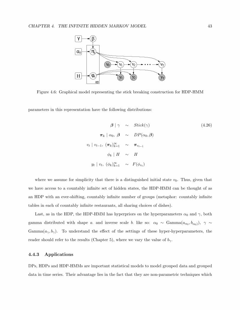
CHAPTER 4. THE INFINITE HIDDEN MARKOV MODEL 43
v1
γ β
kφH
kπ0α
v
2
2
y1
v0
8
vT
Tyy
Figure 4.6: Graphical model representing the stick breaking construction for HDP-HMM
parameters in this representation have the following distributions:
β | γ ∼ Stick(γ) (4.26)
πk | α0, β ∼ DP (α0,β)
vt | vt−1, (πk)∞k=1 ∼ πvt−1
φk | H ∼ H
yt | vt, (φk)∞k=1 ∼ F (φvt)
where we assume for simplicity that there is a distinguished initial state v0. Thus, given that
we have access to a countably infinite set of hidden states, the HDP-HMM can be thought of as
an HDP with an ever-shifting, countably infinite number of groups (metaphor: countably infinite
tables in each of countably infinite restaurants, all sharing choices of dishes).
Last, as in the HDP, the HDP-HMM has hyperpriors on the hyperparameters α0 and γ, both
gamma distributed with shape a· and inverse scale b· like so: α0 ∼ Gamma(aα0 , bα0)), γ ∼
Gamma(aγ , bγ). To understand the effect of the settings of these hyper-hyperparameters, the
reader should refer to the results (Chapter 5), where we vary the value of bγ .
4.4.3 Applications
DPs, HDPs and HDP-HMMs are important statistical models to model grouped data and grouped
data in time series. Their advantage lies in the fact that they are non-parametric techniques which

CHAPTER 4. THE INFINITE HIDDEN MARKOV MODEL 44
overcome the issue of fixing the model complexity prior to training. Some of the applications of
these tools include document modeling (see Teh et al. (2006)), time series data prediction (see Alice
in Wonderland example in Teh et al. (2006)), and clustering (next chapter). However, these models
do come at a cost - efficient sampling techniques are required for inference in these models (Markov
chain Monte Carlo schemes are used most often (see Neal (1998)). Finding efficient sampling
techniques still remains an important research area.

Chapter 5
Experiments
In this chapter, we present the results of clustering using HDP-HMM on two well known gene ex-
pression time course datasets - Yeast sporulation dataset (Cho et al. (1998)) and Human fibroblasts
dataset (Iyer et al. (1999)). Before we see the results, the datasets and the experimental set up are
described.
5.1 Datasets
1. Iyer dataset - Iyer et al. (1999) recorded the response of human fibroblasts to serum, using
cDNA microarrays representing about 8600 distinct human genes. Human fibroblasts require
growth factors for proliferation, usually provided by fetal bovine serum (FBS). In the absence
of growth factors, fibroblasts enter a state of low metabolic activity. Their study focused
on the observing the activity of human fibroblasts when simulated with 10% FBS, preceded
by 48 hours of serum deprivation. The expression levels of genes were measured at 12 times
ranging from 15 min to 24 hours.
The dataset used in our experiments consists of 517 genes across 12 time points. The ex-
pressions were log-normalized and standardized to have log expression 1 at time t = 1 for
all genes. The genes are labeled as belonging to a cluster 1-10, with an additional ‘outlier’
cluster (labeled -1). We believe that the labels for this dataset were obtained by correlation
analysis (Eisen et al. (1998)), followed by biology expert modification.
45

CHAPTER 5. EXPERIMENTS 46
2. Cho dataset - Cell cycle is the orderly sequence of events by which a cell duplicates its
contents and divides into two. It consists of mitosis (or division) and interphase. Cells
experience important physiological changes during the cell cycle, and diverse biological events
depend on maintenance of this periodicity. Loss of appropriate cell cycle regulation leads to
genomic instability (Hartwell and Kastan (1994)). The study conducted by Cho et al. (1998)
focuses on the mRNA transcript levels during the cell cycle of the budding yeast S.cerevisiae
of more than 6000 genes.
The data used in our experiments is a subset of this dataset, consisting of 386 genes’ expression
values across 17 time points. The genes are labeled as belonging to cluster 1-5. The data was
standardized prior to analysis.
5.2 Design
We compare our HDP-HMM to the standard hidden Markov model (with fixed number of hidden
states) - which we refer to as ‘finite HMM’. We also compare the HDP-HMM to the standard
correlation analysis. In correlation analysis, as seen in the Chapter 3, the dissimilarity between a
pair of genes is the inverse of correlation between the two time course ‘vectors’. Hence, we define
a similarity matrix, P, for the data as:
P = {pcd} : Corr(c, d) (5.1)
where Corr(c, d) is the correlation between the cth and the dth time courses (as given in Chapter
3). {−pcd} is used as the dissimilarity measure in a hierarchical agglomerative clustering procedure
to obtain a tree structure (more about the procedure later), which can be severed at a suitable
point to obtain a clustering of the data.
In the finite HMM case, we define the probabilistic similarity measure between two genes as
the probability that the time courses of each gene having identical hidden trajectories. This can be
easily computed after an E step in the Baum-Welch algorithm. Let the posterior over the hidden
state at time t of the cth gene sequence be p(v(c)t |y(c)
1:T ,Θ), where Θ are the current parameters of

CHAPTER 5. EXPERIMENTS 47
the HMM, then log Pcd is straightforwardly given by
T∑t=1
logk∑r=1
p(v(c)t = r|y(c)
1:T ,Θ)p(v(d)t = r|y(d)
1:T ,Θ) (5.2)
The quantity, Pcd, measures the probability of two genes, c and d, having traversed similar
hidden trajectories. Hence, - log Pcd is used as a measure of dissimilarity between genes c and d.
An analogous measure of similarity for HDP-HMM can be computed from the posterior distri-
bution over hidden state trajectories - which, in the case of an infinite model is a set of samples.
The similarity measure can be calculated simply from an empirical computation over the samples
of trajectories taken over very long MCMC runs. Despite the countably infinite state space of
HDP-HMM, the posterior samples always consist of represented hidden states, making this empir-
ical computation simple. A similar method is used in the (i.i.d.) clustering using infinite mixture
of Gaussians work of Rasmussen (2000) and Wild et al. (2002), but here we have extended to be a
measure of similarity over sequences.
Note that the metric computed by (5.2) is approximate in the sense that, by taking the product
of probabilities at each time point we are ‘discarding’ the temporal order - but the reader should
realize that the quantities which are being multiplied themselves are obtained considering the
temporal aspect of data. However, to go a step further and use the exact metric (as against
the approximate metric above), we also tried using the following formulation of Pcd (omitting the
subscript .1:T for brevity):
p(v(c) = v(d)|y(c),y(d)) =∑v
p(v(c) = v|y(c))p(v(d) = v|y(d)) (i.i.d)
=∑v
p(y(c)|v)p(v)p(y(c))
.p(y(d)|v)p(v)p(y(d))
=1
p(y(c))p(y(d))
∑v
p(y(c)|v)p(y(d)|v)p(v)2 (5.3)
The normalization factor (on the left hand side of the sum), in the above equation, can be
computed using the forward pass (one per observation sequence), while the expression within the
sum can be calculated by a simple modification to the forward pass, in which we perform a paired

CHAPTER 5. EXPERIMENTS 48
forward pass.
Once a dissimilarity measure matrix has been obtained from each of the above methods -
correlation, finite and infinite - the matrix is used in a hierarchical clustering procedure using
‘average’ linkage (see Chapter 2), to obtain a tree structure (called a dendrogram). The dendrogram
can be severed at a suitable point to get a set of C subtrees, and the leaves (time courses) of tree
are labeled such that all leaves in the same subtree belong to the same cluster. The dendrogram
also serves for visualization of the hierarchical clustering procedure.
5.3 Results
We compare the correlation analysis to finite HMMs with varying number of hidden states, k =
1, . . . , 40, and HDP-HMM with several settings of its hyper-hyperparameters. For finite HMM, we
ran experiments with 7 different seed values and averaged over the various scores. For HDP-HMM,
the auxiliary variable Gibbs sampling consisted of 100,000 burnin samples, collecting 250 posterior
samples thereafter having a spacing of 750 samples between each.
We present results in the form of tables, comparative plots of indices, and dendrograms. Most
of the results presented here pertain to the Cho dataset. The Cho dataset, apart from having
fewer genes, also has a fewer number of true clusters, which make it easy for visualization (in
dendrograms).
1. Set 1 (Table 5.1): This result shows the effect of varying the hyper-hyperparameter, bγ , setting
for the HDP-HMM for the Iyer dataset with varying values of C.
2. Set 2 (Figure 5.1): This set consists of plots of indices for correlation analysis, finite HMM
(all values of hidden states, k = 1, . . . , 40), and HDP-HMM (two values of the hyper-
hyperparameter - bγ = 1 and bγ = 3) for the Cho dataset.
3. Set 3 (Table 5.2): This set consists of index values in tabular form for both, Iyer and
Cho, datasets. The index values presented are for correlation analysis, finite HMM (k =
1, . . . , 40, both exact and finite methods of computing distances) and HDP-HMM (bγ =
0.25, 0.5, 1, 2, 3, 4, 5).

CHAPTER 5. EXPERIMENTS 49
(a) rand (b) jaccard (c) crand
(d) DB (e) silhouette (f) dunns
(g) purity (h) sens (i) spec
Figure 5.1: Comparative plot of indices with varying values of k for finite HMM, and two values of hyper-hyperparameter settings for HDP-HMM - with index values on y-axis and values of k along x-axis

CHAPTER 5. EXPERIMENTS 50
Table 5.1: Choice of number of clusters, C, for Iyer data.
rand crand jacc spec sensbγ =1, C=1 0.16 0.00 0.16 0.16 1.00
5 0.72 0.35 0.33 0.35 0.8910 0.73 0.36 0.34 0.36 0.8811 0.73 0.36 0.34 0.36 0.8815 0.80 0.41 0.36 0.42 0.7020 0.82 0.38 0.33 0.43 0.57
bγ =3, C=1 0.16 0.00 0.16 0.16 1.005 0.66 0.28 0.29 0.30 0.90
10 0.73 0.35 0.33 0.35 0.8311 0.75 0.36 0.33 0.36 0.8215 0.80 0.39 0.35 0.41 0.6920 0.80 0.39 0.35 0.42 0.67
4. Set 4 (Figures 5.2 and 5.3): This set consists of dendrograms for correlation analysis, finite
HMM (k = 5, 10, 20, 30, 40) and HDP-HMM (bγ = 0.25, 0.5, 1, 2, 3, 4).
5. Set 5 (Figure 5.4): This set consists of dendrograms for finite HMM, using the two methods
to compute probabilistic similarity metric, exact and approximate for values of k = 2, 5, 10.
5.4 Interpretation
As Table 5.1 shows, the effect of varying the hyper-hyperparameter setting, for the HDP-HMM,
is very small. This indicates that at this level of Bayesian hierarchy the settings of priors do not
influence the learning of the model significantly - as it should be. This is in contrast to the scores
obtained for finite HMM with varying values of k. In the latter case, we see that the scores vary
considerably when the number of hidden states varies - evident from Table 5.2 and Figure 5.1 (as
we scan across the x-axis). In other words, fixing the priors for a hierarchical non-parametric model
does not constrain the model - but only encapsulates our belief of the underlying distribution of
the data, as against a parametric model where it directly affects the learnt model.
From the plot of indices in Figure 5.1 it is clear that HDP-HMM performs as good as (and
better than, in most cases) finite HMM and correlation analysis. Also, finite HMM shows signs of
overfitting in crand and jaccard indices, when the scores taper down with increasing values of k.
Another trend we note is that correlation analysis performs well on external indices - agreement
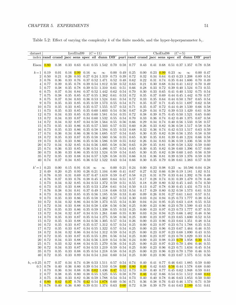
CHAPTER 5. EXPERIMENTS 51
Table 5.2: Effect of varying the complexity k of the finite models, and the hyper-hyperparameter bγ .
dataset IyerEtal99 (C =11) ChoEtal98 (C =5)index rand crand jacc sens spec sil dunn DB∗ puri rand crand jacc sens spec sil dunn DB∗ puri
Eisen 0.80 0.38 0.33 0.63 0.41 0.55 1.542 0.70 0.58 0.77 0.43 0.41 0.68 0.51 0.37 1.357 0.78 0.58
k=1 0.19 0.01 0.16 0.99 0.16 ∞ ∞ 0.00 0.49 0.25 0.00 0.23 0.99 0.23 ∞ ∞ 0.00 0.472 0.50 0.21 0.26 0.93 0.27 0.24 1.319 0.73 0.39 0.72 0.32 0.34 0.64 0.43 0.23 1.208 0.89 0.543 0.76 0.36 0.33 0.76 0.37 0.52 1.471 0.52 0.48 0.62 0.22 0.31 0.74 0.35 0.44 1.606 0.70 0.494 0.77 0.39 0.35 0.78 0.39 0.54 1.812 0.50 0.52 0.63 0.21 0.30 0.68 0.34 0.41 1.612 0.70 0.495 0.77 0.38 0.35 0.78 0.39 0.51 1.310 0.61 0.51 0.66 0.28 0.33 0.72 0.39 0.40 1.524 0.73 0.556 0.75 0.37 0.34 0.84 0.37 0.52 1.442 0.62 0.54 0.70 0.30 0.33 0.65 0.41 0.40 1.532 0.75 0.547 0.75 0.38 0.35 0.85 0.37 0.55 1.382 0.61 0.53 0.72 0.35 0.37 0.69 0.44 0.45 1.442 0.70 0.578 0.75 0.37 0.34 0.83 0.36 0.53 1.524 0.61 0.54 0.72 0.33 0.35 0.64 0.44 0.50 1.767 0.65 0.549 0.73 0.35 0.33 0.85 0.35 0.59 1.573 0.55 0.54 0.71 0.35 0.37 0.71 0.45 0.51 1.697 0.62 0.58
10 0.73 0.35 0.33 0.85 0.35 0.57 1.555 0.57 0.53 0.71 0.35 0.37 0.72 0.44 0.48 1.539 0.66 0.5811 0.73 0.35 0.33 0.85 0.35 0.60 1.603 0.54 0.56 0.67 0.29 0.34 0.72 0.39 0.53 1.429 0.61 0.5812 0.73 0.34 0.33 0.85 0.35 0.60 1.581 0.54 0.55 0.72 0.38 0.39 0.75 0.45 0.50 1.521 0.65 0.6013 0.72 0.34 0.33 0.87 0.34 0.60 1.532 0.55 0.54 0.70 0.33 0.36 0.74 0.42 0.48 1.375 0.67 0.5814 0.72 0.34 0.32 0.87 0.34 0.58 1.564 0.55 0.56 0.66 0.29 0.34 0.74 0.40 0.56 1.533 0.58 0.5715 0.73 0.35 0.33 0.86 0.35 0.57 1.503 0.57 0.55 0.60 0.26 0.33 0.82 0.36 0.58 1.517 0.58 0.5816 0.73 0.35 0.33 0.86 0.35 0.58 1.594 0.55 0.53 0.68 0.32 0.36 0.74 0.42 0.53 1.517 0.63 0.5917 0.74 0.36 0.34 0.86 0.36 0.56 1.685 0.57 0.54 0.65 0.30 0.35 0.82 0.38 0.56 1.355 0.58 0.5918 0.72 0.35 0.33 0.87 0.35 0.58 1.560 0.56 0.55 0.65 0.30 0.35 0.81 0.39 0.48 1.224 0.66 0.5819 0.73 0.35 0.33 0.86 0.35 0.56 1.586 0.59 0.55 0.62 0.26 0.34 0.83 0.36 0.59 1.336 0.56 0.5920 0.72 0.34 0.32 0.85 0.34 0.56 1.605 0.58 0.56 0.65 0.29 0.35 0.81 0.38 0.58 1.322 0.59 0.6025 0.74 0.36 0.33 0.85 0.36 0.54 1.486 0.57 0.54 0.65 0.30 0.35 0.82 0.38 0.60 1.396 0.57 0.6030 0.73 0.36 0.33 0.86 0.35 0.53 1.524 0.59 0.54 0.65 0.30 0.35 0.82 0.38 0.60 1.445 0.56 0.5935 0.72 0.35 0.33 0.88 0.34 0.57 1.528 0.58 0.55 0.66 0.31 0.36 0.81 0.39 0.59 1.376 0.59 0.5940 0.74 0.37 0.34 0.85 0.36 0.52 1.522 0.63 0.54 0.66 0.30 0.35 0.79 0.38 0.61 1.383 0.57 0.59
k′=1 0.23 0.00 0.15 0.91 0.16 ∞ ∞ 0.00 0.21 0.24 0.00 0.23 0.98 0.23 ∞ 10.586 0.04 0.282 0.49 0.20 0.25 0.93 0.26 0.21 1.104 0.80 0.41 0.67 0.27 0.32 0.66 0.38 0.19 1.181 1.02 0.513 0.76 0.33 0.31 0.69 0.37 0.47 1.619 0.59 0.47 0.58 0.21 0.31 0.79 0.33 0.44 1.392 0.76 0.484 0.76 0.37 0.33 0.76 0.38 0.45 1.603 0.64 0.51 0.57 0.17 0.28 0.74 0.31 0.39 1.479 0.78 0.465 0.73 0.34 0.32 0.85 0.34 0.53 1.372 0.59 0.51 0.55 0.18 0.29 0.80 0.32 0.45 1.445 0.74 0.506 0.73 0.35 0.33 0.88 0.35 0.53 1.258 0.61 0.54 0.50 0.13 0.27 0.78 0.30 0.45 1.431 0.73 0.517 0.76 0.38 0.34 0.81 0.37 0.49 1.118 0.68 0.53 0.54 0.17 0.29 0.80 0.32 0.58 1.573 0.61 0.538 0.73 0.34 0.33 0.85 0.35 0.56 1.185 0.58 0.53 0.40 0.09 0.26 0.91 0.27 0.61 1.641 0.57 0.519 0.73 0.35 0.33 0.86 0.35 0.58 1.362 0.57 0.53 0.30 0.03 0.24 0.94 0.25 0.73 1.777 0.38 0.54
10 0.72 0.34 0.32 0.86 0.34 0.58 1.373 0.55 0.54 0.30 0.04 0.24 0.95 0.25 0.63 1.418 0.55 0.5311 0.72 0.34 0.33 0.88 0.34 0.58 1.438 0.56 0.56 0.25 0.00 0.23 0.96 0.23 0.70 1.599 0.43 0.5312 0.73 0.35 0.33 0.86 0.35 0.59 1.338 0.55 0.53 0.25 0.00 0.23 0.97 0.23 0.73 1.777 0.37 0.5513 0.72 0.34 0.32 0.87 0.34 0.55 1.261 0.60 0.55 0.30 0.03 0.24 0.94 0.25 0.66 1.482 0.48 0.5614 0.73 0.35 0.33 0.87 0.35 0.54 1.275 0.58 0.56 0.25 0.00 0.23 0.97 0.23 0.65 1.600 0.52 0.5315 0.72 0.35 0.33 0.88 0.34 0.56 1.305 0.57 0.54 0.26 0.00 0.23 0.96 0.23 0.64 1.351 0.48 0.5416 0.72 0.35 0.33 0.87 0.35 0.57 1.312 0.57 0.54 0.25 0.00 0.23 0.97 0.23 0.74 1.788 0.35 0.5517 0.72 0.35 0.33 0.87 0.34 0.55 1.322 0.57 0.54 0.25 0.00 0.23 0.96 0.23 0.67 1.464 0.46 0.5518 0.72 0.34 0.32 0.86 0.34 0.54 1.312 0.59 0.54 0.25 0.00 0.23 0.97 0.23 0.68 1.890 0.43 0.5519 0.72 0.35 0.33 0.87 0.35 0.55 1.291 0.56 0.54 0.25 0.00 0.23 0.97 0.23 0.78 1.829 0.33 0.5420 0.72 0.34 0.33 0.88 0.34 0.56 1.319 0.54 0.56 0.24 0.00 0.23 0.98 0.23 0.79 1.958 0.30 0.5525 0.71 0.33 0.32 0.88 0.34 0.55 1.270 0.56 0.54 0.25 0.00 0.23 0.97 0.23 0.70 1.494 0.46 0.5530 0.72 0.34 0.33 0.87 0.34 0.53 1.219 0.59 0.54 0.25 0.00 0.23 0.96 0.23 0.71 1.634 0.45 0.5435 0.73 0.35 0.33 0.88 0.35 0.54 1.218 0.58 0.54 0.25 0.00 0.23 0.96 0.23 0.70 1.759 0.46 0.5540 0.72 0.35 0.33 0.89 0.34 0.54 1.244 0.60 0.54 0.25 0.00 0.23 0.96 0.23 0.67 1.575 0.51 0.56
bγ =0.25 0.77 0.37 0.34 0.74 0.38 0.53 1.511 0.57 0.54 0.74 0.40 0.41 0.77 0.46 0.61 1.885 0.59 0.600.5 0.78 0.40 0.36 0.80 0.39 0.54 1.510 0.58 0.60 0.80 0.46 0.42 0.63 0.56 0.44 1.578 0.68 0.60
1 0.73 0.36 0.34 0.88 0.36 0.62 1.436 0.47 0.52 0.73 0.39 0.40 0.77 0.45 0.62 1.948 0.59 0.612 0.77 0.38 0.35 0.80 0.38 0.55 1.525 0.55 0.58 0.79 0.46 0.42 0.66 0.54 0.51 1.512 0.60 0.623 0.75 0.36 0.33 0.82 0.36 0.59 1.788 0.54 0.54 0.73 0.40 0.40 0.78 0.46 0.63 1.853 0.50 0.604 0.80 0.42 0.37 0.76 0.42 0.54 1.878 0.60 0.56 0.71 0.36 0.38 0.76 0.43 0.46 1.574 0.71 0.595 0.78 0.40 0.36 0.80 0.39 0.51 1.374 0.63 0.60 0.72 0.38 0.39 0.79 0.44 0.63 2.189 0.51 0.61

CHAPTER 5. EXPERIMENTS 52
(a) Eisen (b) Finite k = 5
(c) Finite k = 10 (d) Finite k = 20
(e) Finite k = 30 (f) Finite k = 40
Figure 5.2: Dendrogams for correlation analysis and varying values of ‘k’ for finite HMM

CHAPTER 5. EXPERIMENTS 53
(a) Infinite bγ = 0.25 (b) Infinite bγ = 0.5
(c) Infinite bγ = 1 (d) Infinite bγ = 2
(e) Infinite bγ = 3 (f) Infinite bγ = 4
Figure 5.3: Dendrogams for various settings of hyper-hyperparameters for HDP-HMM
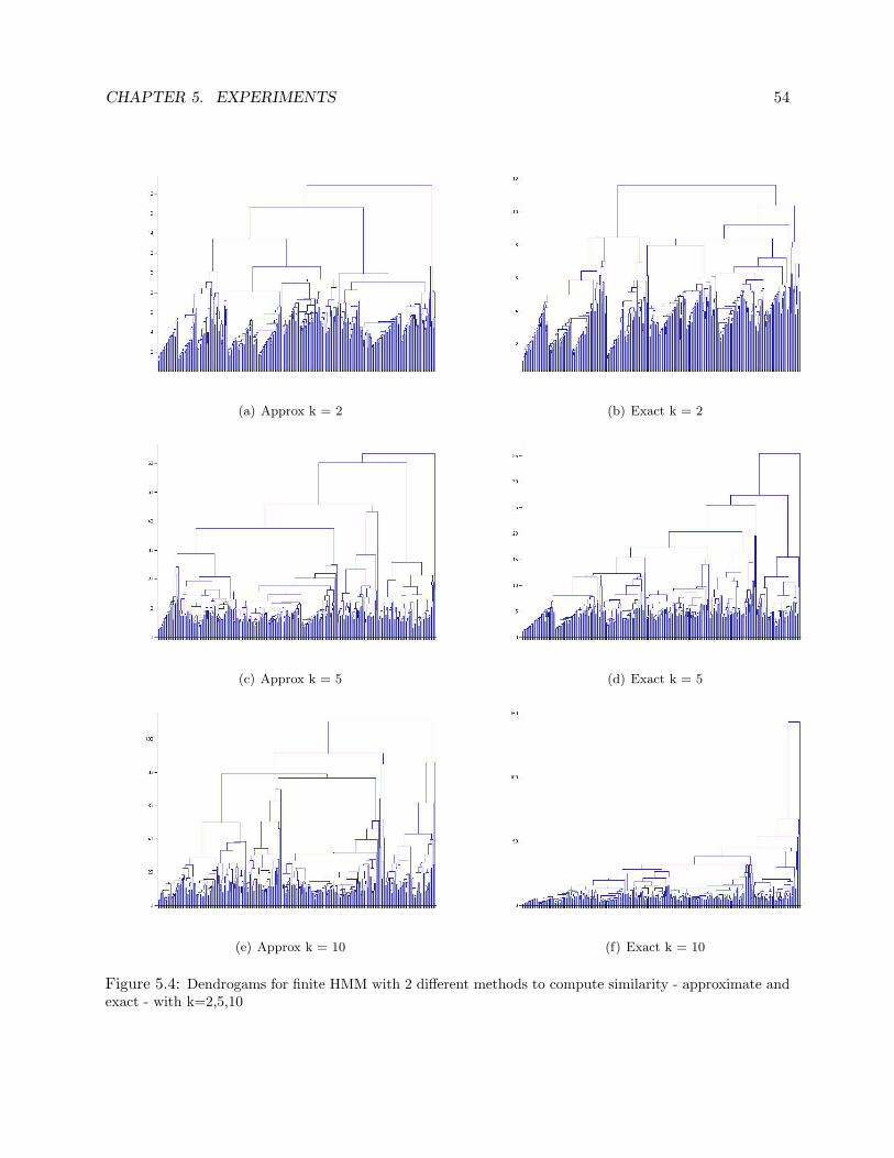
CHAPTER 5. EXPERIMENTS 54
(a) Approx k = 2 (b) Exact k = 2
(c) Approx k = 5 (d) Exact k = 5
(e) Approx k = 10 (f) Exact k = 10
Figure 5.4: Dendrogams for finite HMM with 2 different methods to compute similarity - approximate andexact - with k=2,5,10

CHAPTER 5. EXPERIMENTS 55
with ground truth - which is because the source of labels is correlation analysis (with biology expert
modification).
It is clear from Table 5.2 that most of the winning entries are the HDP-HMM ones - which shows
the clear edge non-parametric methods have over parametric methods. These results shows that
a statistical framework such as HDP-HMM can solve clustering tasks such as the one presented
effectively without overfitting. One of the interesting things about the table is performance of
finite HMM with exact measure of similarity for Cho dataset. The reason behind some of the ‘poor
scores’ is not very clear, but intuition points to sparsity of the data in very large parameter space
or overfitting.
The dendrograms in Figures 5.2 and 5.3 show that most of the agglomeration in the case of
HDP-HMMs happen at a much lower level than most of the finite HMM dendrograms, which
indicates cleaner, well formed clusters in the case of HDP-HMM. Another point worth noting is
that the change across the dendrogram shapes for various settings of hyper-hyperparameters is
small - which again shows that the settings of priors do not influence the learnt model.
The dendrograms for finite HMM, exact metric and approximate metric, in Figure 5.4 are very
similar. This observation combined with the values in Table 5.2 leads us to believe that both
methods give similar probabilistic measures for similarity of two time courses.

Chapter 6
Conclusion
In this thesis we have seen the importance of the problem - namely, clustering gene expression time-
course data. As biologists probe deeper into nature of organisms, a fundamental understanding of
cell, its constituents, and its activities is ever so important. To this end, deciphering the human
genome has been a prime area of research for the last couple of decades and will continue to
remain so for a long period of time to come, and clustering genes is one of key areas of research
in bioinformatics. Machine learning and computational biology are two very useful tools used by
bioinformatics’ researchers in solving problems related to human genome.
Our solution to the above problem involves state of the art Bayesian approach to clustering
- application of HDP-HMM to gene expression time-course clustering. By setting the traditional
hidden Markov model in a hierarchical framework we are able to get around the model selection
issue, and at the same time, by having a Dirichlet process in a hierarchical setting, we have made the
state space of the HMM countably infinite. In short, we are able to address both the shortcomings
of earlier methods like correlation analysis (discarding time aspect of the data) and finite HMMs
(fixing model complexity beforehand).
We believe that we have successfully shown the applicability of HDP-HMM to gene clustering.
However, having said this, we feel that there are still a few issues we need to address and few areas
we need to explore further in order to firmly establish HDP-HMM’s suitability to such tasks.
56
CHAPTER 6. CONCLUSION 57
6.1 Future directions
Some of the areas need further exploration. Prime among those are leave-one-out analysis. It would
be interesting remove a gene from the training set, and learn the model. Once learnt, the predictive
density on the unseen time course can be calculated and this could be an indicator of how well the
data is modeled. Another approach, apart from predictive density, is to classify the unseen data
point as belonging to one of the C clusters.
The other area that we would like to explore is applying the model to different datasets and
synthetic datasets. Synthetic time series datasets can be produced using sine functions with suitable
noise added, with time points chosen at regular intervals, starting at some random point. Another
method to generate synthetic dataset is using spline equations with suitable noise. An advantage
of using synthetic data is availability of huge quantities of labeled data, using which we can the
determine the scalability of models as both, number of time courses as well as number of time points
increase. Another advantage being the ability to tweak the dataset to test the various aspects of
our models like missing data and unequally spaced time points.
It would also be interesting to compare our model to other models and methods. One of
them being CAGED, a publicly available clustering package, exclusively aimed at clustering gene
expression time courses. Another statistical time series model that would make an interesting
comparison would be a Bayesian HMM. HDP-HMM is Bayesian by construction - we integrate
of the Gj ’s at the group level (remember the Chinese restaurant process and Chinese restaurant
franchise metaphors). However, a finite HMM trained using the Baum-Welch algorithm gives the
ML estimates of the parameters (A, C, and π). In order to obtain a Bayesian version of a finite
HMM, we can incorporate a prior over these parameters and integrate over the prior.
Sampling based exact metric for HDP-HMM: At present we do not have a way to compute the
exact metric for the infinite HMM, as we do for the finite HMM (5.3); it is possible however to
compute a stochastic estimate of the probability in (5.3) by sampling many finite instantiations
of the HDP-HMM, each of which have a fixed number of hidden states and associated point pa-
rameters. The measures of dissimilarity for each sampled finite HMM can then be computed and
averaged. This is a computationally expensive solution for the infinite model, but at present is the

CHAPTER 6. CONCLUSION 58
only available algorithm to compute this metric.
Despite the areas for further exploration mentioned above, we consider the study done as a
part of this thesis points to the success of HDP-HMM (and non-parametric Bayesian methods in
general) to complex statistical modeling tasks. Moreover, we have addressed an important issue in
bioinformatics and have provided a novel way to approach problems in bioinformatics.

Bibliography
D. Aldous. Exchangeability and related topics. In Ecole d’ete de probabilites de Saint-Flour XIII–
1983, pages 1–198. Springer, Berlin, 1985.
Z. Bar-Joseph, G. Gerber, D. Gifford, T. Jaakkola, and I. Simon. Continuous representations of
time series gene expression data. Journal of Computational Biology, 10(3–4):241–256, 2003.
L. E. Baum and T. Petrie. Statistical inference for probabilistic functions of finite state Markov
chains. Annals of Mathematical Statistics, 37(6):1554–1563, 1966.
L. E. Baum, T. Petrie, G. Soules, and N. Weiss. A maximization technique occurring in the
statistical analysis of probabilistic functions of Markov chains. The Annals of Mathematical
Statistics, 41:164–171, 1970.
M. J. Beal, Z. Ghahramani, and C. E. Rasmussen. The infinite hidden Markov model. In Advances
in Neural Information Processing Systems 14, Cambridge, MA, 2002. MIT Press.
D. Blackwell and J. B. MacQueen. Ferguson distributions via Polya urn schemes. Annals of
Statistics, 1:353–355, 1973.
D. M. Blei, M. I. Jordan, and A. Y. Ng. Hierarchical Bayesian Models for Applications in Infor-
mation Retrieval. Baysian Statistics, 7:25–44, 2003.
R. J. Cho, M. J. Campbell, E. A. Winzeler, L. Steinmetz, A. Conway, L. Wodicka, T. G. Wolfsberg,
A. E. Gabrielian, D. Landsman, D. J. Lockhart, and R. W. Davis. A genome-wide transcriptional
analysis of the mitotic cell cycle. Molecular Cell, 2(1):65–73, 1998.
59
BIBLIOGRAPHY 60
A. P. Dempster, N. M. Laird, and D. B. Rubin. Maximum likelihood from incomplete data via
the EM algorithm. Journal of the Royal Statistical Society, Series B (Methodological), 39:1–38,
1977.
M. B. Eisen, P. T. Spellman, P. O. Brown, and D. Botstein. Cluster analysis and display of genome-
wide expression patterns. Proceedings of the National Academy of Sciences of the USA, 95(25):
14863–14868, December 1998.
T. S. Ferguson. A Bayesian analysis of some nonparametric problems. Annals of Statistics, 1(2):
209–230, 1973.
L.H. Hartwell and M.B. Kastan. Cell cycle control and cancer. Science, pages 1821–1828, 1994.
V. R. Iyer, M. B. Eisen, D. T. Ross, G. Schuler, T. Moore, J. C. F. Lee, J. M. Trent, L. M. Staudt,
J. Hudson Jr., M. S. Boguski, D. Lashkari, D. Shalon, D. Botstein, and P. O. Brown. The
Transcriptional Program in the Response of Human Fibroblasts to Serum. Science, 283(5398):
83–87, 1999.
B. H. Juang and L. R. Rabiner. Hidden Markov models for speech recognition. Technometrics, 33:
251–272, 1991.
C. M. C. Milligan. A Study of the Comparibility of External Criteria for Hierarchical Cluster
Analysis. Multivariate Behavior Research, 21:441–458, 1986.
R. M. Neal. Markov chain sampling methods for Dirichlet process mixture models. Technical
Report 9815, Department of Statistics, University of Toronto, 1998.
L. R. Rabiner. A tutorial on hidden Markov models and selected applications in speech recognition.
Proceedings of the IEEE, 77, 1989.
M. F. Ramoni, P. Sebastiani, and I.S. Kohane. Cluster analysis of gene expression dynamics. Proc.
National Academy of Sciences of the USA, 99(14):9121–6, 2002.
C. E. Rasmussen. The infinite Gaussian mixture model. In Advances in Neural Information
Processing Systems 12, Cambridge, MA, 2000. MIT Press.

BIBLIOGRAPHY 61
G. Salton and M. J. McGill. An Introduction to Modern Information Retrieval. McGraw-Hill, 1983.
A. Schliep, I. G. Costa, C. Steinhoff, and A. Sch onhuth. Analyzing gene expression time-courses.
IEEE Trans. Comp. Biology and Bioinformatics, 2(3), 2005.
J. Sethuraman. A constructive definition of Dirichlet priors. Statistica Sinica, 4:639–650, 1994.
A. Stolcke and S. Omohundro. Hidden Markov model induction by Bayesian model merging. In
S. J. Hanson, J. D. Cowan, and C. L. Giles, editors, Advances in Neural Information Processing
Systems 5, pages 11–18, San Francisco, CA, 1993. Morgan Kaufmann.
Y. W. Teh, M. I. Jordan, M. J. Beal, and D. M. Blei. Hierarchical Dirichlet Processes. Technical
Report 653, Department of Statistics, University of California, Berkeley, 2004.
Y. W. Teh, M. I. Jordan, M. J. Beal, and D. M. Blei. Hierarchical Dirichlet processes. Journal of
the American Statistical Society, 2006. To appear.
D. L. Wild, C. E. Rasmussen, Z. Ghahramani, J. Cregg, B. J. de la Cruz, C-C. Kan, and K. A. Scan-
lon. A Bayesian approach to modelling uncertainty in gene expression clusters, 2002. Extended
conference abstract in 3rd Int. Conf. on Systems Biology, Stockholm, Sweden.
Appendix A
Dirichlet Process theory
Theorem 1: If G ∼ DP (α, G0) and θ1 ∈ Θ is a sample from G, then
G|θ1 ∼ DP (αG0 + δθ1) (A.1)
where δθ1 is a point mass at θ1
Proof: Consider some natural number k and partition B. From the definition of a Dirichlet
Process, we know that
(G(Θ ∈ B1), G(Θ ∈ B2), . . . , G(Θ ∈ Bk)) ∼ Dir(αG0(B1), αG0(B2), . . . , αG0(Bk))
Also, we know that given a fixed value of k and a fixed partition B, G is distributed as a
Dirichlet distribution and the sample φ1 is an observation from a single trial. Hence, from the
posterior for Dirichlet distribution, we have
(G(Θ ∈ B1), . . . , G(Θ ∈ Bk))|θ1 ∼ Dir(αG0(B1) + δθ1(B1), . . . , αG0(Bk) + δθ1(Bk))
The above will hold for all k and all partitions B that might be chosen. Hence,
G|θ1 ∼ DP (αG0 + δθ1)
62

APPENDIX A. DIRICHLET PROCESS THEORY 63
�
Theorem 2: The marginal probability
P (Θ ∈ Bi) = G0(Bi) (A.2)
Proof:
P (Θ ∈ Bi) =∫GdG P (Θ ∈ Bi|G) P (G)
=∫GdG G(Θ ∈ Bi) P (G)
= E[G(Θ ∈ Bi)]
From Definition 1, since
(G(Θ ∈ B1), G(Θ ∈ B2), . . . , G(Θ ∈ Bk)) ∼ Dir(αG0(B1), αG0(B2), . . . , αG0(Bk))
and from definition of Dirichlet distribution, we can write
P (Θ ∈ Bi) = E[G(Θ ∈ Bi)]
=αG0(Bi)∑kj=1 αG0(Bj)
=αG0(Bi)
α
= G0(Bi)
�
Consider how the above marginal probability of Θ ∈ Bi changes under the posterior of G after
APPENDIX A. DIRICHLET PROCESS THEORY 64
θ1 has been sampled:
P (Θ ∈ Bi|θ1) = E[G(Θ ∈ Bi)|θ1)]
=αG0(Bi) + δθ1(Bi)∑kj=1 αG0(Bj) + δθ1(Bj)
=αG0(Bi) + δθ1(Bi)
α+ 1(A.3)
The above leads to what is known as the ‘clustering effect’. Consider the case when k = 2
and B1 = {θ1} and B2 = {θ : θ 6= θ1}. Since Θ is a continuous random variable, under the prior
DP (αG0) we have
P (Θ = θ1) = G0({θ1})
= 0
Under the posterior DP (αG0 + δθ1) after having sampled θ1 however,
(G(Θ = θ1), G(Θ 6= θ1))|θ1 ∼ Dir(αG0({θ1}) + δθ1({θ1}), αG0({θ : θ 6= θ1}) + δθ1({θ : θ 6= θ1})
∼ Dir(1, α) (A.4)
Therefore, under the posterior DP (αG0 + δθ1) after having sampled θ1, the probability of
sampling the same point has a non-zero probability. Thus,
P (Θ = θ1) =1
α+ 1(A.5)
P (Θ 6= θ1) =α
α+ 1(A.6)
Now, extending to the case where we have n samples of θ = θ1, . . . , θn, we can write the marginal
APPENDIX A. DIRICHLET PROCESS THEORY 65
probability of Θ ∈ Bi under the posterior DP as
P (Θ ∈ Bi|θ1, . . . , θn) = E[G(Θ ∈ Bi)|θ1, . . . , θn)] (A.7)
=αG0(Bi) + δθ1(Bi) + . . .+ δθn(Bi)∑kj=1 αG0(Bj) + δθ1(Bj) + . . .+ δθn(Bj)
=α
α+ nG0(Bi) +
1α+ n
n∑i=1
δθi(Bi) (A.8)
The random probability vector under the posterior DP is
(G(Θ ∈ θ), G(Θ /∈ θ))|θ ∼ Dir(αG0(θ) +n∑j=1
δθj(θ), αG0({θ : θ /∈ θ}) +
n∑j=1
δθj({θ : θ /∈ θ}))
∼ Dir(n∑j=1
δθj(θ), α) (A.9)
Therefore under this posterior, the marginal probabilities (that is, integrating out G) of sampling
one of the already chosen θ for the (n+1)th sample and the probability of choosing a distinct sample
are given by:
P (θn+1 = θi for 1 ≤ i ≤ n|θ1, . . . , θn, α,G0) =1
α+ n
n∑j=1
δθj(θn+1) (A.10)
P (θn+1 6= θi for 1 ≤ i ≤ n|θ1, . . . , θn, α,G0) =α
α+ n(A.11)
Let us define an indicator variable Wn to be 1 if θn is distinct and Wn = 0 otherwise. If
N(Θ) =∑n
i=1Wi, then the expected number of distinct samples is
E[N ] = αn∑i=1
1α+ i− 1
(A.12)
Thus from (A.11) and (A.12) above we see that the probability of observing a distinct sample
goes to 0 as n →∞ and at the same time, the expected number of distinct samples goes to ∞ as
n→∞. This illustrates the clustering effect.
The interpretation of α and G0

APPENDIX A. DIRICHLET PROCESS THEORY 66
From (A.7) and (A.8), we know that
E[G|θ1, . . . , θn] =α
α+ nG0 +
1α+ n
n∑i=1
δθi
We can interpret α to be a ‘control knob’ that controls how closely our draw G follows G0.
Thus, as α grows larger, the contribution from the first term of (A.8) increases while that of the
second decreases, and as α gets smaller, the opposite happens. Thus, G0 can be interpreted as a
prior over Θ.
Definition 2: An infinite set of random variables are said to be infinitely exchangeable if for
every finite subset {x1, . . . , xn} we have,
P (x1, . . . , xn) = P (xπ(1), . . . , xπ(n)) (A.13)
for any permutation π.
Theorem 3 (deFinetti (1973)) : A set of random variables is infinitely exchangeable if and
only if
P (x1, . . . , xn) =∫dP (θ)
n∏i=1
P (xi|θ) (A.14)
for some θ and some measure P (θ).
The graphical model representing exchangeability is shown in Figure A.1.
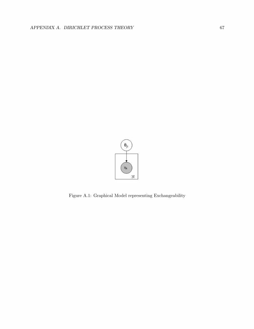
APPENDIX A. DIRICHLET PROCESS THEORY 67
Figure A.1: Graphical Model representing Exchangeability