approved: ga»6„ - vtechworks.lib.vt.edu · through the computer’s screen ... which represents...
TRANSCRIPT
Real Time Generation Station Simulator l
byJaime A. Latorre
Thesis submitted to the Faculty of theVirginia Polytechnic Institute and State University
in partial fulfillment of the requirements for the degree ofMaster of Science
inElectrical Engineering
APPROVED:
ga »6„ ’J e La Ree Lopez, C airman
A.G.Phadke S.Rahman
June 1988i
Blacksburg, Virginia
Eii
Real Time Generation Station Simulator
byJaime A. Latorre
J.De La Ree Lopez, Chairman
Electrical Engineering
(ABSTRACT)
lll,} A real time generation station simulator which is to be used as an operator traineris developed. The software developed simulates a Y-wound generator connectedto an inünite bus through a A/ Y step up transformer and two parallel lines. Theoperation of the generator is simulated under normal or abnormal conditions ofthe power system or the generator itself. The system is simulated in two micro-computers and interaction between the simulator and the operator is providedthrough the computer’s screen and keyboard. Different screen representations
show the behavior of the generator at any moment and based on these the oper-
ator can take any action through the generator controls provided in his keyboard.

I
Acknowledgements
I would like to express my deep gratitude to Dr. J. De La Ree for his constant° encouragement and assistance over the course of this project. I wish to thank
Dr. A.G. Phadke for all the help he also gave me and Dr. S.Rahman for servingon my advisory committee.
Acknowlcdgements iii

M
Table of Contents .
1.0 INTRODUCTION ................................................... 11.1 REAL-TIME SIMULATION ........................................... 11.2 THESIS LAYOUT ................................................... 5
2.0 SYSTEM SIMULATION .............................................. 72.1 SYNCHRONOUS MACHINE MODEL .................................. 82.2 EXCITATION SYSTEM .............................................. 92.3 GOVERNOR AND TURBINE SYSTEMS ............................... 142.4 POWER SYSTEM REPRESENTATION ................................ 16
2.4.1 ONE OPEN PHASE AT THE HIGH VOLTAGE SIDE OF THE TRANSPOR-MER ............................'................................. 18
2.4.2 SINGLE LINE TO GROUND FAULT AT INFINITE BUS ............... 23
3.0 SIMULATOR’S IMPLEMENTATION . . ._............................... 293.1 HARDWARE REQUIREMENTS ...................................... 293.2 SOFTWARE IMPLEMENTATION .................................... 30
3.2.1 KEYBOARD DEFINITION ....................................... 32
Table of Contents iv
M
I
3.2.2 NORMAL GENERATOR’S CONTROL ROOM MIMIC ................. 363.2.3 POWER CAPABILITY CURVE MIMIC ............................. 403.2.4 SYNCHRONIZATION MIMIC ..................................... 42
3.3 EXECUTION PROCEDURE ......................................... 453.3.1 PREPROCESSOR ............................................... 47
3.3.1.1 LINE DIAGRAM DATA ........................... 493.3.1.2 EXCITATION SYSTEM DATA ..................... 51
1
3.3.1.3 GOVERNOR AND TURBINE SYSTEMS DATA ........ 513.3.1.4 GENERATOR CAPABILITY CURVE DATA .......... 52
_ 3.3.2 MA NUAL SYNCHRONIZATION .................................. 533.3.3 AU'TOMATIC SYNCHRONIZATION ............................... 563.3.4 GENERATOR CONNECTED TO THE INFINITE BUS ................. 57
3.3.4.1 CHANGE IN THE SYSTEM CONDITION ............. 583.3.4.2 FINISH SIMULATION ............................ 6I
3.4 EXAMPLE OF A SIMULATION EXECUTION ..............Q............ 62
4.0 RESULTS AND CONCLUSIONS ...................................... 674.1 SIMULATED EVENTS .............................................. 674.2 CONCLUSIONS ................................................... 704.3 FURTHER WORK ................................................. 81
5.0 BIBLIOGRAPHY .................................................. 82
e Vita ................................................................. 84
Table of Contents v

List of Illustrations
Figure 1. One·1ine Diagram .................................. 2Figure 2. Excitation System ................................. 10Figure 3. Exciter Saturation function .......................... 13
Figure 4. Governor and Turbine Systems ....................... 15
Figure 5. Sequence Network ................................. 17Figure 6. One Open-Phase Situation ........................... 20
Figure 7. General One Open Phase Sequence Representation ......... 21
Figure 8 System One Open Phase Sequence Representation ......... 24
Figure 9. System Single Line to Ground Fault Sequence Representation . 25
Figure 10. Reduced Phase to Ground Fault Sequence Representation . . . 26
Figure 11. Operator’s Keyboard deüned Keys ..................... 33
Figure 12. Normal Generator’s Control Room Mimic ............... 37
Figure 13. Power Capability Curve Mimic .......................
41Figure14. Synchronization Mimic ............................. 44
Figure 15. Manual Syncronization in Phase ...................... 71
Figure 16. Syncronization 180 degrees out of Phase 72Figure 17. Permanent Phase to Ground Fault at the Terminals of the gen-
erator ............................................ 73ß
use ofIllustration;vi

I
Figure 18. Phase to Ground Fault at he High Voltage Terminals of thetransformer ....................................... 74
Figure 19. Open Phase at the High Voltage Terminals of the Transformer 75Figure 20. One Transmission Line Removed ...................... 76Figure 21. Loading of Generator with Voltage Regulator in Manual Opera-
tion ............................................. 77
Figure 22. Loss of field ...................................... 78
Figure 23. Abnormal Voltage Regulator Switch from Automatic to Manual 79
List er IllustrationsA
vii

l
NOMENCLATURE
B Mechanical losses coefficient.
6 Generator load angle
D Damping coefiicient. _
E,, Exciter feedback voltage.
Ef, Generator field voltage.
Efdm Exciter output voltage top ceiling,
Efdm Exciter output voltage lower ceiling.W
E, Excitatßin voltage or voltage behind generator impedance.
1~:oME1~1c1.A·ru1uz visa

l
Q Contribution to the fault from the infinite bus.l
I, Current contribution to the fault from the generator.
H Inertia constant.
K, Regulator gain.
K, Exciter tonstant related to self excited field.
K} Regulator stabilizing circuit gain.
Kg GOV€I'I10I' gaifl 600
P, Electrical output power from the generator.
P8, Input power to the turbine.
P„, Mechanical input power to the generator shaft in p.u.
P,,} Power set-point.
S, Saturation function.
T, Regulator amplifier time constant.
T, Governor time constant.
NoMENcLAru1u: · axV _
ITd Open circuit iield transient time constant.
7} Exciter time constant.
7} Regulator stabilizing circuit time constant. A
V, Regulator output voltage.
K,} Regulator reference voltage setting.
V,,d,,, Regulator output voltage top ceiling.
V,m,„ Regulator output voltage lower limit.
V, Generator terminal voltage. a
w Generator speedinw,
System frequencyinXd,
,Xd,, Xd, Sequence reactances for transmission line 1.
X,, ,X,,, Xd, Sequence reactances for transmission line 2.
Xd Direct axis transient reactance. .
Xd, , Xd, Negative and zero sequence reactances of the generator.
NOMENCLATURE . x A

X], ,X]2, X],, Infinite bus equivalent sequence reactances.
Xg„ Generator ground impedance.
AQ, ,X,2, X,,, Equivalent sequence reactances for both transmission lines.
X Series fault impedance created by arc when a phase opens.
X,, ,X,,, X,,, Sequence leakage transformer reactances.
X,„ Transformer ground impedance.
NOMENCLATURE xill„ __.

1n11
A real time simulation of a generation station can be used to predict the behavior
of a generator under fault conditions as well as for operator trainee to react on
time and with the appropriate decision to any system condition.
1.1 REAL- TIME SIMULA TION
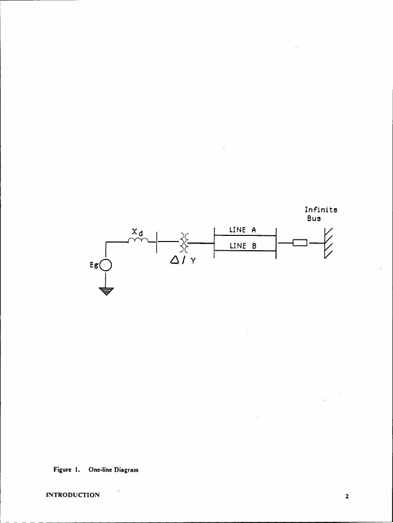
A generator connected to an intinite bus as shown in Figure 1 serves for the
purposes of simulation of the dynamic behavior of a remote generator. The volt-
age at the inünite bus is greatly influenced by large nearby generators in such
awaythat it is independent of events at the remote generator and thus different
fault conditions happening at the generator itself or between the generator and
the infinite bus, which affect the synchronous machine stability can be analyzed.
INTRODUCTION 1
InfiniteBus
Xd LINE Huns6Y
Egg Ö] l
Figure l. One-line Diagram
mrkouucrxow 2

1l
Individually each generator connected to a power system responds to transient
events on the system with variations on the speed-governing systems, tending to
keep each machine at synchronous speed, and with variations on the automatic
voltage regulator trying to maintain a constant voltage at the terminals of the
generator.
In the approach taken the dynamic model of the generator included the classical
transient stability model for the representation of the synchronous machine [1].
The excitation system included the representation of saturation of the generator.
Type I from reference [2] which represents the majority of the excitation systems
now in use, was chosen. The prime mover considered in the simulation was a
non-reheat steam turbine as presented in reference [3]. The automatic voltage
regulator representation is part of the type I excitation system previously men-
tioned.
It is the interest of this work to show the behavior of the generator under any
kind of abnormal conditions on the power system and on the generator itself
which will provide a good understanding of the dynamics of the generator and
will help the generator’s operator to take the right decisions when these circum-
stances occur.
IA diverse kind of abnormal conditions can be simulated at any location of the
power system. An example of these are:
6

1I
l. Three phase faults.
2. Phase to phase faults.
3. Double phase to ground faults.
4. Single phase to ground faults.
5. One, two or three open phases at the high voltage side of transformer
6. Change of load
The system was implemented in two computers, one representing the instructor’s
console and the othe the operator’s console. The instructor from his console can
simulate any of the given conditions. The behavior of the generator is shown onthe operator’s console and a decision based on the readings of the meters can be
made in order to adjust the generator to the new system conditions. A training
session is started by the instructor and is ended at any time by the operator or the
instructor; at the end of the session a summary of activities is created on the op-
erator’s conputer. The instructor inputs all the fault and abnormal conditions I
and the operator takes the appropriate action from his own console to change the
operating conditions of the generator in the same way as he would do it in a
control room. The control’s room meters are simulatedl on his screen and he can
access the generator controls through his own keyboard.
¤N'rRoouc'r1oNl
4
The final objective of this work was to develop a model capable of simulating thereal time behavior of the generator under steady state as well as transient cir-
cumstances, provoked by any of the abnormal power system conditions listed
above or by the generator itself as would be the case of generator start-up and
synchronization to the system. For these situations simple models of the systemelements including the generator were sufficient for the desired purposes.
1.2 THESIS LA YOUT
' Chapter 2 describes the theoretical basis for the simulation. The set of equations
describing the generator dynamics are presented together with the description andsequence representation of the system used. A sequence representation of thesystem is needed to represent the system unbalanced conditions. Two examples
of unbalanced conditions are developed also in this chapter.
Chapter 3 describes how the real·time simulation was implemented to use as an
operator trainer and it presents a detailed manual of the trainer usage and capa-
bilities. A manual synchronization procedure is presented as an example of oneof the trainer’s capabilities to reinforce the understanding of the trainer’s func-tioning.
2
Chapter 4 presents a sequence of simulated events which include unbalanced
faults, in-phase and out of phase synchronization and loss of field. The simulation
INTRODUCTION s
results are shown on plots of different generator parameters, showing the pre-fault, fault and post·fault situations. A list of the parametcrs shown on the resultsare:
• Voltage at the terminals of the generator.F
• Line current.
• Load angle. _
• Frequency.i
• Active power out of the generator.•
• Reactive power out of the generator.
Finally the conclusions are drawn and summarized.
mrnooucrrow 6
l o

”1I1
2.0 SYSTEM SIMULATIONI
In the approach taken to obtain a real time simulation of the generator dynamics
to be used as an operator trainer, the most emphasis was put into the represen- 1
tation of the exciter model, which controls the terminal voltage of the generator.
The synchronous machine representation was chosen with the criterion of pro-
viding a good accuracy during the first swing of the machine (which determines
the stability of the machine) and also the fact that the simulation had to be real-
ized in real time was considered as factor on determining the complexity of the
synchronous machine representation. The governor and turbine systems chosen
provide an approximate representation for fossil-fired plants.
SYSTEM S1MULAT1oN 7
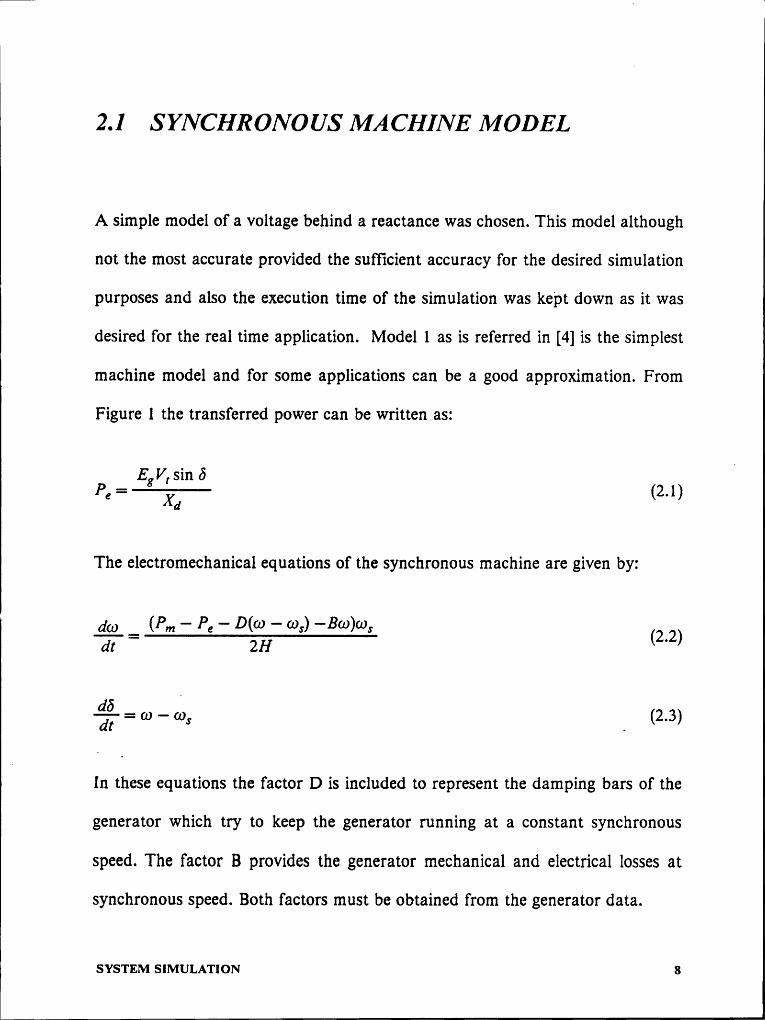
2.1 SYNCHRONOUS MACHINE MODEL
A simple model of a voltage behind a reactance was chosen. This model although
not the most accurate provided the sufficient accuracy for the desired simulation
purposes and also the execution time of the simulation was kept down as it was
desired for the real time application. Model l as is referred in [4] is the simplest
machine model and for some applications can be a good approximation. From
Figure 1 the transferred power can be written as:
P Eg Vs sin 6 2 1H
C -— ° )
The electromechanical equations of the synchronous machine are given by:
Ps — D(w — cos) -Bw)ws (2 2)dz—
2H °
= w — ws s (2.3)
In these equations the factor D is included to represent the damping bars of the
generator which try to keep the generator running at a constant synchronous
speed. The factor B provides the generator mechanical and electrical losses atsynchronous speed. Both factors must be obtained from the generator data.
SYSTEM srmunßmow 6

I I
2.2 EXCITA TION SYSTEM
The excitation system used is shown in Figure 2 which corresponds to type Iexcitation system [2] with the regulator input filter time constant neglected since
is usually very small compared to the other time constants. The saturation func-
tion, whicl· represents a multiplier for E}, to increase excitation when saturation
is reached, is computed from the given excitation values at Efdmx and 0.75E„m„
as it is recommended by IEEE in [2].
The set of differential equations which represent the excitation system is:
dE E - Edr Td
dE,d _ V, — EMS, + K,) (2 5)dt T T2 '
bw, _ T,KP Eb (2 6)dr T Tf °
VIV!dzT2
Along With these equations the regulator and field voltage ceilings have to be
satisfied :
SYSTEM SIMULATION 9

I
I
Se=F(E+'d) .Uref
Umax
Ut + ka Ur 1 Efd 1 E8_ gera Ke + 5*Te 1+ 5*Td >
Eb
5*Kf1 + $*T+°
Figure 2. Excitation System ,_
SYSTEM SIMULATION IO

Efd min S Efd S Ep: max (2-8)
Vr {D10 S V? VF{'DBXThe
upper limit on E}, is set to prevent overheating on the field winding due tothe high field currents. The lower limit on the field voltage is set to prevent over-heating on the rotor poles due to the flux concentration on one end of the polewhen the machine is underexcited. V,,„„, and E},,,„„, need not always to be speci-fied simultaneously.
The output of the regulator is clamped between the minimum and maximum
limits, in order to keep the regulator response within practical limits.
The following expression must be satisfied in steady state condition :
V, - (K, + 5,)Efd = 0 (2.10)
which is also true for maximum values :
Vr max " (Ke + Sel)Efd max = 0 (2*1 1)
Where 5,, is the exciter saturation function defined at Ef,,,,,,,, .
The exciter saturation function is assumed to have an exponential form given by:
5, = K,eK2Ef‘ ‘(2.12)
SYSTEM S1MULAT10N ll

5Where the K, and K, coefficients which determine the exciter saturation curve are 1
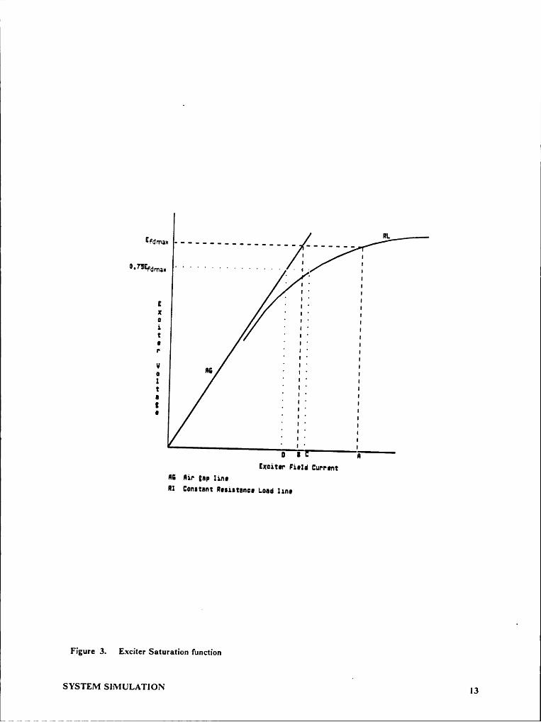
obtained from the two points at which the saturation function is specified. Gen-erally these two points are given for Ef,,,,,„, and 0.75%,,,,,,. From Figure 3 thesaturation function is defined as follows:
x —y5, = -7- (2.13)
Where x and y are points given at the same field voltage and located on the con-stant resistance load saturation and air gap line curves respectively.
In the same way as 5,,, 5,, represents the saturation function at O.75Ef,,„,,,, andthey are defined as follows:
A - B$,,1 = (2- 14)
C - D(2•
1Sincethe exciter saturation function is assumed to have an exponential form thefollowing equations must be satisfied:
(2.16)
(2.17)Solvingthese equations together with equation (2.11) for K, and K2 the followingexpressions are obtained:
1 SYSTEM s1Mu1.A'r1o1~t 12
I
I
II
RLEfdmax ·——·-·——··-——--—- ·---———
I E°·7sEFdrna¤ . ..............I .4°
I Ä I‘ I ‘ IF Ä { I {: · I ' I1 ' I ‘ I‘ I ' IE ‘ I ‘ I·· ~ I ~ 2V gg · I · I° · I · I1 . .·
I · I · I0 · I · II ‘ I · II ' I ' I
T { Y III I R
Exciter Find CUPPIHIIG Ilir gap IinnR1 Constant Ruistancn Load 1in•
Figure 3. Exciter Saturation function
SYSTEM SIMULATION I3

S4K. = % (2.18)
Scl
Sei) SalK =——·———-In —— 2.192 Vrmax ( Sez ) _ ( )
2.3 GO VERNOR AND TURBINE SYSTEMS
The speed governing system together with the turbine are simply modeled to
represent the delays introduced when any action is to take place through them.
A block diagram of this system is shown in Figure 4 from where the dynamic
equations can be written as :
_ dPg„=
P,Cf— Kg(w — cos) — Pg„(220)dr TC
dpm PC,. — P,„
svsmm s1MuLA1·1o1~1 _ I4

«II
+ ..4... ....;... WP Set 1+
1+GovemorSteam Turbine
4 +
oGovernor Gain
Figure 4. Governor and Turbine Systems
SYSTEM SIMULATION 15

2.4 POWER SYSTEM REPRESENTA TION
The genera.tor is connected to an infinite bus, which represents a large (stift)
power system, through a A/Y step up transformer and two parallel lines, asshown in Figure l. The representation neglects the magnetizing reactance of thetransformer and the shunt susceptances of the power lines.
Since any kind of balanced or unbalanced faults are simulated, each element isrepresented using its adequate sequence model. A generalized system represen-
tation using sequence networks is shown in Figure 5. In this representation is as-
sumed that the Y side of the transformer as well as the generator are connected
to ground through impedances X,„ and X,„ respectively. When these impedances
are zero the generator and transformer are solidly ground connected; on the other
hand if these impedances are infinite the generator and transformer will not be
ground connected.
Impedances Xp, Xp, and Xp are equivalent large system impedances and will de-
termine the system stiffness. Looking from the generator side X, , X, and X,
impedances also account for system stiffness; large values of these impedances
will weaken the system contribution to events happening between the generator
and the infinite bus. These element parameters could be varied to test the gener-
ator behavior under different tie conditions. A large impedance on the line will
isvsrmvr SIMULATION 16

I
X alX a X tl X F1X bl ‘' ' ' ‘·""‘* ÜX a2X X t2 X +*2XV
X aoX 0 X X po
X •(fY'Y'Y\„,—l
ax S" ax tn
V
Figure 5. Sequence NetworkSIMULATION ° I7

IIlpermit the simulation of a remote generator or a small impedance will allow the 6
simulation of a close generator.
Three phase faults, phase to phase faults, double phase to ground faults, single
line to ground faults, opening of one, two or three lines at the high voltage side
of the transformer and removal of a transmission line are the events simulatedand for this events in different locations of the power system the generator realtime response is calculated. The contribution of the generator to the system at anymoment for all those situations is to be calculated. As an illustration the genera-
tor contribution to two particular situations is shown.
2.4.1 O1‘lE OPEN PHASE AT THE HIGH VOLTAGE SIDE OF THE
TRANSFORMER
The one open phase situation can be simulated considering that a very high
impedance appear between the terminals of the broken conductor with no corre-sponding impedance on the unbroken phases [7]. Considering an impedance X,appears between the broken phase terminals with X„, X, and X, the impedance
of each of the lines from the generator to the fault location as is shown in Figure
6 the following loop equations can be written:
VM = XJ„,4 (2-22)
SYSTEM SIMULATION 18

1
Vbß = O (2.23)
VCC = O (2.24)
Which can be further written using symmetrical components as:
VM = VM1 + VaA2 + VQA0 = Xr([aAl + IaA2 + [1:,40) (2-25)
VbB=a2VbB1+aVbB2+ VbB0=O (2.26)
VCC = GVCCI + GZVCCZ '(" VCCU =
0Wherethe subindices 1, 2 and O represent the positive, negative and zero se-quence voltages and currents and a represent the complex operator ll20°
Subtracting equation (2.27) from equation (2.26) the following relationship isfound:
VaAl = Va«2 = VaAo (2-28)
And substituting back into equation (2.25) :
VaAl [M2 + [Mo) _(2-29)Which
can be represented as shown in Figure 7.
svsrmm SIMULATION 19l

I
E anI Za I an a >< V F,
'* Varä °E bn Z b I b B
·•· Vba ·E cn ° Z c 1; cg Q C
·•· VcC '
2 n
V
Figure 6. One Open·Phase Situation
I svsram smiumxrxow zoI_ - _

·Zab
X ,. 13
Y va!-I1 ° Y vaÄ2 Y V a°Ä0
Yam Y aA2 Y aao-6-— 4-- ·<——— a3 Z n
Figure 7. General One Open Phase Sequence Representation
SYSTEM SIMULATION 21

1
For the case considered, open phase at the high voltage side of the transformer,a complete sequence representation is presented in Figure 8. From the circuitrepresentation obtained it can be said that there is not any zero sequence comingfrom the generator, which is true since the A/ Y transformer is isolating the zerosequence current from the generator. The system can be further solved for 1,, and-1,,, the positive and negative sequence currents coming out from the generator.Finally it has to be considered that the fault occurred at the high voltage side ofthe transformer which is a A/Y and if the American Standard for designatingterminals H, and X, on Y/A transformers, which requires that the positive se-quence voltage drop from H, to neutral lead the positive sequence voltage dropfrom X, to neutral by 30** regardless of whether the Y or the A winding isuon thehigh tension side, a 90** phase shift when passing positive sequence values fromthe high voltage side to the low voltage side and — 90** when doing the same withnegative sequence values has to be considered [8]. Taking this into considerationthe final sequence voltages and currents at the generator terminals are:
[gl =JI,[gz:
—JI2Vu
= J(Eg ‘ X41]1) (2·33)
V,2 = — J(Xd2I2) (2.34)SYSTEM SIMULATION 22

V,0 = 0 (2.35)
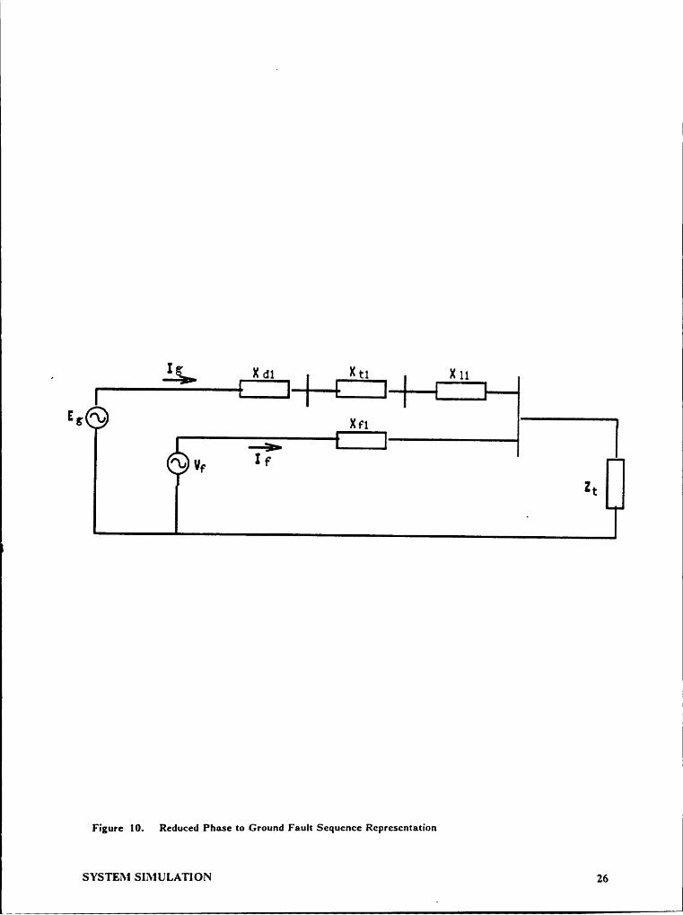
2.4.2 SINGLE LINE TO GROUND FAULT AT INFINITE BUS
It has been demonstrated that for a single line to ground fault at phase a thepositive, negative and zero sequence networks must be connected in series [8] tosatisfy the following fault properties:
Ia[al = [a2 = Ia0 = (236)
Ia Ear:
Whéfß I, 2 and Ü I'Cpl’€S8nl the positive, negative and Z€I'0 SCQUGHCC CUI'I'€nT.S and
impedances. These equations are also satistied on Figure 9. The system can befurther reduced as shown on Figure IO where:
Z, = 3Z,+ ZU + Z2 , _ (2.38)
3X + X + X XZ0 = (239)3X,,, + X,0 +X,0 + Xm
X + X ·+ X XZ2 = (2_4())
SYSTEM SIMULATION 23

X 21
III-IM M—'Ä•
_
V11 hl _ gfI ° Xa2 äXrzV XII, 3:,2I
1 . bz• I 2 1 1V12 '. IQT X30
xdo X1o
-
X*'°1 Xbo
-°-v Vw I ¤1„ V
V
Figure 8. System One Open Phase Scquence Represcntation
svsrma sm1u1.Ar1oN Z4

I
I
I
x dlI
X11 x 11
E6 x+·1IVr
Il d2 x +2 Xx
+*2 YZ +*
. Ia/7 IX10 X 10
I IH tn X
Figure 9. System Single Line to Ground Fault Sequence Reprcsentation
SYSTEM S1>·1ULAT10N ' 25
I
, lg X dl|
X tl X 11
E G X F1Iv,. F
Zt
Figure IO. Reduced Phase to Ground Fault Sequence Rcprescntation
SYSTEM SIMULATION 26

The loop equations can be solved for I, and Q the positive sequence currents fromthe generator and the iniinite bus respectively with the following result:
(Z, + X,,)Eg — Z, V,Ig = (2.41) n
If: (Z, + Xd, + X,, + X,,)Vf— Z,Eg(2.42)A
Where:
A = (Z, + Xd, + X,, + X,,)(Z, + X,,) - Z,Z, (2.43)
And the total fault current is given by:
I = lg + Q (2.44)
Applying current divisors on Figure 9 the negative and zero sequence Currents
from the generator can be calculated as:
X + X + X1, = 1-JL-L-@— (2.45)
3X,,, + X,0 + Xd,
But since the fault occurred at the high voltage side of the transformer and thegenerator is located on the low voltage side of it a phase shift must be made onthe sequence quantities in order to show the corresponding phase shift on the
SYSTEM SIMULATION (27

I
phase quantities between the two sides of the transformer [8]. As in the case ofthe open phase at the high voltage side of the transformer the same phase shiftsoccur for the positive and negative sequence quantities. The zero sequence at theterminals of the generator does not exist. Then the ünal sequence currents andvoltages are given by:
lg] = Jlg . (2.47)
[gz = * JI2
= J(Eg — ]gXd) (2.50)
V,2 = — Ig2Xd2 (2.51)
Vio = 0 (2.52)
SYSTEM SIMULATION · 28

3.0 SIMULATOR’S IMPLEMENTATION
3.1 HARD WARE REQUIREMENTS
The final objective of this real time generator simulator is to use it as a generationstation trainer. The system is implemented in two computers which communicate
each other through the serial port. One of the computers is used by the instructorand the other by the operator.
The main program runs on the operator’s computer and the instructor’s computer
serves as a station from where the simulation is started or finished and the systemconditions are changed. The system was implemented in the following equipment
available at the power systems laboratory:
1. IBM PS/2 Model 50 computer with math co—processor and VGA color mon-itor which served as the operator’s station.
V SIMULATOR’S IMPLEMENTATION 29lt _. MM,-

2. IBM PS/2 Model 30 computer which served as the instructor’s station.
3. Both computers had available the COMI serial port, for communicationpurposes.
_ 4. Serial to serial port connection cable.
The main element of the simulation equipment is the model 50 computer whichprocessor and co·processor run at a l0 Mhz speed. These were a requirement inorder to achieve the real time simulation. The VGA color monitor was a veryuseful tool in the representation of all the system conditions on the operator’sscreen.
If an IBM PS/2 model 50 computer is not available the system can be run on acomparable system with at least the same speed on the processor and co-processor. An EGA color monitor is sufiicient for a good screen representationof the system.
3.2 SOFTWARE IMPLEMENTA TION
The set of algebraic and differential equations which represents the system canbe solved using any of the methods available for the solution of this kind ofproblem. The Runge-Kutta and the trapezoidal methods for solution of differen-
s1MuLAToR·s 1MPL1·:M1;NT.4T1oN 30

tial equations were tried and the trapezoidal method was finally implemented on
the simulat.ion since represented the best choice for a numerically stable solution
[5,6] even if the step size is larger than the smallest time constant together with
the greatly improved execution time very critical in this application.
Given the typical values for the different time constants in the simulated systemand taking into consideration also the smallest duration of a system fault and theaccuracy of the model that didn’t include subtransient reactances in the syn-
chronous machine model, an integration step of 0.02 seconds was chosen in order
to guarantee a real time simulation of the system.
The main program is written in FORTRAN language and the communicationand control routines are written in ASSEMBLER language. Fortran optimizing
compiler was used with all its capabilities in order to minimize the execution time.
Iterative calling of subroutines was avoided as much as possible in the main pro-
gram and when done the number of parameters passed as subroutine argumentswas also minimized; the COMMON statement was preferred to pass variables
from one section of the program to another.
Due to the critical program execution time requirement the main program had to ·
be structured on a way such that real time computation were minimized as muchas possible. An example of this is the big number of pre-computations realized
before the actual simulation starts.
s1MuLAToR·s 1Mr·LEMEm*Ar1oN si

I
3.2.1 KEYBOARD DEFINITION
The control actions normally present in a control room are implemented on the
operator’s keyboard. Figure ll shows the location of the defined keys; its de-
scription and use is as follows:
• INCREASE AND DECREASE INPUT POWER SETTING
These two controls are implemented respectively on the UP AND DOWN
ARROW KEYS The power setting is increased or decreased as long as the
keys are being pressed.
• INCREASE AND DECREASE AUTOMATIC VOLTAGE REGULATOR
SET-POINT
This control is implemented on the RIGHT AND LEFT ARROW KEYS
The automatic voltage regulator set·point is changed as long as the key is
pressed.
•· INCREASE AND DECREASE MANUAL VOLTAGE REGULATOR
SET-POINT
snv1ur.A1·on·s IMPLEMENTATION sze

I
END OF SIMULATION1 DECREASE MANUAL UOLTACE REGULATOR SET•POINT{ { INCREASE MANUAL UOLTACE RECULATOR SET—POINT1 1 1 CHANCE SCREEN MODE1 1 1 1{ { { { UOLTACE RECULATOR 111006I I I : I MAIN CLOSE SWITCH1 1 11 1 1 1 1 1
CHPSI" LOCK111: IE-]—« 1 11 1 11 1 11 11· 1 C 1 ¤1 11 1 1 1 1 1• •FINE ADJUSTMENT KEYS 1 1 1 1 1ENTER CHARACTER DURINC PREPROCESSOR EXECUTION -' I I I Ixucnsnss xnpur powsra ssmnc---------------—---I { { {
DECREASE AUTOMATIC UOLTACE REGULATOR SET-POINT ··-——----···I 1 1IJECREASE INPUT POWER SETTINC·•·•··•·•····•·•·····•·•··':INCREASE AUTOMATIC UOLTACE RECULATOR $ET·POINT ···················
Figure ll. Operator’s Keyboard defined Keys
SlMULATOR’S IMPLEMENTATION 33
I. - -. -- .. ...

l
This control is implemented on the F1 AND F2 KEYS respectively. Themanual voltage regulator set-point is changed as long is the key is pressed.
• CHANGE SCREEN MODE
This control permits the operator to switch the screen from the normal digital”
meter representation to the visualization of the generator capability curve.This function is implemented in F4 KEY and changes screen mode in bothdirections anytime the key is pressed. During the visualization of the genera-tor capability curve the actual load coordinates of the generator are shown
· at every instant.
• MASTER CLOSE SWITCH
This switch is implemented in F10 KEY and its function is to connect thegenerator to the system during the synchronization procedure. As soon asthis key is pressed the generator is connected to the system and the screen ischanged from synchronization to normal operation mode.
• VOLTAGE REGULATOR MODE
This control switch is implemented in F5 KEY and its function is to changethe operation of the regulator from automatic to manual and vice versa. C
| SIMULATOR'S rMr·1.Emm~¤TArxo~ 34

n
• END OF SIMULATION
This software control is implemented in ESC KEY Once this key is pressed
the simulation is ended by the operator and a message is sent back to the in-structor.
• FINE ADJUSTMENT KEYS
Fine adjustment for power input setting, automatic voltage regulator refer-ence and manual voltage setting is provided in the CAPS LOCK KEY . As
the simulation is started gross adjustment is provided automatically by turn-
ing off the CAPS LOCK KEY; at any moment the fine adjustment is desired
for any of the quantities the CAPS LOCK KEY should be turned on. A still
liner adjustment is provided for the automatic voltage regulator reference if
the LEFT SHIFT KEY is pressed at the same time the reference is changed.
j• ENTER CHARACTER DURING PREPROCESSOR EXECUTION
If during preprocessor execution any of the data given is to be changed, then
after selecting the option and entering the new value the SLASH KEYi
should be pressed as the enter key for the value just typed.
srMuLA'roR·s 1M1>r.EMENTA”rroN ss

Z3.2.2 NORNIAL GENERATOR’S CONTROL ROOM MIMIC
A model of this mimic can be seen on Figure 12. The following generator’s metersare simulated during this phase of the simulation:
• GENERATOR TERMINAL VOLTAGE METERS
Indicate the phase voltages in KV of the generator’s terminal bus. Duringnormal balance conditions the value shown is the same- for all three phases,but during unbalanced conditions the values for each phase may greatly differfrom one another.
• SEQUENCE CURRENT METERS
The positive and negative sequence currents are shown. During normal oper-ating conditions or balanced faults the only active meter will be the positivesequence meter but during unbalance conditions the negative sequence cur-
_ rent will reach values that have to be supervised to determine the extent ofdamage that can be done to the machine by its presence during a given periodof time.
F • GENERATOR CURRENT METERS
SlMULATOR'S IMPLEMENTATION 36

I
PHASE A POSITIUE PHASE APHASE B PHASE BNEGATIUEPHASE C PHASE C
VULTAGE IN KV SEQUENCE CURRENTS IN MIPS CURRENT IN MPS.
man xu nm F¤E¤¤EN¤Y IN Nr Luna mm.: m nsunsss
ACTIVE PUIER D4 MI REACTIVE PUIER IN MVAR
FIELU VULTAGE IN VULTS NULL METER 4 VULTAGE REGULATUR
Figure I2. Normal Generator’s Control Room Mimic A
SIMULATOR'S IMPLEMENTATION 37

Z
These meters indicate the current in Amperes in phases A, B, and C of thegenerator.
• GENERATOR SPEED
This meter indicates the speed of the generator in R.P.M.
• GENERATOR FREQUENCY
This meter indicates the generator frequency in cycles per second.
• POWER ANGLE
This meter indicates the power angle of the generator in degrees, which is theangle between the stator magnetic field and the rotor magnetic field. Themeter has a range of 0 to 360 degrees. The slipping pole situation of the gen-erator can be seen in this meter when during this condition the angle increasesfrom its normal operating point value to instability values and back passingthrough the original operating angle. This is a very dangerous situation forthe machine which will work as a generator and motor for consecutive periodsof time gaining speed at all times while the input power is greater than themaximum output power given by Equation 2.1. Under transient instability
ias is the case of a fault or a drastic change of power, the may or may not re-SIMULATOR’S 1MP1.EMENTAT1oN as

lI
store stability depending on the operating condition previous to the event andthe characteristics of the event itself.
• ACTIVE POWER
This meter indicates the generator’s power output, in megawatts. The metercan have negative readings in which case will be indicating a motoring situ-
' ation of the generator.
• REACTIVE POWER
This meter indicates the instantaneous reactive power to or from the genera-tor, When the flow is out of the generator the indication will be positive cor-responding to an overexcited condition; otherwise will be negative and willcorrespond to an under·excited condition.
• FIELD VOLTAGE
This meter indicates the instantaneous generator field voltage which is pro-Vportional to the generator’s field current. (ln steady state If= ä) °J
I• NULL METERs1MuLA1‘oR's 1MPLEM1;NTA1‘1oN 39
·

IThis meter indicates the difference between the manual voltage regulator set-point and the automatic voltage regulator set-point. This meter becomes im-portant when a procedure to take the generator from automatic voltage
regulation to manual voltage regulation or vice versa is to be initiated. InE
both cases a zero indication on this meter by means of varying the adequatevoltage regulator setting, will be a necessary prior step to change the voltageregulator mode to eliminate any possible transient condition which may beundesi. able.
• VOLTAGE REGULATOR STATUS
Gives the actual status of the voltage regulator as Manual or Automatic.
3.2.3 POWER CAPABILITY CURVE MIMIC
Access to this screen mode is possible by pressing the CHANGE OF SCREENMODE KEY when the generator is already synchronized to the system. A rep-resentation of this mimic is shown on Figure 13. On this mode a dot representingthe position of the active and reactive power is presented continuously. Duringnormal operation the dot should stay inside the capability curve limits, but duringtransient conditions big momentarily excursions out of the curve could occur.Different machine design limits could be endangered if the machine is operatedfor a considerable amount of time outside the capability curve limits.
s1MuLA1‘oR·s 1MPLEMENTAT1oN i40

GENERRTDR CRPRBILITY CURVEREFICTIUEPUIERPOUO
FICTIUE PÜIER
Figure 13. Power Capability Curve Mimic
I SlMULATOR’S IMPLEMENTATION 41

3.2.4 SYNCHRONIZATION MIMIC
During synchronization a special control’s room mimic is presented at the opera-tor’s screen showing the necessary meters and apparatus in order to be able torealize a successful synchronization. A model of this mimic is presented in Figure14.
g • GENERATOR STARTING VOLTMETER
Indicates the reduced phase voltages of the generator at the starting bus involts, with 120 volts representing 1 p.u. voltage at the terminals of the gener-ator.
INFINITE BUS RUNNING-VOLTMETER
This meter indicates the reduced phase voltages of the infinite bus. Duringsynchronization the voltage shown in this meter will be the correct voltage forthe unit to be synchronized to the system. The reading is given in volts with120 volts representing 1 p.u. voltage at the synchronizing bus. (The readingfrom 0 to 150 volts result after a PT that reduces the actual terminal voltageto this range.)
• FREQUENCY METER
s1MULAToR's 1MPLEMENTAT1oN 42
l l
Z•Indicates at every moment the generator frequency in hertz. During syn· lchronization this meter must indicate 60 or a slightly larger number indicatingthat the generator frequency is just over the system frequency. At the moment
the synchronization is realized the frequency difference should be around 0.2· hertz.
• PHASE DIFFERENCE METER
Indicates the phase difference between the voltage at the generator startingbus and the system bus. At the moment of synchronization this differencemust be zero or close to zero to avoid synchronization at different voltagepotentials.
• MASTER CLOSE SWITCH STATUSE
Shows the actual status of the main close switch. During synchronizationprocedure this switch remains on the OFF position; when activated the gen-erator is connected to the system instantaneously.
• SYNCHRONIZATION MODE INDICATOR
Indicates whether the synchronization is being realized in manual or auto-matic mode
SIMULATOR’S lMPLEMENTAT1oN 43

PHASE A E PHASE APHASE B PHASE BPHASE C PHASE C
GENERATOR UOLTRGE IN UOLTS IOS VOLTRGE IN UOLTSGEHERATOR FREOUENCY IN H: PHHSE DIFFEREHCE IN DEGREESMASTER SITTCH STATUS ·
•SYNCHRIHIZATIIH MODE
Figure 14. Synchronization Mimic
SlMULATOR’S IMPLEMENTATION 44

• SYNCHRONOSCOPE
A synchronoscope is implemented during synchronization and is activatedwhen the frequency of the generator is between 95 and 105% of the frequencyof the system. The synchronoscope indicates the difference in phase and fre-quency between the generator and the system before the unit is connected tothe system. When the pointer on the synchronoscope is turning clockwise the
generator frequency is larger than the system frequency which means thanthe generator is going too fast. When the pointer on the synchronoscope ismoving counter clockwise the generator is moving too slow. When the pointeris at 12 o’clock the generator voltage and the system voltage are in phase and
when the pointer is at 6 o’clock the generator voltage and the system voltage
are 180 degrees out of phase. ·
3.3 EXECUTION PROCEDURE
Before starting the simulation the serial port communication cable which con-
nects COMI serial ports on both computers have to be installed. _
Introduce the operator’s diskette in drive A of the model 50 computer and then
turn on the machine. Use the DOS diskette to start the instructor’s computer.SIMULATOR'S 1M1>LEMEr~1*rAr1oN 45

1I
To start the instructor’s program introduce the instructor’s diskette in drive A ofC
the model 30 computer and type INST .
To start the operator’s program, with the diskette still in drive A of the model 50computer type OPER.
The first task the programs do is to set up the communication standards betweenboth computers. So any bad connection on the serial port or failure to follow theabove steps will be resembled on any one of the computers on in both if it is thecase. If an incomplete communication procedure is detected by the operator’scomputer the following message will be printed on the screen:
............STARTING COMMUNICATIONS.............
1. CHECK SERIAL CABLE CONNECTIONS
2. TURN ON INSTRUCTOR’S COMPUTER
3. START INSTRUCTOR’S PROGRAM
In the other hand if the incomplete communication procedure is detected by theinstructor’s computer the following message will be printed on the instructor’s
”screen:
SIMULATOR’S ¤Mm.EMsNrAr1or~1 46

............STARTING COMMUNICATIONS.............
1. CHECK SERIAL CABLE CONNECTIONS
2. TURN ON OPERATOR’S COMPUTER
3. START OPERATOR’S PROGRAM
In both cases the instructions have to be followed in the order given in order tobe able to continue the simulation.
3.3.1 PREPROCESSOR
Once the communication is successful a presentation screen appears at the oper-ator’s station and the operator is asked for the data for his simulation.
After a program presentation screen is erased the operator is asked for his name(20 characters maximum). This name will form part of the final record when thesimulation is finished. Next the operator is presented with the following screen:
CHOOSE ANY OF THE FOLLOWING
1. CARDINAL · 3
SlMULATOR’S xMPL1•:MENTA'rx0N 47

2. AMOS l & 2
3. AMOS 3
4. NEW
PRESS 1 ...........4
Options 1 to 3 correspond to implemented systems representing those AEP(American Electric Power) owned generating units [9]. All of them are single·shaftunits. Any one of these generating units can be chosen as a model for the simu-lation and changes are permitted to accommodate it to the particular needs. Inany case the original data files remain unmodified and any change will be storedin the temporary unit called NEW.
If a complete new model wants to be simulated option 4 should be chosen and anew temporary data file will be created and stored for later use. In any case themodifications made are restricted by the model implemented and explained inchapter 2. .
In this case and through all the preprocessor execution any keyboard input dif-ferent than what the answer is expected to be is ignored and the program stays
SIMULATOR’S 1M1·r.EMENTAT1oN 48

e•
at the current position until the right answer is given. After a system is selectedthe following screen is presented:
DO YOU WANT TO SEE THE ACTUAL DATA - (Y/N)
I If "Y" is answered the preprocessor will start showing the default values for theselected case (last system used if option 4 is chosen) and will accept any changesto the default data.
3.3.1.1 LINE DIAGRAM DA TA
While the line diagram data is entered a line diagram of the system is presented l
in the upper part of the screen. All the entered impedances should be in p.u. ofthe generator base.lf the Cardinal unit was selected the following data will appearon the screen:
1. ZDI =· 0.00000 0.20000
2. ZD2 = 0.00000 0.20000
3. ZD0 =- 0.00000 0.14500
I s1Mu1.Aro1z·s 1M1·u:M1·:1~11·A1·1o1~1 49

1
4. ZDN = 0.00000 0.00000
Choose parameter or enter C to continue
All impedances in p.u. of generator base
I ZDI represents the generator’s transient reactance. ZD2 and ZD0 represent theI negative and zero sequence reactances of the generator and ZDN represents the
ground impedance of the generator. The ENTER character during the pre-
processor execution for any system data changed is implemented in the / key .
In case a parameter needs to be changed the new complex value for the
impedance should be entered leaving a space between the real and imaginary
components; again a maximum of 20 characters is accepted. Successively the
transformer, lines and infinite bus impedances are shown and changed in the
same way if desired. Finally some important characteristics of the generator areshown in z: iccessive menus. These characteristics include the rated power (MVA)of the generator, the power factor given by the manufacturer, the terminal voltage
(KV), the field voltage (V), the open-circuit transient time constant, etc... These
characteristics are very important for the determination of the generator capa-
bility curve as well as for the actual simulation.
I srmuparorvs 1M1>r.nMm~z1·A1·1o1~z ” soLi
3.3.1.2 EXCITA TION SYSTEM DA TA
For the next presented menus a visual aid representing the modeled excitation
system is drawn in the upper part of the screen.
As in the line diagram data input the default values are presented and any
change is accepted and updated immediately. In this case the input data will
correspond to the excitation and regulator time and gain constants, together with
the regulator and excitation limits and the data points for the calculation of the
exciter saturation curve.
All the time constants must be given in seconds and the voltages in p.u. of the
field voltage.
3.3.1.3 GO VERNOR AND TURBINE SYSTEMS DA TA
In this case a control loop representing the governor and turbine systems is pre-
sented in the upper half of the screen as the data is presented and /or changed.
As for the excitation system the data in this case corresponds to the governor and
turbine time and gain constants. ‘
SIMULATOR’S 1MPL1·:MENTATxoN . si

Z3.3.1.4 GENERA TOR CAPABILITY CUR VE DA TA
A generator capability curve is drawn with the existing data and a menu is pre-sented to allow for any change on the capability curvenlimits. The variables pre-sented in this case correspond as it is indicated in the capability curve to reactivepower limiting the field current heating, and minimum reactive power limiting thestator core end iron heating,
The values are presented in p.u. of generator MVA base and should be enteredin the same p.u. base.
At this point the preprocessor ends its task and the program will resume here ifthe (Y/N) question had been answered with "N" keeping the initial chosen unitwithout any change. _
The following message is then printed on the operator’s screen:
WAITING FOR THE INSTRUCTOR TO START SIMULATION
The operator then has to wait until the instructor from his station decides on thekind of simulation he wants to initialize on the operator’s computer.
While the preprocessor is being run by the operator the instructor can decide onthe kind of simulation he wants to start on the operator’s computer based on thefollowing menu presented on his screen:
SIMULATOR’S 1MPLEMENTAT10N sz

1
l. GENERATOR AT STEADY STATE AND CONNECTED TO THE INFI-NITE BUS
2. MANUAL SYNCHRONIZATION
3. AUTOMATIC SYNCHRONIZATION
I-Ie can choose the desired option from this menu and subsequent menus will be
presented if required, but all the input data is held by the instructor’s computer
until the operator’s computer is ready to receive it; this is when the execution of
the preprocessor is over.
3.3.2 MANUAL SYNCHRONIZATION
When this option is chosen by the instructor the synchronization screen appears
on the operator’s computer and he can change the generator settings from the
keyboard to fulüll all the prerequisites before synchronization to the system is
realized. i
In general three basic steps must be realized by the operator prior to synchroni-zation:
sxMuLA”roR·s 1Mr·u:Mnm‘AT1oN ss

I
l. The generator voltage (or its transformer) must be equal to the voltage of thesystem to which it is to be connected.
2. The generator frequency must be equal to the system frequency. I
3. The generator voltage must be in phase with the system voltage.
When synchronizing a generator a failure to follow any of these steps could resultin serious electrical and/or mechanical damage to the generator and turbine. Thesimulation allows the synchronization even if the basic steps have not been fol-lowed, so a synchronization out of phase can be simulated.
In order to fulfill the prerequisites the operator has generator controls defined onthe keyboard as described in section 3.2.1. A normal synchronization procedureis described as follows:
1. Bring the machine from zero to near synchronous speed by increasing themechanical input power to the turbine.
2. When the machine is near synchronous speed start increasing the terminalvoltage of the generator. It is not recommended to increase the voltage before
SlMULATOR’S IMPLEMENTATIONI
54

I
the generator has reached a near synchronous speed since the output voltageof the generator is speed dependant.
3. The synchronoscope which is only activated when the generator is within 5%of synchronous speed is the final tool to achieve a successful synchronization.The synchronoscope rotates counterclockwise (slow) when the generator fre-
I quency is lower than the system frequency and rotates clockwise (fast) whenthe generator frequency is higher than the system frequency. The position ofthe synchronoscope gives the angle difference between the voltage at thegenerator terminals and the voltage at the bus where the generator is to be
connected.
At the moment of synchronization is preferred the generator frequency to belarger than the system frequency so the synchronoscope will be rotating in thefast direction at no more than one revolution every six seconds.
If the synchronization is made at I2 o’clock in these conditions, the phasedifference between the generator and the bus voltages will be zero and since
the voltages had been already equated, a complete in phase synchronization
will be realized. In reality the master close switch is closed when the
synchronoscope passes ll o’clock to allow for the delay on the operator’s re-sponse. A synchronization with the syncronoscope steady at I2 o’clock is not
Ädesirable since this could be due to malfunctioning of the synchronoscope.
s1MuLAroR·s 1M1·u;MnN1*A*rxoN ss

I‘I
In a synchronization realized at 6 o’clock the voltages of the generator andthe system bus will be completely out of phase and the voltage difference be-tween both busses will actually be as much as twice of that of the generatoror system bus voltages.
At the moment the synchronization is wanted the operator closes the MAINCLOSE SWITCH and the synchronization screen will disappear and will be re-placed by the normal operation screen, where new conditions can be started bythe instructor.
The operator must now change the voltage regulator from manual to automaticmode since the synchronization is realized with the voltage regulator in manualoperation, to provide a better control over the generator’s terminal voltage. lf theoperator decides to stay with the manual voltage control, at any time the load isincreased the manual voltage reference will also have to be increased. Otherwisean undesired under-excited generator situation may occur where the generatorwill start consuming reactive power from the system.
3.3.3 AUTOMATIC SYNCHRONIZATION
As in manual synchronization the prior steps to synchronization need to be takenby the operator. He has to bring the machine to near synchronous speed and
iequate the generator voltage with the voltage of the bus to which the generator
SIMULATORS 1MPLEMENTAT10N 56
— l
l
is to be connected, but in this case the computer takes over after these conditions
have been met and adjust the necessary controls to realize an in phase synchro-
nization. When the synchronization is finished, as in the manual synchronization
case, the simulation will continue with the normal operation of the generator
connected to the inünite bus and at his point the instructor can introduce anynew system changes.
3.3.4 GENERATOR CONNECTED TO THE INFINITE BUS
E lf option l is chosen by the instructor he is requested with the following input:
ELECTRICAL POWER BEING DELIVERED BY THE GENERATOR TOTHE SYSTEM IN p.u.
And immediately he will be requested with:
GENERATOR TERMINAL VOLTAGE IN p.u.
These data will determine the initial operating point of the generator and at this
point this data is sent to the operator’s screen and the actual simulation is started. ”
As soon as the data is received by the operator’s computer its screen is unfrozen
from the message that was displaying and instead a mimic of the generator’s
SIMULATOR’S 1M1>1.EM1:NrAr1oN 57n _ _ _-

Icontrol room is shown. At the same time the operator’s keyboard is enabled toallow him to take control actions over the generator.
The operator at this moment will see the steady state operating point, set by theinstructor, reflected on his screen. The operator can at any moment change thescreen mode to see the generator operating point situated on the capability curve.He can also change any of the settings of the generator like the input power set-ting, the automatic voltage regulator setting, the manual voltage regulator settingand change the regulator mode from automatic to manual and vice-versa.
The instructor’s screen will present the following menu:
| ENTER ONE OF THE FOLLOWING OPTIONS1. CHANGE IN THE SYSTEM CONDITION t °
2. FINISH SIMULATION
3.3.4.1 (TFIANGE IN THE SYSTEM CONDITION
If Option 1 is selected then the instructor will have the following menu availableto choose a system condition to be simulated: ·
SELECT SYSTEM CONDITION
Ä SlMULATOR’S rmrnsmmrarrou ss

L1
E 11. NORMAL STEADY STATE SYSTEM
2. THREE PHASE FAULT AT GENERATOR TERMINALS
3. THREE PHASE FAULT AT RING BUS _
4. THREE PHASE FAULT AT INFINITE BUS
5. PHASE TO GROUND FAULT AT GENERATOR TERMINALS
6. PHASE TO GROUND FAULT AT RING BUS
7. PHASE TO GROUND FAULT AT INFINITE BUS
8. PHASE TO PHASE FAULT AT GENERATOR TERMINALS
9. PHASE TO PHASE FAULT AT RING BUS
10. PHASE TO PHASE FAULT AT INFINITE BUS ·11. DOUBLE PHASE TO GROUND FAULT AT GENERATOR TERMI-
NALS
12. DOUBLE PHASE TO GROUNDFAULT AT RING BUS
13. DOUBLE PHASE TO GROUND FAULT AT INFINITE BUS
s11v1uLA1·on·s IMPLEMENTATION so
14. OPEN PHASE ON HIGH VOLTAGE SIDE OF TRANSFORMER
15. TWO PHASES OPEN ON HIGH VOLTAGE SIDE OF TRANSFOR-
MER
16. THREE PHASES OPEN ON HIGH VOLTAGE SIDE OFTRANSFOR-MER
17. ONE TRANSMISSION LINE REMOVED
Any of the options presented can be selected by the instructor and he will beasked for the following data afterward:
TIME AT WHICH CONDITION STARTS IN SECONDS
The instructor has here the opportunity to introduce a delay on the starting of the
new condition. This allows him to start conditions at any time without the oper-
ator knowing it.
DURATION OF THE SYSTEM CONDITION IN SECONDS
_ The duration of the new system condition can be on the order of fraction of a
second, seconds or can also be a permanent condition in which case the digits
9999 should be input as duration, by the instructor.
SIMULATOR’S IMPLEMENTATIQN 60

I
I
Consecutive system changes can be input by the instructor. While one condition
is being executed on the operator’s computer, another system change can be inputby the instructor and the execution will be started after the first condition is fin-ished.
3.3.4.2 FINISH SIMULA TION
If this option is selected by the instructor then the simulation at the operator’s
computer is stopped and a summary of the simulation will be ready for evalu-
ation at the operator’s computer.
Through all this simulation the operator sees on his screen the mimics already
described on sections 3.2.2 and 3.2.3 and shown on Figures 12 and 13. The op-
erator can also at any moment change the settings of the generator through the
keys defined on the keyboard and already described on section 3.2.1 and shown
on Figure 11. One of these keyboard defined functions is the ending of the simu-
lation itself in the same way the simulation was ended by the instructor. . _
s1Mu1.A1·o1z·s IMPLEMENTATION 61
I. -- „ , -

l
3.4 EXAMPLE OF A SIMULA TION EXECUTION
The operator and the instructor should follow the starting procedure given at thebeginning of section 3.3. For the completeness of the example a manual synchro-nization is chosen as an example.
The instructor should select this option by introducing option 3 on the first menupresented to him and although a new menu is presented to him any new inputcondition will only be executed after the generator has been synchronized by theoperator. So it is better for him to wait until the generator is synchronized andthe synchronization transients have died to start inputting new conditions to thesystem.
Before starting the synchronization the operator has the choice of going throughthe preprocessor and changing any of the given parameters for a chosen exampleor creating its own by choosing the adequate option. Let’s assume that theCARDINAL UNIT is the one chosen and no parameters are going to bechanged. After taking the appropriate decisions to escape the preprocessor theoperator will be able to start the synchronizing procedure. He will have to exe-cute the following tasks in order to realize a successful synchronization:
1. Start increasing the mechanical input power in order to bring the machine tosynchronous speed. He has to consider that the only power needed to achieve i
snv1uLAroR·s 1Mx>r.EME1~zTArro1~:O
62

this is the turbine and generator mechanical and electrical losses and thisquantity is usually a small percentage of the total rated output power of themachine. Any excess of power will increase the speed beyond the synchronous
speed and will be very difficult to bring the machine back to synchronousspeed. Usually a synchronization procedure takes around 5 minutes. Start
always- with the smallest step (CAPS LOCK ON) when increasing the input
power. The smallest step provides an increment of 0.01 p.u. each time while
the gross step provides an increment of 0.1 p.u.
2. When the machine reaches 95% of rated speed or frequency (57 hertz for a
60 hertz generator) the synchronoscope will be turned on and will start on the
counter-clockwise direction since the generator frequency is smaller than the
system frequency. At this time the operator should also start bringing up theterminal voltage of the generator; this is achieved by incrementing the manual
voltage reference since during the synchronization procedure the automatic
voltage regulator is disconnected. The gross adjustment at the beginning and
the line adjustment at the end should be used to bring the voltage to the de-
sired level which is the same as the voltage indicated by the voltmeters con-
nected to the synchronizing bus on the upper right hand side of the screen.
This voltages should be equated before the machine reaches 60 hertz at whichmoment the synchronoscope starts going clockwise. The voltages shown on
the generator terminals and on the synchronizing bus voltmeters are reduced
voltages, 120 volts corresponding to 1 p.u. voltage at either bus.
srmunmonss uvu>1.1·:1v11z1~1·r„·.1·1o1~z 63

I
3. As the frequency reaches 60 hertz the synchronoscope will slow down to thepoint that at exactly 60 hertz will stop completely at the phase difference in-dicated at that moment and then will start turning clockwise. Thesynchronoscope will start now accelerating in this direction and the operatorshould synchronize, CLOSE THE MAIN SWITCH, when thesynchronoscope is slowly moving and approaching 12 o’clock. A commonpractice is to close the main switch when the synchronoscope is passingthrough 11 o’clock and the turning speed is less then 6 seconds per revolution(frequency below 60.16 hertz).
4. As the generator is synchronized a small transient is created and the genera-tor will stabilize at some operating point where the output active and reactivepower is around zero. This can be seen by the operator in the normal screenmodeor switching to the capability curve mode. Before any attempt is madeto increase this power the generator should be switched from manual voltagecontrol to automatic voltage control. But before doing this the null meter at
the bottom of the screen has to be reading a number close to zero which willmean that the manual voltage setting and the automatic voltage regulatorsetting will produce the same generator terminal voltage. This is achieved byincreasing the automatic regulator voltage setting using the four differentscales provided until the null meter reads the closest number to zero.
A5. After the voltage regulator is in automatic mode, the generator is ready to
start picking up load. Active power is increased by adding the mechanical
s1MuLA1‘oR·s IMPLEMENTATION 64

{11
power to the turbine and reactive power is increased by moving the automaticvoltage regulator setting to the appropriate point. A normal operating pointis located at some point in the first quadrant of the power capability curve,considering that the generator’s normal main purpose is to generate as muchactive power as possible but that should also supply some of the reactivepower needed by the system. Care should be taken when increasing thepower since there is a considerable time delay between the moment the poweris input to the turbines and the actual time the generator’s active power startsincreasing. lt is suggested that this procedure is done slowly, letting the elec-trical power catch up with the input power at given intervals to avoid in-creasing the power beyond the machine limits. The reactive power responseto increments on the regulator setting is really fast since the response takesaction within the excitation system which is a fast system compared to thegovernor-turbine system. In the case of the reactive power the increment step
i of the automatic voltage regulator setting should be well selected since thereactive power is usually very sensitive to changes on the terminal voltage andin general big jumps in the operating point are undesirable.
The generator is now running at synchronous speed completely synchronized tothe system and operating at the operator’s chosen point. The instructor can nowselect to change the system condition by introducing any of the I7 abnormalsystem options presented to him. Let’s assume that the instructor chose faultnumber 6 which is a phase to groumd fault at the high voltage side of the trans-former ; to the next question, time at which condition starts in seconds , he re-
s1MuLA*roR·s IMPLEMENTATION , 66

l
sponded 60 ; and to the question Duration of the system condition in secondshe responded 0.08 This means that 60 seconds after he finished entering thefault duration, an 80 millisecond phase to ground fault will be simulated on theoperator’s computer and after that the fault is cleared and the system returns toits normal steady state configuration.
The operator on the other hand will be at his console waiting for any conditionto be started from the instructor’s console. He will not know when the conditionwill be started due to the delay allowed on the instructor’s console to the startingof the fault condition. With the condition just input, the chances are he will notbe able to identify the kind of fault due to the short duration of the fault; butwith longer conditions he may be able to identify the situation by looking at thevoltage and current phase meters as well as to the sequence meters, the poweroperating point either on the digital meters or in the capability curve. For exam-ple for a three phase fault at the generator terminals he should be able to see thegenerator terminal voltage drop to zero at the same time that the current in-creases equally on all three phases and he should not observe any negative se-quence current. The active and reactive power will drop to zero during theduration of the fault and this can be seen very clearly if the operator switches tocapability •:urve mode.
The operator will continue to see in his screen all the events sent from the in-structor console and in some of those he may need to take control actions. Thesimulation is finished by either the operator or the instructor.
SIMULATOR’S IMPLEMENTATION 66

4.0 RESULTS AND CONCLUSIONS
4.1 SIMULA TED EVENTS
Various tests were made on the CARDINAL unit which data was obtained fromAEP [9]. The unit is connected to the infinite bus through the standard A/Ytransformer and the two parallel lines system implemented in the simulation.
The results presented are part of the variables that are normally displayed onithescreen. The results on the screen are updated 2 times per second while in thegraphs presented a very fine updating time of 0.02 seconds was used.
~ Figure 15 shows the corresponding diagrams for a manual in phase synchroniza-tion. Although an actual 0 degree phase difference is difficult to acomplish man-ually, it can be seen that the transients created due to a phase difference between
the generator terminal voltage and the synchronizing bus voltage of approxi-
Rzsuurs AND CONCLUSIONS 67
6
mately 5 degrees are very small and the machine comes to steady state very rap-idly.
Figure 16 on the other hand shows a synchronization attempt at 180 degrees outof phase. In this case very big excursions in all the plotted variables occured. Iffor example the current variations in both .synchronizations are compared it canbe seen that while during the in phase synchronization the highest value for cur-rent was 0.13 p.u, during out of phase synchronization it reached values close to1.8 p.u. A situation like this is very likely to damage the machine.
Figure 17 shows a permanent phase to ground fault at the generator terminals.A situation very likely to happen since usually the brakers are situated at the highvoltage terminals of the transformer. While the voltage on the faulted line re-mains at 0 volts, the automatic voltage regulator brings up the voltage on theother phases which results on the situation shown on which the machine stillsupplies active and reactive power to the system at a smaller load angle and at avery high and dangerous current through the faulted phase. Since the situationis unbalanced, negative sequence components are also created and the machinecould be easily damaged.
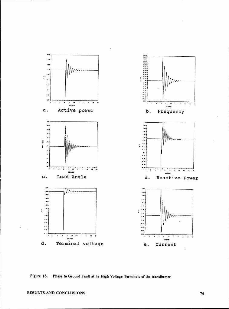
In Figure 18 a phase to ground fault at the high voltage terminals of the trans-former is presented; the fault is assumed to be cleared after 5 cycles. This is acommon fault situation for the system and during the transient created in thiscase the machine stays in synchronism.
Rßsums AND CÖNCLUSIONS 68
L-

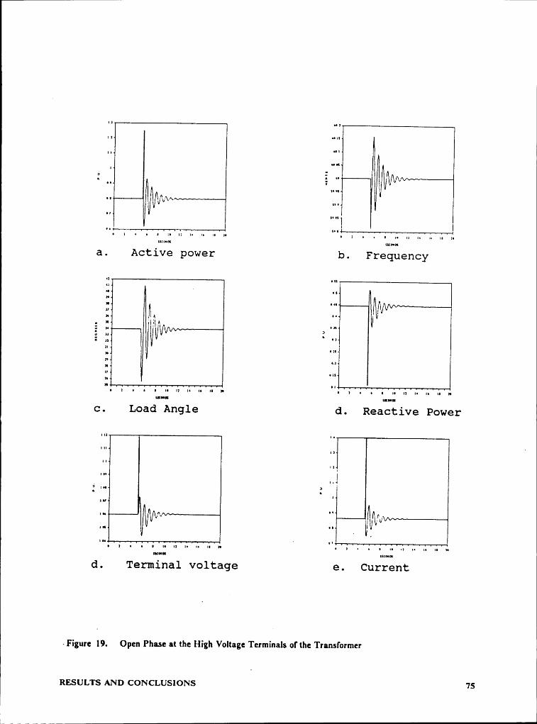
Figure 19 represents a temporary loss of one phase at the high voltage terminalsof the transformer. The transient created in this case is not a critical one and themachine stays in synchronism.
Figure 20 shows a permanent loss of one of the transmission lines of the system.The regulator action brings the voltage to the original level and the governoraction keeps the output power at the level set by the power input reference. Themain characteristic of the new steady state situation is that the machine will beoperating at a higher load angle and so it will be closer to instability if a new faulton the system occurs.
A very common mistake by power plant operators happens during the synchro-nizatiori procedure. When the machine is already synchronized to the system, theoperator must change the voltage regulator from manual to automatic operationbefore he actually starts loading the machine. Figure 2l shows how the machinestarts absorbing reactive power from the system as the machine is loaded whenthe voltage regulator is in manual operation, and the manual voltage reference isnot changed during the procedure.
The loss of field situation is ilustrated in Figure 22. The machine was operatinggiving active and reactive power to the system when suddenly the field is lost. The
machine will not be able to generate any active power since the induced voltageibecomes zero and at the same time will start absorbing reactive power from the
system. The machine rapidly losses synchronism. This situation is never wantedl
Rßsums AND CONCLUSIONST
69

lin a synchronous machine and good protections exist to limit the damage done to
it.
Another similar situation to the machine happens when the voltage regulator ischanged from normal automatic operation to manual operation without the re-quired pre-requisite of nulling the corresponding meter. In the case shown inFigure 23 the machine was operating at a normal operating point and when thevoltage regulator was changed from automatic to manual, the manual voltage
reference was set such that the machine would be underexcited. The machine
rapidly losses synchronism and stays in a slipping pole situation changing oper-ating points continuously.
4.2 CONCLUSIONS
A real time generation-station simulator which represents the behavior of thegenerator under normal or abnormal conditions was developed. The model de-
veloped included an approximate model for the synchronous machine, a verygood model for the excitation system and an approximate model to simulate the
governor action.
With the developed model, the generator respond to slow transients can be
mod-eled.The transients can be either produced by external faults on the system tying E
masums AND coucwsrons 70

I
IJ;
ZIIII · ::;I II :::4II""¤*Ä' „„ I.· ~|l•·•••]v 1•••4'
a. Active power b. Frequency
:II .mIIllIV
1II °°°' II•2IIIIIg"‘-· —
‘ •••¤
c. Load Angle d. Reactive Power
I‘ |••1 ‘
III., .„1 ••1 I_Ä I IIII IId.Terminal voltage e. Current
FFigure I5. Manual Syncronization in Phase
RESULTS AND CONCLUSIONS 71

J
‘ ••1 l J \,_"HI'?SEJJ EEEE J‘1::;. L. J ' JI 2 • • I II I} «• II Il N
N.!1 I • I II Il ll in II II
a. Active power b. Frequency
ui ‘ I!ui ·Il1
Ä Ü¤.„ Äh?_„ y ' 7 . · ...J JV·“ . ZIIJ
c. Load Angle Id. Reactive Power
jfäl
IIInnd.
Terminal voltage e. Current
Figure 16. Syncronization l80 degrees out of Phase
Rzsums AND coxcwsrows 72
J

« I
•• I/V\/\4V\^ N1
‘ n‘
é „ ,V_
a. Active power b. Frequency
'· ZI ,“ •¤ ’/‘· II I . 1:; / I I
ä •• * **1 l
Ii I
III
Ic. Load Angle d. Reactive Power _
d. Terminal voltage e. Current
IIIFigure I7. Permanent Phase to Ground Fault at the Terminals of the generator I
RESULTS AND CONCLUSIONS 73 I
Ii· I
III
SEEEE .:::;; f ___ III?} [• > • • • ·• ·¤ ·· =• =• =• >
a. Active power b. Frequency
. " III Ic. Load Angle d . Reactive Power
I OIIIII gg
,' il I•h1 H: I· - III III} J I.“I
1 0 O I II I} I• I• II II·"_F-vä-_Y——*
d . Terminal voltage e . Current
Figure l8. Phase to Ground Fault at he High Voltage Terminals of the transformer
RESULTS AND CONCLUSIONS 74
III
ä .. ·· IIIII/~II “•{ {
'•a. Active power b. Frequency
= I II: " ,,,6 1: II/VV 2c. Load Angle d. Reactive Power
5 IOC J ä
IO!·'d.
Terminal voltage e. Current
«Figure 19. Open Phase at the High Voltage Terminals of the Transformer
RESULTS AND CONCLUSIONS 75

a. Active power b. Frequency
°|ÄÄ]1MI*1 133 3 ...32*1 11 I ' 3 “ .„i .
c. Load Angle d. Reactive Power
IIII .
IIIIxr:
•u¤.•••°im_ •nd.
Terminal voltage e. Current
Figure 20. One Transmission Line Removed ‘
RESULTS AND CONCLUSIONS 76

l
O —————l——1-0.02-1
-0.04 I-0.06-0.08-0.1
_ -0.12-0.14E -0.16 ·O -0.18-0.2
-0.22 .-0.241-0.26 1‘1-...281 \ E-0-30
0.2 0.4 0.6 0.8P 1n p.u.
0.8
0.7
0.6
0.5
2° 0.4Em
0.3 „
10.2
'0.1I
OI,
I .
0 20 40 60_ DELTA 1n degrees
Figure 21. Loading of Generator with Voltage Regulator in Manual Operation
RESULTS AND CONCLUSIONS 77

0.40.3 10.20.1
0-0.1 1_O•2
-1“ -0.3 - /——·-—ä O. \1:
_' il ?...I6‘°·$ 1 / /./E ;·-,:1-.__$ . ‘ \
‘
1 1 !:· I / '-0.7 ,1.1 11. 1. IO 8 gi 1.;
’,’,·’ J,«
~‘-1.2 , ,-0.7 -0.5 -0.3 -0.1 0.1 0.3 0.5 0.7P in p.u.
0.80.70.6 ä
0.3 /-3I
^.- °·2 0.¤ °·'„_,„-•'¤:O · fg ; gg; $:2·— '•' — —·-·_„°“
-0.1 1‘*"§«··=-‘*‘*-'" ’-0-3 I. 1-0 4 \\‘:-0.6..-0.7 , 1-200 -100 0 100 200
‘DELTA 1n degrees
1
Figure 22. Loss of field
RESULTS AND CONCLUSIONS 78

III
0.5 —————i .—-... -0.40.30.20.1
0-0. 1
_O~2‘
-*.’ . ‘OI3.-
-0.4 ,A ,-<* I0-05 M ¤.?$I<$&\', 0* ..221/,- i' "'"‘-0.6’(
/ //1%/, JI/¤_O7 Q! \Ig’I<m/QTIIII.;/?};j._¤.5 l;—_‘·¥E;§m\, I I° II4II.‘=I¢‘I~.€I‘.l"_'—.¥'-.·‘ ’.·‘*"IIII‘“.I!II·‘I.=' ’ .·
9I \¥°—I“\§-‘ —_ . -. -:**;%:*1 ”T}?.’" .\»~-- X- 1*/T/’
72 X -:__-0.8-0.6 -0.4 -0.2 O 0.2 0.4
I 0.I60.8
P in p.u.
0.90.80.70.6
% 2-A0.4
QÖ: ’ ‘~·I02 *:4..:€.- ‘~.
°* O']='E0 -_-»¤-
-0°°’ I_3 3 ·‘
—<>·I-0.5-0.6 ß-0.7 -/-0.8 7-200 -100 0 100 200
DELTA in degrces
Fi ure 23. Abnormal Volta c Re ulator Switch from Automatic to Manual8 8 8
RESULTS AND CONCLUSIONS 79

IIII
the generator to the iniinite bus or by variations of the settings of the generatoror even internal faults in the generator like a loss of field situation.
The system implemented in two computers representing an instructor and anoperator can simulate a good number of faults from the instructor’s computerand at the same time the operator can vary all the generator settings to move the
generator from one operating point to another, including start-up and synchro-
nization to the system, and thus becomes an excellent tool for training
ofgeneration-station operators.
The power capability curve dynamic screen representation becomes very impor-
tant in the simulation of some if not all operating conditions of the generator. In
particular the excursion of the operating point during a loss of field situation be-
comes very representative of the actual conditions at which the generator is
working.
The meter representing the negative sequence component of the current becomes
also a very useful tool for the operator to make any decision, when this meter
indicates an abnormal reading during a considerable period of time.
RESULTS AND CONCLUSIONS · 80

I
4.3 FUR THER WORK
For the system developed all the interaction between the simulation and the op-erator is through the screens representing the meters and the keyboard repres-enting the controls normally available at a generation station control room. Buta further and more reallistic development would be if the actual generation sta-tion enviroment is included in the simulation.
In order to achieve this the screen representation could be changed by actual an-alog meters implemented in a similar panel like in the generator’s control roomtogether with the necessary switches or controls to change the generator settingsfrom the same panel. The developed simulation can be interacted with this panelby the use of the corresponding D/A, A/D and I/O cards. The digital generatoroutput can also be used to reconstruct a sine wave in order to drive a realsynchronoscope which would form part of the generator’s panel.
With this implementation developed, more functions could be added to the actualsoftware developed. Actually a large number of additional tools could be imple-mented to allow anybody interested to have a clearer idea of the behavior of theIgenerator under different situations.
RESULTS AND CONCLUSIONS 81

III
5.0 BIBLIOGRAPHY
1. C.C. Young, "Equipment and System Modeling for Large-Scale StabilityStudies" ; IEEE Transactions on Power Apparatus and Systems, Vol.PAS-91, No. 1, Jan./Feb. 1972, pp. 99-109.
2. IEEE Committee Report, "Computer Representation of Excitation Sys-tems" ; IEEE Transactions on Power Apparatus and Systems, Vol.PAS-87, No. 6, June 1968, pp. 1460-1464.
3. IEEE Committee Report, “Dynamics Models for Steam and HydroTurbines in Power System Studies" ; IEEE Transactions on Power Ap-paratus and Systems, Vol. PAS-92, No. 6, Nov/Dec. 1973, pp. 1904-1915.
4. P.L. Dandeno, R.L. Hauth, R.P.Schu1z, "Effects of Synchronous Ma-chine Modeling in Large System Studies" ; IEEE Transactions on PowerApparatus and Systems, Vol. PAS-92, No. 2, Mar/Apr. 1973, pp.574-582.
5. I—l.W. Dommel, N. Sato, "Fast Transient Stability So1utions" ; IEEETransactions on Power Apparatus and, Systems, Vol. PAS-91, No. 4,Jul/Aug. 1972, pp. 1643-1650. .
6. M. Ratian, M.J.·1-I. Sterling, M.R. Irving, "Rea1-Time Power SystemSimu1ation" ; IEE Procceedings, Vol. 134, Part C, No. 3, May 1987, pp.206-223.
7. A.E. Guile, W. Peterson, " Electrical Power Systems Vol. 1", PergamonPress, Oxford, England, 1977.
lB1BL1ocRAPHY 82

I
I
8. W.D. Stevenson, " Elements of Power System Analysis", McGraw HillBook Company, New York, N.Y., 1982.9. " Generator Training Simulator", Document No. GE·EE-124, American ‘
Electric Power & Service Corporation, Columbus, Ohio, 1987.
srßniocmumv ° sa