approximate analytical investigation of projectile motion ... · pdf fileapproximate...

Approximate Analytical Investigation of Projectile Motion in a Medium with Quadratic Drag Force

Peter S. Chudinov

Perm State Agricultural Academy, Perm, 614990, Russian Federation

(Received October 1, 2010, accepted December 9, 2010)

Abstract. The classic problem of the motion of a point mass (projectile) thrown at an angle to the horizon is reviewed. The air drag force is taken into account in the form of a quadratic function of velocity with the coefficient of resistance assumed to be constant. Analytical methods for the investigation are mainly used. With the help of simple approximate analytical formulas a full investigation of the problem was carried out. This study includes the determining of eight basic parameters of projectile motion (flight range, time of flight, maximum ascent height and others). The study also includes the construction of the basic functional dependences of the motion, the determination of the optimum angle of throwing, providing the greatest range; constructing of the envelope of a family of trajectories of the projectile and finding the vertical asymptote of projectile motion. The motion of a baseball is presented as examples.

Keywords: projectile motion, quadratic drag force, analytical formulas.

1. Introduction The problem of the motion of a point mass (projectile) thrown at an angle to the horizon has a long

history. The number of works devoted to this task is immense. It is a constituent of many introductory courses of physics. This task arouses interest of authors as before [1 – 3]. With zero air drag force, the analytic solution is well known. The trajectory of the point mass is a parabola. In situations of practical interest, such as throwing a ball, taking into account the impact of the medium the quadratic resistance law is usually used. In that case the problem probably does not have an exact analytic solution and therefore in most scientific publications it is solved numerically [4 – 9]. Analytic approaches to the solution of the problem are not sufficiently advanced. Meanwhile, analytical solutions are very convenient for a straightforward adaptation to applied problems and are especially useful for a qualitative analysis. Comparativly simple approximate analytical formulas to study the motion of the point mass in a medium with a quadratic drag force have been obtained using such an approach [10 – 15]. These formulas make it possible to carry out a complete qualitative and quantitative analysis without using numerical integration of differential equations of point mass motion. This article brings together these works [10 -15] within a unified approach and gives a full investigation of the problem. The proposed analytical solution differs from other solutions by easy formulas, ease of use and high accuracy. In this article the following stages of research are consistently described:

– equations of motion and the construction of the trajectory;– analytical formulas for determining the basic parameters of projectile motion (flight range, time of flight, maximum ascent height and others);– analytical formulas for the basic functional dependences of the problem;– the determination of the optimum angle of throwing, providing the greatest range;– constructing the envelope of a family of trajectories of the projectile; – finding the vertical asymptote of projectile motion.All these characteristics are determined directly from the initial conditions of projectile motion - the

initial velocity and angle of throwing. The proposed formulas make it possible to carry out a complete analytical investigation of the motion of a point mass in a medium with the resistance in the way it is done for the case of no drag. In this article the term “point mass” means the centre of mass of a smooth spherical object of finite radius r and cross-sectional area S = πr2. The conditions of applicability of the quadratic resistance law are deemed to be fulfilled, i.e. Reynolds number Re lies within 1 10 3 < Re < 2 10 5 [2].

Published by World Academic Press, World Academic Union

ISSN 1750-9823 (print)International Journal of Sports Science and Engineering

Vol. 05 (2011) No. 01, pp. 027-042

Peter S. Chudinov: Approximate Analytical Investigation of Projectile Motion in a Medium with Quadratic Drag Force

These values corresponds to the velocity of motion of a point, lying in the range between 0.25 m/s and 53 m/s.

2. Equations of motion and the construction of the trajectorySuppose that the force of gravity affects the point mass together with the force of air resistance R

(Figure 1), which is proportional to the square of the velocity of the point and directed opposite the velocity vector. For the convenience of further calculations, the drag force will be written as R=mgkV 2 . Here m is the mass of the projectile, g is the acceleration due to gravity, k is the proportionality factor. Vector equation of the motion of the point mass has the form

mw = mg + R,where w – acceleration vector of the point mass. Differential equations of the motion, a commonly used in ballistics, are as follows [16]

dVdt

=−g sin −gkV 2,

d dt

=− g cosV ,

dxdt

=V cos , dydt

=V sin (1)

Here V is the velocity of the point mass, θ is the angle between the tangent to the trajectory of the point

mass and the horizontal, x, y are the Cartesian coordinates of the point mass, k=a cd S2 m g

=const is the

proportionality factor, a is the air density, cd is the drag factor for a sphere, and S is the cross-section area of the object (Figure 1). The first two equations of the system (1) represent the projections of the vector equation of motion for the tangent and principal normal to the trajectory, the other two are kinematic relations connecting the projections of the velocity vector point mass on the axis x, y with derivatives of the coordinates.

Fig. 1 : Basic motion parameters.

The well-known solution of Equations (1) consists of an explicit analytical dependence of the velocity on the slope angle of the trajectory and three quadratures

V =V 0cos0

cos1kV 02cos20 f 0− f

, f = sin

cos2ln tan

2

4 (2)

SSci email for contribution: [email protected]

28

International Journal of Sports Science and Engineering, 5 (2011) 1, pp 027-042

t=t0−1g ∫

0

V

cos d , x= x0−1g ∫

0

V 2d , y= y0−1g ∫

0

V 2 tan d (3)

Here V0 and θ0 are the initial values of the velocity and the slope of the trajectory respectively, t0 is the initial value of the time, x0, y0 are the initial values of the coordinates of the point mass ( usually accepted t0=x0= y0=0 ). The derivation of the formulas (2) is shown in the well-known monograph [17].

The integrals on the right-hand sides of (3) cannot be expressed in terms of elementary functions. Hence, to determine the variables t, x and y we must either integrate (1) numerically or evaluate the definite integrals (3).

It turns out [10] that, using a special form of organised integration of quadratures (3) by parts in a fairly small interval [θ0, θ] , the variables t, x and y can be written in the form

t=t02V 0sin0−V sin

g 2 , x= x0V 0

2sin 20−V 2sin 2

2g 1

y= y0V 0

2sin20−V 2 sin2

g 2, =k V 0

2sin0V 2sin (4)

We will obtain the first of the formulae (4). The method of calculating the quadratures is based on the use of the relation between an auxiliary variable u=V cos and the independent variable θ. This relation has the following differential form [16]

duu3 =k d

cos3 (5)

We will consider the first of the quadratures (3) and we write it, using the relation u=V cos , in the form

t=t0−1g∫

0

V

cos d = t0−

1g ∫

0

u

cos2d (6)

We take the integral (6) by parts

t=t0−u tan

g │0

1g ∫

0

tandu=t0−V sin

g │0

1g ∫0

tan du

Using relation (5) we convert the last term

1g∫

0

tan du=kg ∫

0

V 3 tan d =−k∫0

V 2sin dt

Hence

t=t0−V sin

g∣0

−ktV 2sin ∣0

k∫0

t d V 2sin (7)

Suppose the range of integration −0=∆ is fairly small. Then the integral in (7) can be

calaulated as the area of a trapezium with bases t0 , t and height h=V 2sin −V 02sin 0 . We have

k∫0

t d V 2sin≈k t0 t

2 ∫0

d V 2sin=12

k t0t V 2sin−V 02sin0

As a result, formula (7) takes the form

t 12=t0 1

2

V 0sin 0−V sin

g

SSci email for subscription: [email protected] 29

29


(the variable ε is defined by last of relations (4)). Finally

t=t02V 0 sin 0−V sin

g 2We can similarly derive the other two formulas (4).

Hence, in a small interval [θ0, θ] the trajectory of the point mass can be approximated by Eqs (4). These formulas have a local nature. We can calculate the whole trajectory very accurately in steps by calculating V(θ), t(θ), x(θ), y(θ) using Eqs (2), (4) at the right-hand end of the interval [θ0, θ] and taking them as the initial values for the following step

V 0=V θ , t0=t θ , x0=x , y0= y

This cyclical procedure replaces both numerical integration of system (1) and the evaluation of the integrals (3). The smaller the value of k the greater the range [θ0, θ] of applicability of the formulas obtained. When k = 0, i.e. when there is no drag, formulas (4) transform to the well-known accurate formulas of the theory of the parabolic motion pf a point mass and become valid for any values θ0 and θ. Moreover, formulas (4) are accurate in those finite intervals of [θ0, θ] where the variables t, x and y depend linearly on the auxiliary variable z = V 2 sinθ.

As calculations show, the trajectory obtained by integrating system of equations (1) and the trajectory constructed using formulas (2) and (4), are identical. Here, to construct the trajectory it is sufficient to use a step ∆=−0 of the order of 0.1◦.

3. Analytical formulas for determining the main parameters of motion of the point massEquations (4) enable us to obtain simple analytical formulas for the main parameters of motion of the

point mass. In Figure 2 we have drawn a graph of the coordinate y (measured in meters) against the auxiliary dimensionless variable R y=−kV 2sin , where R y is the projection of the normalized drag of

the medium on the y axis. We used the following values V0, θ0 and the coefficient k, the corresponding to the movement of the baseball [6]

V0 = 44.7 m/s , θ0 = 60°, k = 0.000548 s2/m2 , g = 9.81 m/s2.

Fig. 2: The graph of the function y = y(Ry).

The variable R y is similar to the above-mentioned variable z. It can be seen that, both at the ascending stage ( the left part of the graph) and the descending stage (the right part) this graph is close to linear. Hence it follows that the maximum height of ascent of the poin mass H can be obtained approximately using formula (4) for y in the finite interval [θ0, 0], i.e. by taking θ = 0 in this formula.


30


From the relation for the maximum height of ascent H we can derive comparatively simple approximate analytical formulas for the other parameters of motion of the poin mass. The four parameters correspond to the top of the trajectory, four – point of drop. We will give a complete summary of the formulas for the maximum height of ascent of the point mass H, motion time Т, the velocity at the trajectory apex Va , flight range L, the time of ascent ta , the abscissa of the trajectory apex хa , impact angle with respect to the horizontal θ1 and the final velocity V1 :

H =V 0

2sin20

g 2kV 02sin 0

, T=22 Hg

V a=V 0cos 0

1kV 02 sin 0cos20 ln tan

02

4

L=V a T, ta=

T−kHV a2

, xa=LH cot0

1=−arctan[ LHL−xa

2 ] , V 1=V 1 (8)

In formulas (8) V0 and θ0 are the initial values of the velocity and the slope of the trajectory of the point mass, respectively. Formulas (8) enable us to calculate the basic parameters of motion of a point mass directly from the initial data V0 , θ0 , as in the theory of parabolic motion. With zero drag ( k = 0 ), formulas (8) go over into the respective formulas of point mass parabolic motion theory.

As an example of the use of formulas (8) we calculated the motion of a baseball with the folowing initial conditions

V0 = 45 m/s ; θ0 = 40° ; k = 0.000548 s2/m2 , g = 9.81 m/s2.

Table 1.

Parameter Numerical value Analytical value Error (%)

Н, m 30.97 31.43 +1.5

Т, sec 5.00 5.06 +1.2

Va , m/s 23.19 23.19 0.0

L, m 117.8 117.4 -0.3

ta , sec 2.35 2.33 -0.9

хa , m 65.36 66.32 +1.5

θ1 , deg -53.04 -54.73 +3.2

V1 , m/s 27.45 27.99 +2.0The results of calculations are recorded in Table 1. The second column shows the values of parameters

obtained by numerical integration of the motion equations (1) by the fourth-order Runge-Kutta method. The third column contains the values calculated by formulas (8). The deviations from the exact values of parameters are shown in the fourth column of the table.

Figure 3 is an interesting geometric picture for Table 1. If we use motion parameters L, Н, хa to construct the ABC triangle with the height BD = LH , segments AD = xa

2 and CD = L− xa 2 , then in

this triangle 0 C 1 husfor the values L = 117.8 , Н = 30.97 , хa = 65.36 we have: = 40.5°, C = 53°.


31


Fig.3: Motion parameters.

4. Analitical formulas for basic functional relationships of the problemFormulas (8) make it possible to obtain simple approximate analitical expressions for the basic

functional relationships of the problem y(x), y(t), y(θ), x(t), x(θ), t(θ).We construct the first of these dependencies. In the absence of a drag force, the trajectory of a point mass

is a parabola, whose equation using parameters H , L , xa can be written as

y(x)=Hxa

2 x (L – x) (9)

When the point mass is under a drag force, the trajectory becomes asymmetrycal. The top of the trajectory is shifted toward the point of incidence. In addition, a vertical asymptote appears near the trajectory. Taking these circumstances into account, we shall construct the function y(x) as

y x =Hx L−x

xa2ax ,

where a – is a negative coefficient to be determined. We define it by the condition y xa =H . We get a=L−2 xa . Then the sought dependence y(x) has the form

y x =Hx L−x

xa2L−2 xa x

(10) Constructed dependence y(x) provides shift of the apex of the trajectory to the right and has a vertical

asymptote, since the coefficient a0 . In the case of no drag L=2 xa , relationship (10) goes over into (9).

Exactly the same way, we construct the function y(t) described as

y t= Ht T −t ta2T−2 ta t

(11)Since T−2 ta0 , the maximum of the function y(t) drifts to the left, to the launching side. From the equations of motion (1) there follows the equation dy/dx = tan θ. From this equation, upon differentiation of Eq. (10) and putting the results in it, we get the expression for x(θ)

x =a311−a1

1a2 tan (12)

Here a1=L/ xa , a2=L−2 xa /H , a3=xa 2−a1−1 .

Putting (12) to (10), we get the function y(θ)


xa2

LH

0 1

A

B

CD

L− xa 2

32

32


y =b1b2−2a2 tan

1a2 tan , (13)

where b1=H a1−12−a1−2 , b2=2H /b1 .

Using (10) and (11), we get the x(t) function

x t =Lw1

2w2w1w12cw2

2 w12a1w2

, (14)

where w1t =t−ta , w2t =2t T −t /a1 , c=2a1−1/a1 .

Using (11) and (13), we construct the function t = t(θ) described as

t =T2

d 1 y ∓H− y d 2−d 12 y , (15)

where d 1=1H

ta−T2

, d 2=T 2

4 H. The minus sign in front of the radical in (15) is taken on the interval

0 ≤ θ ≤ θ0 and the plus sign is taken on the interval θ1 ≤ θ ≤ 0. Another form of the function t(θ) can be obtained from the equation of the motion dy / dt=V sin

likewise formula (12)

t =l21 1−l1

1l3V sin , (16)

where l1=T / ta , l2=ta 2−l1−1 , l3=T−2 ta/ H . The function V(θ) in (16) is defined by

relation (2).

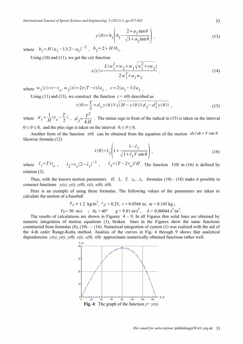
Thus, with the known motion parameters H, L, T, xa , ta formulas (10) - (16) make it possible to consruct functions y(x), y(t), y(θ), x(t), x(θ), t(θ).

Here is an example of using these formulas. The following values of the parameters are taken to calculate the motion of a baseball

a = 1.2 kg/m3, cd = 0.25, r = 0.0366 m, m = 0.145 kg ,V0 = 50 m/s ; θ0 = 40° g = 9.81 m/s2 , k = 0.00044 s2/m2.

The results of calculations are shown in Figures 4 – 9. In all Figures thin solid lines are obtained by numeric integration of motion equations (1), broken lines in the Figures show the same functions constructed from formulas (8), (10) — (16). Numerical integration of system (1) was realized with the aid of the 4-th order Runge-Kutta method. Analisis of the curves in Fig. 4 through 9 shows that analytical dependencies y(x), y(t), y(θ), x(t), x(θ), t(θ) approximate numerically obtained functions rather well.

Fig. 4: The graph of the function y= y(x).


33


Fig.5: The graph of the function y=y(t).

Fig. 6: The graph of the function y=y(θ).

Fig. 7: The graph of the function x= x(t).

Fig. 8: The graph of the function x= x(θ).


34


Fig. 9: The graph of the function t= t(θ).

5. The determination of the optimum angle of throwing, providing the maximum rangeThe formula for the range of throw of the point mass is written as L 0 =V a 0T 0 and is defined

by relations (8). The optimal angle of throwing α , which provides the maximum distance of flight, is a root of equation

dL0

d 0=0

Differentiating the L 0 function with respect to θ0 , after certain transformations, we obtain the equation for finding the angle α when the points of throwing and downs are on the same horizontal

tan2 p sin 44 p sin

= 1 p

1 psin cos2 (17)

Here p=kV02 , =ln tan

2

4 . When k = 0 , equation (17) gives the known solution

α = 45°. When k ≠ 0, equation (17) is easily solved graphically or numerically. The value of the optimum angle α depends on the value of the parameter р. This parameter represents the force of air resistance at the start of motion, referred to the weihgt of the object.

With a condition p=kV 02=const it is possible to change values k and V0 simultaneously. The

optimal angle of throwing α will be alike. But main parameters of motion H , L , T will change as it follows from the formulas (8).

Let the values of motion parameters H1 , L1 , T1 correspond to drag coefficient k1 , and values H2 , L2 , T2 to drag coefficient k2 = qk1 . Then with the condition

p=k1V 012 =k 2V 02

2 =const (18)we get the correlations

H 2=H1q

, L2=L1q

, T 2=T 1

q. The trajectories of the point mass will be similar when the condition (18)

are fulfilled.The graph of function α = α(p) is submitted in Figure 10. The solid line in the Figure is based on the

results of solving equation (17). The dots denote the values of the optimum angle of the throwing obtained by numerical integration (1). The Figure shows that at a sufficiently large interval of the parameter р the solution (17) well approximates the numerical solution.


35


Fig.10: The graph of the function α = α(p).

6. Constructing the envelope of a family of trajectories of the projectileIn the case of no air drag the trajectory of a point mass is a parabola. For the different angles of throwing

under one and same initial velocity projectile trajectories form a family of parabolas. Maximum range and maximum height for limiting parabolas are given by formulas

Lmax=V 0

2

g, H max=

V 02

2g (19)

The envelope of this family is also a parabola, equation of which is usually written as

y x =V 0

2

2g− g

2V 02 x2

(20)

Using (19), we will convert the equation (20) as

y x =H max Lmax

2 − x2

Lmax2 (21)

We will set up an analytical formula similar to (21) for the envelope of the point mass trajectories taking into account the air drag force. Taking into account the formula (21), we will construct an equation of the envelope as

y x =H max Lmax

2 − x2

Lmax2 −ax2 (22)

Such structure of equation (22) takes into account the fact that the envelope has a maximum under х = 0. Besides, function (22) under a0 has a vertical asymptote, as well as any point mass trajectory accounting resistance of air. In formula (22) H max is the maximum height, reached by the point mass when throwing

with initial conditions V0 , θ0 = 90° ; Lmax - the maximum range, reached when throwing a point mass with the initial velocity V0 under some optimum angle 0= . In the parabolic theory an angle α = 45° under any initial velocity V0 . Taking into account the resistance of air, an optimum angle of throwing α is less than 45°and depends on the value of parameter p=kV0

2 . Parameter H max with the preceding

notation is defined by formula [16]

H max=1

2 gkln 1kV 0

2 (23)

A choice of a positive factor a in the formula (22) is sufficiently free. However it must satisfy the condition a = 0 in the absence of resistance ( k = 0 ). We shall find this coefficient under the following considerations.


36


It was shown above, that while taking into account air resistance, the trajectory of a point mass is well approximated by the function

y x =Hx L−x

xa2L−2 xa x , (24)

here x, y are the Cartesian coordinates of the point mass; parameters Н, L, xa are shown in Figure 1. Thus, for the generation of the equation of the maximum range trajectory three parameters are required : H, Lmax, xa . We will calculate these parameters as follows. Under a given value of quantity p=kV0

2 we will find the root α of equation (17). An angle α ensures the maximum range of the

flight. By integrating numerically system (1) with the initial conditions V0 , α , we obtain the values H(α), Lmax = L(α), xa(α) for the maximum range trajectory. The parameter a in the formula (22) we find as follows. We set the equal slopes of the tangents to envelope (22) and to the maximum range trajectory

y x =H x Lmax−x

xa2 Lmax−2 xa x

in the spot of incidence x=Lmax . It follows that parameter a is defined by formulas

a=1−2 H maxH 1−

xa

Lmax 2

(25)

In the absence of air resistance parameter a = 0 .The equation of the envelope can be used for the determination of the maximum range if the spot of

falling lies above or below the spot of throwing. Let the spot of falling be on a horizontal straight line defined by the equation y= y1=const . We will substitute a value y1 in the equation (22) and solve it for х. We obtain the formula

xmax=Lmax H max− y1H max−ay1

(26)

The correlation (26) allows us to find a maximum range under the given height of the spot of falling.

As an example we will consider the moving of a baseball with the resistance factor k = 0.000548 s2/m2

[6]. Other parameters of motion are given by values

g = 9.81 m/s2 V0 = 50 m/s, y1 = ±20, ±40, ±60 m. Substituting values k and V0 in the formula (23), we get H max = 80.26 m. Hereinafter we solve an

equation (17) at the value of non-dimensional parameter p=kV 02 = 1.37. The root of this equation gives

the value of an optimum angle of throwing. This angle ensures the maximum range: α = 40°. By integrating the system of equations (1) with the initial conditions

V0 = 50, θ0 = 40°, x0 = 0, y0 = 0 , we find meanings

H(α)= 36.2 m, Lmax = L(α) = 133.6 m, xa(α) = 75.1 mAccording to the formula (25) the factor is a = 0.149. The graph of the envelope (22) is plotted in

Figure 11 together with the family of trajectories. We note that family of trajectories is received by means of numerical integrating of the equations of motion of a point mass (1). A standard fourth-order Runge-Kutta method was used.


37


Fig.11: The family of projectile trajectories and the envelope of this family.

The results of calculations using the formula (26) are presented in Table 2. The second column of the table contains range values calculated analytically by the formula (26). The third column of the table contains range values from integration of the equations of motion (1). The fourth column presents an error of the calculation of the range in the percentage. Error does not exceed 0.4 %. Formula (26) gives almost the exact value of the maximum range in a wide range of height point drop ( 120 m ). The tabulated data show that formulas (8), (17), (22), (26) ensure sufficiently pinpoint accuracy of the calculation of parameters of motion.

Note that values of H(α), Lmax = L(α), xa(α) can be obtained by using the formulas (8), without numerical integration of the system (1). Substituting V0 and α in the formulas (8), we have

H(α) = 36.5 m, Lmax = L(α)= 132.4 m, xa(α) = 76.0 mFor these values a = 0.2. The graph of the envelope does not nearly change. The right end of the graph

shift along the x axis is less than 1%.

Table 2. Maximum range under different heights of the spot of the falling

y1 , m

Analytical value xmax , m

Numerical value xmax , m

Error ( % )

60 71.2 71.1 0.1

40 98.3 98.3 0.

20 118.0 118.0 0.

0 133.6 133.6 0.

-20 146.6 146.5 0.1

-40 157.8 157.5 0.2

-60 167.5 166.9 0.4

7. Finding the vertical asymptote of projectile motionIt is well known that the projectile trajectory has a vertical asymptote in the resistant medium. We will

deduce an appropximate analytical formula for the value of the asymptote xas = x* (Figure 1). Note that different assumtion formulas can be taken to yield the formula for x*. Accordingly, the final formula for x*

will be also different. This matter is well worth another look. In this paper we are using the first of formulas (1) to solve the task :

dVdt

=−g sin −gkV 2


38


Multiplying the two parts of the formula by the expression dtV

cos , we get the equation

cos dVV

=−g sin cos dtV

−gkVcos dt (27)

From the second and third equations of (1) it follows that

dt=− V d gcos , dx=Vcos dt (28)

Using the ratio (28), we transform the equation (27) to the form

cos dVV

=sin d −gk dx (29)

In turn, the ratio (29) can be written asgk dx=−d cos−cos d ln V (30)

Flight range L is determined by the appropriate formula (8). There is no need to integrate the equation (30) along the whole trajectory. We will integrate the equation (30) only in the interval from x = L to x = xas = x* (Figure 1). We take into account that the value x = L corresponds to the value of the trajectory angle θ = θ1 . The value θ1 is also calcalated with the aid of the formulas (8). We have

gk ∫L

xas

dx=−∫1

−2

d cos− ∫1

−2

cos d ln V (31)

After the substitution of limits in the first two integrals we get

gk xas−L=cos1− ∫1

−2

cos d ln V (32)

To calculate the integral in equation (32) we apply a trapezoidal rule. We split the interval of

integration [ θ1 ,-2 ] in two equal segments with a point 2=

121−

2

. At each of the segments [ θ1,

θ2 ] and [ θ2 ,−

2 ] we calculate the integral in the equation (32) as an area of appropriate trapezoid. We

have

gk xas−L=cos1−12cos1cos 2ln V 2− ln V 1−

12cos2cos −

2ln 1

k− ln V 2

Here symbols V 1=V 1 , V 2=V 2 are introduced . The values V1 , V2 are calculated by

formula (2). We take into account that when θ = ‒2 the point mass velocity accepts the terminal value

Vterm : V −2

=V term= 1k . After some transformations we get the final formula

x* = xas = L + 1

2 gkln [e2 V 1

V 2cos1

k V 1 cos2] (33)

Here е = 2. 71828. Note that using formulas (2) , (8), (33) the value of x* is directly determined by the initial conditions of throwing V0 , θ0 .

As an example, we consider the motion of the baseball for the following parameters [6]:

k = 0.000548 s2/m2, g = 9.81 m/s2 . (34)The calculations are carried out in the following ranges of changes of launch angle and initial velocity :

0 ≤ θ0 ≤ 90°, 20 ≤ V0 ≤ 50 m/s. The results of calculations are recorded in Table 3 and shown in Fig.12 and 13.


39


Table 3. Numerical and analytical values of asymptote x* for different values V0 , θ0

θ0 ,degree 0° 15° 30° 45° 60° 75°

20

30 V0 , m/s 40

50

120.4 122.8

121.5 124.6

114.5117.3

98.8100.9

73.875.3

40.240.9

166.4 165.8

169.1 170.8

160.9 162.7

140.4 141.7

106.7107.5

59.159.7

205.0 200.8

208.8 209.3

200.0 199.9

175.4 175.0

134.5134.3

75.175.5

237.8 230.3

242.7 241.7

232.4 230.3

204.8 202.0

157.6155.8

89.0 88.4

Upper value of each table cell represents the value of x* (in metres) obtained numerically. Lower value of each cell is calculated by formula (33). The numerical values are found by integrating the system of equations (1) with the fourth-order Runge-Kutta method. The table data show that the formulas (2), (8), (33) ensure an accuracy high enough for calcucating asymptote. In Fig. 12 the graphs of dependencies x* = x*(θ0) are plotted for three different values of initial velocity V0 with parameters (34).

Fig. 12: The graph of the function x* = x*(θ0).

The upper curve is for the value V0 = 50 m/s ; the average one– for the V0 = 40 m/s; the lower one – for the value V0 = 30 m/s. The solid line is calculated using the formula (33), the dotted line is plotted on the results of numerical integration of the system (1). It is seen from the graphs that in the considered range of parameters V0 , θ0 formula (33) approximates the function x*(θ0) rather well not only qualitativly but also quantitatively. The maximum value of asymptote is achieved at the significance θ0 ≈ 15° . The analytical formula (33) makes it easy to plot not only the curves x*(θ0) , x*(V0) , but also the surface x*(θ0, V0).

In Fig. 13 the surface x* = x*(θ0, V0) is constructed in the range of arguments mentioned above.


40


Fig. 13: The x* = x*(θ0, V0) surface.

8. ConclusionThe proposed approach based on the use of analytical formulas make it possible to simplify significantly

a qualitative analysis of the motion of a point mass with air drag taken into account. All basic parameters are described by simple analytic formulas. Moreover, numerical values of the sought variables are determined with acceptable accuracy. Thus, proposed formulas make it possible to carry out a complete analytical investigation of the motion of a point mass in a medium with drag in the way it is done for the case of no drag.

9. References[1] D. A. Morales. Exact expressions fot the range and the optimal angle of a projectile with linear drag. Canadian

Journal of Physics. 2005, 83: 67-83.[2] A. Vial. Horisontal distance travelled by a mobile experiencing a quadratic drag force: normalised distance and

parametrization. European Journal of Physics. 2007, 28: 657-663.[3] K. Yabushita, M. Yamashita and K.Tsuboi. An analytic solution of projectile motion with the quadratic resistance

law using the homotopy analysis method. Journal of Physics A: Mathematical and Theoretical. 2007, 40: 8403-8416.

[4] G. W. Parker. Projectile motion with air resistance quadratic in the speed. American Journal of Physics. 1997, 45(7): 606- 610.

[5] H. Erlichson. Maximum projectile range with drag and lift, with particular application to golf. American Journal of Physics. 1983, 51: 357-362.

[6] A. Tan, C.H. Frick and O.Castillo. The fly ball trajectory: an older approach revisited. American Journal of Physics. 1987, 55(1): 37-40.

[7] C.W. Groetsch. On the optimal angle of projection in general media. American Journal of Physics. 1997, 65: 797-799.

[8] J. Lindemuth. The effect of air resistance on falling balls. American Journal of Physics. 1971, 39: 757-759. [9] R.H. Price and J.D. Romano. Aim high and go far – optimal projectile launch angles greater than 45°. American

Journal of Physics. 1998, 66: 109-113.[10] P.S. Chudinov. The motion of a point mass in a medium with a square law of drag.Journal of Applied Mathematics

and Mechanics. 2001, 65(3): 421-426.[11] P.S. Chudinov. The motion of a heavy particle in a medium with quadratic drag force. International Journal of

Nonlinear Sciences and Numerical Simulation. 2002,3: 121-129.[12] P.S. Chudinov. An optimal angle of launching a point mass in a medium with quadratic drag force. Indian Journal

of Physics. 2003, B 77: 465-468.[13] P.S. Chudinov. Analytical investigation of point mass motion in midair. European Journal of Physics. 2004, 25:

73 -79.


41


[14] P.S. Chudinov. Approximate formula for the vertical asymptote of projectile motion in midair. International Journal of Mathematical Education in Science and Technology. 2010, 41: 92-98.

[15] P.S. Chudinov. 2009 Numerical-analytical algorithm for constructing the envelope of the projectile trajectories in midair. http://arxiv.org/abs/0902.0520v1.

[16] B.N. Okunev. Ballistics. Voyenizdat, Мoscow, 1943.[17] S. Timoshenko and D.H. Young. Advanced Dynamics. New York: McGrow-Hill Book Company, 1948.


42

approximate analytical investigation of projectile motion ... · pdf fileapproximate...

Documents