Approximate Computing and

Approximate Circuits (tutorial)

Lukáš Sekanina and Zdeněk Vašíček

sekanina@fit.vutbr.cz; vasicek@fit.vutbr.cz

NASA/ESA AHS 2018, Edinburgh

Tutorial Outline

• Part I: Approximate computing with approximate circuits (Lukáš Sekanina)

• Motivation for approximate computing • Basic principles and techniques • Ad hoc circuit approximation • Automated circuit approximation • Evolutionary circuit approximation • Case studies

• Part II: Formal error analysis methods for approximate computing (Zdeněk Vašíček)

• Error metrics • BDD-based error analysis • SAT-based error analysis • Case studies

• We do not cover • approximate memory, cross-layer approximations, bottom-up

approximations, approximations in SW …

2

Tutorial

Part I: Approximate computing with approximate circuits

3

Approximations have always been with us

• Computer engineering • FP numbers, computer arithmetic, … • S. H. Nawab et al.: Approximate Signal Processing, Journal of VLSI Signal

Processing , vol. 15, pp. 177-200, Jan. 1997.

• Theoretical computer science • polynomial time approximation algorithms to find approximate solutions to

NP-hard optimization problems

• Stringology, bioinformatics • approximate string matching

• Bio-inspired models in AI • approximation of functions using artificial neural networks

• Mathematics • approximation of functions; numerical mathematics

4

Why Approximate Computing again?

5

Why Approximate Computing?

• Energy efficiency • High performance AND low power computing is

requested • Big data processing in data centres,

supercomputers … • IoT, mobile devices with limited power budget

• Variability issues

• Many “unreliable” components on chips fabricated with modern technologies

• Standard FT mechanisms are expensive. • “Reliable computing” with “unreliable

components”.

• Error resilience

• Many applications are error-resilient. • We can tolerate these errors! • Example: image processing

60% instructions golden solution

6

Approximate computing: Exploiting error resilience

Courtesy of K. Roy

7

What is Approximate computing?

“Approximate computing exploits the gap between the level of accuracy required by the applications/users and that provided by the computing system, for achieving diverse optimizations.” [Mittal S., ACM Computing Surveys 2016] “The requirement of exact numerical or Boolean equivalence between the specification and implementation of a circuit is relaxed in order to achieve improvements in performance or energy efficiency.” [Venkatesan et al., 2011] “Computing efficiently by producing results that are good enough or of sufficient quality.” [Venkataramani et al., DAC 2015]

8

Approximate computing

• The concept of approximate computing has been developed in different ways and at various levels of the computer stack (circuit, component, memory, processor, compiler, application …)

• Software-level approximations • Extensions of general purpose languages (Java, Verilog) to support

approximations in data types, operators, … e.g. EnerJ, Axilog, ExpAx …

• Neural network replaces a piece code [Esmaeilzadeh el al., 2013]

• Specialized processors supporting approximate computing • Improving Efficiency of Extensible Processors by Using Approximate

Custom Instructions [Kamal et al., 2014]

• Circuit approximation • voltage over-scaling, over clocking

• functional approximations

• Memory approximation • approximations in memory cells, organization, access, hierarchy …

9

Approximate computing in a nutshell (A. Burg, DTIS’16)

10

Sensitivity analysis

• The goal is to identify subsystems suitable for undergoing the approximation.

• Method: Random/guided modification of the original implementation and statistical evaluation of the impact on the quality of result.

In software

• precision of number representation

• data storage strategies

• code simplification

• relaxed synchronization

• unfinished loops

• skipped function calls

In hardware

• bit width reduction

• intentional disconnecting of components

• timing changes

• power supply voltage changes

• fault injection

Chippa et al., ACSSC 2013

11

Examples of Error metrics

Arithmetic error metrics • Worst-case error

(error magnitude, error significance)

• Relative worst-case error

• The average-case error (average error magnitude, mean error distance)

Generic error metrics • Error probability (error rate)

• Maximum Hamming distance (bit-flip error)

• Average Hamming distance

Application-specific error metrics • PSNR

• Distance error

• etc.

𝑒𝑤𝑠𝑡 𝑓, 𝑓 = max∀𝑥∈ℬ𝑛

| int 𝑓 𝑥 − int(𝑓 𝑥 ) |

𝑒𝑟𝑒𝑙 𝑓, 𝑓 = max∀𝑥∈ℬ𝑛

| int 𝑓 𝑥 − int(𝑓 𝑥 ) |

int(𝑓 𝑥 )

𝑒𝑎𝑣𝑔 𝑓, 𝑓 =1

2𝑛 | int 𝑓 𝑥 − int(𝑓 𝑥 )

∀𝑥∈ℬ𝑛

|

𝑒𝑝𝑟𝑜𝑏 𝑓, 𝑓 =1

2𝑛 𝑓 𝑥 ≠ 𝑓 (𝑥)

∀𝑥∈ℬ𝑛

𝑒𝑏𝑓 𝑓, 𝑓 = max∀𝑥∈ℬ𝑛

𝑓𝑖 𝑥 ⊕ 𝑓 𝑖(𝑥)

𝑚−1

𝑖=0

𝑒ℎ𝑑 𝑓, 𝑓 =1

2𝑛 𝑓𝑖 𝑥 ⊕ 𝑓 𝑖(𝑥)

𝑚−1

𝑖=0∀𝑥∈ℬ𝑛

f, 𝑓 – original and approximate solution

n, m – the number of inputs and outputs

int – returns a decimal value from m bits

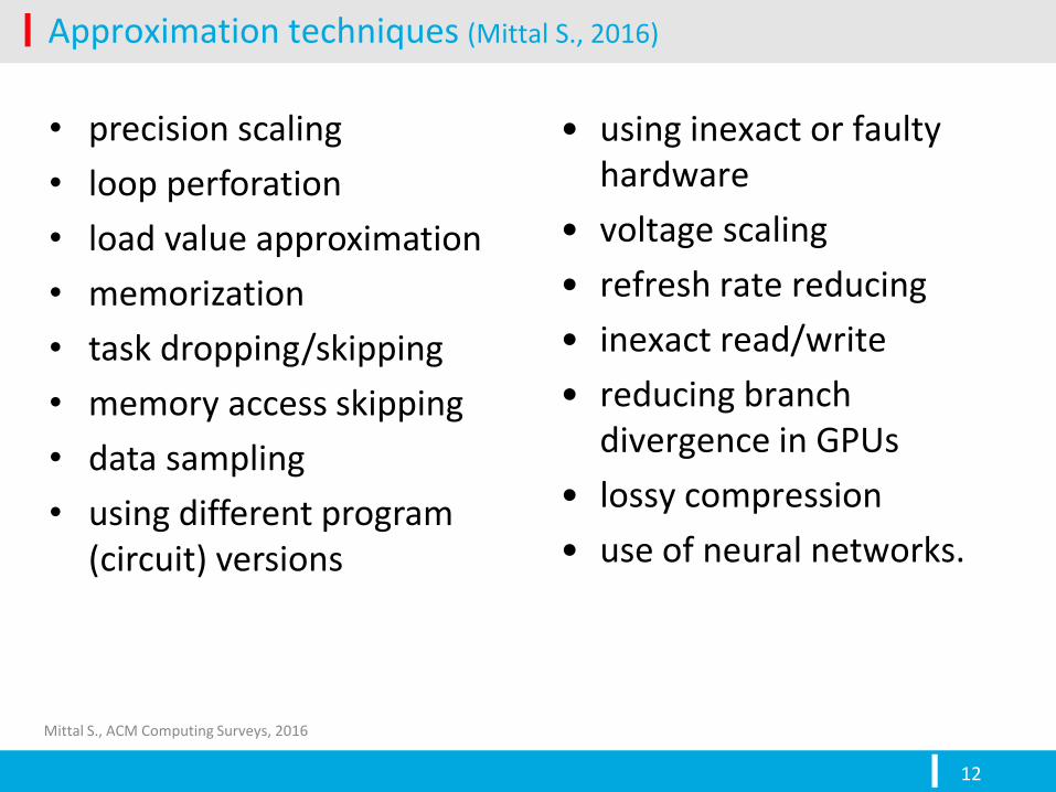
Approximation techniques (Mittal S., 2016)

12

• precision scaling

• loop perforation

• load value approximation

• memorization

• task dropping/skipping

• memory access skipping

• data sampling

• using different program (circuit) versions

• using inexact or faulty hardware

• voltage scaling

• refresh rate reducing

• inexact read/write

• reducing branch divergence in GPUs

• lossy compression

• use of neural networks.

Mittal S., ACM Computing Surveys, 2016

Approximate circuits

13

• Basic approximation techniques

• Timing induced approximations

• Functional approximation

• Approximation methodology

• Ad hoc (circuit-specific)

• Automated/systematic (circuit independent)

Timing induced approximations

14

• Design techniques

over-clocking

voltage over-scaling

path delay

# o

f p

ath

s

delay target

Pdyn = CVdd2 f

Vdd = 1.2V

path delay

# o

f p

ath

s Vdd = 1.2V

f 2f

Timing errors

speed

path delay

# o

f p

ath

s

delay target Vdd = 0.9V Timing errors

power

• Power reduction tricks

Assume: Accurate circuit D1 at

frequency f1

D1 is approximated to D2 which

can work at higher freq. f2 (f2 > f1)

But, D2 is operated at f1 with

lower Vdd => power saving

Courtesy of K. Roy

Functional approximation of digital circuits

15

Functional

approximation

Original design:

gate level / RTL / behavioral

Approximate circuit 𝑒𝑎𝑣𝑔 𝑓, 𝑓 =1

2𝑛 | int 𝑓 𝑥 − int(𝑓 𝑥 )

∀𝑥∈ℬ𝑛

|

Quality metrics,

constraints, data

Design methodology Ad hoc [e.g. Kulkarni et al.: J. Low Power Electronic, 2011]

Design automation methods (= some heuristics used)

SALSA (DAC 2012), SASIMI (DATE 2013), ABACUS (DATE 2014), ASLAN (DATE 2014), AIG-Rewriting (ICCAD 2016) …

Cartesian Genetic Programming (e.g. ICES 2013, IEEE Tr. on EC 2015, ICCAD 2016, DATE 2017, ICCAD 2017)

Automated functional circuit approximation: Classification

16

• Where is the approximation conducted? • Component (e.g. adder) / module (e.g. DCT) / application (e.g. video

compression)

• What is the level of abstraction? • transistor, gate, RTL, behavioral, abstract representation (e.g. SoP, BDD, AIG …)

• How is the circuit approximated? • truncation • pruning • component replacement (using a library of approximate components) • re-synthesis • others

• How are the candidate approximate circuits evaluated? • quality (at different levels of the application)

• simulation/probabilistic/formal-based methods • electrical parameters

• power, delay, area, …

• How is the approximation method evaluated? • The approximation methods are often heuristics! A proper statistical

evaluation is requested.

17

How to determine the error?

Error “estimation” • (Functional) circuit simulation • Probabilistic models, e.g. Li at al., DAC 2015

• applicable in very specific cases only

All possible input vectors

Approximate

circuit

1.3% 4.5%

Error = 3.1%

Exact error calculation • Exhaustive simulation – small problem instances only

• Analysis of Binary Decision Diagrams (ROBDDs)

• Worst-case error (M. Soeken et al., ASP-DAC’16)

• Average error (Vasicek et al., DATE’17 )

• Average Hamming distance (Vasicek, Sekanina, GENP’16)

• Not scalable for some circuits such as multipliers

• Transforming to SAT problem

• Worst case error

• Venkatesan et al. (ICCAD’11), Petkovska et al. (ICCAD’16), Ceska et. al. (ICCAD’17) …

• Not suitable if counting the number of solutions is requested.

On a fair comparison of automated approx. methods

18

• Common practice: The original circuit and approximate circuits created using a given method are compared -> not sufficient!

• A comparisons with other approximation methods is needed!

• Important assumptions for a fair comparison: • the original circuits are the same • the error is calculated using the same

method (simulation vs. exact) • electrical parameters are calculated using

the same tool and for the same technology library

• the time/resources for the approximation methods under investigation are the same

• the same statistically relevant values are reported (best, median, mean etc.)

8-bit multiplier approximation

power

erro

r

0

Method 1 (double time)

Method 1

Method 2

Method 3

original circuit

Ad hoc approximation approaches • adders • multipliers

19

H. Jiang, C. Liu et al., “A review, classification, and comparative evaluation of approximate arithmetic circuits,” J. Emerg. Technol. Comput. Syst., vol. 13, no. 4, pp. 60:1–60:34, Aug. 2017

Approximate adders (ad hoc)

20

• Speculative Adders • For a 128 bit adder, the probability that the carry propagation chain is

longer than 12 and 18 are 1% and 0.01%, respectively.

• Therefore, k bits are used to speculate the carry for each sum bit (k < n).

• Segmented Adders • An n-bit adder is divided in to a number of smaller k-bit sub-adders.

• The carry may be generated by using different methods.

• Carry-Select Adders • Multiple sub-circuits are used to compute the sum for different carry

values, and the result is selected by the carry of a sub-circuit.

• Approximate Full Adders

Han J. ESWEEK tutorial, 2017

Approximate adders (ad hoc)

21

Han J. ESWEEK tutorial, 2017

Approximate full adder

22 22

Approximate full adder – used JPEG

23

Approximate 16 bit adders

24

Han J. ESWEEK tutorial, 2017

16-bit unsigned adders

MRED (Mean Relative Error Distance) calculated with Monte Carlo simulation (100 M vectors)

ER (Error Rate)

PDP – Power Delay Product

STM CMOS 28 nm technology, 1V

PDF (fJ) PDF (fJ)

Erro

r R

ate

(%

)

Me

an R

ela

tive

Err

or

Dis

tan

ce (

10

-3)

Ad hoc approximation of multipliers: 2-bit multiplier

25

• Correct results for 15 out of 16 input combinations (almost 50% area reduction, lower delay).

• Used as a building block for larger multipliers and then in image processing applications.

accurate approximated

Error probability Dynamic power reduction for various frequencies

AxB 0 1 2 3 0 0 0 0 0

1 0 1 2 3

2 0 2 4 6

3 0 3 6 7

Kulkarni et al. Trading Accuracy for Power in a Multiplier Architecture, VLSI Design, 2011

MSB removed!

Approximate multipliers: Classification

26

Han J. ESWEEK tutorial, 2017

Classification Multiplier

Approximation in Generating partial products

Under-Designed Multiplier (UDM)

Approximation in the partial products

Broken Array Multiplier (BAM)

Error Tolerant Multiplier (ETM)

Approximate Wallace Tree Multiplier (AWTM)

Truncated Wallace Multiplier (TruMW)

Truncated Array Multiplier (TruMA)

Using approximate counters or compressors

Inaccurate Compressor based Multiplier (ICM)

Approximate Compressor based Multiplier (ACM)

Approximate Multiplier 1/2 (AM1/AM2)

Truncated AM1/AM2 (TAM1/TAM2)

Approximate Booth multipliers

Fixed-width Booth multipliers

Approximate multipliers: Evaluation

27

16-bit unsigned multipliers

MRED (Mean Relative Error Distance) calculated with Monte Carlo simulation (100 M vectors)

STM CMOS 28 nm technology, 1V

Han J. ESWEEK tutorial, 2017

PDF (fJ)

Me

an R

ela

tive

Err

or

Dis

tan

ce (

%)

Automated approximation methods

28

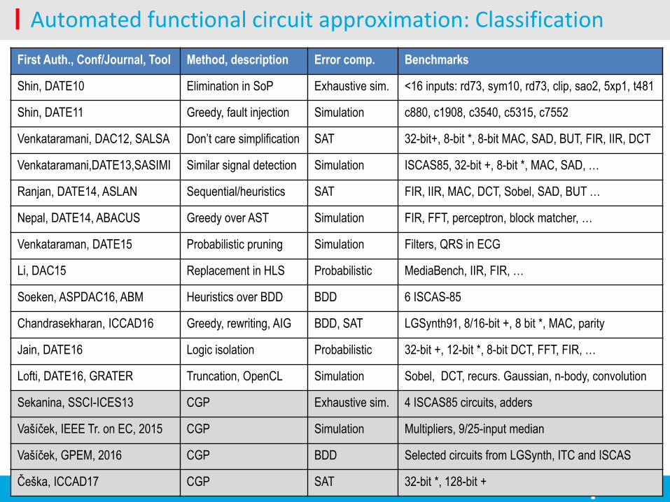
Automated functional circuit approximation: Classification

29

First Auth., Conf/Journal, Tool Method, description Error comp. Benchmarks

Shin, DATE10 Elimination in SoP Exhaustive sim. <16 inputs: rd73, sym10, rd73, clip, sao2, 5xp1, t481

Shin, DATE11 Greedy, fault injection Simulation c880, c1908, c3540, c5315, c7552

Venkataramani, DAC12, SALSA Don’t care simplification SAT 32-bit+, 8-bit *, 8-bit MAC, SAD, BUT, FIR, IIR, DCT

Venkataramani,DATE13,SASIMI Similar signal detection Simulation ISCAS85, 32-bit +, 8-bit *, MAC, SAD, …

Ranjan, DATE14, ASLAN Sequential/heuristics SAT FIR, IIR, MAC, DCT, Sobel, SAD, BUT …

Nepal, DATE14, ABACUS Greedy over AST Simulation FIR, FFT, perceptron, block matcher, …

Venkataraman, DATE15 Probabilistic pruning Simulation Filters, QRS in ECG

Li, DAC15 Replacement in HLS Probabilistic MediaBench, IIR, FIR, …

Soeken, ASPDAC16, ABM Heuristics over BDD BDD 6 ISCAS-85

Chandrasekharan, ICCAD16 Greedy, rewriting, AIG BDD, SAT LGSynth91, 8/16-bit +, 8 bit *, MAC, parity

Jain, DATE16 Logic isolation Probabilistic 32-bit +, 12-bit *, 8-bit DCT, FFT, FIR, …

Lofti, DATE16, GRATER Truncation, OpenCL Simulation Sobel, DCT, recurs. Gaussian, n-body, convolution

Sekanina, SSCI-ICES13 CGP Exhaustive sim. 4 ISCAS85 circuits, adders

Vašíček, IEEE Tr. on EC, 2015 CGP Simulation Multipliers, 9/25-input median

Vašíček, GPEM, 2016 CGP BDD Selected circuits from LGSynth, ITC and ISCAS

Češka, ICCAD17 CGP SAT 32-bit *, 128-bit +

Finding minterm complements to reduce # literals

30

Shin and Gupta: Approximate logic synthesis for error tolerant applications. DATE 2010

• The objective is to obtain designs that have a minimum number of literals for a given error rate threshold.

• Method: Identify minterm complements that produce an approximate circuit version that has the smallest number of literals for a given error rate threshold.

• Exhaustive search for simple functions, a heuristics approach for more complex functions.

𝑥1 𝑥2𝑥4 + 𝑥2𝑥3𝑥4 + 𝑥1𝑥2 𝑥3 𝑥4

𝑥2𝑥4 + 𝑥1𝑥3 𝑥4

𝑥1 𝑥2𝑥4 + 𝑥2𝑥3𝑥4

Original solution:

Approximation 1:

Approximation 2:

SASIMI: Substitute and Simplify

31

• Key Idea: Identify signal pairs (TS and SS) that are similar in functionality i.e. produce the same value for most of the inputs among signal pairs.

– Substitute one in place of the other

• Circuit becomes approximate

– Simplify the circuit: Logic Deletion & Downsizing

Original Circuit

TS = SS PDIFF ≈ 0 TS = !SS PDIFF ≈ 1 Difference Signal (DIFF)

Target Signal (TS)

Substitute Signal (SS)

Approximate Circuit

SS

Deleted gates

Downsized gates

Downsized gates

TS

S. Venkataramani, K. Roy, and A. Raghunathan: Substitute-and simplify: a unified design paradigm for approximate and quality configurable circuits, DATE’13, pp. 1367–1372

Courtesy of K. Roy

The signal probability calculation engine in Synopsys Power Compiler was used to obtain difference probabilities

SASIMI: Substitute and Simplify

32

S. Venkataramani, K. Roy, and A. Raghunathan, “Substitute-and simplify: a unified design paradigm for approximate and quality configurable circuits, DATE’13, pp. 1367–1372

Approximation-aware Rewriting of AIGs

33

Chandrasekharan, Soeken, Grosse, Drechsler. Approximation-aware Rewriting of AIGs for Error Tolerant Applications ICCAD 2016

2-bit adder

Heuristics: replace the cut

by constant 0

• Principle: allow AIG rewriting to change the functionality of the circuit without violating a predefined error bound.

• Rewriting (at the level of cuts on selected paths) takes a greedy approach.

• Worst-case error, bit-flip error and error rate determined exactly (formally).

• Evaluated: 8/16-bit adders, LGSYnth91, 8-bit multipliers, 32-bit parity, …

ABACUS: Approximations at Behavioral RT-level

34

ABACUS: Results

35

Nepal K. et al.: Automated High-Level Generation of Low-Power Approximate Computing Circuits, Trans. on Emerging Topics in Computing, 2017

Benchmark problems:

Results of evolutionary approximation:

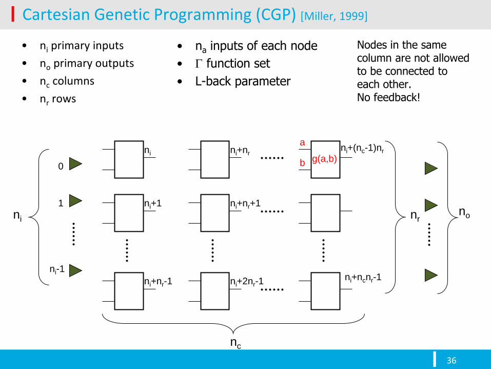
Cartesian Genetic Programming (CGP) [Miller, 1999]

36

• ni primary inputs

• no primary outputs

• nc columns

• nr rows

ni

ni+1

ni+nr-1

ni+nr

ni+nr+1

ni+2nr-1

ni+(nc-1)nr

• na inputs of each node

• function set

• L-back parameter

ni+ncnr-1

nr

nc

0

1

ni-1

ni no

Nodes in the same column are not allowed to be connected to each other. No feedback!

a

b g(a,b)

CGP: Representation for logic networks

37

Genotype (netlist):

na+1 integers per node; no integers for outputs;

Constant size: ncnr(na + 1) + no integers

Phenotype (directed acyclic graph circuit):

Variable size; unused nodes are ignored.

• CGP parameters • nr=3 (#rows) • nc = 3 (#columns) • ni = 3 (#inputs) • no = 2 (#outputs) • na = 2 (max. arity) • L = 3 (level-back

parameter) • = {NAND(0), NOR(1),

XOR(2), AND(3), OR(4), NOT (5)}

CGP: Fitness function for circuit design

38

target table:

Specification

(1-bit adder),

Typical fitness function (circuit functionality):

𝑓 = 𝑀𝑎𝑥 − 𝐻𝐷(𝑦𝑖

𝐾

𝑖=1

, 𝑤𝑖 )

Hamming distance

(between circuit response

and desired response)

The number of test vectors

Max = #outputs * 2#inputs (in our case 2 * 28 = 16)

K = 2#inputs for combinational circuits. Not scalable!!!

Additional objectives: • area (the number of gates)

• delay

• power consumption etc.

39

CGP: Mutation-based search

mutation

• Mutation: Randomly select h integers and replace them by randomly generated (but legal) values.

(for full adder)

40

CGP: Search algorithm (1 + )

; // or use conventional designs

41

CGP for circuit (functional) approximation

• Error-oriented (single-objective) method

• CGP gradually degrades a fully functional circuit

until a circuit with a required error is obtained.

Then, the area (and so power consumption) is

minimized for this error. Error

Are

a

Area

Erro

r

• Resources-oriented (single-objective)

method

• CGP is used to minimize the error, but only

limited resources (components) are provided,

insufficient for constructing a fully functional circuit.

Are

a

Pareto front

Error

• Multi-objective optimization

• All target parameters are optimized together.

Initial circuit Resulting circuit

Evolved library of 8-bit approx. adders and multipliers

42

• Comprehensive library of approximate arithmetic circuits

• 430 non-dominated adders (evolved from 13 accurate adders)

• 471 non-dominated multipliers (evolved from 6 accurate multipliers)

• Method: Multi-objective CGP with NSGA-II

V. Mrazek, R. Hrbacek, Z. Vasicek, L. Sekanina: EvoApprox8b, DATE 2017

Evolved library of 8-bit approx. multipliers

43

V. Mrazek, R. Hrbacek, Z. Vasicek, L. Sekanina: EvoApprox8b, DATE 2017

Evolved library of 8-bit approx. adders and multipliers

44

http://www.fit.vutbr.cz/research/groups/ehw/approxlib/

Approximate adders (430), exact adders (43)

Approximate multipliers (471), exact multipliers (28)

…………………………………………………………………………………………………………………………………………………

…………………………………………………………………………………………………………………………………………………

Synthesis results for 45 nm and 180 nm technology (Synopsys Design Compiler),

7 error metrics

45

Approximate neural networks on a chip

Approximations can be introduced in:

• ANN structure – pruning

• Data representation – compression.

• Memory – approximate cells and Load/Store

• Datapath

• Reducing data bit-width

• Multiplication in neurons and convolution layers

• approx. 30-50% of total power

• Activation function

• Sum function

∑wI

I0

I1

In

w0

w1

wn

Activation function

H1

H2

H3

H4

I1

I2

I3

O1

O2

Hidden layerInput layer Output layer

weights weights

Panda P. et al. Cross-layer approximations for neuromorphic computing: From devices to circuits and systems, DAC 2016

Approximate multipliers for Deep NNs

• Floating point (FP) used for training, fixed point (FX) for inference.

• FX: 8 – 16 bits are usually sufficient (e.g., 8-bit multipliers on TPU)

• Various approximate multipliers have been employed

• Multiplier-less multiplication (Alphabet Set Multiplier - ASM)

• 011001002 × X = (3X × 21) × 24 + (1X × 22) × 20

• Only a subset of weights is used

46

Sarwar S. et al. Energy-Efficient Neural Computing with Approximate Multipliers. ACM JETC 14(2), 2018

Case study: Evolution of approximate multipliers for CNNs

47

Scenario A:

• Multiplication 𝑚 𝑎, 𝑏 = 𝑎 ⋅ 𝑏 + Δ 𝑎, 𝑏

• Classification accuracy :

10.77%

MNIST dataset classification: 32x32 – 100 – 10 MLP network (classification accuracy 94.16% with accurate implementation). We introduced an approximate multiplier by adding a jitter function Δ(𝑎, 𝑏), resulting in a 5.2% error for multiplication.

Scenario B:

• 80% of multiplications are by 0

• Multiplication

𝑚′ 𝑎, 𝑏 = 0 𝑖𝑓 𝑎 = 0 ∨ 𝑏 = 0

𝑎 ⋅ 𝑏 + Δ 𝑎, 𝑏 𝑜𝑡ℎ𝑒𝑟𝑤𝑖𝑠𝑒

• Classification accuracy : 94.20%

Evolution of approximate multipliers for CNNs: Setup

48

Mrazek, Sarwar, Sekanina, Vasicek, Roy: “Design of power-efficient approximate multipliers for approximate artificial neural networks,” ICCAD 2016

Accurate multiplier – initial circuit (6) • CSAM RCA, CSAM RCA, RCAM, WTM CLA, WTM CSA, WTM RCA

Target errors: 𝜀 ∈ {0.5%, 1%, 2%, 5%, 10%, 15%, 20%}

CGP parameters • 𝑛𝑖 ∈ 14,22 ; 𝑛𝑜 ∈ 14,22 ; 𝑛𝑟 = 1; 250 < 𝑛𝑐 < 780

• Function set: {NOT, AND, NAND, OR, NOR, XOR, XNOR}

• Error constraints:

1. ∀𝑎, 𝑏: 𝑚 𝑎, 𝑏 − 𝑎 ∗ 𝑏 ≤ 𝜀 ⋅ 2𝑛𝑜

2. ∀𝑎: 𝑚 𝑎, 0 = 𝑚 0, 𝑎 = 0

• Fitness function:

𝐶 𝑚 = −𝐺𝑎𝑡𝑒𝑠𝐶𝑜𝑢𝑛𝑡(𝑚) 𝑖𝑓 𝑐𝑜𝑛𝑠𝑡𝑟𝑎𝑖𝑛𝑡𝑠 1 𝑎𝑛𝑑 (2) 𝑚𝑒𝑡,

−∞ 𝑜𝑡ℎ𝑒𝑟𝑤𝑖𝑠𝑒

Approximate multipliers (with 0 * x = 0) evolved with CGP

49

0

50

100

150

200

250

300

350

400

450

500

0% 0,50% 1% 2% 5% 10% 15% 20%

Power and area of 8 bit approximate multipliers

PWR μW AREA μm2

0

200

400

600

800

1000

1200

1400

0% 0,50% 1% 2% 5% 10% 15% 20%

Power and area of 12 bit approximate multipliers

PWR μW AREA μm2

Results of synthesis of sign-extended multipliers with Synopsys DC

• 45 nm technology

• Timing:

• 8-bit multipliers: 2.5 GHz

• 12-bit multipliers: 2 GHz

• Accurate multiplier was implemented in Verilog using standard * arithmetic operator

V. Mrazek, S. S. Sarwar, L. Sekanina, Z. Vasicek, and K. Roy, “Design of power-efficient approximate multipliers for approximate artificial neural networks,” Proc. IEEE/ACM Int. Conf. Computer-Aided Design, ICCAD 2016

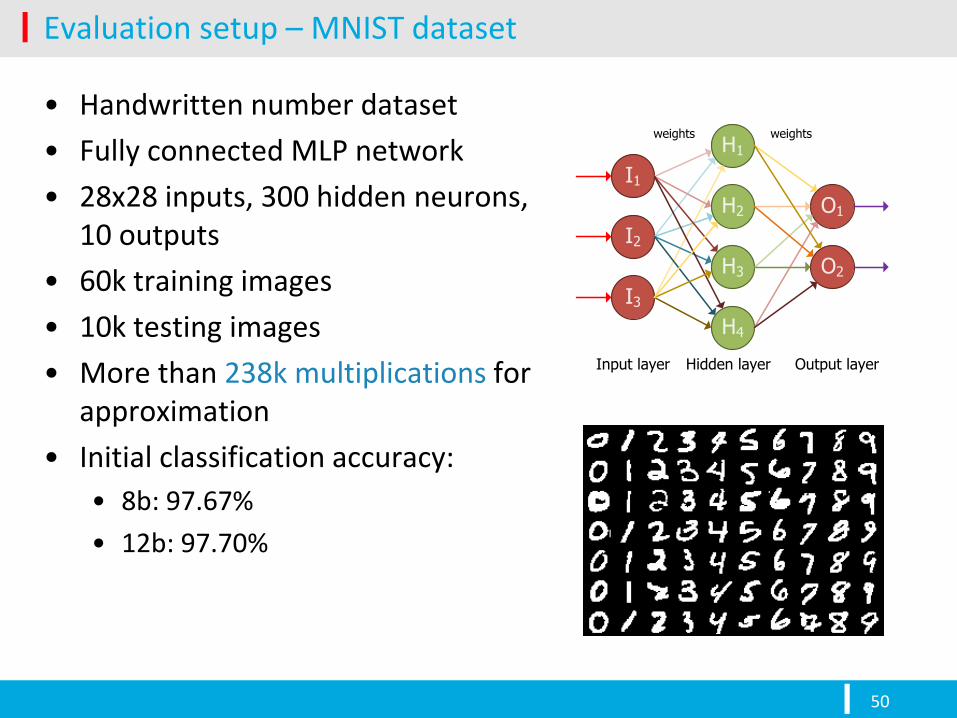
Evaluation setup – MNIST dataset

• Handwritten number dataset

• Fully connected MLP network

• 28x28 inputs, 300 hidden neurons, 10 outputs

• 60k training images

• 10k testing images

• More than 238k multiplications for approximation

• Initial classification accuracy:

• 8b: 97.67%

• 12b: 97.70%

50

H1

H2

H3

H4

I1

I2

I3

O1

O2

Hidden layerInput layer Output layer

weights weights

Evaluation setup – SVHN dataset

• Real-world data

• Convolutional LeNet NN

• 278,104 multiplications in 6 layers

• 73k training images

• 26k testing images

• Approximation introduced in L1,L3,L5 and L6 layers

• Initial classification accuracy: • 8b: 86.85%

• 12b: 86.90%

51

Input image32x32

6@28x28 6@14x14 16@10x10 16@5x5 120@1x1 10 values

L1 – Convolutional117,600 multiplications

L2 – Subsampling4,704 multiplications

L3 – Convolutional150,000 multiplications

L4 – Subsampling1,600 multiplications

L5 – Convolutional3,000 multiplications

L6 – Fully connected1,200 multiplications

Energy-efficient implementation of ANNs: Summary

52

Mrazek, Sarwar, Sekanina, Vasicek, Roy: “Design of power-efficient approximate multipliers for approximate artificial neural networks,” ICCAD 2016

-9%

-1%

-25%

-20%

-36%

-60%

70%

75%

80%

85%

90%

95%

100%

0% 0.50% 1% 2% 5% 10% 15% 20% {1} {1,3} {1,3,5,7}

Cla

ssif

icat

ion

acc

ura

cy o

f N

N

Approximation error ε of multipliers

Classification Accuracy and power reduction (in multiplication)

MNIST w=8

MNIST w=12

SVHN w=8

SVHN w=12

Multiplierless multiplication by Sarwar et al. DATE’2016

-20%

-50%

-30%

-43%

(8 bit)

(12 bit) Power

-57%

-66%

-77%

-70%

-82%

-85%

-91%

-86%

-91%

-87%

Non-linear image filters

53

filtered image (9-input median filter)

corrupted image (10% pixels, impulse noise)

original

Non-linear image filters: Approximation strategies

54

• Approximation of the comparator element – MONAJATI et al. Circuits, Systems, and Signal Processing, 34(10), 2015

• Approximation of the network (pruning)

– CGP used to find a network of N comparators minimizing the error w.r.t. the original median (consisting of K comparators), but resources are limited, i.e. N < K.

• Evolutionary image filter design from scratch

– CGP used to evolve an image filter showing a minimal error and cost. Filters are composed of elementary 2-input functions (min, max, +, logic functions over 8 bits).

Approximate median using CGP

55

• Median network (consisting of up to N operations) is represented by means of a one-dimensional array of N nodes.

• Each node can act as: identity (0), minimum (1), maximum (2) over 8 bits

• Each candidate solution is encoded using 3N + 1 integers.

• Fitness function (single objective)

e𝑟𝑟𝑜𝑟 = 𝑂𝑐𝑎𝑛𝑑𝑖𝑑𝑎𝑡𝑒 𝑖 − 𝑂𝑟𝑒𝑓𝑒𝑟𝑒𝑛𝑐𝑒(𝑖)

𝑖∈𝑆

• Example for a 3-input median:

Chromosome: 0, 2, 3; 3, 2, 0; 0, 2, 2; 5, 3, 1; 6, 1, 2; 7, 0, 0; 6, 8, 2; 8

Approximate median using CGP

56

Experimental setup

• (1+4) pop. size, no crossover, 5 % of the chromosome mutated

Median-9 Median-25

Inputs 9 25

Outputs 1 1

Generations 3 × 106 (3 hours) 3 × 105 (3 hours)

Training vectors 1 × 104 1 × 105

Exact solution (K) 38 operations 220 operations

Available nodes (N) 6 – 34 operations 10 – 200 operations

60% operation 20% operations original

Z. Vašíček and L. Sekanina. Evolutionary approach to approximate digital circuits design. IEEE trans. on Evol. Comp. 19(3), 2015

Approximate median: Distance error analysis

57

9-input median fully-working: 38 operations

25-input median fully-working: 220 operations

21% reduction

52% reduction

84% reduction

4.8%

95.2%

65.1%

24.6%

20.2% 13.4%

1.2%

23.8% 19.4% 12.3%

5.5% 14.3%

27% reduction

54% reduction

81% reduction

94.4%

45.9%

19.0%

V. Mrazek, Z. Vasicek and L. Sekanina. GECCO GI Workshop, 2015

Evolutionary design of image filters from scratch

58

Golden image - w Input image

Compare fitness

N

i

M

j

jiwjivfitness1 1

|),(),(|

N x M pixels

Output image - v

Sekanina L. Image Filter Design with Evolvable Hardware. LNCS 2279, 2002

59

Comparison of approximate median filters and evolved filters for salt

and pepper noise

∆ MF median filter ○ AMF adaptive median filter □ CWMF center weighted median filter ◊ EVO evolved filter (5x5) ⌂ BNK bank of 3 evolved filters (5x5) 9 3x3 kernel 25 5x5 kernel # xy approximation no. xy PSNR – mean PSNR on 30 images Synopsys Design compiler; 45 nm PDK All filters are pipelined with fmin = 1 GHz

Sekanina, Vasicek, Mrazek: Radioengineering 26(3), 2017

Testing of approximate circuits: New Challenges

• Instead of testing for all manufacturing defects, the goal is to test only for those that will lead to an error considered as not acceptable by the adopted Error Metrics.

• The main advantage: the test cost reduction

60

Traiola M. et al.: On the Comparison of Different ATPG Approaches for Approximate Integrated Circuits. IEEE DDECS 2018

Approximate FT circuits: TMR

61

61

b12

rd73

t481

SÁNCHEZ-CLEMENTE, A., J., ENTRENA, L., HRBACEK, R. a SEKANINA, L. Error Mitigation using Approximate Logic Circuits: A Comparison of Probabilistic and Evolutionary Approaches. IEEE Transactions on Reliability. 2016, 65(4), p. 1871-1883

Incorrect subspace: The subset of input vectors for which the correct circuit and approximate circuit produce different outputs.

F (under-approximation): Incorrect subspace is a subset of the on-set. 1 0 errors are produced

H (over-approximation) Incorrect subspace is a subset of the off-set. 0 1 errors are produced

At most one of the circuits is allowed to produce an incorrect output for any input vector.

Summary (1)

• Approximate computing is a hot topic!

• It is important as it addresses one of the most critical challenges of our society -- energy efficiency.

• The roots of approximate computing

• the need for low power & high performance computing

• high fabrication variability in current/future technology nodes

• many dominant applications are error resilient

• This tutorial is focused on approximate circuits and design methodologies.

• ad hoc circuit approximations

• automated circuit approximation methods

62

Summary (2)

• A lot of research is needed

• reliable quality (error) analysis methods -> Part II

• benchmarking methodology

• automated approximation methodologies

• scalable and systematic solutions for complex systems approximation across the computer stack

• What would be the impact of the approximation on:

• test

• reliability

• security

• trust?

63

References

• New Book Approximate Circuits: Methodologies and CAD, edited by S. Reda and M. Shafique, Springer, in press, 2019

• Selected tutorial and survey papers on Approximate Computing

• J. Han and M. Orshansky, “Approximate computing: An emerging paradigm for energy-efficient design,” in Proc. of the 18th IEEE European Test Symposium. IEEE, 2013, pp. 1–6

• H. Esmaeilzadeh, A. Sampson, L. Ceze, D. Burger, “Neural acceleration for general-purpose approximate programs,” Commun. ACM, 58(1): 105-115, 2015

• S. Mittal, “A survey of techniques for approximate computing,” ACM Computing Surveys, 48(4), 1–34, 2016.

• Q. Xu, T. Mytkowicz, N. S. Kim. “Approximate Computing: A Survey,” IEEE Design and Test, 33(1), 8-22, 2016.

• L. Sekanina, “Introduction to Approximate Computing”. IEEE International Symposium on Design and Diagnostics of Electronic Circuits, DDECS 2016

• Z. Vasicek, “Relaxed equivalence checking: a new challenge in logic synthesis”. IEEE International Symposium on Design and Diagnostics of Electronic Circuits, DDECS 2017

64

Acknowledgments

• Collaborators at FIT – Evolvable hardware group

• Zdeněk Vašíček, Michal Bidlo, Vojtěch Mrázek, Jakub Husa, David Grochol, Michal Wiglasz

• Former PhD students: Radek Hrbáček, Michaela Drahošová, Miloš Minařík

• Projects

• IT4Innovations Centre of Excellence – National supercomputing center

• Czech science foundation • Relaxed equivalence checking for approximate computing, 2016 –

2018

• Advancing cryptanalytic methods through evolutionary computing, 2016 - 2018

• Advanced Methods for Evolutionary Design of Complex Digital Circuits, 2014 – 2016

• Natural Computing on Unconventional Platforms, 2010 – 2013

• Brno University Technology

65

Thank you for your attention!