approximating risk aversion in decision analysis...

Approximating Risk Aversion

in Decision Analysis Applications

Craig W. Kirkwood

Department of Supply Chain ManagementArizona State UniversityTempe, AZ 85287-4706

(480) 965-6354Fax: (480) 965-8629

[email protected]

Forthcoming in Decision AnalysisCopyright c° INFORMS, 2002

April 2002

Abstract

This paper investigates the impact of risk aversion in decision analyses under uncertainty

with a single evaluation measure and presents a simple procedure for approximately ad-

dressing risk aversion in a way that is defensible for many decisions. Speci¯cally, a simu-

lation study is presented that leads to guidelines for determining when an expected utility

analysis should be conducted for a decision, rather than simply an expected value analysis,

and what form of utility function should be used for this expected utility analysis. The

simulation study shows that a sensitivity analysis using an exponential utility function

should be conducted for most decision analyses, but that this sensitivity analysis can often

establish, without requiring utility information from the decision maker, that no further

utility analysis is required. In addition, when further utility analysis is required, the sim-

ulation study shows that this can be done in a simple way using an exponential utility

function that will be accurate for many decision analyses. However, in situations where

there is equal or greater downside risk than upside potential a more detailed study of the

decision maker's utility function may be necessary.

Approximating Risk Aversion

in Decision Analysis Applications

1. Introduction

The concept of aversion to taking risks is important in the formal theory of decision

making under uncertainty, and expected utility analysis methods to address risk aversion

are presented in decision analysis textbooks (Clemen 1996, Kirkwood 1997). However,

when Corner and Corner (1995) analyzed published decision analysis applications over a

two decade period, they found that 67.0 percent of those applications used expected value

as the decision making criterion, and no formal analysis of risk aversion was reported in

these cases.

Practicing decision analysts report that using either expected value or expected utility

to evaluate alternatives often leads to similar decisions. For example, Howard (1988)

comments, \While the ability to capture risk preference [with a utility function] is an

important part of our conceptual view of decision-making, I ¯nd it is a matter of real

practical concern in only 5 percent to 10 percent of business decision analyses." However,

in some cases taking a risk aversion into account using a utility function does change the

results. (See, for example, Keefer 1991.) Therefore, not considering risk aversion can lead

to signi¯cant errors in some decisions.

The research presented below shows that an expected utility analysis will lead to

di®erent results from an expected value analysis for many decisions, but that a straight-

forward form of sensitivity analysis can identify when this will happen. Furthermore, even

when an expected utility analysis can result in changes to the decision analysis results, the

research shows that using a simple form of utility function which requires very little utility

elicitation from the decision maker will often be su±cient for an accurate analysis.

1

2. Previous Related Work

Consider decisions with a single evaluation measure x (for example, cost or pro¯t),

where the preferred alternative a is selected to maximize the expected utility E(uja) =Pu(x)p(xja), where p(xja) is the probability of outcome x given that a is selected and

u(x) is a utility function over x. Assume that preferences over this evaluation measure are

monotonically increasing so that u(x) is monotonically increasing over x. (The results pre-

sented below can be shown to also apply to situations where preferences are monotonically

decreasing.) This expected utility approach to analyzing decisions with uncertainty has

been widely applied (Corner and Kirkwood 1991), and it provides a defensible approach

for analyzing these decisions.

This section reviews several types of utility functions that have been applied, or pro-

posed for application, as well as empirical evidence about realistic parameter values for

these di®erent utility functions.

2.1. The Risk Tolerance Function and Utility Function Forms

For a utility function u(x), the risk tolerance function ½(x) = ¡u0(x)=u00(x), where

u0(x) and u00(x) are the ¯rst and second derivatives, respectively, of u(x), encodes the

decision maker's degree of risk aversion at each evaluation measure level x. Speci¯cally,

Pratt (1964) showed that for an uncertain alternative with small risk

xce ¼ ¹x¡ ¾2

2½(¹x); (1)

where ¹x and ¾2 are the expected value and variance, respectively, for the uncertain alter-

native, and the certainty equivalent xce is the level of x that is equally preferred to the

alternative.

Exponential Utility Function. Equation 1 shows that if the risk premium ¹x¡xce does

not change as a function of ¹x, then ½(¹x) must be a constant. When this condition holds a

2

decision maker is said to display constant risk aversion, and the utility function must be

either exponential or linear (Pratt 1964),

u(x) =

½¡sgn(½)e¡x=½; ½6=1x; otherwise,

(2)

where ½ is equal to the risk tolerance, and sgn(½) is the sign of ½.

Corner and Corner (1995) found that 27.5 per cent of the applications they reviewed

used exponential utility functions, while only 5.5 per cent used all other types of utility

functions combined or did not specify what utility function was used. (However, as noted

earlier, applications using only expected value outnumbered applications using any type

of utility function by a ratio of two to one.)

Power Utility Function. Pratt (1964) showed that when the risk premium is linearly

proportional to x, then the utility function must have either a power or log form

u(x) =

½sgn[(a¡ 1)=a]x(a¡1)=a; a6= 1log(x); otherwise

(3)

which has a risk tolerance function ½(x) = ax, where a is a constant. This condition

for ½(x) is called constant proportional risk aversion, and as is discussed below, there is

empirical evidence that this condition applies for some business decision makers.

Linear-Exponential Utility Function. A variety of other functional forms have been

suggested for u(x). See, for example, Bell (1995), Bell and Fishburn (2001), Brockett and

Golden (1987), Farquhar and Nakamura (1987, 1988), Hammond (1974), Harvey (1990),

Meyer and Pratt (1968), and Spetzler (1968). Of particular interest is a preference con-

dition called the one-switch rule. Preferences obey the one-switch rule if, for every pair

of alternatives whose ranking is not independent of asset position, there exists an asset

level above which one alternative is preferred, and below which the other is preferred. Bell

(1988) showed that if preferences 1) are decreasingly risk averse with respect to asset po-

sition [that is, ½(x) is monotonically increasing with respect to x], 2) obey the one-switch

3

rule, and 3) approach risk neutrality for small gambles as wealth increases, then the utility

function must have the linear-exponential form

u(x) = bx¡ e¡x=c (4)

for some positive constant parameters b and c. The three conditions required for the linear-

exponential utility function are intuitively reasonable, and therefore this utility function

is attractive from a theoretical standpoint, although it requires that two constants b and c

be determined, rather than the single constant that is required for either the exponential

or power utility function.

Mean-Variance Utility Models. In addition to the utility function forms discussed

above, mean-variance models of risk aversion similar to Equation 1 have been studied

and used for analysis of investment portfolios. See, for example, Jia and Dyer (1996),

Hlawitschka (1994), and Markowitz (1959, 1987, 1991). The quadratic utility function

that is implicitly assumed by a mean-variance utility model is increasingly risk averse as

the asset position increases (Pratt 1964), which is intuitively unattractive. As part of the

simulation study conducted for this paper, the accuracy of Equation 1 to approximate risk

aversion was analyzed, and this approximation was found to be substantially less accurate

than the approach that is recommended. Hence mean-variance utility models are not

considered further in this paper.

Exponential, power, or linear-exponential utility functions will have either a risk averse

or risk seeking risk attitude for all positive levels of x. Experiments have shown that un-

aided decision makers can display a risk averse attitude for some levels of x and a risk

seeking behavior for other levels (Clemen 1996, pages 510{511, Fishburn and Kochen-

berger 1979, Laughhunn, Payne, and Crum 1980), but utility functions with this behavior

are rarely reported in the decision analysis application literature and are not considered

further.

4

2.2. Decision Maker's Accustomed Budget and Risk Aversion

Empirical studies of business people's risk attitudes have found that utility func-

tions are generally nonlinear for the individuals studied. [See, for example, Green (1963),

Laughhunn, Payne, and Crum (1980), MacCrimmon and Wehrung (1986), Shapira (1995),

Spetzler (1968), and Swalm (1966).] The degree of risk aversion that was displayed in these

studies typically depended on how large the risks were relative to the decision maker's ac-

customed budget. For example, Spetzler (1968) assessed utility functions for 36 executives

in a company with total annual sales of $2,000 million, annual after-tax earnings of $100

million, and a capital investment budget of $90 million per year. Initially, he used hypo-

thetical alternatives involving either a $3 million or a $50 million investment. After the

¯rst round of assessments, the executives requested that the amounts be reduced by a

factor of ten to $300,000 and $5 million, and they noted that $300,000 investments were

\rather common," while $5 million investments occurred between four and eight times

a year. Thus, the initially speci¯ed $3 million and $50 million amounts were very large

relative the typical budgets that the executives addressed.

As a second example, Swalm (1966) asked 100 executives to specify the maximum

single amount that they might recommend be spent in any one year. (These amounts

ranged from $50 thousand to $40 million.) He then speci¯ed outcomes for utility function

assessments as a proportion of this amount, and he found that the utility functions of the

various executives, when expressed in these terms, were roughly comparable. Thus, the

executives appeared to be assessing risks relative to the investment amounts with which

they usually worked.

Also, MacCrimmon and Wehrung (1986) studied 509 executives and speci¯ed utility

function assessments in terms of the rate of return on an investment of half of their ¯rm

or division's annual capital expenditure budget. These budgets ranged from less than

$300,000 to over $1,500 million, with half over $12 million. A substantial portion of the

executives refused to risk half of their annual budget unless the probability of loss was

5

very low, and some refused to risk it even when risk of loss was very low. Once again in

this example, the executives appeared to be judging risks in relation to their accustomed

budget amounts.

Howard (1988) proposed values of risk tolerance for corporate decision making that

are proportional to net sales, net income, or equity. Speci¯cally, his experience suggests

setting the risk tolerance at six per cent of sales, one to one and a half times net income,

or one-sixth of equity. (These numbers are based on studies with companies in the oil

and chemical industry.) McNamee and Celona (1990, pp. 122{123) add to this list a

ratio of market value to risk tolerance of one-¯fth. They also comment that \the ratio

of risk tolerance to equity or market value usually translates best between companies in

di®erent industries." In practice, the net sales, net income, equity, and market value for a

company will generally be positively correlated, and they are each measures of the \size"

of a company. Thus, Howard's suggested method for approximating the risk tolerance

is another indication that executives judge risks in relation to their accustomed budget

amounts.

These empirical studies support the view that attitude toward taking business risks

is related to the size of the budget or assets which the decision maker typically addresses.

This characteristic is consistent with constant proportional risk aversion and possibly the

linear-exponential utility function, but not with constant risk aversion, even though the

constantly risk averse exponential utility function is the most commonly used form in

published applications that use utility functions. The remainder of this paper investigates

whether using expected value or an exponential utility function, as is often done in decision

analysis practice, can lead to signi¯cant errors.

3. Study Approach

The impact of the utility function form on decision analysis results is investigated

in this paper using simulation. Randomly generated uncertain alternatives selected to

6

be representative of real-world decision alternatives were ranked using exponential, power,

and linear-exponential utility functions with parameters for these utility functions speci¯ed

to represent realistic attitudes toward risk taking. Di®erent pairs of alternatives meeting

the speci¯ed conditions were randomly generated, and these were ranked using expected

value and the three di®erent utility function forms. Statistics were collected regarding the

di®erences in the results from using the di®erent functions. These statistics were then used

to investigate the losses resulting from ignoring the decision maker's risk aversion (that

is, using expected value to rank alternatives), and also the losses resulting from using an

inaccurate form for the utility function.

The studies cited above indicate that a decision maker's attitude toward risk taking

is related to the budget or assets that he or she is used to addressing. Therefore, the

remainder of this paper will assume that the evaluation measure x is speci¯ed as a pro-

portion of the planning asset position for the decision maker, where x = 1 corresponds

to that planning asset position. The concept of a planning asset position can be clari-

¯ed with examples. First, consider personal investment decisions for an individual aged

forty-¯ve with $100,000 in assets outside of a contributory tax-deferred pension plan, and

with $500,000 invested in the tax-deferred pension plan. That individual might consider

$100,000 to be his or her planning asset position for decisions with uncertainty related to

assets that might be needed within the next ten years. However, $500,000 might be the

appropriate planning asset position for decisions related to assets that will not be used

until retirement.

As a second example, a corporation considering major strategic capital investments,

such as a semiconductor fabrication facility costing $2,000 million, might view corporate

equity or market value as an appropriate planning asset position. On the other hand,

a divisional director whose division contributes ¯ve per cent of the overall corporate net

income might consider ¯ve per cent of the overall corporation equity or market value to

be his or her planning asset position.

7

3.1. Utility Functions

A starting point for estimating realistic parameter values for the utility functions used

in this study is provided by considering a hypothetical uncertain alternative with equal

chances of yielding either a positive amount R or a negative amount R=2. For a decision

maker with an exponential utility function, if R is adjusted so that the decision maker is

indi®erent between accepting or not accepting the alternative, then R is approximately

equal to the decision maker's risk tolerance ½. (The error in ½ determined using this

approximation is about four per cent.)

For example, if a decision maker has a risk tolerance of 1, then he or she is approx-

imately indi®erent between accepting or not accepting an alternative with equal chances

of doubling his or her planning assets or losing half of these planning assets. Given the

results found by MacCrimmon and Wehrung (1986), it seems unlikely that many business

executives would be willing to take this high of a risk. On the other hand, with a risk

tolerance of 0.1, a decision maker is approximately indi®erent between accepting or not

accepting an alternative with equal chances of yielding a one-tenth increase in his or her

planning assets or losing one-twentieth of these assets. It seems likely that many business

decision makers would accept this alternative, and hence, a risk tolerance at least as large

as 0.1 seems to be realistic for business decision makers.

Based on the discussion in the preceding paragraph, the four sets of utility function

parameters shown in Table 1 were used in the simulation study. These parameter sets were

selected so that the risk tolerance at x = 1 (that is, at the decision maker's planning asset

position) is equal to 0.1, 0.2, 0.3, and 0.5, respectively.

Because the linear-exponential utility function has two parameters, it is necessary to

specify more than just the risk tolerance at x = 1 to determine the parameters b and c.

The values of b and c shown in Table 1 were determined using the following reasoning:

The risk tolerance for the exponential utility function is the same regardless of the value

of x, while the risk tolerance for the power utility function is a linear function of x. Thus,

8

for the exponential utility function, the risk tolerance is the same at x = 0:5, x = 1, and

x = 1:5, but for the power utility function, the risk tolerance at x = 1 is twice the risk

tolerance at x = 0:5, and similarly the risk tolerance at x = 1:5 is three times the risk

tolerance at x = 0:5. To provide a linear-exponential utility function with risk properties

that are between the properties for the exponential and the power utility functions, the

parameters of the linear-exponential utility function were determined such that the risk

tolerance at x = 1:5 isp

3 (that is, 1.7321) times the risk tolerance at x = 0:5. (Other

parameter sets were also studied for the linear-exponential utility function, as discussed in

Appendix A.1.)

3.2. Preliminary Graphical Analysis

Insight into the three utility function forms discussed above can be gained from Fig-

ures 1 and 2. In these ¯gures, the curve designated \Linear" represents using expected

value as the decision criterion, \Exponential" represents the exponential utility function

in Equation 2, \Power" represents the power utility function in Equation 3, and \Linear-

Exponential" represents the linear-exponential utility function in Equation 4. Figure 1

shows plots of the utility functions using Utility Parameter Set 2 in Table 1. There are

two arbitrary scaling constants associated with any utility function, and in Figure 1 these

have been set so that both the value and derivative of each utility function are equal to

one at x = 1. Figure 2 shows plots of the inverse of the risk tolerance function 1=½(x),

which is called the risk aversion function, for these utility functions. (The inverse of the

risk tolerance function associated with using expected value is equal to zero.)

Since Utility Parameter Set 2 is fairly risk averse relative to the planning asset position,

di®erences among the risk properties of the utility functions should show up strongly in this

case. Figure 1 seems to indicate that the three utility functions, while di®ering substantially

from the linear case, do not di®er much from each other. In particular, it appears from

this graph that the three utility functions have almost identical properties for x > 1, and

9

that the exponential and linear-exponential utility function are almost identical over the

entire range that is shown.

However, Pratt (1964) demonstrated that ½(x) more clearly portrays risk aversion

properties than u(x) because risk aversion is a direct function of ½(x) but only indirectly

a function of u(x). In particular, Equation 1 shows that the risk premium for a small

risk alternative is proportional to the inverse of the risk aversion function evaluated at the

expected value of the alternative. Keeping this in mind, the plots of 1=½(x) in Figure 2

show a di®erent picture of the risk aversion properties of the Figure 1 utility functions than

what appears to be true from Figure 1. In particular, Figure 2 shows that the inverses of

the risk tolerances associated with the exponential, power, and linear-exponential utility

functions are diverging as x increases above one, and therefore the risk premiums calculated

for small risk alternatives using these utility functions will become increasingly di®erent

as the expected values of the alternatives increase above one. For example, 1=½(2) = 5:0

for the exponential utility function, 2.5 for the power utility function, and 0.47 for the

linear-exponential utility function. Thus, the exponential utility function has twice the

risk premium for a small risk alternative with ¹x = 2 as the power utility function, and

5:0=0:47 = 10:6 times as great a risk premium as the linear-exponential utility function at

¹x = 2.

The di®erences for x < 1 are also substantial. For example, 1=½(0:5) = 5:0 for the

exponential utility function, 10.0 for the power utility function, and 5.2 for the linear-

exponential utility function. Thus, the di®erence between risk premiums using the power

utility function and risk premiums using the other two utility functions is approximately

a factor of two for ¹x = 0:5. Overall, the plots in Figure 2 raise the possibility that the

exponential utility function is not an accurate approximation for the other two utility

function forms in decision making, and this is investigated in more detail below.

10

3.3. Probability Distributions for Decision Alternatives

For the simulation study, four types of probability distributions were used to repre-

sent realistic decision alternatives. For the ¯rst set of simulation cases, each uncertain

alternative was represented by a shifted and scaled beta distribution, which is a °exible

continuous probability distribution that can assume a variety of di®erent shapes depending

on its parameters ® and ¯. The standard beta distribution over the range from zero to

one, f(x) = ¡(® + ¯ + 2)x®(1 ¡ x)¯=[¡(® + 1)¡(¯ + 1)], ® > ¡1, ¯ > ¡1, was shifted

to cover a speci¯ed range and then scaled to integrate to one over the speci¯ed range.

To simulate realistic decision alternatives, the beta distribution was also restricted to be

two-tailed. That is, ® and ¯ were restricted to be positive so that the distribution was

unimodal with an interior mode. (Simulation runs were also made without this restriction,

and the results were similar to those reported below.)

For the second set of simulation cases, each alternative was represented by a shifted

gamma distribution f(x) = (x¡ º)® exp[¡(x¡ º)=¯]=[¡(®+ 1)¯®+1], ® > ¡1, ¯ > 0, and

x > º. This set of cases was studied to verify that the results with the beta distribution

were not dependent on the speci¯c characteristics of that distribution

For the third set of simulation cases, each alternative was represented by a discrete

distribution with two possible outcomes (that is, a binary discrete distribution). This set

of cases was used to investigate whether the results for the beta and gamma distribution

runs also hold when the decision alternatives can have only two possible outcomes.

For the fourth set of simulation cases, each alternative was represented by a discrete

distribution with ¯ve possible outcomes which were generated based on the beta distribu-

tion. This set of simulation runs was used to investigate whether the results for the binary

discrete case might change as the number of possible discrete outcomes was increased.

The ¯fth set of simulation cases investigated whether the results for the ¯rst four sets

of simulation cases depend on the fact that the alternatives are discrete for those cases.

In particular, following Clyman, Walls, and Dyer (1999), a binary discrete \prospect"

11

was considered where the decision is what portion of this uncertain prospect to take.

Speci¯cally, suppose that xh and xl are the higher and lower of the two possible outcomes,

respectively, for this binary prospect, and ph is the probability that xh will occur. The

decision is what portion f to take of the prospect relative to the planning asset position of

x = 1, where the expected ¯nal asset position from taking a portion f is 1+ph£f £ (xh¡

1)+(1¡ph)£f£ (xl¡1). It is straightforward to show that the maximum expected value

for this alternatives will be obtained with either f = 0 or f = 1, depending on whether

the expected value of the entire prospect is greater than one. However, partial portions of

the prospect (that is, 0 < f < 1) can be optimal for nonlinear utility functions.

Finally, a sixth set of simulation cases investigated whether the \right-skew" charac-

teristics of the probability distributions in the earlier simulations might impact the results.

As is discussed in the next section, the parameters for the various simulation cases in the

¯rst ¯ve sets of simulations were set so that the probability distributions had longer tails

to the right than to the left (that is, these distributions were \right skewed" and hence

had more upside potential for gain than downside risk of loss). This ¯nal set of simulation

cases used beta distributions, but unlike the ¯rst set of simulation cases, the parameters

for these beta distributions were set so that the distributions were either symmetric or had

longer tails to the left than to the right (that is, were \left-skewed" and hence had more

downside risk of loss than upside potential for gain).

3.4. Parameter Values for the Probability Distributions

In order to provide comparability for the simulations results obtained using the dif-

ferent types of distributions, certain properties of the distributions were matched among

the di®erent distribution types. Speci¯cally, to the extent that this applied for the various

distribution types, the following properties of the di®erent distribution types were matched

in the simulation procedure: 1) range, 2) expected value, and 3) variance. For each dis-

tribution type that was studied, it is straightforward to convert from values of these three

12

properties to the parameters that determine a speci¯c distribution. The rationale for the

speci¯c values that were used for range, expected value, and variance is discussed in the

next paragraph.

Beta distributions. For the ¯rst set of simulation runs using beta distributions to

represent the simulated alternatives, four sets of parameters were used to randomly gen-

erate pairs of alternatives for the simulation runs, as shown in Table 2. Each parameter

set occupies two rows in this table. The ¯rst of the two rows, marked \Low," shows

the lowest value allowed in the simulation replications for each parameter, and the sec-

ond row, marked \High," shows the highest allowed value. The column marked \Range"

shows the range of allowed evaluation measure levels for the shifted-scaled beta distribu-

tion, the column marked \Expected Value" shows the range of allowed expected values for

the shifted-scaled beta distributions, and the column marked \Standard Deviation" shows

the range of standard deviations allowed for these distributions. All of these parameter

sets were selected to generate probability distributions with more upside potential for gain

than downside risk of loss (that is, to be right-skewed) so as to match what is typically

encountered in practice.

The speci¯c beta distribution for a particular simulation replication was generated

by randomly selecting an expected value using a uniform probability distribution over the

range speci¯ed in the \Expected Value" column of Table 2, and also randomly selecting

a standard deviation using a uniform probability distribution over the range speci¯ed in

the \Standard Deviation" column of Table 2. The generated expected value and standard

deviation were then used to determine values of ® and ¯ for the beta distribution. The

resulting values of ® and ¯ were then checked to make sure they were both positive. If

not, the probability distribution was not two-tailed, and it was discarded and another one

was generated. Once two acceptable beta distributions were generated, the error analysis

discussed in Section 3.5 was carried out and statistics were collected for analysis at the

end of the simulation run.

13

The parameter ranges shown in Table 2 are for the ¯nal outcome after the uncertainty

is resolved, net of any cost to purchase the simulated alternative. That is, the ranges are for

the ¯nal asset position resulting from the simulated alternative. To understand the basis

for the parameter sets shown in Table 2, keep in mind that the evaluation measure is the

¯nal asset position relative to a starting planning asset position of x = 1. In many business

decisions, serious consideration will usually only be given to alternatives that have positive

expected values, and therefore the intervals for both the ranges and expected values in

all of the simulation cases are biased toward values of x greater than one. For example,

in Simulation Case 1, the range for the expected value is from 0.98 to 1.04, and so the

mean of the expected values that are generated in the simulation replications will be 1.01,

and hence on average the alternatives that are generated for the replications in Simulation

Case 1 will have expected values for the ¯nal asset position that are greater than the

planning asset position (x = 1) of the decision maker. Similarly, the interval for the range

was set with some bias toward levels greater than x = 1 to agree with the way that the

expected values were generated. The range for the standard deviation was set so that the

distribution would represent situations where there was signi¯cant uncertainty relative to

the expected variation from the planning asset position, but where the standard deviation

was not so large that it would be di±cult to generate two-tailed beta distributions.

Parameter cases further down in Table 2 have a wider range of possible evaluation

measure levels and greater possible variation in the expected values and standard deviations

of the generated decision alternatives. The ¯rst two sets of values might be regarded as

\normal" types of risks, while the last two sets have more signi¯cant risks, with the last

set posing the possibility of losing as much as sixty percent of the planning asset position.

In addition to the cases in Table 2, several variations were also studied, and results for

these variations were similar to those reported below for the Table 2 cases.

Gamma distributions. The parameters shown in Table 2 were also used to generate

gamma distributions for the gamma distribution simulation runs, with º in the shifted

14

gamma distribution set equal to the Range Low numbers in Table 2. Since there is no

limit to the upper tail of a gamma distribution, the Range High numbers in Table 2 were

not used for the gamma distribution simulations.

Binary discrete distributions. For the binary discrete distribution simulation runs,

twenty di®erent distribution parameter sets were used to generate two-outcome discrete

alternatives. Speci¯cally, the four sets of expected value and standard deviation parameters

shown in Table 2 were used in combination with ¯ve di®erent probabilities for the higher

outcome of the two possibilities: 0.10, 0.25, 0.50, 0.75, and 0.90. For each simulation

run, a particular value of this probability was speci¯ed, and then values were randomly

generated for the expected value and standard deviation using the procedure discussed

above for the beta distribution runs. These values were then used to determine x-levels

for the two possible outcomes. For each generated alternative, if the lower outcome was

less than zero the alternative was discarded and another one was generated until two valid

binary distributions were created.

Five-outcome discrete distributions. Two ¯ve-outcome discrete distribution were

generated for each simulation run as ¯ve-outcome approximations to the distributions

used for the beta distribution runs. This was done by dividing the range of the beta

distribution into ¯ve equal intervals and ¯nding the height of the beta distribution at the

mid-value of each interval. The resulting ¯ve values were rescaled to sum to one and used

as probabilities for the mid-values, which were taken as the ¯ve possible discrete outcomes.

Continuous alternatives. For the continuous alternative simulation runs, the proce-

dure discussed above for the binary discrete simulations was used to generate each binary

discrete distribution. Then an exhaustive grid search was used to determine the optimal

portion f of this \prospect" using each of the di®erent utility functions.

Symmetric and left-skewed beta distributions. All of the probability distribution cases

in Table 2 have upper limits on the ranges of possible values that are further from any

of the possible simulated expected values than the lower limits on the ranges of possible

15

values. Hence, all of the probability distributions generated in simulations using the Table

2 parameters will be right-skewed and therefore have more upside potential for gain than

downside risk of loss. To investigate whether using right-skewed distributions was impact-

ing the results, three additional sets of simulation runs were made using beta distributions.

Each set of simulation cases used a set of probability distribution parameters that was a

modi¯cation of the parameters for the simulation cases shown in Table 2 so that direct

comparisons could be made with the results from the earlier set of beta simulation cases.

In particular, four di®erent simulation cases were used for each set of simulation runs that

paralleled the four cases in Table 2.

In each of these simulation cases, the same ranges were used for the Standard Deviation

as shown in Table 2, but the ranges were modi¯ed for the Range and the Expected Value.

In the ¯rst set of these simulation runs, the lengths of the ranges of variations shown in

Table 2 for Range and Expected Value were kept the same, but the locations of these ranges

of variation were shifted to be symmetric around the planning asset position, x = 1. Thus,

the modi¯ed version of Simulation Case 1 was set with the Low for the Range at 0.85 and

the High of 1.15, and with the Low for the Expected Value at 0.97 and the High at 1.03.

Similarly, the modi¯ed version of Simulation Case 2 was set with the Low for the Range

at 0.70 and the High at 1.30, and so forth. Thus, this set of simulation cases tended to

generate relatively symmetric probability distributions which therefore had equal upside

potential for gain and downside risk of loss.

For the second set of these simulation runs, the ranges of variation for both the

Expected Value and Standard Deviation was kept as shown in Table 2, but the range

of variation for the Range was \mirror-imaged" around x = 1 so that there was more

downside risk than upside potential. For example, Table 2 shows the range of variation for

the Range in Simulation Case 1 running from 1 ¡ 0:1 = 0:9 to 1 + 0:2 = 1:2. Therefore,

in the corresponding modi¯ed simulation case investigated here, the range of variation

was set from 1 ¡ 0:2 = 0:8 to 1 + 0:1 = 1:1. The range of variation for Range was

16

set in the same way for the other three cases, except that using this procedure for the

modi¯ed version of Simulation Case 4 would result in a range of variation for Range from

1 ¡ 1:2 = ¡0:2 to 1 + 0:6 = 1:6. Values of x less than zero are not typically meaningful

since they represent situations where more than the total planning assets would be lost.

To address this di±culty, two slightly di®erent variations were investigated for this case,

one where the range of variation for Range was truncated at x = 0 (hence yielding a range

of variation from 0 to 1.6) and another where the upper end of the range of variation was

adjusted to keep the total length of the range the same as shown in Table 2 (hence yielding

a range of variation for Range from 0 to 1.8).

The second set of simulation runs described in the preceding paragraph had expected

values greater than the current asset position but probability distributions that were left-

skewed so there was more downside risk than upside potential. (That is, while the expected

outcome from the alternatives was an increase in the decision maker's asset position, there

was a possibility of decreasing that asset position more than it could be increased.) To

investigate situations where the expected value of the simulated alternatives is also biased

toward reducing the decision maker's asset position, a third set of simulation runs was

made. In this set of runs, not only were the ranges of variation for the Range mirror-

imaged relative to the ranges shown in Table 2, but the ranges of variation for the Expected

Value were also mirror-imaged. Thus, for the modi¯ed simulation case corresponding to

Simulation Case 1 in Table 2, the range of variation for the Expected Value was set from

a Low of 1 ¡ 0:04 = 0:96 to a High of 1 + 0:02 = 1:02. While most business decision

making situations would hopefully not include such a set of negative alternatives, this

modi¯ed set of simulation runs investigated the performance of di®erent approximations

in this situation.

17

3.5. Performance Measures

Two di®erent types of performance measures were used to assess the accuracy of

expected value and the exponential utility function in situations where the actual utility

function was assumed to have a di®erent form.

Decision di®erences. When investigating how well an approximate decision analy-

sis procedure performs, a useful performance measure is the proportion of cases where

the approximate procedure identi¯es the same preferred alternative as the exact analysis

procedure. This is a useful performance measure because if the approximate procedure

selects the same alternative as the exact procedure then numerical errors in the calculated

numbers are not important from a decision-making standpoint. For continuous decision

alternatives, there is an additional complexity since the selected portion f can be incorrect

by di®ering amounts. Therefore, with continuous alternatives an appropriate measure of

decision di®erences is the di®erence between the optimal portion f of the prospect de-

termined using the approximate procedure and the optimal portion determined using the

exact analysis procedure.

Certainty equivalent di®erences. A second performance measure for judging the

accuracy of an approximation is the loss in certainty equivalent from using that approxi-

mation when it selects a less preferred alternative. The seriousness of selecting a di®erent

preferred alternative from the exact analysis depends on the di®erence between the cer-

tainty equivalent of the (incorrectly) selected alternative and the certainty equivalent of

the actual preferred alternative, both calculated using the assumed correct utility function.

When this di®erence is small, the incorrectly selected alternative is almost as valuable as

the actual most preferred alternative, and hence the loss from selecting the less preferred

alternative is small.

18

3.6. Implementing the Simulation Procedure

Each simulation run consisted of a speci¯ed number of replications using one of the

four Utility Parameter Sets speci¯ed in Table 1 and one of the probability distribution

types speci¯ed in Section 3.3. For each simulation run, one of the four probability distri-

bution parameter generation cases speci¯ed in Table 2 (or one of the modi¯cations to these

discussed above) was used to generate speci¯c parameters for the probability distributions.

For each replication within those simulation runs that analyzed discrete alternatives, the

speci¯c parameters for two probability distributions representing two di®erent simulated

discrete alternatives were selected using the procedure speci¯ed in Section 3.4. Then, for

each of the two alternatives that was generated, the expected value was calculated as well

as the certainty equivalents using exponential, power, and linear-exponential utility func-

tions. Values were then calculated for the performance metrics discussed in Section 3.5. At

the end of each simulation run, summary statistics were determined for each performance

measure, as discussed below in Section 4.

The procedure for the simulation runs that analyzed continuous alternatives was sim-

ilar except that only one probability distribution needed to be generated, and the optimal

portion f of the prospect was calculated four di®erent times using, in sequence, expected

value and each of the three utility function types. The di®erences among the optimal por-

tions as determined using each of these were then analyzed using the performance measures

discussed in Section 3.5.

This simulation procedure was implemented in the Pascal programming language us-

ing the Delphi for Win32 compiler, Version 10.0, running under Windows (Borland In-

ternational, Inc., 1997). Random numbers to select the parameters for the probability

distributions used in the simulation were generated using Bratley, Fox, and Schrage's

(1983) well-tested 32-bit UNIF random number generator.

19

For the beta distributions, expected utilities were calculated by numerical integration

using an equal interval approximation for the shifted-scaled beta distribution with the mid-

value of each interval used to represent the interval. One thousand intervals were used for

most of the integrations. A similar procedure was used for the gamma distributions.

(Since the gamma distribution does not have a pre-speci¯ed upper limit, the integration

was carried out over the range from the speci¯ed lower limit to ten standard deviations

above the expected value.)

One thousand replications were used for most simulation runs, but several cases were

run using 10,000 replications, and the results were almost the same. (As discussed in Sec-

tion 3.5, one performance measure to evaluate the various approximations is the proportion

of cases where a speci¯ed approximation selects the correct preferred alternative. For a

proportion estimated by 1,000 simulation replications, the largest 95% con¯dence interval

has a width of approximately §0:03, and the largest 99% con¯dence interval has a width

of approximately §0:04.)

For the continuous alternative simulations, an exhaustive grid search with 2,000

equally spaced grid points was used to determine the optimal portion f of the uncertain

prospect for each utility parameter set.

4. Simulation Results

Over 675 simulation cases, each with at least 1,000 replications, were analyzed. This

section presents quantitative results for representative simulation cases and qualitatively

discusses the results for other cases.

4.1. Accuracy of Expected Value (Beta Distributions)

Tables 3 through 5 summarize results for beta distribution simulation runs that tested

the accuracy of using expected value to rank pairs of alternatives when various utility

functions represent the assumed actual risk taking attitude of the decision maker. The

¯rst column of each table identi¯es the type of utility function assumed to be correct

20

(exponential, power, or linear-exponential). The second column identi¯es the Simulation

Case, as de¯ned in Table 2. The third through sixth columns show the results of using

expected value to rank randomly generated pairs of alternatives when the speci¯ed Utility

Parameter Set (1, 2, 3, or 4) is assumed to be correct. Table 3 shows the proportion of

the 1,000 replications where using expected value yielded the same ranking of alternatives

as a speci¯ed utility function, Table 4 shows the mean certainty equivalent loss for those

simulation replications in which expected value gave a di®erent ranking than the various

utility functions, and Table 5 shows the maximum certainty equivalent loss that occurred

for any of the simulation replications in which expected value gave a di®erent ranking than

the various utility functions.

For example, the ¯rst row of Table 3 shows the proportion of the simulation replica-

tions for Simulation Case 1 where the alternatives were correctly ranked using expected

value when an exponential utility function is assumed to be the correct utility function.

This row shows that in Simulation Case 1 using expected value to rank alternatives when

the utility function is assumed to be an exponential utility function with a risk tolerance

of 0.1 (Utility Parameter Set 1) resulted in the correct alternative being selected as most

preferred in 0.864 proportion of the simulation replications (that is, 864 out of the 1,000

replications). Similarly, the remaining entries in this row show that expected value yielded

a correct ranking in 0.934, 0.952, and 0.970 proportion of the simulation replications when

the risk tolerance was 0.2, 0.3, and 0.5, respectively. (These are the risk tolerance values

for an exponential utility function in Utility Parameter Sets 2, 3, and 4, respectively.)

Simulation cases with higher numbers represent situations with greater uncertainty,

and utility parameter sets with higher numbers represent utility functions with less risk

aversion. Thus, Simulation Case 4 with Utility Parameter Set 1 in Tables 3 through 5

represents the situation with the greatest amount of uncertainty about the outcome of

the alternatives and the greatest risk aversion, and hence intuition suggests that expected

21

value should yield the least accurate results in this case of any of the cases shown in Tables

3 through 5. The tables show that this is in fact true.

The results in Tables 3 through 5 support the anecdotal evidence from decision analysis

practice that expected value often yields the same decision as a utility function. In all the

cases shown in these tables, expected value yielded the same decision as the utility function

in over sixty-three percent of the simulations. However, in all the cases shown, expected

value also yielded di®erent decisions in some of the simulations, and both the average

and maximum certainty equivalent losses from these di®erent decisions were sometimes

substantial.

4.2. Accuracy of the Exponential Approximation (Beta Distributions)

Given the relatively poor accuracy demonstrated above from using expected value, it

is natural to investigate how much better the exponential utility function form does since

it has been widely used in practice. The results of using a exponential utility function are

shown in Tables 6 through 8. The formats for these tables are similar to the formats for

Tables 3 through 5. That is, Table 6 shows the proportion of simulation replications where

using an exponential utility function yields the same ranking of alternatives as a power

or linear-exponential utility function, and so forth. Each of these tables shows the errors

that resulted from using an exponential utility function to rank alternatives when either

the power or linear-exponential utility functions was assumed to be correct.

These tables show that using the exponential utility function was dramatically more

accurate than using expected value for situations when a power or linear-exponential utility

function was assumed to be correct. Speci¯cally,

1. For the power utility function, the proportion of alternatives accurately ranked by the

exponential utility function ranged from approximately 0.96 to 1.00, and the mean cer-

tainty equivalent loss for incorrectly ranked alternatives ranged from 0.0001 to 0.01.

The maximum certainty equivalent loss ranged from 0.0001 to 0.05. (In contrast,

22

Tables 3 through 6 show that using expected value to rank alternatives resulted in

proportions accurately ranked from approximately 0.64 to 0.97, mean certainty equiv-

alent losses from 0.001 to 0.12, and maximum certainty equivalent losses from 0.004

to 0.46.)

2. For the linear-exponential utility function, the proportion accurately ranked by the

exponential utility function was very close to one. The maximum certainty equivalent

error for the few cases where there was incorrect ranking never exceeds approximately

0.007.

3. If Simulation Case 4, which represents a potentially \life threatening" situation with

respect to the planning asset position (since there is a possibility of losing as much

as forty per cent of the asset position) is removed, then the exponential approxima-

tion is even more dramatically superior to expected value for both the power and

linear-exponential cases, with never less than approximately 0.99 proportion of the

alternatives correctly ranked, while expected value correctly ranks as low as a 0.71

proportion.

4.3. Results for Other Simulation Cases

In addition to the cases shown in Tables 3 through 9, a variety of other simulation

cases were studied that involved other beta distributions, gamma distributions, discrete

distributions, and continuous alternatives. The results for most of these cases were similar

to those reviewed above, and more details are presented in the Appendix. However, the

results for simulation cases involving symmetric and left-skewed beta distributions (that is,

where the downside risk of loss was at least as great as the upside potential for gain) were

somewhat di®erent, and these di®erences have implications for decision analysis practice.

As with the simulation cases reviewed above, in the symmetric and left-skewed cases using

expected value yielded the same rank-ordering of alternatives in many cases as using a

23

power or linear-exponential utility functions, but in many cases it yielded a di®erent rank-

ordering, often with substantial average and maximum certainty equivalent losses for the

cases where it yielded a di®erent rank-ordering. Also similar to the cases reported above,

the exponential utility function yielded the same rank-ordering as the linear-exponential

utility function in almost all cases, and in the few cases where it did not yield the same

rank-ordering the certainty equivalent losses were small.

The results were somewhat di®erent when the exponential utility function was used

as an approximation for the power utility function with symmetric or left-skewed beta

distributions. The exponential utility function gave the same rank-ordering as the power

utility function in many of the simulation cases. However, in some of the cases where there

was a possibility of losing a large portion of the planning assets, the exponential utility

function gave a di®erent rank-ordering than the power utility function for many simulation

runs, and the average and maximum certainty equivalent losses for the simulation cases

where the exponential utility function gave a di®erent rank-ordering were large in some of

the simulation cases. Speci¯cally, these di®erences occurred for several of the simulation

cases corresponding to Simulation Case 4 in Table 2, and for some of the cases correspond-

ing to Simulation Case 3. (Note, however, that using an exponential utility function to

approximate a power utility function was always substantially more accurate that using

expected value.)

As discussed in Section 3.4, these simulation cases include the possibility of losing

either up to the entire planning assets (for the modi¯ed Simulation Case 4) or up to

80 per cent of the planning assets (for the modi¯ed Simulation Case 3). The empirical

results reviewed in Section 2.2 indicate that many executives would not be willing to

consider alternatives with such large possible losses. Hence, the simulation cases where

the exponential utility function yields substantially di®erent results from the power utility

function appear to represent decision situations that should be relatively rare in practice.

24

4.4. Summary of Simulation Results

The results of all the simulation runs can be summarized as follows:

1. Expected value gave the correct ranking of alternatives in many cases where the

simulated decision maker's utility functions was assumed to be exponential, power,

or linear-exponential, but it made mistakes in a substantial fraction of cases, and the

certainty equivalent losses for some of these mistakes were large.

2. The exponential utility function correctly ranked alternatives when the simulated de-

cision maker's utility function was assumed to be a power utility function in almost

all cases where the simulated probability distributions were right-skewed (that is, had

more upside potential for gain than downside risk of loss) except when the uncertain-

ties were very large relative to the planning asset position of the simulated decision

maker, and the certainty equivalent loss was almost always small when the ranking

was incorrect.

3. The exponential utility function correctly ranked alternatives when the simulated

decision maker's utility function was assumed to be a power utility function in cases

where the simulated probability distributions were symmetric or left-skewed (that is,

where the downside risk of loss was at least as great as the upside potential for gain)

except when the range of possible outcomes included losing a major portion of the

planning assets. In cases where such large losses were possible, the ranking was often

incorrect, sometimes with signi¯cant certainty equivalent losses.

4. For right-skewed, left-skewed, and symmetric distributions, even when the uncer-

tainties were large relative to the planning asset position of the decision maker, the

exponential utility function correctly ranked alternatives in almost all cases when the

simulated decision maker's utility function was assumed to be linear-exponential, and

the certainty equivalent loss was small when the ranking was incorrect.

5. For the simulation cases with continuous alternatives, the portion f selected as opti-

mal using the exponential utility function sometimes di®ered substantially from that

25

selected using the power or linear-exponential utility function, but the certainty equiv-

alent losses from those errors were small. In contrast, expected value often selected

an incorrect portion f that gave a large certainty equivalent loss.

5. Discussion and Recommendations

The simulation results imply that an expected utility analysis should be considered

in addition to an expected value analysis for most analyses of decisions under uncertainty

because there is a signi¯cant chance that such an analysis could change the ranking of the

alternatives, and the certainty equivalent loss due to the incorrect ranking using expected

value could be substantial. This study considered three di®erent utility function forms that

have been proposed on theoretical grounds or used in practice. All three utility function

forms were speci¯ed to have the same risk tolerance at the decision maker's planning asset

position. The simulation results indicate that when this is done then the exponential utility

function will provide the same ranking of alternatives in most situations as the power or

linear-exponential utility functions, except in some situations where the downside risk is

at least as great as the upside potential, in which cases the exponential and power utility

functions can provide substantially di®erent results.

These results lead to the following recommendations:

1. Consider conducting an expected utility analysis for all decisions with signi¯cant risks

relative to the planning asset position because an expected value analysis has a sub-

stantial chance of selecting a non-optimal alternative with a potentially large certainty

equivalent loss.

2. Generally conduct the expected utility analysis using an exponential utility function.

Unless the alternatives have equal or greater downside risk than upside potential, it

is unlikely that you will select an incorrect alternative using this form, and even if a

non-optimal alternative is selected the certainty equivalent loss is likely to be small.

26

3. Estimate a \highly risk averse" risk tolerance parameter ½ for the exponential utility

function based on the planning asset position of the decision maker. Setting ½ equal

to ten percent of the planning asset position should be su±cient for many business

decisions. Conduct a sensitivity analysis for ½ from ten percent of the planning asset

position to in¯nity, and determine whether the preferred alternative changes. If not,

then it is unlikely that a more detailed analysis of risk aversion would change the

preferred alternative.

4. If the sensitivity analysis in step 3 shows that the preferred alternative does change

depending on the speci¯c value of ½, then determine the value of ½ at which the

preferred alternative changes. After determining this value, conduct a su±ciently

detailed assessment of the decision maker's risk tolerance to establish the preferred

alternative. This will often not require ¯nding a speci¯c value for ½ since you only

need to determine which side it is on of the value at which the preferred alternative

switches.

5. Finally, if the alternatives have equal or greater downside risk than upside potential,

then consider more accurately assessing the decision maker's utility function because

the results of this simulation indicates that using an approximating utility function

could yield an incorrect ranking of alternatives in this situation, and the certainty

equivalent loss due to this incorrect ranking could be large relative to the planning

assets.

Acknowledgment

Donald L. Keefer, Je®rey S. Stonebraker, and the reviewers and editor provided helpful

comments on both the content and presentation of this paper.

27

Appendix

A.1. Other Linear-Exponential Cases (Beta Distributions)

In addition to the parameter sets shown in Table 1 for the linear-exponential utility

function, simulation runs were made for cases with the risk tolerance at x = 1:5 equal to

three times the risk tolerance at x = 0:5, and with the risk tolerance at x = 1:5 equal to ten

times the risk tolerance at x = 0:5. (In all cases, b and c were set so that the risk tolerance

at x = 1 was 0.1, 0.2, 0.3, or 0.5, respectively, as shown in Table 1.) Representative

results from this study of other linear-exponential utility functions are shown in Table 9.

The format for this table is similar to earlier tables. The entry \3" in the ¯rst column

represents the case where the risk tolerance for the linear-exponential utility function at

x = 1:5 was set to three times the risk tolerance at x = 0:5, and the entry \10" represents

the case where the risk tolerance at x = 1:5 was set to 10 times the risk tolerance at

x = 0:5. The cases shown in Table 9 are for the situation where the risk tolerance is

set to 0.1 at x = 1:0 for both the exponential and linear-exponential utility functions, and

hence these cases correspond to those reported in Tables 6 through 8 in the column labeled

\Utility Parameter Set 1."

The results in Table 9 show that the exponential utility function almost always gave the

same rank-ordering as the linear-exponential function, and when it did not, the certainty

equivalent loss was small. Other simulation studies analogous to those summarized in

Table 9 were carried out for cases where the risk tolerance at x = 1 was set to 0.2, 0.3,

and 0.5, and the results were the same: The exponential utility function gave the same

ranking as the linear-exponential in almost all cases.

A.2. Gamma Distributions

The results for the gamma distribution simulation cases were similar to those for the

beta distribution, and these support the results reported above for the beta distribution

simulations. Because of the similarity of these results to those for the beta distribution

runs, they are not shown here.

28

A.3. Discrete Distributions

Illustrative results for the binary alternative simulation runs are shown in Tables 10

and 11 for the case where the probability of the higher outcome was set to 0.75. Table 10

corresponds to the column labeled \Utility Parameter Set 1" in Tables 3 through 5 for the

beta distribution simulation runs, and Table 11 corresponds to the column also labeled

\Utility Parameter Set 1" in Tables 6 through 8 for the beta distribution simulation runs.

Comparing Tables 10 and 11 with the corresponding entries in the beta distribution tables

shows that the results are qualitatively similar.

This was also true for the other binary alternative simulation runs with the exception

of Simulation Case 4 with a probability for the higher outcome set equal to 0.90. In this

unrealistically extreme case, there is sometimes a 0.1 probability of losing virtually all of

the planning budget, and thus it is not surprising that any utility function approximation

will sometimes lead to substantial errors. However, the exponential approximation was

still substantially better than using expected value.

The results for the simulation cases considering ¯ve-outcome discrete distributions

were very similar to that reported above for the beta distribution, and therefore these are

not shown.

A.4. Continuous Alternatives

Illustrative results for the continuous alternative simulation runs are shown in Tables

12 and 13 for the case where the probability of the higher outcome was set to 0.75. These

tables have a similar organization to Tables 10 and 11, except that for continuous alter-

natives instead of reporting the \proportion correct" the mean and maximum errors are

reported for the optimal portion f that was selected by the approximation. Table 12 shows

large errors in both the optimal portion selected and the certainty equivalent loss when

expected value was used as the decision criterion. Table 13 shows that there were some

substantial errors in the portion selected using an exponential utility function. However,

29

the certainty equivalent losses from those errors were small. In other simulation cases that

are not shown here, the optimal portion selected using the exponential utility function was

sometimes very di®erent from the portion selected using the power or linear-exponential

utility functions, but the certainty equivalent errors were very small in almost all cases.

References

Bell, D. E. 1988. One-switch utility functions and a measure of risk. Management Science

34 1416{1424.

Bell, D. E. 1995. A contextual uncertainty condition for behavior under risk. Management

Science 41 1145{1150.

Bell, D. E., P. C. Fishburn. 2001. Strong one-switch utility. Management Science 47

601{604.

Borland International, Inc. 1997. Object Pascal Language Guide: Borland Delphi for Win-

dows 95 and Windows NT, Scotts Valley, CA.

Bratley, P., B. L. Fox, L. E. Schrage. 1983. A Guide to Simulation. Springer-Verlag, New

York.

Brockett, P. L., L. L. Golden. 1987. A class of utility functions containing all the common

utility functions. Management Science 33 955{964.

Clemen, R. T. 1996. Making Hard Decisions: An Introduction to Decision Analysis, Second

Edition. Duxbury Press, Belmont, CA.

Clyman, D. R., M. R. Walls, J. S. Dyer. 1999. Too much of a good thing? Operations

Research 47 957{965.

Corner, J. L., P. D. Corner. 1995. Characteristics of decisions in decision analysis practice.

Journal of the Operational Research Society 46 304{314.

Corner, J. L., C. W. Kirkwood. 1991. Decision analysis applications in the operations

research literature, 1970{1989, Operations Research 39 206{219.

30

Farquhar, P. H., Y. Nakamura. 1987. Constant exchange risk properties. Operations Re-

search 35 206{214.

Farquhar, P. H., Y. Nakamura. 1988. Utility assessment procedures for polynomial-

exponential functions. Naval Research Logistics 35 597{613.

Fishburn, P. C., G. A. Kochenberger. 1979. Two-piece von neumann-morgenstern utility

functions. Decision Sciences 10 503{518.

Green, P. E. 1963. Risk attitudes and chemical investments decisions. Chemical Engineering

Progress 59(1) January 35{40.

Hammond, J. S., III. 1974. Simplifying the choice between uncertain prospects where

preference is nonlinear. Management Science 20 1047{1072.

Harvey, C. M. 1990. Structured prescriptive models of risk attitudes. Management Science

36 1479{1501.

Hlawitschka, W. 1994. The empirical nature of mean-variance approximations to expected

utility. The American Economic Review 84 713{719.

Howard, R. H. 1988. Decision analysis: practice and promise. Management Science 34

679{695.

Jia, J., J. S. Dyer. 1996. A standard measure of risk and risk-value models. Management

Science 42 1691{1705.

Keefer, D. L. 1991. Resource allocation models with risk aversion and probabilistic depen-

dence: o®shore oil and gas bidding. Management Science 37 377{395.

Kirkwood, C. W. 1997. Strategic Decision Making: Multiobjective Decision Analysis with

Spreadsheets. Duxbury Press, Belmont, CA.

Laughhunn, D. J., J. W. Payne, R. Crum. 1980. Managerial risk preferences for below-

target returns. Management Science 26 1238{1249.

MacCrimmon, K. R., D. A. Wehrung. 1986. Taking Risks: The Management of Uncertainty.

The Free Press, New York.

31

McNamee, P., J. Celona. 1990. Decision Analysis with Supertree, Second Edition. The

Scienti¯c Press, South San Francisco, CA.

Markowitz, H. M. 1959. Portfolio Selection: E±cient Diversi¯cation of Investments. Wiley,

New York.

Markowitz, H. M. 1987. Mean-Variance Analysis in Portfolio Choice and Capital Markets.

Basil Blackwell, New York.

Markowitz, H. M. 1991. Foundations of portfolio theory. Journal of Finance. 46 469{477.

Meyer, R. F., J. W. Pratt. 1968. The consistent assessment and fairing of preference func-

tions. IEEE Transactions on Systems Science and Cybernetics SSC-4 270{278.

Pratt, J. W. 1964. Risk aversion in the small and in the large. Econometrica 32 122{136.

See also Pratt, J. W. 1976. Erratum. Econometrica 44 420.

Shapira, Z. 1995. Risk taking: a managerial perspective. Russell Sage Foundation, New

York.

Spetzler, C. S. 1968. The development of a corporate risk policy for capital investment

decisions. IEEE Transactions on Systems Science and Cybernetics SSC-4 279{300.

Swalm, R. O. 1966. Utility theory{insights into risk taking. Harvard Business Review 44(6)

November-December 123{136.

32

Figure 1Utility Functions (Utility Parameter Set 2)

-2.00

-1.50

-1.00

-0.50

0.00

0.50

1.00

1.50

2.00

0.50 1.00 1.50 2.00Proportion of planning asset position

Util

ity

Legend: Linear, Exponential, Power, Linear-Exponential

Figure 21/(Risk Tolerance Function) (Utility Parameter Set 2)

0

2

4

6

8

10

0.50 0.75 1.00 1.25 1.50 1.75 2.00Proportion of planning asset position

1 / (

Ris

k to

lera

nce)

Legend: Linear, Exponential, Power, Linear-Exponential

33

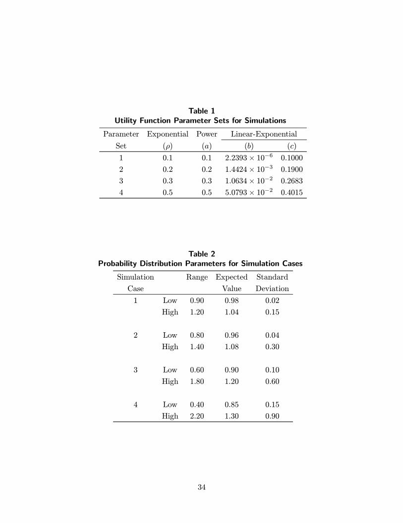
Table 1Utility Function Parameter Sets for Simulations

Parameter Exponential Power Linear-Exponential

Set (½) (a) (b) (c)

1 0.1 0.1 2.2393£ 10¡6 0.1000

2 0.2 0.2 1.4424£ 10¡3 0.1900

3 0.3 0.3 1.0634£ 10¡2 0.2683

4 0.5 0.5 5.0793£ 10¡2 0.4015

Table 2Probability Distribution Parameters for Simulation Cases

Simulation Range Expected Standard

Case Value Deviation

1 Low 0.90 0.98 0.02

High 1.20 1.04 0.15

2 Low 0.80 0.96 0.04

High 1.40 1.08 0.30

3 Low 0.60 0.90 0.10

High 1.80 1.20 0.60

4 Low 0.40 0.85 0.15

High 2.20 1.30 0.90

34

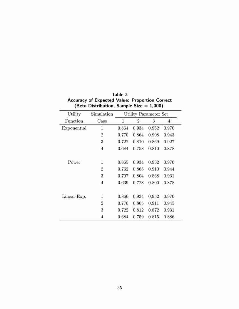
Table 3Accuracy of Expected Value: Proportion Correct

(Beta Distribution, Sample Size = 1,000)

Utility Simulation Utility Parameter Set

Function Case 1 2 3 4

Exponential 1 0.864 0.934 0.952 0.970

2 0.770 0.864 0.908 0.943

3 0.722 0.810 0.869 0.927

4 0.684 0.758 0.810 0.878

Power 1 0.865 0.934 0.952 0.970

2 0.762 0.865 0.910 0.944

3 0.707 0.804 0.868 0.931

4 0.639 0.728 0.800 0.878

Linear-Exp. 1 0.866 0.934 0.952 0.970

2 0.770 0.865 0.911 0.945

3 0.722 0.812 0.872 0.931

4 0.684 0.759 0.815 0.886

35

Table 4Accuracy of Expected Value: Mean CE Loss(Beta Distribution, Sample Size = 1,000)



Exponential 1 0.00581 0.00336 0.00215 0.00135

2 0.02096 0.01163 0.00809 0.00512

3 0.05634 0.03692 0.02691 0.01804

4 0.09590 0.07367 0.05538 0.03551

Power 1 0.00584 0.00328 0.00208 0.00130

2 0.02150 0.01171 0.00802 0.00493

3 0.06636 0.04139 0.02825 0.01834

4 0.11737 0.09465 0.06938 0.03944

Linear-Exp. 1 0.00584 0.00332 0.00211 0.00132

2 0.02082 0.01155 0.00813 0.00508

3 0.05627 0.03710 0.02650 0.01761

4 0.09600 0.07529 0.05646 0.03499

36

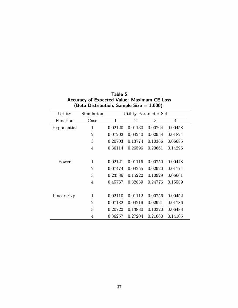
Table 5Accuracy of Expected Value: Maximum CE Loss




Exponential 1 0.02120 0.01130 0.00764 0.00458

2 0.07202 0.04240 0.02958 0.01824

3 0.20703 0.13774 0.10366 0.06685

4 0.36114 0.26596 0.20661 0.14296

Power 1 0.02121 0.01116 0.00750 0.00448

2 0.07474 0.04255 0.02920 0.01774

3 0.23586 0.15222 0.10929 0.06661

4 0.45757 0.32839 0.24776 0.15589

Linear-Exp. 1 0.02110 0.01112 0.00756 0.00452

2 0.07182 0.04219 0.02921 0.01786

3 0.20722 0.13880 0.10320 0.06488

4 0.36257 0.27204 0.21060 0.14105

37

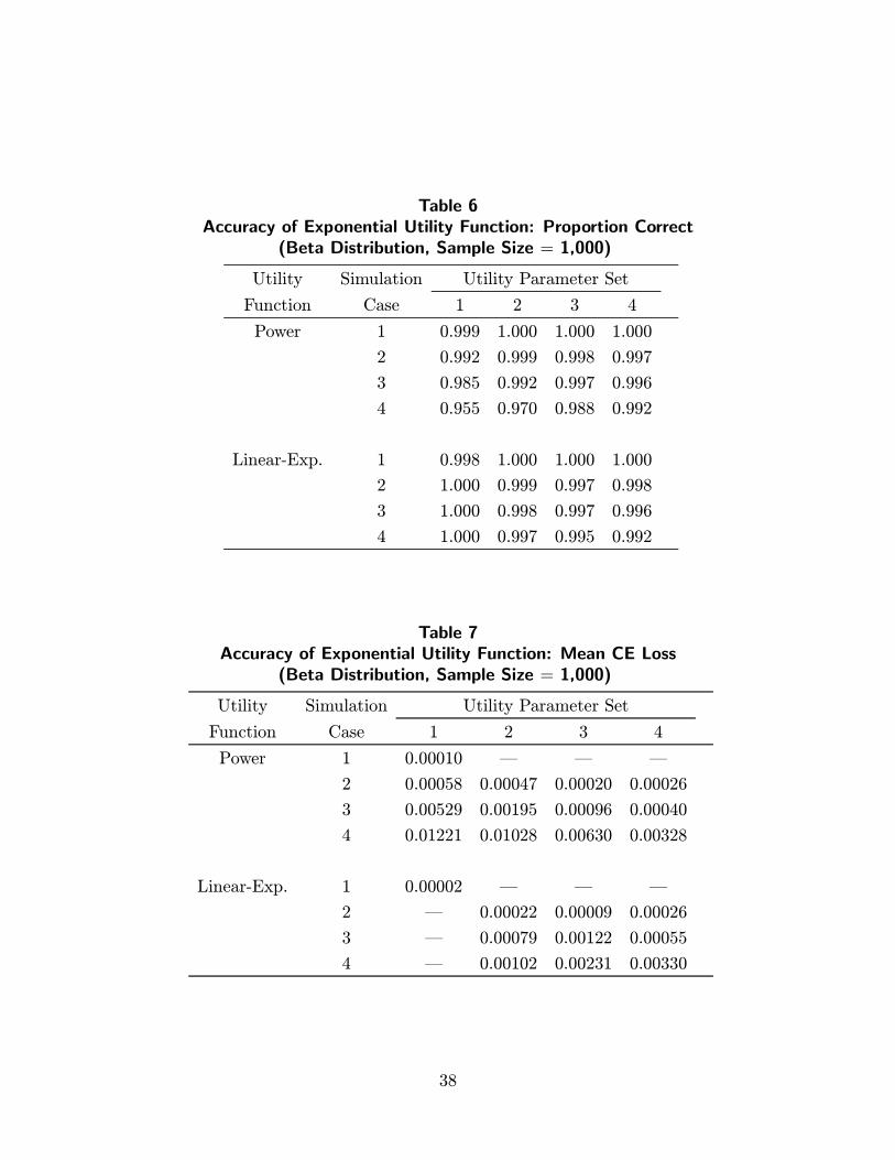
Table 6Accuracy of Exponential Utility Function: Proportion Correct




Power 1 0.999 1.000 1.000 1.000

2 0.992 0.999 0.998 0.997

3 0.985 0.992 0.997 0.996

4 0.955 0.970 0.988 0.992

Linear-Exp. 1 0.998 1.000 1.000 1.000

2 1.000 0.999 0.997 0.998

3 1.000 0.998 0.997 0.996

4 1.000 0.997 0.995 0.992

Table 7Accuracy of Exponential Utility Function: Mean CE Loss




Power 1 0.00010 | | |

2 0.00058 0.00047 0.00020 0.00026

3 0.00529 0.00195 0.00096 0.00040

4 0.01221 0.01028 0.00630 0.00328

Linear-Exp. 1 0.00002 | | |

2 | 0.00022 0.00009 0.00026

3 | 0.00079 0.00122 0.00055

4 | 0.00102 0.00231 0.00330

38

Table 8Accuracy of Exponential Utility Function: Maximum CE Loss




Power 1 0.00010 | | |

2 0.00111 0.00047 0.00024 0.00049

3 0.01588 0.00588 0.00239 0.00078

4 0.04960 0.03314 0.02095 0.00603

Linear-Exp. 1 0.00002 | | |

2 | 0.00022 0.00014 0.00036

3 | 0.00119 0.00223 0.00146

4 | 0.00140 0.00550 0.00734

Table 9Accuracy of Exponential Utility Function

(Beta Distribution, Linear-Exponential Utility Function, Sample Size = 1,000)

Utility Simulation Proportion CE Loss for Errors

Function Case Correct Mean Maximum

\3" 1 1.000 | |

2 0.999 0.00003 0.00003

3 1.000 | |

4 0.999 0.00018 0.00018

\10" 1 0.987 0.00072 0.00139

2 0.987 0.00105 0.00277

3 0.992 0.00313 0.00795

4 0.992 0.00162 0.00357

39

Table 10Accuracy of Expected Value

(P = 0:75, Utility Parameter Set 1)



Exponential 1 0.652 0.03772 0.12474

2 0.605 0.11374 0.35874

3 0.588 0.25477 0.75287

4 0.561 0.25541 0.83636

Power 1 0.648 0.04183 0.14113

2 0.600 0.13078 0.41966

3 0.588 0.29766 0.86914

4 0.560 0.29753 0.97060

Linear-Exp. 1 0.653 0.03772 0.12460

2 0.605 0.11373 0.35877

3 0.588 0.25487 0.75350

4 0.561 0.25554 0.83778


(P = 0:75, Utility Parameter Set 1)



Power 1 0.996 0.00095 0.00140

2 0.995 0.00113 0.00236

3 1.000 | |

4 0.999 0.00014 0.00014

Linear-Exp. 1 0.999 0.00003 0.00003

2 1.000 | |

3 1.000 | |

4 1.000 | |

40

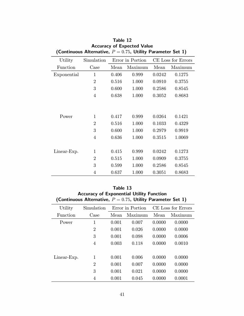
Table 12Accuracy of Expected Value

(Continuous Alternative, P = 0:75, Utility Parameter Set 1)

Utility Simulation Error in Portion CE Loss for Errors

Function Case Mean Maximum Mean Maximum

Exponential 1 0.406 0.999 0.0242 0.1275

2 0.516 1.000 0.0910 0.3755

3 0.600 1.000 0.2586 0.8545

4 0.638 1.000 0.3052 0.8683

Power 1 0.417 0.999 0.0264 0.1421

2 0.516 1.000 0.1033 0.4329

3 0.600 1.000 0.2979 0.9919

4 0.636 1.000 0.3515 1.0069

Linear-Exp. 1 0.415 0.999 0.0242 0.1273

2 0.515 1.000 0.0909 0.3755

3 0.599 1.000 0.2586 0.8545

4 0.637 1.000 0.3051 0.8683


(Continuous Alternative, P = 0:75, Utility Parameter Set 1)

Utility Simulation Error in Portion CE Loss for Errors

Function Case Mean Maximum Mean Maximum

Power 1 0.001 0.007 0.0000 0.0000

2 0.001 0.026 0.0000 0.0000

3 0.001 0.098 0.0000 0.0006

4 0.003 0.118 0.0000 0.0010

Linear-Exp. 1 0.001 0.006 0.0000 0.0000

2 0.001 0.007 0.0000 0.0000

3 0.001 0.021 0.0000 0.0000

4 0.001 0.045 0.0000 0.0001

41

approximating risk aversion in decision analysis...

Documents