Approximation and Geometry of the Reach

Eddie Aamari

Inria Saclay, Université d’Orsay

Gudhi/TopData Workshop 2016, Porquerolles

10/20/2016

With J. Kim, F. Chazal, B. Michel, A. Rinaldo, L. Wasserman

1 / 31

RegularityRegularity and scale parameters are crucial in approximationsproblems, and in actual implementation for estimation.

Classical regularity classes: Hölder, Sobolev, Besov, ...?Such classes allow to control variations in the form of increments

‖f (x)− f (y)‖ ≤ K ‖x − y‖α .

→ Drives the difficulty of the statistical problem.

2 / 31

Regularity Without Coordinates?Without natural coordinates, usual increments ” ‖f (x)− f (y)‖ ” nolonger make sense.Need for an intrinsic way to describe the difficulty of a problem.

Some computational geometers and statisticians use the reach.

3 / 31

Bibliography

First introduced by H. Federer (1957), the reach is a regularity andscale parameter that has recently grown popular in the geometricinference literature.• Homology Inference: Niyogi, Smale, Weinberger, Dey, Lieutier• Manifold Reconstruction: Boissonnat, Ghosh, CMU TopStatgroup

• Volume Estimation: Cuevas, Fraiman, Pateiro-López,Rodríguez-Casal

• Manifold Clustering: Arias-Castro, Lerman, Zhang

4 / 31

Medial AxisThe medial axis of M ⊂ RD is the set of points that have at leasttwo nearest neighbors on M .

Med(M ) = {z ∈ RD, z has several nearest neighbors on M},

Figure : Voronoi diagram of a point cloud

5 / 31

Medial AxisThe medial axis of M ⊂ RD is the set of points that have at leasttwo nearest neighbors on M .

Med(M ) = {z ∈ RD, z has several nearest neighbors on M},

M

Med(M)

Figure : Medial axis of a continuous subset

6 / 31

ReachFor a closed subset M ⊂ RD, the reach τM of M is the least distanceto its medial axis.

τM = infx∈M

d (x,med(M )) ,

where d(x,A) = infa∈A‖x − a‖ for all x ∈ RD.

τM

M

Med(M)

One can also flip the formula, in the sense that

τM = infz∈Med(M)

d (z,M ) .

7 / 31

Global Regularity

τM

τM

Figure : The smaller τM , the tighter a bottleneck structure is possible.

8 / 31

Local Regularity

M

Med(M)

τM

Figure : High curvature ≡ Small radius of curvature ≡ τM → 0.

Proposition (Nyiogi, Smale, Weinberger — 2006)Let II denote the second fundamental form of M. For all unit tangentvector v ∈ TxM, IIx(v, v) ≤ 1/τM .

Proposition (Dey, Li — 2009)The sectional curvatures κ satisfy |κ| ≤ 2/τ2

M .

9 / 31

Theorem (A,K,C,M,R,W — 2016?)For a closed C3 submanifold M ⊂ RD, the reach can be attained with:

q1

q2

B(z0, τM )

Med(M)

M

||q1 − q2|| = 2τM

z0

- A bottleneck.

q0

z0

τM

M

Med(M)

B(z0, τM )

- No reach attaining pair.

q1 q2

z0τM

M

Med(M)

B(z0, τM )

||q1 − q2|| < 2τM

- A reach attaining pair,- No bottleneck.

10 / 31

Global and Local Reach

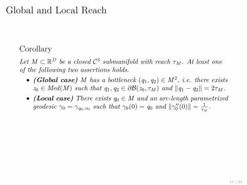
CorollaryLet M ⊂ RD be a closed C3 submanifold with reach τM . At least oneof the following two assertions holds.• (Global case) M has a bottleneck (q1, q2) ∈ M 2, i.e. there existsz0 ∈ Med(M ) such that q1, q2 ∈ ∂B(z0, τM ) and ‖q1 − q2‖ = 2τM .

• (Local case) There exists q0 ∈ M and an arc-length parametrizedgeodesic γ0 = γq0,v0 such that γ0(0) = q0 and ‖γ′′0 (0)‖ = 1

τM.

In view of estimation: we do not know a priori which case theunderlying M belongs to.→ An estimator should handle both cases indiscriminately.

11 / 31

Global and Local Reach

CorollaryLet M ⊂ RD be a closed C3 submanifold with reach τM . At least oneof the following two assertions holds.• (Global case) M has a bottleneck (q1, q2) ∈ M 2, i.e. there existsz0 ∈ Med(M ) such that q1, q2 ∈ ∂B(z0, τM ) and ‖q1 − q2‖ = 2τM .

• (Local case) There exists q0 ∈ M and an arc-length parametrizedgeodesic γ0 = γq0,v0 such that γ0(0) = q0 and ‖γ′′0 (0)‖ = 1

τM.

In view of estimation: we do not know a priori which case theunderlying M belongs to.→ An estimator should handle both cases indiscriminately.

12 / 31

Geometric and Statistical Model

Definition (Geometric Model)We letMd,D

τmin ,L denote the set of connected compact submanifoldsM ⊂ RD without boundary, such that τM ≥ τmin > 0, and for whichevery arc-length parametrized geodesic γp,v is C3 and satisfies∥∥γ′′′p,v(0)

∥∥ ≤ L.

Definition (Statistical Model)We let Qd,D

τmin ,L,fmindenote the set of distributions Q having support

M ∈Md,Dτmin ,L and with a density f = dQ

dvolM ≥ fmin > 0 on M.

From now on, we assume that the tangent spaces are known atobserved points. Data takes the form (X1,TX1M ), . . . , (Xn,TXnM ).

In these models, estimating τM is equivalent to estimate 1/τM .13 / 31

A (Crucial) Local Formulation

Proposition (Federer — 1957)For all closed submanifold M ⊂ RD,

τM = infp 6=q∈M

‖q − p‖2

2d (q − p,TpM ) .

M

TpM

d (q − p, TpM)‖q − p‖‖q−p‖2

2d(q−p,TpM)

q

p

14 / 31

A (Crucial) Local Formulation

Proposition (Federer — 1957)For all closed submanifold M ⊂ RD,

τM = infp 6=q∈M

‖q − p‖2

2d (q − p,TpM ) .

Plugin Estimator: Let X = {x1, . . . , xn} ⊂ M be a finite pointcloud. Define

τ̂ (X) = infxi 6=xj∈X

‖xj − xi‖2

2d(xj − xi ,TxiM ) .

M

TpM

d (q − p, TpM)‖q − p‖‖q−p‖2

2d(q−p,TpM)

q

p 15 / 31

A (Crucial) Local Formulation

Proposition (Federer — 1957)For all closed submanifold M ⊂ RD,

τM = infp 6=q∈M

‖q − p‖2

2d (q − p,TpM ) .

Plugin Estimator: Let X = {x1, . . . , xn} ⊂ M be a finite pointcloud. Define

τ̂ (X) = infxi 6=xj∈X

‖xj − xi‖2

2d(xj − xi ,TxiM ) .

τ̂ is decreasing for inclusion: if Y ⊂ X ⊂ M ,τ̂(Y) ≥ τ̂(X) ≥ τ̂(M ) = τM .

16 / 31

Global Case

Proposition (A,K,C,M,R,W — 2016?)Let M ⊂ RD be a submanifold with reach τM that has a bottleneckq1, q2 ∈ M. Let X ⊂ M.If there exist x, y ∈ X with ‖q1 − x‖ < τM and ‖q2 − y‖ < τM ,

1τM≥ 1τ̂(X) ≥

1τ̂({x, y}) ≥

1τM− 9

2τ2M

max {dM (q1, x), dM (q2, y)} .

q1

M

y

τMτ̂(x, y)

TxMx

q2

17 / 31

Minimax Estimate in the Global Case

If Xn = {X1, . . . ,Xn} is a i.i.d. sample, the integrated bound followsby lower bounding the probability to get two points Xi and Xj closeto q1 and q2.

CorollaryLet P ∈ Pd,D

τmin,L,fminand M = supp(P). Assume M has a bottleneck

q1, q2 ∈ M. Then,

EPn

[∣∣∣∣ 1τ̂(Xn) −

1τM

∣∣∣∣p]≤ Cp,d,τmin ,L,fminn−

pd ,

where Cp,d,τmin,L,fmin depends only on p, d, τmin,L and fmin.

18 / 31

Local CaseAssume there exist q0 ∈ M and v0 ∈ Tq0M with

∥∥γ′′q0,v0(0)

∥∥ = 1/τM .

q0

v0

q1

v1

θ

Mγ0

γ1

• (Principal Curvature Stability). If dM (q0, q1) and θ = ∠(v0, v1)are small, ∥∥γ′′q1,v1

(0)∥∥ ' ∥∥γ′′q0,v0

(0)∥∥ = 1/τM .

• (Directional Curvature Estimation). Write γx→y for the geodesicjoining x to y. If ‖y − x‖ is small,

‖y − x‖2

2d (y − x,TxM ) '∥∥γ′′x→y(0)

∥∥ .

19 / 31

Local CaseAssume there exist q0 ∈ M and v0 ∈ Tq0M with

∥∥γ′′q0,v0(0)

∥∥ = 1/τM .

q0

v0

θ

Mγ0

γx→yxy

TxM

• (Principal Curvature Stability). If dM (q0, q1) and θ = ∠(v0, v1)are small, ∥∥γ′′q1,v1

(0)∥∥ ' ∥∥γ′′q0,v0

(0)∥∥ = 1/τM .

• (Directional Curvature Estimation). Write γx→y for the geodesicjoining x to y. If ‖y − x‖ is small,

‖y − x‖2

2d (y − x,TxM ) '∥∥γ′′x→y(0)

∥∥ .20 / 31

Local Case

Proposition (A,K,C,M,R,W — 2016?)Let M ∈Md,D

τmin,L be such that there exist q0 ∈ M and a geodesic γ0

with γ0(0) = q0 and ‖γ′′0 (0)‖ = 1τM

.Let X ⊂ M and x, y ∈ X be such that x, y ∈ BM

(q0,

τM4

). Let γx→y be

the geodesic joining x and y and θ = ∠(γ′0(0), γ′x→y(0)

).

1τM≥ 1τ̂(X) ≥

1τ̂({x, y}) ≥

1τM−

{4 sin2 θ

τM+ 37dM (x, y)2

τ3M

+(

8τ3

M+ L

)dM (x, y) + 2

3LdM (q0, x)}.

q0

v0

θ

Mγ0

γx→yxy

TxM

21 / 31

Minimax Estimate in the Local Case

If Xn = {X1, . . . ,Xn} is a i.i.d. sample, the integrated bound followsby lower bounding the probability to get two points Xi ,Xj close to q0and almost aligned with v0.

Corollary (A,K,C,M,R,W — 2016?)Let P ∈ Pd,D

τmin,L,fminand M = supp(P). Suppose there exists q0 ∈ M

and a geodesic γ0 such that γ0(0) = q0 and ‖γ′′0 (0)‖ = 1τM

. Then,

EPn

[∣∣∣∣ 1τ̂(Xn) −

1τM

∣∣∣∣p]≤ Cτmin,L,fminn−

4p5d−1 ,

where Cτmin,L,fmin depends only on τmin, L and fmin.

22 / 31

Minimax Risk

Let us denote by Rn the minimax risk over Pd,Dτmin ,L,fmin

.

Rpn = inf

τ̂nsup

P∈Pd,Dτmin ,L,fmin

EPn

∣∣∣∣ 1τP− 1τ̂n

∣∣∣∣p,

where the infimum is taken over all the estimators τ̂n computed overan n-sample (X1,TX1), . . . , (Xn,TXn ).

23 / 31

Minimax Risk

Let us denote by Rn the minimax risk over Pd,Dτmin ,L,fmin

.

Rpn = inf

τ̂nsup

P∈Pd,Dτmin ,L,fmin

EPn

∣∣∣∣ 1τP− 1τ̂n

∣∣∣∣p,

where the infimum is taken over all the estimators τ̂n computed overan n-sample (X1,TX1), . . . , (Xn,TXn ).

CorollaryFor n large enough,

Rpn ≤ Cp,τmin,L,fminn−

4p5d−1 ,

for some constant Cp,τmin,L,fmin depending only on p, τmin,L and fmin.

24 / 31

Minimax Risk

Let us denote by Rn the minimax risk over Pd,Dτmin ,L,fmin

.

Rpn = inf

τ̂nsup

P∈Pd,Dτmin ,L,fmin

EPn

∣∣∣∣ 1τP− 1τ̂n

∣∣∣∣p,

where the infimum is taken over all the estimators τ̂n computed overan n-sample (X1,TX1), . . . , (Xn,TXn ).

Proposition (A,K,C,M,R,W — 2016?)Assume that (4π)dτd

min ≤ f−1min/2, L ≥ 1

2τ2min

and D ≥ 2d. Then,

cp,τminn−p/d ≤ Rpn ≤ Cp,τmin,L,fminn−

4p5d−1 ,

for n large enough.

25 / 31

Le Cam’s Lemma

For two probability distributions Q,Q′ on RD, the total variationdistance between them is

TV (Q,Q′) = supB∈B(RD)

|Q(B)−Q′(B)| .

Theorem (L. Le Cam)Let Q,Q′ ∈ Qd,D

τmin ,L,fminwith respective supports M and M ′.

Then for all n ≥ 1,

Rpn ≥ cp

∣∣∣∣ 1τM− 1τM ′

∣∣∣∣p(1− TV (Q,Q′))2n

.

Deriving a minimax lower bound amounts to find Q,Q′ such that:•

∣∣∣ 1τM− 1

τM′

∣∣∣ is large,• TV (Q,Q′) is small.

26 / 31

Le Cam’s Lemma Heuristic

For η ≈ `3 and `d ≈ 1/n,

•∣∣∣ 1τM− 1

τM′

∣∣∣ & ( 1n

)1/d ,

• with high probability, a n-sample does not separate M and M ′.

η

2τmin

`

M ′

OM

27 / 31

What if Tangent Spaces are Unknown?

Given a point cloud X ⊂ RD and a family T = {Tx}x∈X of linearsubspaces of RD indexed by X, the plug-in estimator is defined as

τ̂(X,T ) = infx 6=y∈X

‖y − x‖2

2d(y − x,Tx) .

This generalises the previous estimator τ̂(X) = τ̂(X,TM ). Noticethat,

τM = infx 6=y∈M

‖y − x‖2

2d(y − x,TxM ) = τ̂(M ,TM ).

28 / 31

Tangent Space StabilityFor two linear subspaces U ,V ∈ Gd,D, let ∠(U ,V ) = ‖πU − πV‖opdenote their principal angle.

PropositionLet X be a subset of RD and T = {Tx}x∈X, T̃ = {T̃x}x∈X be twofamilies of linear subspaces of RD indexed by X.Assume X to be δ-sparse, T and T̃ to be θ-close, in the sense that

infx 6=y∈X

‖y − x‖ ≥ δ and supx∈X

∠(Tx , T̃x) ≤ θ.

Then, ∣∣∣∣ 1τ̂(X,T ) −

1τ̂(X, T̃ )

∣∣∣∣ ≤ 2θδ.

CorollaryAll the previous deterministic upper bounds hold for τ̂

(X, T̃

)with an

extra error term 2θ/δ.29 / 31

Yet to Be Done

• Finish to write the paper...• Make the minimax upper and lower bounds match.• Include noise. For this, it could boil down to prove that themodelMd,D

τmin ,L is stable under the action of C3-diffeomorphisms.• Give minimax upper bounds with unknown tangent spaces.• Tackle related regularity parameters such as λ-reach, µ-reach orlocal feature size.

Thanks

30 / 31

Yet to Be Done

• Finish to write the paper...• Make the minimax upper and lower bounds match.• Include noise. For this, it could boil down to prove that themodelMd,D

τmin ,L is stable under the action of C3-diffeomorphisms.• Give minimax upper bounds with unknown tangent spaces.• Tackle related regularity parameters such as λ-reach, µ-reach orlocal feature size.

Thanks

31 / 31