approximation chap

8/12/2019 Approximation Chap

http://slidepdf.com/reader/full/approximation-chap 1/31

D. Levy

4 Approximations

4.1 Background

In this chapter we are interested in approximation problems. Generally speaking, start-ing from a function f (x) we would like to find a different function g(x) that belongsto a given class of functions and is “close” to f (x) in some sense. As far as the classof functions that g(x) belongs to, we will typically assume that g(x) is a polynomialof a given degree (though it can be a trigonometric function, or any other function).A typical approximation problem, will therefore be: find the “closest” polynomial of degree n to f (x).

What do we mean by “close”? There are different ways of measuring the “distance”between two functions. We will focus on two such measurements (among many): the L∞-norm and the L2-norm. We chose to focus on these two examples because of the differentmathematical techniques that are required to solve the corresponding approximationproblems.

We start with several definitions. We recall that a norm on a vector space V overR is a function · : V → R with the following properties:

1. λf = |λ|f , ∀λ ∈ R and ∀f ∈ V .

2. f 0, ∀f ∈ V . Also f = 0 iff f is the zero element of V .

3. The triangle inequality: f + g f + g, ∀f, g ∈ V .

We assume that the function f (x)

∈ C 0[a, b] (continuous on [a, b]). A continuous

function on a closed interval obtains a maximum in the interval. We can therefore definethe L∞ norm (also known as the maximum norm) of such a function by

f ∞ = maxaxb

|f (x)|. (4.1)

The L∞-distance between two functions f (x), g(x) ∈ C 0[a, b] is thus given by

f − g∞ = maxaxb

|f (x) − g(x)|. (4.2)

We note that the definition of the L∞-norm can be extended to functions that are less

regular than continuous functions. This generalization requires some subtleties thatwe would like to avoid in the following discussion, hence, we will limit ourselves tocontinuous functions.

We proceed by defining the L2-norm of a continuous function f (x) as

f 2 =

ba

|f (x)|2dx. (4.3)

1



4.1 Background D. Levy

The L2 function space is the collection of functions f (x) for which f 2 < ∞. Of course, we do not have to assume that f (x) is continuous for the definition (4.3) tomake sense. However, if we allow f (x) to be discontinuous, we then have to be morerigorous in terms of the definition of the interval so that we end up with a norm (the

problem is, e.g., in defining what is the “zero” element in the space). We therefore limitourselves also in this case to continuous functions only. The L2-distance between twofunctions f (x) and g(x) is

f − g2 =

ba

|f (x) − g(x)|2 dx. (4.4)

At this point, a natural question is how important is the choice of norm in terms of the solution of the approximation problem. It is easy to see that the value of the normof a function may vary substantially based on the function as well as the choice of the

norm. For example, assume that f ∞ < ∞. Then, clearly

f 2 =

ba

|f |2dx ≤ (b − a)f ∞.

On the other hand, it is easy to construct a function with an arbitrary small f 2 andan arbitrarily large f ∞. Hence, the choice of norm may have a significant impact onthe solution of the approximation problem.

As you have probably already anticipated, there is a strong connection between someapproximation problems and interpolation problems. For example, one possible method

of constructing an approximation to a given function is by sampling it at certain pointsand then interpolating the sampled data. Is that the best we can do? Sometimes theanswer is positive, but the problem still remains difficult because we have to determinethe best sampling points. We will address these issues in the following sections.

The following theorem, the Weierstrass approximation theorem, plays a central rolein any discussion of approximations of functions. Loosely speaking, this theorem statesthat any continuous function can be approached as close as we want to with polynomials,assuming that the polynomials can be of any degree. We formulate this theorem in theL∞ norm and note that a similar theorem holds also in the L2 sense. We let Πn denotethe space of polynomials of degree n.

Theorem 4.1 (Weierstrass Approximation Theorem) Let f (x) be a continuous

function on [a, b]. Then there exists a sequence of polynomials P n(x) that converges

uniformly to f (x) on [a, b], i.e., ∀ε > 0, there exists an N ∈ N and polynomials P n(x) ∈Πn, such that ∀x ∈ [a, b]

|f (x) − P n(x)| < ε, ∀n N.

2



D. Levy 4.1 Background

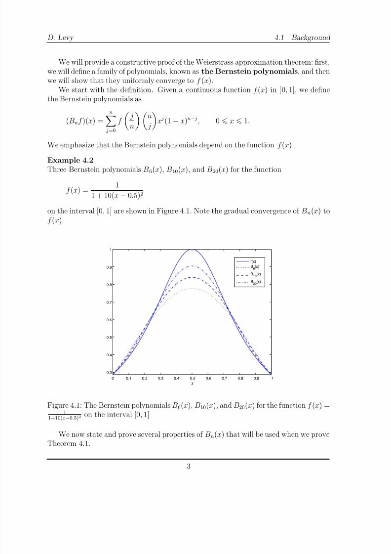
We will provide a constructive proof of the Weierstrass approximation theorem: first,we will define a family of polynomials, known as the Bernstein polynomials, and thenwe will show that they uniformly converge to f (x).

We start with the definition. Given a continuous function f (x) in [0, 1], we define

the Bernstein polynomials as

(Bnf )(x) =n

j=0

f

j

n

n

j

x j(1 − x)n− j, 0 x 1.

We emphasize that the Bernstein polynomials depend on the function f (x).

Example 4.2Three Bernstein polynomials B6(x), B10(x), and B20(x) for the function

f (x) =

1

1 + 10(x − 0.5)2

on the interval [0, 1] are shown in Figure 4.1. Note the gradual convergence of Bn(x) tof (x).

0 0.1 0.2 0.3 0.4 0.5 0.6 0.7 0.8 0.9 1

0.3

0.4

0.5

0.6

0.7

0.8

0.9

1

x

f(x)

B6

(x)

B10

(x)

B20

(x)

Figure 4.1: The Bernstein polynomials B6(x), B10(x), and B20(x) for the function f (x) =1

1+10(x−0.5)2 on the interval [0, 1]

We now state and prove several properties of Bn(x) that will be used when we proveTheorem 4.1.

3



4.1 Background D. Levy

Lemma 4.3 The following relations hold:

1. (Bn1)(x) = 1

2. (Bnx)(x) = x

3. (Bnx2)(x) = n − 1

n x2 +

x

n.

Proof.

(Bn1)(x) =n

j=0

n

j

x j(1 − x)n− j = (x + (1 − x))n = 1.

(Bnx)(x) =n

j=0

j

nn

jx j(1

−x)n− j = x

n

j=1n − 1

j − 1x j−1(1

−x)n− j

= xn−1 j=0

n − 1

j

x j(1 − x)n−1− j = x[x + (1 − x)]n−1 = x.

Finally, j

n

2n

j

=

j

n

(n − 1)!

(n − j)!( j − 1)! =

n − 1

n − 1

j − 1

n

(n − 1)!

(n − j)!( j − 1)! +

1

n

(n − 1)!

(n − j)!( j − 1)!

= n − 1

n

n − 2

j − 2

+

1

n

n − 1

j − 1

.

Hence

(Bnx2)(x) =n

j=0

j

n

2n

j

x j(1 − x)n− j

= n − 1

n x2

n j=2

n − 2

j − 2

x j−2(1 − x)n− j +

1

nx

n j=1

n − 1

j − 1

x j−1(1 − x)n− j

= n − 1

n x2(x + (1 − x))n−2 +

1

nx(x + (1 − x))n−1 =

n − 1

n x2 +

x

n.

In the following lemma we state several additional properties of the Bernstein poly-nomials. The proof is left as an exercise.

Lemma 4.4 For all functions f (x), g(x) that are continuous in [0, 1], and ∀α ∈ R

1. Linearity.

(Bn(αf + g))(x) = α(Bnf )(x) + (Bng)(x).

4



D. Levy 4.1 Background

2. Monotonicity. If f (x) g(x) ∀x ∈ [0, 1], then

(Bnf )(x) (Bng)(x).

Also, if |f (x)| g(x) ∀x ∈ [0, 1] then

|(Bnf )(x)| (Bng)(x).

3. Positivity. If f (x) 0 then

(Bnf )(x) 0.

We are now ready to prove the Weierstrass approximation theorem, Theorem 4.1.

Proof. We will prove the theorem in the interval [0, 1]. The extension to [a, b] is left as

an exercise. Since f (x) is continuous on a closed interval, it is uniformly continuous.Hence ∀x, y ∈ [0, 1], such that |x − y| δ ,

|f (x) − f (y)| ε. (4.5)

In addition, since f (x) is continuous on a closed interval, it is also bounded. Let

M = maxx∈[0,1]

|f (x)|.

Fix any point a ∈ [0, 1]. If |x − a| δ then (4.5) holds. If |x − a| > δ then

|f (x) − f (a)| 2M 2M x

−a

δ 2

.

(at first sight this seems to be a strange way of upper bounding a function. We willuse it later on to our advantage). Combining the estimates for both cases we have

|f (x) − f (a)| ε + 2M

δ 2 (x − a)2.

We would now like to estimate the difference between Bnf and f . The linearity of Bn

and the property (Bn1)(x) = 1 imply that

Bn(f − f (a))(x) = (Bnf )(x) − f (a).

Hence using the monotonicity of Bn and the mapping properties of x and x2, we have,

|Bnf (x) − f (a)| Bn

ε +

2M

δ 2 (x − a)2

= ε +

2M

δ 2

n − 1

n x2 +

x

n − 2ax + a2

= ε + 2M

δ 2 (x − a)2 +

2M

δ 2x − x2

n .

5



4.2 The Minimax Approximation Problem D. Levy

Evaluating at x = a we have (observing that maxa∈[0,1](a − a2) = 14

)

|Bnf (a) − f (a)| ε + 2M

δ 2a − a2

n ε +

M

2δ 2n. (4.6)

The point a was arbitrary so the result (4.6) holds for any point a ∈ [0, 1]. ChoosingN M

2δ2ε we have ∀n N ,

Bnf − f ∞ ε + M

2δ 2N 2ε.

• Is interpolation a good way of approximating functions in the ∞-norm? Notnecessarily. Discuss Runge’s example...

4.2 The Minimax Approximation Problem

We assume that the function f (x) is continuous on [a, b], and assume that P n(x) is apolynomial of degree n. We recall that the L∞-distance between f (x) and P n(x) onthe interval [a, b] is given by

f − P n∞ = maxaxb

|f (x) − P n(x)|. (4.7)

Clearly, we can construct polynomials that will have an arbitrary large distance fromf (x). The question we would like to address is how close can we get to f (x) (in the L∞

sense) with polynomials of a given degree. We define dn(f ) as the infimum of (4.7) overall polynomials of degree n, i.e.,

dn(f ) = inf P n∈Πn

f − P n∞ (4.8)

The goal is to find a polynomial P ∗n(x) for which the infimum (4.8) is actually ob-tained, i.e.,

dn(f ) = f − P ∗n(x)∞. (4.9)

We will refer to a polynomial P ∗n(x) that satisfies (4.9) as a polynomial of best

approximation or the minimax polynomial. The minimal distance in (4.9) willbe referred to as the minimax error.

The theory we will explore in the following sections will show that the minimaxpolynomial always exists and is unique. We will also provide a characterization of the minimax polynomial that will allow us to identify it if we actually see it. Thegeneral construction of the minimax polynomial will not be addressed in this text as itis relatively technically involved. We will limit ourselves to simple examples.

6



D. Levy 4.2 The Minimax Approximation Problem

Example 4.5We let f (x) be a monotonically increasing and continuous function on the interval [ a, b]and are interested in finding the minimax polynomial of degree zero to f (x) in thatinterval. We denote this minimax polynomial by

P ∗0 (x) ≡ c.

Clearly, the smallest distance between f (x) and P ∗0 in the L∞-norm will be obtained if

c = f (a) + f (b)

2 .

The maximal distance between f (x) and P ∗0 will be attained at both edges and will beequal to

±f (b)

−f (a)

2 .

4.2.1 Existence of the minimax polynomial

The existence of the minimax polynomial is provided by the following theorem.

Theorem 4.6 (Existence) Let f ∈ C 0[a, b]. Then for any n ∈N there exists P ∗n(x) ∈Πn, that minimizes f (x) − P n(x)∞ among all polynomials P (x) ∈ Πn.

Proof. We follow the proof as given in [?]. Let η = (η0, . . . , ηn) be an arbitrary point inRn+1 and let

P n(x) =ni=0

ηixi ∈ Πn.

We also let

φ(η) = φ(η0, . . . , ηn) = f − P n∞.

Our goal is to show that φ obtains a minimum in Rn+1, i.e., that there exists a pointη∗ = (η∗0, . . . , η∗n) such that

φ(η∗) = minη∈Rn+1

φ(η).

Step 1. We first show that φ(η) is a continuous function on Rn+1. For an arbitraryδ = (δ 0, . . . , δ n) ∈ R

n+1, define

q n(x) =ni=0

δ ixi.

7




Then

φ(η + δ ) = f − (P n + q n)∞ ≤ f − P n∞ + q n∞ = φ(η) + q n∞.

Hence

φ(η + δ ) − φ(η) ≤ q n∞ ≤ maxx∈[a,b]

(|δ 0| + |δ 1||x| + . . . + |δ n||x|n).

For any ε > 0, let δ = ε/(1 + c + . . . + cn), where c = max(|a|, |b|). Then for anyδ = (δ 0, . . . , δ n) such that max |δ i| δ , 0 i n,

φ(η + δ ) − φ(η) ε. (4.10)

Similarly

φ(η) = f −P n∞ = f −(P n+q n)+q n∞ f −(P n+q n)∞+q n∞ = φ(η+δ )+q n∞,

which implies that under the same conditions as in (4.10) we also get

φ(η) − φ(η + δ ) ε,

Altogether,

|φ(η + δ ) − φ(η)| ε,

which means that φ is continuous at η. Since η was an arbitrary point in Rn+1, φ iscontinuous in the entire Rn+1.

Step 2. We now construct a compact set in Rn+1 on which φ obtains a minimum. Welet

S =

η ∈ Rn+1 φ(η) ≤ f ∞

.

We have

φ(0) =

f ∞,

hence, 0 ∈ S , and the set S is nonempty. We also note that the set S is bounded andclosed (check!). Since φ is continuous on the entire Rn+1, it is also continuous on S ,and hence it must obtain a minimum on S , say at η∗ ∈ R

n+1, i.e.,

minη∈S

φ(η) = φ(η∗).

8




Step 3. Since 0 ∈ S , we know that

minη∈S

φ(η) φ(0) = f ∞.

Hence, if η ∈

Rn+1 but η

∈ S then

φ(η) > f ∞ minη∈S

φ(η).

This means that the minimum of φ over S is the same as the minimum over the entireRn+1. Therefore

P ∗n(x) =ni=0

η∗i xi, (4.11)

is the best approximation of f (x) in the L∞ norm on [a, b], i.e., it is the minimaxpolynomial, and hence the minimax polynomial exists.

We note that the proof of Theorem 4.6 is not a constructive proof. The proof does

not tell us what the point η∗ is, and hence, we do not know the coefficients of theminimax polynomial as written in (4.11). We will discuss the characterization of theminimax polynomial and some simple cases of its construction in the following sections.

4.2.2 Bounds on the minimax error

It is trivial to obtain an upper bound on the minimax error, since by the definition of dn(f ) in (4.8) we have

dn(f ) f − P n∞, ∀P n(x) ∈ Πn.

A lower bound is provided by the following theorem.

Theorem 4.7 (de la Vallee-Poussin) Let a x0 < x1 < · · · < xn+1 b. Let P n(x)be a polynomial of degree n. Suppose that

f (x j) − P n(x j) = (−1) je j , j = 0, . . . , n + 1,

where all e j = 0 and are of an identical sign. Then

min j

|e j| dn(f ).

Proof. By contradiction. Assume for some Qn(x) that

f − Qn∞ < min j

|e j |.

Then the polynomial

(Qn − P n)(x) = (f − P n)(x) − (f − Qn)(x),

is a polynomial of degree n that has the same sign at x j as does f (x) − P n(x). Thisimplies that (Qn − P n)(x) changes sign at least n + 2 times, and hence it has at leastn + 1 zeros. Being a polynomial of degree n this is possible only if it is identicallyzero, i.e., if P n(x) ≡ Qn(x), which contradicts the assumptions on Qn(x) and P n(x).

9




The triangle inequality implies that

f − 1

2(P ∗n + Qn)∞ ≤ 1

2f − P ∗n∞ +

1

2f − Qn∞ = dn(f ).

Hence, 12

(P ∗n + Qn) ∈ Πn is also a minimax polynomial. The oscillating theorem(Theorem 4.8) implies that there exist x0, . . . , xn+1 ∈ [a, b] such that

|f (xi) − 1

2(P ∗n(xi) + Qn(xi))| = dn(f ), 0 i n + 1. (4.12)

Equation (4.12) can be rewritten as

|f (xi) − P ∗n(xi) + f (xi) − Qn(xi)| = 2dn(f ), 0 i n + 1. (4.13)

Since P ∗n(x) and Qn(x) are both minimax polynomials, we have

|f (xi) − P ∗n(xi)| ≤ f − P ∗n∞ = dn(f ), 0 i n + 1. (4.14)

and

|f (xi) − Qn(xi)| ≤ f − Qn∞ = dn(f ), 0 i n + 1. (4.15)

For any i, equations (4.13)–(4.15) mean that the absolute value of two numbers thatare dn(f ) add up to 2dn(f ). This is possible only if they are equal to each other, i.e.,

f (xi) − P ∗n(xi) = f (xi) − Qn(xi), 0 i n + 1,

i.e.,

(P ∗n − Qn)(xi) = 0, 0 i n + 1.

Hence, the polynomial (P ∗n − Qn)(x) ∈ Πn has n + 2 distinct roots which is possible fora polynomial of degree n only if it is identically zero. Hence

Qn(x) ≡ P ∗n(x),

and the uniqueness of the minimax polynomial is established.

4.2.5 The near-minimax polynomial

We now connect between the minimax approximation problem and polynomial interpo-lation. In order for f (x) − P n(x) to change its sign n + 2 times, there should be n + 1points on which f (x) and P n(x) agree with each other. In other words, we can thinkof P n(x) as a function that interpolates f (x) at (least in) n + 1 points, say x0, . . . , xn.What can we say about these points?

11




We recall that the interpolation error is given by (??),

f (x) − P n(x) = 1

(n + 1)!f (n+1)(ξ )

n

i=0

(x − xi).

If P n(x) is indeed the minimax polynomial, we know that the maximum of

f (n+1)(ξ )ni=0

(x − xi), (4.16)

will oscillate with equal values. Due to the dependency of f (n+1)(ξ ) on the intermediatepoint ξ , we know that minimizing the error term (4.16) is a difficult task. We recall thatinterpolation at the Chebyshev points minimizes the multiplicative part of the errorterm, i.e.,

ni=0

(x − xi).

Hence, choosing x0, . . . , xn to be the Chebyshev points will not result with the minimaxpolynomial, but nevertheless, this relation motivates us to refer to the interpolant atthe Chebyshev points as the near-minimax polynomial. We note that the term “near-minimax” does not mean that the near-minimax polynomial is actually close to theminimax polynomial.

4.2.6 Construction of the minimax polynomial

The characterization of the minimax polynomial in terms of the number of points inwhich the maximum distance should be obtained with oscillating signs allows us toconstruct the minimax polynomial in simple cases by a direct computation.

We are not going to deal with the construction of the minimax polynomial in thegeneral case. The algorithm for doing so is known as the Remez algorithm, and we referthe interested reader to [?] and the references therein.

A simple case where we can demonstrate a direct construction of the polynomial iswhen the function is convex, as done in the following example.

Example 4.10Problem: Let f (x) = ex, x

∈ [1, 3]. Find the minimax polynomial of degree 1, P ∗1 (x).

Solution: Based on the characterization of the minimax polynomial, we will be lookingfor a linear function P ∗1 (x) such that its maximal distance between P ∗1 (x) and f (x) isobtained 3 times with alternative signs. Clearly, in the case of the present problem,since the function is convex, the maximal distance will be obtained at both edges andat one interior point. We will use this observation in the construction that follows.The construction itself is graphically shown in Figure 4.2.

12




1 a 3

x

e1

f (a)

y

l1(a)

e3

←− l2(x)

ex

l1(x)−→

P ∗1 (x)

Figure 4.2: A construction of the linear minimax polynomial for the convex function ex

on [1, 3]

We let l1(x) denote the line that connects the endpoints (1, e) and (3, e3), i.e.,

l1(x) = e + m(x − 1).

Here, the slope m is given by

m = e3 − e

2 . (4.17)

Let l2(x) denote the tangent to f (x) at a point a that is identified such that the slopeis m. Since f (x) = ex, we have ea = m, i.e.,

a = log m.

Now

f (a) = elogm = m,

and

l1(a) = e + m(log m − 1).

Hence, the average between f (a) and l1(a) which we denote by y is given by

y = f (a) + l1(a)

2 =

m + e + m log m − m

2 =

e + m log m

2 .

13



4.3 Least-squares Approximations D. Levy

The minimax polynomial P ∗1 (x) is the line of slope m that passes through (a, y),

P ∗1 (x) − e + m log m

2 = m(x − log m),

i.e.,

P ∗1 (x) = mx + e − m log m

2 ,

where the slope m is given by (4.17). We note that the maximal difference betweenP ∗1 (x) and f (x) is obtained at x = 1, a, 3.

4.3 Least-squares Approximations

4.3.1 The least-squares approximation problem

We recall that the L2-norm of a function f (x) is defined as

f 2 =

ba

|f (x)|2dx.

As before, we let Πn denote the space of all polynomials of degree n. The least-squares approximation problem is to find the polynomial that is the closest to f (x)in the L2-norm among all polynomials of degree n, i.e., to find Q∗

n ∈ Πn such that

f −

Q∗

n

2 = min

Qn∈Πn f −

Qn

2.

4.3.2 Solving the least-squares problem: a direct method

Our goal is to find a polynomial in Πn that minimizes the distance f (x) − Qn(x)2among all polynomials Qn ∈ Πn. We thus consider

Qn(x) =ni=0

aixi.

For convenience, instead of minimizing the L2 norm of the difference, we will minimize

its square. We thus let φ denote the square of the L2-distance between f (x) and Qn(x),i.e.,

φ(a0, . . . , an) =

ba

(f (x) − Qn(x))2dx

=

ba

f 2(x)dx − 2ni=0

ai

ba

xif (x)dx +ni=0

n j=0

aia j

ba

xi+ jdx.

14



D. Levy 4.3 Least-squares Approximations

φ is a function of the n + 1 coefficients in the polynomial Qn(x). This means that wewant to find a point a∗ = (a∗0, . . . , a∗n) ∈ Rn+1 for which φ obtains a minimum. At thispoint

∂φ∂ak

a=a∗

= 0. (4.18)

The condition (4.18) implies that

0 = −2

ba

xkf (x)dx +ni=0

a∗i

ba

xi+kdx +n

j=0

a∗ j

ba

x j+kdx (4.19)

= 2

ni=0

a∗i

ba

xi+kdx − ba

xkf (x)dx

.

This is a linear system for the unknowns (a∗

0, . . . , a∗

n):ni=0

a∗i

ba

xi+kdx =

ba

xkf (x), k = 0, . . . , n . (4.20)

We thus know that the solution of the least-squares problem is the polynomial

Q∗

n(x) =ni=0

a∗i xi,

where the coefficients a∗i , i = 0, . . . , n, are the solution of (4.20), assuming that this

system can be solved. Indeed, the system (4.20) always has a unique solution, whichproves that not only the least-squares problem has a solution, but that it is also unique.

We let H n+1(a, b) denote the (n + 1)× (n + 1) coefficients matrix of the system (4.20)on the interval [a, b], i.e.,

(H n+1(a, b))i,k =

ba

xi+kdx, 0 i, k n.

For example, in the case where [a, b] = [0, 1],

H n(0, 1) =

1/1 1/2 . . . 1/n

1/2 1/3 . . . 1/(n + 1)... ...

1/n 1/(n + 1) . . . 1/(2n − 1)

(4.21)

The matrix (4.21) is known as the Hilbert matrix.

Lemma 4.11 The Hilbert matrix is invertible.

15




Proof. We leave it is an exercise to show that the determinant of H n is given by

det(H n) = (1!2! · · · (n − 1)!)4

1!2! · · · (2n − 1)! .

Hence, det(H n) = 0 and H n is invertible.

Is inverting the Hilbert matrix a good way of solving the least-squares problem? No.There are numerical instabilities that are associated with inverting H . We demonstratethis with the following example.

Example 4.12The Hilbert matrix H 5 is

H 5 =

1/1 1/2 1/3 1/4 1/51/2 1/3 1/4 1/5 1/6

1/3 1/4 1/5 1/6 1/71/4 1/5 1/6 1/7 1/81/5 1/6 1/7 1/8 1/9

The inverse of H 5 is

H 5 =

25 −300 1050 −1400 630−300 4800 −18900 26880 −126001050 −18900 79380 −117600 56700

−1400 26880 −117600 179200 −88200630 −12600 56700 −88200 44100

The condition number of H 5 is 4.77 · 105, which indicates that it is ill-conditioned. Infact, the condition number of H n increases with the dimension n so inverting it becomesmore difficult with an increasing dimension.

4.3.3 Solving the least-squares problem: with orthogonal polynomials

Let {P k}nk=0 be polynomials such that

deg(P k(x)) = k.

Let Qn(x) be a linear combination of the polynomials {P k}nk=0, i.e.,

Qn(x) =n

j=0

c jP j(x). (4.22)

Clearly, Qn(x) is a polynomial of degree n. Define

φ(c0, . . . , cn) =

ba

[f (x) − Qn(x)]2dx.

16




We note that the function φ is a quadratic function of the coefficients of the linearcombination (4.22), {ck}. We would like to minimize φ. Similarly to the calculationsdone in the previous section, at the minimum, c∗ = (c∗0, . . . , c∗n), we have

0 = ∂φ∂ck

c=c∗

= −2 ba

P k(x)f (x)dx + 2n

j=0

c∗ j ba

P j(x)P k(x)dx,

i.e.,

n j=0

c∗ j

ba

P j(x)P k(x)dx =

ba

P k(x)f (x)dx, k = 0, . . . , n . (4.23)

Note the similarity between equation (4.23) and (4.20). There, we used the basis func-tions {xk}nk=0 (a basis of Πn), while here we work with the polynomials {P k(x)}nk=0

instead. The idea now is to choose the polynomials {P k(x)}nk=0 such that the system

(4.23) can be easily solved. This can be done if we choose them in such a way that ba

P i(x)P j(x)dx = δ ij =

1, i = j,0, j = j.

(4.24)

Polynomials that satisfy (4.24) are called orthonormal polynomials. If, indeed, thepolynomials {P k(x)}nk=0 are orthonormal, then (4.23) implies that

c∗ j =

ba

P j(x)f (x)dx, j = 0, . . . , n . (4.25)

The solution of the least-squares problem is a polynomial

Q∗

n(x) =n

j=0

c∗ jP j(x), (4.26)

with coefficients c∗ j , j = 0, . . . , n, that are given by (4.25).

Remark. Polynomials that satisfy

ba

P i(x)P j(x)dx =

ba (P i(x))2, i = j,

0, i = j,

with ba (P i(x))2dx that is not necessarily 1 are called orthogonal polynomials. In

this case, the solution of the least-squares problem is given by the polynomial Q∗

n(x) in(4.26) with the coefficients

c∗ j =

ba

P j(x)f (x)dx ba

(P j(x))2dx, j = 0, . . . , n . (4.27)

17




4.3.4 The weighted least squares problem

A more general least-squares problem is the weighted least squares approximationproblem. We consider a weight function, w(x), to be a continuous on (a, b), non-

negative function with a positive mass, i.e., ba

w(x)dx > 0.

Note that w(x) may be singular at the edges of the interval since we do not requireit to be continuous on the closed interval [a, b]. For any weight w(x), we define thecorresponding weighted L2-norm of a function f (x) as

f 2,w =

ba

(f (x))2w(x)dx.

The weighted least-squares problem is to find the closest polynomial Q∗

n ∈ Πn to f (x),this time in the weighted L2-norm sense, i.e., we look for a polynomial Q∗

n(x) of degree n such that

f − Q∗

n2,w = minQn∈Πn

f − Qn2,w. (4.28)

In order to solve the weighted least-squares problem (4.28) we follow the methodologydescribed in Section 4.3.3, and consider polynomials {P k}nk=0 such that deg(P k(x)) = k.We then consider a polynomial Qn(x) that is written as their linear combination:

Qn(x) =

n j=0

c jP j(x).

By repeating the calculations of Section 4.3.3, we obtain for the coefficients of theminimizer Q∗

n,

n j=0

c∗ j

ba

w(x)P j(x)P k(x)dx =

ba

w(x)P k(x)f (x)dx, k = 0, . . . , n , (4.29)

(compare with (4.23)). The system (4.29) can be easily solved if we choose {P k(x)} tobe orthonormal with respect to the weight w(x), i.e.,

b

a

P i(x)P j(x)w(x)dx = δ ij.

Hence, the solution of the weighted least-squares problem is given by

Q∗

n(x) =n

j=0

c∗ jP j(x), (4.30)

18




where the coefficients are given by

c∗ j =

b

a

P j(x)f (x)w(x)dx, j = 0, . . . , n . (4.31)

Remark. In the case where {P k(x)} are orthogonal but not necessarily normalized,the solution of the weighted least-squares problem is given by

Q∗

n(x) =n

j=0

c∗ jP j(x)

with

c∗ j =

ba

P j(x)f (x)w(x)dx

ba (P j(x))2w(x)dx, j = 0, . . . , n .

4.3.5 Orthogonal polynomials

At this point we already know that orthogonal polynomials play a central role in thesolution of least-squares problems. In this section we will focus on the construction of orthogonal polynomials. The properties of orthogonal polynomials will be studies inSection 4.4.2.

We start by defining the weighted inner product between two functions f (x) andg(x) (with respect to the weight w(x)):

f, gw =

b

a

f (x)g(x)w(x)dx.

To simplify the notations, even in the weighted case, we will typically write f, g insteadof f, gw. Some properties of the weighted inner product include

1. αf,g = f,αg = α f, g , ∀α ∈R.

2. f 1 + f 2, g = f 1, g + f 2, g.

3. f, g = g, f

4. f, f 0 and f, f = 0 iff f ≡ 0. Here we must assume that f (x) is continuousin the interval [a, b]. If it is not continuous, we can have f, f = 0 and f (x) canstill be non-zero (e.g., in one point).

The weighted L2-norm can be obtained from the weighted inner product by

f 2,w =

f, f w.

19




Given a weight w(x), we are interested in constructing orthogonal (or orthonor-mal) polynomials. This can be done using the Gram-Schmidt orthogonalizationprocess, which we now describe in detail.

In the general context of linear algebra, the Gram-Schmidt process is being used to

convert one set of linearly independent vectors to an orthogonal set of vectors that spansthe same subspace as the original set. In our context, we should think about the processas converting one set of polynomials that span the space of polynomials of degree nto an orthogonal set of polynomials that spans the same space Πn. Accordingly, weset the initial set of polynomials as {1, x , x2, . . . , xn}, which we would like to convert toorthogonal polynomials (of an increasing degree) with respect to the weight w(x).

We will first demonstrate the process with the weight w(x) ≡ 1. We will generate aset of orthogonal polynomials {P 0(x), . . . , P n(x)} from {1, x , . . . , xn}. The degree of thepolynomials P i is i.

We start by setting

P 0(x) = 1.

We then let

P 1(x) = x − c01P 0(x) = x − c01.

The orthogonality condition ba P 1P 0dx = 0, implies that b

a

1 · (x − c01)dx = 0,

from which c= (a+b)/2, and thus

P 1(x) = x − a + b2

.

The computation continues in a similar fashion. We set

P 2(x) = x2 − c02P 0(x) − c12(x).

The two unknown coefficients, c02 and c12, are computed from the orthogonality condi-tions. This time, P 2(x) should be orthogonal to P 0(x) and to P 1(x), i.e., b

a

P 2(x)P 0(x)dx = 0, and

ba

P 2(x)P 1(x)dx = 0,

and so on. If, in addition to the orthogonality condition, we would like the polynomialsto be orthonormal, all that remains is to normalize:

P n(x) = P n(x)

P n(x) = P n(x) ba

(P n(x))2dx, ∀n.

The orthogonalization process is identical to the process that we described even whenthe weight w(x) is not uniformly one. In this case, every integral will contain the weight.

20



D. Levy 4.4 Examples of orthogonal polynomials

4.4 Examples of orthogonal polynomials

This section includes several examples of orthogonal polynomials and a very brief sum-mary of some of their properties.

1. Legendre polynomials. We start with the Legendre polynomials. This is afamily of polynomials that are orthogonal with respect to the weight

w(x) ≡ 1,

on the interval [−1, 1].

In addition to deriving the Legendre polynomials through the Gram-Schmidt or-thogonalization process, it can be shown that the Legendre polynomials can beobtained from the recurrence relation

(n + 1)P n+1(x) − (2n + 1)xP n(x) + nP n−1(x) = 0, n 1, (4.32)

starting from the first two polynomials:

P 0(x) = 1, P 1(x) = x.

Instead of calculating these polynomials one by one from the recurrence relation,they can be obtained directly from Rodrigues’ formula

P n(x) = 1

2nn!

dn

dxn

(x2 − 1)n

, n 0. (4.33)

The Legendre polynomials satisfy the orthogonality condition

P n, P m = 2

2n + 1δ nm. (4.34)

2. Chebyshev polynomials. Our second example is of the Chebyshev polynomials.These polynomials are orthogonal with respect to the weight

w(x) = 1√ 1 − x2

,

on the interval [−

1, 1]. They satisfy the recurrence relation

T n+1(x) = 2xT n(x) − T n−1(x), n 1, (4.35)

together with T 0(x) = 1 and T 1(x) = x (see (??)). They and are explicitly givenby

T n(x) = cos(n cos−1 x), n 0. (4.36)

21



4.4 Examples of orthogonal polynomials D. Levy

(see (??)). The orthogonality relation that they satisfy is

T n, T m =

0, n = m,

π, n = m = 0,

π2

, n = m = 0.

(4.37)

3. Laguerre polynomials. We proceed with the Laguerre polynomials. Here theinterval is given by [0, ∞) with the weight function

w(x) = e−x.

The Laguerre polynomials are given by

Ln(x) =

ex

n!

dn

dxn (xn

e−x

), n 0. (4.38)

The normalization condition is

Ln = 1. (4.39)

A more general form of the Laguerre polynomials is obtained when the weight istaken as

e−xxα,

for an arbitrary real α > −1, on the interval [0, ∞).

4. Hermite polynomials. The Hermite polynomials are orthogonal with respectto the weight

w(x) = e−x2

,

on the interval (−∞, ∞). The can be explicitly written as

H n(x) = (−1)nex2 dne−x

2

dxn , n 0. (4.40)

Another way of expressing them is by

H n(x) =[n/2]k=0

(−1)kn!

k!(n − 2k)!(2x)n−2k, (4.41)

where [x] denotes the largest integer that is x. The Hermite polynomials satisfythe recurrence relation

H n+1(x) − 2xH n(x) + 2nH n−1(x) = 0, n 1, (4.42)

22




together with

H 0(x) = 1, H 1(x) = 2x.

They satisfy the orthogonality relation ∞

−∞

e−x2

H n(x)H m(x)dx = 2nn!√

πδ nm. (4.43)

4.4.1 Another approach to the least-squares problem

In this section we present yet another way of deriving the solution of the least-squaresproblem. Along the way, we will be able to derive some new results. We recall that ourgoal is to minimize f (x) − Qn(x)2,w, ∀Qn ∈ Πn, i.e., to minimize the integral

ba w(x)(f (x) − Qn(x))

2

dx (4.44)

among all the polynomials Qn(x) of degree n. The minimizer of (4.44) is denoted byQ∗

n(x).Assume that {P k(x)}k0 is an orthogonal family of polynomials with respect to w(x),

and let

Qn(x) =n

j=0

c jP j(x).

Then

f − Qn22,w =

ba

w(x)

f (x) −

n j=0

c jP j(x)

2

dx.

Hence

0

f −

n j=0

c jP j, f −n

j=0

c jP j

w

= f, f w − 2n

j=0

c j f, P jw +ni=0

n j=0

cic j P i, P jw

= f 22,w − 2n

j=0

c j f, P jw +n

j=0

c2 jP j22,w

= f 22,w −n

j=0

f, P j2wP j22,w

+n

j=0

f, P jwP j2,w − c jP j2,w

2

.

The last expression is minimal iff

f, P jwP j2,w − c jP j2,w = 0, ∀0 j n,

23




i.e., if

c j = f, P jw

P j

22,w

.

Hence, there exists a unique least-squares approximation which is given by

Q∗

n(x) =n

j=0

f, P jwP j22,w

P j(x). (4.45)

If the polynomials {P j(x)} are also normalized so that P j2,w = 1, then the minimizerQ∗

n(x) in (4.45) becomes

Q∗

n(x) =n

j=0

f, P jw P j(x).

Remarks.

1. We can write

f − Q∗

n22,w =

ba

w(x)

f (x) −

n j=0

c jP j(x)

2

dx =

= f 22,w − 2

n

j=0

f, P jw c j +n

j=0

P j22,wc2 j .

Since P j2,w = 1, c j = f, P jw, so that

f − Q∗

n22,w = f 22,w −n

j=0

f, P j2w .

Hence

n

j=0

f, P j2w = f 2 − f − Q∗

n2 f 2,

i.e.,

n j=0

f, P j2w f 22,w. (4.46)

The inequality (4.46) is called Bessel’s inequality.

24




2. Assuming that [a, b] is finite, we have

limn→∞

f − Q∗

n2,w = 0.

Hence

f 22,w =∞

j=0

f, P j2w , (4.47)

which is known as Parseval’s equality.

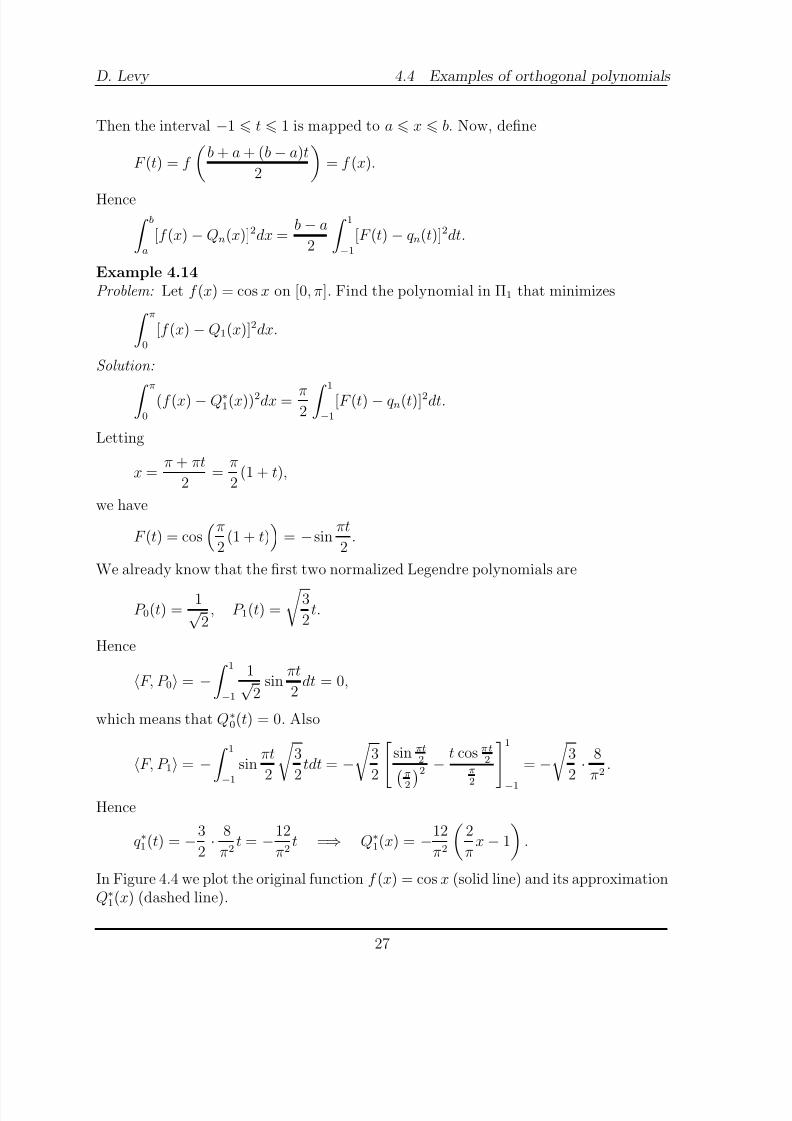
Example 4.13Problem: Let f (x) = cos x on [−1, 1]. Find the polynomial in Π2, that minimizes

1

−1

[f (x)

−Q2(x)]2dx.

Solution: The weight w(x) ≡ 1 on [−1, 1] implies that the orthogonal polynomials weneed to use are the Legendre polynomials. We are seeking for polynomials of degree 2 so we write the first three Legendre polynomials

P 0(x) ≡ 1, P 1(x) = x, P 2(x) = 1

2(3x2 − 1).

The normalization factor satisfies, in general,

1

−1

P 2n(x) = 2

2n + 1

.

Hence 1−1

P 20 (x)dx = 2,

1−1

P 1(x)dx = 2

3,

1−1

P 22 (x)dx = 2

5.

We can then replace the Legendre polynomials by their normalized counterparts:

P 0(x) ≡ 1√ 2

, P 1(x) =

3

2x, P 2(x) =

√ 5

2√

2(3x2 − 1).

We now have

f, P 0 =

1−1

cos x 1√

2dx =

1√ 2

sin x

1

−1

=√

2sin1.

Hence

Q∗

0(x) ≡ sin 1.

25




We also have

f, P 1 =

1−1

cos x

3

2xdx = 0.

which means that Q∗

1(x) = Q∗

0(x). Finally,

f, P 2 =

1−1

cos x

5

2

3x2 − 1

2 =

1

2

5

2(12cos1 − 8sin1),

and hence the desired polynomial, Q∗

2(x), is given by

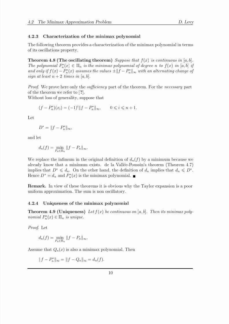
Q∗

2(x) = sin 1 +

15

2 cos1 − 5sin1

(3x2 − 1).

In Figure 4.3 we plot the original function f (x) = cos x (solid line) and its approximation

Q∗2(x) (dashed line). We zoom on the interval x ∈ [0, 1].

0 0.1 0.2 0.3 0.4 0.5 0.6 0.7 0.8 0.9 10.5

0.55

0.6

0.65

0.7

0.75

0.8

0.85

0.9

0.95

1

x

Figure 4.3: A second-order L2-approximation of f (x) = cos x. Solid line: f (x); Dashed

line: its approximation Q∗2(x)

If the weight is w(x) ≡ 1 but the interval is [a, b], we can still use the Legendrepolynomials if we make the following change of variables. Define

x = b + a + (b − a)t

2 .

26




! !"# $ $"# % %"# &

$

!"#

!

!"#

$

x

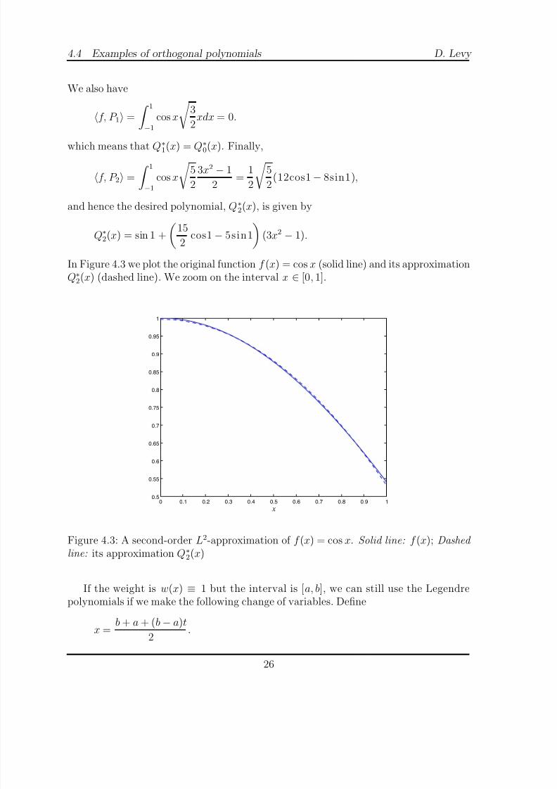
Figure 4.4: A first-order L2-approximation of f (x) = cos x on the interval [0, π]. Solid

line: f (x), Dashed line: its approximation Q∗

1(x)

Example 4.15Problem: Let f (x) = cos x in [0, ∞). Find the polynomial in Π1 that minimizes

∞

0

e−x[f (x) − Q1(x)]2dx.

Solution: The family of orthogonal polynomials that correspond to this weight on[0, ∞) are Laguerre polynomials. Since we are looking for the minimizer of theweighted L2 norm among polynomials of degree 1, we will need to use the first twoLaguerre polynomials:

L0(x) = 1, L1(x) = 1 − x.

We thus have

f, L0w =

∞

0

e−x cos xdx = e−x(− cos x + sin x)

2

∞

0

= 1

2.

Also

f, L1w =

∞

0

e−x cos x(1−x)dx = 1

2−

xe−x(− cos x + sin x)

2 − e−x(−2sin x)

4

∞

0

= 0.

This means that

Q∗

1(x) = f, L0w L0(x) + f, L1w L1(x) = 1

2.

28




4.4.2 Properties of orthogonal polynomials

We start with a theorem that deals with some of the properties of the roots of orthogonalpolynomials. This theorem will become handy when we discuss Gaussian quadratures

in Section ??. We let {P n(x)}n0 be orthogonal polynomials in [a, b] with respect to theweight w(x).

Theorem 4.16 The roots x j, j = 1, . . . , n of P n(x) are all real, simple, and are in

(a, b).

Proof. Let x1, . . . , xr be the roots of P n(x) in (a, b). Let

Qr(x) = (x − x1) · . . . · (x − xr).

Then Qr(x) and P n(x) change their signs together in (a, b). Also

deg(Qr(x)) = r n.

Hence (P nQr)(x) is a polynomial with one sign in (a, b). This implies that

ba

P n(x)Qr(x)w(x)dx = 0,

and hence r = n since P n(x) is orthogonal to polynomials of degree less than n.Without loss of generality we now assume that x1 is a multiple root, i.e.,

P n(x) = (x − x1)2P n−2(x).

Hence

P n(x)P n−2(x) =

P n(x)

x − x1

2

0,

which implies that

b

a

P n(x)P n−2(x)dx > 0.

This is not possible since P n is orthogonal to P n−2. Hence roots can not repeat.

Another important property of orthogonal polynomials is that they can all be writtenin terms of recursion relations. We have already seen specific examples of such relationsfor the Legendre, Chebyshev, and Hermite polynomials (see (4.32), (4.35), and (4.42)).The following theorem states such relations always hold.

29




Theorem 4.17 (Triple Recursion Relation) Any three consecutive orthonormal poly-

nomials are related by a recursion formula of the form

P n+1(x) = (Anx + Bn)P n(x)

−C nP n−1(x).

If ak and bk are the coefficients of the terms of degree k and degree k − 1 in P k(x), then

An = an+1

an, Bn =

an+1

an

bn+1

an+1− bn

an

, C n =

an+1an−1

a2n

.

Proof. For

An = an+1

an,

let

Qn(x) = P n+1(x) − AnxP n(x)

= (an+1xn+1 + bn+1xn + . . .) − an+1

anx(anxn + bnxn−1 + . . .)

=

bn+1 − an+1bn

an

xn + . . .

Hence deg(Q(x)) n, which means that there exists α0, . . . , αn such that

Q(x) =n

i=0

αiP i(x).

For 0 i n − 2,

αi = Q, P iP i, P i = Q, P i = P n+1 − AnxP n, P i = −An xP n, P i = 0.

Hence

Qn(x) = αnP n(x) + αn−1P n−1(x).

Set αn = Bn and αn−1 =

−C n. Then, since

xP n−1 = an−1

anP n + q n−1,

we have

C n = An xP n, P n−1 = An P n, xP n−1 = An

P n,

an−1

anP n + q n−1

= An

an−1

an.

30




Finally

P n+1 = (Anx + Bn)P n − C nP n−1,

can be explicitly written as

an+1xn+1+bn+1xn+. . . = (Anx+Bn)(anxn+bnxn−1+. . .)−C n(an−1xn−1+bn−1xn−2+. . .).

The coefficient of xn is

bn+1 = Anbn + Bnan,

which means that

Bn = (bn+1 − Anbn) 1

an.

approximation chap

Documents