Physics Informed Neural Networks for

Simulating Radiative Transfer

Siddhartha Mishra, Roberto Molinaro ∗

April 6, 2021

Abstract

We propose a novel machine learning algorithm for simulating radiative transfer. Our algorithm isbased on physics informed neural networks (PINNs), which are trained by minimizing the residual ofthe underlying radiative transfer equations. We present extensive experiments and theoretical errorestimates to demonstrate that PINNs provide a very easy to implement, fast, robust and accuratemethod for simulating radiative transfer. We also present a PINN based algorithm for simulatinginverse problems for radiative transfer efficiently.

1 Introduction

The study of radiative transfer is of vital importance in many fields of science and engineering includingastrophysics, climate dynamics, meteorology, nuclear engineering and medical imaging [33]. The funda-mental equation describing radiative transfer is a linear partial integro-differential equation, termed asthe radiative transfer equation. Under the assumption of a static underlying medium, it has the followingform [33],

1

cut + ω · ∇xu+ ku+ σ

(u− 1

sd

∫Λ

∫S

Φ(ω, ω′, ν, ν′)u(t, x, ω′, ν′)dω′dν′

)=f, (1.1)

with time variable t ∈ [0, T ], space variable x ∈ D ⊂ Rd (and DT = [0, T ] × D), angle ω ∈ S = Sd−1

i.e. the d-dimensional sphere and frequency (or group energy) ν ∈ Λ ⊂ R. The constants in (1.1) arethe speed of light c and the surface area sd of the d-dimensional unit sphere. The unknown of interestin (1.1) is the so-called radiative intensity u : DT × S × Λ 7→ R, while k = k(x, ν) : D × Λ 7→ R+

is the absorption coefficient and σ = σ(x, ν) : D × Λ 7→ R+ is the scattering coefficient. The integralterm in (1.1) involves the so-called scattering kernel Φ : S × S × Λ × Λ 7→ R, which is normalized as∫S×Λ

Φ(·, ω′, ·, ν′)dω′dν′ = 1, in order to account for the conservation of photons during scattering.The dynamics of radiative transfer are driven by a source (emission) term f = f(x, ν) : D × Λ 7→ R.

Although the radiative transfer equation (1.1) is linear, explicit solution formulas are only availablein very special cases [33]. Hence, numerical methods are essential for the simulation of the radiativeintensity in (1.1). However, the design of efficient numerical methods is considered to be very challenging[18, 19, 33]. This is on account of the high-dimensionality of the radiative transfer equation (1.1), wherein the most general case of three space dimensions, the radiative intensity is a function of 7 variables(4 for space-time, 2 for angle and 1 for frequency). Traditional grid-based numerical methods such asfinite elements or finite differences, which involve N ` degrees of freedom (for ` dimensions, with N beingthe number of points in each dimension), require massive computational resources to be able to simulateradiative transfer accurately [18, 19]. Moreover in practice, one has to encounter media with very differentoptical properties characterized by different scales in the absorption and scattering coefficients and in theemission term in (1.1), which further complicates the design of robust and efficient numerical methods.

∗Seminar for Applied Mathematics (SAM), D-MathETH Zurich, Ramistrasse 101.

1

arX

iv:2

009.

1329

1v2

[cs

.LG

] 5

Apr

202

1

In spite of the aforementioned challenges, several types of numerical methods have been proposed inthe literature for simulating radiative transfer, see [9, 12, 18, 33] and references therein for a detailedoverview. These include Monte Carlo ray-tracing type particle methods [45], which do not suffer fromthe curse of dimensionality and are easy to parallelize but are characterized by slow convergence (withrespect to number of particles) and are mostly limited to media with fairly uniform optical properties.Discrete Ordinate Methods (DOM), are based on the discretization of the angular domain S with anumber of fixed directions and the resulting systems of spatio-temporal PDEs is solved by finite elementor finite difference methods. Although easy to implement, these methods can be very expensive andalso suffer from the so-called ray effects in optically thin media [23]. Spherical harmonics, based on aseries expansion in the angle, have been widely used in radiative transfer [33]. Although shown to exhibitspectral convergence for smooth solutions [13], these methods are well-known to still suffer from the curseof dimensionality, see [12, 34]. A particular variant of the spherical harmonics, the so-called P1 method,is an example of a class of flux limited diffusion methods [9], which are widely used for optically thickmedia.

Moment based methods lead to another class of numerical methods for simulating radiative transfer,see [9] and references therein. For these methods, one derives a PDE for the so-called incident radiationby integrating (1.1) over the angular domain S. The evolution of the incident radiation is determinedby the heat (radiation) flux, which is also the first angular moment. The evolution of the heat flux hasto be determined from the second angular moment of u, which is termed as the pressure tensor. Thesehierarchy of moments have to be closed by suitable closure relations (see [9] and references therein) andthe resulting PDEs are discretized by finite elements or finite differences. These moment based methodscan lead to inaccurate approximation of the incident radiation, particularly when suitable closures arenot available. Finally in recent years, several attempts have been made to design efficient finite elementmethods for the radiative transfer equation, such as those based on sparse grids [47] or sparse tensorproduct finite element spaces [18, 47]. Although these methods can alleviate the curse of dimensionalityin certain cases, they are rather complicated to implement and can still be computationally expensive,particularly when higher-order elements are used [12].

Summarizing the above discussion, it is fair to conclude that all the proposed methods have somedeficiencies, in particular in their computational cost for simulating realistic problems. Thus, there is apressing need to design a numerical method that is accurate, fast (in terms of computational time), easyto use and able to deal with the high dimensions and optical heterogeneity of the underlying radiativetransfer equation (1.1). We aim to propose such a numerical method in this article.

Our proposed numerical method is based on deep neural networks [10], i.e. functions formed byconcatenated compositions of affine transformations and scalar non-linear activation functions. Deepneural networks have been extremely successful at diverse tasks in science and engineering [24] such asat image and text classification, computer vision, text and speech recognition, autonomous systems androbotics, game intelligence and even protein folding [7]. They are being increasingly used in the contextof scientific computing, particularly for different aspects of numerical solutions of PDEs [6, 14, 27, 28]and references therein.

As deep neural networks possess the so-called universal approximation property or ability to accuratelyapproximate any continuous (even measurable) function [1], they can be used as ansatz (search) spaces forsolutions of PDEs. This property lays the foundation for the so-called Physics informed neural networks(PINNs) which collocate the PDE residual on training points of the approximating deep neural network.First proposed in [21, 22], PINNs been revived and developed in significantly greater detail recently inthe pioneering contributions of Karniadakis and collaborators. PINNs have been successfully applied tosimulate a variety of forward and inverse problems for PDEs, see [5, 15, 17, 25, 26, 29, 36, 39, 40, 41, 43]and references therein.

In recent papers [30] (for the forward problem) and [31] (for the inverse problem), the authors an-alyzed PINNs and provide a rigorous explanation for the efficiency of PINNs, based on stability of theunderlying PDEs. A surprising observation in [30, 31] was the ability of PINNs to overcome the curseof dimensionality, at least for some PDEs. This observation, together with the well-documented abilityof PINNs to approximate PDEs is a starting point of this paper where we adapt PINNs to solve theradiative transfer equation (1.1). The main contributions of the current paper are as follows,

• We present a novel algorithm for approximating the radiative transfer equation (1.1) in a very

2

general setting. Our algorithm is based on suitable physics informed neural networks (PINNs).

• We analyze the proposed algorithm by rigorously proving an estimate on the so-called generalizationerror of the PINN. This estimate shows that as long as the PINN is trained well, it approximatesthe solution of (1.1) to high accuracy.

• We present a suite of numerical experiments to illustrate the accuracy and efficiency of the proposedalgorithm.

• A major advantage of PINNs is their ability to approximate inverse problems (with the same levelof complexity as the forward problem). Hence, we will also modify PINNs to approximate aninverse problem for radiative transfer, namely determining the unknown absorption or scatteringcoefficients in (1.1) from measurements of moments of the radiative intensity.

Thus, we present a novel, fast, robust, accurate and easy to code and implement algorithm for simulatingthe general form of the radiative transfer equations (1.1) and provide analysis and numerical experimentsto demonstrate that this algorithm efficiently approximates both forward and inverse problems for radia-tive transfer. The rest of the paper is organized as follows, in section 2, we describe the PINNs algorithmand provide an estimate on the underlying generalization error. Numerical experiments are presented insection 3, PINNs for inverse problems are described in section 4 and the proposed method and resultsare discussed in section 5.

2 Physics informed neural networks for approximating (1.1)

In this section, we describe the PINNs algorithm for simulating radiative transfer. We start by elaboratingon the underlying PDE (1.1).

2.1 The model.

We model radiative transfer in a static medium by the evolution equation (1.1) for the radiative intensityu. This partial integro-differential equation is supplemented with the initial condition,

u(0, x, ω, ν) = u0(x, ω, ν), (x, ω, ν) ∈ D × S × Λ, (2.1)

for some initial datum u0 : D × S × Λ 7→ R.Given that the radiative transfer equation (1.1) is a transport equation, the boundary conditions are

imposed on the so-called inflow boundary given by,

Γ− = {(t, x, ω, ν) ∈ [0, T ]× ∂D × S × Λ : ω · n(x) < 0} (2.2)

with n(x) denoting the unit outward normal at any point x ∈ ∂D (the boundary of the spatial domainD). We specific the following boundary condition,

u(t, x, ω, ν) = ub(t, x, ω, ν), (t, x, ω, ν) ∈ Γ−, (2.3)

for some boundary datum ub : Γ− 7→ R.Given that the radiative intensity is a function of 2d + 1-variables, it is essential to find suitable

low-dimensional functionals (observables) to visualize and interpret it. To this end, one often considersphysically interesting angular-moments such as the incident radiation (zeroth angular moment) and heatflux (first angular moment) given by,

G(t, x, ν) =

∫S

u(t, x, ω, ν)dω (2.4)

F (t, x, ν) =

∫S

u(t, x, ω, ν)ωdω (2.5)

We note that for many applications of radiative transfer, it is common to consider the steady (time-independent) version of the radiative transfer equation (1.1), which formally results from setting c→∞and dropping the time-derivative term in the left hand side of (1.1).

3

2.2 Quadrature rules and Training points

Quadrature i.e numerical approximation of integrals, is essential for simulating the radiative transferequation (1.1) with PINNs. It is needed for approximating the integral with the scattering kernel in(1.1). Moreover, we follow [30], where quadrature points were used as training points for PINNs.

Given any domain D and an integrable function g : D 7→ R, we need to specify quadrature pointszi ∈ D for 1 6 i 6 N , and quadrature weights wi in order to perform the following approximation,∫

D

g(z)dz ≈N∑i=1

wig(zi). (2.6)

For our specific integrals, we consider Gauss-Legendre quadrature rules [46] for approximating thescattering kernel integral in (1.1). To this end, we choose points zSi = (ωSi , ν

Si ), for 1 6 i 6 NS , with

ωSi ∈ S and νSi ∈ Λ as the Gauss-Legendre quadrature points and the weights wSi are the correspondingquadrature weights for a Gauss-Legendre quadrature rule of order s > 1.

We also need the following training points for the PINNs algorithm,

2.2.1 Interior training points.

We set Sint = {zintj }, for 1 6 j 6 Nint, and zintj = (tintj , xintj , ωintj , νintj ) with tintj ∈ [0, T ], xintj ∈ D,ωintj ∈S, νintj ∈ Λ, for all j. These points are the quadrature points of a suitable quadrature rule with weights

wintj .

If the underlying spatial domain D ⊂ Rd can be mapped to a d-dimensional rectangle, either entirelyor in patches, then we can set the training points zintj as a low-discrepancy Sobol sequence [44] in [0, 1]2d+1,by rescaling the relevant domains. Sobol sequences arise in the context of Quasi-Monte Carlo integration[2] and the corresponding quadrature weights are wintj ≡ 1

Nint, for all j. Note that the QMC quadrature

rule does not suffer from the curse of dimensionality (see section 2.5 for details). In case the geometryof the domain is very complicated, one has simply choose random points, independent and identicallydistributed with the underlying uniform distribution, as training points.

2.2.2 Temporal boundary training points.

We denote Stb = {ztbj }, for 1 6 j 6 Ntb, and ztbj = (xtbj , ωtbj , ν

tbj ) with xtbj ∈ D,ωtbj ∈ S, νtbj ∈ Λ, for all

j. These points are the quadrature points of a suitable quadrature rule with weights wtbj . We can chooseSobol points for logically rectangular domains D or random points to constitute this training set.

2.2.3 Spatial boundary training points.

We denote Ssb = {zsbj }, for 1 6 j 6 Nsb, and zsbj = (ttbj , xtbj , ω

tbj , ν

tbj ) with ttbj ∈ [0, T ], xtbj ∈ ∂D, ωtbj ∈

S, νtbj ∈ Λ, for all j. These points are the quadrature points of a suitable quadrature rule with weights

wsbj . As before, we can choose Sobol points for logically rectangular domains D or random points toconstitute this training set.

2.3 Neural Networks

PINNs are neural networks i.e. given an input y = (t, x, ω, ν) ∈ D = DT × S × Λ, a feedforward neuralnetwork (also termed as a multi-layer perceptron), shown in figure 1, transforms it to an output, througha layers of units (neurons) which compose of either affine-linear maps between units (in successive layers)or scalar non-linear activation functions within layers [10], resulting in the representation,

uθ(y) = CK ◦A ◦ CK−1 . . . . . . . . . ◦A ◦ C2 ◦A ◦ C1(y). (2.7)

Here, ◦ refers to the composition of functions and A is a scalar (non-linear) activation function (appliedto vectors componentwise). A large variety of activation functions have been considered in the machinelearning literature [10]. Popular choices for the activation function A in (2.7) include the sigmoid function,the hyperbolic tangent function and the ReLU function.

4

The affine map in the k-layer is given by,

Ckzk = Wkzk + bk, for Wk ∈ Rdk+1×dk , zk ∈ Rdk , bk ∈ Rdk+1 . (2.8)

For consistency of notation, we set d1 = d = 2d+ 1, for d-space dimensions and dK = 1.Thus in the terminology of machine learning (see also figure 1), our neural network (2.7) consists of

an input layer, an output layer and (K − 1) hidden layers for some 1 < K ∈ N. The k-th hidden layer(with dk neurons) is given an input vector zk ∈ Rdk and transforms it first by an affine linear map Ck(2.8) and then by a nonlinear (component wise) activation σ. A straightforward addition shows that our

network contains

(2d+ 2 +

K−1∑k=2

dk

)neurons. We also denote,

θ = {Wk, bk}, θW = {Wk} ∀ 1 6 k 6 K, (2.9)

to be the concatenated set of (tunable) weights for our network. It is straightforward to check thatθ ∈ Θ ⊂ RM with

M =

K−1∑k=1

(dk + 1)dk+1. (2.10)

Figure 1: An illustration of a (fully connected) deep neural network. The red neurons represent the inputs to the networkand the blue neurons denote the output layer. They are connected by hidden layers with yellow neurons. Each hidden unit(neuron) is connected by affine linear maps between units in different layers and then with nonlinear (scalar) activationfunctions within units.

2.4 Training PINNs: Loss functions and optimization

The neural network uθ (2.7) depends on the tuning parameter θ ∈ Θ of weights and biases. Within thestandard paradigm of deep learning [10], one trains the network by finding tuning parameters θ such thatthe loss (error, mismatch, regret) between the neural network and the underlying target is minimized.Our target is the solution u of the radiative transfer equation (1.1) and we wish to find the tuningparameters θ such that the resulting neural network uθ approximates u.

To do so, we follow [22, 39, 30] and define the following PDE residual Rint,θ = Rint,θ(t, x, ω, ν), forall (t, x, ω, ν) ∈ DT × S × Λ,

Rint,θ :=1

c∂tuθ + ω · ∇xuθ + kuθ + σ

(uθ −

1

sd

NS∑i=1

wSi Φ(ω, ωSi , ν, νSi )uθ(t, x, ω

Si , ν

Si )

)− f. (2.11)

Here, k, σ, f are defined from (1.1) and (ωSi , νSi ) are the Gauss-Legendre quadrature points, with quadra-

ture weights wi of order S.We also need the following residuals for the initial and boundary conditions,

Rtb = Rtb,θ := uθ − u0, ∀(x, ω, ν) ∈ D × S × Λ,

Rsb = Rsb,θ := uθ − ub, ∀(t, x, ω, ν) ∈ Γ−.(2.12)

5

The strategy of PINNs, following [39, 30], is to minimize the residuals (2.11) (2.12), simultaneouslyover the admissible set of tuning parameters θ ∈ Θ i.e

Find θ∗ ∈ Θ : θ∗ = arg minθ∈Θ

(‖Rint,θ‖2L2(DT×S×Λ) + ‖Rsb,θ‖2L2(Γ−) + ‖Rtb,θ‖2L2(D×S×Λ)

). (2.13)

However, the L2 norms in (2.13) involve integrals that cannot be computed exactly and need tobe approximated by suitable quadrature rules. It is exactly the place to recall the different trainingsets, introduced in section 2.2. As these precisely correspond to the quadrature points of an underlyingquadrature rule, we approximate the integrals in (2.13) with the corresponding quadrature rule to definethe following loss function,

J(θ) :=

Nsb∑j=1

wsbj |Rsb,θ(zsbj )|2 +

Ntb∑j=1

wtbj |Rtb,θ(ztbj )|2 + λ

Nint∑j=1

wintj |Rint,θ(zintj )|2 (2.14)

with the residuals Rsb,Rtb and Rint defined in (2.12), (2.11), and wsb, zsb, wsb, zsb, wint, zint being thequadrature weights and training points, defined in section 2.2. Furthermore, λ is a hyperparameter forbalancing the residuals, on account of the PDE and the initial and boundary data, respectively.

It is common in machine learning [10] to regularize the minimization problem for the loss function i.ewe seek to find,

θ∗ = arg minθ∈Θ

(J(θ) + λregJreg(θ)) . (2.15)

Here, Jreg : Θ → R is a weight regularization (penalization) term. A popular choice is to set Jreg(θ) =‖θW ‖qq for either q = 1 (to induce sparsity) or q = 2. The parameter 0 6 λreg � 1 balances theregularization term with the actual loss J (2.14).

The above minimization problem amounts to finding a minimum of a possibly non-convex functionover a subset of RM for possibly very large M . We will follow standard practice in machine learningand solving this minimization problem approximately by either (first-order) stochastic gradient descentmethods such as ADAM [20] or even higher-order optimization methods such as different variants of theLBFGS algorithm [8].

For notational simplicity, we denote the (approximate, local) minimum in (2.15) as θ∗ and the under-lying deep neural network u∗ = uθ∗ will be our physics-informed neural network (PINN) approximationfor the solution u of the PDE (1.1). We summarize the PINN algorithm for approximating radiativetransfer below,

Algorithm 2.1. Finding a physics informed neural network (PINN) to approximate the radiative inten-sity u solving (1.1).

Inputs: Underlying domain DT × S × Λ, coefficients and data for the radiative transfer equation (1.1),quadrature points and weights for underlying quadrature rules, non-convex gradient based optimiza-tion algorithms.

Goal: Find PINN u∗ = uθ∗ for approximating the solution u of (1.1) .

Step 1: Choose the training sets as described in section 2.2.

Step 2: For an initial value of the weight vector θ ∈ Θ, evaluate the neural network uθ (2.7), the PDEresidual (2.11), the boundary residuals (2.12), the loss function (2.15) and its gradients to initializethe underlying optimization algorithm.

Step 3: Run the optimization algorithm till an approximate local minimum θ∗ of (2.15) is reached. The mapu∗ = uθ∗ is the desired PINN for approximating the solution u of the radiative transfer equation.

2.5 Estimates on the generalization error

For the sake of definiteness and simplicity, we consider the spatial domain as D = [0, 1]d, with d being

the spatial dimension. Any rectangular domaind∏i=1

[ai, bi], with ai < bi, for any ai, bi ∈ R can be mapped

6

to [0, 1]d by rescaling. Similarly, logically (patch or block) cartesian domains can be transformed to(0, 1)d by combinations of coordinate transforms. We also rescale time and frequency to set T = 1 andΛ = [0, 1]. Finally, the angular domains can be mapped onto to [0, 1]d−1 by rescaling the underlyingpolar coordinates. Hence, the underlying domain is D = DT × S × Λ = [0, 1]2d+1. Thus, we can chooseour interior training points Sint, temporal boundary training points Stb and spatial boundary trainingpoints Ssb as low-discrepancy Sobol points [2].

Our aim in this section is to derive a rigorous estimate on the so-called generalization error (orapproximation error) for the trained neural network u∗ = uθ∗ , which is the output of the PINNs algorithm2.1. This error is of the form,

EG = EG(θ∗) :=

∫D

|u(t, x, ω, ν)− u∗(t, x, ω, ν)|2dz

12

, (2.16)

with dz = dxdtdωdν denoting the volume measure on D.We follow the recent paper [30] and estimate the generalization error (2.16), in terms of training

errors,

EsbT :=

Nsb∑j=1

wsbj |Rsb,θ∗(zsbj )|2 1

2

, EtbT :=

Ntb∑j=1

wtbj |Rtb,θ∗(ztbj )|2 1

2

, EintT :=

Nint∑j=1

wintj |Rint,θ∗(zintj )|2 1

2

(2.17)Note that the training errors, defined above, correspond to a local minimizer θ∗ of (2.15) and are readilycomputable from the loss function (2.15), during and at the end of the training process.

The detailed estimate on the generalization error in Lemma A.1, together with the assumptions onthe underlying coefficients, functions and neural network, is presented and proved in Appendix A. Wedirect the interested reader to the appendix and focus on the following form of the error estimate (A.3),

(EG)2 6 C1

((EtbT )2 + c(EsbT )2 + c(EintT )2

)+ C2

((log(Ntb))

2d

Ntb+ c

(log(Nsb))2d

Nsb+ c

(log(Nint))2d+1

Nint+ cN−2s

S

),

(2.18)

with finite constants C1 = C, C2 = CC∗ defined in (A.4). The following remarks about the bound (2.18)are in order,

Remark 2.2. The estimate (2.18) bounds the generalization error in terms of the training errors definedin (2.17) and the number of training points Nint,sb,tb as well as quadrature points NS for approximatingthe scattering integral in (1.1). Although we have no apriori estimate on the training errors, as arguedin [30], these errors can readily calculated after the training process has completed. Thus, the estimate(2.18) tells us that under the assumptions that the constants appearing in (2.18) are finite, as long asthe PINN is trained well, it generalizes well. This is exactly in the spirit of generalization results intheoretical machine learning [35]. �

Remark 2.3. We see from the right hand side of the bound (2.18) that the dimensional dependence ofthe upper bound is only a logarithmic factor. This is not a severe restriction in this case, as the spatialdimension d is atmost 3. It is well known [2] that the logarithmic factor in the rhs of (2.18) starts affectingthe rate of decay only when Nint < 22d+1. Thus as long as Nint > 128 and Ntb, Ntb > 64, we should see alinear decay in the error contributions of the Sobol points in (2.18). Hence, we claim that as long as thetraining errors do not depend on the underlying dimension, the estimate (2.18) suggests that the PINNsalgorithm 2.1 will not suffer from a curse of dimensionality. �

Remark 2.4. The estimate (2.18) brings out the role of the speed of light c very clearly. As long as c isfinite, we can rescale time to set c = 1. Nevertheless, the constant C in (2.18) grows exponentially withthe rescaled time, deteriorating the control on the error provided by the bound (2.18). Thus, this boundis not suitable for steady-state problems (formally) obtained by letting c→∞. Nevertheless, a modifiederror estimate can be derived for the steady state case and we present it in the appendix B. �

7

3 Numerical Experiments

3.1 Implementation

The PINNs algorithm 2.1 has been implemented within the PyTorch framework [37] and the code canbe downloaded from https://github.com/mroberto166/RadiativeTransportPinns. As is well doc-umented [39, 40, 30], the coding and implementation of PINNs is extremely simple, particularly whencompared to standard methods such as finite elements. Only a few lines of Python code suffice for thispurpose. All the numerical experiments were performed on a single GeForce GTX1080 GPU.

The PINNs algorithm has the following hyperparameters, the number of hidden layers K − 1, thewidth of each hidden layer dk ≡ d in (2.7), the specific activation function A, the parameter λ in the lossfunction (2.14), the regularization parameter λreg in the cumulative loss function (2.15) and the specificgradient descent algorithm for approximating the optimization problem (2.15). We use the hyperbolictangent tanh activation function, thus ensuring that all the smoothness hypothesis on the resulting neuralnetworks, as required in lemmas A.1 and B.1 are satisfied. Moreover, we use the second-order LBFGSmethod [8] as the optimizer. We follow the ensemble training procedure of [28] in order to choose theremaining hyperparameters. To this end, we consider a range of values, shown in Table 1, for the numberof hidden layers, the depth of each hidden layer, the parameter λ and the regularization parameter λreg.For each configuration in the ensemble, the resulting model is retrained (in parallel) nθ times with differentrandom starting values of the trainable weights in the optimization algorithm and the one yielding thesmallest value of the training loss is selected.

K − 1 d λ λreg nθ

Example 3.2, 3.3 4, 8 16, 20, 24 0.1, 1, 10 0 5

Example 3.4 4, 8 16, 20 0.1, 1 0, 10−6, 10−5 10

Example 3.5 4, 8, 12, 16, 20 16, 20, 24, 28, 32, 36, 40 0.1, 1 0 20

Example 4.2 4, 8 16, 20, 24 1, 10 0 5

Table 1: Hyperparameter configurations and number of retrainings employed in the ensemble training of PINNs for theradiative transfer equation (1.1)

3.2 Monochromatic stationary radiative transfer in one space dimension

We begin with the much simpler case of steady state radiative transfer in the one space dimension, alsoreferred to as slab geometry [9]. In this case, the radiative transfer equations (1.1) simplify to,

µ∂

∂xu(x, µ) +

(σ(x) + k(x)

)u(x, µ) =

σ(x)

2

∫ 1

−1

Φ(µ, µ′)u(z, µ)dµ′, µ = cos(θ), (x, µ) ∈ [0, 1]× [−1, 1].

(3.1)We follow the setup of [38] where the authors benchmarked least squares finite element methods forone-dimensional radiative transfer on this problem. As in [38], the following inflow boundary conditionsare imposed:

u(0, µ) = 1, µ ∈ (0, 1],

u(1, µ) = 0, µ ∈ [−1, 0).(3.2)

Note that the boundary conditions allow for possible discontinuities at µ = 0. The coefficients andscattering kernel are,

σ(x) = x, k(x) = 0, Φ(µ′, µ) =

L∑`=0

d`P`(µ)P`(µ′), d0 = 1, (3.3)

with P`(µ) denoting the Legendre polynomial of order `. We employ the sequence of coefficients d` ={1.0, 1.98398, 1.50823, 0.70075, 0.23489, 0.05133, 0.00760, 0.00048}, proposed in [38]. Although only in 2

8

Nint Nsb K − 1 d λ ET ||u− − u∗−||L2 ||u+ − u∗+||L2 Training Time

8192 2048 8 24 0.1 0.00016 0.07 % 0.29 % 57 min

Table 2: Results for monochromatic stationary radiative transfer in one space dimension.

dimensions, this problem is nevertheless considered rather challenging on account of the possible presenceof discontinuities.

We use the PINNs algorithm 2.1 to approximate (3.1), with Sobol points for the interior trainingset Sint and spatial boundary training set Ssb. Similarly, a Gauss-Legendre quadrature rule of order20 is used for approximating the integral with the scattering kernel. We set Nint = 8192, Nsb = 2048and NS = 10, for this experiment. The hyperparameters that resulted from the ensemble training arepresented in Table 2. As seen from the table, a very low training error is obtained in this case. A contourplot of the resulting radiative intensity in (x, µ)-plane is presented in figure 2. The results are very similarto those obtained with a least squares finite element method in [38] (compare figure 2 with figure 3 of[38]). It is interesting to note that this very good qualitative match with the least-squares finite elementmethod is obtained with a training time of slightly less than 1 hour.

Figure 2: Contour plot of the radiative intensity u(x, µ) for the 1D monochromatic experiment

Another attractive feature of this simplified problem lies in the fact that the authors in [4] obtainedan exact analytical solution for it. Although it is very complicated to evaluate this solution for thewhole (x, µ)-plane, its values on the boundaries can be readily evaluated i.e. we can readily computeu−(µ) = u(0, µ) and u+(µ) = u(1, µ). We do so and compare the exact solution with the trained PINN,denoted by u∗±. These results are plotted in figure 3. We see from this figure that the PINN is able to veryaccurately approximate the discontinuous exact solution at the boundary. A quantitative comparison inperformed by computed the errors u± − u∗± in L2-norm. These errors, presented in table 2, are verysmall for both boundaries and further demonstrate that the PINN is able to approximate the underlyingdiscontinuous solution to high-accuracy, at very low computational cost. One can possibly further reducethe error by using adaptive activation functions as suggested in [16]. However, we did not observe anyfurther reduction in the already low training error by using adaptive activation functions.

9

Figure 3: Comparison of the analytical and PINNN radiative intensity at the physical domain boundaries for the stationarymonochromatic radiative transfer in one-space dimension.

3.3 Monochromatic stationary radiative transfer in three space dimensions

Next, we consider a monochromatic and stationary version of the general radiative transfer equations(1.1), but in three space dimensions. Already, this problem is in 5 dimensions and is challenging on accountof possibly high computational cost. We use the same setup as in [12] (section 8.2, experiment 3) andconsider the problem in the unit cube D = [0, 1]3 where a source, located at the center c = (0.5, 0.5, 0.5),radiates into the surrounding medium. We consider no further radiation entering the domain (zeroDirichlet boundary conditions). The source term f is given by

f(x) = k(x)Ib(x), Ib(x) =

{0.5− r, r 6 0.50, otherwise

(3.4)

with r = |x − c|. The absorption coefficient is k(x) = Ib(x) and isotropic scattering Φ = 1, with unitscattering coefficient σ(x) = 1 is considered.

As before, we use Sobol points for the interior training set Sint and boundary training set Ssb. Quadra-ture points, corresponding to a Gauss quadrature rule of order 20 are also used. We set Nint = 16384,Nsb = 12288 and NS = 100. The hyperparameters, corresponding to the best performing networks, thatresult from ensemble training are presented in Table 3. We see from this table that this hyperparameterconfiguration resulted in a very low (total) training error of 4.4 × 10−4, which is comparable to thoseobtained in the one-space dimension case (see table 2).

Nint Nsb K − 1 d λ ET Training Time

16384 12288 8 24 0.1 0.00044 1 hr 9 min

Table 3: Results of the ensemble training for the stationary monochromatic radiative transfer in three space dimensions.

As there is no analytical solution available for the radiative intensity in this case, we cannot computegeneralization errors. However, based on the theory (see estimate (A.3)) and on the comparison withthe one-dimensional case, we expect very low generalization errors when the training errors are this low.Moreover, we can perform qualitative comparisons with the results obtained in [12] with an efficientdiscrete ordinate method. To this end, we plot three-dimensional volume plot for the incident radiationG(x) (see the first equation in (2.4) for definition) in figure 4. We see from this figure that the results withPINN are very similar to the results with the discrete ordinate method, shown in [12] (figure 8.12, page126). Thus, we are able to approximate the incident radiation to the same accuracy as a discrete ordinatemethod. The main differences lies in the simplicity of implementation and very low computational cost.We observe from table 3 that the PINN was trained in approximately 70 minutes on a single GPU.This should be contrasted with the very intricate parallel algorithm of [12], which required considerably

10

more computational time as the method resulted in very number of degrees of freedom ranging from200000− 600000.

Figure 4: Contour plot of the incident radiation G(x) for the 3D monochromatic experiment

3.4 Polychromatic stationary radiative transfer in three space dimensions

Next, we consider the most general case of the steady state radiative transfer equation (B.1) by followingthe setup of [42] and references therein, where (B.1) is considered in the unit cube D = [0, 1]3 and in thefrequency domain Λ = [−6, 6], with normalization of energy groups. Furthermore, we consider a simplecase of zero absorption, isotropic kernel, zero Dirichlet boundary conditions and spherical symmetry.Under the assumptions, by integrating equation (B.1) over the unit sphere S, we arrive at the followingordinary differential equation for the radial flux i.e the incident heat flux (2.4) along the radius,

∇ · Fr =1

r2

d

drr2Fr = 4πf(r, ν) (3.5)

with r = |x− (0.5, 0.5, 0.5)| (see also [42] and references therein).An exact solution for the above ODE can be easily obtained. In particular, with the source term:

f(x, ν) =

{√πϕ(ν)

(1− 2r

)if r 6 0.5,

0 otherwise,ϕ(ν) =

1√π

exp(− ν2

), (3.6)

the radial flux Fr results in

Fr =

{4√π3ϕ(ν)

(r3 −

r2

2

)if r 6 0.5,

4√π3ϕ(ν) 1

96r2 otherwise.(3.7)

As in the previous numerical experiment, we use Sobol points for the interior and boundary training setsand Gauss quadrature points for integrating the scattering kernel, with Nint = 16384, Nsb = 12288 andNS = 100. The hyperparameters used in the ensemble trainig are reported in table 1 and the resultingbest performing configuration is shown in table 4. We observe from this table that the resulting trainingerror is 1.6 × 10−3, which is about three times higher than the training error with the monochromaticexperiment (see table 3). This is not surprising as the underlying problem is more complicated on accountof introducing frequency as an additional variable and resulting in a 6-dimensional problem.

11

As no analytical solution is available for the radiative intensity, we cannot compute the generalizationerror (B.4). However, we can compute the error between the analytical radial flux (3.7) and the PINNapproximation (computed from the intensity with a Gauss-Legendre quadrature rule). We show theresulting L2-norm of the error in table 4. We see from this table that the error for the flux is quite lowat approximately 2% relative error, even for this rather complicated underlying problem. Moreover, thetraining time is only one hour. Thus, PINNs are able to approximate the underlying solution to highaccuracy at low computational cost for this 6-dimensional problem.

Nint Nsb K − 1 d λ ET ||Fr − F ∗r ||L2 Training Time

16384 12288 8 20 0.1 0.0016 2.1 % 1 hr 6 min

Table 4: Results for steady polychromatic radiative transfer in three space dimensions.

3.5 Polychromatic time-dependent Radiative transfer in three space dimen-sions

For the final numerical experiment, we consider the configuration proposed in [11], which is widely used inbenchmarking the radiative transport modules in production codes for radiation-(magneto)hydrodynamics,in the context of Astrophysics [48]. The setup is as follows; a sphere with radius Ri and fixed temperatureTS is surrounded by a cold static medium at temperature Tm < TS . The experiment might represent, forinstance, the model of a star radiating in the surrounding atmosphere. It is assumed that the sphere, aswell as the surrounding medium, are emitting with a Planckian distribution

B(T, ν) =2hν3

c21

ehνkbT − 1

(3.8)

with h and kb being the Planck and Boltzmann constant, and c the speed of light.To make the problem tractable, the authors of [11] neglect scattering entirely by setting σ ≡ 0.

Moreover, the absorption coefficient is modeled by k(x, ν) = kν , with ν being the frequency. The emissionterm is modeled by f(x, ν) = kνB(Tm, ν), resulting in the following form of the radiative transfer equation(1.1),

1

c

∂u

∂t+ ω · ∇xu = kν(B(Tm, ν)− u), (t, x, n, ν) ∈ DT × S × Λ. (3.9)

In the context of radiation-(magneto)hydrodynamics, one is mostly interested in the angular momentsof the radiative intensity that naturally arise in calculating the contridbution of radiation to the totalenergy of the fluid (plasma). Hence, it is customary to integrate (3.9) over the sphere S to derive thefollowing PDE for incident radiation (2.4):

1

c

∂

∂tG+∇x · F = kν

(b(Tm, ν)−G

), (t, x, ν) ∈ DT × Λ. (3.10)

with b(T, ν) = 4πB(T, ν).However, the PDE (3.10) is not closed and one needs a closure for the flux F in terms of the incident

radiation G. It is common practice in astrophysics to use the so-called diffusion approximation of theflux [3]:

F (t, x, ν) = − 1

3kν∇G(t, x, ν), (3.11)

resulting in the following PDE,

1

c

∂

∂tG− 1

3kν∆G = kν

(b(Tm, ν)−G

), (t, x, ν) ∈ DT × Λ. (3.12)

Defining the Knudsen number K = Lkν (with L being a characteristic length scale), it is well known thatthe diffusion approximation is justified in the limit of K →∞.

12

kν Nint Nsb Ntb K − 1 d λ ET Training Time

1 16384 12288 12288 4 40 0.1 0.0028 3 hr 25 min

10 16384 12288 12288 4 40 0.1 0.012 2 hr 15 min

Table 5: Results for polychromatic time-dependent radiative transfer in three space dimensions.

Although the PDE (3.12) is simpler than the full radiative transfer equation (1.1), efficient numericalapproximation of (3.12) is still quite challenging as the incident radiation is a function of 5 variables. Asit happens, PINNs provide an efficient method for approximating high-dimensional parabolic equationssuch as (3.12), see [30] section 3 for details.

However, by assuming radial symmetry and with the flux approximation given in (3.11), the differentialequation (3.12) admits an analytical solution satisfying the initial and boundary conditions

G(0, r, ν) = b(Tm, ν),

G(t, r →∞, ν) = b(Tm, ν),

G(0, Ri, ν) = b(Ts, ν).

(3.13)

The exact solution for (3.12) then reads [11],

G(t, r, ν) =b(Tm, ν) +Rir

(b(Ts, ν)− b(Tm, ν)

)F (t, r, ν),

F (t, r, ν) =1

2exp (−3kν(r −R))

{Erfc

(√3kν4ct

(r −R)−√kνct

)+ Erfc

(√3kν4ct

(r −R) +√kνct

)}.

(3.14)For this numerical experiment, we will approximate the full time-dependent radiative transfer equa-

tions (3.9) with the PINNs algorithm 2.1. To this end, we consider (3.9) in the spatial domain D enclosedbetween two spheres with radii Ri = 2 and Re = 4. Moreover, we introduce an auxiliary temporal vari-able τ = ct to rescale time to [0, 1], whereas the energy group ranges between 1015 and 1018. We setTs = 150eV and Tm = 120eV .

The PINNs algorithm 2.1 employs Sobol points in the interior, spatial and temporal boundary trainingsets and we set Nint = 16384, Nsb = Ntb = 12228. Moreover, we solve this problem for two differentvalues of the (constant in frequency) absorption coefficient i.e kν = 1 and kν = 10, resulting in twodifferent Knudsen numbers of K = 2 and K = 20, respectively. Given the challenging nature of thisproblem, we choose slightly different ranges of the hyperparameters, presented in tabel 1 for ensembletraining and also use 20 retrainings, corresponding to different random starting values for the weightsand biases in the training procedure. The resulting best performing configurations are reported in table5. We observe from this table that PINNs provide a very low training error of 2.8× 10−3, for the K = 2case. This training error is comparable to the training errors for the previous two examples. The trainingerror increases by a factor of 4 for the K = 20 case, but still remains relatively low.

As we do not have exact analytical formulas for the full radiative intensity, it is not possible to computegeneralization errors. However to ascertain the quality of the solution, we compare with the exact solution(3.14) of the diffusion equation (3.12) for the incident radiation. This comparison is shown as contourplots for the incident radiation in the (r, ν)-plane (with r denoting the radial direction) in figure 5 aswell as one-dimensional cross-sections for different values of the radius r in figure 6. As seen from boththese figures, there is good agreement between the incident radiation, computed by a Gauss quadratureof the PINN approximation to the radiative intensity in (3.9), and the analytical solution of the diffusionapproximation (3.12) for the K = 20 case. This is not unexpected as the diffusion approximation isaccurate for large Knudsen numbers. On the other hand, there is a significant difference between thethe incident radiation, computed by a Gauss quadrature of the PINN approximation to the radiativeintensity in (3.9), and the analytical solution of the diffusion approximation (3.12) for the K = 2 case.This follows from the fact that the diffusion approximation will provide a poor approximation of (3.9)for low Knudsen numbers. On the other hand, given the relatively low training error as well as the errorestimate (A.3), coupled with the results of the previous numerical experiments, we argue that the PINN

13

(a) Exact solution of (3.12) for kν = 1 (b) PINN for kν = 1

(c) Exact solution of (3.12) for kν = 10 (d) PINN at τ = 1 for kν = 10

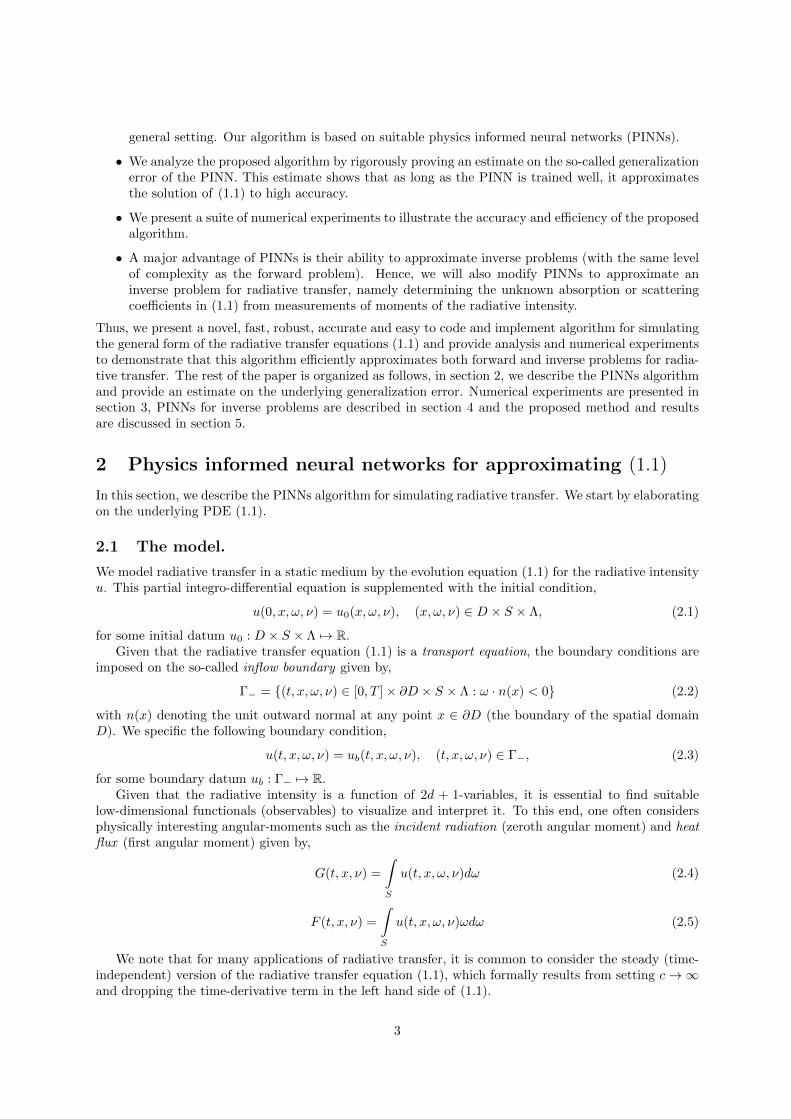
Figure 5: Comparison of incident radiationn with respect to the exact solution of the diffusion approximation (3.12) andPINN approximation of the full radiative transfer equation (3.9) at rescaled time τ = 1 for two different values of theabsorption coefficient kν = 1, 10

provides a much more accurate approximation to the underlying radiative intensity (and its moments)than the diffusion approximation will do, atleast for low to moderate Knudsen numbers. Hence, PINNsprovide a viable and accurate method for competing radiative transfer in media with different opticalproperties. Moreover, the runtime for even this very complicated problem was reasonably small, rangingfrom two to three and half hours on a single GPU.

4 PINNs for the Inverse problem for radiative transfer

One of the most notable features of PINNs is their ability to approximate solutions of inverse problems,with the same accuracy and computational cost as that of forward problems for PDEs. Moreover, thecode for inverse problems ends up being a very minor modification to the code for forward problems,which makes PINNs extremely attractive for various applications [40, 41] and references therein.

Here, we focus on the following inverse problem for radiative transfer. We consider the full time-dependent version on the radiative transfer equation (1.1), with initial and boundary conditions (2.3).The inverse problem is to compute unknown absorption coefficients k, scattering coefficients σ, scatteringkernel Φ or emission term f , given measurements of either the full radiative intensity u or its angularmoments, such as the incident radiation G or heat flux F (2.4). For simplicity of exposition, we choosethe following concrete inverse problem;Given measurements of the incident radiation G(t, x, ν), find the unknown absorption coefficient k =

14

(a) Solution of (3.9) and (3.10) for kν = 1 (b) Solution of (3.9) and (3.10) for kν = 10

Figure 6: Comparison of exact solutions of the diffusion approximation (3.12) with the PINN approximation of the fullradiative transfer equation (3.9) for two different values of the absorption coefficient kν = 1, 10 at different radial locationsand at rescaled time τ = 1

k(x, ν) and the resulting radiative intensity u(t, x, ω, ν) which solves the radiative transfer equation (1.1)with initial and boundary conditions (2.3).

Other combinations of the measured and unknown quantities can be similarly considered. Clearly thisinverse problem is ill-posed as multiple absorption coefficients might lead to the same incident radiation.However, we will aim to obtain one of the possible absorption coefficients, consistent with the measuredincident radiation.

To this end, we slightly modify the PINNs algorithm as described below,

4.1 PINNs for the inverse problem

Following [40, 31], we seek to find the deep neural networks kθk : D×Λ 7→ R+ and uθu : DT ×S×Λ 7→ R,with the concatenated parameter vector θ = {θk, θu} ∈ Θ, approximating the absorption coefficient andradiative intensity, respectively.

In addition to the interior training set Sint, spatial boundary training set Ssb and temporal boundarytraining set Stb, defined in section 2, we also required the so-called data training set Sd = {ydj }, for

1 6 j 6 Nd, and ydj ∈ DT × Λ.The residuals for initial and boundary conditions are given by Rtb,Rsb (2.12). We slightly modify the

PDE residual (2.11) to,

Rint,θ :=1

c∂tuθu + ω · ∇xuθu + kθkuθu + σ

(uθu −

1

sd

NS∑i=1

wSi Φ(ω, ωSi , ν, νSi )uθu(t, x, ωSi , ν

Si )

)− f. (4.1)

We also need the data residual,

Rd,θ := G (uθu)− G(t, x, ν), ∀(t, x, ν) ∈ DT × Λ, (4.2)

with G being the incident radiation calculated from (2.4) with a Gauss quadrature approximation of theangular integral and G being the measured incident radiation.

The resulting loss function is,

J(θ) :=

Nd∑j=1

wdj |Rd,θ(ydj )|2 +

Nsb∑j=1

wsbj |Rsb,θ(zsbj )|2 +

Ntb∑j=1

wtbj |Rtb,θ(ztbj )|2 + λ

Nint∑j=1

wintj |Rint,θ(zintj )|2 (4.3)

with the residuals Rd,Rsb,Rtb and Rint defined in (4.2), (2.12) ,(2.11), and wd, yd, wsb, zsb, wsb, zsb,wint, zint being the quadrature weights and training points, corresponding to the data, boundary andinterior training sets.

15

The PINNs algorithm for the inverse problem is summarized as,

Algorithm 4.1. Finding physics informed neural network (PINNs) to approximate the absorption co-efficient k and radiative intensity u solving the radiative transfer equation (1.1), and consistent withmeasured data G for the incident radiation

Inputs: Underlying domain DT × S × Λ, coefficients and data for the radiative transfer equation (1.1),measured incident radiation G, quadrature points and weights for underlying quadrature rules, non-convex gradient based optimization algorithms.

Goal: Find PINN (k∗, u∗) =(kθ∗k , uθ∗u

)for approximating the inverse problem for radiative transfer

Step 1: Choose the training sets as described in section 2.2 and in this subsection.

Step 2: For an initial value of the weight vector θ ∈ Θ, evaluate the neural networks uθu , kθk (2.7), thePDE residual (4.1), the data residual (4.2), the boundary residuals (2.12), the loss function (4.3)and its gradients to initialize the underlying optimization algorithm.

Step 3: Run the optimization algorithm till an approximate local minimum θ∗ of (4.3) is reached. The mapu∗ = uθ∗u is the desired PINN for approximating the solution u of the radiative transfer equationand the map k∗ = kθ∗k is the corresponding absorption coefficient.

Nint Nsb Nd K − 1 d λ ET ||u− u∗||L2 ||k − k∗||L2 ||G−G∗||L2 Training Time

16384 120 4096 8 20 1.0 0.00094 0.65 % 2.8 % 0.073% 1 hr 44 min

Table 6: Results for the inverse problem for radiative transfer.

4.2 A Numerical Experiment.

The monochromatic stationary version of the radiative transfer equation (1.1) in three space dimensions,is used in this numerical experiment. The spatial domain is the unit cube D = [0, 1]3, with scatteringcoefficient σ = 0.5, scattering kernel Φ ≡ 1. The source term f and boundary term ub are generatedusing the following synthetic absorption coefficient and exact solution,

k(x) =

3∏i=1

x2i , u(x, ω) =

3

16π(1 + (ω · ω′)2)

3∏i=1

xi(xi − 1), n′ =( 1√

3,

1√3,

1√3

)T(4.4)

The measured incident radiation G in (4.2) is calculated from the radiative intensity u above by usingthe formula (2.4).

For this numerical experiment, we also impose boundary conditions on the neural network approx-imating the absorption coefficient kθk to approximately match the values of k, defined in (4.4) on theboundary of D, leading to an additional term in (4.3). Finally, in order to ensure uniqueness of theabsorption coefficient, we include in the loss function, the so-called Tikhonov regularization:

JT (θ) = λk||∇kθ||22, λk = 0.001. (4.5)

We use Sobol points for the interior training points and uniformly distributed random points are usedas data training points, with Nint = 16384, Nd = 4096. The resulting best performing hyperparameterconfiguration after ensemble training is presented in Table 6.

In figure 7 we plot the incident radiation G and the absorption coefficient k, along the diagonalof the unit cube, computed with the PINNs algorithm 4.1. As observed from this figure, the incidentradiation is almost identical to the measured data G. This is further verified from table 6, from whichwe observe a very low L2-error for the incident radiation. On the other hand, the absorption coefficientagrees reasonably well with the ground truth in (4.4), with an error of less than 3%. Also the radiativeintensity is approximated to very high accuracy, with a generalization error below 1%. This is even moreimpressive if one consider that the problem is solved with a computational time of approximately 100minutes.

16

(a) Incident radiation G (b) Absorption Coefficient k

Figure 7: Results for the PINNs algorithm 4.1 for the inverse problem for radiative transfer. The PINNs approximationto the incident radiation and absorption coefficient are plotted along the diagonal of the unit cube and compared with themeasured data G and ground truth absorption coefficient k given by (4.4).

5 Discussion

Accurate numerical approximation of the radiative transfer equations (1.1) is considered very challengingas the underlying problem is high-dimensional, with 7-dimensions in the most general case. Moreover,the presence of different physical effects such as emission, absorption and scattering as well as varyingoptical parameters in the surrounding medium further complicates design of efficient numerical algo-rithms. As discussed in the introduction, existing numerical methods can suffer from the so-called curseof dimensionality and require very large amount of computational resources to achieve desired accuracy.

Hence, there is a need for designing algorithms for simulating radiative transfer, that are easy toimplement and fast (in terms of computational run time) while still being accurate. We proposed suchan algorithm in this article. Our algorithm 2.1 is based on physics informed neural networks (PINNs)i.e. deep neural networks for approximating the radiative intensity in (1.1). The deep neural networkis trained by using a gradient descent method to minimize a loss function (2.15), that consists of thePDE residual, resulting from the neural network being plugged into the radiative transfer equation (1.1).Mismatches with respect to the initial and boundary conditions also contribute to the loss function. Theresiduals are collocated at training points, which correspond to quadrature points with respect to anunderlying quadrature rule. We chose Sobol low-discrepancy sequences as training points in order toalleviate the curse of dimensionality.

The resulting algorithm is extremely simple to code within standard machine learning frameworkssuch as TensorFlow and Pytorch. We presented a suite of numerical experiments ranging from thesimplest monochromatic stationary radiative transfer in one space dimension (3.1) to the most generaltime-dependent polychromatic radiative transfer in three space dimensions. PINNs performed very wellon all the numerical experiments, leading to low errors with small run (training) times. In particular, theresults were qualitatively and quantitatively comparable to published results, but possibly at a fractionof the cost. The experimental results were supplemented with rigorous error estimates that boundedthe generalization error (2.16) in terms of computable training errors (2.17) and number of quadraturepoints, independent of the underlying dimension, see bounds (A.3) for details. The predictions of theerror estimates were validated by the experiments.

Hence, we claim that the PINNs algorithm 2.1 is a general purpose, simple to implement, fast andaccurate simulator for radiative transfer. Moreover, we also presented a (very) slightly modified versionof the PINN algorithm to efficiently simulate a class of inverse problems for radiative transfer. In thisproblem, the objective is to compute the unknown absorption coefficient from measurements of theincident radiation. To this end, we proposed the deep neural network based algorithm 4.1, which addeda data fidelity term (4.2) to the underlying loss function (4.3). This algorithm was also found to be both

17

fast and accurate in numerical experiments. Thus, we provide novel machine learning algorithms whichare fast, easy to implement and accurate for efficiently simulating different aspects of radiative transfer.

This article should be considered as a first step in adapting machine learning algorithms for simulatingradiative transfer. The proposed algorithm lends itself readily to be extended in the following directions,

• The quantities of interest in many applications of radiative transfer, particularly in astrophysics, areangular moments such as the incident radiationG and heat flux F , defined in (2.4) as these quantitiesdefine the contribution of radiation to the total energy. Thus, in radiation hydrodynamics, one oftenresorts to using moment models. However, these moment models require closure relations, whichmight either be expensive to compute and/or inaccurate (see section 3.5 for a simple diffusion basedclosure). Given the computational speed of PINNs, one can readily employ algorithm 2.1 as theradiation module in a hydrodynamics code, with angular moments and the resulting energy beingcomputed from the neural network approximation of the radiative intensity. Another option wouldbe to leverage the ability of PINNs to directly perform hydrodynamic simulations (see [41, 30]) andhave a full PINN simulation of radiation hydrodynamics. Both approaches should be developedand tested.

• We covered the inverse problem for radiative transfer briefly in section 4. Algorithm 4.1 can bereadily extended to many other inverse problems involving radiative transfer, for instance findingemission and scattering coefficients from measurements of incident radiation and heat fluxes at afew points. A careful exposition and analysis of the resulting algorithms and their application inpractical contexts will be the basis of future papers.

Acknowledgements

The research of SM and RM was partially supported by the European Research Council (ERC) underERCCoG 770880 COMANFLO. SM thanks Dr. Roger Kappeli of SAM, ETH Zurich for his inputs onradiation and astrophysics.

A Estimates on the generalization error for the radiative trans-fer equation (1.1)

In order to derive an error estimate for the PINNs algorithm, we need to make some assumptions on thescattering kernel Φ in (1.1). We follow standard practice and assume that it is symmetric Φ(ω, ω′, ν, ν′) =Φ(ω′, ω, ν′, ν). Moreover, the following function,

Ψ(ω, ν) =

∫S×Λ

Φ(ω, ω′, ν, ν′)dω′dν′, (A.1)

is essentially bounded i.e. Ψ ∈ L∞(S × Λ). We have the following estimate on the generalization error(2.16),

Lemma A.1. Let u ∈ L2(D) be the unique weak solution of the radiative transfer equation (1.1), withabsorption coefficient 0 6 k ∈ L∞(D × Λ), scattering coefficient 0 6 σ ∈ L∞(D × Λ) and a symmetricscattering kernel Φ ∈ C`(S × Λ× S × Λ), for some ` > 1, such that the function Ψ (defined in (A.1)) isin L∞(S × Λ). Let u∗ = uθ∗ ∈ C`(D) be the output of the PINNs algorithm 2.1 for approximating theradiative transfer equation (1.1), such that

max{VHK(u∗), VHK (Rint,θ∗)} < +∞, (A.2)

with VHK being the so-called Hardy-Krause variation (see [2, 32] for the precise definition). We alsoassume that the initial data u0 and boundary data ub are of bounded Hardy-Krause variation. Then,under the assumption that Sobol points are used as the training points Sint, Ssb, Stb in algorithm 2.1 and

18

Guass-quadrature rule of order s = s(`) is used in approximating the scattering kernel in the residual(2.11), we have the following estimate on the generalization error,

(EG)2 6 C((EtbT )2 + c(EsbT )2 + c(EintT )2

)+ CC∗

((log(Ntb))

2d

Ntb+ c

(log(Nsb))2d

Nsb+ c

(log(Nint))2d+1

Nint+ cN−2s

S

)(A.3)

with constants defined as,

C = T + cCT 2ecCT , C = 2 +2(‖σ‖L∞ + ‖Ψ‖L∞)

sd

C∗ = max{VHK

((R∗tb)

2), VHK

((R∗sb)

2), VHK

((R∗int)

2), C}

C = C (|D|, ‖Φ‖C` , ‖u∗‖C`)

(A.4)

Proof. We drop the θ∗ dependence in the residuals (2.11), (2.12), for notational convenience and denotethe residuals as R∗int,R

∗sb,R

∗tb. Define,

E(u∗,Φ) :=

NS∑i=1

wSi Φ(ω, ωSi , ν, νSi )u∗(t, x, ωSi , ν

Si )−

∫Λ

∫S

Φ(ω, ω′, ν, ν′)u∗(t, x, ω′, ν′)dω′dν′. (A.5)

It is straightforward to derive from the radiative transfer equation (1.1) and the definition of residuals(2.11), (2.12), that the error u = u∗ − u, satisfies the following integro-differential equation,

1

cut + ω · ∇xu = −(k + σ)u+

σ

sd

∫Λ

∫S

Φ(ω, ω′, ν, ν′)u(t, x, ω′, ν′)dω′dν′

+ R∗int + E(u∗,Φ).

u(0, x, ω, ν) = R∗tb, (x, ω, ν) ∈ D × S × Λ,

u(t, x, ω, ν) = R∗sb, (t, x, ω, ν) ∈ Γ− × Λ.

(A.6)

Multiplying u on both sides of the first equation in (A.6), we obtain,

1

2c

d(u2)

dt+ ω · ∇x(

u2

2) = −(k + σ)u2 +

σ

sd

∫Λ

∫S

Φ(ω, ω′, ν, ν′)u(t, x, ω′, ν′)u(t, x, ω, ν)dω′dν′

+ R∗intu+ E(u∗,Φ)u

(A.7)

Integrating the above over D × S × ν, integrating by parts and using the Cauchy’s inequality and thefact that k, σ > 0, we obtain for any t ∈ (0, T ],

1

2c

d

dt

∫D×S×Λ

u2(t, x, ω, ν)dxdωdν 6∫D×S×Λ

u2(t, x, ω, ν)dxdωdν −∫

(∂D×S×Λ)−

(ω · n(x))u2(t, x, ω, ν)

2ds(x)dωdν

+

∫D×S×Λ

σ

sd

∫Λ

∫S

Φ(ω, ω′, ν, ν′)u(t, x, ω′, ν′)u(t, x, ω, ν)dω′dν′dνdωdx,

+

∫D×S×Λ

(R∗int(t, x, ω, ν))2

2dνdωdx+

∫D×S×Λ

(E(u∗,Φ)(t, x, ω, ν))2

2dνdωdx

(A.8)Here ds(x) denotes the surface measure on ∂D and we define

(∂D × S × Λ)− := {(x, ω, ν) ∈ ∂D × S × Λ : ω · n(x) 6 0},

with n(x) being the unit outward normal at x ∈ ∂D.

19

We fix any T ∈ (0, T ] and integrate (A.8) over (0, T ) and estimate the result to obtain,∫D×S×Λ

u2(T , x, ω, ν)dxdωdν 6∫

D×S×Λ

u2(0, x, ω, ν)dxdωdν + 2c

T∫0

∫D×S×Λ

u2(t, x, ω, ν)dtdxdωdν

+ c

∫Γ−

|ω · n|u2(t, x, ω, ν)dtds(x)dωdν + I + c

∫D

(R∗int)2dz + c

∫D

(E(u∗,Φ))2dz.

(A.9)Here, the term I in (A.9), is defined and estimated by successive applications of Cauchy-Schwatrz in-equality as,

I = 2c

T∫0

∫D×S×Λ

σ

sd

∫Λ

∫S

Φ(ω, ω′, ν, ν′)u(t, x, ω′, ν′)u(t, x, ω, ν)dω′dν′dνdωdxdt,

62c(‖σ‖L∞ + ‖Ψ‖L∞)

sd

T∫0

∫D×S×Λ

u2(t, x, ω, ν)dtdxdωdν.

By identifying constant C from (A.4), we obtain from (A.9) and (A.6) that,∫D×S×Λ

u2(T , x, ω, ν)dxdωdν 6∫

D×S×Λ

(R∗tb)2dxdωdν + c

∫Γ−

(R∗sb)2dtds(x)dωdν

+ c

∫D

(R∗int)2dz + c

∫D

(E(u∗,Φ))2dz

+ cC

T∫0

∫D×S×Λ

u2(t, x, ω, ν)dtdxdωdν.

(A.10)

Applying the integral form of Gronwall’s inequality to (A.10), we obtain for any 0 < T 6 T ,

∫D×S×Λ

u2(T , x, ω, ν)dxdωdν 6(

1 + cCT ecCT) ∫

D×S×Λ

(R∗tb)2dxdωdν + c

∫Γ−

(R∗sb)2dtds(x)dωdν

+(

1 + cCT ecCT)c∫

D

(R∗int)2dz + c

∫D

(E(u∗,Φ))2dz

(A.11)

Integrating (A.11) over (0, T ) yields,

(EG)2 :=

∫D

u2(t, x, ω, ν)dz 6(T + cCT 2ecCT

) ∫D×S×Λ

(R∗tb)2dxdωdν + c

∫Γ−

(R∗sb)2dtds(x)dωdν

+(T + cCT 2ecCT

)c∫D

(R∗int)2dz + c

∫D

(E(u∗,Φ))2dz

(A.12)

As the training points in Stb are the Sobol quadrature points, we realize that the training error (EtbT )2

(2.17) is the quasi-Monte Carlo quadrature for the first integral in (A.12). Hence by the well-knownKoksma-Hlawka inequality [2], we obtain the following estimate,∫

D×S×Λ

(R∗tb)2dxdωdν 6 (EtbT )2 + VHK

((R∗tb)

2) (log(Ntb))

2d

Ntb. (A.13)

20

By a similar argument, we can estimate,∫Γ−

(R∗sb)2dtds(x)dωdν 6 (EsbT )2 + VHK

((R∗sb)

2) (log(Nsb))

2d

Nsb,

∫D

(R∗int)2dz 6 (EintT )2 + VHK

((R∗int)

2) (log(Nint))

2d+1

Nint,

(A.14)

As ωSi , νSi , for 1 6 i 6 NS are Gauss-quadrature points, we follow [46] and readily estimate E defined in

(A.5) by the error for an s-th order accurate Gauss quadrature rule with s = s(`) as,∫D

(E(u∗,Φ))2dz 6 CN−2sS , (A.15)

with constant C defined in (A.4) By plugging in the estimates (A.13), (A.14), (A.15) in (A.12) andidentifying constants, we derive the desired estimate (A.3) on the generalization error (2.16).

B Estimates on the generalization error in the steady case

The steady-state (time-independent) version of the radiative transfer equation (1.1) is obtained by lettingthe speed of light c→∞ and resulting in,

(k + σ)u = −ω · ∇xu+σ

sd

∫Λ

∫S

Φ(ω, ω′, ν, ν′)u(x, ω′, ν′)dω′dν′ + f, (B.1)

with all the coefficients and sources as defined before. We also impose the inflow boundary condition,

u(x, ω, ν) = ub(x, ω, ν), (t, x, ω, ν) ∈ Γs, (B.2)

with inflow boundary defined by,

Γs− = {(x, ω, ν) ∈ ∂D × S × Λ : ω · n(x) < 0} (B.3)

with n(x) denoting the unit outward normal at any point x ∈ ∂D.The PINNs algorithm 2.1 can be readily adpated to this case by simply (formally) neglecting the

temporal dependence in the residuals (2.11), (2.12) and loss functions and the underlying definitionsof neural networks. We omit detailing this procedure here. Our objective is to bound the resultinggeneralization error,

EsG = EsG(θ∗) :=

∫D×S×Λ

|u(x, ω, ν)− u∗(x, ω, ν)|2dz

12

, (B.4)

with dz = dxdωdν denoting the underlying volume measure. As in lemma A.1, we will bound thegeneralization error in terms of the training errors,

EsbT :=

Nsb∑j=1

wsbj |Rsb,θ∗(zsbj )|2 1

2

, EintT :=

Nint∑j=1

wintj |Rint,θ∗(zintj )|2 1

2

(B.5)

Here, zintj and zsbj are the interior and spatial boundary training points.We have the following estimate on the generalization error,

21

Lemma B.1. Let u ∈ L2(D×S×Λ) be the unique weak solution of the radiative transfer equation (B.1),with absorption coefficient 0 < kmin 6 k(x, ν) 6 kmax < ∞, scattering coefficient 0 < σmin 6 σ(x, ν) 6σmax <∞, for almost every x ∈ D, ν ∈ Λ and a symmetric scattering kernel Φ ∈ C`(S ×Λ×S ×Λ), forsome ` > 1, such that the function Ψ (defined in (A.1)) is in L∞(S × Λ). We further assume that theabsorption and scattering coefficients are related in the following manner, there exists a κ > 0, such that

kmin + σmin −σmax + ‖Ψ‖L∞

sd> κ (B.6)

Let u∗ = uθ∗ ∈ C`(D×S×Λ) be the output of the PINNs algorithm 2.1 for approximating the stationaryradiative transfer equation (B.1), such that

max{VHK(u∗), VHK (Rint,θ∗)} < +∞, (B.7)

with VHK being the Hardy-Krause variation. We also assume that the boundary data ub is of boundedHardy-Krause variation. Then, under the assumption that Sobol points are used as the training pointsSint, Ssb in algorithm 2.1 and Guass-quadrature rule of order s = s(`) is used in approximating thescattering kernel in the residual (2.11), we have the following estimate on the generalization error,

(EsG)2 6 C

((EsbT )2 + (EintT )2 +

(log(Nsb))2d−1

Nsb+

(log(Nint))2d

Nint+N−2s

S

)(B.8)

with constants defined as,

C = max

{2

κ,

2

κVHK

((R∗sb)

2),

2Cεκ

((R∗int)

2),

2CεκCN−2s

S

}, (B.9)

where C is defined in (A.4). Here, Cε is a constant that depends on κ and is defined in (B.14).

Proof. We drop the θ∗ dependence in the residuals (2.11), (2.12), for notational convenience and denotethe residuals as R∗int,R

∗sb. Define,

Es(u∗,Φ) :=

NS∑i=1

wSi Φ(ω, ωSi , ν, νSi )u∗(x, ωSi , ν

Si )−

∫Λ

∫S

Φ(ω, ω′, ν, ν′)u∗(x, ω′, ν′)dω′dν′. (B.10)

It is straightforward to derive from the radiative transfer equation (B.1) and the definition of residuals(2.11), (2.12), that the error u = u∗ − u, satisfies the following integro-differential equation,

(k + σ)u = −ω · ∇xu+σ

sd

∫Λ

∫S

Φ(ω, ω′, ν, ν′)u(t, x, ω′, ν′)dω′dν′ + R∗int + Es(u∗,Φ),

u(t, x, ω, ν) = R∗sb, (x, ω, ν) ∈ Γs−

(B.11)

Multiplying u on both sides of the first equation in (B.11), we obtain,

(k + σ)u2 = −ω · ∇x(u2

2) +

σ

sd

∫Λ

∫S

Φ(ω, ω′, ν, ν′)u(t, x, ω′, ν′)u(t, x, ω, ν)dω′dν′

+ R∗intu+ Es(u∗,Φ)u

(B.12)

Integrating the above over D × S × ν, integrating by parts, using the assumed lower and upper boundson k, σ, we obtain,

(kmin + σmin)

∫D×S×ν

u2dz 6∫

Γs−

(R∗sb)2ds(x)dωdν + I +

∫D×S×ν

(R∗intu+ Es(u∗,Φ)u)dz,

(B.13)

22

with term I defined and estimated by,

I =

∫D×S×Λ

σ

sd

∫Λ

∫S

Φ(ω, ω′, ν, ν′)u(x, ω′, ν′)u(x, ω, ν)dω′dν′dνdωdx,

6σmax + ‖Ψ‖L∞

sd

∫D×S×Λ

u2(x, ω, ν)dz.

From the assumption (B.6), there exists an ε > 0 such that kmin + σmin− σmax+‖Ψ‖L∞sd

− 2ε > κ2 , we use

the ε-version of Cauchy’s inequality,ab 6 εa2 + Cεb

2, (B.14)

to further estimate (B.13) as,

∫D×S×Λ

u2dz 62

κ

∫Γs−

(R∗sb)2ds(x)dωdν +

2Cεκ

∫D×S×ν

(R∗int)2 + (Es(u

∗,Φ))2dz

(B.15)

By using the estimates (A.14) and (A.15) and identifying constants, we obtain the desired bound (B.8)on the generalization error (B.4).

As for the time-dependent case, the bound (B.8) should be considered in the sense of if the PINN istrained well, it generalizes well. Moreover, the bound, and consequently, the PINN does not suffer froma curse of dimensionality by the same argument as in the time-dependent case. Infact, the logarithmiccorrections to the linear decay of the rhs in (B.8) can be ignored at an even smaller number of trainingpoints.

The assumption (B.6) plays a key role in the derivation of the bound (B.8). A careful inspection ofthis assumption reveals that the scattering coefficient is not allowed to vary over a large range, unlessthere is enough absorption in the medium. However, there is no restriction on the range of scales overwhich the absorption coefficient can vary.

References

[1] A. R. Barron. Universal approximation bounds for superpositions of a sigmoidal function. IEEETrans. Inform. Theory., 39(3):930–945, 1993.

[2] R. E. Caflisch. Monte carlo and quasi-monte carlo methods. Acta Numerica, 7:1–49, 1998.

[3] J. I. Castor. Radiation hydrodynamics. Cambridge University Press, 2004.

[4] Y. Cengel, M. Ozi, et al. Radiation transfer in an anisotropically scattering plane-parallel mediumwith space-dependent albedo ω(x). Journal of Quantitative Spectroscopy and Radiative Transfer,34(3):263–270, 1985.

[5] Y. Chen, L. Lu, G. E. Karniadakis, and L. D. Negro. Physics-informed neural networks for inverseproblems in nano-optics and metamaterials. Preprint, available from arXiv:1912.01085, 2019.

[6] W. E, J. Han, and A. Jentzen. Deep learning-based numerical methods for high-dimensional parabolicpartial differential equations and backward stochastic differential equations. Communications inMathematics and Statistics, 5(4):349–380, 2017.

[7] R. Evans, J. Jumper, J. Kirkpatrick, L. Sifre, T. Green, C. Qin, A. Zidek, A. Nelson, A. Bridgland,H. Penedones, et al. De novo structure prediction with deep-learning based scoring. Annual Reviewof Biochemistry, 77(363-382):6, 2018.

[8] R. Fletcher. Practical methods of optimization. John Wiley and sons, 1987.

23

[9] M. Frank. Approximate models for radiative transfer. Bull. Inst. Math. Acad. Sinica (New Series),2:409–432, 2007.

[10] I. Goodfellow, Y. Bengio, and A. Courville. Deep learning. MIT press, 2016.

[11] F. Graziani. The prompt spectrum of a radiating sphere: Benchmark solutions for diffusion andtransport. In Computational methods in transport: verification and validation, LNCSE-62, pages151–167. Springer, 2008.

[12] K. Grella. Sparse tensor approximation for radiative transport. PhD thesis, ETH Zurich, 2013.

[13] K. Grella and C. Schwab. Sparse tensor spherical harmonics approximation in radiative transfer. J.Comput. Phys., 230:8452–8473, 2011.

[14] J. Han, A. Jentzen, and W. E. Solving high-dimensional partial differential equations using deeplearning. Proceedings of the National Academy of Sciences, 115(34):8505–8510, 2018.

[15] A. D. Jagtap and G. E. Karniadakis. Extended physics-informed neural networks (xpinns): Ageneralized space-time domain decomposition based deep learning framework for nonlinear partialdifferential equations. Communications in Computational Physics, 28(5):2002–2041, 2020.

[16] A. D. Jagtap, K. Kawaguchi, and G. E. Karniadakis. Adaptive activation functions accelerate conver-gence in deep and physics-informed neural networks. Journal of Computational Physics, 404:109126,2020.

[17] A. D. Jagtap, E. Kharazmi, and G. E. Karniadakis. Conservative physics-informed neural networkson discrete domains for conservation laws: Applications to forward and inverse problems. ComputerMethods in Applied Mechanics and Engineering, 365:113028, 2020.

[18] G. Kanschat and et. al. Numerical methods in multi-dimensional radiative transfer. Springer, 2008.

[19] D. Kaushik, M. Smith, A. Wollaber, B. Smith, A. Siegel, and W. S. Yang. Enabling high fidelityneutron transport simulations on petascle architectures. In Proceedings of the Conference on HighPerformance Computing Networking, Storage, and Analysis, volume 67, Portland, Oregon, 2009.

[20] D. P. Kingma and J. Ba. Adam: A method for stochastic optimization. In 3rd InternationalConference on Learning Representations, ICLR 2015, 2015.

[21] I. E. Lagaris, A. Likas, and P. G. D. Neural-network methods for bound- ary value problems withirregular boundaries. IEEE Transactions on Neural Networks, 11:1041–1049, 2000.

[22] I. E. Lagaris, A. Likas, and D. I. Fotiadis. Artificial neural networks for solving ordinary and partialdifferential equations. IEEE Transactions on Neural Networks, 9(5):987–1000, 1998.

[23] K. D. Lathrop. Ray effects in discrete ordinates equations. Nucl. Sci. Eng, 32:357, 1968.

[24] Y. LeCun, Y. Bengio, and G. Hinton. Deep learning. Nature, 521(7553):436–444, 2015.

[25] Y. Liu, X. Meng, and G. E. Karniadakis. B-pinns: Bayesian physics-informed neural networks forforward and inverse pde problems with noisy data. Preprint, available from arXiv:2003.06097, 2020.

[26] L. Lu, X. Meng, Z. Mao, and G. E. Karniadakis. Deepxde: A deep learning library for solvingdifferential equations. Preprint, available from arXiv:1907.04502, 2019.

[27] K. . O. Lye, S. Mishra, P. Chandrasekhar, and D. Ray. Iterative surrogate model optimization(ismo): An active learning algorithm for pde constrained optimization with deep neural networks.Preprint, available as arXiv:2008.05730, 2020.

[28] K. O. Lye, S. Mishra, and D. Ray. Deep learning observables in computational fluid dynamics.Journal of Computational Physics, page 109339, 2020.

24

[29] Z. Mao, A. D. Jagtap, and G. E. Karniadakis. Physics-informed neural networks for high-speedflows. Computer Methods in Applied Mechanics and Engineering, 360:112789, 2020.

[30] S. Mishra and R. Molinaro. Estimates on the generalization error of physics informed neural networks(pinns) for approximating pdes. Preprint, available from arXiv:2006:16144v1, 2020.

[31] S. Mishra and R. Molinaro. Estimates on the generalization error of physics informed neural net-works (pinns) for approximating pdes ii: A class of inverse problems. Preprint, available fromarXiv:2007:01138v1, 2020.

[32] S. Mishra and T. K. Rusch. Enhancing accuracy of deep learning algorithms by training withlow-discrepancy sequences. Preprint, available as arXiv:2005.12564, 2020.

[33] M. F. Modest. Radiative heat transfer. Elsevier, 2003.

[34] M. F. Modest and J. Yang. Elliptic pde formulation and boundary conditions of the spherical har-monics method of arbitrary order for general three-dimensional geometries. Journal of QuantitativeSpectroscopy and Radiative Transfer, 109:1641–1666, 2008.

[35] M. Mohri, A. Rostamizadeh, and A. Talwalkar. Foundations of machine learning. MIT press, 2018.

[36] G. Pang, L. Lu, and G. E. Karniadakis. fpinns: Fractional physics-informed neural networks. SIAMjournal of Scientific computing, 41:A2603–A2626, 2019.

[37] A. Paszke, S. Gross, S. Chintala, G. Chanan, E. Yang, Z. DeVito, Z. Lin, A. Desmaison, L. Antiga,and A. Lerer. Automatic differentiation in pytorch. In Workshop Proceedings of Neural InformationProcessing Systems, 2017.

[38] J. Pontaza and J. Reddy. Least-squares finite element formulations for one-dimensional radiativetransfer. Journal of Quantitative Spectroscopy and Radiative Transfer, 95(3):387–406, 2005.

[39] M. Raissi and G. E. Karniadakis. Hidden physics models: Machine learning of nonlinear partialdifferential equations. Journal of Computational Physics, 357:125–141, 2018.

[40] M. Raissi, P. Perdikaris, and G. E. Karniadakis. Physics-informed neural networks: A deep learningframework for solving forward and inverse problems involving nonlinear partial differential equations.Journal of Computational Physics, 378:686–707, 2019.

[41] M. Raissi, A. Yazdani, and G. E. Karniadakis. Hidden fluid mechanics: A navier-stokes informeddeep learning framework for assimilating flow visualization data. arXiv preprint arXiv:1808.04327,2018.

[42] S. Richling, E. Meinkohn, N. Kryzhevoi, and G. Kanschat. Radiative transfer with finite elements-i.basic method and tests. Astronomy & Astrophysics, 380(2):776–788, 2001.

[43] K. Shukla, P. C. Di Leoni, J. Blackshire, D. Sparkman, and G. E. Karniadakis. Physics-informedneural network for ultrasound nondestructive quantification of surface breaking cracks. Journal ofNondestructive Evaluation, 39(3):1–20, 2020.

[44] I. M. Sobol’. On the distribution of points in a cube and the approximate evaluation of integrals.Zhurnal Vychislitel’noi Matematiki i Matematicheskoi Fiziki, 7(4):784–802, 1967.

[45] D. Stamatellos and A. P. Whitworth. Probing the initial conditions for star formation with montecarlo radiative transfer simulations. In Numerical Methods in Multidimensional Radiative Transfer,G. Kanschat, E. Meinkohn, R. Rannacher, and R. Wehrse, eds, pages 289–298. Springer, 2008.

[46] J. Stoer and R. Bulirsch. Introduction to numerical analysis. Springer Verlag, 2002.

[47] G. Widmer. Sparse Finite Elements for Radiative Transfer. PhD thesis, ETH Zurich, 2009.

[48] W. Zhang, L. Howell, A. Almgren, A. Burrows, J. . Dolence, and J. Bell. Castro: A new compressibleastrophysical solver. iii. multigroup radiation hydrodynamics. Astrophysical Journal (supplementseries), 204(7):27 pp, 2013.

25