Proceedings of the 26th lASTED International ConferenceARTIFICIAL INTELLIGENCE ANDAPPLICATIONSFebruary 11-13, 2008, Innsbruck, AustriaISBN Hardcopy: 978-0-88986-709-31 CD: 978-0-88986-710-9

A PROBLEM IN DATA VARIABILITY ON SPEAKER IDENTIFICATIONSYSTEM USING HIDDEN MARKOV MODEL

Agus Buono' , Benyamin Kusumoputro"'Computational Intelligence Research Lab, Dept. of Computer Science, Bogor Agriculture University Dramaga Campus,

Bogor-West Java, Indonesiapudesha@yahoo.co.id

bComputational Intelligence Research Lab, Faculty of Computer Science, University ofIndonesia, Depok Campus, Depok16424, PO.Box 3442, Jakarta, Indonesia

nynykusumo@yahoo.com

ABSTRACTThe paper addresses a problem on speaker identificationsystem using Hidden Markov Model (HMM) caused bythe training data selected far from its distribution centre.Four scenarios for unguided data have been conr'ucted topartition the data into training data andtesting data. Thedata were recorded from ten speakers. Each speakeruttered 80 times with the same physical (health)condition. The data colIected then pre-processed usingMel-Frequence Cepstrum Coefficients (MFCC) featureextraction method. The four scenarios are based on thedistance of each speech to its distribution centre, which iscomputed using Self Organizing Map (SOM) algorithm.HMM with many number of states (from 3 up to 7)showed that speaker with multi-modals distribution willdrop the system accuracy up to 9% from its highestrecognition rate, i.e. 100%.

KEYWORDSHidden Markov Model, Mel-Frequence CepstrumCoefficients, Self Organizing Map

1. Introduction

HMM has been widely applied for voice processingwith promising results. However voice is a complexmagnitude, which is influenced by many factors, i.e.duration, pressure, age, emotion, and sickness [1].Due to these factors, until now, voice modeling hasnot reached a perfect result [2].

The research focuses on the problem of HMM applicationcaused by inappropriate training data. Therefore fourtraining data scenarios were proposed to analyze HMMperformance, i.e. training data that has distance to itsdistribution centre: close, far, systematic, and random.The results of this study are expected to be used as thebasic for advanced research in voice data modeling usingHMM for different kind speaker physical conditions.

595-109

2. Speaker Identification Using HMM

HMM is a Markov chain, where its hidden state canyield an observable state. A HMM is specifiedcompletely by three components, i.e. initial statedistribution, JI, transition probability matrix, A, andobservation probability matrix, B. Hence, it isnotated by A = (A, B, JI), where:

A: NxN transition matrix with entriesaij=P(Xt+l=jIXt=i), N is the number of possiblehidden states

B: NxM observation matrix with entriesbjk=P(Ot+l=vkiXt=j), k=l, 2, 3, ... , M; M is thenumber of possible observable states

JI: Nx 1 initial state vector with entries 1t:i=P(XI=i)

Figure 1. Diagram block for speaker identificationsystem using HMM

29

(, ,

In the Mixture Gaussian HMM, B consists of a mixtureparameters, mean vectors and covariance matrixes foreach hidden state, Cji, I!ji and Lji, respectively, j=l, 2, 3,

.'" N. Thus value ofb/Ot+l) is formulated as follow:c

b/O/+,) = LcjiN(O/+I,fiji'L.j;)i;1

There are three problems in HMM [1], i.e. evaluationproblem, P(GlA.), decoding problem, P(QIO, A.), andtraining problem [3]. Diagram block for speakeridentification system using HMM is presented in Figure1. Probability for each speech data belong to a certainmodel is computed recursively using forward variable (a)as illustrated in Figure 2.

state

1+t

Figure 2. Illustration of forward variable computation

3. Methodology

3;1-Research Block Diagram

Figure 3 depicted the research methodology.

3.2 Data and Feature Extraction

Data used in the research are recorded from ten speakersusing Matlab with 11KHz sampling rate and 1.28 second

duration. Each speaker utters word "PUDESHA" 80times, which resulted total of 800 speech data. In thiscase, a speaker has not to follow certain instruction inuttering the required word. Having in mind that these 80data were recorded during the same physical condition,hence there is no difference in age, healthiness, andemotion.

10 speakers,each 80 voices

of word'PUDESHA'

Per speaker:ComputeEuclideanDistancebetweenspeech data and its codebook

Training Testingdatadata I

3 "i ••~~~~~!!.!J.dL.,!.

Testing data TrainingI cilltll

4 II~ ""!t~~~~!!.!J.! :L"" ! •

Per speaker:4 scenariosare developed,divide speechdata intotwo equal groups (trainingand testingdata); eachcontains40 speechesof word "PUDESHA"

Illustrationfor speaker9:

I

!t~~L.. ! "

Training data: observationof Training data: 40 data2, 4, 6, ..., 80 -th data randomlysampled.Testing data: observationof~g data: 40 data from1,3,5, ..., 79 -th data. the fest of population.

Testing data 1 1

Testingdata 21Testing data 3 1

Testing data 41

Mixture

Trainingdata 4

Figure 3. Research ~ethodology block diagram

Each speech data is truncated for silence in the front andback recording as illustrated in Figure 4. Then this speechdata is read frame by frame, which each frame has 256data and 100 data overlapped between adjacent frames.

30

On each frame, 20 coefficients of MFCC are computed.Thus, a speech data having T frames will be convertedinto a T by 20 data matrix. The following Figure 4depicted the process, [4]. _

Original speech sinyal Signal after removing silence

~-7

Windowing:y,(n) = x,(n)w(n), O:S n :S N-Iw(n)=0.54-0.46cos(21tn/(N-l »

'VN-J

FFT: X - L -2njknl Nn - xke

k=O

'¥Mel Frequency Wrapping:

me/if) = 2595*loglO(1 +11700)

'VI Mel Frequency Cepstrum coefficients~~Discrete Cosine Transform ~ 20 coefficients

Figure 4. Signal feature extraction using MFCC

3.3 Formulation of Speech Data Variability

Variability indicates how objects positions distributedaround its population centre. A population in which itsobjects scattered close to the centre having less variabilityas described in Figure 5.

(a) (b)

• •• • Population

• ~centre~ '. .• • ••• '. . •• • • • • •• • .' •

• •••• •

Figure 5. Illustration of population variability(a) higher variability (b) less variability

Using SOM, a codebook consists of 16 codewords fromeach speaker is generated. The code book representates thecentre of population.

~.}o..,": .-.

A distance between a speech data and a certain code bookis calculated using the following formula:

d(O, codebook) = ~ average[ 'Ii. d(t, j)]J=1 tEJ

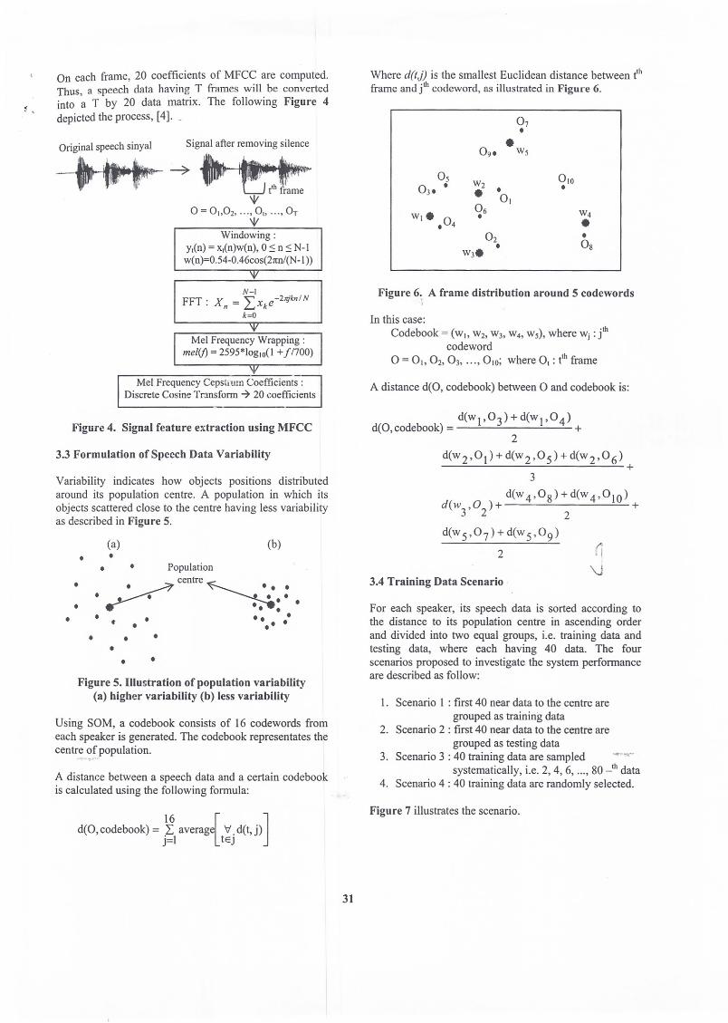
Where d(tj) is the smallest Euclidean distance between t'hframe and j,h codeword, as illustrated in Figure 6.

07,e

09, Ws

OS W2 01003,, ,

e,0,

w,e06 W4

,04,

eO2

,, 08W3e

Figure 6: A frame distribution around 5 codewords,

In this case:Codebook = (WI, W2,W3,W4,ws), where Wj : j'h

codeword0= 0" O2, 03, ... ,010; where 0,: t'h frame

A distance d(O, codebook) between ° and codebook is:

d(wl ,°3) + d(wl,O 4)d(O, codebook) = +

2

d(w2,01) + d(w2,05) + d(w2,06)+

3

dew 4,°8) + dew 4,°10)d(w3'O)+ 2 +

dew 5,°7) + dew 5,°9)

2

3.4 Training Data Scenario

For each speaker, its speech data is sorted according tothe distance to its population centre in ascending orderand divided into two equal groups, i.e. training data andtesting data, where each having 40 data. The fourscenarios proposed to investigate the system performanceare described as follow:

I. Scenario I : first 40 near data to the centre aregrouped as training data

2. Scenario 2 : first 40 near data to the centre aregrouped as testing data

3. Scenario 3 : 40 training data are sampled "'fO,,-

systematically, i.e. 2, 4, 6, ... , 80 _'h data4. Scenario 4 : 40 training data are randomly selected.

Figure 7 illustrates the scenario.

31

Speaker:

r l .. !..!1. t!:!: I:••!..!!.:!:!.._~ ~ _

c.. .9 -,----"""-' -,,··c.=.-==·':T·::"=!~=!~"-'!!-=_...:.!-=J'-!. '-=~'-'~'"""r""'"L"'-"R -+--_....:!-" ..'-. ""..""h.=!!.!,,-,! ''T.:1,-,~=!-=!:!:= •• ::..:.'''''''--''--,.--'--

I .I~'.i7 -,-_--'."'-I'-."".I."'III."'II·TIr.=.~"".""1. .z: ,.-_

{j ..:.-"'.!!"'J,::.:i1=!!"'iii=!I!.""!•.:.,:._:..;_=-- _

L. a5 -.--_--'- ......••••!..•••••••:.".:z:"',t!!.!".'-",,!!.." .,..- __

2~ __ ~.=Ht~wr- ~_i.ii.li. I

.Il. .!.!!!n.!!.!!!!.

5 15 25distance from its codebook

Figure 7. Dotplot of 80 speech data for 10 speakers

4. Experiments and Results

A mixture Gaussian HMM with three components isdeveloped for each scenario with various numbers ofstates, i.e. from 3 up to 7 states, and observed itsrecognition rate. The experimental results are presented inTable l.

Table 1 shows that HMM is able to recognize speakerwith unguided utterance at 98.4% rate on the average.HMM with 6 numbers of states resulted the bestrecognition rate as described in Figure 8.

0.99.,---------------------,~ 0.991-------------~ 0.98.j--------------C 0.98-j-------------

:E 0.98C 0.981-----·~ 0.98i:: 0.98~ 0.98

0.983 4 5 7

Number of State

Figure 8. A comparison of recognition rates forvarious numbers of states

Table 1. Recognition rate per speaker for variousnumbers of states for four scenarios (Sc.).

Numb er of State Ree.Se. 3 4 5 6 7 Rate

40 40 40 40 40 1.00040 39 39 40 40 0.99040 40 40 40 40 1.00040 40 40 40 40 1.000

I 38 37 38 38 37 0.94039 40 39 39 39 0.98040 40 40 40 40 1.00038 38 38 38 38 0.95039 40 39 37 39 0.97040 40 40 40 40 1.00039 39 40 40 40 0.99040 40 40 40 40 1.00036 37 36 36 36 0.90538 38 38 38 38 0.950

2 40 40 40 40 40 1.00040 40 40 40 40 1.00040 40 40 40 40 1.00037 36 37 37 36 0.91536 36 38 38 37 0.925(~39 39 39 39 40 0.98939 39 40 40 40 0.99040 40 40 40 40 1.00040 40 40 40 40 1.00040 40 39 39 39 0.985

3 38 38 38 38 38 0.95040 40 40 40 40 1.00040 40 40 40 40 1.00036 36 36 38 36 0.91039 40 38 39 37 0.96540 40 40 40 40 1.00040 40 40 40 40 1.00040 40 40 40 40 1.00040 40 40 40 40 1.00040 40 40 40 40 1.000

4 40 39 39 39 39 0.98040 40 40 40 40 1..00040 40 40 40 40 1.00039 39 39 39 39 0.97540 40 40 39 40 0.99539 39 39 39 40 0.980

Ree.~-~ '"

rate 0.9825 0.9831 0.9838 0.9850 0.9844 0.984

As expected from the scenario design, Scenario 2 yieldedthe worst recognition rate, i.e. 96.65% on the average asdepicted in Figure 9 and Figure 10.

32

Oseen -11 - ._-

• seen_2., - I---- - o seen_3•• 0.99

"' " I-rt -~-=r-~ I--- I-- Oseen 4c: 0.98 .' -----=-= -~'':: 0.97 , I-It 1- -~'a -\ l- I- I- ..,. 0.96 !'e<J

-~I--- 1- -<l., 0.95

"' "0.94

3 4 5 6 7

Number of State

Figure 9. A comparison of recognition rates forvarious numbers of states for each scenario

1.00.,---·-----------==-..fl 0.99~ 0.99+-------------c 0.98.S: 0.98:a 0.97eo 0.97eal 0.96

"' 0.960.95

4

Training Scenario

Figure 10. A comparison of recognition rates perscenario

These results indicate that if further objects were sampledfor training data then recognition rate will significantlydrop.

Distance from its Accuracy:. codebook Average Scenario 2

•• 11 •10 ..,---=-.""! .. .:..:!!..:.... "'-~!:"-'!:!."-='._=;·.!=!.:!=~!.==._:::.c=--.'='-_':'-'-'--_ 0.99 0.98

9

R +--""~=.._=_=' =..,.'=-=-=. 1=.••.=. ''-=--'-' -,--'-- 0.94••• 1 •• ,Jil.il;l.i.L •.••..7 1.00

! ::(j ...!!.!d j!!Hi!i. L,_- 1.00

i.. 1

5 .-_--'-...!--""""~""·:.,i ••"'·I'~!!.2I1'-',,,!!!..I1--___;-- 0.97

Speaker

..~ .. ! .. 0.96 0.93

0.921.00

1.00

1.00

4 -.-_,--,-,-, ...=d.f...,JIM=,i,,,,,,,,lll,,-,, ""------,r--- 0.98

3 --'---'-~='-=:=,=:r=--- ..:.....'__ -,_ 0.98

2 ,-_-=-. ~=:=.,Wr=--" ,--_ 1.00

0.95

0.91

1.00:

i.li. Ii I I

.- __ -'--",.=-" =j.:,!.::::!!::::!!.::::H.!::..:.! !.:!.t --'--_,- __ 1.00 0.995 15. 25

Figure 11. Recognition rate per speaker using Scenario 2

However, this scenario does not affect much HMMperformance to recognize the speaker, i.e. 96.65% is atolerable rate, due to variability in duration and pressure

has an ignorable effect. In other word, HMM is a robustmethod to overcome these variations .

Detailed observation in Scenario 2, indicates a multi-modals speech data distribution of a speaker has acontribution in lowering the system recognition rate(Speaker 3,8, and 9) as shown in Figure 11.

These findings predict that the system accuracy will dropfurther if speaker physical condition (healthiness, age, andemotion) is different. The prediction is most likelysupported by the fact that a speaker physical conditionwill affect on the voice distribution pattern.

5. Conclusion

Experimental results proved the robustness of HMMspeaker identification system for unguided utterance(duration and pressure) by resulting satisfactionrecognition rate (on the average, 96.65% up to 99.3%)using four different scenarios were applied.

The optimal number of states in the HMM is 6 with98.4% accuracy on the average. Furthermore, samplingtechnique in partitioning training and testing data alsoaffects the system accuracy. In this case, randomsampling gives the best result.

A multi-modals speech data of a speaker will significantlydrop the system recognition rate.

6. Future Research

Future research will focused in handling a multi-medalsspeech data of a speaker in noisy environment usingmodified HMM as classifier. Also, seeks an appropriatefeature extraction to handle the problems, i.e. multi-modals and noisy data.

References

[1] J. Campbell, "Speaker Recognition: A Tutorial", Proc. ofthe IEEE, Vol 85,No.9, 1997, 1437-1462.

[2] L.R. Rabiner, "A Tutorial on Hidden Markov Modelsand Selected Applications in Speech Recognition",Proceeding IEEE, Vol 77 No.2, 1989,257-289.

[3] Rakesh D. "A Tutorial on Hidden Markov Model.Technical Report, Departement of Electrical Engineering,Indian Institute of Technology, Bombay", 1996

[4] Todor D. Ganchev. Speaker Recognition. PhDDissertation, Wire Communications Laboratory,Department of Computer and Electrical Engineering,University of Patras Greece. 2005

33