A Fast Green Noise Digital Halftoning Algorithm with Section-oriented Multiscale Error Diffusion

Yik-Hing Fung and Yuk-Hee Chan

Center for Multimedia Signal Processing

Department of Electronic and Information Engineering, The Hong Kong Polytechnic University, Hong Kong Email: yhfung@eie.polyu.edu.hk , enyhchan@polyu.edu.hk

Abstract - Printing systems with poor and unstable dot gain make blue noise halftoning inappropriate to be used to generate halftone outputs for them, and green noise halftoning is preferred in such a case. Recently, a green noise halftoning with multiscale error diffusion (FMEDg) is proposed for this scenario. Extensive analysis and simulation results show that it can provide better halftoning performance in terms of various measures. In this paper, a section-oriented MED algorithm is proposed to reduce the computational effort of FMEDg. Simulation results show that the proposed fast algorithm can reduce the computational effort significantly and produce halftones of quality close to FMEDg.

I. I

Digital halftoning is a technique used to turn a gray-level image into a bi-level image and has been widely used in printing applications [1-3]. In practice, the size and the shape of a printed dot are not as perfect as they are expected. As a result, there is generally an increase in the size of a printed dot with respect to its ideal dot size. Such a phenomenon is called dot gain effect. When the size and shape are stable from dot to dot, a dot gain compensation technique can be used to minimize this distortion. However, when this is not the case, dot gain compensation does not work properly and green noise halftoning [4-7] is preferred to blue noise halftoning. A green noise halftoning output contains only mid-frequency spectral components and was proven to be less susceptible to image degradation from nonideal printing devices.

Recently, Fung and Chan [6] proposed a multiscale error diffusion algorithm called FMEDg for green noise digital halftoning. Analysis and simulation results show that it provides better performance in terms of various measures as compared with conventional green noise halftoning algorithms. However, due to its frame-oriented nature, its computation complexity is high when it is realized in a straight forward manner. In this paper, a fast multiscale error diffusion algorithm for green noise digital halftoning is proposed. The proposed algorithm is section-oriented rather than frame-oriented and hence able to significantly reduce the computational effort as compared with FMEDg.

The organization of this paper is as follows. In section II, the proposed section-oriented multiscale error diffusion for green noise halftoning is presented. In Section III, an analysis on the computational complexity of the proposed algorithm is given. In section IV, an empirical performance analysis based

on various statistics is provided to quantitatively evaluate the performance of the proposed algorithm. In section V, simulation results on real images are provided. Finally, a conclusion is given in Section VI.

ROPOSED

Without loss of generality, consider we want to halftone an input gray-level image X of size kk 22 × , where k is a positive integer, to obtain a binary output image B . The pixel values of X are within 0 and 1, where 0 and 1 represents the minimum and the maximum intensity values respectively.

At the very beginning, an error image E is constructed and initialized to be X to support the halftoning process. The proposed algorithm is section-oriented. In particular, the image is partitioned into a number of sections of size kh 2× each, where h is the height of the section, and sections are processed one by one downward. The appropriate number of white dots that should be assigned to a particular section is determined as the sum of the pixel values of X in the section. With this white dot budget on hand, pixels are located one by one using the maximum error intensity guidance rule until the white dot budget for the section is used up. Once a pixel is located in the section, a white dot is assigned to it and the corresponding quantization error of the pixel in the error image E is diffused to the pixel’s not-yet-processed neighboring pixels.

In the previous discussion, we assign white dots to a section. It is because we assume that white dots are the minority dots in the section. In practice, whether white dots or black dots are assigned to a section depends on the total energy of the section. If the average energy of a pixel in the section is larger than 0.5, black dots should be assigned instead to reduce the number of pixels needed to be located so as to reduce the realization effort further. This can be easily achieved with a simple trick. In particular, when black dots are needed to be assigned to a section, one can complement the corresponding section and its following section of the error image E before the section is processed, and complementing them again after it is processed. The complementing process is realized by jiji ee ,, 1: −= , where := is the assignment operator

and jie , is the (i,j)th element (i.e. the element at row i and column j) of E , for all (i,j) belonging to the involved sections. By doing this and complementing the corresponding section of

NTRODUCTION

II. P ALGORITHM

APSIPA ASC 2011 Xi’an

the binary output image B , black dots are actually assigned though apparently we assign white dots to the section as before. Accordingly, in the following discussion, we will only address how white dots are assigned to a section.

Assigning dots to a section is realized with a two-step iterative algorithm. In step 1 of the iteration, the desirable location in the section for putting a new white dot (value=1) is determined using the so-called “maximum error intensity guidance” scheme. It starts with the corresponding section in the error image E as the region of interest. The region of interest is divided into four non-overlapped subregions of equal width. Any two adjacent subregions are combined to form a candidate region. From the three candidate regions formed, the one with the largest sum of all its elements is selected to be the new region of interest. Whenever there are more than one regions containing the same maximum value of sum, one of them is randomly selected. This step is repeated until a region of size 1×h is reached. The location of the pixel which possesses the maximum jie , value among the h pixels in the region is the selected location to put a white dot.

Let ),( qp be the pixel location selected in step 1. In step 2 of the iteration, a white dot is assigned to the binary output image B by making 1, =qpb , where qpb , denotes pixel

),( qp of B . The difference between the original error qpe ,

and the assigned output value qpb , is treated as a quantization

error, and it is diffused in the error image E to pixel qpe , ’s neighboring pixels with a rectified diffusion filter.

The unrectified diffusion filter, denoted as oRRF ),( 21

, is an

approximated ring filter whose ),( nm th filter coefficient is defined as

π)(),,(),,(

),(21

22

12

RRRnmARnmA

nmf o

−

−= (1),

where ),,( tRnmA for }2,1{=t is the common area of circle

tRyx ≤+ 22 and the square bounded by ≤<− xn 5.0 5.0+n and 5.05.0 +≤<− mym . The detail of its derivation

can be found in [6].

This filter is rectified to diffuse the quantization error at pixel ),( qp . In error diffusion, the error image E is updated as (2), shown at the bottom of the page, where Γ is the filter support of o

RRF ),( 21,

⎩⎨⎧ <

= else1

0 ,,

piorvalueaassignedbeenhasbifd ji

ji (3)

and

∑Γ∈−−

⋅−−=),(

,),(qjpi

jio dqjpifs (4)

White dots are iteratively assigned to the section until all the white dot budget for the section is used up. The pixels left behind in the section are assigned black dots and the residual error in the section is flushed downward to the next section to be processed. Starting from the second top row in the current section to the first row of the section below, row by row we collect all the errors from the row above and redistribute them to the pixels in the row of interest as follows.

:1

1,13

1,, ∑

−=−−+=

iinlnlnl eee for all n (5),

where row l is the current row of interest and row l-1 is the row above row l.

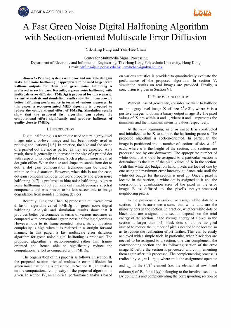
The processing of the current section is completed after flushing the residue error of the section, and then the next section will be processed. These steps are repeated until the whole image is processed. The flowchart shown in Fig. 1 summaries the steps of the proposed algorithm.

Fig. 1. Flowchart of the proposed algorithm

OMPUTATIONAL

In this section, a computational complexity analysis of the proposed algorithm is provided. The analysis is based on an assumption that the input image is of size NN × , where

⎩⎨⎧

Γ∈−−−⋅⋅−−−=

=),(/)(),(

),(),(0:

,,,,, qjpiifsebdqjpife

qpjiife

qpqpjio

jiji (2)

III. C C ANALYSIS OMPLEXITY

kN 2= and k is a positive integer.

The computational complexity of the proposed algorithm depends on (i) the size of the input image, (ii) the number of minority dots in a section, and (iii) the number of nonzero coefficients of the rectified diffusion filter used to diffuse the error of a pixel, which varies from pixel to pixel.

For each section, to ease the search of a desirable location to assign a white dot in the section, an energy tree is constructed at the beginning and then updated whenever a white dot is assigned to the section. Each tree node stores the sum of all jie , ’s in a predefined region. Assume that row L of the input image is the first row of a particular section. The value stored in the mth node at level l of the section’s energy tree is given as

∑ ∑−+

=

−+

==

1 1)1)(2/(

)2/( ,),(hL

Li

mN

mNj ji

l

l emlnode

for l=0,1… N2log and m=0,1,… l2 -1 (6)

The initialization of the energy trees for all sections takes around 2N additions in total.

In each iteration cycle, it takes around N2log2 comparisons and N2log additions to locate a pixel to assign

a white dot, which is around one seventh of that required in FMEDg. Diffusing the selected pixel’s error to its neighbors takes around P multiplications and P additions, where P is the number of non-zero coefficients of the rectified diffusion filter for the selected pixel. Note that the value of P depends on how many neighboring pixels of the selected pixel have already assigned white dots. It varies from location to location and is bounded by ⎡ ⎤ ⎡ ⎤112 22 +×+ RR . In general, the effort is only a half of that required in FMEDg. After diffusing the error, the energy tree of the section needs to be updated and it

takes around ⎡ ⎤ ⎡ ⎤∑ −

=− ++

1log

1 22 )12(2

N

ll RP additions.

Table 1 shows the execution time of Matlab realizations of FMEDg and the proposed algorithm used for halftoning the 256×256 8-bit gray-level testing images shown in Fig. 2. In our realization of the algorithms, we have 1R =1.8 and

12 2RR = . The section height used in the proposed algorithm is selected to be 1Rh = . The simulations were carried out on a 2.83 GHz Intel CoreTM 2 PC with 3.25 GB RAM. We can see from Table 1 that the proposed algorithm can significantly reduce the computational complexity as compared with FMEDg. Note that the realizations are straight-forward Matlab implementation without any optimization. An optimized C realization can effectively reduce the execution time. The figures shown in Table 1 are for comparison only.

1R =1.8, Image of size=256×256 Time (sec) Testing

Image FMEDg Proposed % of time

saved Barbara 165.13 5.781 96.499 Boat 226.75 6.625 97.078 House 117.63 5.485 95.337 Lena 219.11 6.016 97.254 Man 156.39 5.422 96.533 Peppers 154.64 5.078 96.716 Table 1. Execution time of the evaluated algorithms.

Fig. 2. Testing Images.

A

In this section, various spatial and spectral statistics were used to quantitatively evaluate the performance of the proposed algorithm. In our analysis, a set of constant gray-level images of size 256×256 were halftoned by the evaluated algorithm, and the dot distributions in its outputs were studied in terms of different statistics. Again, we have h= 1R =1.8 and

12 2RR = .

Spatial Statistics:

In [5], Lau developed a directional distribution function )(

21, αrrD to measure the directional distribution of dots in a dot pattern. It is defined as the expected number of dots per unit area in an angular segment of the ring bounded by inner radius 1r and outer radius 2r in the spatial domain. The annular ring is centered at the center pixel of a cluster and the angular segments are indexed by α which specifies a segment’s directional position with respect to the center. In an ideal case, we have 1)(

21, =αrrD for all α ’s, which indicates an isotropic distribution in the pattern.

Fig. 3 shows the halftone results of FMEDg and the proposed algorithm for some different gray levels, and Figs. 4 and 5, respectively, show their corresponding )(,0 αΔD and

)(, αλ Δ+Δ gD measures. Note that )(,0 αΔD and )(, αλ Δ+Δ g

D

report the intra- and inter-cluster dot distributions of a halftone respectively. We can see that the intra- and inter-cluster dot distributions of the proposed algorithm’s outputs are very close to those of the outputs of FMEDg. There is no overall

IV. E P NALYSIS MPIRICAL ERFORMANCE

directional bias as their plots are more or less radially symmetric.

To have a complete picture of the directional characteristics of the intra-cluster and inter-cluster dot distributions for all input gray levels, two directional index functions based on )(,0 αΔD and )(, αλ Δ+Δ g

D are respectively

defined in [6] as

∑=

Δ−=8

1

2,0 ))(1(

81)(α

αDgDIntra for 05.0 >≥ g (7)

and

∑=

Δ+Δ−=16

1

2, ))(1(

161)(

αλ α

gDgDInter for 05.0 >≥ g (8),

where g is the input gray level. Their plots for the outputs of FMEDg and the proposed algorithm are shown in Fig. 6.

In an ideal case, )(gDIntra and )(gDInter should be zero for all g because an isotropic distribution of dots makes

)(,0 αΔD and )(, αλ Δ+Δ gD =1 for all α . The larger the value

of )(gDIntra or )(gDInter , the more severely the distribution is directional for the specific halftoning output.

Spectral Statistics:

Radically averaged power spectrum density (RAPSD) and anisotropy are two measures proposed by Ulichney to analyze the spectral statistics of a halftone pattern [3]. Both of them are defined based on the power spectrum of a halftone pattern.

RAPSD is defined as the average power of the frequency components in an annular ring with center radius pf in the spectral domain as follows.

∑∈

=)(

)(ˆ))((

1)(pfRfp

p fPfRN

fP (9),

where )( pfR is an annular ring of width pΔ partitioned from

the spectral domain and ))(( pfRN is the number of

frequency components in )( pfR . )(ˆ fP is the estimated power spectrum of the halftone pattern and it is obtained by averaging the periodograms of a number of windowed segments of the halftone pattern. Fig. 7 shows the performance of various algorithms in terms of RAPSD. We can see that the proposed algorithm have green noise characteristics in terms of RAPSD.

Anisotropy is defined as

∑∈

−

−=

)(2

2

)(

))()(ˆ(1))((

1)(rfRf p

p

pp

fP

fPfPfRN

fA (10)

and it is used to measure the strength of directional artifact. Directional components are considered to be not noticeable by human eyes when )( pfA <0 dB happens for all pf [3]. Fig. 8 shows the performance of various algorithms in terms of anisotropy. We can see that the anisotropy of the proposed algorithm is well below 0 dB.

IMULATION

To study the performance of the evaluated algorithms in handling real images, some 8-bit gray-level testing images including six 512×512 natural images shown in Fig. 2 were used in our simulations. For reference purpose, the results of Damera-Venkata et. al.’s algorithm[7] are also provided for comparison.

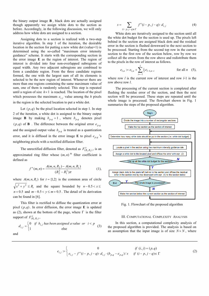
Fig. 9 shows portions of the original testing image “Barbara” and the corresponding outputs of the evaluated algorithms. We can see that the image quality of the proposed algorithm is close to FMEDg.

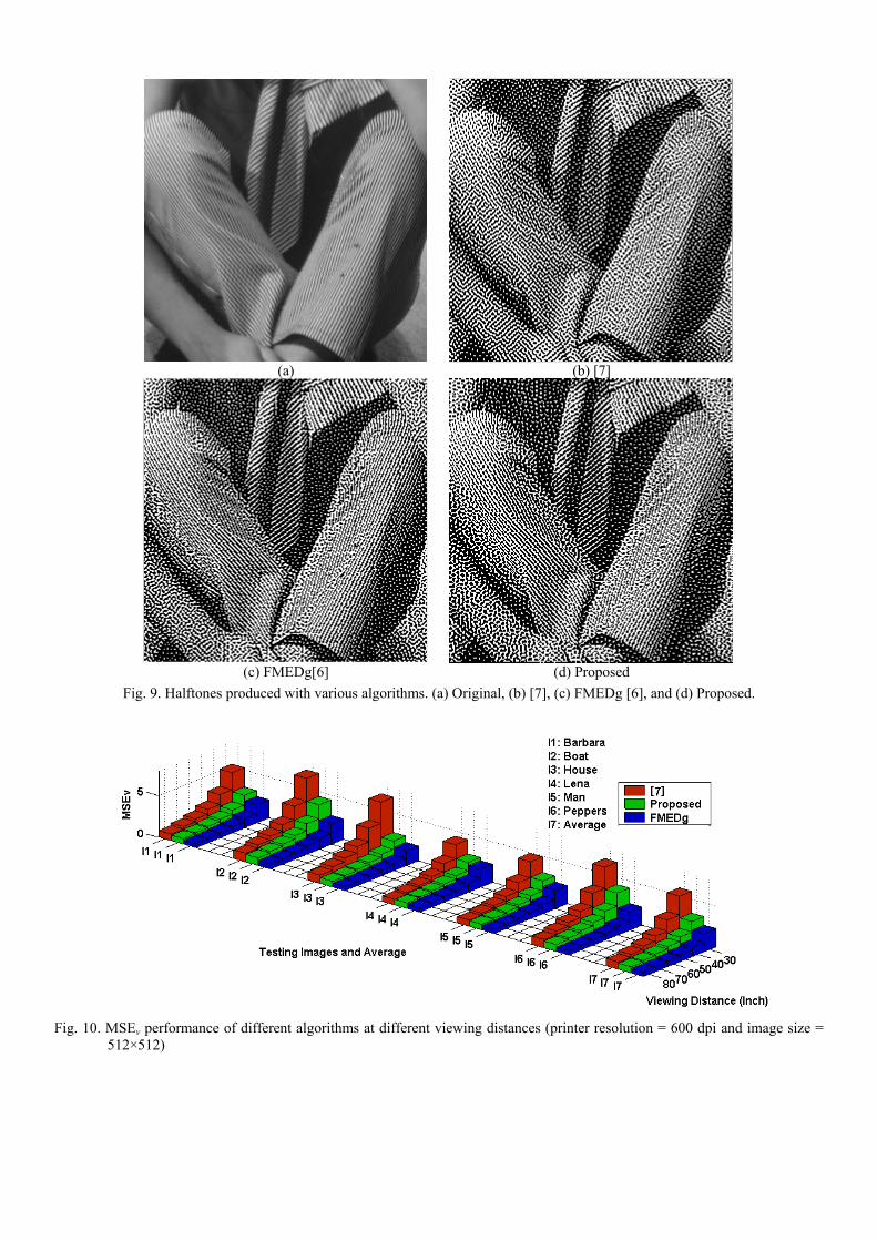
Fig. 10 shows the performance of FMEDg, Damera-Venkata et. al.’s algorithm[7] and the proposed algorithm in terms of vMSE . In particular, vMSE is defined as

NNdpivdBhvsdpivdXhvsv ×−= /),,(),,(MSE 2 (11)

where hvs is the HVS filter function defined in [2], vd is the viewing distance in inches and dpi is the printer resolution. In our simulations, the viewing distance changes from 30 to 80 inches and a printer resolution of 600 dpi was considered. We can see that the vMSE of the proposed algorithm is closer to FMEDg than Damera-Venkata et. al.’s algorithm[7].

ONCLUSIONS

In this paper, a fast green noise halfoning algorithm based on section-oriented multiscale error diffusion is proposed such that high quality halftone can be produced for printing systems having unstable dot gain. Simulation results show that the section-oriented nature of the proposed algorithm can significantly reduce the computational efforts while maintaining the halftone quality comparable to frame-oriented MED-based green noise halftoning algorithm.

CKNOWLEDGEMENT

This work was supported by Center for Multimedia Signal Processing and a grant from The Hong Kong Polytechnic University (PolyU Grant G-U865).

EFERENCES

1. R. A. Ulichney, Digital Halftoning. Cambridge, MA:MIT Press, 1987.

2. D. L. Lau and G. R. Arce, Modern Digital Halftoning, CRC Press 2nd edition 2008.

3. R. A. Ulichney, “Dithering with blue noise,” Proceedings of the IEEE, Vol. 76, pp. 56–79, Jan. 1988.

V. S RESULTS

VI. C

A

R

4. R. Levien, “Output dependent feedback in error diffusion halftoning,” IS&T Imaging Science and Technology 1, pp. 115-118, May 1993.

5. D. L. Lau, G. R. Arce, and N. C. Gallagher, “Green noise digital halftoning,” Proceedings of the IEEE, Vol. 86, pp. 2424-2442, Dec. 1998

6. Y.H. Fung and Y.H. Chan, “Green Noise Digital Halftoning with Multiscale Error Diffusion,” IEEE

Transaction on Image Processing, Vol.19, No.7, July 2010.

7. N. Damera-Venkata and B. L. Evans, “Adaptive threshold modulation for error diffusion halftoning,” IEEE Transaction on Image Processing, Vol. 10, No. 1, pp. 104–116, Jan. 2001.

(a) (b) (c) (d)

(i)

(ii)

Fig. 3. Parts of the halftoning results of 256×256 constant gray-level inputs obtained with (i) FMEDg, and (ii) the proposed algorithm. The input gray level is (a) g=33/255, (b) g=60/255, (c) g=82/255, and (d) g=116/255.

(i)

(ii)

Fig. 4. Corresponding directional distribution )(,0 αΔD plots of Fig. 3.

(i)

(ii)

Fig. 5. Corresponding directional distribution )(, αλ Δ+Δ gD plots of Fig. 3.

(a) (b) Fig. 6. (a) Intra- and (b) Inter-cluster distribution performance.

(a) (b) Fig. 7. Performance in terms of RAPSD: (a) FMEDg [6] and (b) proposed.

(a) (b) Fig. 8. Performance in terms of anisotropy: (a) FMEDg [6] and (b) proposed.

(a) (b) [7]

(c) FMEDg[6] (d) Proposed Fig. 9. Halftones produced with various algorithms. (a) Original, (b) [7], (c) FMEDg [6], and (d) Proposed.

Fig. 10. MSEv performance of different algorithms at different viewing distances (printer resolution = 600 dpi and image size =

512×512)