apuntes series de fourier
DESCRIPTION
Apuntes sobre series de Fourier Ramo Redes II UTFSMTRANSCRIPT

Signals and Systems with MATLAB Computing and Simulink Modeling, Fourth Edition 7 1
Copyright © Orchard Publications
Chapter 7
Fourier Series
his chapter is an introduction to Fourier series. We begin with the definition of sinusoidsthat are harmonically related and the procedure for determining the coefficients of the trig-onometric form of the series. Then, we discuss the different types of symmetry and how
they can be used to predict the terms that may be present. Several examples are presented toillustrate the approach. The alternate trigonometric and the exponential forms are also pre-sented.
7.1 Wave Analysis
The French mathematician Fourier found that any periodic waveform, that is, a waveform thatrepeats itself after some time, can be expressed as a series of harmonically related sinusoids, i.e.,sinusoids whose frequencies are multiples of a fundamental frequency (or first harmonic). For
example, a series of sinusoids with frequencies , , , and so on, contains the
fundamental frequency of , a second harmonic of , a third harmonic of ,
and so on. In general, any periodic waveform can be expressed as
or
where the first term is a constant, and represents the (average) component of .
Thus, if represents some voltage , or current , the term is the average value of
or .
The terms with the coefficients and together, represent the fundamental frequency compo-
nent * Likewise, the terms with the coefficients and together, represent the second har-
monic component and so on.
Since any periodic waveform ) can be expressed as a Fourier series, it follows that the sum of
* We recall that where is a constant.
T
� � � � � � � � � � � �� � � � � � � � � � � �� �� � ��� �� � �� � � � �� � � � � � � �� ��� �� � � �� � � � �� � � � � � �� � � � � � � � � � �� � ��� � �� � �� � ��� �� � � �� � � � � �� � ��� ���� � � � � � �� � � � � � � �� � � � � � � � � � � !" # $ � !$ % &' ! '" # $(
� � �

Chapter 7 Fourier Series
7 2 Signals and Systems with MATLAB Computing and Simulink Modeling, Fourth Edition
Copyright © Orchard Publications
the , the fundamental, the second harmonic, and so on, must produce the waveform .
Generally, the sum of two or more sinusoids of different frequencies produce a waveform that isnot a sinusoid as shown in Figure 7.1.
Figure 7.1. Summation of a fundamental, second and third harmonic
7.2 Evaluation of the Coefficients
Evaluations of and coefficients of (7.1) is not a difficult task because the sine and cosine are
orthogonal functions, that is, the product of the sine and cosine functions under the integral eval-
uated from to is zero. This will be shown shortly.
Let us consider the functions and where and are any integers. Then,
The integrals of (7.3) and (7.4) are zero since the net area over the to area is zero. The
integral of (7.5) is also is zero since
This is also obvious from the plot of Figure 7.2, where we observe that the net shaded area aboveand below the time axis is zero.
� � � �) * + , -. / 0 1 , 2 3 0 + , -4 0 1 5 , 6 2 * 0 7 89 6 1 5 , 6 2 * 0 7 8
: � : ; �; �� � � �<� = >�;� � � �<� = >�; �� � � � �� �� = �< >�? @� �� � � ��� �� ? @�� � � ? @A� � ���

Signals and Systems with MATLAB Computing and Simulink Modeling, Fourth Edition 7 3
Copyright © Orchard Publications
Evaluation of the Coefficients
Figure 7.2. Graphical proof of
Moreover, if and are different integers, then,
since
The integral of (7.6) can also be confirmed graphically as shown in Figure 7.3, where and
. We observe that the net shaded area above and below the time axis is zero.
Figure 7.3. Graphical proof of for and
Also, if and are different integers, then,
BC 7 0 B8 * CBC 7 0 B8 * C; �� � � � �� ��= �< >�
; �� � � � �� � � �<� = >�?� � � @� � � ��� �� ? @A� � ? @A� �A�4 BC 7 0 9 BC 7 0 4 BC 7 0 9 BC 7 0
; �� � � � �� � � �<� = >� ; �� � ��

Chapter 7 Fourier Series
7 4 Signals and Systems with MATLAB Computing and Simulink Modeling, Fourth Edition
Copyright © Orchard Publications
since
The integral of (7.7) can also be confirmed graphically as shown in Figure 7.4, where and
. We observe that the net shaded area above and below the time axis is zero.
Figure 7.4. Graphical proof of for and
However, if in (7.6) and (7.7), , then,
and
The integrals of (7.8) and (7.9) can also be seen to be true graphically with the plots of Figures7.5 and 7.6.
It was stated earlier that the sine and cosine functions are orthogonal to each other. The simpli-fication obtained by application of the orthogonality properties of the sine and cosine functions,becomes apparent in the discussion that follows.
In (7.1), Page 7 1, for simplicity, we let . Then,
;� � � � �� � �<� = >�?� � @� � ��� �� ? @�� � ? @A� ��� ; ��� �� 9 B8 * C 4 B8 * C 4 B8 * C 9 B8 * C;� � � � �� � �<� = >� ; �� � ��
; �� � � = �<� = �;� � � = �<� = ���� � ��� �� � �� � � � �� � � � � � � �� ��� �� � � �� � � � �� � � � � � �� � � � � � � � � � �� � ��� � �� � �

Signals and Systems with MATLAB Computing and Simulink Modeling, Fourth Edition 7 5
Copyright © Orchard Publications
Evaluation of the Coefficients
Figure 7.5. Graphical proof of
Figure 7.6. Graphical proof of
To evaluate any coefficient in (7.10), say , we multiply both sides of (7.10) by . Then,
Next, we multiply both sides of the above expression by , and we integrate over the period
to . Then,
BC 7 0 B=C 7 0; �� � � = �<� = �
B8 * C B=8 * C;� � � = �<� = �� �� � � �� � � ��� �� � �� � � � � � �� � �� � � � � � �� � �� � � � � � �� � � � � � � �� � �� ��� �� � � �� � � � � �� � �� � � � � � �� � � = � � � � � �� � � � � � � � �� � �� � ��� � �� � �
� � � �� � � �<� = ��� �� � �� � � �<� = � � � �� � �� � �<� = � � � � �� � �� � �<� =� �� � � � � � �� � �� � �<� = �� � � �� � � � �� � � �<� = � � � �� � � = �<� = � � � �� � � � �� � � � �<� =� �

Chapter 7 Fourier Series
7 6 Signals and Systems with MATLAB Computing and Simulink Modeling, Fourth Edition
Copyright © Orchard Publications
We observe that every term on the right side of (7.11) except the term
is zero as we found in (7.6) and (7.7). Therefore, (7.11) reduces to
or
and thus we can evaluate this integral for any given function . The remaining coefficients
can be evaluated similarly.
The coefficients , , and are found from the following relations.
The integral of (7.12) yields the average ( ) value of .
7.3 Symmetry in Trigonometric Fourier Series
With a few exceptions such as the waveform of the half rectified waveform, Page 7 17, the mostcommon waveforms that are used in science and engineering, do not have the average, cosine,and sine terms all present. Some waveforms have cosine terms only, while others have sine terms
only. Still other waveforms have or have not components. Fortunately, it is possible to pre-
dict which terms will be present in the trigonometric Fourier series, by observing whether or notthe given waveform possesses some kind of symmetry.
� � � �� � � � �<� =� � � �� � � �<� = � � � �� � � � �<� = � �� �� � �� � � � � � �� � � �<� =� � � � � � ��� �� ��� � � � � � � � �<� =� � �� � � � � � � �<� �� =�� � �� � � � � � � �<� � �� =�
� �

Signals and Systems with MATLAB Computing and Simulink Modeling, Fourth Edition 7 7
Copyright © Orchard Publications
Symmetry in Trigonometric Fourier Series
We will discuss three types of symmetry* that can be used to facilitate the computation of thetrigonometric Fourier series form. These are:
1. Odd symmetry If a waveform has odd symmetry, that is, if it is an odd function, the series will
consist of sine terms only. In other words, if is an odd function, all the
coefficients including , will be zero.
2. Even symmetry If a waveform has even symmetry, that is, if it is an even function, the series
will consist of cosine terms only, and may or may not be zero. In other
words, if is an even function, all the coefficients will be zero.
3. Half wave symmetry If a waveform has half wave symmetry (to be defined shortly), only odd(odd cosine and odd sine) harmonics will be present. In other words, alleven (even cosine and even sine) harmonics will be zero.
We defined odd and even functions in Chapter 6. We recall that odd functions are those forwhich
and even functions are those for which
Examples of odd and even functions were given in Chapter 6. Generally, an odd function has odd
powers of the independent variable , and an even function has even powers of the independent
variable . Thus, the product of two odd functions or the product of two even functions will
result in an even function, whereas the product of an odd function and an even function willresult in an odd function. However, the sum (or difference) of an odd and an even function willyield a function which is neither odd nor even.
To understand half wave symmetry, we recall that any periodic function with period , is
expressed as
that is, the function with value at any time , will have the same value again at a later time
.
A periodic waveform with period , has half wave symmetry if
* Quartet-wave symmetry is another type of symmetry where a digitally formed waveform with a series of zerosand ones contains only sine odd harmonics. We will not discuss this type of symmetry in this text. For a briefdiscussion, please refer to Introduction to Simulink with Engineering Applications, Page 7-18, ISBN 978-1-934404-09-6.
: :� �AA � ��� �A � ����
D� � � � D���A � D �� � ��

Chapter 7 Fourier Series
7 8 Signals and Systems with MATLAB Computing and Simulink Modeling, Fourth Edition
Copyright © Orchard Publications
that is, the shape of the negative half cycle of the waveform is the same as that of the positivehalf-cycle, but inverted.
We will test the most common waveforms for symmetry in Subsections 7.3.1 through 7.3.5below.
7.3.1 Symmetry in Square Waveform
For the waveform of Figure 7.7, the average value over one period is zero, and therefore,
. It is also an odd function and has half wave symmetry since and
.
Figure 7.7. Square waveform test for symmetry
An easy method to test for half wave symmetry is to choose any half period length on the
time axis as shown in Figure 7.7, and observe the values of at the left and right points on the
time axis, such as and . If there is half wave symmetry, these will always be equal but
will have opposite signs as we slide the half-period length to the left or to the right on the
time axis at non zero values of .
7.3.2 Symmetry in Square Waveform with Ordinate Axis Shifted
If in the square waveform of Figure 7.7 we shift the ordinate axis radians to the right, as
shown in Figure 7.8, we will observe that the square waveform now becomes an even function,
and has half wave symmetry since and . Also, .
Obviously, if the ordinate axis is shifted by any other value other than an odd multiple of ,
the waveform will have neither odd nor even symmetry.
D >� � �AA � ��� � D ��A � ��> E) +) F 4 ) F 4
GGH , H I
D �� �� � � D �� � �� �A � �� � � D ��A � �� >� �

Signals and Systems with MATLAB Computing and Simulink Modeling, Fourth Edition 7 9
Copyright © Orchard Publications
Symmetry in Trigonometric Fourier Series
Figure 7.8. Square waveform with ordinate shifted by
7.3.3 Symmetry in Sawtooth Waveform
For the sawtooth waveform of Figure 7.9, the average value over one period is zero and there-
fore, . It is also an odd function because , but has no half wave symmetry
since
Figure 7.9. Sawtooth waveform test for symmetry
7.3.4 Symmetry in Triangular Waveform
For this triangular waveform of Figure 7.10, the average value over one period is zero and
therefore, . It is also an odd function since . Moreover, it has half wave sym-
metry because .
Figure 7.10. Triangular waveform test for symmetry
J E)) F 4 ) F 4
GG � D � >� � �AA � ��� � D �� � �A
> 4)) F 4G
G ) F 4D >� � �AA � ��� � D �� � ��A
J 4) +G G) F 4 ) F 4

Chapter 7 Fourier Series
7 10 Signals and Systems with MATLAB Computing and Simulink Modeling, Fourth Edition
Copyright © Orchard Publications
7.3.5 Symmetry in Fundamental, Second, and Third Harmonics
Figure 7.11 shows a fundamental, second, and third harmonic of a typical sinewave.
Figure 7.11. Fundamental, second, and third harmonic test for symmetry
In Figure 7.11, the half period , is chosen as the half period of the period of the fundamental
frequency. This is necessary in order to test the fundamental, second, and third harmonics for
half wave symmetry. The fundamental has half wave symmetry since the and values,
when separated by , are equal and opposite. The second harmonic has no half wave symme-
try because the ordinates on the left and on the right, although are equal, there are not
opposite in sign. The third harmonic has half wave symmetry since the and values, when
separated by are equal and opposite. These waveforms can be either odd or even depending
on the position of the ordinate. Also, all three waveforms have zero average value unless theabscissa axis is shifted up or down.
In the expressions of the integrals in (7.12) through (7.14), Page 7 6, the limits of integration for
the coefficients and are given as to , that is, one period . Of course, we can choose
the limits of integration as to . Also, if the given waveform is an odd function, or an even
function, or has half wave symmetry, we can compute the non zero coefficients and by
integrating from to only, and multiply the integral by . Moreover, if the waveform has
half wave symmetry and is also an odd or an even function, we can choose the limits of integra-
tion from to and multiply the integral by . The proof is based on the fact that, the prod-
uct of two even functions is another even function, and also that the product of two odd func-tions results also in an even function. However, it is important to remember that when using
these shortcuts, we must evaluate the coefficients and for the integer values of that will
result in non zero coefficients. This point will be illustrated in Subsection 7.4.2, Page 7 14.
7.4 Trigonometric Form of Fourier Series for Common Waveforms
The trigonometric Fourier series of the most common periodic waveforms are derived in Subsec-tions 7.4.1 through 7.4.5 below.
a
a
b b
c
c
Fundamental Second harmonic Third harmonicD � AD � � � � �AD � � � � > � DA � � � �> �> � � � � � �

Signals and Systems with MATLAB Computing and Simulink Modeling, Fourth Edition 7 11
Copyright © Orchard Publications
Trigonometric Form of Fourier Series for Common Waveforms
7.4.1 Trigonometric Fourier Series for Square Waveform
For the square waveform of Figure 7.12, the trigonometric series consist of sine terms onlybecause, as we already know from Page 7 8, this waveform is an odd function. Moreover, onlyodd harmonics will be present since this waveform has also half wave symmetry. However, we
will compute all coefficients to verify this. Also, for brevity, we will assume that
Figure 7.12. Square waveform as odd function
The coefficients are found from
and since is an integer (positive or negative) or zero, the terms inside the parentheses on the
second line of (7.19) are zero and therefore, all coefficients are zero, as expected since the
square waveform has odd symmetry. Also, by inspection, the average ( ) value is zero, but if
we attempt to verify this using (7.19), we will obtain the indeterminate form . To work
around this problem, we will evaluate directly from (7.12), Page 7 6. Thus,
The coefficients are found from (7.14), Page 7 6, that is,
For , (7.21) yields
��> �)G
G : � �� � � � � � �� � �<� = �� � � K � �� � �<� KA � �� � �<=� K�� � � � � � � �� � � � � �� � � =A� �� K�� � � � � � � >A � � �� � ��� � �A� � � K�� � � � � � � � � �� � �A� � ��� � : � � > > � �� � � K �<� KA �<=� K� � � � >A �A � >� � �� :� � �� � � � � � �� � � �<� = �� � � K � �� � � �<� KA � �� � � �<=� K�� � � � � � �� �A � � � �� � =�� �� K�� � � � � � �� �A � � � �� �A� �� � K�� � � � � � � � �� �A � �� ����� L � L ��

Chapter 7 Fourier Series
7 12 Signals and Systems with MATLAB Computing and Simulink Modeling, Fourth Edition
Copyright © Orchard Publications
as expected, since the square waveform has half wave symmetry.
For , (7.21) reduces to
and thus
and so on.
Therefore, the trigonometric Fourier series for the square waveform with odd symmetry is
It was stated above that, if the given waveform has half wave symmetry, and it is also an odd or
an even function, we can integrate from to , and multiply the integral by . This property
is verified with the following procedure.
Since the waveform is an odd function and has half wave symmetry, we are only concerned with
the odd coefficients. Then,
For , (7.23) becomes
as before, and thus the series is as we found earlier.
Next let us consider the square waveform of Figure 7.13 where the ordinate has been shifted to
the right by radians, and has become an even function. However, it still has half wave sym-
metry. Therefore, the trigonometric Fourier series will consist of odd cosine terms only.
� � K�� � � � � � � �A �� >� �� < <� � � K�� � � � � � � � �� � � K�� � � � � � �� �� � � K� � � � � � ��� � � K�� � � � � � ��� M � KN� � � � � � ��� � � K� � � � � � � � ��� �� � � �N� �� N �� � �� �� � ��� � � � K� � � � � � � ��� �� � �� � �� O P P�� �> � �� � � � � �� � � � � � �� � � �<� = � K�� � � � � � � �� �A � � = � K�� � � � � � � � �� � �� �A ��� � �� < <� � � � K�� � � � � � � >A �� � K�� � � � � � �� �
�

Signals and Systems with MATLAB Computing and Simulink Modeling, Fourth Edition 7 13
Copyright © Orchard Publications
Trigonometric Form of Fourier Series for Common Waveforms
Figure 7.13. Square waveform as even function
Since the waveform has half wave symmetry and is an even function, it will suffice to integrate
from to and multiply the integral by . The coefficients are found from
We observe that for , all coefficients are zero, and thus all even harmonics are zero
as expected. Also, by inspection, the average ( ) value is zero.
For , we observe from (7.25) that , will alternate between and depending
on the odd integer assigned to . Thus,
For , and so on, (7.26) becomes
and for , and so on, it becomes
Then, the trigonometric Fourier series for the square waveform with even symmetry is
The trigonometric series of (7.27) can also be derived as follows:
J 4)G
G> � � � � � �� � � � � � �� � �<� = �� � � K � �� � �<� = � K�� � � � � � � � �� � � � = � K�� � � � � � � � �� � �� � �� � � �� L � L �� � � �� < <� � �� � �� � � � � �A� � � K�� � � � � � ��� � N Q � �� � � K�� � � � � � ��� � R � � � N� � � KA �� � � � � � � � � ��
� � � K� � � � � � � � � � ��� ��A � � �N� �� N �� � A�� � � K� � � � � � � �A � �S=T T T T T T T T T T T T T T T T ��� �� �� � �� O P P�� �

Chapter 7 Fourier Series
7 14 Signals and Systems with MATLAB Computing and Simulink Modeling, Fourth Edition
Copyright © Orchard Publications
Since the waveform of Figure 7.12 is the same as that of Figure 7.13, but shifted to the right by
radians, we can use the relation (7.22), Page 7 12, i.e.,
and substitute with that is, we let With this substitution, relation
(7.28) becomes
and using the identities , , and so on, we rewrite
(7.29) as
and this is the same as (7.27).
Therefore, if we compute the trigonometric Fourier series with reference to one ordinate, andafterwards we want to recompute the series with reference to a different ordinate, we can use theabove procedure to save computation time.
7.4.2 Trigonometric Fourier Series for Sawtooth Waveform
The sawtooth waveform of Figure 7.14 is an odd function with no half wave symmetry; there-fore, it contains sine terms only with both odd and even harmonics. Accordingly, we only need
to find all coefficients.
Figure 7.14. Sawtooth waveform
By inspection, the component is zero. As before, we will assume that .
If we choose the limits of integration from to , we will need to perform two integrations
� � � � K� � � � � � � � ��� �� � � �N� �� N �� � �� �� � ��� � ��� � �� � ���� � K� � � � � � � �� � �� ��� �� � �� � �� �N� �� N �� � ��� � �� �� � ��� � �� � K� � � � � � � �� � �� ��� �� � � �� � � � � �� �N� �� N N �� � � � � ��� � �� �� � ��� � �� ? ��� � � ?� �� ? � ��� � � ?� �A�� � K� � � � � � � ��� �� � �N� �� N� � A�� �A� ��
� �> �DG
G� � ��> �

Signals and Systems with MATLAB Computing and Simulink Modeling, Fourth Edition 7 15
Copyright © Orchard Publications
Trigonometric Form of Fourier Series for Common Waveforms
since
However, we can choose the limits from to , and thus we will only need one integration
since
Better yet, since the waveform is an odd function, we can integrate from to and multiply the
integral by ; this is what we will do.
From tables of integrals,
Then,
We observe that:
1. If , and . Then, (7.32) reduces to
that is, the even harmonics have negative coefficients.
2. If , , . Then,
that is, the odd harmonics have positive coefficients.
Thus, the trigonometric Fourier series for the sawtooth waveform with odd symmetry is
� � K� � � � � > �K� � � � � � KA � �� A �� � K� � � � �� A � >� ? ? ?<� � � � =� � � � � � � � ? ? � ��A ?� ��� � �� � � K� � � � � � �� � � �<� � K =� � � � � � � � � �� � � �<� � K =� � � � � � � �� =� � � � � � �� � � ��� �� � �� �A �� � �� K� = =� � � � � � � � � � � � �� � � � � � �� �A � � K� = =� � � � � � � � � � � �� � � � �� �A��� L � L �� �� � � >� �� � ��� � � K� = =� � � � � � � � � � � �A � K�� � � � � � �A� �� < <� �� � � >� �� � �A� � � � K� = =� � � � � � � � � � � � � K�� � � � � � �� �� � � K� � � � � � � � ��� �� � � ��� �� � �� � � ��� �� � � �� � �A�� � �A� � � � K� � � � � � � �A � �S ��� �� � �� � �� �

Chapter 7 Fourier Series
7 16 Signals and Systems with MATLAB Computing and Simulink Modeling, Fourth Edition
Copyright © Orchard Publications
7.4.3 Trigonometric Fourier Series for Triangular Waveform
The sawtooth waveform of Figure 7.15 is an odd function with half wave symmetry; then, thetrigonometric Fourier series will contain sine terms only with odd harmonics. Accordingly, we
only need to evaluate the coefficients. We will choose the limits of integration from to
, and will multiply the integral by . As before, we will assume that .
Figure 7.15. Triangular waveform
By inspection, the component is zero. From tables of integrals,
Then,
We are only interested in the odd integers of , and we observe that:
For odd integers of , the sine term yields
Thus, the trigonometric Fourier series for the triangular waveform with odd symmetry is
� � >� � ��> 4) +GG� � ? ? ?<� � � � �� � � � � � � ? ? � ��A ?� ��� � �� � � � K� � � � � � � � � �� � � �<� = U K �� � � � � � � � � �� � � �<� = U K �� � � � � � � �� �� � � � � � �� � � ��� �� � �� �A � =� � �U K� � �� � � � � � � � � � � �� � � � � � �� �A � = U K� � �� � � � � � � � � � � �� � �� � � � �� � � � �� � �� �A�� � � �� � �� � >�� � �� � �� � � � � V � � N Q � W L � � � U K� = =� � � � � � � � � � ����A � V � � R � � � W L � � � U K� = =� � � � � � � � � � �A���
� � U K =� � � � � � � � � � � �Q� ��A � � �� N� � � � � � N �� � � �� Q� � � � �� R �� � � �A�� � � U K =� � � � � � � �A � �S=T T T T T T T T T T T T T T T T �� =� � � � � �� � � �� O P P�� �
Signals and Systems with MATLAB Computing and Simulink Modeling, Fourth Edition 7 17
Copyright © Orchard Publications
Trigonometric Form of Fourier Series for Common Waveforms
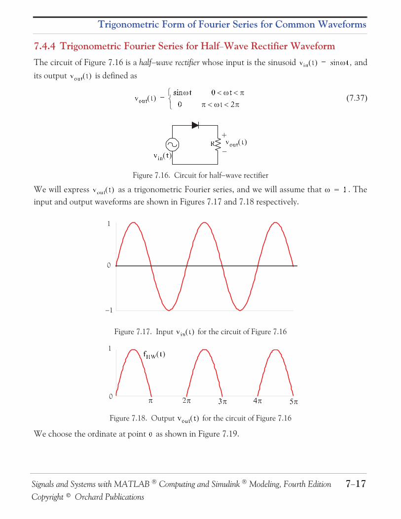
7.4.4 Trigonometric Fourier Series for Half Wave Rectifier Waveform
The circuit of Figure 7.16 is a half wave rectifier whose input is the sinusoid , and
its output is defined as
Figure 7.16. Circuit for half wave rectifier
We will express as a trigonometric Fourier series, and we will assume that . The
input and output waveforms are shown in Figures 7.17 and 7.18 respectively.
Figure 7.17. Input for the circuit of Figure 7.16
Figure 7.18. Output for the circuit of Figure 7.16
We choose the ordinate at point as shown in Figure 7.19.
� : � � �� � ��� O X Y � � O X Y � �� � � > �> � ��Z� : � � � O X Y �
� O X Y � ��1
1
0
� : � �� � � N
� [ \ �1
0 � O X Y �]

Chapter 7 Fourier Series
7 18 Signals and Systems with MATLAB Computing and Simulink Modeling, Fourth Edition
Copyright © Orchard Publications
Figure 7.19. Half wave rectifier waveform for the circuit of Figure 7.16
By inspection, the average is a non zero value, and the waveform has neither odd nor even sym-metry. Therefore, we expect all terms to be present.
The coefficients are found from
or
and from tables of integrals
Then,
Using the trigonometric identities
and
we obtain
and
Then, by substitution into (7.38),
A �> ��A � � �� � � � � � � �<� �� =� � K� � � � � � � �<� �� � �� K� � � � > � � �<� �=��; ?� � � � ?� � ?< ; �A ?� �� ; �A� � � � � � � � � � � � � � � � � � � � � � � � � � � � � �A ; �� ?� �� ; ��� � � � � � � � � � � � � � � � � � � � � � � � � � � � � � � ; = � =A� � K� � � � ��� �� � �A �� � � �A� � � � � � � � � � � � � � � � � � � � � � � � � � � � �� �� � � ��� � � � � � � � � � � � � � � � � � � � � � � � � � � �� �A� K�� � � � � �A �A� � � �A� � � � � � � � � � � � � � � � � � � � � � � � � � � � � ��� � � ��� � � � � � � � � � � � � � � � � � � � � � � � � � � � � �� �� �A� � � � � � � � � � �� �� ��� � � � � � � � � � � ��A� ? @A� � ? @� �� � ? � � � @� � ���? @�� � ? @ ? @� � �� � �A� �� ���A� � �� �� � �� � �� � �� �� �A� ���� � �� �� � �� � �� � �A �� �A� � � K�� � � � � �A �� �A � �A� � � � � � � � � � � � � � � � � � �� �A � ��� � � � � � � � � � � � � � � � � �� �� � �A� � � � � � � � � � � � � �A K�� � � � � � �� �� �A� � � � � � � � � � � � � � � �� �� ��� � � � � � � � � � � � � � �� �� � �A� � � � � � � � � � � � � ��� �

Signals and Systems with MATLAB Computing and Simulink Modeling, Fourth Edition 7 19
Copyright © Orchard Publications
Trigonometric Form of Fourier Series for Common Waveforms
or
Now, we can evaluate all the coefficients, except , from (7.39).
First, we will evaluate to obtain the value. By substitution of , we obtain
Therefore, the value is
We cannot use (7.39) to obtain the value of because this relation is not valid for ;
therefore, we will evaluate the integral
From tables of integrals,
and thus,
From (7.39) with , we obtain
We see that for odd integers of n, . However, for , we obtain
� K�� � � � � � � � � �� ��� ��� � � �� �A� � �A� � � � � � � � � � � � � � � � � � � � � � � � � � � � � � � � � � � � � � � � � � � � � � � � � � � � � � � � � � � � � � � � � � � � � � � � � � � � � � � � � � � � � � � �� � �A� � � � � � � � � � � � � �� K� � � � � ��� �� � �A� � � � � � � � � � � � � � � � � � � � � � � � � � �� � � � � � � >� � K�� � ��� �� K� � � �� � � �� � K� � � � � � �<� �� � ��� ?� � � ?� � ?< �� � � � � �� ?� � � =� � K�� � � � � � �� � � = � >� �� � � � N� � K� � � � � ��� �� � =A� � � � � � � � � � � � � � � � � � � � � � � � � � K�� � � � � � �A� � � K � ��� �� � =A� � � � � � � � � � � � � � � � � � � � � � � � � � � � � � � � � � >� � � >� � L � L �� � K � ��� �� � =A� � � � � � � � � � � � � � � � � � � � � � � � � � � � � � � � � � � K� N� � � � � � � � �A� � ^ K _ ��� �� _ =A� � � � � � � � � � � � � � � � � � � � � � � � � � � � � � � � � � � K� N� � � � � � � � �A� �

Chapter 7 Fourier Series
7 20 Signals and Systems with MATLAB Computing and Simulink Modeling, Fourth Edition
Copyright © Orchard Publications
and so on.
Next, we need to evaluate the coefficients. For this waveform,
and from tables of integrals,
Therefore,
that is, all the coefficients, except , are zero.
We will find by direct substitution into (7.14), Page 7 6, for . Thus,
Combining (7.40), with (7.42) through (7.47), we find that the trigonometric Fourier series forthe half wave rectifier with no symmetry is
7.4.5 Trigonometric Fourier Series for Full Wave Rectifier Waveform
Figure 7.20 shows a full wave rectifier circuit with input the sinusoid . The out-
put of that circuit is .
` K U ��� �� U =A� � � � � � � � � � � � � � � � � � � � � � � � � � � � � � � � � � � K_ �� � � � � � � � �A� �� �� � K �� � � � � � � �<� � �� = K� � � � � � � �<� � �� � �� K� � � � > � � �<� � �=�� �; ?� � � � ?� � � ?< ; �A ?� � �� ; �A� � � � � � � � � � � � � � � � � � � � � � � � � � � � � ; �� ?� � �� ; ��� � � � � � � � � � � � � � � � � � � � � � � � � � � � � � ; = � =A�� � K� � � � ��� �� � �A �� � � � �A� � � � � � � � � � � � � � � � � � � � � � � � � � � �� �� � � � ��� � � � � � � � � � � � � � � � � � � � � � � � � � �A �� K�� � � � � � � �A� � � � �A� � � � � � � � � � � � � � � � � � � � � � � � � � � � � ��� � � � ��� � � � � � � � � � � � � � � � � � � � � � � � � � � �A >A >� > � ���� � � �� � � ��� � K� � � � �� � � = �<� K� � � � ��� �� � �� � � �� � � � � � � � � � � �A � K� � � � �� � � �� � � �� � � � � � � � � � � � � �A K �� � � �� � � �� � K� � � � K �� � � � �� � � K� � � � � �� ��� � � � � � � � � � � � � � �� �� N� � � � � � � � � � � � � _ �� �� N� � � � � � � � � � � � � U �� �_ �� � � � � � � � � � � � �� � � �A��
� : � � K �� � ��� O X Y � K �� � ��

Signals and Systems with MATLAB Computing and Simulink Modeling, Fourth Edition 7 21
Copyright © Orchard Publications
Trigonometric Form of Fourier Series for Common Waveforms
Figure 7.20. Full-wave rectifier circuit
The input and output waveforms are shown in Figures 7.21 and 7.22 respectively. We will
express as a trigonometric Fourier series, and we will assume that .
Figure 7.21. Input sinusoid for the full rectifier circuit of Figure 7.20
Figure 7.22. Output waveform for full rectifier circuit of Figure 7.20
We choose the ordinate as shown in Figure 7.23.
Figure 7.23. Full wave rectified waveform with even symmetry
Z� : � � � O X Y �� O X Y � ��
A
A
0 � � �
a b c d e f a f baa g fa g ba g ha g ca g ia g da g ja g ea g kf >K � � �a b c d e f a f baa g fa g ba g ha g ca g ia g da g ja g ea g kf�A �A >
K

Chapter 7 Fourier Series
7 22 Signals and Systems with MATLAB Computing and Simulink Modeling, Fourth Edition
Copyright © Orchard Publications
By inspection, the average is a non zero value. We choose the period of the input sinusoid sothat the output will be expressed in terms of the fundamental frequency. We also choose the lim-
its of integration as and , we observe that the waveform has even symmetry. Therefore, we
expect only cosine terms to be present.
The coefficients are found from
where for this waveform,
and from tables of integrals,
Since
we express (7.49) as
To simplify the last expression in (7.50), we make use of the trigonometric identities
and
Then, (7.50) simplifies to
A � � � �� � � � � � � �<� �� =� � �� � � K � � � �<� �� � �S � K� � � � � � � � � � �<� �� � ����; ?� � � � ?� � ?< ; �A ?� �� � ;A� � � � � � � � � � � � � � � � � � � � � � � � � � � � � � ; �� ?� �� ; ��� � � � � � � � � � � � � � � � � � � � � � � � � � � � � � � ; = � =A�? @A� � @ ?A� � ? @� �� � ? � � � @� � ��� � � � K� � � � � � � ��� �� � �A �� � � �A� � � � � � � � � � � � � � � � � � � � � � � � � � � � �� �� � � ��� � � � � � � � � � � � � � � � � � � � � � � � � � � �A �� K� � � � � �A� � � �A� � � � � � � � � � � � � � � � � � � � � � � � � � � � � � ��� � � ��� � � � � � � � � � � � � � � � � � � � � � � � � � � � �A �� �A� � � � � � � � � � �� �� ��� � � � � � � � � � � �AA� K� � � � � � �� �A � ��� � � � � � � � � � � � � � � � � � � � � � � � � � � � � � � � � � � � � � � � A �A� � � �A� � � � � � � � � � � � � � � � � � � � � � � � � � � � � � � � � � � � � ��� � �� � � � �� � � � � �� � �A �� �A� �� A� � � � �� � � � � �� � �� �� �A� � � K� � � � � �� �� � ��� � � � � � � � � � � � � � � � � � � � � � � � � � �� �� � �A� � � � � � � � � � � � � � � � � � � � � � � ��A K� � � � �A � �A �� �� � �� �� �A� = �A� � � � � � � � � � � � � � � � � � � � � � � � � � � � � � � � � � � � � � � � � � � � � � � � � � � � � � � � � � � � � � � � � � � � � � � � � � � � � � � � � � � � �� �� KA � ��� �� = �A� � � � � � � � � � � � � � � � � � � � � � � � � � � � � � � � � � � � � � � � � � ��

Signals and Systems with MATLAB Computing and Simulink Modeling, Fourth Edition 7 23
Copyright © Orchard Publications
Trigonometric Form of Fourier Series for Common Waveforms
Now, we can evaluate all the coefficients, except , from (7.51). First, we will evaluate to
obtain the value. By substitution of , we obtain
Therefore, the value is
From (7.51) we observe that for all , other than , .
To obtain the value of , we must evaluate the integral
From tables of integrals,
and thus,
For , from (7.51) we obtain
and so on. Then, combining the terms of (7.52) with (7.54) through (7.57) we obtain
� � � � � >� � K� � � � � � ��� � ��� �� � K� � � � � � ��� < <� � �� � >� � � �� � � � � �<� �� � ��� ?� � � ?� � ?< �� � � � � �� ?� � � =� � ��� � � � � � �� � � = � >� �� L � L �� � � KA � ��� �� = �A� � � � � � � � � � � � � � � � � � � � � � � � � � � � � � � � � � � � � � � � � � K�� � � � � � �A� � � � KA � ��� �� = �A� � � � � � � � � � � � � � � � � � � � � � � � � � � � � � � � � � � � � � � � � � K� N� � � � � � � � �A� � ^ � KA _ ��� �_ = �A� � � � � � � � � � � � � � � � � � � � � � � � � � � � � � � � � � � � � � � � � � K� N� � � � � � � � �A� � ` � KA U ��� �U = �A� � � � � � � � � � � � � � � � � � � � � � � � � � � � � � � � � � � � � � � � � � K_ �� � � � � � � � �A� �� � � K� � � � � � � � K� � � � � � � � �� � �� � � � � � � � � � � � � � � � � � � �� � � N� � � � � � � � � � � � � � � � � � _ �� � � N� � � � � � � � � � � � � � � � � � U �� � _ �� � � � � � � � � � � � � � � � � �� � � �A�

Chapter 7 Fourier Series
7 24 Signals and Systems with MATLAB Computing and Simulink Modeling, Fourth Edition
Copyright © Orchard Publications
Therefore, the trigonometric form of the Fourier series for the full-wave rectifier with even symme-try is
This series of (7.59) shows that there is no component of the input (fundamental) frequency.
This is because we chose the period to be from and . Generally, the period is defined as
the shortest period of repetition. In any waveform where the period is chosen appropriately, it isvery unlikely that a Fourier series will consist of even harmonic terms only.
7.5 Gibbs Phenomenon
In Subsection 7.4.1, Page 7 12, we found that the trigonometric form of the Fourier series of thesquare waveform is
Figure 7.24 shows the first 11 harmonics and their sum. As we add more and more harmonics,the sum looks more and more like the square waveform. However, the crests do not become flat-tened; this is known as Gibbs phenomenon and it occurs because of the discontinuity of the per-
fect square waveform as it changes from to .
Figure 7.24. Gibbs phenomenon
7.6 Alternate Forms of the Trigonometric Fourier Series
We recall that the trigonometric Fourier series is expressed as
� � � K� � � � � � � � K� � � � � � � �� � �A� � � � � � � � � � � � � � � � � � � � �� �� = l m�A� A �� � � K� � � � � � � � ��� �� � � �N� �� N �� � �� �� � ��� � � � K� � � � � � � ��� �� � �� � �� O P P�� �
� K KA n o p q r s t u v v q w x p y z { p y z y |} ~ { z � � u o q r � � x � o { z y u � q
� � ��� �� � �� � � � �� � � � � � � �� ��� �� � � �� � � � �� � � � � � �� � � � � � � � � � �� � ��� � �� � �

Signals and Systems with MATLAB Computing and Simulink Modeling, Fourth Edition 7 25
Copyright © Orchard Publications
Alternate Forms of the Trigonometric Fourier Series
If a given waveform does not have any kind of symmetry, it may be advantageous of using thealternate form of the trigonometric Fourier series where the cosine and sine terms of the same fre-quency are grouped together, and the sum is combined to a single term, either cosine or sine.
However, we still need to compute the and coefficients separately.
For the derivation of the alternate forms, we will use the triangle shown in Figure 7.25.
Figure 7.25. Derivation of the alternate form of the trigonometric Fourier series
We assume and for , we rewrite (7.60) as
and, in general, for , we obtain
Similarly,
and, in general, where , we obtain
� � � � � �� �� � �� � � � � � � ��� � � � � � � � � � � � � � � � � � � � � � � �� �� � � � � �� �� � � � ��� �� � � � � ��� � � � � � � � � � � � � � � � � � � � � � �� �� � � � �� �� � � �� � � � � � � �� � �� �� � � � � � � ���� � �� � ���� � � � ��� � ��� �� � � �� �� � � � � � �� �� � � � � �� � ��� � � � �� �� � � � � � � �� �� � � � � � �� � ��� �� � �� � � � �� �� � � � � � � � �� �� � � � � � �� � ��� ���� �� � � � � � �� � �� � ��� �� � � �A� � � � � � � � � �� � �� � ��� �� � � � �A� �� � �� � � � � � � � � �� � �� � ��� �� � � � �A� ��� � ��� �� � � � � �A� �� ��� ��� �� � � � � � � �� � � � � � �A� �� ���� �� � ��� �� � � �� � � � �� � �� � ��� � � ��� � ��� � � �� � � � � �� � � �� � ��� � � � ��� � � � � �� � � � � �� � � �� � ��� � � � ��� � ����
Chapter 7 Fourier Series
7 26 Signals and Systems with MATLAB Computing and Simulink Modeling, Fourth Edition
Copyright © Orchard Publications
When used in circuit analysis, (7.61) and (7.62) can be expressed as phasors. Since it is custom-ary to use the cosine function in the time domain to phasor transformation, we choose to use thetransformation of (7.63) below.
Example 7.1
Find the first 5 terms of the alternate form of the trigonometric Fourier series for the waveform ofFigure 7.26.
Figure 7.26. Waveform for Example 7.1
Solution:
The given waveform has no symmetry; thus, we expect both cosine and sine functions with odd
and even terms present. Also, by inspection the value is not zero.
We will compute the and coefficients, the value, and we will combine them to obtain
an expression in the form of (7.63). Then,
We observe that for , .
For ,
� � ��� �� � � � � ��� � �� ��� ��� �� � � � � �� �� � � � � � ��� � �� ���� ���� �� � � � � � � �� � � � � � �A� �� ��� ��� �� � � � � �� � � � � � �A� ���
�4 94 +
� ���
� � � � � � � � �� � � � � �� � � �� � � � � �� � �<==�<� = ��� � � � � � � �� � � � = ��� � � � � � � �� � � ==�� ���� � � � � � � �� � �� � � ��� � � � � � � �� � � ��� � � � � � � �� � �� � �A� ��� � � � � � � �� � �� � ��� � L � L �� � >�� < <�

Signals and Systems with MATLAB Computing and Simulink Modeling, Fourth Edition 7 27
Copyright © Orchard Publications
Alternate Forms of the Trigonometric Fourier Series
and
The value is
The coefficients are
Then,
From (7.63),
where
Thus, for , we obtain:
Similarly,
� �� � �� � ��� � � � � �A�� � ��� �� ��� � � � � � � �<� = ��� � � � � � � �<==� ��� � � � � � � � � = � ==�� ���� � � � � � � �� � � � � � � �� � �A� ��� � � � � � �� ��� ��� ��� � � � �� � � � � �� � � � �� � � � � �� � � �<==�<� = �A�� � � � � � � �� � � = �A�� � � � � � � �� � ==�� ��A�� � � � � � � �� � �� � ��� � � � � � �A�� � � � � � � �� � ��� � � � � � � �� � �� �� � � ��� � � � � � � � �� �A ��� � � � � �� �� � � ��� � ��� � � ��� � � ����� �� � � � � � � �� � � � � � �A� �� ��� ��� � � � � � � �� � � � � � �A� ���� � � � �� � � � � � �A �= � �=� � � �� � � � � � �A �= � �=� �A � � � �A� � �� � � � � < �� � � � �A �� � � � �� � �A �� � � = �� � � =� � NA� �U =� � � � � � NA � �� � � � � � � � � � � NA � �� � � � � � � � � � � � NA� ���

Chapter 7 Fourier Series
7 28 Signals and Systems with MATLAB Computing and Simulink Modeling, Fourth Edition
Copyright © Orchard Publications
and
Combining the terms of (7.67) with (7.74) through (7.77), we find that the alternate form of thetrigonometric Fourier series representing the waveform of this example is
7.7 Circuit Analysis with Trigonometric Fourier Series
When the excitation of an electric circuit is a non sinusoidal waveform such as those we pre-sented thus far, we can use Fouries series to determine the response of a circuit. The procedure isillustrated with the examples that follow.
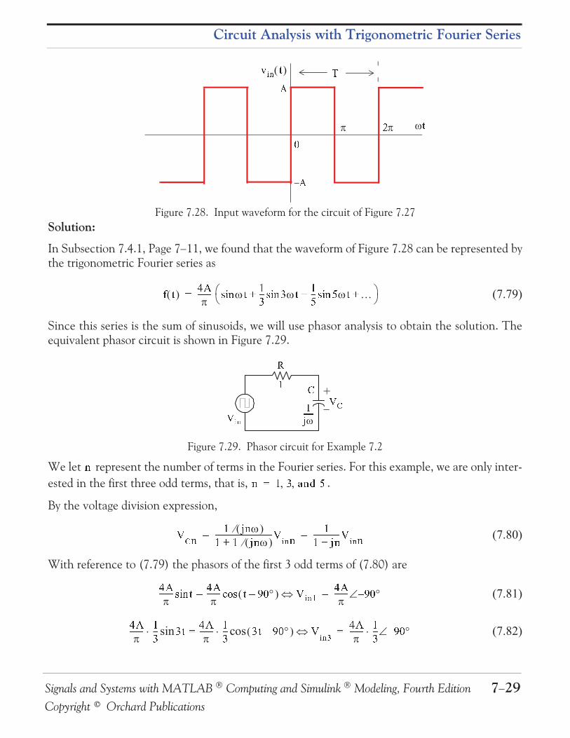
Example 7.2
The input to the series RC circuit of Figure 7.27, is the square waveform of Figure 7.28. Compute
the voltage across the capacitor. Consider only the first three terms of the series, and
assume .
Figure 7.27. Circuit for Example 7.2
� � � �A > � �� � �A �� � � Q >A� � �� � � � � Q >A� � � � � �A ��� � � � � �A � ��� � � � � �A � ��� � � � � � � � � � � � NA� � � ��� � � � � � � � � � � � � � NA� � � � � �A > � ��� � � � � �A ��� � � � � � Q >A� � ��� � � � � � � � Q >A� �� � ��� �� �� � � � � � � NA� � � � Q >A� ���� � � ��� � � � � � � � � � � � � � NA� � ��� �� � � Q >A� �� �
� � ��� �� : � � � � �� � ��
Signals and Systems with MATLAB Computing and Simulink Modeling, Fourth Edition 7 29
Copyright © Orchard Publications
Circuit Analysis with Trigonometric Fourier Series
Figure 7.28. Input waveform for the circuit of Figure 7.27
Solution:
In Subsection 7.4.1, Page 7 11, we found that the waveform of Figure 7.28 can be represented bythe trigonometric Fourier series as
Since this series is the sum of sinusoids, we will use phasor analysis to obtain the solution. Theequivalent phasor circuit is shown in Figure 7.29.
Figure 7.29. Phasor circuit for Example 7.2
We let represent the number of terms in the Fourier series. For this example, we are only inter-
ested in the first three odd terms, that is, .
By the voltage division expression,
With reference to (7.79) the phasors of the first 3 odd terms of (7.80) are
� �� ���
� : � �
� � � K� � � � � � � � ��� �� � � �N� �� N �� � �� �� � ��� � ��� �� � � �� � � � � � � � ��
� � � � � < N�� � � � � �� � � ��� � � � � � � � � � � � � � � � � � � � � � � � � � � � � � � : � � �� � ��� � � � � � � � � � � � � � � : � �� �� K� � � � � � � �� � � � K� � � � � � � � Q >A� �� � : � � � K� � � � � � � Q >A�� K� � � � � � � ��� �� � � � K� � � � � � � ��� �� � � Q >A� � : � � � K� � � � � � � ��� �� Q >A�

Chapter 7 Fourier Series
7 30 Signals and Systems with MATLAB Computing and Simulink Modeling, Fourth Edition
Copyright © Orchard Publications
By substitution of (7.81) through (7.83) into (7.80), we obtain the phasor and time domain volt-ages indicated in (7.84) through (7.86) below.
Thus, the capacitor voltage in the time domain is
Assuming that in the circuit of Figure 7.27 the capacitor is initially discharged, we expect thatcapacitor voltage will consist of alternating rising and decaying exponentials. Let us plot relation
(7.87) using the MATLAB script below assuming that .
Figure 7.30. Waveform for relation (7.87)
� K� � � � � � � �N� �� N � � K� � � � � � � �N� �� N � Q >A� � : � � � K� � � � � � � �N� �� Q >A�� � � �� ��� � � � � � � � � � � � K� � � � � � � Q >A �� � N� � � � � � � � � � � � � � � � � � � � � K� � � � � � � Q >A� �� K� � � � � � � ��� � � � � � � � � NA � K� � � � � � � ��� � � � � � � � � � NA�� � � �� � ��� � � � � � � � � � � � � � � K� � � � � � � ��� �� Q >A �� > R � � _� � � � � � � � � � � � � � � � � � � � � � � � � � � � � K� � � � � � � ��� �� Q >A� �� K� � � � � � � � >� >� � � � � � � � � � � _ � � _A � K� � � � � � � � >� >� � � � � � � � � � � � � _ � � _A�� � � �� � N�� � � � � � � � � � � � � � � K� � � � � � � �N� �� Q >A �� _ R U � R� � � � � � � � � � � � � � � � � � � � � � � � � � � � � K� � � � � � � �N� �� Q >A� �� K� � � � � � � � _� � >� � � � � � � � � � � _ U � RA � K� � � � � � � � _� � >� � � � � � � � � � N � � _ U � RA�
� � � � K� � � � � � � ��� � � � � � � � � � NA � >� >� � � � � � � � � � � � � _ � � _A � _� � >� � � � � � � � � � N � � _ U � RA� � �� K ��

Signals and Systems with MATLAB Computing and Simulink Modeling, Fourth Edition 7 31
Copyright © Orchard Publications
The Exponential Form of the Fourier Series
The waveform of Figure 7.30 is a rudimentary presentation of the capacitor voltage for the circuitof Figure 7.27. However, it will improve if we add a sufficient number of harmonics in (7.87).
We can obtain a more accurate waveform for the capacitor voltage of Figure 7.27 with the Sim-ulink model of Figure 7.31.
Figure 7.31. Simulink model for the circuit of Figure 7.27
The input and output waveforms are shown in Figure 7.32.
Figure 7.32. Input and output waveforms for the model of Figure 7.31
7.8 The Exponential Form of the Fourier Series
The Fourier series are often expressed in exponential form. The advantage of the exponential
form is that we only need to perform one integration rather than two, one for the , and
another for the coefficients in the trigonometric form of the series. Moreover, in most cases
the integration is simpler.
The exponential form is derived from the trigonometric form by substitution of
�� ��� � L � Y L � YS� �� � � � � � � � � � � � � � � � � � � � � � � � � � � ���� � � L � Y L � YSA� �� � � � � � � � � � � � � � � � � � � � � � � � � � ��

Chapter 7 Fourier Series
7 32 Signals and Systems with MATLAB Computing and Simulink Modeling, Fourth Edition
Copyright © Orchard Publications
into . Thus,
and grouping terms with same exponents, we obtain
The terms of (7.91) in parentheses are usually denoted as
Then, (7.91) is written as
We must remember that the coefficients, except , are complex and occur in complex con-
jugate pairs, that is,
We can derive a general expression for the complex coefficients , by multiplying both sides of
(7.95) by and integrating over one period, as we did in the derivation of the and
coefficients of the trigonometric form. Then, with ,
We observe that all the integrals on the right side of (7.96) are zero except the last. Therefore,
� � � � ��� �� � L � Y L � YS� �� � � � � � � � � � � � � � � � � � � � � � � � � � � � � L � = Y L � = YS� �� � � � � � � � � � � � � � � � � � � � � � � � � � � � � � � � �� � L � Y L � YSA� �� � � � � � � � � � � � � � � � � � � � � � � � � � � � � � L � = Y L � = YSA� �� � � � � � � � � � � � � � � � � � � � � � � � � � � � � � � �� � �� � ��� � ��� � � � � �� �� � � � �A L � = YS ��� � � � � �� �� � � � �A L � YS ��� �� ��� � � � � �� �� � � � �� L � Y ��� � � � � �� �� � � � �� L � = Y� � � � ��
� �S ��� �� � � ��� � � � �A ��� �� � � � ��� �� � ��� �� � � ��� � � � �� ��� �� � �A � �� �� ��� �� �� � � �� L � = YS � �� L � YS � � � L � Y � � L � = Y� � � � � �� � : � � �S � �� � �L � � YS � � ���� � L � � YS �<� = � =S L � = YS L � � YS �<� = � �S L � YS L � � YS �<� =� � � L � � YS �<� = � � L � Y L � � YS �<� =� � = L � = Y L � � YS �<� = � � L � � Y L � � YS �<� =� �� � ��
Signals and Systems with MATLAB Computing and Simulink Modeling, Fourth Edition 7 33
Copyright © Orchard Publications
Symmetry in Exponential Fourier Series
or
and, in general, for ,
or
We can derive the trigonometric Fourier series from the exponential series by addition and sub-
traction of the exponential form coefficients and . Thus, from (7.92) and (7.93),
or
Similarly,
or
7.9 Symmetry in Exponential Fourier Series
Since the coefficients of the Fourier series in exponential form appear as complex numbers, wecan use the properties in Subsections 7.9.1 through 7.9.5 below to determine the symmetry in theexponential Fourier series.
7.9.1 Even Functions
For even functions, all coefficients are real.
We recall from (7.92) and (7.93) that
� � L � � YS �<� = � � L � � Y L � � YS �<� = � � �<� = � � �� � �� � ��� � � � � � � � L � � YS �<� =�� � � ��� � � � � � � � L � � YS �<� =�� � �D� � � � � L � � YS �<� �� � � � �S� � � �S� ��� �� � � � �A � � � �� �� � � � � �S��� � � �SA ��� �� � � � �A �A �A � ��� � � � � � �SA�
� :� �S ��� �� � � ��� � � � �A ��� �� � � � ��� �

Chapter 7 Fourier Series
7 34 Signals and Systems with MATLAB Computing and Simulink Modeling, Fourth Edition
Copyright © Orchard Publications
and
Since even functions have no sine terms, the coefficients in (7.104) and (7.105) are zero.
Therefore, both and are real.
7.9.2 Odd Functions
For odd functions, all coefficients are imaginary.
Since odd functions have no cosine terms, the coefficients in (7.104) and (7.105) are zero.
Therefore, both and are imaginary.
7.9.3 Half Wave Symmetry
If there is half wave symmetry, for .
We recall from the trigonometric Fourier series that if there is half wave symmetry, all even har-
monics are zero. Therefore, in (7.104) and (7.105) the coefficients and are both zero for
, and thus, both and are also zero for .
7.9.4 No Symmetry
If there is no symmetry, is complex.
This is evident from Subparagraphs 7.9.1 and 7.9.2, and relations (7.104) and (7.105).
7.9.5 Relation of to
always.
This is evident from (7.104) and (7.105).
Example 7.3
Compute the exponential Fourier series for the square waveform of Figure 7.33 below. Assume
that .
� � ��� �� � � ��� � � � �� ��� � � � �A � �� � � �� �S � � � : �� �S � � � � >� � L � L �� � � �� L � L �� � �S � � � L � L ��� ��� �� � � �¡
¢¡
Signals and Systems with MATLAB Computing and Simulink Modeling, Fourth Edition 7 35
Copyright © Orchard Publications
Symmetry in Exponential Fourier Series
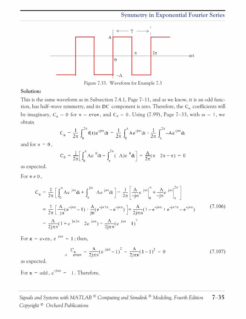
Figure 7.33. Waveform for Example 7.3
Solution:
This is the same waveform as in Subsection 7.4.1, Page 7 11, and as we know, it is an odd func-
tion, has half wave symmetry, and its component is zero. Therefore, the coefficients will
be imaginary, for , and . Using (7.99), Page 7 33, with we
obtain
and for ,
as expected.
For ,
For , ; then,
as expected.
For , . Therefore,
£ ¤¥¦¦ §
¨ � � �� � ©¡ ª « ¬ « ª¡ � ©¡ ¢¡� � ¢®̄ ¯ ¯ ¯ ¯ ¯ ° § « ± � ² §³´ µ ¢®̄ ¯ ¯ ¯ ¯ ¯ ¶ « ± � ² §³´ ¢®̄ ¯ ¯ ¯ ¯ ¯ ¶· « ± � ² §³µ¸¡ ¡ª ©¡ � ´ ¢®̄ ¯ ¯ ¯ ¯ ¯ ¶ « ´ §³´ ¶· « ´ §³µ¸ ¶®̄ ¯ ¯ ¯ ¯ ¯ ®· ¸ ©¡ ¡ ¡ª ©� � ¢®̄ ¯ ¯ ¯ ¯ ¯ ¶ « ± � ² §³´ ¶· « ± � ² §³µ¸ ¢®̄ ¯ ¯ ¯ ¯ ¯ ¶ ¹ ª·̄ ¯ ¯ ¯ ¯ ¯ ¯ ¯ « ± � ² ´ ¶· ¹ ª·̄ ¯ ¯ ¯ ¯ ¯ ¯ ¯ « ± � ² µ¸¡ ¡¢®̄ ¯ ¯ ¯ ¯ ¯ ¶ ¹ ª·̄ ¯ ¯ ¯ ¯ ¯ ¯ ¯ « ± � ¢· ¶¹ ª¯ ¯ ¯ ¯ ¯ « ± � µ « ± � ·¸ ¶® ¹ ª¯ ¯ ¯ ¯ ¯ ¯ ¯ ¯ ¯ ¯ ¯ ¯ ¢ « ± � · « ± � µ « ± � ·¸¡¡ ¶® ¹ ª¯ ¯ ¯ ¯ ¯ ¯ ¯ ¯ ¯ ¯ ¯ ¯ ¢ « ± � µ ® « ± � ·¸ ¶® ¹ ª¯ ¯ ¯ ¯ ¯ ¯ ¯ ¯ ¯ ¯ ¯ ¯ « ± � ¢· µ¡¡ª « ¬ « ª¡ « ± � ¢¡ � �º » ¼ » º½ ¶® ¹ ª¯ ¯ ¯ ¯ ¯ ¯ ¯ ¯ ¯ ¯ ¯ ¯ « ± � ¢· µ ¶® ¹ ª¯ ¯ ¯ ¯ ¯ ¯ ¯ ¯ ¯ ¯ ¯ ¯ ¢ ¢· µ ©¡ ¡ ¡ª ¾ ³ ³¡ « ± � ¢·¡
Chapter 7 Fourier Series
7 36 Signals and Systems with MATLAB Computing and Simulink Modeling, Fourth Edition
Copyright © Orchard Publications
Using (7.94), Page 7-32, that is,
we obtain the exponential Fourier series for the square waveform with odd symmetry as
The minus ( sign of the first two terms within the parentheses results from the fact that
. For instance, since , it follows that . We
observe that is purely imaginary, as expected, since the waveform is an odd function.
To prove that (7.109) above and (7.22), Page 7 12 are the same, we group the two terms inside
the parentheses of (7.109) for which ; this will produce the fundamental frequency .
Then, we group the two terms for which , and this will produce the third harmonic
, and so on.
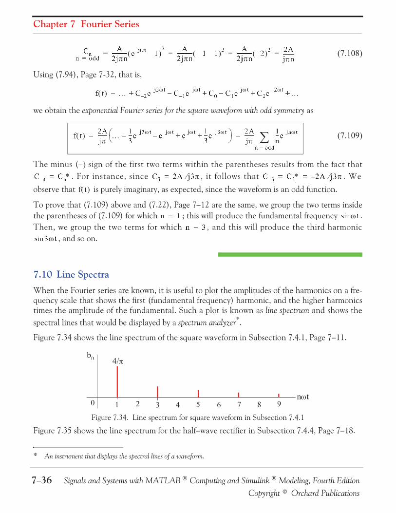
7.10 Line Spectra
When the Fourier series are known, it is useful to plot the amplitudes of the harmonics on a fre-quency scale that shows the first (fundamental frequency) harmonic, and the higher harmonicstimes the amplitude of the fundamental. Such a plot is known as line spectrum and shows the
spectral lines that would be displayed by a spectrum analyzer*.
Figure 7.34 shows the line spectrum of the square waveform in Subsection 7.4.1, Page 7 11.
Figure 7.34. Line spectrum for square waveform in Subsection 7.4.1
Figure 7.35 shows the line spectrum for the half wave rectifier in Subsection 7.4.4, Page 7 18.
* An instrument that displays the spectral lines of a waveform.
� �º ¿ À À½ ¶® ¹ ª¯ ¯ ¯ ¯ ¯ ¯ ¯ ¯ ¯ ¯ ¯ ¯ « ± � ¢· µ ¶® ¹ ª¯ ¯ ¯ ¯ ¯ ¯ ¯ ¯ ¯ ¯ ¯ ¯ ¢· ¢· µ ¶® ¹ ª¯ ¯ ¯ ¯ ¯ ¯ ¯ ¯ ¯ ¯ ¯ ¯ ®· µ ® ¶¹ ª¯ ¯ ¯ ¯ ¯ ¯ ¯ ¯¡ ¡ ¡ ¡° § � µ « ± µ ² � Á « ± ² � ´ � Á « ± ² � µ « ± µ ²¸ ¸ ¸ ¸ ¸ ¸¡° § ® ¶¹¯ ¯ ¯ ¯ ¯ ¯ ¯ ¢Â̄ ¯̄ « ± à ² · « ± ² · « ± ² ¢Â̄ ¯̄ « ± à ²¸ ¸ ® ¶¹¯ ¯ ¯ ¯ ¯ ¯ ¯ ¢ª̄ ¯̄ « ± � ²� Ä Å ÅÆ¡ ¡� � � �¡ � à ® ¶ ¹ ¡ � à � à ® ¶· ¹ ¡ ¡° § ª ¢¡ §Ç È ªª ¡ §Ç È ª
�

Signals and Systems with MATLAB Computing and Simulink Modeling, Fourth Edition 7 37
Copyright © Orchard Publications
Line Spectra
Figure 7.35. Line spectrum for half wave rectifier, Page 7 17
The line spectra of other waveforms can be easily constructed from the Fourier series.
Example 7.4
Compute the exponential Fourier series for the waveform of Figure 7.36, and plot its line spectra.
Assume .
Solution:
This recurrent rectangular pulse is used extensively in digital communications systems. To deter-mine how faithfully such pulses will be transmitted, it is necessary to know the frequency compo-nents.
Figure 7.36. Waveform for Example 7.4
As shown in Figure 7.36, the pulse duration is . Thus, the recurrence interval (period) , is
times the pulse duration. In other words, is the ratio of the pulse repetition time to the dura-
tion of each pulse. For this example, the components of the exponential Fourier series are foundfrom
The value of the average ( component) is found by letting . Then, from (7.110) we
obtain
or
¦ ¦¨ �
¢¡© ®
¥¦ ¥ É® Ê Ë ÊË Ë� � ¢®̄ ¯ ¯ ¯ ¯ ¯ ¶ « ± � ² §³ ¶®̄ ¯ ¯ ¯ ¯ ¯ « ± � ² §³Ì Ì¡ ¡¨ � ª ©¡� ¶®̄ ¯ ¯ ¯ ¯ ¯ § Ì Ì ¶®̄ ¯ ¯ ¯ ¯ ¯ ˯ ¯ ¯ ˯ ¯ ¯¸¡ ¡

Chapter 7 Fourier Series
7 38 Signals and Systems with MATLAB Computing and Simulink Modeling, Fourth Edition
Copyright © Orchard Publications
For the values for , integration of (7.110) yields
or
and thus,
The relation of (7.113) has the form, and the line spectra are shown in Figures 7.37
through 7.39, for , and respectively by using the MATLAB scripts below.
Figure 7.37. Line spectrum of (7.113) for
� ¶ ˯ ¯ ¯ ¯¡ª ©� � ¶¹ ª ®·̄ ¯ ¯ ¯ ¯ ¯ ¯ ¯ ¯ ¯ ¯ ¯ ¯ ¯ ¯ « ± � ² Ì Ì ¶ª̄ ¯ ¯ ¯ ¯ ¯ « ± � Ì « ± � Ì ·¹ ®¯ ¯ ¯ ¯ ¯ ¯ ¯ ¯ ¯ ¯ ¯ ¯ ¯ ¯ ¯ ¯ ¯ ¯ ¯ ¯ ¯ ¯ ¯ ¯ ¯ ¯ ¯ ¯ ¯ ¯ ¯ ¯ ¯ ¯ ¯ ¯ ¯ ¶ª̄ ¯ ¯ ¯ ¯ ¯ ª ˯ ¯ ¯ ¯ ¯ ¯Ç È ª ¶ ª ËÇ È ª ª¯ ¯ ¯ ¯ ¯ ¯ ¯ ¯ ¯ ¯ ¯ ¯ ¯ ¯ ¯ ¯ ¯ ¯ ¯ ¯ ¯ ¯ ¯ ¯ ¯ ¯¡ ¡ ¡ ¡� � ¶ ˯ ¯ ¯ ¯ ª ËÇ È ª ª ˯ ¯ ¯ ¯ ¯ ¯ ¯ ¯ ¯ ¯ ¯ ¯ ¯ ¯ ¯ ¯ ¯ ¯ ¯ ¯ ¯ ¯ ¯ ¯ ¯ ¯¡° § ¶ ˯ ¯ ¯ ¯ ª ËÇ È ª ª ˯ ¯ ¯ ¯ ¯ ¯ ¯ ¯ ¯ ¯ ¯ ¯ ¯ ¯ ¯ ¯ ¯ ¯ ¯ ¯ ¯ ¯ ¯ ¯ ¯ ¯� Æ¡ ÍÇ È ª ÍË ®¡ Ë Î¡ Ë ¢ ©¡
Ï Ð Ï Ñ Ï Ò Ï Ó Ô Ó Ò Ñ ÐÏ Ô Õ ÐÏ Ô Õ Ò ÔÔ Õ ÒÔ Õ ÐÔ Õ ÖÔ Õ ×ÓÓ Õ Ò Ø Ù Ò
Ë ®¡

Signals and Systems with MATLAB Computing and Simulink Modeling, Fourth Edition 7 39
Copyright © Orchard Publications
Line Spectra
Figure 7.38. Line spectrum of (7.113) for
Figure 7.39. Line spectrum of (7.113) for
The spectral lines are separated by the distance and thus, as becomes larger, the lines get
closer together while the lines are further apart as gets smaller.
Example 7.5
Use the result of Example 7.4 to compute the exponential Fourier series of the unit impulse train
shown in Figure 7.40.
Solution:
From relation (7.112), Page 7 38,
Ï Ð Ï Ñ Ï Ò Ï Ó Ô Ó Ò Ñ ÐÏ Ô Õ ÐÏ Ô Õ Ò ÔÔ Õ ÒÔ Õ ÐÔ Õ ÖÔ Õ ×ÓÓ Õ Ò Ø Ù Ú
Ë Î¡
Û Ü Û Ý Û Þ Û ß à ß Þ Ý ÜÛ à á ÜÛ à á Þ àà á Þà á Üà á âà á ãßß á Þ ä å ß à
Ë ¢ ©¡¢ Ë Ë˶ § ® ª

Chapter 7 Fourier Series
7 40 Signals and Systems with MATLAB Computing and Simulink Modeling, Fourth Edition
Copyright © Orchard Publications
Figure 7.40. Impulse train for Example 7.4
and the pulse width was defined as , that is,
Next, let us represent the impulse train of Figure 7.40, as a recurrent pulse with amplitude
as shown in Figure 7.41.
Figure 7.41. Recurrent pulse with amplitude
By substitution of (7.116) into (7.114), we obtain
and as , we observe from Figure 7.41, that each recurrent pulse becomes a unit impulse,
and the total number of the pulses reduce to a unit impulse train. Moreover, recalling that
, we see that (7.117) reduces to , that is, all coefficients of the exponential
Fourier series have the same amplitude and thus,
£ ¤ æ¦
ç è é¤é è ç � � ¶ ˯ ¯ ¯ ¯ ª ËÇ È ª ª ˯ ¯ ¯ ¯ ¯ ¯ ¯ ¯ ¯ ¯ ¯ ¯ ¯ ¯ ¯ ¯ ¯ ¯ ¯ ¯ ¯ ¯ ¯ ¯ ¯ ¯¡Ê Ë Ê̄ ¯ ¯ ®̄ ¯ ¯ ¯ ¯ ¯¡¶ ¢Ê̄ ¯ ¯ ¯ ¯ ¯ ¯ ¯ ¯ ¯ ¢®̄ ¯ ¯ ¯ ¯ ¯ ¯ ¯ ¯ ¯ ¯ ¯ ¯ ®̄ ¯ ¯ ¯ ¯ ¯¡ ¡ ¡
© ¤¥¦ ¤ ê¤
¦ ë¤ ìí í í í í í í í í í í í íî¦ ë¤ ìí í í í í í í í í í í í íî� � Ë ®Ë¯ ¯ ¯ ¯ ¯ ¯ ¯ ¯ ¯ ¯ ¯ ¯ ¯ ª ËÇ È ª ª ˯ ¯ ¯ ¯ ¯ ¯ ¯ ¯ ¯ ¯ ¯ ¯ ¯ ¯ ¯ ¯ ¯ ¯ ¯ ¯ ¯ ¯ ¯ ¯ ¯ ¯ ¢®̄ ¯ ¯ ¯ ¯ ¯ ª ËÇ È ª ª ˯ ¯ ¯ ¯ ¯ ¯ ¯ ¯ ¯ ¯ ¯ ¯ ¯ ¯ ¯ ¯ ¯ ¯ ¯ ¯ ¯ ¯ ¯ ¯ ¯ ¯¡ ¡Ë ©ÍÇ È ªÍ¯ ¯ ¯ ¯ ¯ ¯ ¯ ¯ ¯ ¯ï ´ð È ñ ¢¡ � � ¢®̄ ¯ ¯ ¯ ¯ ¯¡

Signals and Systems with MATLAB Computing and Simulink Modeling, Fourth Edition 7 41
Copyright © Orchard Publications
Computation of RMS Values from Fourier Series
The series of (7.118) reveals that the line spectrum of the impulse train of Figure 7.40, consists ofa train of equal amplitude, and are equally spaced harmonics as shown in Figure 7.42.
Figure 7.42. Line spectrum for Example 7.5
Since these spectral lines extend from , the bandwidth approaches infinity.
Let us reconsider the train of recurrent pulses shown in Figure 7.43.
Figure 7.43. Recurrent pulse with
Now, let us suppose that the pulses to the left and right of the pulse centered around zero,
become less and less frequent; or in other words, the period approaches infinity. In this case,
there is only one pulse left (the one centered around zero). As , the fundamental fre-
quency approaches zero, that is, as approaches infinity. Accordingly, the frequency dif-
ference between consecutive harmonics becomes smaller. In this case, the lines in the line spec-trum come closer together, and the line spectrum becomes a continuous spectrum. This formsthe basis of the Fourier transform that we will study in the next chapter.
7.11 Computation of RMS Values from Fourier Series
The value of a waveform consisting of sinusoids of different frequencies, is equal to the
square root of the sum of the squares of the values of each sinusoid. Thus, if
° § ¢®̄ ¯ ¯ ¯ ¯ ¯ « ± � ²� Æ¡
© ¢ ò®  ó¢ó  ®¢ ®
§ ¾· ¸© ¤
¥¦ ¥ ê¤ ¥ Ê Ê© Êô õ ö ô õ ö

Chapter 7 Fourier Series
7 42 Signals and Systems with MATLAB Computing and Simulink Modeling, Fourth Edition
Copyright © Orchard Publications
where represents a constant current, and represent the amplitudes of the sinuso-
ids, the value of is found from
or
The proof of (7.120) is based on Parseval’s theorem; we will state this theorem in the next chap-ter. A brief description of the proof of (7.120) follows.
We recall that the (effective) value of a function, such as current , is defined as
Substitution of (7.119) into (7.122), will produce the terms , , and other
similar terms representing higher order harmonics. The result will also contain products of cosinefunctions multiplied by a constant, or other cosine terms of different harmonic frequencies. Butas we know, from the orthogonality principle, the integration of (7.122), will produce all zeroterms except the cosine squared terms which, for each harmonic, will be
as in (7.121).
Example 7.6
Consider the waveform of Figure 7.44.
Figure 7.44. Waveform for Example 7.6
È ÷ ÷ ø ø § øù ¾ Ç ÷ ú ú § úù ¾ Ç ÷ û û § ûù ¾ Ǹ ¸ ¸ ¸¡÷ ÷ ø ÷ ú ÷ ûô õ ö È ÷ ü ý þ ÷ ú ÷ ø ü ý þú ÷ ú ü ý þú ÷ û ü ý þú¸ ¸ ¸ ¸¡÷ ü ý þ ÷ ú ¢®̄ ¯̄ ÷ ø ÿú ¢®̄ ¯̄ ÷ ú ÿú ¢®̄ ¯̄ ÷ û ÿú¸ ¸ ¸ ¸¡ô õ ö È §÷ � � � ¢Ê̄ ¯ ¯ È µ §³´ �¡ ÷ ú ÷ ø ÿú Á § Á·ù ¾ Ç ú
÷ � ú Ê ®¯ ¯ ¯Ê¯ ¯ ¯ ¯ ¯ ¯ ¯ ¯ ¯ ¢®̄ ¯̄ ÷ � ú¡ë
ë §
Signals and Systems with MATLAB Computing and Simulink Modeling, Fourth Edition 7 43
Copyright © Orchard Publications
Computation of RMS Values from Fourier Series
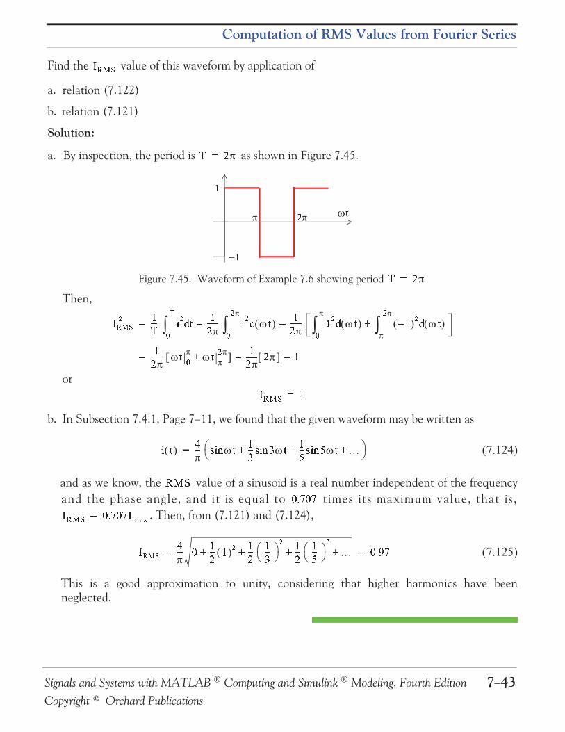
Find the value of this waveform by application of
a. relation (7.122)
b. relation (7.121)
Solution:
a. By inspection, the period is as shown in Figure 7.45.
Figure 7.45. Waveform of Example 7.6 showing period
Then,
or
b. In Subsection 7.4.1, Page 7 11, we found that the given waveform may be written as
and as we know, the value of a sinusoid is a real number independent of the frequency
and the phase angle, and it is equal to times its maximum value, that is,
. Then, from (7.121) and (7.124),
This is a good approximation to unity, considering that higher harmonics have beenneglected.
÷ � � �Ê ®¡ ë
ë §¤ Ê ®¡÷ ü ý þú ¢Ê̄ ¯ ¯ È ú §³´ � ¢®̄ ¯ ¯ ¯ ¯ ¯ È µ §³´ µ ¢®̄ ¯ ¯ ¯ ¯ ¯ ¢ ú §³´ ¢· ú §³µ¸¡ ¡¡ ¢®̄ ¯ ¯ ¯ ¯ ¯ § ´ § µ¸ ¢®̄ ¯ ¯ ¯ ¯ ¯ ® ¢¡ ¡¡ ÷ � � � ¢¡È § ó¯ ¯ ¯ §Ç È ª ¢Â̄ ¯̄  §Ç È ª ¢Î̄ ¯̄ Î §Ç È ª¸ ¸ ¸¡ô õ ö © � � © �÷ � � � © � � © � ÷ � � ï¡ ÷ ü ý þ ó¯ ¯ ¯ © ¢®̄ ¯̄ ¢ ú ¢®̄ ¯̄ ¢Â̄ ¯ ¯ ú ¢®̄ ¯̄ ¢Î̄ ¯̄ ú¸ ¸ ¸ ¸ © � � �¡ ¡
Chapter 7 Fourier Series
7 44 Signals and Systems with MATLAB Computing and Simulink Modeling, Fourth Edition
Copyright © Orchard Publications
7.12 Computation of Average Power from Fourier Series
We can compute the average power of a Fourier series from the relation
The proof is obtained from the definition of average power, i.e.,
and the expression for the alternate trigonometric Fourier series, that is,
where can represent voltages and currents. Then, by substitution of these series for and
into (7.127), we will find that the products of and that have different frequencies, will be
zero, and only the products of the same frequency terms will have non-zero values. The non zerovalues will represent the average power for each harmonic in (7.126).
Example 7.7
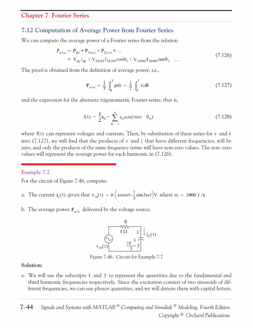
For the circuit of Figure 7.46, compute:
a. The current given that where .
b. The average power delivered by the voltage source.
Figure 7.46. Circuit for Example 7.7
Solution:
a. We will use the subscripts and to represent the quantities due to the fundamental and
third harmonic frequencies respectively. Since the excitation consists of two sinusoids of dif-ferent frequencies, we can use phasor quantities, and we will denote them with capital letters.
� � Å � Á � � µ � �¸ ¸ ¸¡ Å � ÷ Å � ø ü ý þ ÷ ø ü ý þ øù ¾ Ç ú ü ý þ ÷ ú ü ý þ úù ¾ Ǹ ¸ ¸¡ � � ¢Ê̄ ¯ ¯ � §³´ � ¢Ê̄ ¯ ¯ ¬ È §³´ �¡ ¡° § ¢®̄ ¯̄ � ´ ù � ª § �·ù ¾ Ç� ÁƸ¡° § ¬ Ȭ È
È � § ¬ � � § � § ¢Â̄ ¯̄  §ù ¾ Ç·ù ¾ Ç ¡ ¢ © © © � Ç¡ � � ë È � §¬ � � § ë £ ���í í í í í í í í í í í í �� �¢ Â

Signals and Systems with MATLAB Computing and Simulink Modeling, Fourth Edition 7 45
Copyright © Orchard Publications
Computation of Average Power from Fourier Series
Then,
Next,
From (7.129) and (7.130),
b. The average power delivered by the voltage source is
or
Check:
The average power absorbed by the capacitor is zero, and therefore, the average powerabsorbed by the resistor, must be equal to the average power delivered by the source. Theaverage power absorbed by the resistor is
¬ � � Á § � §ù ¾ Ç¡ � � Á � © ¡¹· Á �¯ ¯ ¯ ¯ ¯ ¯ ¯ ¯ ¯ ¯ ¹·¢ © à ¢ © à ¯ ¯ ¯ ¯ ¯ ¯ ¯ ¯ ¯ ¯ ¯ ¯ ¯ ¯ ¯ ¯ ¯ ¯ ¯ ¯ ¯ ¯ ¯ ¯ ¯ ¯ ¯ ¯ ¯ ¯ ¯ ¯ ¹ ·¡ ¡� Á ¢ ¹ · ¢ © � ¢ � �·¡ ¡÷ � Á � � Á� Á¯ ¯ ¯ ¯ ¯ ¯ ¯ ¯ ¯ ¯ � ©¢ © � ¢ � �·¯ ¯ ¯ ¯ ¯ ¯ ¯ ¯ ¯ ¯ ¯ ¯ ¯ ¯ ¯ ¯ ¯ ¯ ¯ ¯ ¯ ¯ ¯ ¯ ¯ ¯ ¯ ¯ ¯ ¯ ¯ ¢ � � © � ¢ � �¡ ¡ ¡ È � Á § ¢ � � © § � ¢ � �¸ ¶¡¬ � � à § ®·  §ù ¾ Ç ®  § ¢ � ©¸¡ ¡ � � à ® ¢ � © ¡¹· à �¯ ¯ ¯ ¯ ¯ ¯ ¯ ¯ ¯ ¯ ¹·Â ¢ © à ¢ © à ¯ ¯ ¯ ¯ ¯ ¯ ¯ ¯ ¯ ¯ ¯ ¯ ¯ ¯ ¯ ¯ ¯ ¯ ¯ ¯ ¯ ¯ ¯ ¯ ¯ ¯ ¯ ¯ ¯ ¯ ¯ ¯ ¯ ¯ ¯ ¯ ¯ ¯ ¯ ¯ ¯ ¹ ¢·¡ ¡� à ¢ ¹ ¢· ® ó η¡ ¡÷ � à � � Ã� ï ¯ ¯ ¯ ¯ ¯ ¯ ¯ ¯ ¯ ® ¢ � ©® ó η¯ ¯ ¯ ¯ ¯ ¯ ¯ ¯ ¯ ¯ ¯ ¯ ¯ ¯ ¯ ¯ ¯ ¯ ¯ ¯ ¯ ¯ ¯ ¯ ¢ � ó ¢ ® ® Î ¢ � ó ¢ ® ® Î ¢  η¡ ¡ ¡ ¡È � à § ¢ � ó ¢ Â § ¢  η ¶¡È � § È � Á § È � à §¸ ¢ � � © § � ¢ � �¸ ¢ � ó ¢ Â § ¢  η¸¡ ¡ � � ø ü ý þ ÷ ø ü ý þ øù ¾ Ç � ü ý þ ÷ � ü ý þ �ù ¾ Ǹ¡ � ®¯ ¯ ¯ ¯ ¯ ¯ ¯ ¢ � � ©®¯ ¯ ¯ ¯ ¯ ¯ ¯ ¯ ¯ ¯ � ¢ � � ® ®¯ ¯ ¯ ¯ ¯ ¯ ¯ ¢ � ó ¢®¯ ¯ ¯ ¯ ¯ ¯ ¯ ¯ ¯ ¯ ¢  η¸¡ � � © � � �¡ � � ¢®̄ ¯̄ ÷ � � ïú ô ¢®̄ ¯̄ ÷ Á � � ïú ÷ à � � ïú· ¢®̄ ¯¯ ¢ � � © ú ¢ � ó ¢ ú· © � � �¡ ¡ ¡ ¡

Chapter 7 Fourier Series
7 46 Signals and Systems with MATLAB Computing and Simulink Modeling, Fourth Edition
Copyright © Orchard Publications
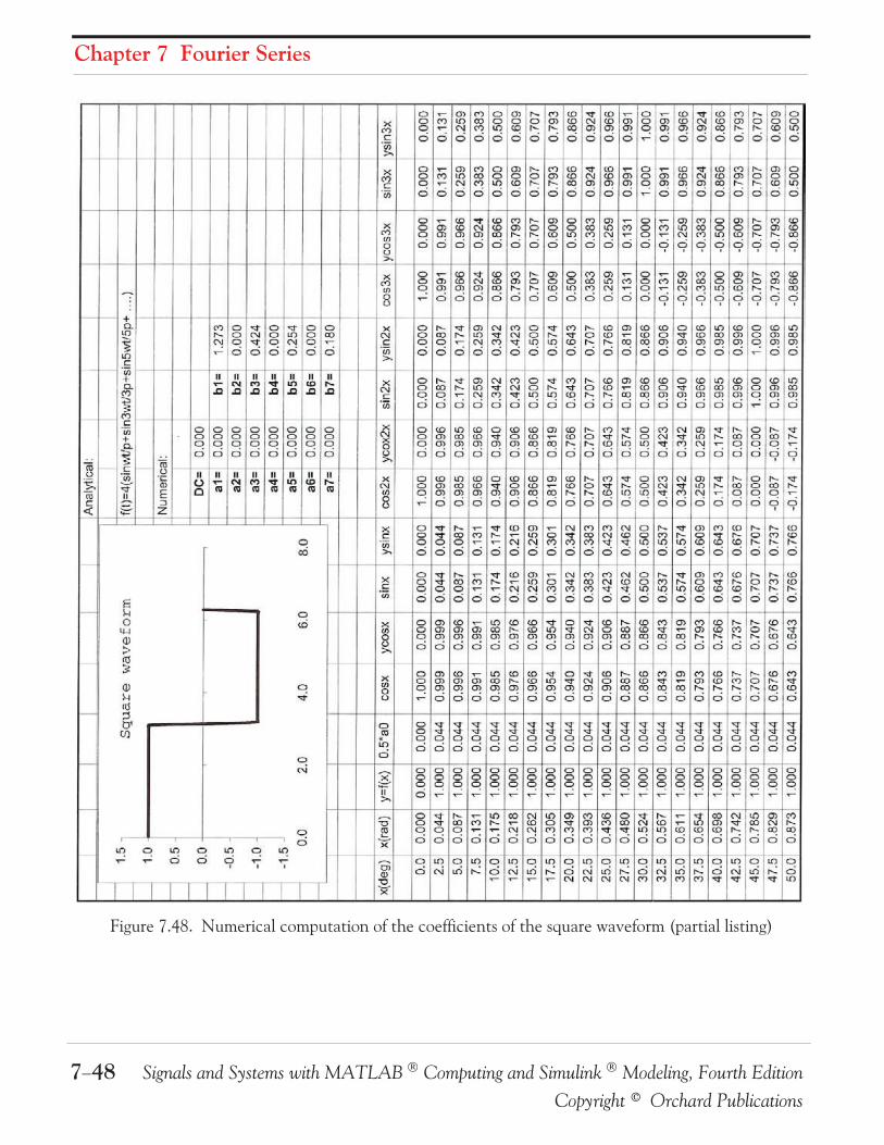
7.13 Evaluation of Fourier Coefficients Using Excel®
The use of Fourier series is not restricted to electric circuit analysis. It is also applied in the anal-ysis of the behavior of physical systems subjected to periodic disturbances. Examples includecable stress analysis in suspension bridges, and mechanical vibrations.
Quite often, it is necessary to construct the Fourier expansion of a function based on observedvalues instead of an analytic expression. Examples are meteorological or economic quantitieswhose period may be a day, a week, a month or even a year. In these situations, we need to eval-uate the integral(s) using numerical integration.
The procedure presented here, will work for both the waveforms that have an analytical solutionand those that do not. Even though we may already know the Fourier series from analyticalmethods, we can use this procedure to check our results.
Consider the waveform of shown in Figure 7.47, were we have divided it into small pulses of
width . Obviously, the more pulses we use, the better the approximation.
If the time axis is in degrees, we can choose to be and it is convenient to start at the zero
point of the waveform. Then, using a spreadsheet, such as Microsoft Excel, we can divide the
period to in intervals, and enter these values in Column of the spreadsheet.
Figure 7.47. Waveform whose analytical expression is unknown
Since the arguments of the sine and the cosine are in radians, we multiply degrees by
(3.1459...) and divide by to perform the conversion. We enter these in Column and we
denote them as . In Column we enter the corresponding values of as measured
from the waveform. In Columns and we enter the values of and the product
respectively. Similarly, we enter the values of and in Columns and respectively.
Next, we form the sums of and , we multiply these by , and we divide by to
obtain the coefficients and . To compute the coefficients of the higher order harmonics, we
° ÍÍ Í ® � Ω  � © ® � Î ¶�
� �
� ! "� # $ � �%& ' �( ) * $ �( ) *�* + , $ �* + , - .$ �( ) * $ �* + , �/ 0 1 0

Signals and Systems with MATLAB Computing and Simulink Modeling, Fourth Edition 7 47
Copyright © Orchard Publications
Evaluation of Fourier Coefficients Using MATLAB®
form the products , , , , and so on, and we enter these in subse-
quent columns of the spreadsheet.Figure 7.48 is a partial table showing the computation of the coefficients of the square waveform,and Figure 7.49 is a partial table showing the computation of the coefficients of a clipped sine
waveform. The complete tables extend to the seventh harmonic to the right and to down.
7.14 Evaluation of Fourier Coefficients Using MATLAB®
We can also use MATLAB to evaluate the coefficients of a Fourier series as illustrated with thefollowing simple example.
Example 7.8
Let where . Use the exponential Fourier series to evaluate the average value
and the first 3 harmonics using MATLAB.
Solution:
We use the following MATLAB script where the statement where represents thefunction to be integrated, is a symbolic variable for the symbolic expression, and and arenumeric values for the definite integral to b.
MATLAB displays the following:
Cn = 0 Cn = 1/2 Cn = 0 Cn = 0
The values displayed by MATLAB indicate that is the only nonzero frequency com-
ponent, and since is an even function, all coefficients in relation (7.95), Page 7 32 are
real and . Therefore,
Also, for the trigonometric Fourier series, from (7.100), Page 7 33,
$ 2 �( ) * $ 2 �* + , $ 3 �( ) * $ 3 �* + , 3 4 !� 5 5( ) *% �%# 6 # 0 # 7 # 8
# 9 � 2%5( ) * # 9# 9: # 9 � 2% %� 5 ! �2; ;; < = >: ! �2; ;; < = > !? ? ? ? ? ? < = > < = >:? 2; ; ; ; ; ; ; ; ; ; ; ; ; ; ; ; ; ; ; ; ; ; ; ; ; ; ; 5( ) *% % %/ 9 # 9 # 9:? �2; ;; �2; ;;? �% % %
Chapter 7 Fourier Series
7 48 Signals and Systems with MATLAB Computing and Simulink Modeling, Fourth Edition
Copyright © Orchard Publications
Figure 7.48. Numerical computation of the coefficients of the square waveform (partial listing)

Signals and Systems with MATLAB Computing and Simulink Modeling, Fourth Edition 7 49
Copyright © Orchard Publications
Evaluation of Fourier Coefficients Using MATLAB®
Figure 7.49. Numerical computation of the coefficients of a clipped sine waveform (partial listing)

Chapter 7 Fourier Series
7 50 Signals and Systems with MATLAB Computing and Simulink Modeling, Fourth Edition
Copyright © Orchard Publications
7.15 Summary
Any periodic waveform can be expressed as
where the first term is a constant, and represents the (average) component of .
The terms with the coefficients and together, represent the fundamental frequency
component Likewise, the terms with the coefficients and together, represent the sec-
ond harmonic component and so on. The coefficients , , and are found from the
following relations:
If a waveform has odd symmetry, that is, if it is an odd function, the series will consist of sine
terms only. We recall that odd functions are those for which
If a waveform has even symmetry, that is, if it is an even function, the series will consist of
cosine terms only, and may or may not be zero. We recall that even functions are those for
which
A periodic waveform with period , has half wave symmetry if
that is, the shape of the negative half cycle of the waveform is the same as that of the positivehalf-cycle, but inverted. If a waveform has half wave symmetry only odd (odd cosine and oddsine) harmonics will be present. In other words, all even (even cosine and even sine) harmon-ics will be zero.
The trigonometric Fourier series for the square waveform with odd symmetry is
� 5 � 5 �2; ;; / @ / A , 5( ) * 1 A , 5* + ,?9 0B?%/ 6 2 & # � 5/ C 1 C / D 1 D2 / @ / 9 1 9�2; ;; / @ �2; ; ; ; ; ; � 5 5E6 7%/ 9 �; ; ; � 5 , 5 5E( ) *6 7%1 9 �; ; ; � 5 , 5 5E* + ,6 7% � 5FF � 5%/ @� 5F � 5% G �F 5 G 2? � 5%� 5 H I; ; ; ; ; ; ; 5 �3; ;; 3 5 �J; ;; J 5* + ,? ?* + ,?* + , H I; ; ; ; ; ; ; �,; ;; , 5* + ,9 K L LB% %

Signals and Systems with MATLAB Computing and Simulink Modeling, Fourth Edition 7 51
Copyright © Orchard Publications
Summary
The trigonometric Fourier series for the square waveform with even symmetry is
The trigonometric Fourier series for the sawtooth waveform with odd symmetry is
The trigonometric Fourier series for the triangular waveform with odd symmetry is
The trigonometric Fourier series for the half wave rectifier with no symmetry is
The trigonometric form of the Fourier series for the full wave rectifier with even symmetry is
The Fourier series are often expressed in exponential form as
where the coefficients are related to the trigonometric form coefficients as
The coefficients, except , are complex, and appear as complex conjugate pairs, that is,
In general, for ,
� 5 H I; ; ; ; ; ; ; ( ) * 5 �3; ; ;F 3 5 �J; ;; J 5( ) * F?( ) * H I; ; ; ; ; ; ; �F 9 0:7M M M M M M M M M M M M M M M M �,; ;; ,( ) * 59 K L LB% %� 5 2 I; ; ; ; ; ; ; 5 �2; ;; 2 5 �3; ;; 3 5* + , �H; ;; H 5 ?* + ,F?* + ,F* + , 2 I; ; ; ; ; ; ; �F 9 0: �,; ;; , 5* + ,% %
� 5 I 7; ; ; ; ; ; ; * + , 5 �N; ;;F 3 5 �2 J; ; ; ; ; ; J 5* + , �H N; ; ; ; ;; O 5* + , ?F?* + , I 7; ; ; ; ; ; ; �F 9 0:7M M M M M M M M M M M M M M M M �, 7; ; ; ; ; ,* + , 59 K L LB% %� 5 I; ; ; ; I 2; ; ; ; 5* + , I; ; ; ; 2 5( ) *3; ; ; ; ; ; ; ; ; ; ; ; ; H 5( ) *� J; ; ; ; ; ; ; ; ; ; ; ; ; 4 5( ) *3 J; ; ; ; ; ; ; ; ; ; ; ; ; 5( ) *4 3; ; ; ; ; ; ; ; ; ; ; ; ;? ? ? ?F?%
� 5 2 I; ; ; ; ; ; ; H I; ; ; ; ; ; ; �, D �F; ; ; ; ; ; ; ; ; ; ; ; ; ; ; ; ; ; ; , 5( ) *9 7 P QBF%� 5 # DR < = 7 >: # CR < = >: # @ # C < = > # D < = 7 >? ? ? ? ? ?%# S # 9: �2; ;; / 9 1 9T; ; ; ; ;F �2; ;; / 9 T 1 9?% %# 9 �2; ;; / 9 1 9T; ; ; ; ;? �2; ;; / 9 TF 1 9% %# @ �2; ;; / @%# S # @ # 9: # 9%�

Chapter 7 Fourier Series
7 52 Signals and Systems with MATLAB Computing and Simulink Modeling, Fourth Edition
Copyright © Orchard Publications
We can derive the trigonometric Fourier series from the exponential series from the relations
and
For even functions, all coefficients are real
For odd functions, all coefficients are imaginary
If there is half wave symmetry, for
always
A line spectrum is a plot that shows the amplitudes of the harmonics on a frequency scale.
The frequency components of a recurrent rectangular pulse follow a form.
he line spectrum of an impulse train consists of a train of equal amplitude, and are equallyspaced harmonics.
he value of a waveform consisting of sinusoids of different frequencies, is equal to the
square root of the sum of the squares of the values of each sinusoid. Thus,
or
We can compute the average power of a Fourier series from the relation
We can evaluate the Fourier coefficients of a function based on observed values instead of ananalytic expression using numerical evaluations with the aid of a spreadsheet.
# 9 �G; ; ; � 5 < = 9 >: 5E6 U �2; ; ; ; ; ; � 5 < = 9 >: 5E6 7% %/ 9 # 9 # 9:?%1 9 T # 9 # 9:F%# S# S# 9 !% , < V < ,%# 9: # 9% �* + , �W X Y W X YZ [ \ ] Z @ D Z C [ \ ]D Z D [ \ ]D Z ^ [ \ ]D? ? ? ?%Z [ \ ] Z @ D �2; ;; Z C _D �2; ;; Z D _D �2; ;; Z ^ _D? ? ? ?%` a b c ` L d ` 0 a b c ` 7 a b c? ? ?% e L d Z L d e C [ \ ] Z C [ \ ] C( ) * e D [ \ ] Z D [ \ ] D( ) *? ? ?%

Signals and Systems with MATLAB Computing and Simulink Modeling, Fourth Edition 7 53
Copyright © Orchard Publications
Exercises
7.16 Exercises
1. Compute the first 5 components of the trigonometric Fourier series for the waveform shown
below. Assume .
2. Compute the first 5 components of the trigonometric Fourier series for the waveform shown
below. Assume .
3. Compute the first 5 components of the exponential Fourier series for the waveform shown
below. Assume .
4.Compute the first 5 components of the exponential Fourier series for the waveform shown
below. Assume .
�%f g
hi g�%
j klm nop
qr m nop
q m nr s rt s

Chapter 7 Fourier Series
7 54 Signals and Systems with MATLAB Computing and Simulink Modeling, Fourth Edition
Copyright © Orchard Publications
5. Compute the first 5 components of the exponential Fourier series for the waveform shown
below. Assume .
6. Compute the first 5 components of the exponential Fourier series for the waveform shown
below. Assume .
opqrm n
opq kr
rm n

Signals and Systems with MATLAB Computing and Simulink Modeling, Fourth Edition 7 55
Copyright © Orchard Publications
Solutions to End of Chapter Exercises
7.17 Solutions to End of Chapter Exercises
1.
This is an even function; therefore, the series consists of cosine terms only. There is no half
wave symmetry and the average ( component) is not zero. We will integrate from to
and multiply by . Then,
(1)
From tables of integrals,
and thus (1) becomes
and since for all integer ,
(2)
We cannot evaluate the average from (2); we must use (1). Then, for ,
or
We observe from (2) that for , . Then,
u krv k r w w w w k
st t sx y qz { | z} } } ~} } } } n � n� � � n�� z ~ �} } } } } } } n � n� � � n��p p� { �� � � �� o{ �} } } } } { �� � � � {} }} {� � � ��p{ | z ~ �} } } } } } } o� �} } } } } � n� � � n�} }} � n� � �� � z ~ �} } } } } } } o� �} } } } } �� � � n�} }} � n o� �} } } } }� q�� � ��p p� n� � � qp �{ | z ~ �} } } } } } } o� �} } } } } �� � � o� �} } } } }� z ~� � �} } } } } } } } } } } � o�� � �p po z { � � qpoz} }} { � z ~z �} } } } } } } } } n n�� ~ �} } } } } n �z} } } } � ~ �} } } } } �z} } } } }p p po z { � ~ zp� � � � �p { | � � � |� qpm � � � o { � � ~ �} } } } } } }� m � � �p � { � � ~�� � �} } } } } } } } } } } m � � � � { � � ~� � �} } } } } } } } } } }� m � � �p � { � � ~�� � �} } } } } } } } } } }pp ppp p

Chapter 7 Fourier Series
7 56 Signals and Systems with MATLAB Computing and Simulink Modeling, Fourth Edition
Copyright © Orchard Publications
and so on. Therefore,
2.
This is an even function; therefore, the series consists of cosine terms only. There is no half
wave symmetry and the average ( component) is not zero.
(1)
and with
relation (1) above simplifies to
and since for all integer ,
We observe that the fourth harmonic and all its multiples are zero. Therefore,
m n oz} }} { � � ~ �} } } } } } } n� � � o�} }} � n� � � oz �} } } } }} � n� � � o� �} } } } }} � n� � �� � � �� ~ z} } } } � ~} } } } } } } o� �} } } } } � n� � �| � � ���p pu krv k s rw w w w w w w k s � sx y~ � � � { � � oz} }} { � ~ � � {� � � � � �} } } } } } } } } } } } } } } } } z ~ z z ~�z} } } } } } } } } } } } } } } } } } } } } } } } } } } } } } } } } } } } } } } } } } } } } } } } } } } } } } } } } } } } } } } } � ~ zz} } } } } } } } } } } } } } } } } } } } } } } } } } } � ~�} } } } } } }p p p p p{ | z} } } z ~} } } } } } } n � n� � � n�� � z} } } ~ � n� � � n���p� { �� � � �� o{ �} } } } } { �� � � � {} }} {� � � �� o{ �} } } } } { � { � { �� � ��� � �p p
{ | � ~ �} } } } } } } o� �} } } } } � n� � � � n � n� � �� � � z ~�} } } } } } } � n �� � ��p � ~� � �} } } } } } } } } } } � z} } } } } }� � � � z} } } } } } � z} } } } } }� � � o q��� z ~�} } } } } } } �� � � � z} } } } } }� � ���p� n� � � qp �{ | � ~� � �} } } } } } } } } } } � z} } } } } }� � � z ~�} } } } } } } � z} } } } } }� � � � ~� � �} } } } } } } } } } }� z ~�} } } } } } } � z} } } } } }� � ��� � ~� � �} } } } } } } } } } } � z} } } } } }� � � o�p pm � � � o { � � ~ �} } } } } } } q o� � ~ �} } } } } } }� m � � �p p z { � � ~� �} } } } } } } } } o� o� z ~ �} } } } } } }�p pp pm � � � � { � � ~� �} } } } } } } } } q o� � ~� �} } } } } } } } }�p m � � �p � { � � ~�� � �} } } } } } } } } } } o o�p qp p p

Signals and Systems with MATLAB Computing and Simulink Modeling, Fourth Edition 7 57
Copyright © Orchard Publications
Solutions to End of Chapter Exercises
3.
This is neither an even nor an odd function and has no half wave symmetry; therefore, the
series consists of both cosine and sine terms. The average ( component) is not zero. Then,
and with
The value is
For ,
Recalling that
for , and for , . Then,
and
By substitution into
we find that
m n � ~�} } } } } } } � ~ �} } } } } } } n� � � oz} }} z n� � � o�} }} � n� � �� � ��pqr m n
z x yy | oz} } } } } } m n � � | � n�� �popy | oz} } } } } } m n � � | � n�� � oz} } } } } } ~ � � | � n�� q � � | � n��� ~z} } } } } } � � | � n��p ppx y y � ~z} } } } } } � � n�� ~z} } } } } } n � ~ z} } } }p p p� q y | ~z} } } } } } � � | � n�� ~¡ z� �} } } } } } } } } } } } } } } � � | � �p ~¡ z �} } } } } } } } } } } } o � � | �p p� � | � ¡ �� � ��� � �p� � � � �p � � | op � � � �p � � | o�py | � � � |� ~¡ z �} } } } } } } } } } } } o o� qp py | � � �� ~¡ z �} } } } } } } } } } } } o o�� ~¡ �} } } } } } } }p pm n y ¢£ � � � � y ¤£ � � � y ¥ y ¤ � � � y ¢ � � � �� � � � � �p

Chapter 7 Fourier Series
7 58 Signals and Systems with MATLAB Computing and Simulink Modeling, Fourth Edition
Copyright © Orchard Publications
The minus ( sign of the first two terms within the parentheses results from the fact that
. For instance, since , it follows that . We
observe that is complex, as expected, since there is no symmetry.
4.
This is the same waveform as in Exercise 3 where the component has been removed.
Then,
It is also the same waveform as in Example 7.3, Page 7 34, except that the amplitude is
halved. This waveform is an odd function and thus the expression for is imaginary.
5.
This is the same waveform as in Exercise 3 where the vertical axis has been shifted to make
the waveform an even function. Therefore, for this waveform is real. Then,
The value is
For ,
m n ~ z} } } } ~¡ } } } } } o�} }} � � � � � � � �� � � � o�} }} � � � �� � ��py | y |p y � z ~ ¡p y � y � z ~� ¡p pm nq m nr s rt s x ym n ~¡ } } } } } o�} }} � � � � � � � �� � � � o�} }} � � � �� � �p m n
q rm nz� z� y |y | oz} } } } } } m n � � | � n� ~z} } } } } } � � | � n� ��ppx y y � ~z} } } } } } n �� ~z} } } } } } z} } } z} } }� ~ z} } } }p p p� q
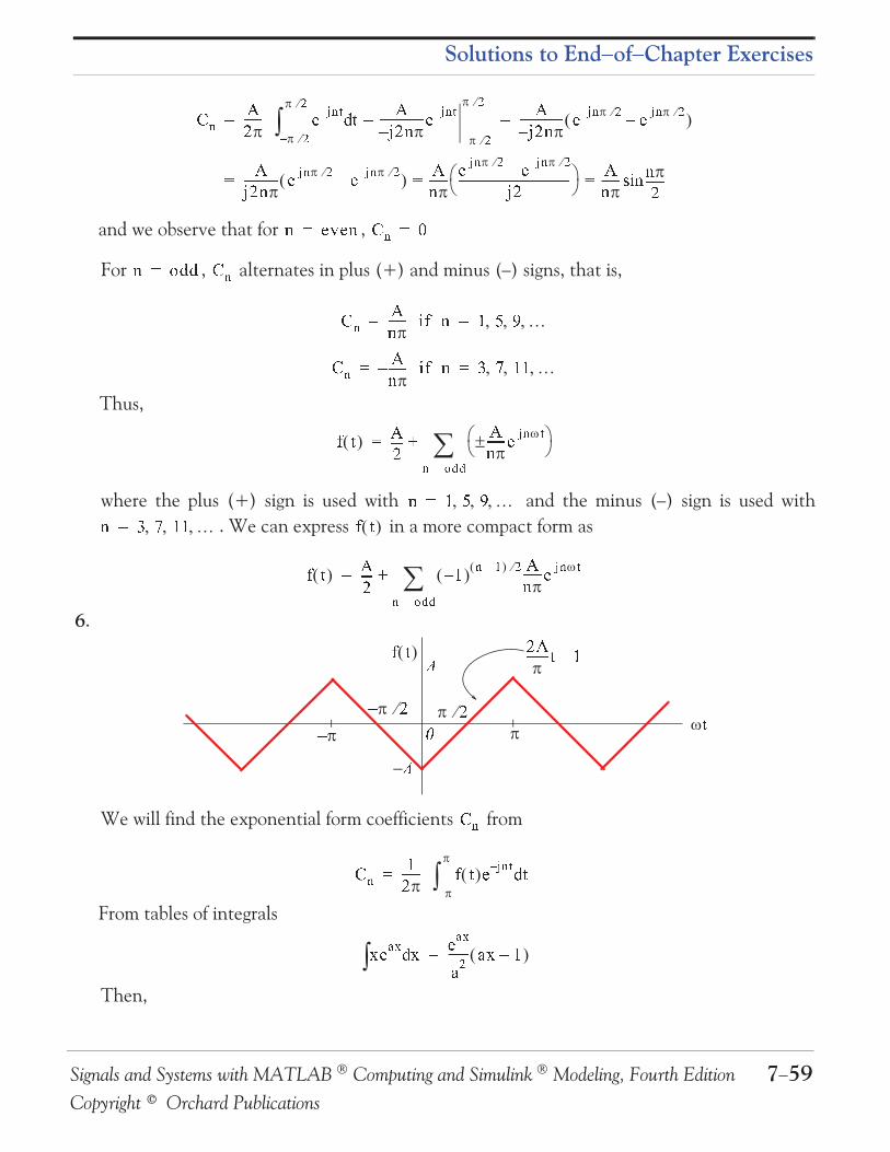
Signals and Systems with MATLAB Computing and Simulink Modeling, Fourth Edition 7 59
Copyright © Orchard Publications
Solutions to End of Chapter Exercises
and we observe that for ,
For , alternates in plus (+) and minus ( ) signs, that is,
Thus,
where the plus (+) sign is used with and the minus ( ) sign is used with
. We can express in a more compact form as
6.
We will find the exponential form coefficients from
From tables of integrals
Then,
y | ~z} } } } } } � � | � n� �� ~¡ z� �} } } } } } } } } } } } } } } � � | � ��p ~¡ z� �} } } } } } } } } } } } } } } � � | � � � | ��p p~¡ z �} } } } } } } } } } } } � � | � � � | � � ~�} } } } } } � � | � � � | � �¡ z} } } } } } } } } } } } } } } } } } } } } } } } } } } } } } } } } } } } } } ~�} } } } } } � z} } } } } }� � �p pp � � � � �p y | qp� � � �p y | y | ~�} } } } } } � m � o � �p py | ~�} } } } } }� � m � � � o op pm n ~ z} } } } ~�} } } } } } � � | �| � � ���p � o � �p� � � o op m nm n ~ z} } } } o� | � � ~�} } } } } } � � | �| � � ���p¦ kl
lm n z ~} } } } } } } n o�� � z z
y |y | oz} } } } } } m n � � | � n� p� � § ¨ �� � § ¨{ �} } } } } } } { � o�p

Chapter 7 Fourier Series
7 60 Signals and Systems with MATLAB Computing and Simulink Modeling, Fourth Edition
Copyright © Orchard Publications
Integrating and rearranging terms we obtain
and since for all integer ,
For , and for , , and
Also, by inspection, the component . Then,
The coefficients of the terms and are positive because all coefficients of are
real. This is to be expected since is an even function. It also has half wave symmetry and
thus for as we’ve found.
y | oz} } } } } } z ~} } } } } } }� n o� � � | � n� � z ~} } } } } } } n o� � � | � n���py | oz} } } } } } � ~� �} } } } } } } } }� � ~� �} } } } } } } } } � � � | � � | �¡ z} } } } } } } } } } } } } } } } } } } } } } } } } } } } � � | � � | � z} } } } } } } } } } } } } } } } } } } } } } } } } } } }� z ~�} } } } } } } � � | � � | �¡ z} } } } } } } } } } } } } } } } } } } } } } } } } } } }��p � ~z � � �} } } } } } } } } } } } } } o� � �� � � �� � � � z} } } } } } �� � ��� �p �� � � qp �y | z ~� � �} } } } } } } } } } } �� � � o�p� � � � �p y | qp � � � �p �� � � o�p y | �� ~� � �} } } } } } } } } } }px y y � qpm n � ~ �} } } } } } }� o�} }} � � � � � � � � � � o�} }} � � � �� � � � �p � � � � � � � y |m ny | qp � � � � �p