arbitrage-free svi volatility surfaces · introduction static arbitrage svi formulations ssvi...

Introduction Static arbitrage SVI formulations SSVI Numerics

Arbitrage-free SVI volatility surfaces

Jim Gatheral

Center for the Study of Finance and InsuranceOsaka University, December 26, 2012

(Including joint work with Antoine Jacquier)


Outline

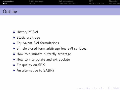
History of SVI

Static arbitrage

Equivalent SVI formulations

Simple closed-form arbitrage-free SVI surfaces

How to eliminate butterfly arbitrage

How to interpolate and extrapolate

Fit quality on SPX

An alternative to SABR?


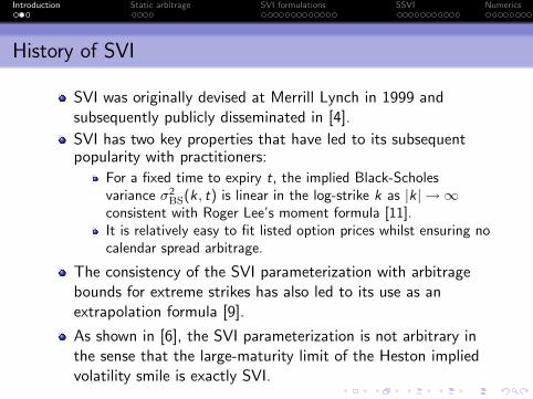
History of SVI

SVI was originally devised at Merrill Lynch in 1999 andsubsequently publicly disseminated in [4].

SVI has two key properties that have led to its subsequentpopularity with practitioners:

For a fixed time to expiry t, the implied Black-Scholesvariance σ2

BS(k , t) is linear in the log-strike k as |k| → ∞consistent with Roger Lee’s moment formula [11].It is relatively easy to fit listed option prices whilst ensuring nocalendar spread arbitrage.

The consistency of the SVI parameterization with arbitragebounds for extreme strikes has also led to its use as anextrapolation formula [9].

As shown in [6], the SVI parameterization is not arbitrary inthe sense that the large-maturity limit of the Heston impliedvolatility smile is exactly SVI.


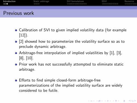
Previous work

Calibration of SVI to given implied volatility data (for example[12]).

[2] showed how to parameterize the volatility surface so as topreclude dynamic arbitrage.

Arbitrage-free interpolation of implied volatilities by [1], [3],[8], [10].

Prior work has not successfully attempted to eliminate staticarbitrage.

Efforts to find simple closed-form arbitrage-freeparameterizations of the implied volatility surface are widelyconsidered to be futile.


Notation

Given a stock price process (St)t≥0 with natural filtration(Ft)t≥0, the forward price process (Ft)t≥0 is Ft := E (St |F0).

For any k ∈ R and t > 0, CBS(k , σ2t) denotes theBlack-Scholes price of a European Call option on S with strikeFtek , maturity t and volatility σ > 0.

σBS(k, t) denotes Black-Scholes implied volatility.

Total implied variance is w(k, t) = σ2BS(k , t)t.

The implied variance v(k, t) = σ2BS(k , t) = w(k, t)/t.

The map (k , t) 7→ w(k , t) is the volatility surface.

For any fixed expiry t > 0, the function k 7→ w(k , t)represents a slice.


Characterisation of static arbitrage

Definition 2.1

A volatility surface is free of static arbitrage if and only if thefollowing conditions are satisfied:

(i) it is free of calendar spread arbitrage;

(ii) each time slice is free of butterfly arbitrage.


Calendar spread arbitrage

Lemma 2.2

If dividends are proportional to the stock price, the volatilitysurface w is free of calendar spread arbitrage if and only if

∂tw(k , t) ≥ 0, for all k ∈ R and t > 0.

Thus there is no calendar spread arbitrage if there are nocrossed lines on a total variance plot.


Butterfly arbitrage

Definition 2.3

A slice is said to be free of butterfly arbitrage if the correspondingdensity is non-negative.

Now introduce the function g : R→ R defined by

g(k) :=

(1− kw ′(k)

2w(k)

)2

− w ′(k)2

4

(1

w(k)+

1

4

)+

w ′′(k)

2.

Lemma 2.4

A slice is free of butterfly arbitrage if and only if g(k) ≥ 0 for allk ∈ R and lim

k→+∞d+(k) = −∞.


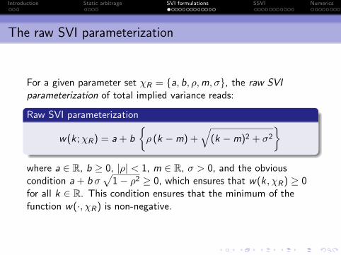
The raw SVI parameterization

For a given parameter set χR = {a, b, ρ,m, σ}, the raw SVIparameterization of total implied variance reads:

Raw SVI parameterization

w(k ;χR) = a + b

{ρ (k −m) +

√(k −m)2 + σ2

}where a ∈ R, b ≥ 0, |ρ| < 1, m ∈ R, σ > 0, and the obviouscondition a + b σ

√1− ρ2 ≥ 0, which ensures that w(k , χR) ≥ 0

for all k ∈ R. This condition ensures that the minimum of thefunction w(·, χR) is non-negative.


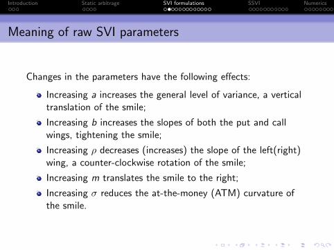
Meaning of raw SVI parameters

Changes in the parameters have the following effects:

Increasing a increases the general level of variance, a verticaltranslation of the smile;

Increasing b increases the slopes of both the put and callwings, tightening the smile;

Increasing ρ decreases (increases) the slope of the left(right)wing, a counter-clockwise rotation of the smile;

Increasing m translates the smile to the right;

Increasing σ reduces the at-the-money (ATM) curvature ofthe smile.


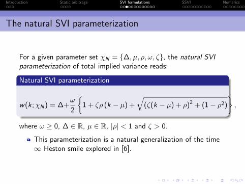
The natural SVI parameterization

For a given parameter set χN = {∆, µ, ρ, ω, ζ}, the natural SVIparameterization of total implied variance reads:

Natural SVI parameterization

w(k ;χN) = ∆+ω

2

{1 + ζρ (k − µ) +

√(ζ(k − µ) + ρ)2 + (1− ρ2)

},

where ω ≥ 0, ∆ ∈ R, µ ∈ R, |ρ| < 1 and ζ > 0.

This parameterization is a natural generalization of the time∞ Heston smile explored in [6].


The SVI Jump-Wings (SVI-JW) parameterization

Neither the raw SVI nor the natural SVI parameterizations areintuitive to traders.

There is no reason to expect these parameters to beparticularly stable.

The SVI-Jump-Wings (SVI-JW) parameterization of theimplied variance v (rather than the implied total variance w)was inspired by a similar parameterization attributed to TimKlassen, then at Goldman Sachs.


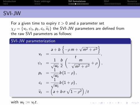
SVI-JW

For a given time to expiry t > 0 and a parameter setχJ = {vt , ψt , pt , ct , vt} the SVI-JW parameters are defined fromthe raw SVI parameters as follows:

SVI-JW parameterization

vt =a + b

{−ρm +

√m2 + σ2

}t

,

ψt =1√

wt

b

2

(− m√

m2 + σ2+ ρ

),

pt =1√

wtb (1− ρ) ,

ct =1√

wtb (1 + ρ) ,

vt =(

a + b σ√

1− ρ2)/t

with wt := vtt.


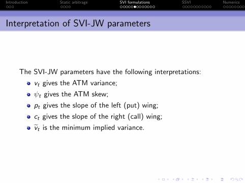
Interpretation of SVI-JW parameters

The SVI-JW parameters have the following interpretations:

vt gives the ATM variance;

ψt gives the ATM skew;

pt gives the slope of the left (put) wing;

ct gives the slope of the right (call) wing;

vt is the minimum implied variance.


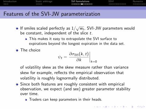
Features of the SVI-JW parameterization

If smiles scaled perfectly as 1/√

wt , SVI-JW parameters wouldbe constant, independent of the slice t.

This makes it easy to extrapolate the SVI surface toexpirations beyond the longest expiration in the data set.

The choice

ψt =∂σBS(k, t)

∂k

∣∣∣∣k=0

of volatility skew as the skew measure rather than varianceskew for example, reflects the empirical observation thatvolatility is roughly lognormally distributed.

Since both features are roughly consistent with empiricalobservation, we expect (and see) greater parameter stabilityover time.

Traders can keep parameters in their heads.


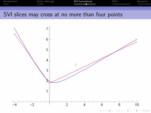
SVI slices may cross at no more than four points

�

-4 -2 2 4 6 8 10

1

2

3

4

5

6

7


Condition for no calendar spread arbitrage

Lemma 3.1

Two raw SVI slices admit no calendar spread arbitrage if a certainquartic polynomial has no real root.


Ferrari Cardano

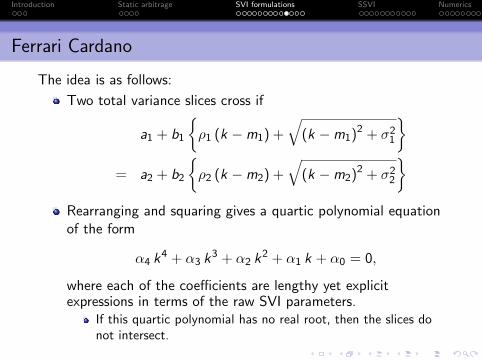
The idea is as follows:

Two total variance slices cross if

a1 + b1

{ρ1 (k −m1) +

√(k −m1)2 + σ2

1

}= a2 + b2

{ρ2 (k −m2) +

√(k −m2)2 + σ2

2

}Rearranging and squaring gives a quartic polynomial equationof the form

α4 k4 + α3 k3 + α2 k2 + α1 k + α0 = 0,

where each of the coefficients are lengthy yet explicitexpressions in terms of the raw SVI parameters.

If this quartic polynomial has no real root, then the slices donot intersect.


SVI butterfly arbitrage

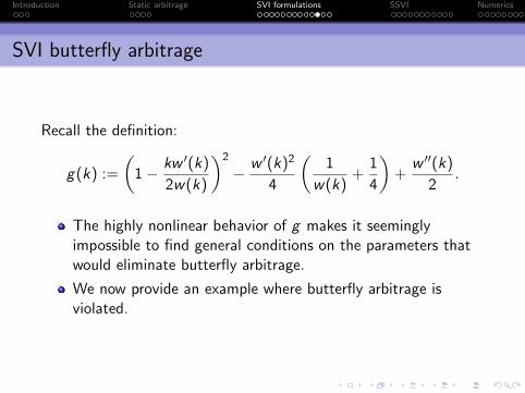
Recall the definition:

g(k) :=

(1− kw ′(k)

2w(k)

)2

− w ′(k)2

4

(1

w(k)+

1

4

)+

w ′′(k)

2.

The highly nonlinear behavior of g makes it seeminglyimpossible to find general conditions on the parameters thatwould eliminate butterfly arbitrage.

We now provide an example where butterfly arbitrage isviolated.


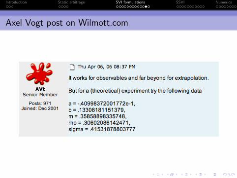
Axel Vogt post on Wilmott.com


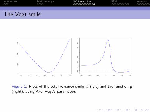
The Vogt smile

−1.5 −1.0 −0.5 0.0 0.5 1.0 1.5

0.05

0.10

0.15

−1.5 −1.0 −0.5 0.0 0.5 1.0 1.5

0.0

0.2

0.4

0.6

0.8

1.0

1.2

1.4

Figure 1: Plots of the total variance smile w (left) and the function g(right), using Axel Vogt’s parameters


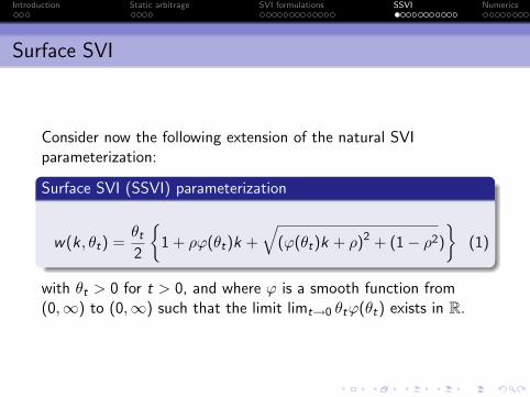
Surface SVI

Consider now the following extension of the natural SVIparameterization:

Surface SVI (SSVI) parameterization

w(k , θt) =θt2

{1 + ρϕ(θt)k +

√(ϕ(θt)k + ρ)2 + (1− ρ2)

}(1)

with θt > 0 for t > 0, and where ϕ is a smooth function from(0,∞) to (0,∞) such that the limit limt→0 θtϕ(θt) exists in R.


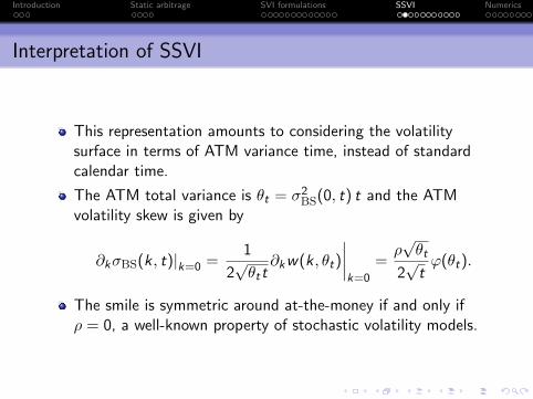
Interpretation of SSVI

This representation amounts to considering the volatilitysurface in terms of ATM variance time, instead of standardcalendar time.

The ATM total variance is θt = σ2BS(0, t) t and the ATM

volatility skew is given by

∂kσBS(k , t)|k=0 =1

2√θtt

∂kw(k , θt)

∣∣∣∣k=0

=ρ√θt

2√

tϕ(θt).

The smile is symmetric around at-the-money if and only ifρ = 0, a well-known property of stochastic volatility models.


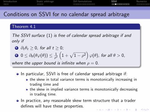
Conditions on SSVI for no calendar spread arbitrage

Theorem 4.1

The SSVI surface (1) is free of calendar spread arbitrage if andonly if

1 ∂tθt ≥ 0, for all t ≥ 0;

2 0 ≤ ∂θ(θϕ(θ)) ≤ 1ρ2

(1 +

√1− ρ2

)ϕ(θ), for all θ > 0,

where the upper bound is infinite when ρ = 0.

In particular, SSVI is free of calendar spread arbitrage if:the skew in total variance terms is monotonically increasing intrading time andthe skew in implied variance terms is monotonically decreasingin trading time.

In practice, any reasonable skew term structure that a traderdefines will have these properties.


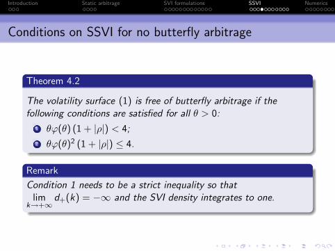
Conditions on SSVI for no butterfly arbitrage

Theorem 4.2

The volatility surface (1) is free of butterfly arbitrage if thefollowing conditions are satisfied for all θ > 0:

1 θϕ(θ) (1 + |ρ|) < 4;

2 θϕ(θ)2 (1 + |ρ|) ≤ 4.

Remark

Condition 1 needs to be a strict inequality so thatlim

k→+∞d+(k) = −∞ and the SVI density integrates to one.


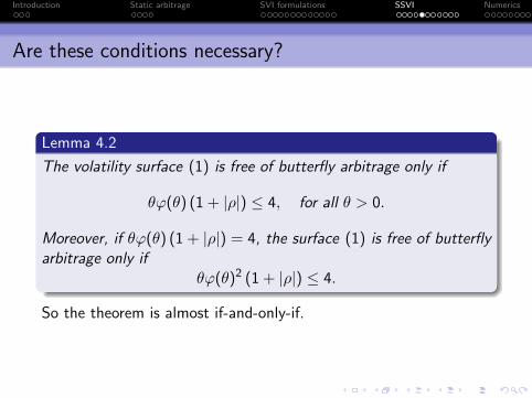
Are these conditions necessary?

Lemma 4.2

The volatility surface (1) is free of butterfly arbitrage only if

θϕ(θ) (1 + |ρ|) ≤ 4, for all θ > 0.

Moreover, if θϕ(θ) (1 + |ρ|) = 4, the surface (1) is free of butterflyarbitrage only if

θϕ(θ)2 (1 + |ρ|) ≤ 4.

So the theorem is almost if-and-only-if.


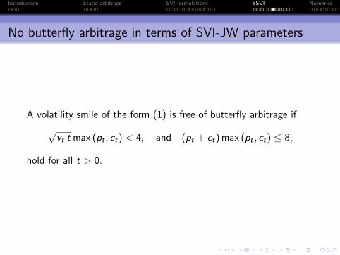
No butterfly arbitrage in terms of SVI-JW parameters

A volatility smile of the form (1) is free of butterfly arbitrage if

√vt t max (pt , ct) < 4, and (pt + ct) max (pt , ct) ≤ 8,

hold for all t > 0.


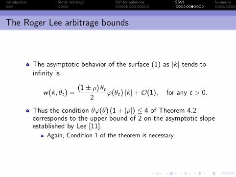
The Roger Lee arbitrage bounds

The asymptotic behavior of the surface (1) as |k | tends toinfinity is

w(k , θt) =(1± ρ) θt

2ϕ(θt) |k |+O(1), for any t > 0.

Thus the condition θϕ(θ) (1 + |ρ|) ≤ 4 of Theorem 4.2corresponds to the upper bound of 2 on the asymptotic slopeestablished by Lee [11].

Again, Condition 1 of the theorem is necessary.


No static arbitrage with SSVI

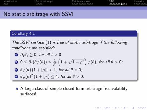
Corollary 4.1

The SSVI surface (1) is free of static arbitrage if the followingconditions are satisfied:

1 ∂tθt ≥ 0, for all t > 0

2 0 ≤ ∂θ(θϕ(θ)) ≤ 1ρ2

(1 +

√1− ρ2

)ϕ(θ), for all θ > 0;

3 θϕ(θ) (1 + |ρ|) < 4, for all θ > 0;

4 θϕ(θ)2 (1 + |ρ|) ≤ 4, for all θ > 0.

A large class of simple closed-form arbitrage-free volatilitysurfaces!


A Heston-like surface

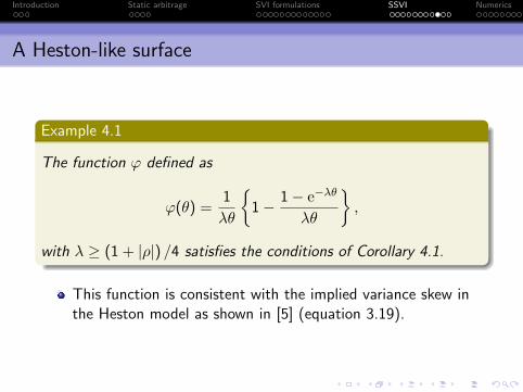
Example 4.1

The function ϕ defined as

ϕ(θ) =1

λθ

{1− 1− e−λθ

λθ

},

with λ ≥ (1 + |ρ|) /4 satisfies the conditions of Corollary 4.1.

This function is consistent with the implied variance skew inthe Heston model as shown in [5] (equation 3.19).


A power-law surface

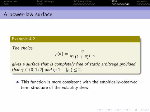
Example 4.2

The choiceϕ(θ) =

η

θγ (1 + θ)1−γ

gives a surface that is completely free of static arbitrage providedthat γ ∈ (0, 1/2] and η (1 + |ρ|) ≤ 2.

This function is more consistent with the empirically-observedterm structure of the volatility skew.


Even more flexibility...

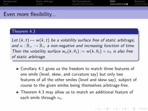
Theorem 4.3

Let (k , t) 7→ w(k , t) be a volatility surface free of static arbitrage,and α : R+ → R+ a non-negative and increasing function of time.Then the volatility surface wα(k , θt) := w(k , θt) + αt is also freeof static arbitrage.

Corollary 4.1 gives us the freedom to match three features ofone smile (level, skew, and curvature say) but only twofeatures of all the other smiles (level and skew say), subject ofcourse to the given smiles being themselves arbitrage-free.

Theorem 4.3 may allow us to match an additional feature ofeach smile through αt .


How to eliminate butterfly arbitrage

We have shown how to define a volatility smile (SSVI) that isfree of butterfly arbitrage.

This smile is completely defined given three observables.

The ATM volatility and ATM skew are obvious choices for twoof them.The most obvious choice for the third observable in equitymarkets would be the asymptotic slope for k negative and inFX markets and interest rate markets, perhaps the ATMcurvature of the smile might be more appropriate.


How to fix butterfly arbitrage

Supposing we choose to fix the SVI-JW parameters vt , ψt

and pt of a given SVI smile, we may guarantee a smile withno butterfly arbitrage by choosing the remainingparameters c ′t and v ′t according to SSVI as

c ′t = pt + 2ψt , and v ′t = vt4ptc ′t

(pt + c ′t)2.

That is, given a smile defined in terms of its SVI-JWparameters, we are guaranteed to be able to eliminatebutterfly arbitrage by changing the call wing ct and theminimum variance vt , both parameters that are hard tocalibrate with available quotes in equity options markets.


Example: Fixing the Vogt smile

The SVI-JW parameters corresponding to the Vogt smile are:

(vt , ψt , pt , ct , vt)

= (0.01742625,−0.1752111, 0.6997381, 1.316798, 0.0116249) .

We know then that choosing(ct , vt) = (0.3493158, 0.01548182) must give a smile free ofbutterfly arbitrage.

There must exist some pair of parameters {ct , vt} withct ∈ (0.349, 1.317) and vt ∈ (0.0116, 0.0155) such that thenew smile is free of butterfly arbitrage and is as close aspossible to the original one in some sense.


Numerical optimization

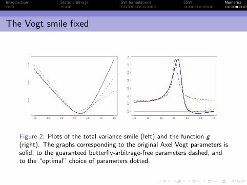
In this particular case, choosing the objective function as thesum of squared option price differences plus a large penalty forbutterfly arbitrage, we arrive at the following “optimal”choices of the call wing and minimum variance parametersthat still ensure no butterfly arbitrage:

(ct , vt) = (0.8564763, 0.0116249) .

Note that the optimizer has left vt unchanged but hasdecreased the call wing.

The resulting smiles and plots of the function g are shown inFigure 2.


The Vogt smile fixed

−1.5 −1.0 −0.5 0.0 0.5 1.0 1.5

0.05

0.10

0.15

−1.5 −1.0 −0.5 0.0 0.5 1.0 1.5

0.0

0.2

0.4

0.6

0.8

1.0

1.2

1.4

Figure 2: Plots of the total variance smile (left) and the function g(right). The graphs corresponding to the original Axel Vogt parameters issolid, to the guaranteed butterfly-arbitrage-free parameters dashed, andto the “optimal” choice of parameters dotted.


Why extra flexibility may not help

The additional flexibility potentially afforded to us through theparameter αt of Theorem 4.3 sadly does not help us with theVogt smile.

For αt to help, we must have αt > 0; it is straightforward toverify that this translates to the condition vt (1− ρ2) < vt

which is violated in the Vogt case.


Quantifying lines crossing

Consider two SVI slices with parameters χ1 and χ2 wheret2 > t1.

We first compute the points ki (i = 1, . . . , n) with n ≤ 4 atwhich the slices cross, sorting them in increasing order. Ifn > 0, we define the points ki as

k1 := k1 − 1,

ki :=1

2(ki−1 + ki ), if 2 ≤ i ≤ n,

kn+1 := kn + 1.

For each of the n + 1 points ki , we compute the amounts ci

by which the slices cross:

ci = max[0,w(ki , χ1)− w(ki , χ2)

].


Crossedness

Definition 5.1

The crossedness of two SVI slices is defined as the maximum ofthe ci (i = 1, . . . , n). If n = 0, the crossedness is null.


A sample calibration recipe

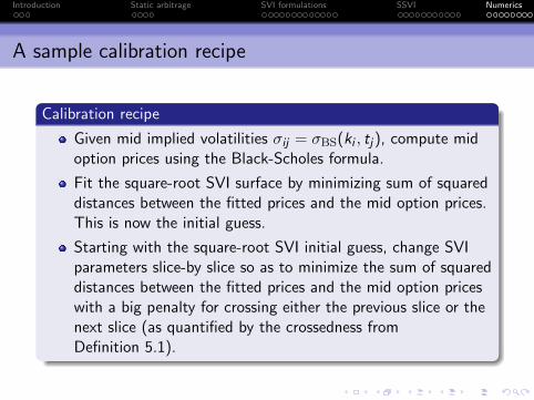
Calibration recipe

Given mid implied volatilities σij = σBS(ki , tj), compute midoption prices using the Black-Scholes formula.

Fit the square-root SVI surface by minimizing sum of squareddistances between the fitted prices and the mid option prices.This is now the initial guess.

Starting with the square-root SVI initial guess, change SVIparameters slice-by slice so as to minimize the sum of squareddistances between the fitted prices and the mid option priceswith a big penalty for crossing either the previous slice or thenext slice (as quantified by the crossedness fromDefinition 5.1).


Interpolation

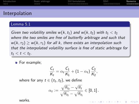
Lemma 5.1

Given two volatility smiles w(k, t1) and w(k , t2) with t1 < t2

where the two smiles are free of butterfly arbitrage and such thatw(k , τ2) ≥ w(k, τ1) for all k, there exists an interpolation suchthat the interpolated volatility surface is free of static arbitrage fort1 < t < t2.

For example;

Ct

Kt= αt

C1

K1+ (1− αt)

C2

K2,

where for any t ∈ (t1, t2), we define

αt :=

√θt2 −

√θt√

θt2 −√θt1

∈ [0, 1] .

works.


A possible choice of extrapolation

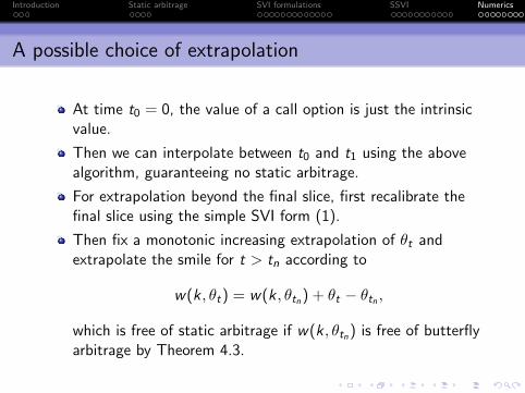
At time t0 = 0, the value of a call option is just the intrinsicvalue.

Then we can interpolate between t0 and t1 using the abovealgorithm, guaranteeing no static arbitrage.

For extrapolation beyond the final slice, first recalibrate thefinal slice using the simple SVI form (1).

Then fix a monotonic increasing extrapolation of θt andextrapolate the smile for t > tn according to

w(k , θt) = w(k , θtn) + θt − θtn ,

which is free of static arbitrage if w(k, θtn) is free of butterflyarbitrage by Theorem 4.3.


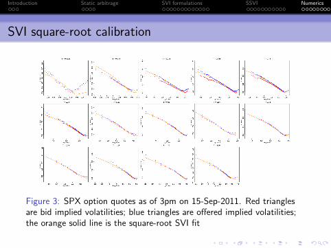
SVI square-root calibration

Figure 3: SPX option quotes as of 3pm on 15-Sep-2011. Red trianglesare bid implied volatilities; blue triangles are offered implied volatilities;the orange solid line is the square-root SVI fit


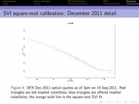
SVI square-root calibration: December 2011 detail

Figure 4: SPX Dec-2011 option quotes as of 3pm on 15-Sep-2011. Redtriangles are bid implied volatilities; blue triangles are offered impliedvolatilities; the orange solid line is the square-root SVI fit


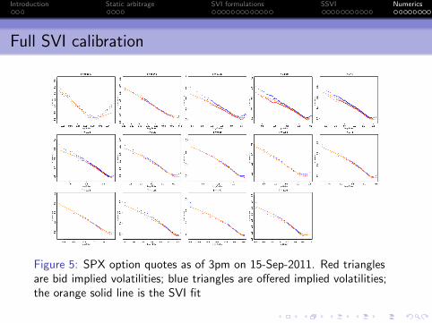
Full SVI calibration

Figure 5: SPX option quotes as of 3pm on 15-Sep-2011. Red trianglesare bid implied volatilities; blue triangles are offered implied volatilities;the orange solid line is the SVI fit


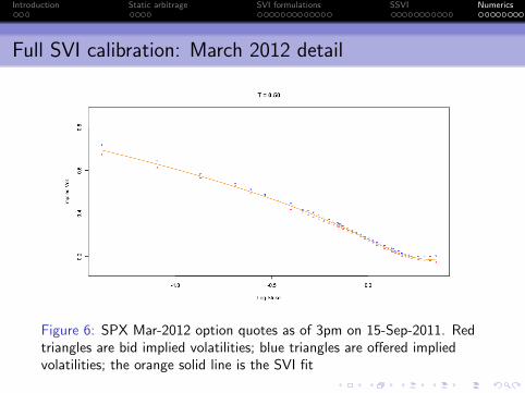
Full SVI calibration: March 2012 detail

Figure 6: SPX Mar-2012 option quotes as of 3pm on 15-Sep-2011. Redtriangles are bid implied volatilities; blue triangles are offered impliedvolatilities; the orange solid line is the SVI fit


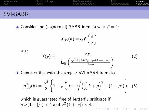
SVI-SABR

Consider the (lognormal) SABR formula with β = 1:

σBS(k) = α f

(k

α

)with

f (y) = − ν y

log

(√ν2 y2+2 ρ ν y+1−ν y−ρ

1−ρ

) . (2)

Compare this with the simpler SVI-SABR formula:

σ2BS(k) =

α2

2

{1 + ρ

ν

αk +

√( να

k + ρ)2

+ (1− ρ2)

}(3)

which is guaranteed free of butterfly arbitrage ifαν (1 + |ρ|) < 4 and ν2 (1 + |ρ|) < 4.


Butterfly arbitrage

It is well known that the SABR volatility smile is susceptibleto butterfly arbitrage.

The corresponding density is often negative for extreme strikes.

On the other hand, the SVI-SABR density is guaranteedpositive so long as αν t (1 + |ρ|) < 4 and ν2 t (1 + |ρ|) < 4.

Typical values of these parameters for SPX are ν2 t = 0.6,α = 0.2, ρ = −0.7 so for SPX there is empirically no butterflyarbitrage.SABR and SVI-SABR fit parameters are not identical but theyare similar.


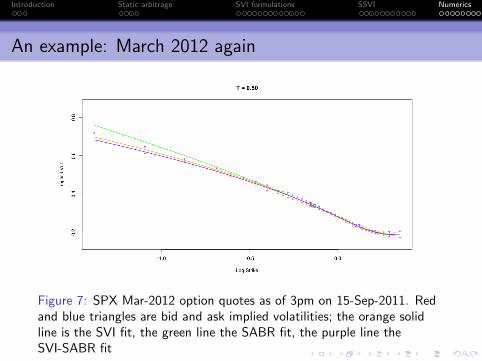
An example: March 2012 again

Figure 7: SPX Mar-2012 option quotes as of 3pm on 15-Sep-2011. Redand blue triangles are bid and ask implied volatilities; the orange solidline is the SVI fit, the green line the SABR fit, the purple line theSVI-SABR fit


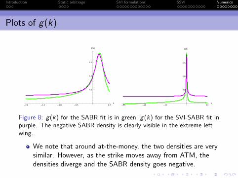
Plots of g(k)

-2.0 -1.5 -1.0 -0.5 0.5k

0.5

1.0

1.5

gHkL

-30 -20 -10 10k

0.5

1.0

1.5

gHkL

Figure 8: g(k) for the SABR fit is in green, g(k) for the SVI-SABR fit inpurple. The negative SABR density is clearly visible in the extreme leftwing.

We note that around at-the-money, the two densities are verysimilar. However, as the strike moves away from ATM, thedensities diverge and the SABR density goes negative.


Summary

We have found and described a large class of arbitrage-freeSVI volatility surfaces with a simple closed-formrepresentation.

Taking advantage of the existence of such surfaces, weshowed how to eliminate both calendar spread and butterflyarbitrages when calibrating SVI to implied volatility data.

We further demonstrated the high quality of typical SVI fitswith a numerical example using recent SPX options data.

Finally, we showed how a guaranteed arbitrage-free simple SVIsmile could potentially replace SABR in applications.


References

[1] Andreasen J., Huge B. Volatility interpolation, Risk, 86–89, March 2011.

[2] Carr, P., Wu, L. A new simple approach for for constructing implied volatility surfaces, Preprint available

at SSRN, 2010.

[3] Fengler, M. Arbitrage-free smoothing of the implied volatility surface, Quantitative Finance 9(4):

417–428, 2009.

[4] Gatheral, J., A parsimonious arbitrage-free implied volatility parameterization with application to the

valuation of volatility derivatives, Presentation at Global Derivatives, 2004.

[5] Gatheral, J., The Volatility Surface: A Practitioner’s Guide, Wiley Finance, 2006.

[6] Gatheral, J., Jacquier, A., Convergence of Heston to SVI, Quantitative Finance 11(8): 1129–1132, 2011.

[7] Gatheral, J., Jacquier, A., Arbitrage-free SVI volatility surfaces, SSRN preprint, 2012.

[8] Glaser, J., Heider, P., Arbitrage-free approximation of call price surfaces and input data risk,

Quantitative Finance 12(1): 61–73, 2012.

[9] Jackel, P., Kahl, C. Hyp hyp hooray, Wilmott Magazine 70–81, March 2008.

[10] Kahale, N. An arbitrage-free interpolation of volatilities, Risk 17:102–106, 2004.

[11] Lee, R., The moment formula for implied volatility at extreme strikes, Mathematical Finance 14(3):

469–480, 2004.

[12] Zeliade Systems, Quasi-explicit calibration of Gatheral’s SVI model, Zeliade white paper, 2009.

arbitrage-free svi volatility surfaces · introduction static arbitrage svi formulations ssvi...

Documents