NBER WORKING PAPER SERES

ARBITRAGE OPPORTUNITIES INARBITRAGE-FREE MODELS OF

BOND PRICING

David BackusSilverio Foresi

Stanley Zin

Working Paper 5638

NATIONAL BUREAU OF ECONOMIC RESEARCH1050 Massachusetts Avenue

Cambridge, MA 02138June 1996

We thank Fischer Black for extensive comments; Jennifer Carpenter, Vladimir Finkelstein, andBruce Tuckman for guidance on industry practice; Anthony Lynch for pointing out an error inan earlier draft; and Ned Elton for inadvertently initiating this project. Backus thanks theNational Science Foundation for financial support. This paper is part of NBER’s researchprogram in Asset Pricing. Any opinions expressed are those of the authors and not those of theNational Bureau of Economic Research.

O 1996 by David Backus, Silverio Foresi and Stanley Zin. All rights reserved. Short sectionsof text, not to exceed two paragraphs, may be quoted without explicit permission provided thatfull credit, including @ notice, is given to the source.

NBER Working Paper 5638June 1996

ARBITRAGE OPPORTUN~IES INARBITRAGE-FREE MODELS OF

BOND PNCING

ABSTRACT

Mathematical models of bond pricing are used by both academics and Wall Street

practitioners, with practitioners introducing time-dependent parameters to fit “arbitrage-free”

models to selected asset prices. We show, in a simple one-factor setting, that the ability of such

models to reproduce a subset of security prices need not extend to state-contingent claims more

generally. The popular Black-Derman-Toy model, for example, overprices call options on long

bonds relative to those on short bonds when interest rates exhibit mean reversion. We argue,

more generally, that the additional parameters of arbitrage-free models should be complemented

by close attention to fundamentals, which might include mean reversion, multiple factors,

stochastic volatility, and/or non-normal interest rate distributions.

David BackusStem School of BusinessNew York University44 West 4th StreetNew York, NY 10012-1126and NBER

Silverio ForesiStem School of BusinessNew York University44 West 4th StreetNew York, NY 10012-1126

Stanley ZinGraduate School of Industrial AdministrationCarnegie Mellon UniversityPittsburgh, PA 15213and NBER

1 Introduction

Since Ho and Lee (1986) initiated work on “arbitrage-free” models of bond pricing,

academics and practitioners have followed increasing] y divergent paths, Both groupshave the same objective: to extrapolate from prices of a limited range of assets ~he

prices of a broacler class of state-contingent claims. Academics study relatively parsi-monious models, whose parameters are chosen to approximate “average” or “typical”behavior of interest rates and bond prices. Practitioners, on the other hand, use

models with more extensive sets of time-dependent parameters, which they use toImatch current bond yields, and possibly other asset prices, exactly.

To practitioners, the logic of this choice is clear: the parsimonious models used byacademics are inadequate for practical use. The four parameters of the Vasicek ( 1977)and Cox-Ingersoll-Ross (1985) models, for example, can be chosen to match five points

on the yield curve (the four parameters plus the short rate), but do not reprodl~cr thecomplete yield curve to the degree of accuracy required by market participants. Evencomplex, multi-factor models cannot generally approximate bond yields with sufficient

accuracy. Instead, practitioners rely almost universally on models in the Ho and

Lee (1986) tradition, including those developed by Black, Derman, and Toy (1990),Black and ]{arasinski (1991), Cooley, LeRoy, and Parke (1992), Heath, Jarrow, and

Morton (1992), Hull and White (1990, 1993), and many others, Although analyticalapproaches vary across firms and even within them, the Black- DernlaI1-Toy model is

currently close to an industry standard.

Conversely, academics have sometimes expressed worry that the large parametf:rsets of arbitrage-free models may mask problems with their structure. A prominentexample is Dybvig (1989), who noted that the changes in parameter values required

by repeated use of this procedure contradicted the presumption of the theory thatthe parameters are deterministic functions of time. Black and Karasinski (1991, p 57)put it more colorfully: “When we value the option, we are assuming that its volatility

is known and constant, But a minute later, we start using a new volatility. Similarly,

we can value fixed income securities by assuming we know the one-factor short-rateprocess. A minute later, we start using a new process that is not consistent withthe old one, ” Dybvig argued that these changes in parameter values through time

implied that the framework itself was inappropriate.

We examine the practitioners’ procedure in a relatively simple theoretical setting,a variant of Vasicek’s (1977) one-factor C,aussian interest rate model that we refer

to as the benchmark theory. Our thought experiment is to apply models with time-

dependent drift and volatility parameters to asset prices generated by this theory. We

judge the models to be useful, in this setting, if they are able to reproduce prices of a

broad range of state-contingent claims. This experiment cannot tell us how well themodels do in practice, but it allows us to study the role of time-dependent parameters

in an environment that can be characterized precisely. VVefind, in this environment,that if the world exhibits mean reversion, then the use of time-dependent parametersin a model without mean reversion can reproduce prices of a limited set of assets,but cannot reproduce the prices of general state-contingent claims. In this sense,

these arbitrage-free ~models allow arbitrage opportunities: a trader basing prices on,

say, the Black- Derman-Toy model can be exploited by a trader who knows the tr~~e

structure of the economy.

A striking exalmple of misprizing in this setting involves options on long bonds,

Options of this type vary across two dimensions of time: the expiration date of theoption and the maturity of the bond on which the option is written. The Blacl<-

Dermall-Toy model has a one-dimensional array of volatility parameters that can be

chosen to reproduce either the prices of options with any expiration date on one-periodbonds or of options with common expiration dates on boncls of any maturity. But ifthe world exhibits mean reversion, this vector cannot reproduce the two-dimensional

array of prices of bond options. If the volatility parameters are chosen to match pricesof options on one-period bonds, then the model overprices options on long bonds.

While we think mean reversion is a useful feature in a model, it illustrates a

more general point: that misrepresentations of fundamentals, whatever their form,

cannot generally be overcome by adding arrays of time-dependent parameters. Fromthis perspective, the role of academic research is to identify appropriate fundamentals,

which might include multiple factors, stochastic volatility, and/or no~l-uormal interestrate movements. We conjecture that arbitrage-free models with inaccuracies along

any of these dimensions will misprice some assets as a result.

2 A Theoretical Benchmark

We use a one-factor Gaussian interest rate model as a laboratory in which to examinethe practitioners’ procedure of choosing time-dependent parameters to fit a bondpricing model to observed asset prices. The moclel is a close relative of Vasicek

(1977). Although in some respects it is simpler than those used by practitioners, itslog-linear structure is extremely useful in clarifying the roles played by its various

parameters.

2

To fix the notation, let ~ be the price at date t of a zero-coupon bond of maturity

71,the claim to one dollar at date t+ TL,By convention fi~= 1 (one dollar today costsone dollar). Bond yields are

y; = –n-l log b;

and forward rates are

f: = log(b;/b;+’). (1)

We label the short rate rt = Y; = f:.

We characterize asset prices in our benchmark theory, or laboratory, with a prici~~g

kerTLel: a stochastic process governing prices of state-contingent claims. Existence of

such a process is guaranteed in any arbitrage-free environment. We describe the kernelfor our theoretical environment in two steps. The first step involves an abstract statevariable z, whose dynamics follow

~t+l = pzt + (1 – p)6+ &t+l

—Zt +(1 —p)(J— ~t) +Et+l, (2)

with {Et} distributed normally and independently with mean zero and variance az.

The parameter y controls mean reversion: with y = 1 the state follows a random

walk, but with values between zero and one the conditional mean of future values ofz converges to the unconditional mean 6. Step two is the pricing kernel nt, which

satisfies– log ~n~+~= z~ + ~E~+I . (:3)

The parameter A, which we refer to as the price of risk, determines the covariance

between innovations to the kernel and the state and thus the risk characteristics ofbonds and related assets.

Given a pricing kernel, we derive prices of assets from the pricing relation

1 = Et(m~+~Rt+l), (4)

which holds for the gross return Rt+l on any traded asset. Since the one-period retllrnon an 71+ l-period bond is ~+1 /b~+l, the pricing relation gives us

(5)b:+l = Et(?7~t+l~;+l)7

which allows us to compute bond prices recursively, starting with the initial condition

b:=l.

Consider a one-period bond. From equation (5) and the initial condition L? = 1

we see that the price is the conditional mean of the pricing kernel: b: = Elnl,t+l.

3

Since the kernel is conditionally lognormal, we need the following property of log-normal random variables: if log x is normal with mean p and variance az, thenlog E(x) = p + 02/2. From equation (3) we see that log ?n~+l has conditional mean

–zt and conditional variance (Aa)2. Thus the one-period bond price satisfies

log b; = –2, + (Aa)2/2

and the short rate isr~ = –logb; = z~ – (Aa)2/2.

Thus the short rate ~ is the state z with a shift of origin. The mean

6 – (Ao)2/2, which we denote by L in the rest of the paper.

The stochastic process for z, equation (2), implies similar behavior

rate:

rt+l = Tt+(1 –~)(p–

a discrete time version of Vasicek’s (1977) shortshort rate are

for n >1, which yields conditional first and

E,(r,+n) = l-, + (1

and w

Tt) + Et+l,

rate diffusion. Future

n

second moments of

– 9“)(P – ~t)

j=l

We return to these formulas later.

Prices of long bonds follow from (5);properties are conveniently summarized

of the short rate:

(6)

short rate is

for the short

values of ~;~

(8)

(9)

details are provided in Appendix A.1. Theirby forward rates, which are linear functions

[ ( 1;:)2]a,2,f;=rt+(l –w’’)(p–rt)+ A2– A+ (lo)

for all T1~ O. Given forward rates, we can compute bond prices and yields from theirdefinitions, The right side of equation (10) has a relatively simple interpretation, If

we compare it to (8), we see that the first two terms are the expected short rate r~periods in the future. We refer to the last term as a risk premium and note that it

4

depends on three parameters: the magnitucleof risk (o), the price of risk (A), and

mean reversion (y).

Both the Ho and Lee (1986) and Black, Derman, and Toy (1990) models arecapable of reproducing an arbitrary forward rate curve (equivalently, yields or bond

prices), including one generated by a theoretical model like this one, An issue weaddress later is whether this capability extends to more complex assets, With thisin mind, consider a European call option at date t, with

strike price k, on a zero-coupon bond with maturity n

lognormality of bond prices in this setting, the call price is

(1973) formula,T,n

Ct = b;+”N(dl) – kb:fv(~2),

where N is the cumulative normal distribution function,

~ _ log[b:+n/(b:k)] + v;,n/2l—

and the option volatility is

expiration date t + ~ andat expiration. Given thegiven by the Blacl<-Sc.holes

(11)

(12)

See Appendix A.4. .Jamshidian (1989) reports a similar formula for a continuous-ti]ne

version of the Vasicek model. The primary difference from conventional applicationsof the Black-Scholes formula is the role of the mean reversion parameter ~ in ( 12).

3 Parameter Values

We are trying, in this paper, to make a theoretical point, but we find it useful to

illustrate the theory with numerical examples. The parameter values come from

an informal moment matching exercise based on properties of monthly yields for

[JS government securities computed by McCullocb and Kwon ( 1993). Some of theproperties of these yields are reported in Table 1 for the sample period 1982-91,

We choose the parameters to approximate some of the salient features of bondyields using a time interval of one month. From equation (7) we see that ~ is theunconditional mean of the short rate, so we set it equal to the sample mean of the

5

one-month yield in Table 1, 7.483/1200. (The 1200 converts an annual percentagerate to a monthly yield. ) The mean reversion parameter y is the first autocorrelationof the short rate. In Table 1 the autocorrelation is 0,906, so we set y equal to this

value. This indicates a high degree of persistence in the short rate, but less than with

a random walk. The volatility parameter a is the standard deviation of innovationsto the short rate, which we estimate with the standard error of the linear regression

(7). The result is a = 0.6164/1200. Thus the values of (p, O, p) are chosen to matchthe mean, standard deviation, and autocorrelation of the short rate. We choose the

final parameter, the price of risk A, to approximate the slope of the yield curve. Note

from (10) that mean forward rates, in the theory, are

This tells us that to produce an increasing mean forward rate curve (implying anincreasing mean yield curve) we need A to be negative. The price of risk parameter,in other words, governs the average slope of the yield curve. One way of fixing A, thent

is to select a value that makes the theoretical mean yield curve similar to the samplemean yield curve, given our chosen values for the other three parameters. An example

is pictured in Figure 1, where ~vesee that A = —750 produces theoretical mean yields(the line in the figure) close to their sample means (the stars) for maturities between

one month and ten years. With more negative values the mean yield curve is steeper,and with less negative (or positive) values the yield curve is flatter (or downwardsloping).

Thus we see that all four parameters are required for the theory to imitate thedynamics of interest rates and the average slope of the yielcl curve. We use thesebenchmark values later to illustrate differences in prices across bond pricing models.

4 Ho and Lee Revisited

We turn now to the use of time-dependent parameters to fit theoretical models to

observed asset prices. We apply, in turn, analogs of the models of Ho and Lee ( 1986)and Black, Derman, and Toy (1990) to a world governed by the benchmark theory of

Section 2.

Our first example is a (;aussian analog of Ho and Lee’s (1986) binomial interestrate model. The analog starts with a state equation,

6

with time-dependent parameters {CYt} and normally and independently distributed

innovations {qt} with mean zero and constant variance 92. The pricing kernel is

– log T?lt+l = ~t + 7TL+1. (14)

lVe use different letters for the parameters than in the benchmark theory to indicatethat they may (but need not ) take on different values, Our Ho and Lee analog differsfrom the benchmark theory in two respects, First, the short rate process does notexhibit mean reversion, which we might think of as setting ~ = 1 in equation (2).

Second, the state equation (13) includes time-dependent “drift” parameters {at}.

Given equations (13,14), the pricing relation (5) implies a short rate

and forward rates

(15)j=l

for rZ~ 1. See Appendix A.2, Note that (10) differs from (15) of the benchmark intwo ways. One is the impact of the short rate on long forward rates. A unit increase

in r is associated with increases in f“ of one in Ho and Lee, but (1 — pn) < 1 in the

benchmark. The other is the risk premium, the final term in ecluation (1,5).

Despite these differences, time-dependent drift parameters allow the Ho and Leemodel to reproduce some of the features of the benchmark theory. One such feature

is the conditional mean of future short rates. The future short rates implied by thismodel are .

which implies conditional means of

71

Et(rt+n) = ~t + ~ ~t+j (17)j=l

for 71>0. If we compare this to the analogous expression for the benchmark theory,equation (8), we see that the two are equivalent if we set

n

(18)

7

Thus the time-dependent drift parameters of the Ho and Lee model can be chosen toimitate this consequence of mean reversion in the benchmark theory.

In practice it is more common to use the drift parameters to fit the model to the

current yield curve. To fit forward rates generated by the benchmark theory we need[compare (10,15)]

5 at+j = (1 -~’’)(p -r,) + [A’ - (A+(l -~’L)/(l -~))’] cJ2/2j=l

- [72 - (7+ ~)’] P2/2 (19)

The drift parameters implied by (18) and (19) are, in general, different. Since

we can equate the two expressions when y = 1 by setting ~ = a and ~ = J. But

when O < v < 1 the two expressions cannot be reconciled. This is evident in Figure 2,where we graph the two choices of cumulative clrift parameters, ~~=1 a~+j, using the

parameters estimated in Section 3, with ~ = a, ~ = A, and r = 3.0/1200. The drift

parameters that reproduce the conditional mean converge rapidly as the effects of

mean reversion wear off. But the drift parameters that fit the current yield curve getsteadily smaller as they offset the impact of maturity on the risk premium in this

model. This results, for the range of maturities in the figure, in a declining termstructure of expected future short rates, while the benchmark implies the reverse,

The discrepancy in the figure between the two choices of drift parameters is aconcrete example of

Remark 1 The parameters of the Ho and Lee model can be chose~t to match the

current yield curve, or the conditio~tal means of future short ratesj bllt they ca~l~lot

ge~lerally do both.

This property of the Ho and Lee model is a hint that time-dependent drift parametersdo not adequately capture the effects of mean reversion in the benchmark theory.Dybvig (1989, p ,5) makes a similar observation. A closer look indicates that thedifficulty lies in the nonlinear interaction in the risk premium between mean reversionand the price of risk. In the benchmark theory, the risk premium on the ~~-period

forward rate [see equation (10)] is

8

In the Ho and Lee model, equation (15), the analogous expression is

If we choose ~ = A and ~ = a the two expressions are equal for ~1= 1, but they move

apart as 71grows. The discrepancy noted in Remark 1 is a direct consequence.

A similar comparison of conditional variances also shows signs of strain. Theconditional variances of future short rates implied by the Ho and Lee model are

Vart(rt+m) = n~z.

If we compare this to the analogous expression in the benchmark theory, equation (9),we see that they generally differ when ~ # 1. With y < 1 and ~ = CJ,the conditionalvariances are the same for n = 1, but for longer time horizons they are greater in the

Ho and Lee model. We summarize this discrepancy in

Remark 2 The parameters of the Ho and L~e model cannot be chosc:u to re])roduce

the conditional variances of future short rates.

Thus we see that additional drift parameters allow the Ho and Lee model to

imitate some of the effects of mean reversion on bond yields. They cannot? however,reproduce the conditional variances of the benchmark theory, Dybvig (1989, p 5)summarized this feature of the Ho and Lee model more aggressively: “[T]he Ho

and Lee model starts with an unreasonable implicit assumption about innovations in

interest ratesj but can obtain a sensible initial yield curve by making an unreasonableassumption about expected interest rates. lJnfortunately, while this ,.. give[s] correct

pricing of discount boncls..., there is every reason to believe that it will give illcorrertpricing of interest rate options. ” Dybvig’s intuition about options is easily verified.The Black- Scholes formula, equation (11), applies to the Ho and Lee model if we useoption volatility

v; ~ = Var,(log b~+~) = ~(n~)’. (20)This formula cannot be reconciled with that of the benchmark theory, equation ( 12),for all combinations of ~ and n unless y = 1. If we choose the volatility parameter~ to reproduce the option volatility ZJI,Iof a short option on a short bond, then

we overstate the volatilities of long options on long bonds. As a result, the modelovervalues options with more clistant expiration dates ancl/or longer underlying bonds.

We see in Figure 3 that call prices CTI1implied by the Ho and Lee model canbe substantially higher than those generated by the benchmark theory. The figure

9

expresses the rnispricing as a premium of the Ho and Lee price over the price generated

by the benchmark theory. Benchmark prices are based on the parameter values of

Section 3. Ho and Lee prices are based on drift parameters that match current bondprices, equation (19), and a volatility parameter p = a that Imatcbes the optionvolatility VI,1 of a one-period option on a one-period bond. Both are evaluated at

strike price k = bj/bJ+”. For ~ = 1 the two models generate the same call price, but

for options with expiration dates 12 months in the future the Ho and Lee price ismore than ,50 percent higher.

5 Black, Derman, and Toy Revisited

Black, Derrnan, and Toy ( 1990) extend the time-dependent parameters of Ho and

Lee to a second dimension. They base bond pricing on a binomial process for thelogarithm of the short rate in which both drift ancl volatility are tilne-(le~]elldetlt.

We build an analog of their model that retains the linear, Gaussian structure ofprevious sections, but includes these two sets of time-dependent parameters. Givena two-parameter distribution like the normal, time-dependent drift and volatility can

be used to match the conditional distribution of future short rates exactly and thusto mitigate the tendency of the Ho and Lee model to overprice long options. The

question is whether they also allow us to reproduce the prices of other interest-rate

derivative securities.

Our analog of the Black-Derman-Toy model adds time-dependent volatility to thestructure of the previous section: a random variable z follows

Zt+l = ~t + ~t+l + qt+l (21)

and the pricing kernel is

– log ?n~+~= z~ + yqt+~ . (22)

The new ingredient is that each qt has time-dependent variance ~~~. This structurediffers from the benchmark theory in its absence of mean reversion (the coefficient of

one on zt in the state equation) and in its time-dependent drift (the CY’S)and volatility(the ~’s).

We approach bond pricing as before. We show in Appendix A.2 that the shortrate is

r~ = – log (EtT?z~+~)= z~ – (~pt+~)2/2

10

and forward rates are

for 71~ 1. Equation (23) reduces to the Ho and Lee expression, equation (15), when

@t = @ for all t. AS in the Ho and Lee model, forward rates differ from the benchmarkin both the impact of short rate movements on long forward rates and the form of

the risk premium.

We can use both sets of time-dependent parameters to approximate asset prices

in the benchmark theory. Consider the conditional distribution of future short rates.The short rate follows

so future short rates are

Their conditional mean and variance are

Et(rt+n) = ~t + 72(P?+l–P:+,z+l)/2 +fat+,j=l

This model, in contrast to Ho and Lee, is able to match the conditional variancesof the benchmark theory, which we do by choosing volatility parameters that declinegeometrically:

This implies conditional variances of

the same as ecluation (9) of the theory. Similar patterns of declining time-dependentvolatilities are common when these methods are used in practice, Black, Derman, and

11

Toy’s numerical example included (see their Table I). To match the conclit ional mean

of the benchmark theory, equation (8), we choose drift parameters that satisfy

Thus we see, as Black, Derman, and Toy (1990, p :33) suggest, that we can fit the

first two moments of the short rate with two “arrays” of parameters:

Remark 3 The parameters of the Black-Derman-Toy model caTl bc chosen to repro-

duce the conditional means and variances of future short rates.

Given the critical role played by volatility in pricing derivative assets, this representsan essential advance beyond Ho and Lee.

Despite time-dependent volatility parameters, the model cannot simultaneo~lslyreproduce the conditional moments of the short rate and the forward rates of thebenchmark theory. The drift parameters that reproduce the forwarcl rate curve,equation (10), are

= (1 - pn)(p - r,)+ [A’ -(A+ (1 - y“)/(1 - y))’] 0’/2j=]

Comparing (28)

the difference in

and (29) we see that the two are not equivalent, in general. ii~e note

Remark 4 Give71 volatility parameters (27) that reproduce the conditional variaTlcesof future rates, the drift parameters of the Black- Derman-Toy model can be choserl

to match the current yield curve, or the conditioltal means of future short rate.~, but

they cannot generally do both.

Figure 4 plots the difference between (29) and (28). The parameter values are thoseof Section 3, with ~ = A, p~+j = y ~–la, and r = ;3.()/12()(). The differences are smaller

than those of Figure 2 for the Ho and Lee model, but are nonzero nonetheless.

Remark 4 is a hint that the Black-Dermall-Toy analog cannot generate accurate

prices for the full range of state-contingent claims in the benchmark economy, but we

12

can see this more clearly by looking at specific assets. Consider European call optionson zero-coupon bonds. Once more the lognormal structure of the model means thatthe Black- Scholes formula, equation (11), applies. If we choose drift parameters to fit

the current yield curve, then any difference between call prices in the model and thebenchmark theory must lie in their option volatilities. The option volatility for the

Black-Derman-Toy analog is

V;,l= ‘n2 ~ ~~+j.

j=l

see Appendix A.4. If we restrict ourselves to options on one-period bonds (so that71= 1), we can reproduce the volatilities of our theoretical environment by choosing~6’s that decline geometrically with time, the same choice that replicates COI]ditionalvariances of future short rates, equation (27).

However, the Black- Dermal~-Toy analog cannot simultaneously reproduce pricesof options on bonds of longer maturities. If we use the geometrically declining pa-

rameters of equation (27), the option volatility is

From (12) we see that the ratio of option volatilities is

BDT Volatility nz

Benchmark Volatility = (1 + ~ + . + ~“-l)z

This ratio is greater than one when O < w <1 and n > 1, and implies that when theBlacl~-Dernlall-Toy analog prices options on short bonds correctly, it will overpriceoptions on long bonds. We see in Figure 5 that this rnispricing gets worse the longer

the maturity of the bond, and is greater than 150 percent for bonds with maturities

of two years or more. As in Figure 3, benchmark prices are based on the parametersof Section 3, the drift parameters of the Black- Dernlall-Toy analog are chosen to

reproduce the current yield curve, the strike price is k = b~/b~+”, and the expirationperiod is r = 6. Thus we have

Remark 5 The parameters of the Black-Derman-Toy model cannot

prices of call options o~t bonds for all maturities a~ld expiration dates.

The difference in option volatilities, and hence in call prices, between the twomodels stems from two distinct roles played by mean reversion in determining prices

13

of long bonds. Mean reversion appears, first, in the impact of short rate innovationson future short rates. We see from (9) that the impact of innovations on future short,

rates, in the theory, decays geometrically with the time horizon ~, This feature is

easily mimicked in the Black-Dernlan-Toy model, as we have seen, by using volatilityparameters {~f} that decay at the same rate. The second role of mean reversionconcerns the impact of short rate movements on long bond prices. In the Black-

Dermall-Toy model, a unit decrease in the short rate results in an 71unit, increase inthe logarithm of the price of an ~~-period bond; see Appendix .4.2. In the benchmark

theory, the logarithm of the bond price rises by only (I+p+. ~.+p’’-’) = (1–p’’)/(l –y); see Appendix Al. This attenuation of the impact of short rate innovations on long

bond prices is a direct consequence of mean reversion. It is not, however, reproducedby choosing geometrically declining volatility parameters and is therefore missing fromcall prices generated by the Black- Derman-Toy analog. Stated somewhat differently:

the Black- Derman-Toy analog does not reproduce the hedge ratios of the benchmarl{theory.

As a practical matter, then, we might expect the Blat.k-Dernlall-Toy procedure to

work well in pricing options on short term instruments, including interest rate caps.For options on long bonds, however, the model overstates the option volatility and

hence the call price. A common example of such an instrument is a callable bond.This procedure will generally overstate the value of the call provision to the issuer,

in the theoretical environment, and thus understate the value of a callable long-termbond.

The discrepancy between option prices generated by the benchmark theory and

the Black-Dernlan-Toy analog illustrates one difficulty of using models with tinle-

dependent parameters: that a one-dimensional vector of time-dependent volatilityparameters cannot reproduce the conditional variances of bond prices across the two

dimensions of maturity and time-to-expiration. We turn now to a second example ofmisprizing: a class of “exotic.” derivatives whose returns display different sensitivitythan bonds to interest rate movements,

Consider an asset that delivers the power O of the price of an n-period bond oneperiod in the future. This asset has some of the flavor of derivatives with magnified

sensitivity to interest rate movements made popular by Bankers Trust, yet ret sinsthe convenient log-linearity of bond prices in our framework. As with options, wecompare the prices implied by the benchmark theory,

log ~ = - (.,+ (Aa)2/2) +Hlogb;+(’+’11::)2a2’2

–@(l–pn)(p– r,), (30)

14

with those generated by the Black- Derman-Toy analog,

n

–6’ ~ [(n– j)(~t+j+l – Qt+j ) -(~+ n - j)2(P?+j+l - Pt+j)2/2] - (31)j=l

Both follow from pricing relation (4) with the appropriate pricing kernel.

Suppose we choose the parameters of the Black-Dernlall-Toy analog to ulatchthe conditional variance of future short rates [equation (26)], the current, yield curve[equation (29)], and the price of risk [y = A]. ~~an this model reproduce the prices ofour exotic asset for all values of the sensitivity parameter 9? The answer is generally

no. When n = 1 the two models generate the same price d) for all values of H,just aswe saw that the two sets of cumulative drift parameters were initially the same (see

Figure 4 and the discussion following Remark 4). For longer maturities, however, theprices are generally different. Figure 6 is an example with 7Z= 60 and r = ~3.00/1200.

We see that for values of O outside the unit interval, the Black-Dermall-Toy analogoverprices the exotic, although the difference between models is smaller than foroptions on long bonds. Thus

Remark 6 The parameters of the Black-Derman-Toy model can be chosrn to match

both the current yield curve and the term structure of volatility for options ort onc-

period bonds, but they cannot generally replicate the prices of more exotic derivatives.

These examples of rnispricing illustrate a more general result: that the Blacl<-Dermall-Toy analog cannot replicate the state prices of the benchmark theory. This

result is stated most clearly using stochastic discount factors,

which define n-period-ahead state prices. We show in the Appendix that the benchm-

ark theory implies discount factors

and the Black- Derman-Toy analog implies

15

As long as y # 1 and a # O, the seconcl expression cannot be made e(luiva]ent to the

first:

Proposition 1 The time-depende.?lt dTift an,d volatility parameters of th~ Black-Dcr-

ma?t-Toy model cannot be chosen to reproduce the stochastic discount factors of th~

benchmark theory.

A proof is given in Appendix A.3. The difficulty lies in the innovations,

There is no choice of volatility parameters {@t} in Blaclt-Dernlall -Toy that can repli-cate the nonlinear interaction of mean reversion (y) and the price of risk (A) in the

benchmark theory.

In short, the time-dependent drift and volatility parameters of a model like the

Black-Derman-Toy analog cannot replicate the prices of derivative assets generated

by a model with mean reversion.

6 Arbitrage and Profit Opportunities

In the laboratory of the benchmark theory, the Black-Dermall-Toy analog systenlati-

cally misprices some assets. In this section we consider strategies that might be usedto profit from traders using prices indicated by the Black-Dermall-Toy model.

One way to exploit someone trading at Black-Derman-Toy prices is to arbitragewith someone trading at benchmark prices. If, as we have seen, a Black- Dern~all-

Toy trader overprices options on long bonds relative to those on short rate, and abenchmark trader does not, then we can buy frolm the latter and sell to the former,

thus making a riskfree profit. This is as clear an example of arbitrage as there is. Blltsince such price differences are so obvious, they are unlikely to be very common.

It is less easy to exploit a Black-Derman-Toy trader when trades take place onlyat prices dictated by the model. Since Black- Derman-Toy prices are consistent witha pricing kernel, they preclude riskless arbitrage. We can often devise, however, dY-

namic strategies whose returns are large relative to their risk. One sllch strategy

16

involves call options on long bonds, which (again) the Black- Dernlall-Toy model gel]-erally overvalues. If we sell the option to the trader at date t,and liquidate at t + 1,

we might expect to make a profit. This seems particularly likely in the option’s final

period, since the option is overvalued but the bonds on which the option is writtenare not.

Before we evaluate this strategy, we need to explain how the Blacl~-Dernlal] -Toy

trader prices assets through time. .4 trader using the Black-Dermall-Toy model gel]-

erally finds, both in practice and in our theoretical setting, that the t,iI~le-del]ell(ielltparameters must be reset each period. In our setting, suppose the trader choosesvolatility parameters at date t to fit implied volatilities from options on short bonds.

As we have seen, this leads her to set {~~~+1,~t+z, ~t+3, . .} eclual to {a, pa, y20, . . .}.

If the parameters were literally time-dependent, then in the following period logic dic-

tates that we set {~~+2, ~t+3, /~~+4,. . .} equal to {pa, V2a, W30, . .}. But if we calibrateonce more to options on one-period bonds, we would instead use {cJ, pa, ~2a, .}.This leads to a predictable upward jump in the volatility parameters from one pe-

riod to the next, as in Figure 7. Similarly, the drift parameters must be adjusted

each period to retain the model’s ability to reproduce the current yield curve, Thesechanges in parameter values through time are an indication that the model is im-

perfectly imitating the process generating state prices, but they nevertheless improve

its performance. In this sense the internal inconsistency noted by Dybvig (1989) is asymptom of underlying problems, but not a problem in its own right. Thus our trader

prices call options using drift and volatility parameters that match, each period, theyield curve and the term structure of volatilities impliecl by options 011 one-periodbonds, equations (29) and (27), respectively.

Now consider a strategy against such a trader of selling a ~-period option on an

~t-period bond and buying it back one period later. The gross one-period return fromthis strategy is

Rt+l = –c;;;’’’/c;’n,

for r z 1, with the convention that an option at expiration has value c~)” = (~ – k)+.

The profit from this strategy is not riskfree, but it can be large relative to the riskinvolved. In the world of the benchmark theory, the appropriate adjustment for riskis given by the pricing relation (4). We measure the mean excess risl{-adjusted return

bya = E (7nt+l Rt+l) — 1,

using the pricing kernel nt for the benchmark economy. This measure is analogolls to

Jensen’s alpha for the CAPNI and is the appropriate risk adjustment in this setting.For the trading strategy just described, and the parameter values of Section :3, the

returns are in the neighborhood of several hundred percent per year; see Figurt~ 8.

17

The returns in the figure were computed by .Monte Carlo, and concern two-period(~=2) options on bonds for maturities (n) between 1 and 24 months. The returns are

greater with ~ = 1, but decline significantly as ~ increases. For ~ >6 the overpricing

is difficult to exploit, since the overpricing of a five-period option the following period

is almost as great.

7 Mean Reversion and Other Fundamentals

We have seen that the time-dependent drift and volatility parameters of analogs ofthe Ho and Lee (1986) and Black- Dermall-Toy (1990) models cannot reproduce the

prices of state-contingent claims generated by a model with mean reversion. Thisthought experiment does not tell us how well these models perform in practice, but

it indicates that extra parameters are not a solution to all problems: they need to b~used in the context of a structure with sound fundamentals.

We focused on mean reversion because we find it an appealing feature in a bond

pricing model, yet it is missing from the most popular binomial interest rate mod-els. The estimated autocorrelation of 0.906 reported in Table 1 is not substantially

different from one, but a value of one has, in the benchmark theory, two apparentlycounterfactual implications for bond yields, The first is that the mean yield curve

eventually declines (to minus infinity) with maturity. In fact yield c,urves are, on

average, upward sloping, Figure 1 being a typical example. A second implicationwas pointed out by Gibbons and Ramaswamy (1993) and may be more telling: with

y close to one, average yield curves exhibit substantially less curvature than we seein the data. .An example with p = 0.99 is pictured in Figure 9, where we have setA = –200 to keep the theoretical 10-year yield close to its sample mean. These two

implications illustrate the added power of combining time-series and cross-section

information, and suggest to us that random walk models overstate the persistenceof the short-term rate of interest. For these reasons, we feel that mean reversion issuggested by the properties of bond prices.

For similar reasons, Black and l{arasinski (1991), Heath, Jarrow, and h’Iorton(1992), and Hull and White (1990, 1993) have developed ways of introducing mea~~-reversion into arbitrage-free models. Despite these developments? mean reversion is

generally ignored by all but the most sophisticated market participants. Financial

professionals do not generally reveal their methods, but they can be inferred frol~~other sources. One source is books on fixed income modeling. Tuckman ( 1995) isaimed at quantitatively-oriented MBA students and is used in Salomon Brothers’

18

sales and trading training course, yet devotes only four pages to models with mean

reversion. Sundaresan ( 1996) targets a similar audience and disregards mean reversion

altogether. Perhaps a better source is Bloomberg, the leading purveyor of fixedincome information services. Calculations on Bloomberg terminals of the “fair value”of interest rate derivatives are based on a log-normal analog of the Ho and Lee model,and calculations of “option-adjusted spreads” for callable bonds use the same model

as the default (Bloomberg 1996), with Black, Derman, and Toy (1990) and Hull and

White (1990) available as alternatives.

However, we think the central issue is not, mean reversion, but whether pricingmodels — arbitrage-free or not — provide a good approximation to the fundanlell-tals driving bond prices. Mean reversion, in this context, is simply an example of

a fundamental that cannot be mimicked by time-dependent drift and volatility pa-rameters. A second example is multiple factors. Work by, among others, Brennauand Schwartz (1979), Chen and Scott (1993), Duffie and Singleton (1995), Dybvig

(1989), Garbade (1986), Litterman and Scheinkman (1991), and Stambaugh (1988)clearly indicates the benefits of additional factors in accounting for the evolution of

bond prices through time, Longstaff and Schwartz (1992) are representative of agrowing number of studies that identify a second factor with volatility, whose varia-

tion through time is apparent in the prices of options on fixed income instruments.

Yet another example is the fat tails in weekly interest rate changes documented byDas (1994), who introduced jumps into the standard diffusioll-basecl models, Wewould guess that models that ignore any or all of these fundamentals will, as a direct

consequence, produce inaccurate state prices.

We argue, in short, that fundamentals matter, and that poor choice of fundanlell-

tals cannot generally be rectified by judicious use of time-depenclent parameters.

8 Final Thoughts

We have examined the practitioners’ methodology of choosing time-dependent pa-rameters to fit an arbitrary bond pricing model to current asset prices. We showed,in a relatively simple theoretical setting, that this method can systematically mis-price some assets. Like Ptolemy’s geocentric model of the solar system, these models

can generally be “tuned” to provide good approximations to (in our case) prices ofa limited set of assets, but they may also provide extremely poor approximations forother assets. As Lochoff (1993, p 92) puts it: ‘LEven bad models can be tuned to givegood results” for simple assets.

19

Whether these theoretical examples of misprizing can be used to direct tradingstrategies in realistic settings depends on the relative magnitudes of the misprizing

and the inevitable approximation errors of more parsimonious models. We would not

be willing, at present, to bet our salaries on our benchmark theory. Nevertheless, wethink the exercise indicates that it is important to get the fundamentals right. In ourthought experiment, fundamentals were represented by the degree of mean reversionin the short rate, and we saw that a mistake in this dimension could lead to large

pricing errors on some securities. The extra time-dependent parameters, in other

words, are not a panacea: they allow us to reproduce a subset of asset prices, but do

not guarantee accurate prices for the full range of interest-rate derivative securities.In more general settings, we expect a model with 71arrays of parameters to be able to

reproduce the term structure of prices of rt classes of assets, but if the fundamentalsare wrong there will be some assets that are mispriced.

The difficulty in practice is that even the best fundamental models provide only

a rough approximation to the market prices of fixed income derivatives. That leaves

us in the uncertain territory described by Black and Karasinski (1991, p 57): “[~>ne]approach is to search for an interest rate process general enough that we can assume

it is true and unchanging. ... While we may reach this goal, we don’t know enough touse this approach today. ” Best practice, we think, is to combine current knowledge

of fundamentals with enough extra parameters to make the approximation adequate

for trading purposes.

20

A Mathematical Appendix

W’e derive many of the formulas used in the text. For both the benchmark theoryand our analog of the Black-Derman-Toy modelt we derive the stochastic discount

factors implied by the pricing kernels listed in the text, and the implied bond prices,forward rates, and prices of call options on discount bonds. The result is effectively

a mathematical summary of the paper.

A.1 Benchmark Theory

We characterize bond pricing theories with stochastic cliscount factors,

or —log ~ft,t+~, = – ~;=l log nLt+j. Given the pricing kernel ~n of our benchmark

theory [equations (2) and (3)], the stochastic discount factors are

for n z 1. Given the discount factors, we compute bond prices from fi~ = EtIWt,~+,Z[a consequence of (5)]:

–log~ = nd+

Forward rates [see (1)] are

l–~” 2A+— n2/’2,

l–p

which includes a short rate of rt = j: = Zt – (Aa)2/2.

It is conventional to express discount factors, bond prices, and forward rates in

terms of the observable short rate T rather than the abstract state variable z, which

21

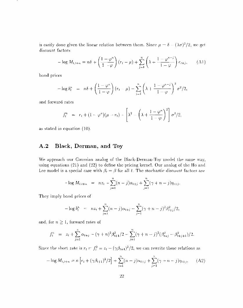
is easily done given the linear relation between them. Since p = 6 — (~a)z/2, we getdiscount factors

bond prices

and forward rates

as stated in equation (10)

A.2 Black, Derman, and Toy

We approach our Gaussian analog of the Black-Dern~an-Toy model the salne way,using equations (21 ) and (22) to define the pricing kernel. Our analog of the Ho andLee model is a special case with ,Bt= ~ for all t. The stochastic discount factors are

They imply bond prices of

71

– log b: = nzt + ~(n — j)at+j — ~(v + n - j)2Pt+j/2j=l j=l

and, for n 2 1, forward rates of

Sillce the, short rate is ~t = ~~ = Zt — (y@t+l )2/2, we can rewrite these relations as

22

and

as stated in equation (23). With,flt+j= P thisreducesto

equation (15) of the Ho and Lee model.

A.3 Nonequivalence of Discount Factors

Our examples of assets that are mispriced by the Black-Dernlall-Toy model indicatethat E31ack-Derman-Toy cannot generally reproduce the stochastic discount factors of

our benchmark theory:

Proposition 1 The parameters {y, at, Pt} Of the Black-DermaTl-Toy model CUILILOi

be chosen to reproduce the stochastic discount factors of the benchmark theory.

The proof consists of comparing the two discount factors, (A 1) for the benchmarktheory and (A2) for the Black-Derma~l-Toy model. The deterministic terms of (,41)

and (A2) are relatively simple. For, say, the first n discount factors, we can equate

the conditional means of (Al) and (A2) by judicious choice of the n drift parameters

{~t+l,~~~,Q,+,,}. The stochastic terms, however, cannot generally be ecluated. We

can represent the initial stochastic terms for the benchmark theory in an array likethis:

j=l j=z j=~

n=l ~ct+l

n=z (A+ l)Et+, A&t+2?1= :3 (A+ 1 + y)&t+, (A+ l)&,+2 AE~+~

23

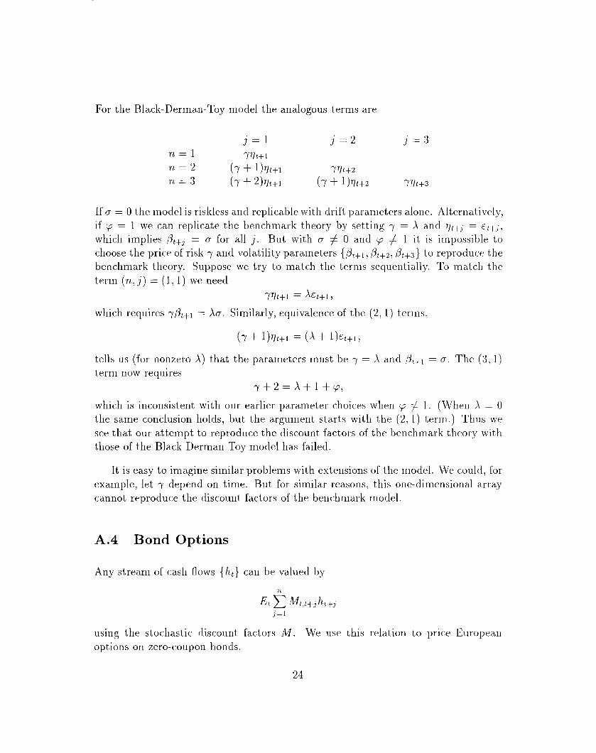
For the Black-Derman-Toy model the analogous terms are

j=l j=~ j=:~

n=l 7qt+lTL=z (7+ I)?/t+] yvt+2

n=~ (7+ ~)qt+l (7+ 1 )qt+2 ‘i7t+3

If a = Othe model is riskless and replicable with drift parameters alone. Alternatively,if p = 1 we can replicate the benchmark theory by setting ~ = ~ and T~~+j= ct+i,

which implies ~t+i = a for all j. But with a # O and v # 1 it is impossible tochoose the price of risk y and volatility parameters {~t+l, ~t+2, ~t+3} to reproduce thebenchmark theory. Suppose we try to match the terms sequentially. To match the

term (n, j) = (1,1) we need

~~t+l = ~&t+l,

which requires ~~t+l = ~0. Similarly, equivalence of the (2, 1) terms,

(7+ l)qf+l = (~+ l)~t+l,

tells us (for nonzero A) that the parameters must be ~ = A and ~~~+1= a. The (13,1)

term now requiresy+2=A+l+y,

which is inconsistent with our earlier parameter choices when y # 1. (When A = Othe same conclusion holds, but the argument starts with the (2, 1) term.) Thus we

see that our attempt to reproduce the discount factors of the benchmark theory with

those of the Black-Dermall-Toy model has failed.

It is easy to imagine similar problems

example, let ~ depend on time. But for

cannot reproduce the discount factors of

A.4 Bond Options

with extensions of the model. We could, for

similar reasons, this one-dimensional array

the benchmark mode].

Any stream of cash flows {ht} can be valued by

?Z

j=l

using the stochastic discount factors M. We use

options on zero-coupon bonds.

this relation to price European

24

Consider a European call option at date t with expiration date t + ~. The optiongives its owner the right to buy an n-period bond at date t + T for the exercise pricek, thus generating the cash flow

h ,+, = (b;+. - ~)+,

where x+ = max{O, x} is the nonnegative part of ~. The call price is

“n = E, [Mt,t+,(v+.– ~)+]Ct (A3)

Computing this price involves evaluating (A3) with the appropriate discount factorand bond price.

Both of our theories have lognormal discount factors and bond prices, so to

evaluate ( A3) we need two properties of lognormal expectations, Let us say that

log z = (log xl, log Zz) is bivariate normal with mean vector p and variance matrix Z.Formula 1 is

E [Z11(X2 – k)] = exp(pl + a~/2)LN(d),

with~= P2–logk+a12

1V2

where N is the standard normal distribution function and 1 is an indicator function

that equals one if its argument is positive, zero otherwise. A similar result is statedand provecl by Rubinstein (1976, Appendix). Except for the J$Tterm, this is the usual

expression for the mean of a lognormal random variable. Formula 2 follows from 1

with a change of variables (X1X2 for Z1):

with~=P2–logk+a12+a:

Q2

Our application of these formulas to (A3) uses Mt,t+. as xl and ~+T as 12.

For the benchmark theory, we use discount factor (A 1) ancl evaluate (A3) usingthe expectation formulas. To keep the notation manageable, let

25

Now we look at the discount factor and future bond price. The discount factor is,

from (Al),

It has conditional mean given by the first two terms and conditional variance 2.47.The future bond price can be represented

An enormous amount of algebra gives us the call price

T,?lCt = b;+nN(d~) – kb;fv(~2),

with

~1 _ log[b:+’’/(b;k)] + v:,,,/2—VT,n

d2 = d, – VT,n

and option volatility

the conditional variance of the logarithm of the future bond price.

The call price for the Black-Dermall-Toy model follows a similar route with dis-count factor (A2). If we choose the model’s parameters to match bond prices, then

the only difference in the call formula is the option volatility,

‘r

V2 =T,n n2 ~ ~~+j.ICI

Whether this is the same as the benchmark theory depends on t,he choice of volatility

parameters {~t }.

26

The difficulty with the Black- Derman-Toy model with respect to pricing options

in our benchmark economy is similar to that with stochastic discount factors (Propo-sition 1). Volatilities are defined over the two-dimensional array indexed hy the length

~ of the option and the maturity n of the bond on which the option is written. This

array cannot be replicated by the one-dimensional vector of volatility parameters

{p,}.

27

References

Black, Fischer, Emanuel Derman, and Willialm Toy, 1990, “A one-factor model ofinterest rates and its application to treasury bond option s,” Financial Analysts

Journal 46, 33-39.

Black, Fischer, and Piotr Karasinski, 1991, “Bond and option pricing when shortrates are lognormal, ” it Financial Analysts ,Journal 47, ,52-,59.

Black, Fischer, and Myron Scholes, 1973, “The pricing of options and corporateliabilities,” Journal of Political Economy 81, 637-654.

Bloomberg, 1996, “Help for OSY,” on-line help facility, May,

Brennan, Michael, and Eduarclo Schwartz, 1979, “A continuous time approach to the

pricing of bonds,” .Journal of Banking and Finance 3, 1:33-155,

Chen, Ren-Raw, and Louis Scott, 1993, “Maximum likelihood estimation for a mul-tifactor equilibrium model of the term structure of interest rates,” Jourt~,al of

Fixed Income 3, 14-31.

Cooley, Thomas, Stephen LeRoy, and William Parke, 1992, “Pricing interest-sensitiveclaims when interest rates have stationary components, ” JourTtal of Fi:c~d I~L-

come 2, 64-73.

Cox, John, Jonathan Ingersoll, and Stephen Ross, 1985, “A theory of the term struct-ure of interest rates,” Econometrics 53, 385-407.

Das, Sanjiv, 1994, “Discrete time bond and option pricing for jump-diffusion pro-

cesses,” manuscript, New York [University, April.

Duffie, Darrell, and Kenneth Singleton, 1995, “An econometric model of the termstructure of interest rate swap yields, ” manuscript, Stanford llniversity, .June.

Dybvig, Philip, 1989, “Bond and bond option pricing based on the current termstructure, ” manuscript, Washington LJniversity, February; forthcoming in M.Dempster and S. Pliska, eds., Mathematics of Derioatiur Securities, Cambridge:Cambridge lJniversity Press.

Garbade, Kenneth, 1986, “Modes of fluctuation in bond yields,” Bankers Trust, ToIJ-ics in Money and Securities Markets No 20, .June.

Gibbons, Michael, and Krishna Rarnaswamy, 1993, “A test of the Cox, Ingersoll, Ross

model of the term structure,” Review of Financial Studies 6, 619-658.

28

Heath, David, Robert ,Jarrow, and Andrew Morton, 1992, “Boncl pricing and theterm structure of interest rates,” Econometrics 60, 22,5-262.

Ho, Thomas S.Y., and Sang-Bin Lee, 1986, “Term structure movements and pricinginterest rate contingent claims, ” Journal of Finance 41, 1011-1029.

Hull, John, and Alan White, 1990, “Pricing interest-rate-derivative securities,” Re-view of Financial Studies 3, 573-592.

Hull, .John, and Alan White, 1993, “One-factor interest-rate models and the valuationof interest-rate derivative securities, ” Journal of Financial and Quantitative

Analysis 28, 2:35-254.

Jamshidian, Farshid, 1989, “An exact bond option formula,” Journa/ of Fi~~a~~c~44,

205-209.

Litterman, Robert, and .Jos6 Scheinkman, 1991, “Comnlon factors affecting bondreturns, ” Journal of Fixed Income 1, 54-61.

Loc.hoff, Roland, 1993, “The contingent-claims arms race,” Journal of Portfolio ,Wan-

agement 20, 88-92,

Longstaff, Francis, ancl Eduardo Schwartz, 1992, “Interest rate volatility and theterm structure: A two-factor general equilibrium model,” ,Journal of Financf

47, 1259-1282.

McCU11OC1I,.J. Huston, and Heon-Chul Kwon, 1993, “LJS term structure data,” manuscript

and computer diskettes, Ohio State University, March.

Rubinstein, Mark, 1976, “The valuation of uncertain income streams and the pricingof options,” Bell Jour?lal of Economics 7, 407-425.

Stambaugh, Robert, 1988, “The information in forward rates: Implications for modelsof the term structure, ” Journal of Financial Economics 21, 41-70.

Sundaresan, Suresh, 1996, Fized ]ncome Markets and Their Derivatives, Cincinnati:South-Western Publishing.

Tuckman, Bruce, 1995, Fixed income ,9ecurities, New York: Wiley and Sons,

Vasicek, Oldrich, 1977, “An equilibrium characterization of the term structure,” Jour-

Ilal of Financial Economics ,5, 177-188.

29

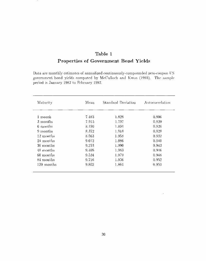
Table 1

Properties of Government Bond Yields

Data are monthly estimates of annualized continuously-compounded zero-coupon US

government boncl yielcls computed by MCCU11OC1Iand I{\von (1993). The sampleperiod is January 1982 to February 1992.

Maturity Mean Standard Deviation Autocorrelation

1 month

3 months6 months

9 months12 months24 months

36 months48 months

60 months84 months120 months

7.483

7.915

8.190

8.372

8.563

9.012

9.253

9.405

9.524

9.716

9.802

1.8281.7971.894

1.918

1.9581.9861.9901.98:3

1.9791.956

1.864

0.906

0.920

0.926

0.928

0.932

0.940

0.943

0.946

0.948

0,952

0.950

30

Figure 1. Mean Yields in Theory and Data10

7.5

7

x

x

x

M

x

Starsare data points, the line is theory

‘o 20 40 60 80 100 120

31

Figure 2. Two Choices of Ho–Lee Drift Parameters

,—. —-—,_. ——._. —-—.-. -.—’—.- .-”-

----,=. -

,,

/“/’ Match Expected Short Rates

//“

-3 -

\

Match Yield Curve

-4 -

-6- I 1 1 1 1 1 1 1

“o 5 10 15 20 25 30 35 40 45 50Time Horizon n in Months

32

120Figure 3. Ho and Lee Call Price Premium

80

60

40

20

5 10Time Tau to Expiration

(n=l)

15 20 25in Months

:3:3

Figure 4. Black-Derman–Toy Drift Parameters

00 5 10 15 20 25 30 35 40 45 50

Time Horizon n in Months

150

Figure 5. Black–Derman–Toy Call Price PremiumI 1 I 1

/

o1 1 1

0 5 10 15 20 25Bond Maturity n in Months

(tau=6)

:35

5

4

3

2

1

0

Figure 6. Black–Derman-Toy Exotic Price Premium1 I I 1 1 1 1 1 1

II 1 I I 1 I 1 I 1 1

-10 -8 -6 -4 -2 0 2 4 6 8 10Sensitivity Parameter Theta

(n=60)

Figure 7. Initial and Revised Volatility Parameters

Revised Volatility Curve

Initial Volatility Curve

2 4 6 8 10 12Date in Months

350

300

0

Figure 8. Average Risk–Adjusted Excess Returns

Benchmark

o 5 10 15 20Bond Maturity n in Months

(tau=2)

38

Ic

[.5

7

Figure 9. Theoretical Mean Yield Curve with Phi = 0.99

Stars are data points, the line is theory

o 20 40 60 80 100 120

:39