arbitrage profit. ross - university at albany · financial economics arbitrage pricing theory...
TRANSCRIPT
Financial Economics Arbitrage Pricing Theory
Arbitrage Pricing Theory
Ross ([1],[2]) presents the arbitrage pricing theory. The idea is
that the structure of asset returns leads naturally to a model of
risk premia, for otherwise there would exist an opportunity for
arbitrage profit.
1
Financial Economics Arbitrage Pricing Theory
Factor Model
Assume that there exists a risk-free asset, and consider a factor
model for the excess return ξ on a set of assets:
ξ = m+B�f + e.
The mean excess return m is the vector of risk premia.
2
Financial Economics Arbitrage Pricing Theory
Here
E(f) = 0
Var(f) = I,
and
E(e) = 0
Var(e) = D.
Here D is diagonal, and f and e are uncorrelated. One refers
to f as factors. The beta coefficients B are also called factor
loadings.
3
Financial Economics Arbitrage Pricing Theory
Systematic Versus Non-Systematic Risk
Assume that most of the components of B are not near zero.
The diagonal elements of D are not too large, and the number
of assets n is large.
Then the term B�f represents most of the variation in the
returns. Interpret B�f as the systematic risk, and e as the
non-systematic risk. One can argue that the non-systematic risk
can be eliminated by diversification, so the beta coefficients B
should determine the risk premium.
4
Financial Economics Arbitrage Pricing Theory
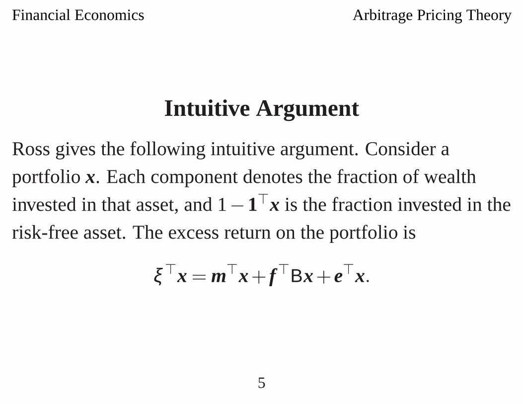
Intuitive Argument
Ross gives the following intuitive argument. Consider a
portfolio x. Each component denotes the fraction of wealth
invested in that asset, and 1−1�x is the fraction invested in the
risk-free asset. The excess return on the portfolio is
ξ �x = m�x+ f�Bx+ e�x.
5
Financial Economics Arbitrage Pricing Theory
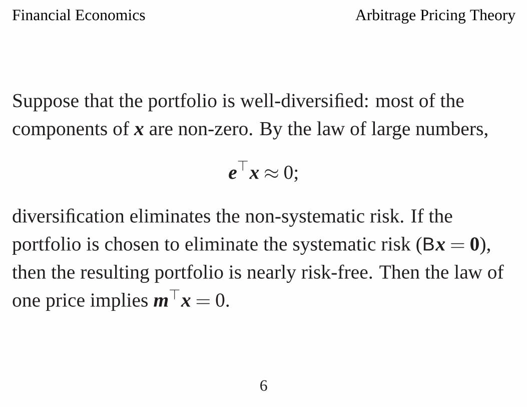
Suppose that the portfolio is well-diversified: most of the
components of x are non-zero. By the law of large numbers,
e�x ≈ 0;
diversification eliminates the non-systematic risk. If the
portfolio is chosen to eliminate the systematic risk (Bx = 0),
then the resulting portfolio is nearly risk-free. Then the law of
one price implies m�x = 0.
6
Financial Economics Arbitrage Pricing Theory
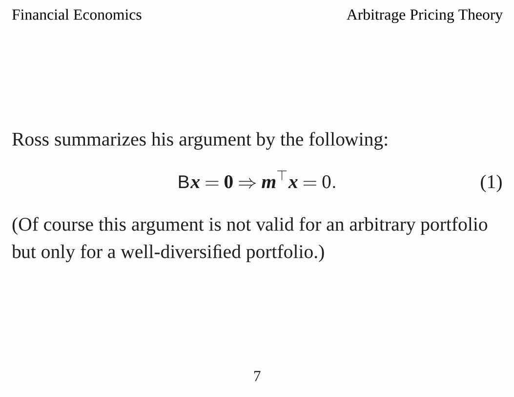
Ross summarizes his argument by the following:
Bx = 0 ⇒ m�x = 0. (1)
(Of course this argument is not valid for an arbitrary portfolio
but only for a well-diversified portfolio.)
7
Financial Economics Arbitrage Pricing Theory
Exact Factor Model
Consider first an exact factor model, in which e = 0 (so D = 0).
Remark 1 In the exact factor model, the law of one price is
equivalent to the condition (1).
8
Financial Economics Arbitrage Pricing Theory
Law of One Price
For the exact factor model, the law of one price (1) says that mis orthogonal to N(B). By the fundamental theorem of linear
algebra, m must lie in R(B�)
. Thus we obtain the following
theorem.
9
Financial Economics Arbitrage Pricing Theory
Theorem 2 (Arbitrage Pricing Theory) In the exact factor
model, the law of one price holds if only if the mean excess
return is a linear combination of the beta coefficients,
m = B�b, (2)
for some b.
10
Financial Economics Arbitrage Pricing Theory
The Arbitrage Pricing TheoryVersus the Capital-Asset Pricing Model
Like the capital-asset pricing model, the systematic risk
embodied in the beta coefficients determines the risk premia.
However the reasoning is different.
The capital-asset pricing model is derived from market
equilibrium, the equality of asset demand and supply. This
equality implies that the market portfolio must be efficient, and
a typical investor holds the market portfolio.
11
Financial Economics Arbitrage Pricing Theory
In contrast, the arbitrage pricing theory is derived from an
arbitrage argument, not a market equilibrium argument. The
risk premia (2) follow from the factor structure of the asset
returns. Asset supply is irrelevant to the argument. If some set
of asset returns has the factor structure, then the conclusion
follows for this set.
12

Financial Economics Arbitrage Pricing Theory
We next suppose that the factor model is not exact, that e �= 0.
Then any value for m is consistent with the law of one price
(the only portfolio with a constant excess return is x = 0).
Nevertheless we put forward a duality argument that (2) is a
good approximation.
13
Financial Economics Arbitrage Pricing Theory
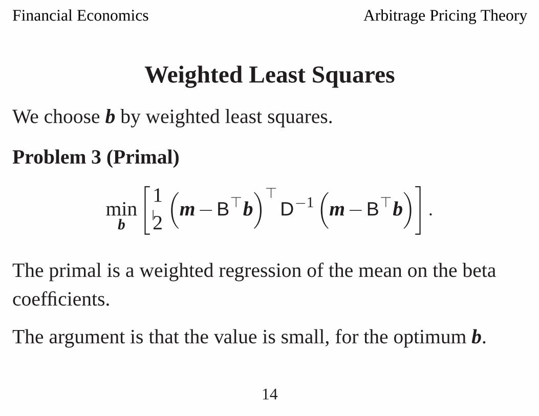
Weighted Least Squares
We choose b by weighted least squares.
Problem 3 (Primal)
minb
[12
(m−B�b
)�D−1
(m−B�b
)].
The primal is a weighted regression of the mean on the beta
coefficients.
The argument is that the value is small, for the optimum b.
14
Financial Economics Arbitrage Pricing Theory
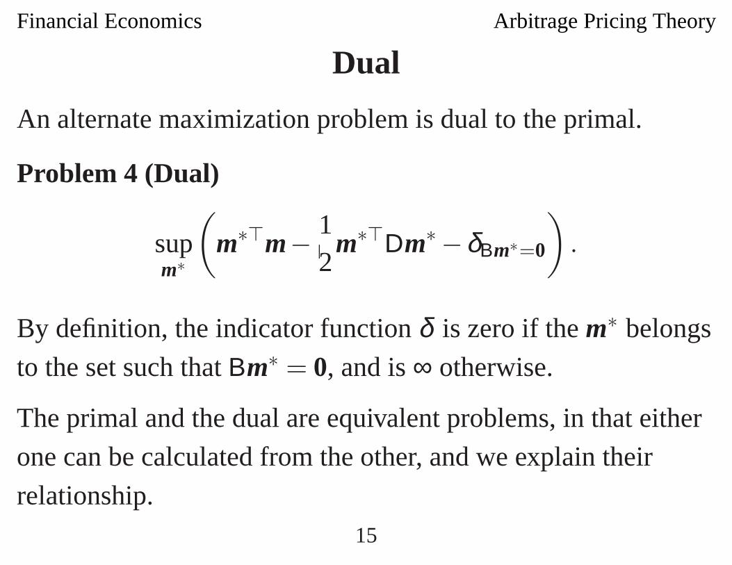
Dual
An alternate maximization problem is dual to the primal.
Problem 4 (Dual)
supm∗
(m∗�m− 1
2m∗�Dm∗ −δBm∗=0
).
By definition, the indicator function δ is zero if the m∗ belongs
to the set such that Bm∗ = 0, and is ∞ otherwise.
The primal and the dual are equivalent problems, in that either
one can be calculated from the other, and we explain their
relationship.15
Financial Economics Arbitrage Pricing Theory
The objective function of the primal is jointly convex in band m, and it follows that the value function V (m) is convex.
The choice variable is b, and the perturbation variable is m.
16
Financial Economics Arbitrage Pricing Theory
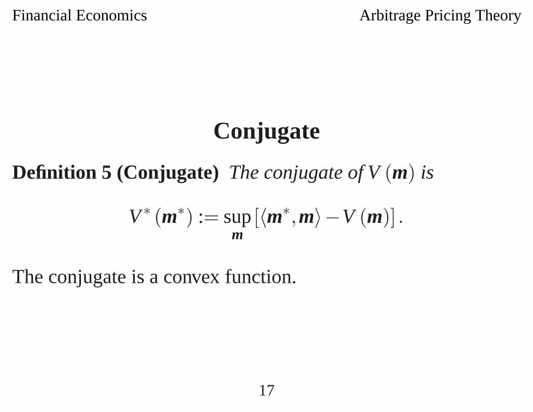
Conjugate
Definition 5 (Conjugate) The conjugate of V (m) is
V ∗ (m∗) := supm
[〈m∗,m〉−V (m)] .
The conjugate is a convex function.
17
Financial Economics Arbitrage Pricing Theory
Conjugate Duality
Proposition 6 (Conjugate Duality) Under general
conditions, the conjugate of the conjugate is the original
function,
V ∗∗ (m) = V (m) .
In mathematics, conjugate has many definitions, but always the
conjugate of the conjugate is the original; an example is the
complex conjugate.
18
Financial Economics Arbitrage Pricing Theory
Dual
Definition 7 (Dual) For a primal with value function V (m),the dual is the maximization problem
supm∗
[〈m∗,m〉−V ∗ (m∗)] .
By conjugate duality, the optimum value in the dual is V (m).
Theorem 8 (No Duality Gap) The minimum value in the
primal is the maximum value in the dual.
19
Financial Economics Arbitrage Pricing Theory
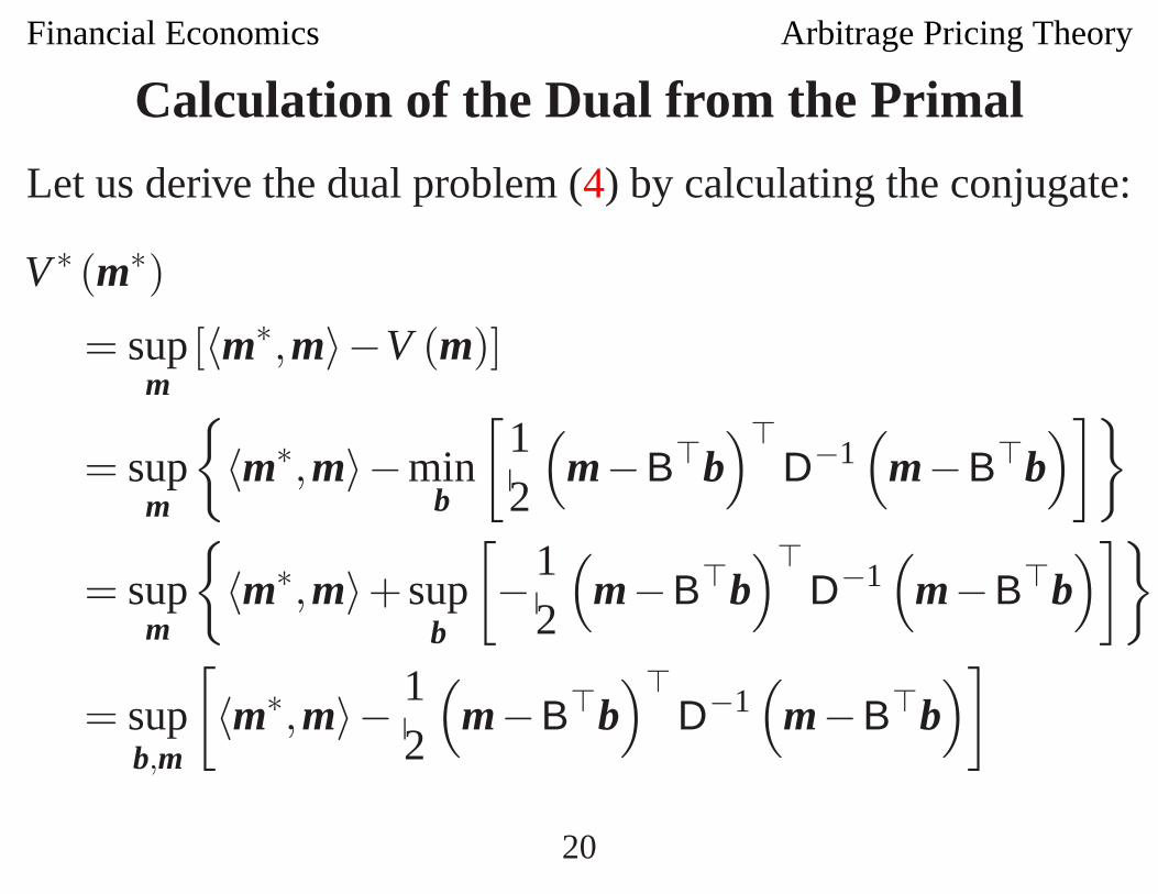
Calculation of the Dual from the Primal
Let us derive the dual problem (4) by calculating the conjugate:
V ∗ (m∗)
= supm
[〈m∗,m〉−V (m)]
= supm
{〈m∗,m〉−min
b
[12
(m−B�b
)�D−1
(m−B�b
)]}
= supm
{〈m∗,m〉+ sup
b
[−1
2
(m−B�b
)�D−1
(m−B�b
)]}
= supb,m
[〈m∗,m〉− 1
2
(m−B�b
)�D−1
(m−B�b
)]
20
Financial Economics Arbitrage Pricing Theory
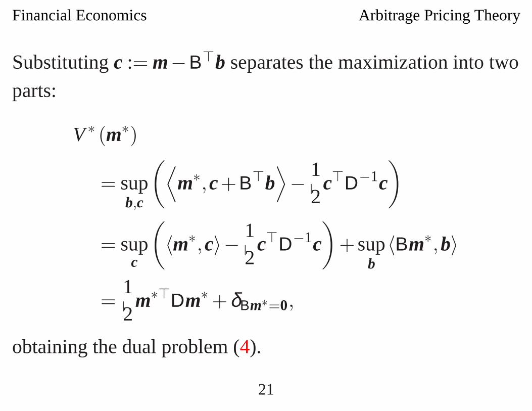
Substituting c := m−B�b separates the maximization into two
parts:
V ∗ (m∗)
= supb,c
(⟨m∗,c+B�b
⟩− 1
2c�D−1c
)
= supc
(〈m∗,c〉− 1
2c�D−1c
)+ sup
b〈Bm∗,b〉
=12
m∗�Dm∗ +δBm∗=0,
obtaining the dual problem (4).
21
Financial Economics Arbitrage Pricing Theory
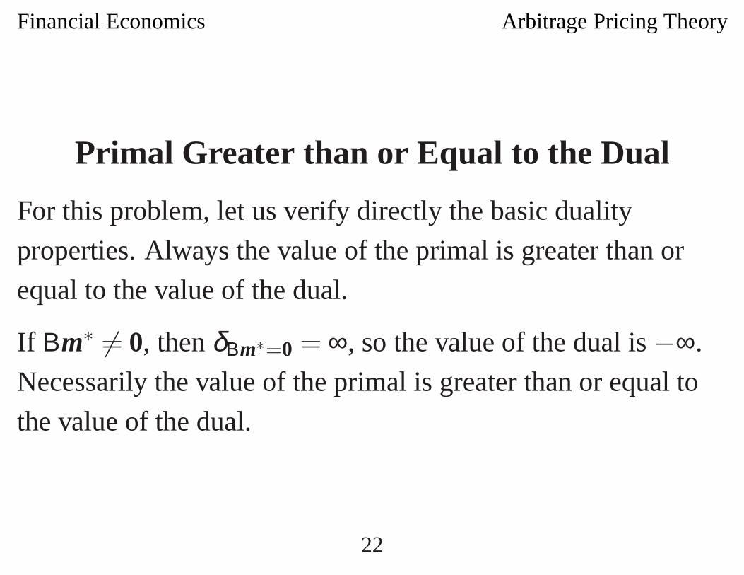
Primal Greater than or Equal to the Dual
For this problem, let us verify directly the basic duality
properties. Always the value of the primal is greater than or
equal to the value of the dual.
If Bm∗ �= 0, then δBm∗=0 = ∞, so the value of the dual is −∞.
Necessarily the value of the primal is greater than or equal to
the value of the dual.
22
Financial Economics Arbitrage Pricing Theory
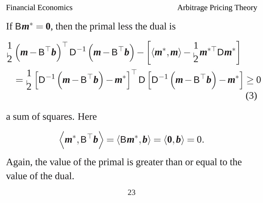
If Bm∗ = 0, then the primal less the dual is
12
(m−B�b
)�D−1
(m−B�b
)−
[〈m∗,m〉− 1
2m∗�Dm∗
]
=12
[D−1
(m−B�b
)−m∗
]�D
[D−1
(m−B�b
)−m∗
]≥ 0
(3)
a sum of squares. Here⟨m∗,B�b
⟩= 〈Bm∗,b〉 = 〈0,b〉 = 0.
Again, the value of the primal is greater than or equal to the
value of the dual.
23
Financial Economics Arbitrage Pricing Theory
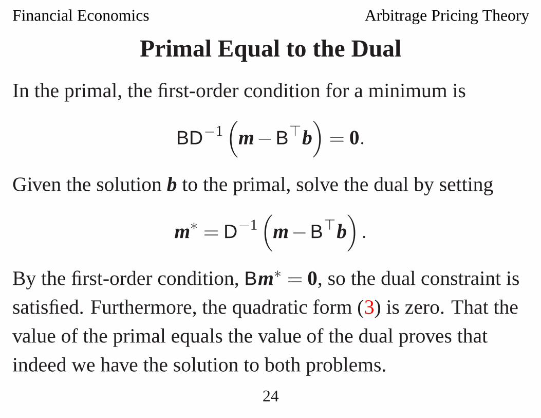
Primal Equal to the Dual
In the primal, the first-order condition for a minimum is
BD−1(
m−B�b)
= 0.
Given the solution b to the primal, solve the dual by setting
m∗ = D−1(
m−B�b)
.
By the first-order condition, Bm∗ = 0, so the dual constraint is
satisfied. Furthermore, the quadratic form (3) is zero. That the
value of the primal equals the value of the dual proves that
indeed we have the solution to both problems.
24
Financial Economics Arbitrage Pricing Theory
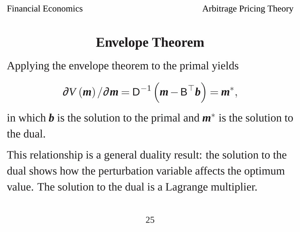
Envelope Theorem
Applying the envelope theorem to the primal yields
∂V (m)/∂m = D−1(
m−B�b)
= m∗,
in which b is the solution to the primal and m∗ is the solution to
the dual.
This relationship is a general duality result: the solution to the
dual shows how the perturbation variable affects the optimum
value. The solution to the dual is a Lagrange multiplier.
25
Financial Economics Arbitrage Pricing Theory
First-Order Condition Obsolete
Even though this verification makes use of the first-order
condition, a theme of duality theory is that the first-order
condition is obsolete. Because there is no duality gap, one can
solve the primal and the dual simultaneously, by setting the
primal equal to the dual. A systematic procedure then finds the
optimum values for the choice variables in the primal and the
dual, to achieve this equality.
26
Financial Economics Arbitrage Pricing Theory
Economic Interpretation of the Dual
The dual has an economic interpretation. The choice
variable m∗ is a portfolio of investments in the risky assets,
with 1−m∗�1 as the investment in the risk-free asset.
The constraint Bm∗ = 0 says that the portfolio is chosen to be
uncorrelated with the factors; the variability of the return arises
solely from the non-systematic risk.
Thus m∗�m is the excess return on the portfolio, and m∗�Dm∗
is the variance of the return.
27
Financial Economics Arbitrage Pricing Theory
The dual resembles the derivation of the separation theorem
with small risks, in which the objective function is a linear
function of the mean excess return and the variance.
Just as for the separation theorem, the solution to the dual
maximizes the ratio of the mean excess return to the standard
deviation,m∗�m√m∗�Dm∗ , (4)
here subject to the constraint that the portfolio return is
uncorrelated with the factors. Furthermore, the square of the
maximum value of this ratio is the optimum value of the dual.
28
Financial Economics Arbitrage Pricing Theory
Efficient Frontier
Define s̃ as the maximum value of the ratio (4). It is the slope
of an “efficient frontier,” subject to the constraint that the
portfolio return is uncorrelated with the factors.
The slope s of the efficient frontier is of course greater than or
equal to s̃.
29
Financial Economics Arbitrage Pricing Theory
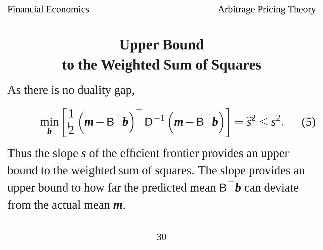
Upper Boundto the Weighted Sum of Squares
As there is no duality gap,
minb
[12
(m−B�b
)�D−1
(m−B�b
)]= s̃2 ≤ s2. (5)
Thus the slope s of the efficient frontier provides an upper
bound to the weighted sum of squares. The slope provides an
upper bound to how far the predicted mean B�b can deviate
from the actual mean m.
30
Financial Economics Arbitrage Pricing Theory
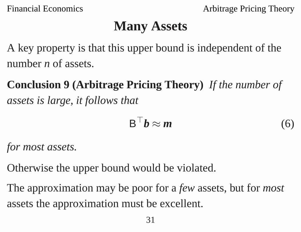
Many Assets
A key property is that this upper bound is independent of thenumber n of assets.
Conclusion 9 (Arbitrage Pricing Theory) If the number of
assets is large, it follows that
B�b ≈ m (6)
for most assets.
Otherwise the upper bound would be violated.
The approximation may be poor for a few assets, but for most
assets the approximation must be excellent.31
Financial Economics Arbitrage Pricing Theory
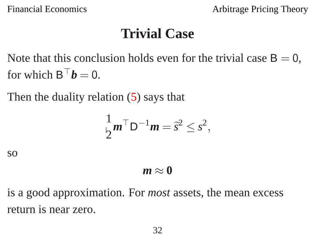
Trivial Case
Note that this conclusion holds even for the trivial case B = 0,
for which B�b = 0.
Then the duality relation (5) says that
12
m�D−1m = s̃2 ≤ s2,
so
m ≈ 0
is a good approximation. For most assets, the mean excess
return is near zero.
32
Financial Economics Arbitrage Pricing Theory
Irrelevance of Non-Systematic Risk?
Ross’s point of view is that the error e is non-systematic risk,
and this risk should be eliminated by portfolio diversification.
Hence the non-systematic risk should have no effect on mean
returns. If this point of view is true, then s̃ should be small,
small even if s is large.
By the duality relation (5), it would then follow that the
approximation (6) would be extremely good.
33
Financial Economics Arbitrage Pricing Theory
Diagonal Variance
That the variance of the error e is diagonal is important, and
allows one to see the error as non-systematic risk. The duality
relation (5) holds regardless of whether D is in fact diagonal.
If the components of e were highly correlated, then the
approximation (6) might be poor for many assets. For example,
for the trivial case B = 0, there is no presumption that most of
the components of m should be near zero.
34
Financial Economics Arbitrage Pricing Theory
References
[1] S. Ross. Return, risk, and arbitrage. In I. Friend and J. L.
Bicksler, editors, Risk and Return in Finance, pages
189–218. Ballinger, Cambridge, MA, 1977. HG4539R57.
[2] S. A. Ross. The arbitrage theory of capital asset pricing.
Journal of Economic Theory, 13(3):341–360, December
1976. HB1J645.
35