arch and garch models - wordpress.com overview of arima models arch model garch model garch-m model...
TRANSCRIPT
ARCH AND GARCH MODELS
Phung Thanh Binh
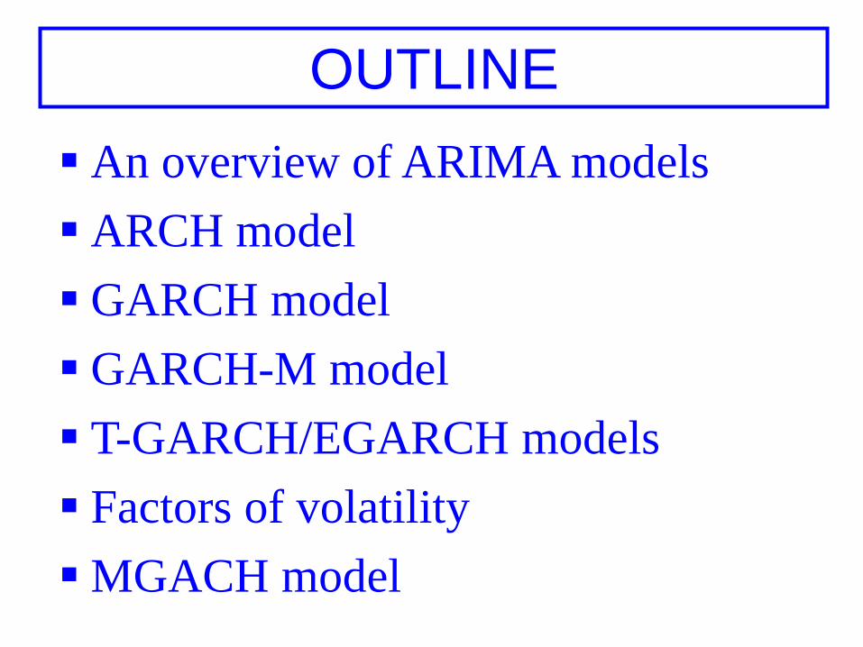
▪ An overview of ARIMA models
▪ ARCH model
▪ GARCH model
▪ GARCH-M model
▪ T-GARCH/EGARCH models
▪ Factors of volatility
▪ MGACH model
OUTLINE
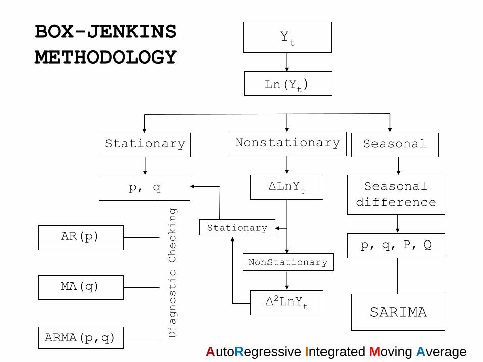
Ln(Yt)
Stationary Seasonal
Yt
Nonstationary
p, q
AR(p)
MA(q)
ARMA(p,q) Diagnostic Checking
∆LnYt
Stationary
NonStationary
∆2LnYt
Seasonal
difference
p, q, P, Q
SARIMA
BOX-JENKINS
METHODOLOGY
AutoRegressive Integrated Moving Average
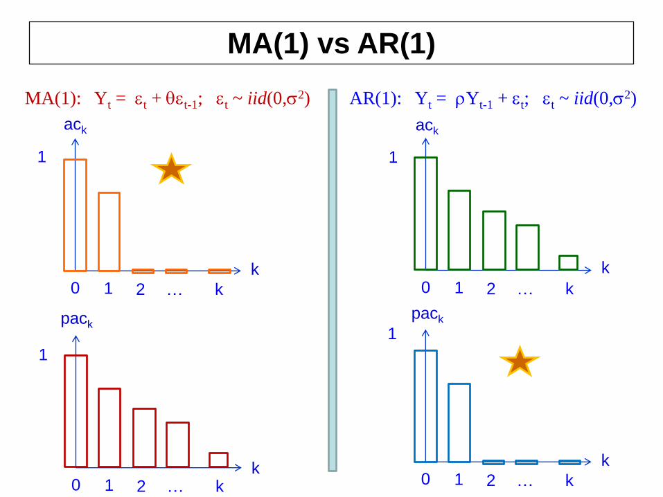
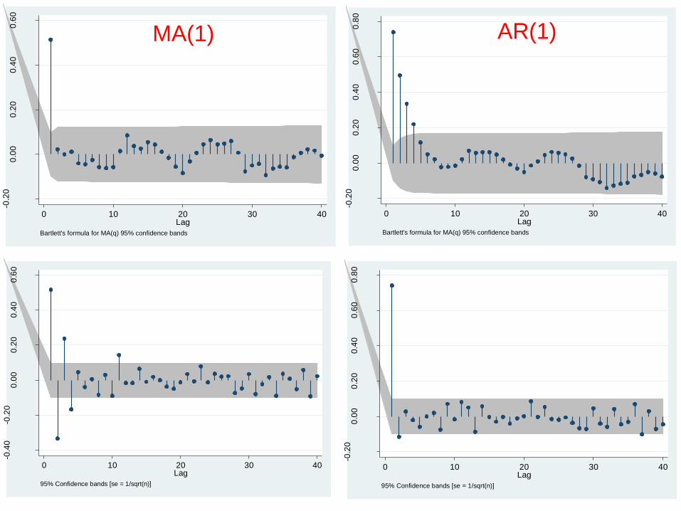
MA(1) vs AR(1)
MA(1): Yt = t + t-1; t ~ iid(0,2) AR(1): Yt = Yt-1 + t; t ~ iid(0,2)
ack
k0
1
1 2 k…
ack
k
0
1
1 2 k…
pack
k0
1
1 2 k…k
0
1
1 2 k…
pack
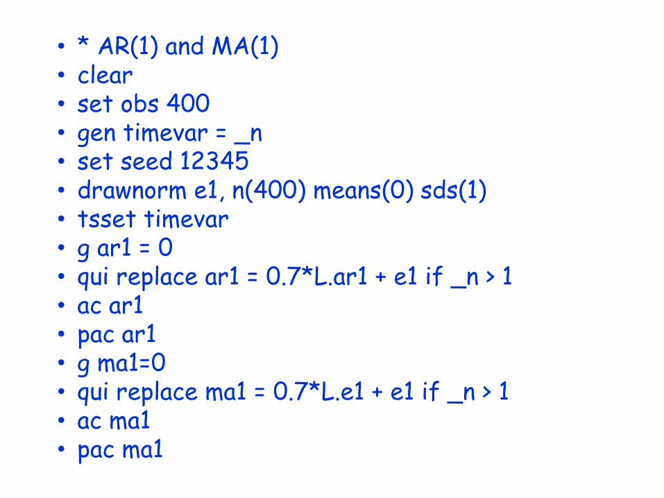
• * AR(1) and MA(1)• clear• set obs 400• gen timevar = _n• set seed 12345• drawnorm e1, n(400) means(0) sds(1)• tsset timevar• g ar1 = 0• qui replace ar1 = 0.7*L.ar1 + e1 if _n > 1• ac ar1• pac ar1• g ma1=0• qui replace ma1 = 0.7*L.e1 + e1 if _n > 1• ac ma1• pac ma1
-0.2
00
.00
0.2
00
.40
0.6
00
.80
Pa
rtia
l a
uto
co
rrela
tio
ns o
f a
r1
0 10 20 30 40Lag
95% Confidence bands [se = 1/sqrt(n)]
-0.2
00
.00
0.2
00
.40
0.6
00
.80
Au
tocorr
ela
tion
s o
f ar1
0 10 20 30 40Lag
Bartlett's formula for MA(q) 95% confidence bands
-0.2
00
.00
0.2
00
.40
0.6
0
Au
tocorr
ela
tion
s o
f m
a1
0 10 20 30 40Lag
Bartlett's formula for MA(q) 95% confidence bands
AR(1)MA(1)
-0.4
0-0
.20
0.0
00
.20
0.4
00
.60
Pa
rtia
l a
uto
co
rrela
tio
ns o
f m
a1
0 10 20 30 40Lag
95% Confidence bands [se = 1/sqrt(n)]
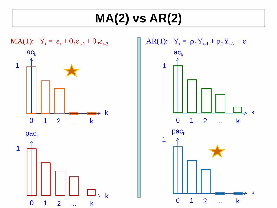
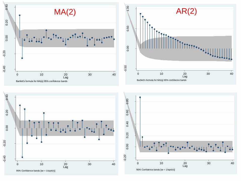
MA(2) vs AR(2)
MA(1): Yt = t + 1t-1 + 2t-2 AR(1): Yt = 1Yt-1 + 2Yt-2 + t
ack
k0
1
1 2 k…
ack
k
0
1
1 2 k…
pach
k0
1
1 2 k…k
0
1
1 2 k…
pack

• * AR(2) and MA(2)• clear• set obs 400• gen timevar = _n• set seed 12345• drawnorm e1, n(400) means(0) sds(1)• tsset timevar• g double ar2 = 0• qui replace ar2 in 3/l = 0.6*L.ar2 + 0.3*L2.ar2 + e1• ac ar2• pac ar2• g double ma2=0• qui replace ma2 in 3/l = 0.6*L.e1 - 0.4*L2.e1 + e1• ac ma2• pac ma2
-0.4
0-0
.20
0.0
00
.20
0.4
0
Au
tocorr
ela
tion
s o
f m
a2
0 10 20 30 40Lag
Bartlett's formula for MA(q) 95% confidence bands
-0.4
0-0
.20
0.0
00
.20
0.4
0
Pa
rtia
l a
uto
co
rrela
tio
ns o
f m
a2
0 10 20 30 40Lag
95% Confidence bands [se = 1/sqrt(n)]
-0.5
00
.00
0.5
01
.00
Au
tocorr
ela
tion
s o
f ar2
0 10 20 30 40Lag
Bartlett's formula for MA(q) 95% confidence bands
-0.2
00
.00
0.2
00
.40
0.6
00
.80
Pa
rtia
l a
uto
co
rrela
tio
ns o
f a
r2
0 10 20 30 40Lag
95% Confidence bands [se = 1/sqrt(n)]
AR(2)MA(2)
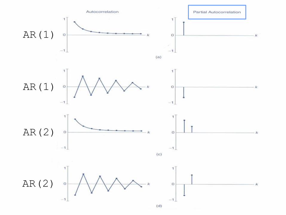
AR(1)
AR(1)
AR(2)
AR(2)
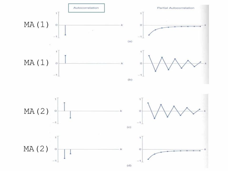
MA(1)
MA(2)
MA(2)
MA(1)
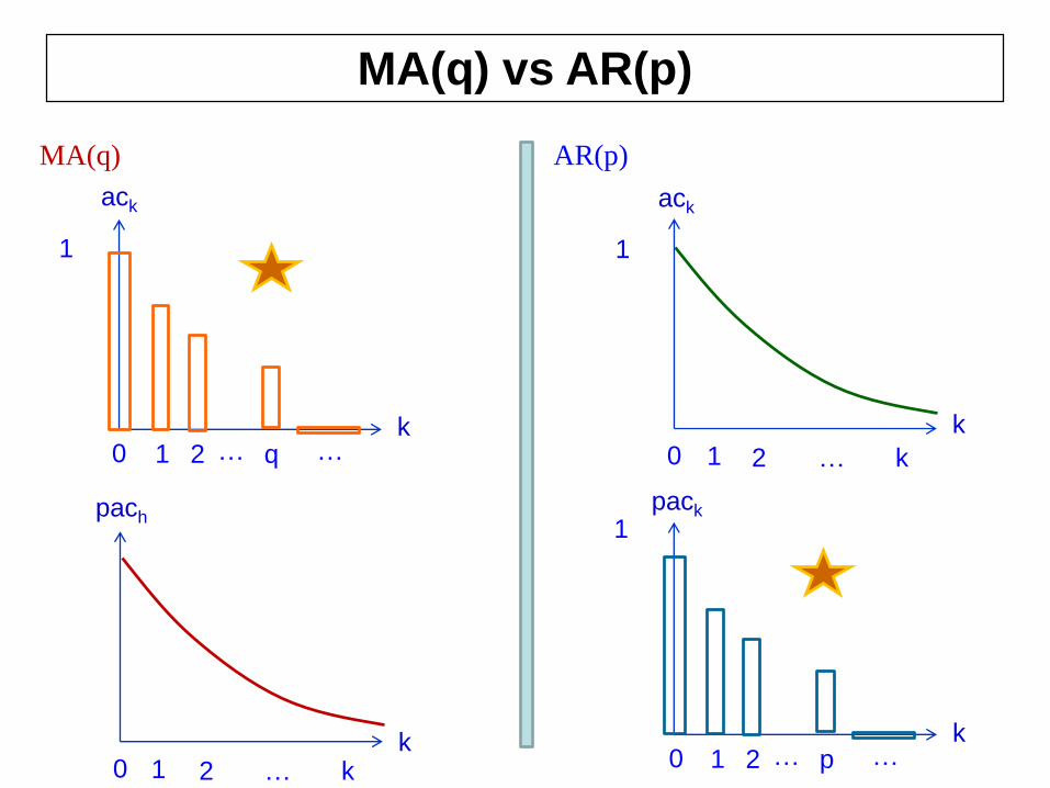
MA(q) vs AR(p)
MA(q) AR(p)
ack
k0
1
1 2 …
ack
k
0
1
1 2 k…
pack
k
1
k0 1 2 k…
pach
q …
0 1 2 … p …
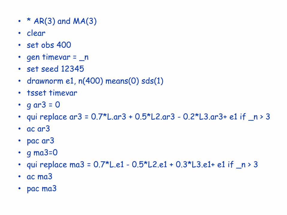
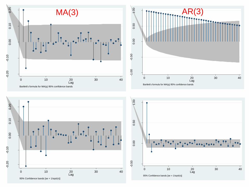
• * AR(3) and MA(3)
• clear
• set obs 400
• gen timevar = _n
• set seed 12345
• drawnorm e1, n(400) means(0) sds(1)
• tsset timevar
• g ar3 = 0
• qui replace ar3 = 0.7*L.ar3 + 0.5*L2.ar3 - 0.2*L3.ar3+ e1 if _n > 3
• ac ar3
• pac ar3
• g ma3=0
• qui replace ma3 = 0.7*L.e1 - 0.5*L2.e1 + 0.3*L3.e1+ e1 if _n > 3
• ac ma3
• pac ma3
-0.2
0-0
.10
0.0
00
.10
0.2
0
Au
tocorr
ela
tion
s o
f m
a3
0 10 20 30 40Lag
Bartlett's formula for MA(q) 95% confidence bands
-0.2
0-0
.10
0.0
00
.10
0.2
0
Pa
rtia
l a
uto
co
rrela
tio
ns o
f m
a3
0 10 20 30 40Lag
95% Confidence bands [se = 1/sqrt(n)]
-1.0
0-0
.50
0.0
00
.50
1.0
0
Au
tocorr
ela
tion
s o
f ar3
0 10 20 30 40Lag
Bartlett's formula for MA(q) 95% confidence bands
-0.5
00
.00
0.5
01
.00
Pa
rtia
l a
uto
co
rrela
tio
ns o
f a
r3
0 10 20 30 40Lag
95% Confidence bands [se = 1/sqrt(n)]
AR(3)MA(3)
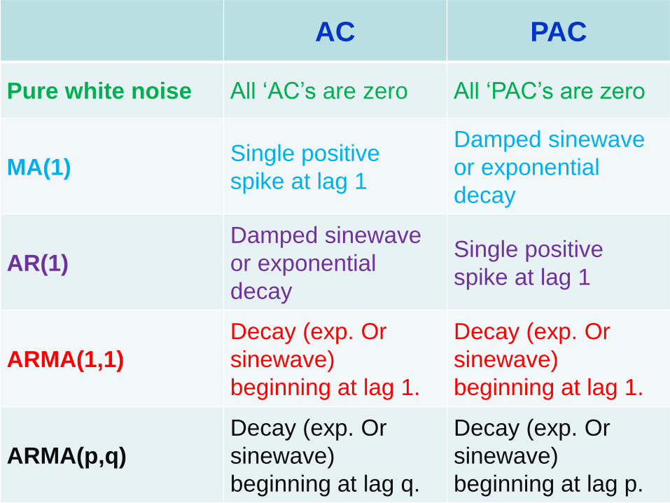
AC PAC
Pure white noise All ‘AC’s are zero All ‘PAC’s are zero
MA(1)Single positive
spike at lag 1
Damped sinewave
or exponential
decay
AR(1)
Damped sinewave
or exponential
decay
Single positive
spike at lag 1
ARMA(1,1)
Decay (exp. Or
sinewave)
beginning at lag 1.
Decay (exp. Or
sinewave)
beginning at lag 1.
ARMA(p,q)
Decay (exp. Or
sinewave)
beginning at lag q.
Decay (exp. Or
sinewave)
beginning at lag p.
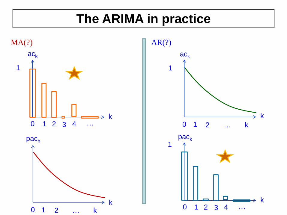
The ARIMA in practice
MA(?) AR(?)
ack
k0
1
1 2
ack
k
0
1
1 2 k…
pack
k
1
k0 1 2 k…
pach
4 …
0 1 2 4 …
3
3
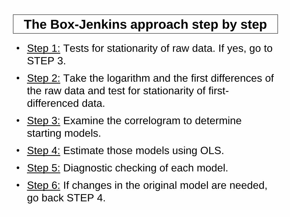
• Step 1: Tests for stationarity of raw data. If yes, go to
STEP 3.
• Step 2: Take the logarithm and the first differences of
the raw data and test for stationarity of first-
differenced data.
• Step 3: Examine the correlogram to determine
starting models.
• Step 4: Estimate those models using OLS.
• Step 5: Diagnostic checking of each model.
• Step 6: If changes in the original model are needed,
go back STEP 4.
The Box-Jenkins approach step by step
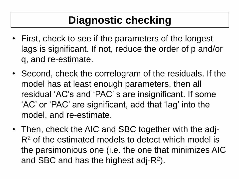
• First, check to see if the parameters of the longest
lags is significant. If not, reduce the order of p and/or
q, and re-estimate.
• Second, check the correlogram of the residuals. If the
model has at least enough parameters, then all
residual ‘AC’s and ‘PAC’ s are insignificant. If some
‘AC’ or ‘PAC’ are significant, add that ‘lag’ into the
model, and re-estimate.
• Then, check the AIC and SBC together with the adj-
R2 of the estimated models to detect which model is
the parsimonious one (i.e. the one that minimizes AIC
and SBC and has the highest adj-R2).
Diagnostic checking
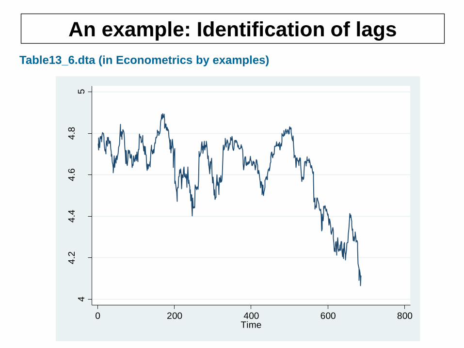
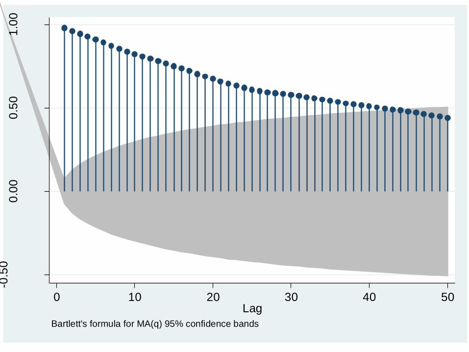
An example: Identification of lags
Table13_6.dta (in Econometrics by examples)
44
.24
.44
.64
.85
ln(c
lose
)
0 200 400 600 800Time
-0.5
00
.00
0.5
01
.00
Au
tocorr
ela
tion
s o
f ln
clo
se
0 10 20 30 40 50Lag
Bartlett's formula for MA(q) 95% confidence bands
-0.1
0-0
.05
0.0
00
.05
0.1
0
Au
tocorr
ela
tion
s o
f D
.ln
clo
se
0 10 20 30 40 50Lag
Bartlett's formula for MA(q) 95% confidence bands


-0.1
0-0
.05
0.0
00
.05
0.1
0
Au
tocorr
ela
tion
s o
f D
.ln
clo
se
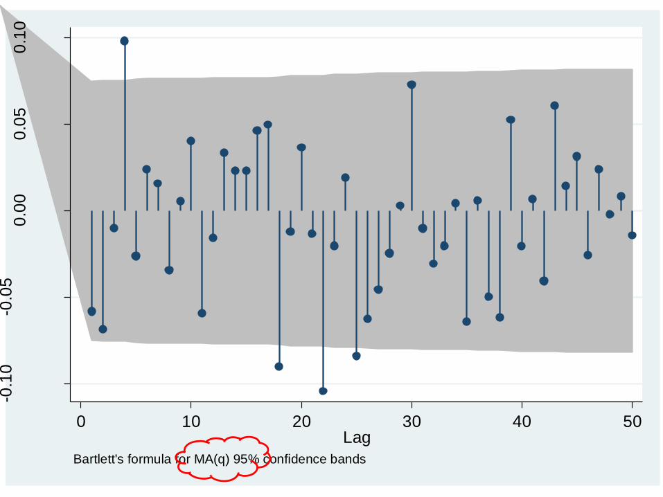
0 2 4 6 8 10 12 14 16 18 20 22 24 26 28 30 32 34 36 38 40 42 44 46 48 50Lag
Bartlett's formula for MA(q) 95% confidence bandsac d.lnclose, lags(50)
q = (4, 18, 22, 25)
-0.1
0-0
.05
0.0
00
.05
0.1
0
Pa
rtia
l a
uto
co
rrela
tio
ns o
f D
.lnclo
se
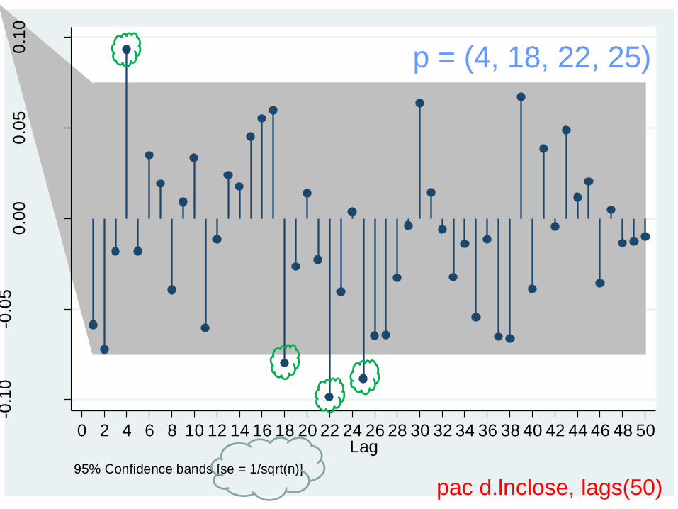
0 2 4 6 8 10 12 14 16 18 20 22 24 26 28 30 32 34 36 38 40 42 44 46 48 50Lag
95% Confidence bands [se = 1/sqrt(n)]
p = (4, 18, 22, 25)
pac d.lnclose, lags(50)
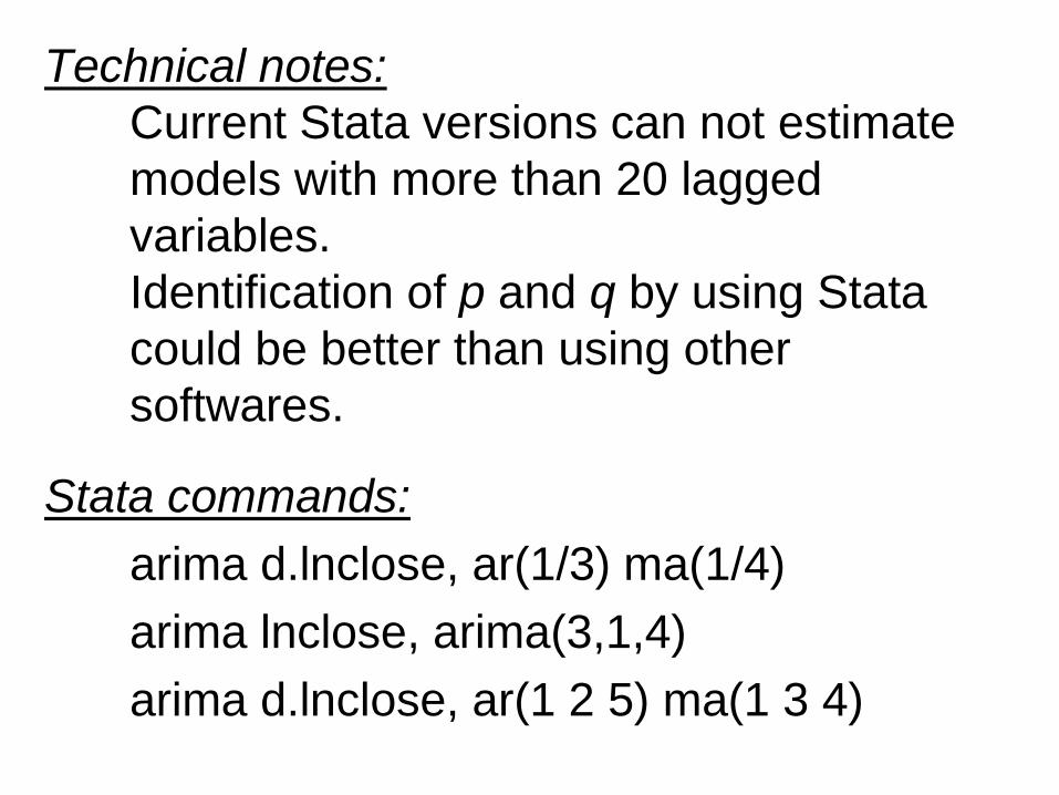
Technical notes:
Current Stata versions can not estimate
models with more than 20 lagged
variables.
Identification of p and q by using Stata
could be better than using other
softwares.
Stata commands:
arima d.lnclose, ar(1/3) ma(1/4)
arima lnclose, arima(3,1,4)
arima d.lnclose, ar(1 2 5) ma(1 3 4)
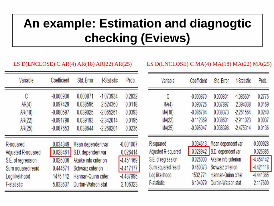
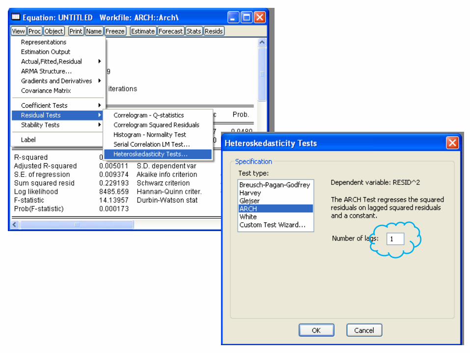
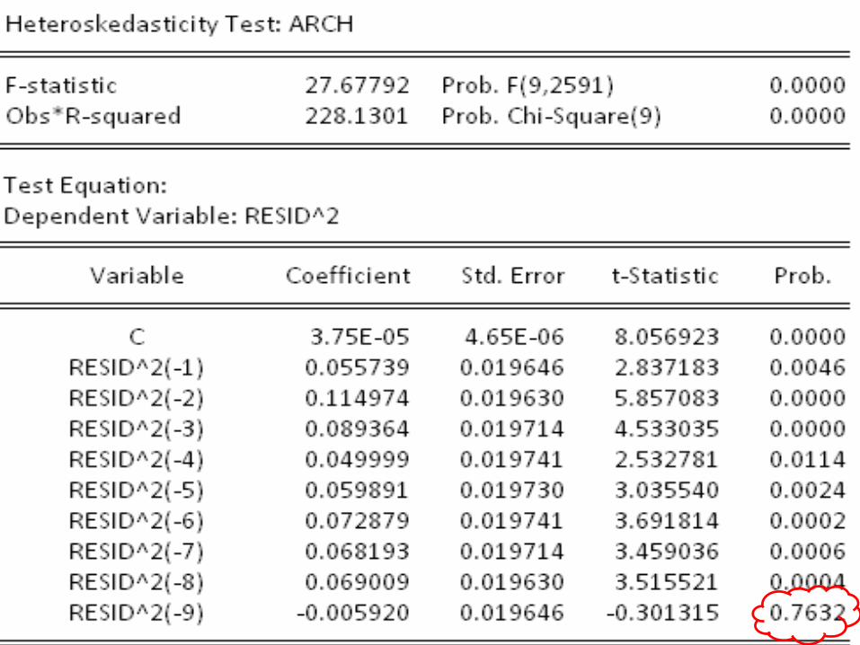
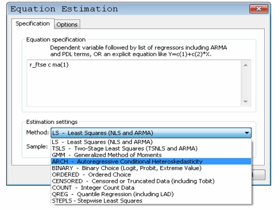
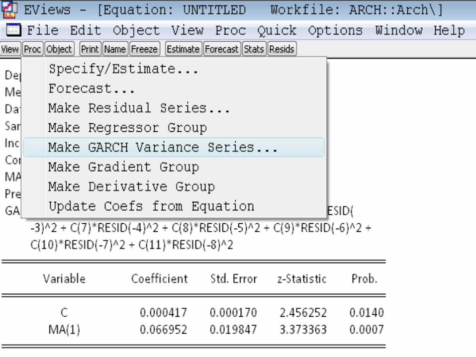
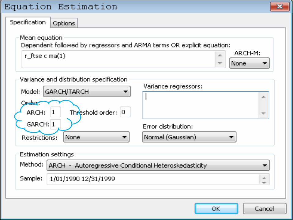
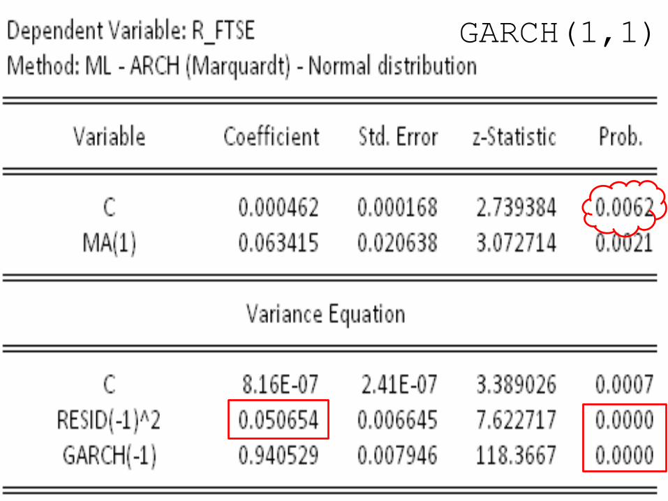
An example: Estimation and diagnogtic
checking (Eviews)
LS D(LNCLOSE) C AR(4) AR(18) AR(22) AR(25) LS D(LNCLOSE) C MA(4) MA(18) MA(22) MA(25)
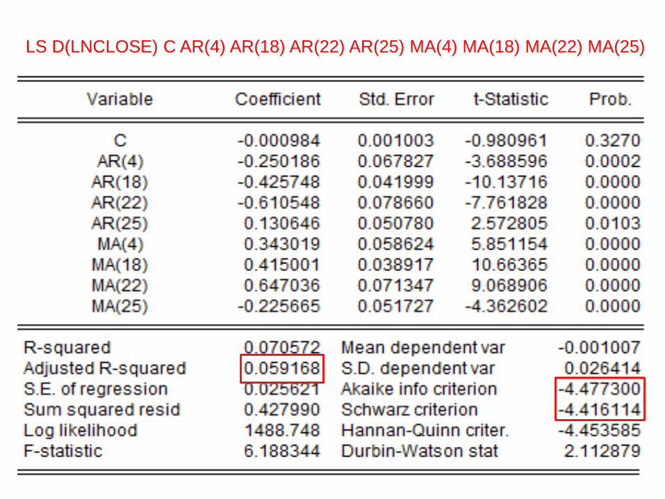
LS D(LNCLOSE) C AR(4) AR(18) AR(22) AR(25) MA(4) MA(18) MA(22) MA(25)

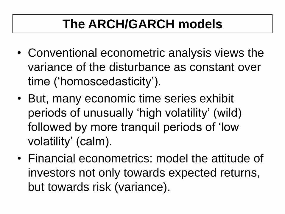
• Conventional econometric analysis views the
variance of the disturbance as constant over
time (‘homoscedasticity’).
• But, many economic time series exhibit
periods of unusually ‘high volatility’ (wild)
followed by more tranquil periods of ‘low
volatility’ (calm).
• Financial econometrics: model the attitude of
investors not only towards expected returns,
but towards risk (variance).
The ARCH/GARCH models
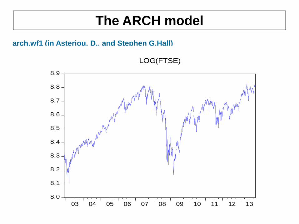
The ARCH model
arch.wf1 (in Asteriou, D., and Stephen G.Hall)
8.0
8.1
8.2
8.3
8.4
8.5
8.6
8.7
8.8
8.9
03 04 05 06 07 08 09 10 11 12 13
LOG(FTSE)
-.100
-.075
-.050
-.025
.000
.025
.050
.075
.100
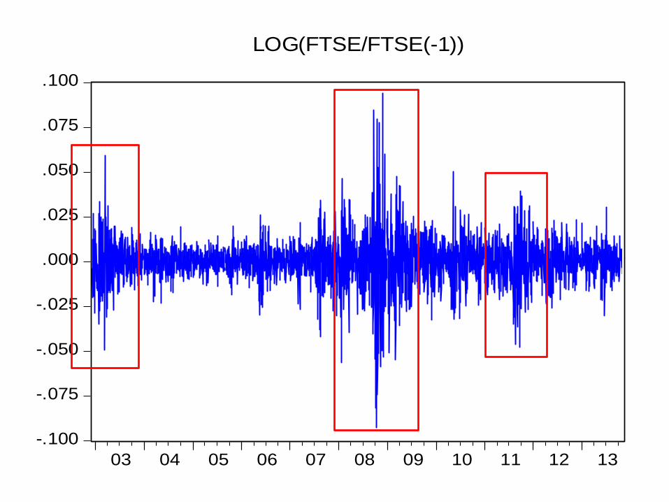
03 04 05 06 07 08 09 10 11 12 13
LOG(FTSE/FTSE(-1))
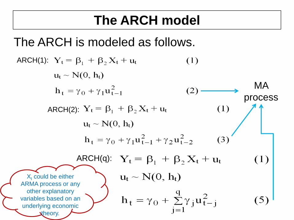
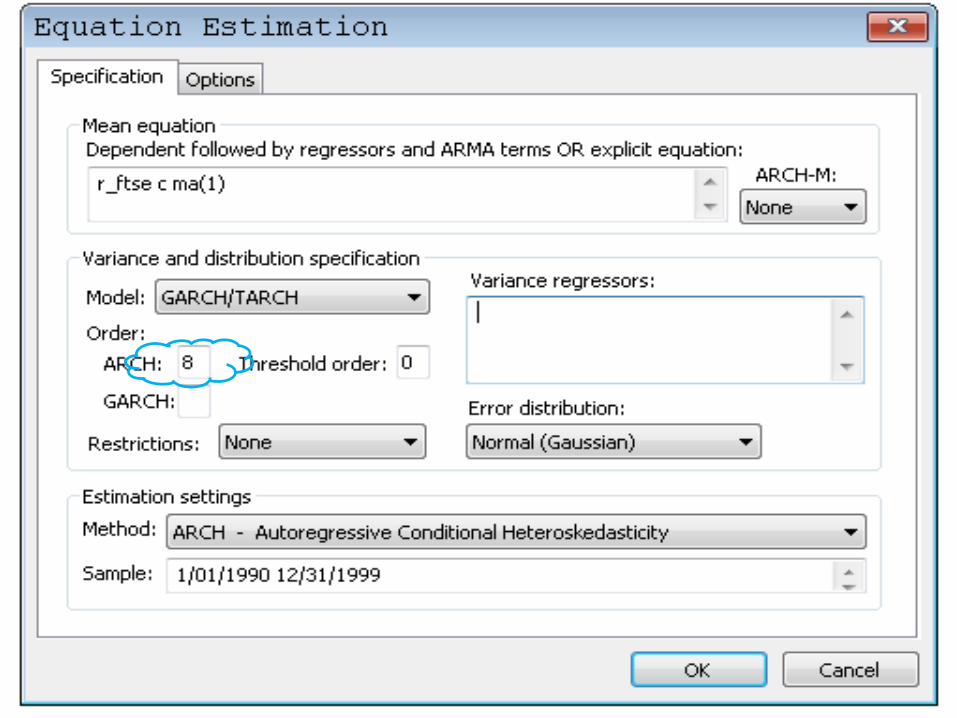
The ARCH model
The ARCH is modeled as follows.
ARCH(1):
ARCH(2):
ARCH(q):
MA
process
Xt could be either
ARMA process or any
other explanatory
variables based on an
underlying economic
theory.
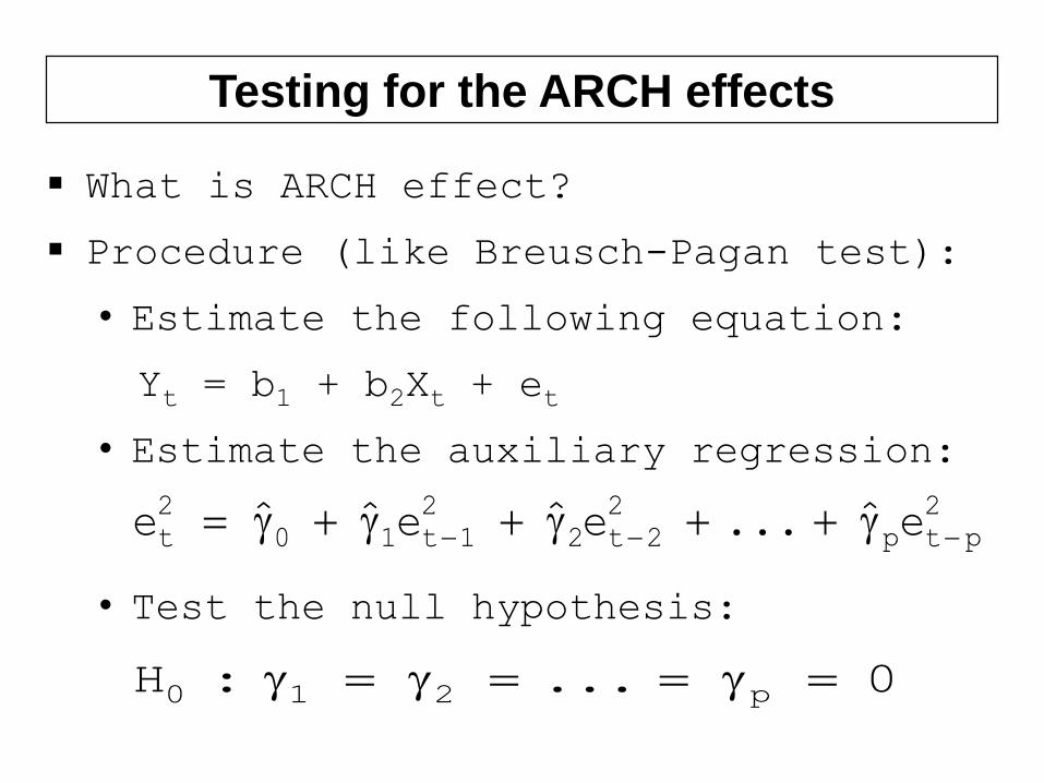
Testing for the ARCH effects
▪ What is ARCH effect?
▪ Procedure (like Breusch-Pagan test):
• Estimate the following equation:
Yt = b1 + b2Xt + et
• Estimate the auxiliary regression:
• Test the null hypothesis:
2
ptp
2
2t2
2
1t10
2
t eˆ...eˆeˆˆe
0...:H p210

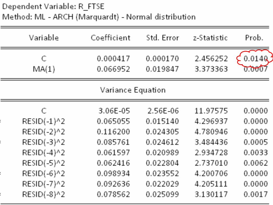
An example: FTSE volatility
▪ Suppose the series FTSE follows
ARIMA(0,1,1) model:
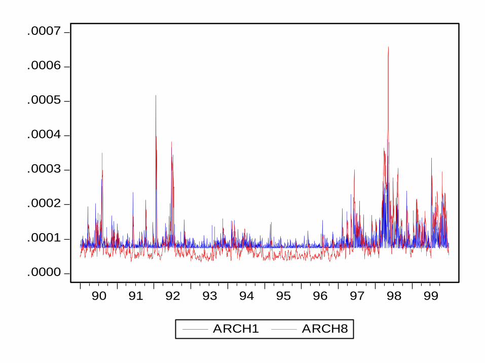
.0000
.0001
.0002
.0003
.0004
.0005
.0006
.0007
90 91 92 93 94 95 96 97 98 99
ARCH1 ARCH8
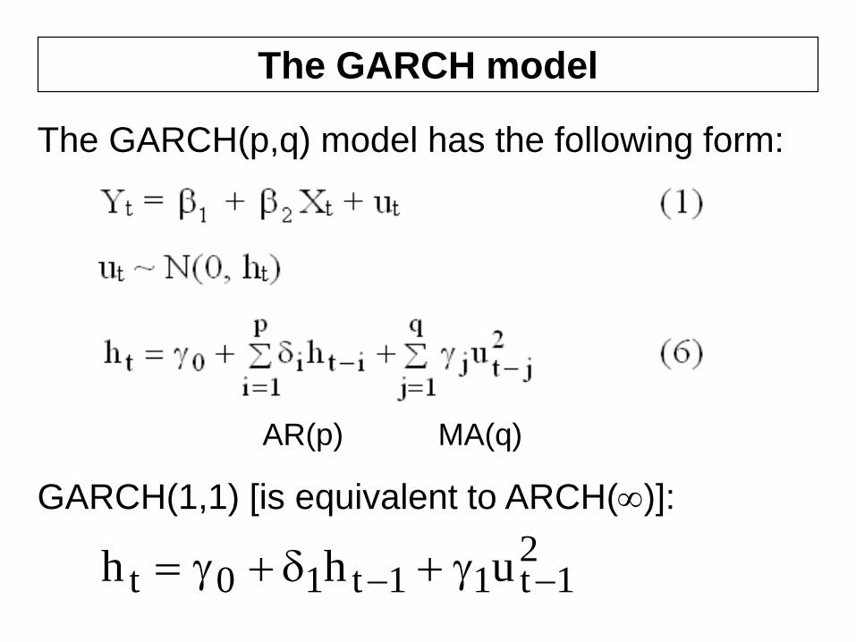
The GARCH model
The GARCH(p,q) model has the following form:
GARCH(1,1) [is equivalent to ARCH()]:
21t11t10t uh h
AR(p) MA(q)
▪ The coefficient (1 + 1)
measures the volatility shock.
If it is very close to unity,
volatility shocks are
persistent, which means that the
conditional variance converges
to the steady state quite
slowly. This indicates that it
may take a relatively long time
to return to a steady state.
The GARCH model
GARCH(1,1)
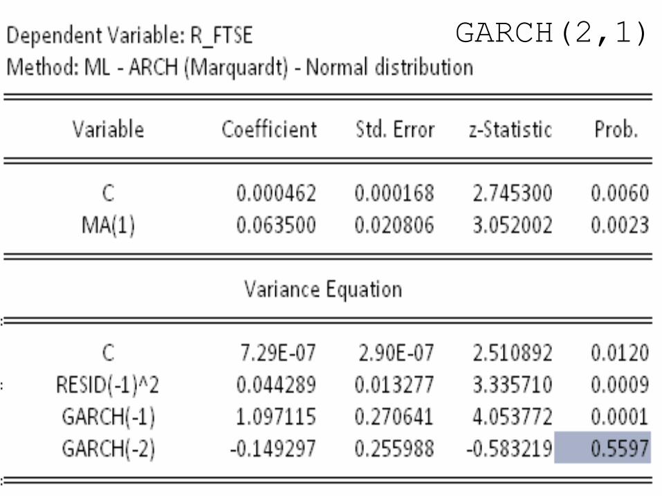
GARCH(2,1)
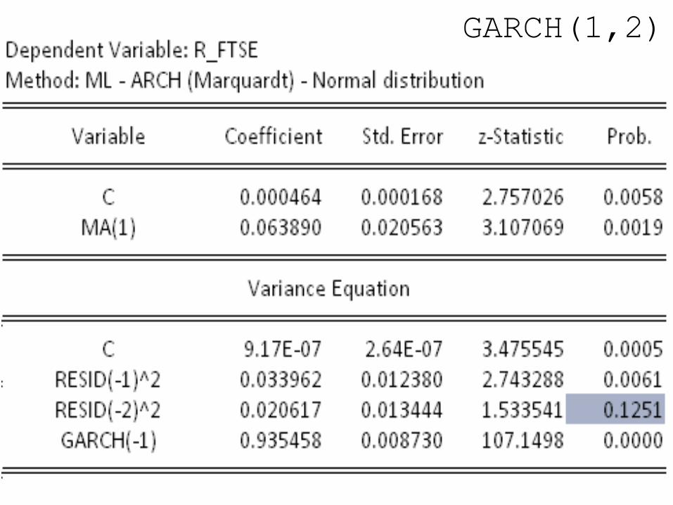
GARCH(1,2)

GARCH(3,2)
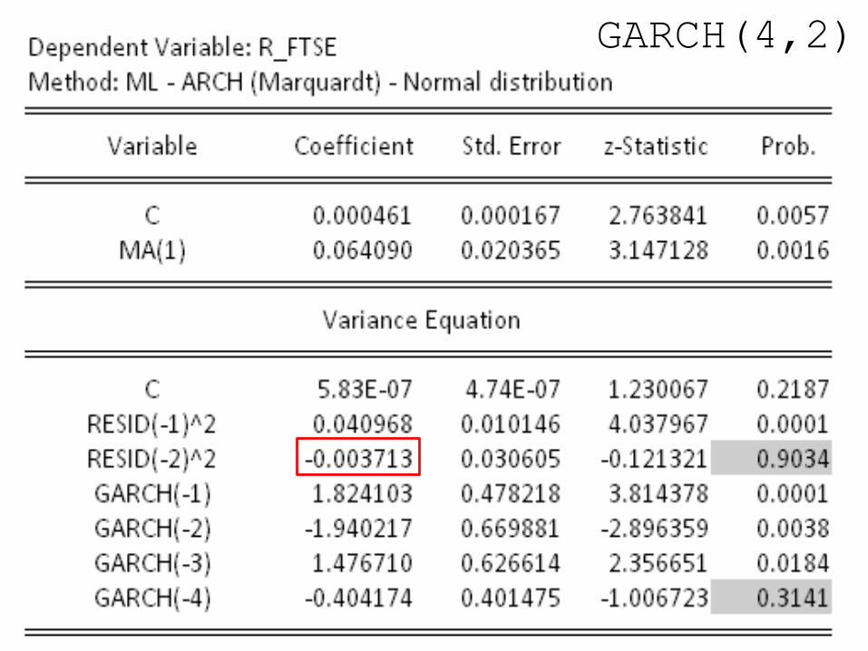
GARCH(4,2)
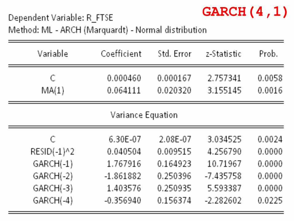
GARCH(4,1)
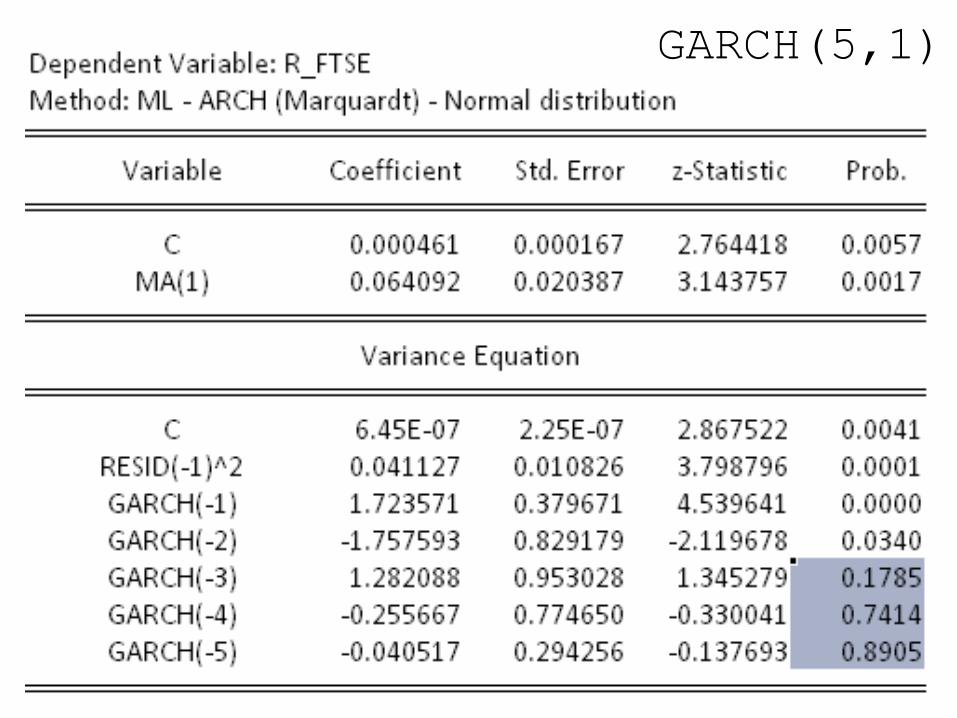
GARCH(5,1)
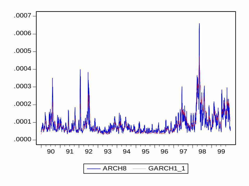
.0000
.0001
.0002
.0003
.0004
.0005
.0006
.0007
90 91 92 93 94 95 96 97 98 99
ARCH8 GARCH1_1
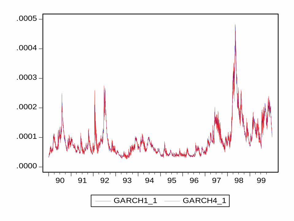
.0000
.0001
.0002
.0003
.0004
.0005
90 91 92 93 94 95 96 97 98 99
GARCH1_1 GARCH4_1
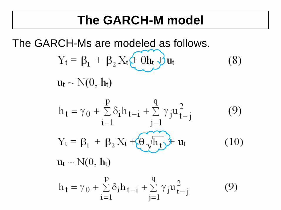
The GARCH-M model
The GARCH-Ms are modeled as follows.
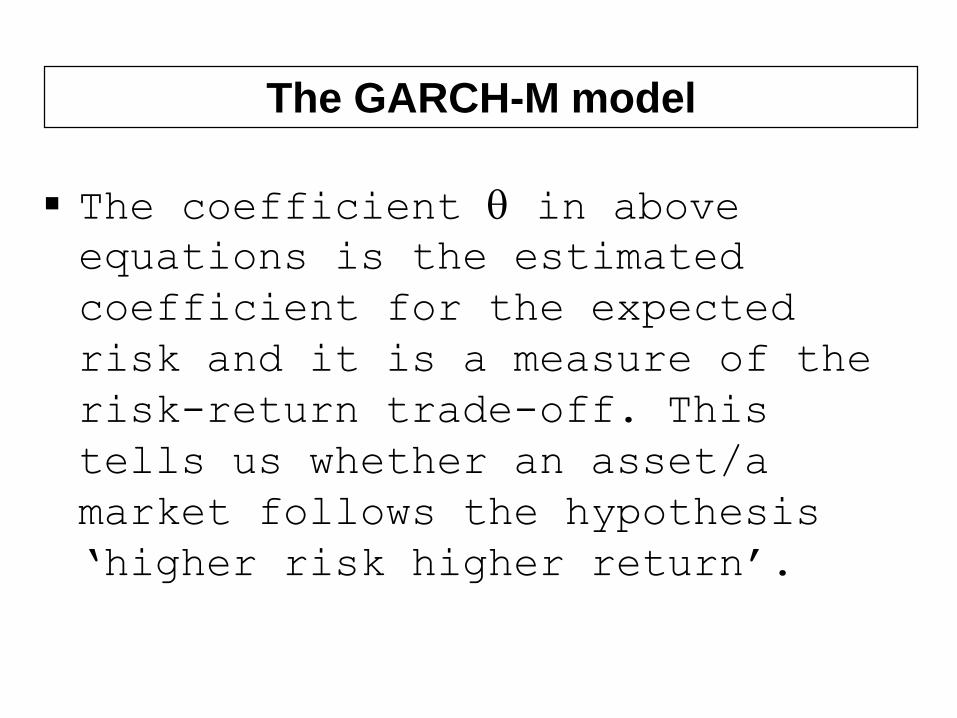
▪ The coefficient in above
equations is the estimated
coefficient for the expected
risk and it is a measure of the
risk-return trade-off. This
tells us whether an asset/a
market follows the hypothesis
‘higher risk higher return’.
The GARCH-M model
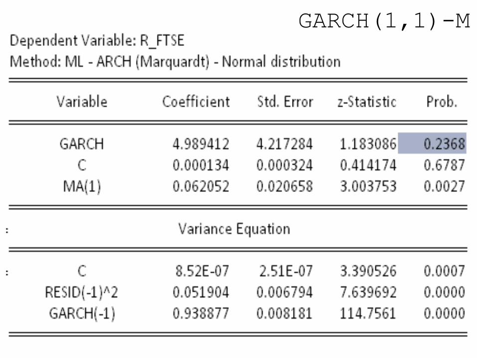
GARCH(1,1)-M
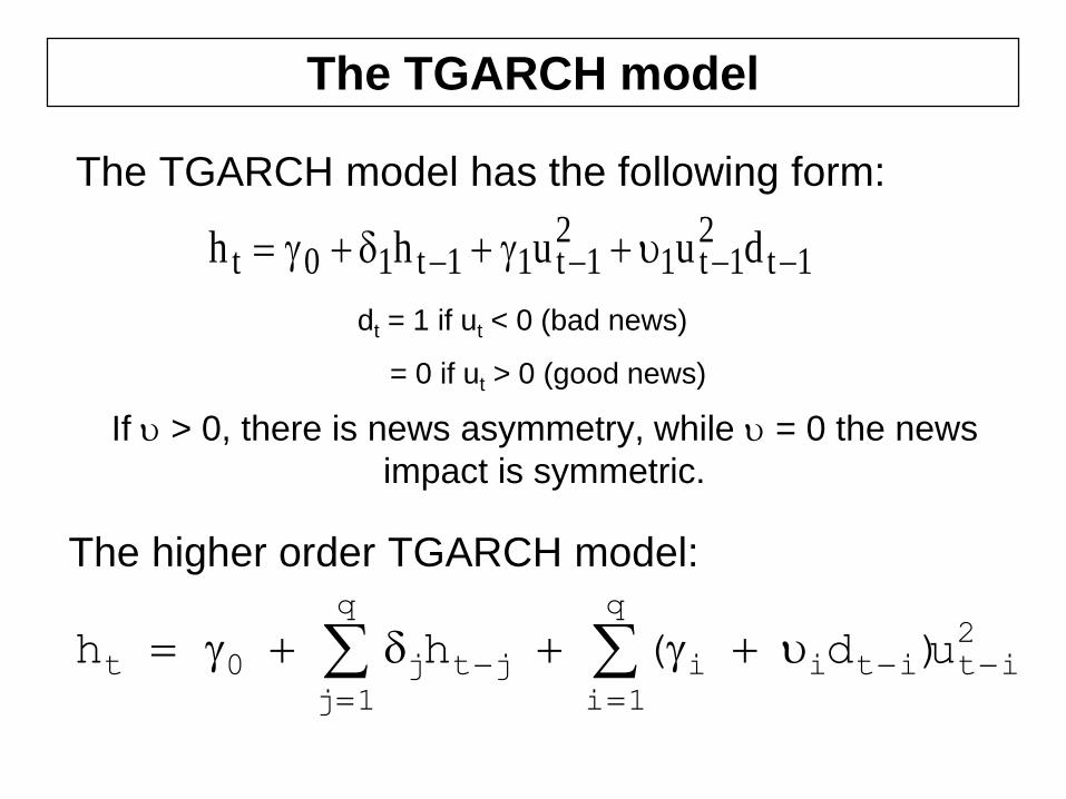
The TGARCH model
1t2
1t12
1t11t10t duuh h
The TGARCH model has the following form:
If > 0, there is news asymmetry, while = 0 the news
impact is symmetric.
The higher order TGARCH model:
2
it
q
1i
itiijt
q
1j
j0t u)d(h h
dt = 1 if ut < 0 (bad news)
= 0 if ut > 0 (good news)
The EGARCH model
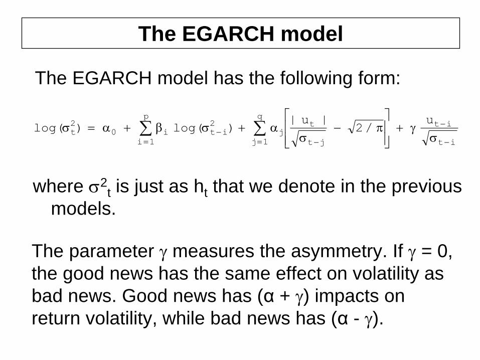
The EGARCH model has the following form:
it
it
jt
tq
1j
j
2
it
p
1i
i0
2
t
u/2
|u|)log()log(
where 2t is just as ht that we denote in the previous
models.
The parameter measures the asymmetry. If = 0,
the good news has the same effect on volatility as
bad news. Good news has (α + ) impacts on
return volatility, while bad news has (α - ).
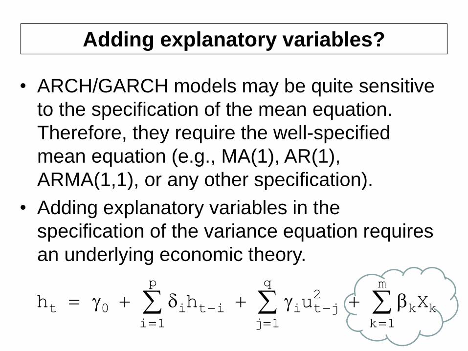
• ARCH/GARCH models may be quite sensitive
to the specification of the mean equation.
Therefore, they require the well-specified
mean equation (e.g., MA(1), AR(1),
ARMA(1,1), or any other specification).
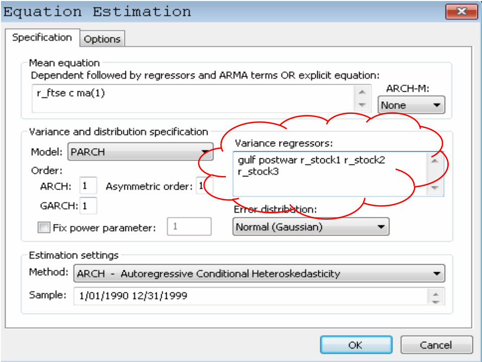
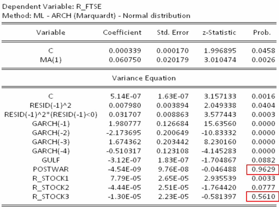
• Adding explanatory variables in the
specification of the variance equation requires
an underlying economic theory.
Adding explanatory variables?
k
m
1k
k
2
jt
q
1j
iit
p
1i
i0t Xuh h

• The above models are univariate ARCH-type models. For
doing research, it’s better to use multivariate GARCH
(MGARCH) models. These models have various
applications:
• Volatility of a market leads to volatility of other markets.
• Volatility of an asset leads to volatility of other assets.
• Shock on a market increases the volatility on another
market.
• Impact of volatility in financial markets on real economic
variables.
• The computation of time-varying hedge ratios.
• The estimation of time-varying beta coefficient in asset
pricing models, etc.
Multivariate GARCH model