ARCHETYPAL ANALYSIS

By

Adele CutlerMathematics and Statistics

Utah State UniversityLogan, UT 84322-3900

Leo BreimanDepartment of StatisticsUniversity of CaliforniaBerkeley, CA 94720

Technical Report No. 379revised October 1993

Department of StatisticsUniversity of CaliforniaBerkeley, CA 94720

ARCHETYPAL ANALYSIS

Adele Cutler Leo Breiman

Mathematics and Statistics Department of Statistics

Utah State University University of California

Logan, UT 84322-3900 Berkeley, CA 94720

Abstract

Archetypal analysis represents each "individual" in a data set as a mixture of "in-

dividuals of pure type", or "archetypes". The archetypes themselves are restricted to

be mixtures of the individuals in the data set. Archetypes are selected by minimizing

the squared error in representing each individual as a mixture of archetypes. The use-

fulness of archetypal analysis is illustrated on a number of data sets. Computing the

archetypes is a nonlinear least squares problem which is solved using an alternating

minimizing algorithm.

KEY WORDS: Archetypes, principal components, convex hull, graphics, nonlin-

ear optimization.

1

1. INTRODUCTION

For multivariate data {z,i,i = 1,...,n} where each z, is an m-vector zi

(Xi ... i xmi)t an interesting problem is to find m-vectors z,...., zp that characterize

the "archetypal patterns" in the data. For instance, a data set analyzed by Flury and

Riedwyl (1988) consists of 6 head dimensions for 200 Swiss soldiers. The purpose of

the data was to help design face masks for the Swiss Army.

A natural question is whether there are a few "pure types" or "archetypes" of

heads such that the 200 heads in the data base are mixtures of the archetypal heads.

One possible answer is provided by a variant of principal components. For given

m-vectors zl,... ,zp, the linear combination Xk aikzk that best approximates zi is

defined as the minimizer of

iz, C-ZaikZkll.k

Then the "best patterns" zl,.. . , zp are the minimizers of

Z l|i-EZ ikzk ||l * (1.1)i k

Without loss of generality, take z1,.. . ,zzp to be orthonormal. Then the minimizers

of (1.1) maximizep

E 4SZk (1.2)

where S = X'X. The maximizers of (1.2) are the eigenvectors of S corresponding

to the p largest eigenvalues. Thus, if each zt is centered at its mean, the solution is

given by the principal components decomposition.

2

The "patterns" derived this way are usually not an answer to the problem posed

above. For instance, the first four "patterns" found using the Swiss Army data do not

correspond to any real or even fictitious heads. In some of the patterns, the distance

between two points on the head is negative.

This is not surprising, given that the principal components approach nowhere

requires either that the "patterns" resemble "pure types" in the data, or that each

xi be approximated by a mixture of the patterns (i.e. Caik > 0, Ek aik = 1).

In archetypal analysis the patterns zl, . . . , zp considered are mixtures of the data

values {ai}. Furthermore, the only approximations to x allowed are mixtures of the

{Zk}.

More precisely, for fixed zj,... , zp where

ZkZEpkjZj, k= 1,...p

and fki . 0, Pki = 1, define the {rik}, k = 1,.. .,p as the minimizers of

p

i-E CikZkI|k=1

under the constraints ask . 0, k, aik = 1. Then define the archetypal patterns or

archetypes as the mixtures zl, ... , zp that minimize

p

E IIi - crikZklIi k=1

and denote the minimum value by RSS(p). For p > 1, the archetypes fall on the

convex hull of the data (see Section 3). Thus the archetypes are extreme data-values

3

such that all of the data can be well-represented as convex mixtures of the archetypes.

But the archetypes themselves are not wholly mythological, since each is constrained

to be a mixture of points in the data.

In contrast to principal components analysis, archetype analysis does not nest,

nor are the successive archetypes orthogonal to one another. As more archetypes are

found, the existing ones can change to better capture the shape of the dataset. How-

ever, as we hope the examples will show, archetypes can give a uniquely informative

way to understand multivariate data and curves.

The paper is organized as follows: Section 2 gives examples of archetype analysis

as applied to data. Section 3 discusses the locations of the archetypes. Section

4 contains a description at the algorithm used to compute archetypes. Section 5

contains some results regarding convergence of the algorithm and Section 6 gives a

brief summary.

Previous work that has the flavor of archetypal analysis is mainly based on princi-

pal components. A natural approach is to use the quantiles of the principal component

scores to select "representative" individuals. For example Jones and Rice (1992) use

principal components to summarize a large number of curves. The principal compo-

nents themselves are informative, but additional information is obtained by selecting

the curves corresponding to the median, minimum, and maximum values of the prin-

cipal component score. However, such choices may be misleading, particularly if the

4

principal components themselves are difficult to interpret.

Flury and Tarpey (1992) suggest that if extreme curves are required, they might

be chosen by considering those curves for which the Mahalanobis distance from the

mean is large. However, the curves with large Mahalanobis distance may in fact be

very similar to each other, and may not reflect the extremes present in the data.

The analysis of the Swiss Army data (Example 2.1) by Flury (1993) was based

on "principal points", a concept similar to that of cluster centers. This method

has also been used to get representative curves as an alternative to the Jones-Rice

approach (see Flury 1990, 1993). One feature of principal points which is not shared

by archetypes is that principal points is a concept for theoretical distributions.

Other related work is that of Woodbury and Clive (1974), who use maximum

likelihood estimation based on grades of membership to derive "pure types". Similar

ideas are also evident in latent class analysis (Lazarsfeld and Henry, 1968) and latent

budget analysis (De Leeuw and van der Heijden 1991, van der Heijden et al. 1992).

2. EXAMPLES

The three following examples illustrate how archetypes can be used to understand

data structure. The first example, involving head measurements of Swiss Army sol-

diers, is given because of its intuitive appeal. The second and third examples are

more serious applications, involving air pollution and Tokamak fusion data.

5

2.1. Swiss Army Head Dimension Data

The Swiss Army data consists of six measurements on each head. Two are mea-

sures of the width of the face just above the eyes and just below the mouth. The

3rd is the distance from the top of the nose to the chin, the 4th the length of nose,

and the 5th and 6th are the distances from the ear to the top of the nose and chin

respectively. Figure 1 pictures the archetypal heads for p = 2,3,4,5.

These pictures (Figure 1) are given as graphical illustration of the idea of archetypes.

They are "extreme" or 'pure" types as patterns such that each real individual can

be well approximated by a mixture of the "pure types" or archetypes.

Figure 2 shows the values of 100 x RSS(p)/RSS(1). In Section 3, we note that

for p = 1, the single archetype is the mean of the {zi}. Thus RSS(1) is simply the

total sum-of-squares Fi lIzi -: 112 and the ratio 100 x RSS(p)/RSS(l) measures the

percent decrease in squared error when p archetypes are used to represent the data.

2.2. Air Pollution Data

This data consists of measurements of data relevant to air pollution in the Los

Angeles Basin in 1976. There are 330 complete cases consisting of daily measurements

on the variables

* ozone (OZONE)

* 500 millibar height (500MH)

6

* wind speed (WDSP)

* humidity (HMDTY)

* surface temperature (STMP)

* inversion base height (INVHT)

* pressure gradient (PRGRT)

* inversion base temperature (INVTMP)

* visibility (VZBLTY)

These data were standardized to have mean zero and variance one, and archetypes

were computed. Figure 3 is a graph of 100 x RSS(p)/RSS(l). We focus on three

archetypes.

Figure 4 displays the percentile value of each variable in an archetype as compared

to the data. For example, the height of the first bar for OZONE in Archetype 1 is

92. This indicates that the OZONE value in archetype 1 is in the 92nd percentile of

the 330 OZONE readings in the data.

Archetype 1 is high in OZONE, 500MH, HMDTY, STMP, INVTMP and low

in INVHT and VZBLTY. This indicates a typical hot summer day. The nature of

the other two archetypes is less clear. The PRGRT is predominantly measured in

the north-south direction. A low percentile value indicates a large negative pressure

7

gradient, and a high value, a large positive gradient. The differences in PRGRT and

WDSP in archetypes 2 and 3 indicates a connection with air mass motion in the

basin. The temperatures are lower in archetype 3, so it seems to represent cooler

days towaxd winter.

We can get more insight by looking at another graphical representation. With

three archetypes zl, Z2, Z3, the vector of variables zi for the ith day is best ap-

proximated by the mixture zx l a,ilz + ai2Z2 + ai3Z3. There is a simple way to

get a two-dimensional data representation. Let 1s,, 2213 be the vertices of a two-

dimensional equilateral triangle, and map z, -H pi, i = 1,2, 3. Then. we represent xi

by ct,ill + ai2J2 + ai3p3-

Figure 5 a) - d) gives such plots separately for each of the four seasons. Clearly,

the summer days cluster close to the 1st archetype. Spring mixes mainly the 1st and

3rd; Fall, the 1st and 2nd; and Winter the 2nd and 3rd.

The archetype mixture coefficients can also be used to see how the individual

variables vary as functions of archetypes. For instance, let the mixture coefficients

of the ith day's data be ail, ai2, ai3. If Oi is the OZONE value for the ith day, we

would generally expect O0 to be large if a,l is close to one, and smaller otherwise (see

Figure 4).

To make this more specific, O, was regressed on terms of up to 3rd degree in ail,

a,2, a,i3 (actually only on terms in ali, ai2 since ail + ai2 + a,3 = 1). The resulting

8

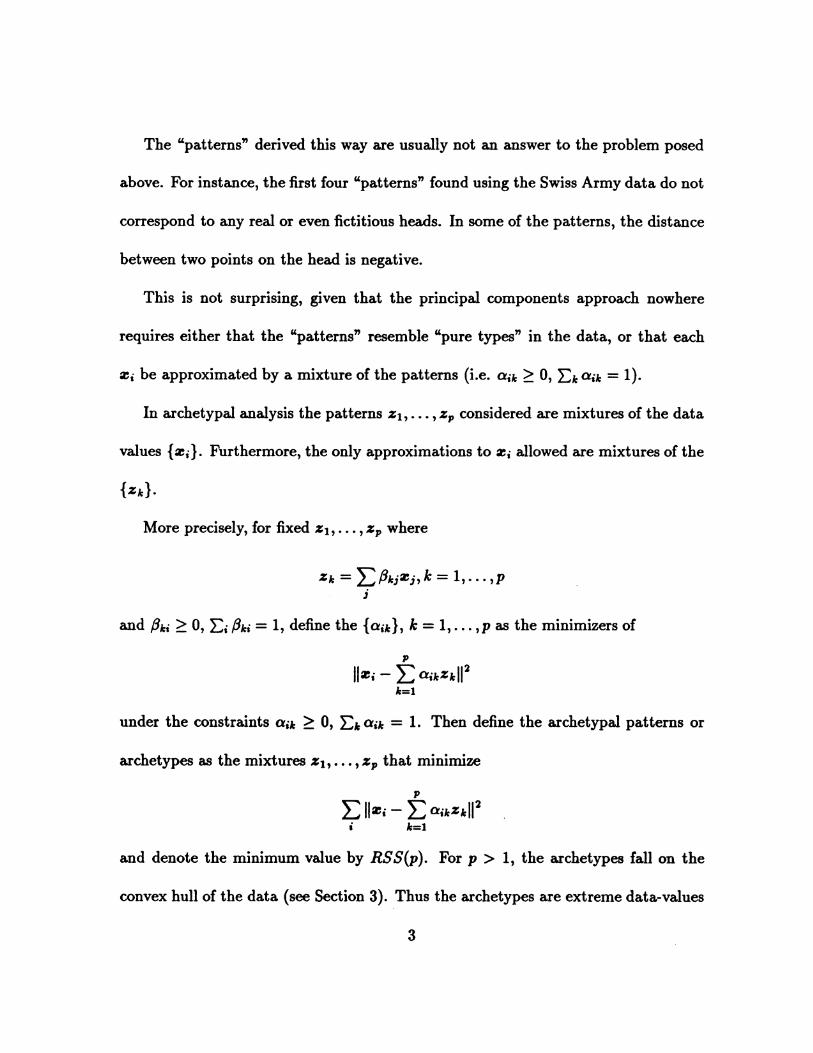
prediction equation for OZONE as a function of cal, a!2, aC3 is plotted as a surface in

Figure 6(a). As noted there, the R2 of the equation is .85.

The values are normalized before fitting so that zero represents the lowest value in

the 330 data values of OZONE and one, the highest. The vertical pole in the Figure

has height one.

The results show that OZONE is well determined by the mixture coefficients,

nearly zero between archetypes 2 and 3 and rising toward the maximum near archetype

1. Other plots give interesting but different information. For instance Figure 6(b) of

the INVTMP shows moderate temperature at archetype 2 increasing to a maximum

at archetype 1, and with an R2 of .93.

The plot of INVHT (Figure 6(c)) has R2 = .69 with an interesting nonlinearity

between archetypes 1 and 2, staying close to its minimum value until almost halfway

to archetype 2. All of the variables have R2 at around .8 or higher except for inversion

height (.69), wind speed (.45) and visibility (.37). The plot of WDSP is given in Figure

6(d).

Although this data set has been extensively studied in the literature (Breiman

and Friedman (1985), Hastie and Tibshirani (1990), among others), the archetypal

analysis reveals new aspects. The data (except for two variables) can be surprisingly

well-represented as a mixture of three archetypal days.

This analysis is a vest-pocket edition of the problem that initiated this study

9

of archetypes. The EPA has funded elaborate computer models to simulate the

production of ozone in the lower atmosphere. Hundreds of chemical equations are

embedded in the codes. The usual running time is (or was) as slow as real time, i.e.

a 24 hour computer run is needed to simulate 24 real hours.

Given this, in a typical project, only a few days can be modeled. The problem

becomes to select data representing a few "prototypical" days. This selection problem

led to the idea of archetypes.

2.3. Tokamak Fusion Data

A Tokamak resembles a giant hollow donut filled with hot plasma. In each run, a

strong external magnetic field is imposed. A current is induced in the plasma inside

the donut, and causes the lines of magnetic flux to spiral. Physical theory has not

been able to accurately model the complex plasma conditions. So understanding

the statistical structure of the experimental results is an important undertaking. In

particular, one outstanding problem has been to understand how the shapes of the

temperature profiles relate to the covariates. Pioneering work on this issue has been

done by Kurt Riedel and coworkers (see Riedel and Imre 1993, McCarthy, Riedel, et

al. 1991, Kardaun, Riedel et al. 1990). Archetypal analysis gives another view.

We use a data set containing 40 temperature profiles from the Tokamak Fusion

Test Reactor at the Princeton Plasma Physics Laboratory (see Hiroe et al. 1988).

Each profile consists of 61 plasma temperature measurements (in KeV) at values of

10

the radius ranging from 1.8m to 3.2m. Figure 7 is a plot of log temperature vs radius

for the 40 profiles.

In each of the 40 runs, there were 5 global covariates

* ESF: edge safety factor

* LPC: log plasma current (Amperes)

* TMF: toroidal magnetic field (Tesla)

* LVG: loop voltage (Volts)

* LPD: log particle density (particles per cubic meter).

The edge safety factor, the most important covariate, is related to the spiraling of

the toroidal magnetic field lines generated by the Tokamak current.

Start by smoothing the curves using smoothing splines. Results are in Figure 8.

-To focus on the shapes rather than on scale differences, we ignored the regions of

radius R < 2.2 and R > 3.0 where there was little shape difference, and used only 35

values for each curve. The curves were shifted up or down to have the same value at

R-= 2.2, and then divided by their average over the remaining R-range (see Figure

9).Archetypes were extracted, treating each curve as a point in 35-dimensional space,

and 100 x RSS(p)IRSS(l) graphed in Figure 10. We focus on 3 archetypes (Figure

11

11). The two-dimensional representation is given in Figure 12, and shows that most of

the curves are mixtures of archetypes 1 and 3, but with some significant pulls toward

archetype 2.

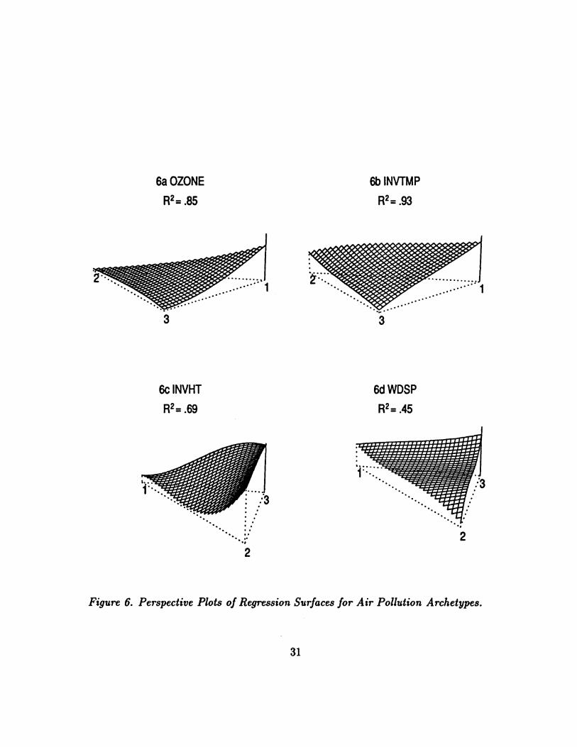
The surface plots of the five covariates, scaled in the same way as the ozone

surface plots are in Figure 13 a) - e). Because there are only 40 data points, the

regression used only the linear and quadratic terms in the mixture coefficients giving

5 independent variables.

The R2 were

* ESF .71

* LPC .44

* TMF .24

* LVG .19

* LPD .07

Given that we are using 40 cases and 5 variables, some of these R2 are substantial.

The surface plots show that the archetypes and the covariates are associated as

follows

12

Archetype ESF LPC TMF LVG

1 low high moderate high

2 low moderate low moderate

3 high low high low

This archetypal analysis gives some new and interesting insights into the rela-

tionships between the temperature profiles and the covariates. Much more extensive

statistical work needs to be done in this area.

3. LOCATION OF THE ARCHETYPES

The following proposition helps in understanding the nature of archetypes.

PROPOSITION 1. Let C be the convex hull of ,,... , 7. Let S be the set of data

points on the boundary of C and let N be the cardinality of S.

(i) If p = 1, choosing z to be the sample mean minimizes RSS.

(ii) If 1 < p < N, there is a set of archetypes {z1,..., zp} on the boundary of C which

minimize RSS.

(iii) If p = N, choosing {z1,... , zp}= S results in RSS = 0.

Proof. In each case, it is easily verified that the proposed archetypes are mixtures

of the data. It remains to show that the archetypes minimize the RSS. For (i), the

sample mean is the unconstrained minimizer of the RSS. For (ii), suppose without

13

loss of generality that z1 is strictly interior to C, let

z(t) =z + t(zi -zj), for t > 1 andj #1,

and choose t so that z(t) is on the boundary of C. For zj,..., zp fixed, RSS is

minimized with respect to the a's by choosing FP 1 aikZk to be the point in the

convex hull of zj,..., zp that is closest to xi. But the convex hull of z(t), Z2,.. .,ZP

contains the convex hull of Z1,... ,Z ,P so z(t), z2,... , zp provide a larger set over

which to minimize (1) with respect to the a's. For (iii), the convex hull of z, ..., zp

is C, so RSS=O.

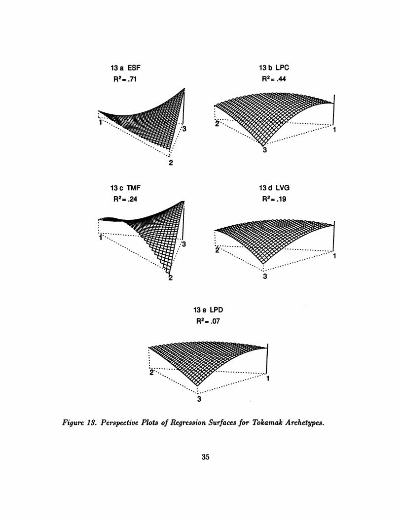
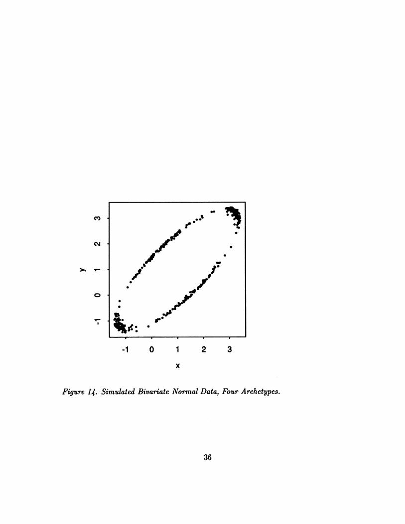
The editor raised the question of where the archetypes of simple distributions are

located. In general, the locations are quite data dependent, and sensitive to outliers.

Since analytic results seem formidable, the following simulation was done:

1) Generateasampleofsize1000fromN(s,E)where= ('),= ( ).

Discard any points outside the 95% density contour, i.e. with Mahalanobis Dis-

tance > X2(.95)

2) Fit 4 archetypes.

3) Repeat 100 times.

The plots of all archetypes are in Figure 14. They cluster around the ends of the

14

major and minor axes of the 95% density contour. This is what we expected, but its

comforting to get confirmation.

4. THE ARCHETYPE ALGORITHM

Let z1, .. , zn be n m-dimensional data points. The problem is to find zl,. .. , zp

wheren

Zk E= kjZjj=1

and z1, .. . ,zp minimize

RSS=minZE x~i-ZCikZk(41{ca,k) =1 k=1

subject to the constraints

a,ik.> for i =1,...,n; k=,...,pp

Eaik=l for i=1,...,nk=1

flk.>O for k=1,...,p; j ,...,nn

Z Pki=1 for k =,...,p.

The Zk's are the archetypes; the algorithm used to compute them will be called

the archetype algorithm.

The residual sum of squares in (4.1) can be written

74 p n2

RSS =E xi-ZE fikZEfkjj, |i=1 k=1 j=1

15

and the archetype problem is to find a's and I's to minimize this RSS subject

to the constraints above. This problem could be solved using a general-purpose

constrained nonlinear least squares algorithm, but this may prove impractical for

all but the smallest problems. Instead, we propose an alternating constrained least

squares algorithm.

4.1 Alternating Optimization

The algorithm alternates between finding the best a's for a given set of x-mixtures,

and finding the best x-mixtures for a given set of a's. Each step requires the solution

of several convex least squares (CLS) problems of the form

Given u andt1.l.., tq, find wl,...,wq to minimize Ilu - 1k w 1ktkI2 sub-

ject to wU O> 0 for k = 1,...,q and Eq= WIk=1.

At each step, the sum of squares (4.1) is reduced, and the algorithm stops when

the reduction is sufficiently small.

First consider finding the best a's for a given set of x-mixtures z, ...., zp. Finding

the best a's requires the solution of n CLS problems, namely, minimizing

p 2

xi - E ztikZk

for each i, subject to ai,k > 0 for k = 1,... ,p and EP=, ai, = 1. Each of the n CLS

problems has m observations and p variables.

16

Now consider finding the best x-mixtures for the current set of a's. If all but one

of the x-mixtures are held constant, we show that the remaining one can be found by

solving a CLS problem. More precisely, if zx is the x-mixture of interest, let

Vi (xi- ZaikZk) /ailn /n

E at21Vi /Eti21i= i=

and write (4.1) as

n12 lVi Z 112

i=ln n

= tEi2 liVi _V112 + ECz2t IIV Z 112.i=l i=l

Since the first term does not depend on zl, minimizing f is equivalent to minimizing

IIv-Z1112 = IIi;-2._Ejn 1,6z,112, subject to the constraints f83i .0 for j = 1,... , n and

Z7=1,81 = 1, which is a CLS problem with n variables and m observations.

The entire collection of x-mixtures is found by cycling through the set, optimizing

with respect to each x-mixture in turn, until the improvement in the objective function

from an entire pass is smaller than some prescribed tolerance. The resulting x-

mixtures are the archetypes.

4.2 Implementation

Many methods are available for solving CLS problems. The method used to

develop and test the algorithm is a penalized version of the NNLS algorithm in Lawson

17

and Hanson (1974). In particular, we obtain ui and t1,... , tp by adding an extra

element M to u and tj, ... ,tp, where M is large. Then

2 2 2

u - Wktk = U->ZWktk +M2 1-1EWkk=1 k=1 k=1

which is minimized under non-negativity restrictions. For large M, the second term

dominates and forces the equality constraint to be approximately satisfied, while

maintaining the non-negativity constraint. The speed of the archetype algorithm is

determined by the efficiency of the CLS method. The penalized non-negative least

squares method is appealing because it can be used when the number of variables is

larger than the number of observations. However, it is still quite slow, and alternative

convex least squares procedures are being developed (Cutler 1993).

Initially, the x-mixtures may be chosen at random without replacement from the

data. Some caution should be exercised in choosing initial x-mixtures that are not

too close together, since this can cause slow convergence or convergence to a local

optimum.

At any stage, if one or more of the x-mixtures is inside the convex hull of the

others, E.nL can be zero. When this occurs, the archetype is redundant and may

be replaced by that data point xi for which lmi - Ek=l aikZk112 is the largest.

5. CONVERGENCE

As with many alternating optimization algorithms, the archetype algorithm can

18

be shown to result in a fixed point of an appropriate transformation, but there is no

guarantee that this will be a global minimizer of RSS.

First consider the inner loop used to compute the 8's. Let

0 - l($ ,* *X ln ..v v,pl) ..* * pn)t

)---I.. bn)

for bk = (fkl,. ..,kn)t The inner loop produces iterates 01,82'... by minimizing

(1) with respect to the current bk while holding the others fixed. This gives f(i31) <

f032) < ..., and since the set B of feasible 's is compact, the iterations for the inner

loop have a limit point 3*.

Treating RSS in (4.1) as a function of ,3 gives

n

f(3) = ZitTi- 2ct3 + 3tH,3i=1

where c = (Cll...,C1n7 ... .p Cp,)t for ck = Cikait:j and H XtX AtA,

where A has i, k element aik, X= (X17 ... , On), and 0 denotes the direct product.

Since XtX and AtA are both positive semi-definite, H is also positive semi-definite,

so f is a convex function of /3.

PROPOSITION 2. The limit point ,3* minimizes f over B.

Proof. If g : A -+ R is a convex continuously differentiable function and A is a con-

vex subset of Rq, then g has a global minimum at y* E A iff Vg(y*)t(y -y*) > 0 V y E

A. Let ( ,tn)for i = 1, . . . ,pandfk(b) = f(bl*,,. . .,b**_Ib,b*+1b1).19

Then fk : B1 R is a convex continuously differentiable function and B1 = {b E Rn:

bi > 0 and EX bi= 1} is compact. Since b* minimizes fk over B1, Vfk(b*)t(b-b*) >0 v b E B1. But Vf(,3*)t (vfi(bl*)t, ... Vfp(b*), so

pVf(/3' )t(,f3- 3*) = Vfk(b*)t(bk - b*) 2 0

k=1

v P3 = (bt1... bt)t E B1 x ... x B1 = B, and since f is convex, this implies that /3*

minimizes f over B.

PROPOSITION 3. If A has rank p, then the x-mixtures z1,.. ., zp which minimize

(4.1) for fixed a's are unique.

Proof. Let zt = (zt,.,. zt) and treat f as a function of z. Then

n

f(z) E .it -i 2dtz + ztGzi=1

where dt = (dt,... , dt) for dk = Z aikTi&, G = Im 0 AtA, and Im denotes the m

by m identity matrix. Since A has rank p, G is positive definite so f(z) is strictly

convex. Now f is minimized over a convex set, so the constrained problem has a

unique minimum.

Propositions 2 and 3 establish the convergence of the inner loop to x-mixtures

that minimize (4.1) for fixed a's. Although the ,B's might not be unique, the corre-

sponding x-mixtures are unique. That the a's minimize (1) for fixed x-mixtures is

immediate. These results do not imply that the alternating optimization algorithm

invariably converges to the global minimum of (4.1). Numerical experiments suggest

20

Table 1. Local Minima and Timings

Data Set n m p Trials until Percentage CPU sec

global min local min per trial

Masks 200 6 2 1 0 1.5

3 2 27 2.5

4 1 51 4.5

5 5 73 5.8

Pollution 330 9 2 1 0 2.2

3 1 0 4.0

4 1 30 8.5

5 1 45 13.4

Tokamak 40 35 2 1 0 1.4

3 2 37 1.5

4 3 73 2.2

5 3 76 4.1

21

that convergence to local minima or other stationary points becomes more of a prob-

lem as the number of archetypes required increases. For example, in the Swiss Army

mask data, in 1000 random starts for computing two archetypes, all converged to the

same solution.

But local minima problems occurred in computing 3 or more archetypes. To see

the extent of the problem, 500 random starts were used in computing 2, 3, 4, and 5

archetypes for the mask data. This was repeated for the air pollution and Tokamak

data discussed in Section 2.

The results are given in Table 1. The fifth column gives the number of trials until

the global minimum was first found, the sixth column gives the percentage of times

local minima were found in the 500 trials, and the last column gives the average CPU

seconds per trial on a SPARC 10 processor.

All examples given in this paper have been validated as global minima through the

use of repeated random starts.

6. CONCLUDING REMARKS

Archetype analysis gives a simple and useful way of looking at multivariate data.

Archetypes are relatively easy to interpret and the mixture coefficients can provide

interesting information about the structure of the data. Past this, the examples speak

for themselves.

Sometimes the variables used in the analysis should be standardized before com-

22

puting archetypes - sometimes not. The Swiss head dimension and air pollution data

were standardized, but not the Tokamak data. When to use standardization depends

on one's sense about the data.

Since the archetypes are located on the boundary of the convex hull of the data,

the procedure can be sensitive to outliers. Robust versions could be developed using

convex hull peeling or the outlyingness idea of Donoho and Gasko (1992).

In the more serious examples, we worked with 3 archetypes getting various graph-

ical displays such as the mixture triangles and surface plots. Suppose that more

than 3 archetypes are needed for a reasonable approximation to the data. We think

that analogous graphical displays can be made using an appropriate mapping of the

archetypes to the plane. Some experimentation has been done along these lines with

encouraging results, but we leave the issue to future work.

The FORTRAN code for archetype analysis and an interface to S is available from

the first author or electronically from adele@sunfs.math.usu.edu. The authors would

like to thank Mark Hansen for suggesting the displays in Figures 5 and 12, and Mike

Windham for suggestions and discussions relating to this work.

Kurt Riedel was of invaluable assistance in guiding us through the Tokamak maze,

and transmitted the data we used. Thanks are also due to Ken Fowler (UCB Physics

Department) and Mort Levine (Lawrence Berkeley Lab (ret)) for trying to educate

us about Tokamaks.

23

REFERENCES

Breiman, L. and Friedman, J.H. (1985), "Estimating Optimal Transformations in

Multiple Regression and Correlation," JASA, V.80, No. 391, 580-619.

Cutler, A. (1993), "A Branch and Bound Algorithm for Convex Least Squares,"

Communications in Statistics: Simulation and Computation, V.22, No. 2, 305-

321.

De Leeuw, J. and van der Heijden, P.G.M. (1991), "Reduced Rank Models for Con-

tingency Tables," Biometrika, V.78, No. 1, 229-232.

Donoho, D.L. and Gasko, M. (1992), "Breakdown Properties of Location Esti mates

Based on Halfspace Depth and Projected Outlyingness," The Annals of Statis-

tics, V.20, No. 4, 1803-1827.

Flury, B. (1990), "Principal Points," Biometrika, 77, 33-41.

Flury, B. (1993), "Estimation of Principal Points," Applied Statistics, V.42, No. 1,

139-151.

Flury, B. and Riedwyl, H. (1988), "Multivariate Statistics, A Practical Approach"

London: Chapman and Hall.

Flury, B. and Tarpey, T. (1992), "Representing a Large Collection of Curves: a Case

for Principal Points," Unpublished Manuscript.

24

Hastie, T. and Tibshirani, R. (1990), Genealized Additive Models, Chapman and

Hall.

Hiroe, A. et al. (1988), "Scale Length Study in T.F.T.R.," Princeton Plasma Physics

Laboratory Report #2576.

Jones, M.C. and Rice, J.A. (1992), "Displaying the Important Features of Large

Collections of Similar Curves," The American Statistician, 46, 140-145.

Kardaun, O.J.W.F. Riedel, K.S. et al (1990), "A Statistical Approach to Plasma

Profile Analysis," Max-Plank-Institut fuir Plasmaphysic, IPP 5/35.

Lawson, C.L. and Hanson, R.J. (1974), Solving Least Squares Problems, New Jersey:

Prentice-Hall.

Lazarsfeld, P.F. and Henry, W. (1968), Latent Structure Analysis, Boston: Houghton

Mifflin.

McCarthy, P.J., Riedel, K.S. et al (1991), "Scalings and Plasma Profile Parameter-

ization of Asdex High Density Ohmic Discharges," Nuclear Fusion, V.31, No.

9, 1595-1633.

Riedel, K.S. and Imre, K. (1993), 'Smoothing Spline Growth Curves with Covari-

ates," Communications in Statistics: Theory and Methods, V.22, No. 7, 1795-

1818.

25

van der Heijden, P.G.M., Mooijaart, A. and De Leeuw, J. (1992), "Constrai ned

Latent Budget Analysis," Sociological Methodology, 22, 279-320.

Woodbury, M.A. and Clive, J. (1974), "Clinical Pure types as a Fuzzy Part ition,"

Journal of Cybernetics, V.4, No. 3, 111-121.

26

4

2

5

6 3*.......*I

Two Archetypes

Three Archetypes

FcI

Four Archetypes

(I).*

Five Archetypes

I _ i

Figure 1. Archetypes for Head Dimension Data.

27

LI1

I

I

p

Figure 2. Percent RSS for Swiss Army Archetypes.

'o8

_r aO

x

8 sB'V

1 2 3 4 5

p

Figure 3. Percent RSS for Air Pollution Archetypes.

28

0

0

0

4, 0

0

0

0

5I 2 3 4

Archetype 1

/2 /A/A VIA II / Ir7zOZONE 500MH WDSP HMDTY STMP INWHT PRGRT INVTMP VZBLTY

Archetype 2

OZONE 50OMH WDSP HMDTY STMP INVHT PRGRT INVTMP VZBLTY

Archetype 3

7771

OZONE 500MH WDSP HMDTY STMP INVHT PRGRT WIVTMP VZBLTY

Figure 4. Percentile Profiles of Air Pollution Archetypes.

29

0O'

0o

0I0

0,

0

0

0to0

0

0

00

0

0

0

CD

- - - - . - - --. - - - . A - - - 1- - W- .r le i r-lw--N.-9n Iizzzi v z z I I Z z ziJLAL-AL-Z--L-

....... -

P7,A f--r-Y-71 I

5a Spring2

. 00'a .

* 0

* 00

0

000. 0~~~~ *

*0 &#S1'a ,s .,* "

1t 13

5c Fall2

/ 0a*

* 0

* *001* 0-

* ~~* :* *0.0

- * S * * :

0...p..-1 ....... 3

1

5b Summer2

* .

* 0

0 000.* 0*0X

* @~~~

5d Winter2

0

o* *0* *00

0

10 00 0

0 00 0000* 0 *oe~0 0

0D 00 0 00

0 0 A.-....... ..-.. . ..

3

Figure 5. Mixture Plots for Air Pollution Archetypes.

30

.. 0

6a OZONER2= .85

6b INVTMPR2= .93

3 3

6c INVHTR2= .69

6d WDSPR2= .45

2

p..3.::--. .

. . .

2

Figure 6. Perspective Plots of Regression Surfaces for Air Pollution Archetypes.

31

Raw Temperature Curves

E: 0

rcJ

2.0 2.2 2.4 2.6 2.8 3.0 3.2

raius

Figure 7. Raw log(Temperature) against radius.

Smoothed Temperature Curves

2.0 2.2 2.4 2.6 2.8 3.0 3.2

raius

Figure 8. Smoothed log(Temperature) against radius.

32

Vo.0

WO

£ °

Normalized Temperature Curves

la.

Wa

0

-

cci

0

ci

2.2 2.4 2.6 2.8 3.0

radius

Figure 9. Normalized, smoothed, log(Temperature) against radius.

08

x

0

1 2 3 4 5

p

Figure 10. Percent RSS for Tokamak Archetypes.

33

IL

2.8 3.0

radius

Figure 11. Three Archetypal Curves, Tokamak data.

2. .

0

;; *-

0

0 0

* *

* *

*..'..O O wo T0.....* 4

1 3

Figure 12. Mixture Plot for Three Tokamak Archetypes.

34

3 Archetypes

go.I

v-

c

0o.

2.2 2.4 2.6

210e ,.0-1 I

-ft.:--.. .

/. .- I

, , , , , ,, S.*

..IV.

-b0 IX

& .I\0

1

0

I

13 a ESF 13 b LPCR2=.71 R2=

2

13 c TMF 13 d LVGR2=.24 R2=.19

3

13e LPDR2= .07

.............

3

Figure 13. Perspective Plots of Regression Surfaces for Tokamak Archetypes.

35

0

1

0

.*I@0

_0

I0

.

0 1 2 3

x

Figure 14. Simulated Bivariate Normal Data, Four Archetypes.

36

CO

cMJ

0