area reduction of syndrome calculator for …eprints.usm.my/41305/1/koay_kim_leong_24_pages.pdf ·...
TRANSCRIPT

i
AREA REDUCTION OF SYNDROME CALCULATOR FOR STRONG
BOSE-CHAUDHURI-HOCQUENGHEM DECODER
By
KOAY KIM LEONG
A Dissertation submitted for partial fulfilment of the requirement for the degree
of Master of Microelectronic Engineering
August 2016

ii
ACKNOWLEDGEMENTS
First of all, I would like to say my deepest gratitude to my supervisor, AP Dr.
Bakhtiar Affendi bin Rosdi for his guidance and patient capacity to improve the quality
of this project. His advice and support lead me to the right path in completing this
research project. I am pleased to be under his supervision. He guided me in conducting
a proper research.
Next, I would like to thank my colleague PJ Tan for his extra time in ramping
up me on operating the EDA tools for this research.
Last but not least, with my heartiest gratitude, I thank my wife for all her
supports and extra time spent on our daughter in order to free me up for my academic
life since the very beginning of this course. Without her, this thesis I would not be the
same as presented here.
iii
TABLE OF CONTENTS
ACKNOWLEDGEMENTS .................................................................................................................... ii
TABLE OF CONTENTS ....................................................................................................................... iii
LIST OF TABLES ................................................................................................................................. v
LIST OF FIGURES .............................................................................................................................. vi
LIST OF ABBREVIATIONS ................................................................................................................ vii
ABSTRAK ....................................................................................................................................... viii
ABSTRACT ....................................................................................................................................... ix
CHAPTER 1 ....................................................................................................................................... 1
1 INTRODUCTION ........................................................................................................................ 1
1.1 Background ......................................................................................................................... 1
1.2 Problem Statements ........................................................................................................... 3
1.3 Objectives ............................................................................................................................ 4
1.4 Research Scope ................................................................................................................... 5
1.5 Thesis outline ...................................................................................................................... 5
CHAPTER 2 ....................................................................................................................................... 7
2 LITERATURE REVIEW ................................................................................................................ 7
2.1 Introduction ........................................................................................................................ 7
2.2 Error correction codes (ECC) ............................................................................................... 7
2.3 Galois Field (GF) ................................................................................................................ 10
2.3.1 Properties of Galois Fields ....................................................................................... 11
2.3.2 Binary field GF(2) ..................................................................................................... 11
2.3.3 Extended Binary Field GF(2m) .................................................................................. 12
2.3.4 Representation of Galois Field Elements ................................................................. 14
2.4 BCH Code ........................................................................................................................... 14
2.4.1 BCH Code Construction ........................................................................................... 16
2.4.2 Syndrome Calculation (SC) ...................................................................................... 17
2.4.3 Computation of Error Locator Polynomial ............................................................... 18
2.4.4 Berlekamp-Massey Algorithm (BMA) ...................................................................... 20
2.4.5 Chien Search (CS) ..................................................................................................... 24
2.5 Conventional Syndrome Calculation Architecture ............................................................ 25
2.5.1 Serial syndrome calculation ..................................................................................... 25
iv
2.5.2 Parallel syndrome calculation .................................................................................. 26
2.5.3 Parallel syndrome calculation with power operation.............................................. 27
2.5.4 Parallel syndrome calculation with input XOR ........................................................ 29
2.6 Summary ........................................................................................................................... 30
CHAPTER 3 ..................................................................................................................................... 32
3 METHODOLOGY ..................................................................................................................... 32
3.1 Introduction ...................................................................................................................... 32
3.2 Development of an architecture of the SC block for BCH (n=255, k=111, t=18) decoder 33
3.3 RTL implementation of the developed architecture ......................................................... 41
3.4 Performance evaluation of the RTL implementation ........................................................ 43
3.5 Summary ........................................................................................................................... 45
CHAPTER 4 ..................................................................................................................................... 47
4 RESULTS AND DISCUSSION ..................................................................................................... 47
4.1 Introduction ...................................................................................................................... 47
4.2 Simulation results of RTL design ....................................................................................... 48
4.3 Logic synthesis results of RTL design ................................................................................. 53
4.4 Summary ........................................................................................................................... 55
CHAPTER 5 ..................................................................................................................................... 57
5 CONCLUSION AND FUTURE WORK......................................................................................... 57
5.1 Conclusion ......................................................................................................................... 57
5.2 Future work ....................................................................................................................... 58
REFERENCES ................................................................................................................................... 60
APPENDICES ................................................................................................................................... 64
Appendix A: RTL coding of BCH decoder with SC block architecture proposed in [8]
Appendix B: RTL coding of BCH decoder with SC block architecture proposed in current research
Appendix C: Area consumption report of BCH decoder with SC block architecture proposed in [8]
Appendix D: Area consumption report of BCH decoder with SC block architecture proposed in
current research
Appendix E: Power consumption report of BCH decoder with SC block architecture proposed in [8]
Appendix F: Power consumption report of BCH decoder with SC block architecture proposed in current
research

v
LIST OF TABLES
Table 2-1 Modulo-2 addition of two elements, A and B in GF(2) ............................ 12
Table 2-2 Modulo-2 multiplication of two elements, A and B in GF(2) ................... 12
Table 2-3 GF(23) generated by the primitive polynomial 𝑝(𝑋) = 𝑋3 + 𝑋2 + 1 over
GF(2) .................................................................................................................. 14
Table 2-4 BMA execution table ................................................................................. 22
Table 2-5 Simplified BMA execution table ............................................................... 23
Table 2-6 Comparison of SC block architectures ...................................................... 31
Table 3-1 Power operation of odd-index syndrome with n=255 ............................... 37
Table 3-2 Power operation of odd-index syndrome with n=255, t=18 ..................... 37
Table 3-3 Characteristics and architectures of BCH decoders implementation ........ 40
Table 3-4 Test vector used for functional verification ............................................... 43
Table 4-1 Comparison of area and power consumption in between proposed SC
block vs previous work ...................................................................................... 55

vi
LIST OF FIGURES
Figure 2-1 Basic digital communication system block diagram .................................. 8
Figure 2-2 Typical BCH encoding and decoding operation ...................................... 16
Figure 2-3 Basic syndrome calculator unit ................................................................ 25
Figure 2-4 Conventional p-parallel syndrome calculation unit [8] [22] .................... 26
Figure 2-5 Even-index syndrome computed by power operation for BCH decoder
with t=6 .............................................................................................................. 28
Figure 2-6 Basic Circuit of D-Flip-Flop with Set and Reset [32] .............................. 29
Figure 2-7 Basic Circuit of two inputs XOR logic gate [33] ..................................... 29
Figure 3-1 Three main development phases .............................................................. 32
Figure 3-2 Conventional p-parallel SC unit [22] ....................................................... 33
Figure 3-3 Flowchart of the odd-index syndrome selection to be computed by using
power operation .................................................................................................. 36
Figure 3-4 Syndrome that can be computed by power operation for BCH (n=255,
t=18) decoder proposed in [8]. .......................................................................... 39
Figure 3-5 Syndrome that can be computed by power operation for BCH (n=255,
t=18) decoder proposed in this research project ................................................ 39
Figure 3-6 Hierarchical structure of the RTL implementation of the BCH decoders 41
Figure 3-7 Block diagram of the RTL implementation of BCH decoder .................. 44
Figure 4-1 BCH decoder from [8] is able to correct 1 bit error ................................. 49
Figure 4-2 BCH decoder from [8] is able to correct 8 bit errors ............................... 50
Figure 4-3 BCH decoder from [8] is able to correct 18 bit errors ............................. 50
Figure 4-4 BCH decoder from [8] is unable to correct 19 bit errors.......................... 50
Figure 4-5 BCH decoder of current work is able to correct 1 bit error ...................... 51
Figure 4-6 BCH decoder of current work is able to correct 8 bit errors .................... 51
Figure 4-7 BCH decoder of current work is able to correct 18 bit errors .................. 51
Figure 4-8 BCH decoder of current work is unable to correct 19 bit errors .............. 52
Figure 4-9 S9 and S25 computation of BCH decoder from [8] ................................... 52
Figure 4-10 S9 and S25 computation of BCH decoder of current work ..................... 53

vii
LIST OF ABBREVIATIONS
ARQ Automatic Repeat Request
BCH Bose–Chaudhuri–Hocquenghem
BM Berlekamp-Massey
BMA Berlekamp-Massey Algorithm
CS Chien Search
ECC Error Correction Code
EDA Electronic Design Automation
FEC Forward Error Correction
GF Galois Fields
HDL Hardware Description Language
LCM Least Common Multiple
LDPC Low-Density Parity-Check
MLC Multi-Level Cell
RS Reed-Solomon
RTL Register Transfer Logic
SC Syndrome Calculation or Syndrome Calculator
SLC Single Level Cell
SSD Solid-State Drives
SV System Verilog
VCS Verilog Compiler Simulator
WBAN Wireless Body Area Network
XOR Exclusive OR

viii
PENGURANGAN KELUASAN KALKULATOR SINDROM UNTUK
DEKODER BOSE-CHAUDHURI-HOCQUENGHEM YANG KUAT
ABSTRAK
Kod Bose–Chaudhuri–Hocquenghem (BCH) mempunyai penggunaan yang meluas
untuk memberi perlindungan ralat untuk berbilang ralat rawak dalam kod binari. Ini
merupakan faktor penting untuk menggunakan Kod BCH biasanya digunakan dalam
pelbagai aplikasi seperti “solid-state drives” (SSDs) dan sistem komunikasi gentian
optik berkelajuan tinggi, sistem komunikasi tanpa wayar. Operasi dalam dekoder BCH
boleh dirumuskan kepada 3 langkah: 1) mengira sindrom daripada kod diterima; 2)
pengiraan polinomial pengesanan ralat; 3) mengesan ralat daripada kod diterima.
Projek penyelidikan ini mencadangkan blok kalkulator sindrom yang cekap untuk
BCH (n = 255, k = 111, t = 18) dekoder dari segi penggunaan keluasan perkakasan.
Dalam seni arkitek blok kalkulator sindrom sebelumnya, semua sindrom ganjil perlu
dikira dengan pengiraan langsung yang memerlukan lebih keluasan. Dalam seni
arkitek yang dicadangkan, ciri-ciri Galois field telah dieksploitasi untuk mengira
sindrom ganjil dengan menggunakan kaedah operasi kuasa untuk menjimatkan
penggunaan keluasan. Seni arkitek yang dicadangkan adalah lebih baik dari segi
penggunaan keluasan berbanding dengan seni arkitek sebelumnya. Kesimpulannya,
dengan mengira sindrom ganjil indeks dengan operasi kuasa, 8% penjimatan keluasan
dicapai tanpa menjejaskan penggunaan kuasa dan frekuensi operasi.
ix
AREA REDUCTION OF SYNDROME CALCULATOR FOR STRONG
BOSE-CHAUDHURI-HOCQUENGHEM DECODER
ABSTRACT
Bose–Chaudhuri–Hocquenghem (BCH) codes have a widespread use to provide the
error protection for multiple random errors in a binary code. BCH codes is commonly
applied in various practical application such as advanced solid-state drives (SSDs),
high-speed fiber optical communications system and wireless communication system.
The operation in a BCH decoder can be summarized into 3 steps: 1) compute the
syndromes from the received codeword; 2) computing the error locator polynomial; 3)
locating the errors. This research project proposed an area efficient Syndrome
Calculator block of the BCH (n=255, k=111, t=18) decoder. In the previous SC block
architecture, all the odd-index syndromes need to be computed by direct calculation
which consume more area. In the current proposed architecture, Galois field’s property
is exploited to compute the odd-index syndromes by using power operation in order to
save the area consumption. This architecture is better in terms of area compared with
previous architecture. In conclusion, by computing the odd-index syndromes with
power operation, 8% area saving is achieved without compromising the power
consumption and its operating frequency.

1
CHAPTER 1
1 INTRODUCTION
1.1 Background
Error-correction codes (ECC) are techniques that provide the delivery of digital
data reliably over an unreliable communication channels. Many communication
channels are subject to noise and interference. Errors may be introduced from the
source to the receiver during transmission. Error detection techniques enable the
detection of such errors, while error correction allow restoration of the original data in
many cases. ECC have a widespread use in communication systems to recover errors
caused by poor environment. There are many types of ECC such as Hamming codes,
Bose–Chaudhuri–Hocquenghem (BCH) codes, Reed–Solomon (RS) codes, turbo
codes and low-density parity-check codes (LDPC). Hamming codes is one of the
earliest ECC [1] [2] [3]. BCH codes and RS codes are among the most popular codes
due to their widespread use in current communication systems [1] [2] [3]. Turbo codes
and LDPC codes are relatively new constructions that can provide almost optimal
efficiency [1] [2].
BCH codes is one of the most commonly applied error-correction code in many
communication system. For instance, BCH codes applied to one of the standard that is
most common choices in Digital TV broadcasting system [4] [5]. Besides, BCH codes
is chosen to be implemented in Wireless Body Area Network (WBAN) for its low
power consumption advantage [6]. Recent years, BCH codes is applied to

2
cryptographic hardware designs that need to store some high security information as
well. This because the occurrence of malicious attack increases drastically due to the
widespread usage of online activities globally [7].
Apart from that, recent applications of data storage system such as advanced
solid-state drives (SSDs) are heavily rely on BCH code to correct the errors occurred
in the memory cell [8] [9]. High demand for increased storage capacity has resulted in
the introducing multi-level cell (MLC) from single level cell (SLC) to reduce the
production cost. However, MLC is experiencing higher error rate as compared to
previous SLC. BCH codes are added to detect and correct the error introduced in the
storage devices. High speed BCH decoding performance and high error-correction
capability are greatly demanded. Massive parallel BCH decoding is able to satisfy such
a high-throughput and high error correction requirement by paying the additional cost
to the area consumption. However, larger area resulted higher power consumption and
lower die utilization of the storage devices. Therefore, a strong and high performance
but yet small size of BCH decoder is required to overcome the issue. A BCH decoder
is considered strong if it can correct 5 or more errors [31].
BCH codes is popular for its capability to correct multiple random error in a
binary code. Also, BCH codes is known to be cost effective, reliable, flexibility and
most importantly its simplicity in implementation [10]. BCH codes are cyclic codes
which work under Galois Field (GF). The Galois fields or Finite fields’ theory defines
the properties of BCH codes. In general, development of a BCH decoder can be
summarized into three steps: 1) syndromes calculation (SC) from the received
codeword; 2) computing the error locator polynomial by using Berlekamp-Massey
algorithm (BMA); 3) finding the error locations by applying Chien Search (CS).

3
In this project, syndrome calculation from the received codeword is carried out
by the combination of direct computation and power operation in binary Galois fields.
The direct computation unit is comprising of p-parallel syndrome calculation unit
which process p-bit of codeword in an iteration. Power operation in binary Galois
fields unit consist of a series of XOR logic gates. For computing the error locator
polynomial, inversion-less BMA is chosen [11] to eliminate the complex calculation
of inverses in Galois fields. Lastly, for the sake of area consideration, the conventional
serial Chien Search [1] is selected to find the error locations.
1.2 Problem Statements
In order to increase the performance of the decoder, each sub-block of a BCH
decoder can be implemented with a large parallel factor. Several optimization schemes
have been developed for the Chien search to increase its performance as well as
reducing the area consumption [12] [13]. On the other hand, there are several
enhancement proposed by researchers to relax the complexity of a BMA design. For
example, BMA architecture proposed in [14] reduces the area consumption, while
BMA architecture proposed in [15] reduces the latency of the BMA block. In terms of
SC block, performance of calculation was improved by implementing the parallel
syndrome calculation unit in the SC block. This is to reduce the number of iterations
required to calculate all the syndromes.
Error correcting capability of BCH decoder is also affecting the area
consumption of the design. However, SC block is the one that mainly impacted
because more parallel syndrome calculation units required to calculate all syndromes.

4
The SC block in [8] proposed to exploit Galois fields’ property to compute the even-
index syndromes from odd-index syndromes by power operation. Result shown
signification improvement of more than 50% of area reduction. One year later, the
same group of researchers proposed another innovation to further reduce the area
consumption around 10% - 20% by eliminating the duplicate calculation of the
common sub-expression (CSE) of GF multiplication [16]. Even though both of the
proposed architectures shrink the area consumption significantly, still the direct
computation syndromes are required for all of the odd-index syndromes.
The specific focus area of the project is a continuous research to develop a new
architecture to decrease the number of direct computation of the syndrome in the SC
block. This is to further reduce the area of an SC block for a strong BCH decoder while
not sacrificing its decoding performance.
1.3 Objectives
The objectives of the research project are as follows:
1. To propose a better architecture to reduce the area consumption of the SC block
of a BCH decoder without sacrificing its performance.
2. To implement the proposed architecture into a RTL and synthesize the design
to obtain the area report in order to justify the result.

5
1.4 Research Scope
The scope of this research project consists of:
1. Review of the previous state-of-the-art of the BCH SC block.
2. RTL implementation and simulation of the BCH decoder with the
proposed architecture of new SC block by using System Verilog (SV)
Hardware Description Language (HDL). The RTL design is verified by
using Synopsys VCS simulator.
3. RTL logic synthesis of the design for comparison in between the proposed
architecture and the previous BCH decoder. The logic synthesis process
is carried out by using Synopsys Design Compiler tools.
4. The proposed architecture mainly focus on the area optimization of the
SC block in a BCH decoder without compromising its performance and
power consumption.
1.5 Thesis outline
This thesis consists of five main chapters.
In chapter 2, an overview of the BCH codes and its properties is presented and
Galois Fields will be discussed. Next, the general BCH encoder and decoder are
discussed. Then, the conventional architecture of the SC block and several
enhancements that have been proposed by other researchers on Syndrome Calculation
are discussed here as well.

6
Chapter 3 discuss the methodology of this research project in detail. First of all,
the proposed architecture of designing a small SC block is explained. Next, the details
design flow of the proposed architecture is described. The design languages that used
to implement the RTL and the tools that used to simulate and synthesis the design are
presented as well. The RTL architecture of the proposed SC block is explained in detail
and the comparison in between proposed method and the previous architecture are
presented. Subsequently, the test bench that used to verify the functionality of the
design is discussed. Lastly, the flow that used to justify the performance of the
proposed architecture is explained.
In chapter 4, the simulation results of the RTL design are presented and
discussed. Next, the logic synthesis results are analysed and discussed in various aspect
such as area consumption, power consumption and maximum operating frequency.
The simulation results and logic synthesis results are summarized in this chapter as
well.
Last but not least, chapter 5 gives the conclusion regarding the overall research.
Discussions and recommendations for future works on this project are highlighted as
well.
7
CHAPTER 2
2 LITERATURE REVIEW
2.1 Introduction
This chapter provides some basic concepts for better understanding of this
research. First of all, it is important to identify and understand the goal of this research.
Related researches on BCH code and current existing design architectures are
described in this chapter. This chapter begin with the basic introduction of ECC. Next
basic concept of Galois Fields that define the properties of BCH codes will be
presented. Subsequently, the overview of the BCH codes and its properties will be
discussed. In continuation with that, the conventional architecture of the SC block of
a BCH decoder and several enhancements that have been proposed by other
researchers on SC block are discussed as well.
2.2 Error correction codes (ECC)
Digital communication systems are very common in our daily lives. The most
common examples include cell phones, digital television, and digital radio and internet
connections [1]. Each of these examples are generally fits into a common digital
communication system block diagram as shown in Figure 2-1. The block diagram

8
shows two types of encoders and decoders, there are source encoder and decoder
together with channel encoder and decoder.
Source encoder converts the information source bit sequence into another bit
sequence with a more efficient representation of the information. This operation is
more often called compression. The source decoder is the encoder’s counterpart which
recovers the source sequence.
The function of the channel encoder is to protect the source sequence bits to be
transmitted over a noisy channel. The encoder converts its input into an alternate
sequence that provides immunity from the various channel impairments. On the other
side, the role of the channel decoder is to retrieve compressed sequence bits that input
to the channel encoder regardless of the presence of noise, distortion, and interference
in the received word from the channel output.
Figure 2-1 Basic digital communication system block diagram
There are huge number of channel coding techniques for the error prevention.
There are two main basic techniques namely automatic request-for-repeat (ARQ)
schemes and forward-error-correction (FEC) schemes [1]. In ARQ schemes, the
9
function of the code is simply to detect whether the received word contains any errors.
A request will be generated for retransmission of the same word from the receiver back
to the transmitter if a received word does contain one or more errors. This type of codes
are said to be error-detection codes. In FEC schemes, the code is capable to correct the
error detected through a decoding algorithm. The codes for this approach are said to
be error-correction codes (ECC).
ECC mechanism is implemented in two inverse operations, encoding and
decoding operation. The former operation is carried out by adding redundancy bits to
the message or information bits to form a longer binary sequence called codeword.
This operation is called encoding operation. The second operation is to retrieve the
message bits by excluding the redundancy bits from the received codeword. The
redundancy bits is often called parity check bits.
In block coding, an information sequence is segmented into message blocks of
fixed length. Each message block consists of k message bits and there are 2𝑘 unique
messages. At channel encoder, each input message sequence of k message bits is
encoded into an n-bits codeword with 𝑛 > 𝑘. Each codeword are one to one mapped
to each message. Since there are 2𝑘 distinct messages, there are 2𝑘 unique codewords
as well.
The codeword is more commonly represented in the form of (n, k) block code.
There are 𝑛 − 𝑘 parity check bits that are added to each input message sequence by
the channel encoder. The purpose of adding parity check bits is to provide the
codeword with the error detecting and error correcting capability. These parity check
bits do not carry any new information. The ratio, 𝑅 = 𝑘/𝑛 is called the code rate,
which is interpreted as the average number of information bits carried by each
codeword bit.

10
By definition [3] a binary (n, k) block code of length n with 2𝑘 codewords is
known as a linear (n, k) block code if and only if the 2𝑘 codewords form a k-
dimensional subspace of the vector space, 𝑉𝑛 of all the n-tuples over the field GF(2).
In another word, it may be seen that in a binary linear code, the modulo-2 sum of any
pair of code words generate another codeword.
There are many types of ECC such as Hamming codes, BCH codes, RS codes,
turbo codes and LDPC codes. BCH codes is one of the most popular codes for current
applications for its capability to correct multiple random error in a binary code,
effective, reliable, flexibility and most importantly its simplicity in implementation
[10]. BCH codes are cyclic codes which operate under Galois Field (GF). The Galois
Field’s theory defines the properties of BCH codes.
2.3 Galois Field (GF)
Galois field also known as finite field. It is the fields that contain finite numbers
of elements. Galois field play an important role in the construction of error-correction
codes that can be efficiently encoded and decoded. The set of integers, {0, 1, … , 𝑝 – 1},
forms a finite field GF(p) of order p under modulo-p addition and multiplication, where
0 and 1 are the zero and unit elements of the field.

11
2.3.1 Properties of Galois Fields
Some of the useful properties of a Galois field [1] are:
All elements in GF are defined on two binary operations which are addition
and multiplication.
Both addition and multiplication operations are commutative, associative,
and distributive.
The result of the binary operation must be an element in the GF.
The identity element of addition operation is called the “zero” element,
such that 𝑎 + 0 = 𝑎 for any element a in the field.
The identity element of multiplication is called the unit element, such that
𝑎 ∗ 1 = 𝑎 for any element a in the field.
For every element “a” in the GF, there is an inverse of addition element “b”
such that a + b = 0.
For every non-zero element “a” in the GF, there is an inverse of
multiplication element “b” such that 𝑎𝑏 = 1.
Subtraction can be defined as addition of the inverse whereas division can
be defined as multiplication by the inverse.
2.3.2 Binary field GF(2)
The simplest Galois field is GF(2). Its elements are the set {0, 1} under modulo-
2 addition and multiplication. Addition and subtraction are the same. The addition and

12
multiplication operation of two elements, A and B in GF(2) are shown in Table 2-1
and Table 2-2 respectively.
Table 2-1 Modulo-2 addition of two elements, A and B in GF(2)
Table 2-2 Modulo-2 multiplication of two elements, A and B in GF(2)
2.3.3 Extended Binary Field GF(2m)
The Galois field GF(2m) contains GF(2) as a subfield and is an extension field
of GF(2). Let us suppose 𝑞 = 2𝑚, for any positive integer m, a Galois field GF(q) with
q elements can be constructed based on the prime field GF(2) and the primitive element,
α of the GF(q). The power of 𝛼 are from 𝛼0 to 𝛼𝑞−2 and zero element from the GF(q).
It is given that,
𝛼2𝑚−1 = 𝛼0 = 1 (2.1)
Since addition and subtraction in GF(q) are the same, therefore,

13
𝛼2𝑚−1 + 1 = 0 (2.2)
Construction of Galois field GF(q) elements is based on irreducible primitive
polynomial denoted as p(X) with degree m, this polynomial need to be a factor of
𝑋2𝑚−1 + 1 [3]. For example, in GF(23) the factors of 𝑋7 + 1 are:
𝑋7 + 1 = (𝑋 + 1)(𝑋3 + 𝑋2 + 1)(𝑋3 + 𝑋 + 1) (2.3)
For both of the polynomials of degree 3 are primitive and irreducible that can be chosen.
Let us choose the polynomial shown in equation (2.1).
𝑝(𝑋) = 𝑋3 + 𝑋2 + 1 (2.4)
Let us suppose the primitive element α be the root of the primitive polynomial. By
substituting α into equation (2.4),
𝑝(𝛼) = 𝛼3 + 𝛼2 + 1 = 0 (2.5)
Rearranging equation (2.5), the equation can be represented as equation (2.6),
𝛼3 = 𝛼2 + 1 (2.6)
The other non-zero elements of GF(23) can be computed as:
𝛼4 = 𝛼 × 𝛼3 = 𝛼 × ( 𝛼2 + 1) = 𝛼3 + 𝛼 = ( 𝛼2 + 1) + 𝛼 = 𝛼2 + 𝛼 + 1 (2.7)
𝛼5 = 𝛼 × 𝛼4 = 𝛼 × ( 𝛼2 + 𝛼 + 1) = 𝛼3 + 𝛼2 + 𝛼 = 𝛼 + 1 (2.8)
𝛼6 = 𝛼 × 𝛼5 = 𝛼 × (𝛼 + 1) = 𝛼2 + 𝛼 (2.9)
𝛼7 = 𝛼 × 𝛼6 = 𝛼 × ( 𝛼2 + 𝛼) = 𝛼3 + 𝛼2 = 1 = 𝛼0 (2.10)
All the eight elements in GF(23) can be computed by the primitive polynomial
chosen from equation (2.4), are {0, 𝛼0, 𝛼1, 𝛼2, 𝛼3, 𝛼4, 𝛼5, 𝛼6}. All the elements
starting from 𝛼4 to 𝛼6 are presented function of 𝛼0, 𝛼1 and 𝛼2 which are called the
basis of the Galois field.
14
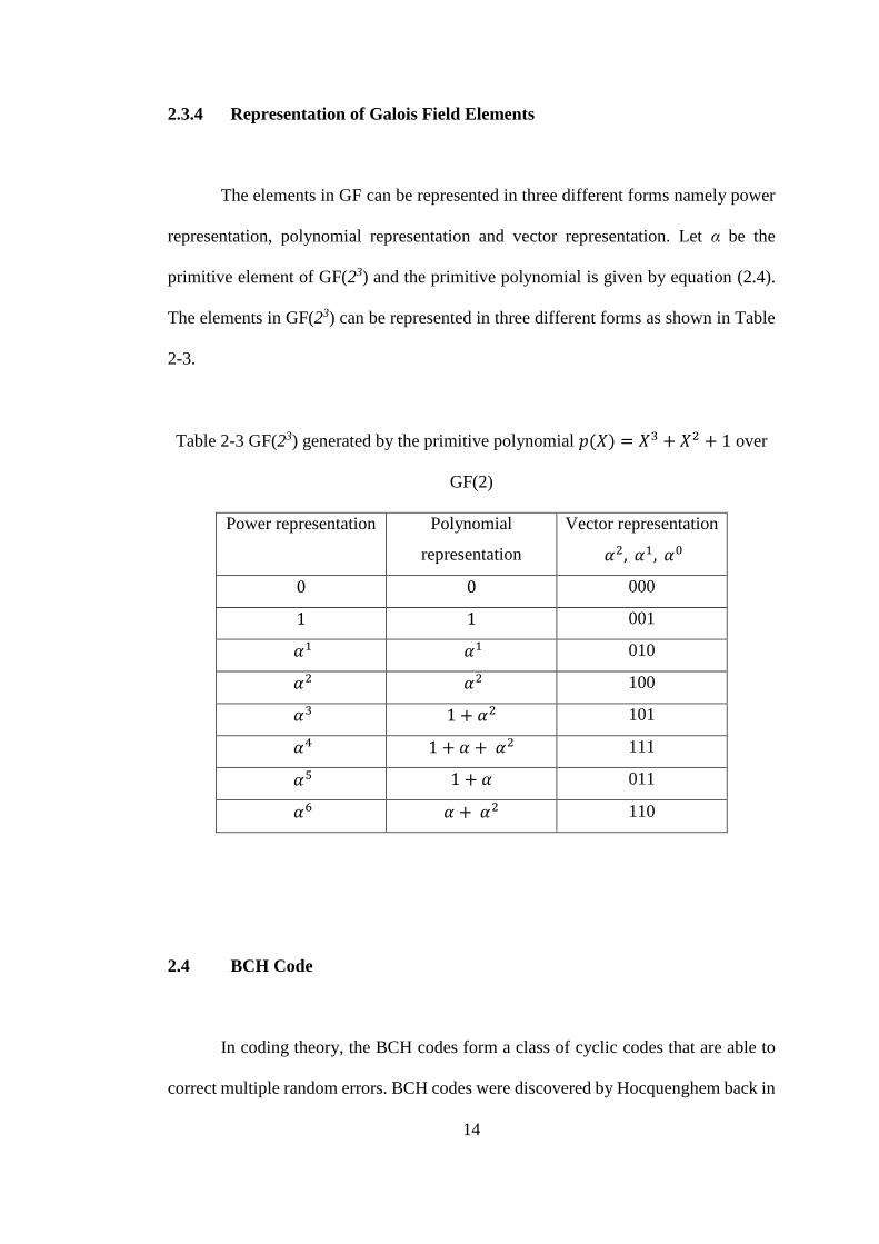
2.3.4 Representation of Galois Field Elements
The elements in GF can be represented in three different forms namely power
representation, polynomial representation and vector representation. Let α be the
primitive element of GF(23) and the primitive polynomial is given by equation (2.4).
The elements in GF(23) can be represented in three different forms as shown in Table
2-3.
Table 2-3 GF(23) generated by the primitive polynomial 𝑝(𝑋) = 𝑋3 + 𝑋2 + 1 over
GF(2)
Power representation Polynomial
representation
Vector representation
𝛼2, 𝛼1, 𝛼0
0 0 000
1 1 001
𝛼1 𝛼1 010
𝛼2 𝛼2 100
𝛼3 1 + 𝛼2 101
𝛼4 1 + 𝛼 + 𝛼2 111
𝛼5 1 + 𝛼 011
𝛼6 𝛼 + 𝛼2 110
2.4 BCH Code
In coding theory, the BCH codes form a class of cyclic codes that are able to
correct multiple random errors. BCH codes were discovered by Hocquenghem back in
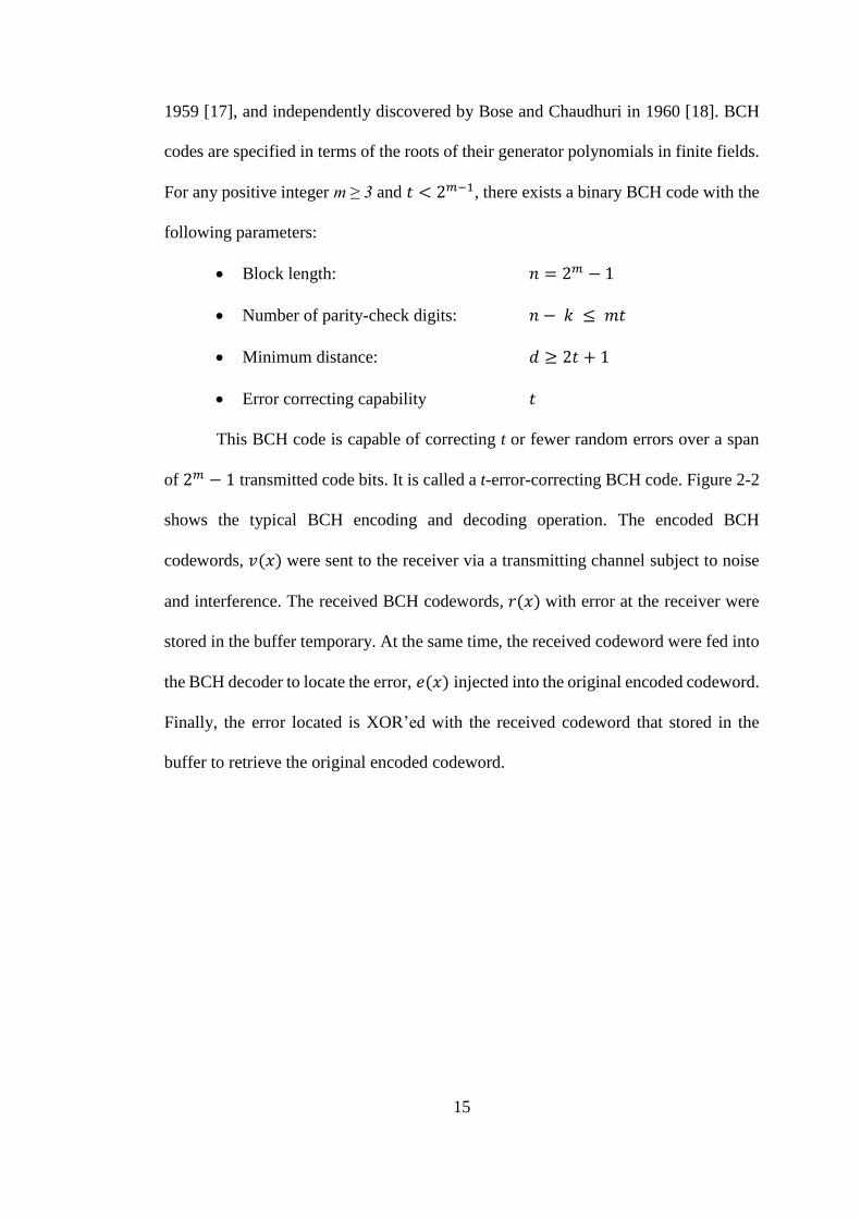
15
1959 [17], and independently discovered by Bose and Chaudhuri in 1960 [18]. BCH
codes are specified in terms of the roots of their generator polynomials in finite fields.
For any positive integer m ≥ 3 and 𝑡 < 2𝑚−1, there exists a binary BCH code with the
following parameters:
Block length: 𝑛 = 2𝑚 − 1
Number of parity-check digits: 𝑛 − 𝑘 ≤ 𝑚𝑡
Minimum distance: 𝑑 ≥ 2𝑡 + 1
Error correcting capability 𝑡
This BCH code is capable of correcting t or fewer random errors over a span
of 2𝑚 − 1 transmitted code bits. It is called a t-error-correcting BCH code. Figure 2-2
shows the typical BCH encoding and decoding operation. The encoded BCH
codewords, 𝑣(𝑥) were sent to the receiver via a transmitting channel subject to noise
and interference. The received BCH codewords, 𝑟(𝑥) with error at the receiver were
stored in the buffer temporary. At the same time, the received codeword were fed into
the BCH decoder to locate the error, 𝑒(𝑥) injected into the original encoded codeword.
Finally, the error located is XOR’ed with the received codeword that stored in the
buffer to retrieve the original encoded codeword.
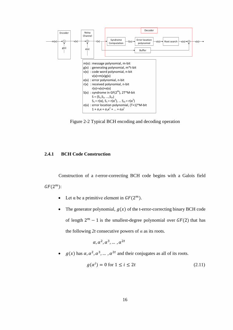
16
m(x) : message polynomial, m-bitg(x) : generating polynomial, m*t-bitv(x) : code word polynomial, n-bit
v(x)=m(x)g(x)e(x) : error polynomial, n-bitr(x) : received polynomial, n-bit
r(x)=v(x)+e(x)S(x) : syndrome in GF(2M), 2T*M-bit
S = (S1,S2, ...,S2t) S1 = r(α), S1 = r(α2), S2t = r(α2)
σ(x) : error location polynomial, (T+1)*M-bit 1 + σ1x + σ2x2 + + σtx
t
Syndrome Computation
Error location polynomial
Root searchS(x) σ(x)
Buffer
e(x) v(x)r(x)
Decoder
e(x)
Noisy Channel
m(x)
g(x)
v(x)
Encoder
Figure 2-2 Typical BCH encoding and decoding operation
2.4.1 BCH Code Construction
Construction of a t-error-correcting BCH code begins with a Galois field
𝐺𝐹(2𝑚):
Let α be a primitive element in 𝐺𝐹(2𝑚).
The generator polynomial, 𝑔(𝑥) of the t-error-correcting binary BCH code
of length 2𝑚 − 1 is the smallest-degree polynomial over 𝐺𝐹(2) that has
the following 2t consecutive powers of α as its roots.
𝛼, 𝛼2, 𝛼3, … , 𝛼2𝑡
𝑔(𝑥) has 𝛼, 𝛼2, 𝛼3, … , 𝛼2𝑡 and their conjugates as all of its roots.
𝑔(𝛼𝑖) = 0 for 1 ≤ 𝑖 ≤ 2𝑡 (2.11)
17
For 1 ≤ 𝑖 ≤ 2𝑡, let 𝜑𝑖(𝑥) be the minimal polynomial of 𝛼𝑖. Then 𝑔(𝑥) is
given by the least common multiple (LCM) of 𝜑1(𝑥), 𝜑2(𝑥), . . . , 𝜑2𝑡(𝑥),
that is:
𝑔(𝑥) = 𝐿𝐶𝑀{𝜑1(𝑥), 𝜑2(𝑥), . . . , 𝜑2𝑡(𝑥)} (2.12)
If i is an even integer, j is an odd integer and 𝑘 > 1, and i can be expressed
as 𝑖 = 𝑗2𝑘. Then 𝛼𝑖 = (𝛼𝑗) 2𝑙is a conjugate of 𝛼𝑗. Therefore,
𝜑𝑖(𝑥) = 𝜑𝑗(𝑥) (2.13)
Generator polynomial can be simplified as equation given by:
𝑔(𝑥) = 𝐿𝐶𝑀{𝜑1(𝑥), 𝜑3(𝑥), . . . , 𝜑2𝑡−1(𝑥)} (2.14)
The degree of 𝑔(𝑥) is at most mt, That is, the number of parity-checks digit,
𝑛 − 𝑘, of the code is at most equal to 𝑚𝑡.
2.4.2 Syndrome Calculation (SC)
Suppose a code polynomial 𝑣(𝑥) of a t-error-correcting BCH code, 𝑟(𝑥) be the
corresponding received polynomial and 𝑒(𝑥) be the error pattern:
The received polynomial is 𝑟(𝑥) given by:
𝑟(𝑥) = 𝑣(𝑥) + 𝑒(𝑥) (2.15)
The syndrome of 𝑟(𝑥) which consists of 2t syndrome components is given
by:
𝑆 = (𝑆1, 𝑆2, ⋯ , 𝑆2𝑡) = 𝑟 · 𝐻𝑇 (2.16)
For 1 ≤ 𝑖 ≤ 2𝑡, the 𝑖𝑡ℎ syndrome component is given by:
𝑆𝑖 = 𝑟(𝛼𝑖) = 𝑟0 + 𝑟1𝛼𝑖 + 𝑟2𝛼2𝑖, + ⋯ + 𝑟2𝑚−2𝛼(2𝑚−2)𝑖 (2.17)
18
Since 𝛼, 𝛼2, 𝛼3, … , 𝛼2𝑡 are roots of each code word polynomial, 𝑣(𝛼𝑖) =
0 for 1 ≤ 𝑖 ≤ 2𝑡 . From equation (2.15) and equation (2.17), the 𝑖𝑡ℎ
syndrome component can be expressed as equation (2.18)
𝑆𝑖 = 𝑒(𝛼𝑖) for 1 ≤ 𝑖 ≤ 2𝑡 (2.18)
If 𝑟(𝑥) is divided by the minimum polynomial 𝜑𝑖(𝑥) of 𝛼𝑖:
Since 𝜑𝑖(𝛼𝑖) = 0, then 𝑆𝑖 = 𝑟(𝛼𝑖) = 𝑏𝑖(𝛼𝑖) for 1 ≤ 𝑖 ≤ 2𝑡. We have:
𝑟(𝑥) = 𝑎𝑖(𝑥)𝜑𝑖(𝑥) + 𝑏𝑖(𝑥) (2.19)
where 𝑏𝑖(𝑥) is the remainder with degree less than that of 𝜑𝑖(𝑥).
2.4.3 Computation of Error Locator Polynomial
Suppose the error pattern, 𝑒(𝑥) contains ν errors at the locations 𝑗1, 𝑗2, ⋯ , 𝑗𝑣,
where 0 ≤ 𝑗1 < 𝑗2 < ⋯ < 𝑗𝑣 < 𝑛:
Then the error polynomial, 𝑒(𝑥) is given by:
𝑒(𝑥) = 𝑥𝑗1 + 𝑥𝑗2 + ⋯ + 𝑥𝑗𝑣 (2.20)
2t syndrome components, 𝑆1, 𝑆2, ⋯ , 𝑆2𝑡:
𝑆1 = 𝑒(𝛼) = 𝛼𝑗1 + 𝛼𝑗2 + ⋯ + 𝛼𝑗𝑣 ,
𝑆2 = 𝑒(𝛼2) = (𝛼𝑗1)2
+ (𝛼𝑗2)2
+ ⋯ + (𝛼𝑗𝑣)2,
⋮
𝑆2𝑡 = 𝑒(𝛼2𝑡) = (𝛼𝑗1)2𝑡
+ (𝛼𝑗2)2𝑡
+ ⋯ + (𝛼𝑗𝑣)2𝑡
(2.21)
For 1 ≤ 𝑙 ≤ 𝜈 , define 𝛽𝑙 = 𝛼𝑗𝑙 . 2t syndrome components can be
expressed in the similar form below:
𝑆1 = 𝛽1 + 𝛽2 + ⋯ + 𝛽𝑣,

19
𝑆2 = 𝛽12 + 𝛽2
2 + ⋯ + 𝛽𝑣2,
⋮
𝑆2𝑡 = 𝛽12𝑡 + 𝛽2
2𝑡 + ⋯ + 𝛽𝑣2𝑡
(2.22)
Define the error-location polynomial, 𝜎(𝑥) of degree ν over 𝐺𝐹(2𝑚) that
has 𝛽1−1, 𝛽2
−1, ⋯ , 𝛽𝑣−1
(the inverses of the location numbers 𝛽1, 𝛽2, ⋯ , 𝛽𝑣)
as roots:
𝜎(𝑥) = (1 + 𝛽1𝑥)(1 + 𝛽2𝑥) ⋯ (1 + 𝛽𝑣𝑥) = 𝜎0 + 𝜎1𝑥 + ⋯ + 𝜎𝑣𝑥𝑣 (2.23)
where,
𝜎0 = 1,
𝜎1 = 𝛽1 + 𝛽2 + ⋯ + 𝛽𝑣,
𝜎2 = 𝛽1𝛽2 + 𝛽1𝛽3 + ⋯ + 𝛽𝑣−1𝛽𝑣,
𝜎3 = 𝛽1𝛽2𝛽3 + 𝛽1𝛽2𝛽4 + ⋯ + 𝛽𝑣−2𝛽𝑣−1𝛽𝑣
⋮
𝜎𝑣 = 𝛽1𝛽2𝛽3 ⋯ 𝛽𝑣−2𝛽𝑣−1𝛽𝑣.
The inverses of the roots of error-location polynomial, 𝜎(𝑥) give the error-
location numbers.
From equation (2.21) and equation (2.22), 2t syndrome components,
𝑆1, 𝑆2, ⋯ , 𝑆2𝑡 can be expressed in terms of the coefficients of the error-
location polynomial, 𝜎0, 𝜎1, ⋯ , 𝜎𝑣:
𝑆1 + 𝜎1 = 0,
𝑆2 + 𝜎1𝑆1 + 2𝜎2 = 0,
𝑆3 + 𝜎1𝑆2 + 𝜎2𝑆1 + 3𝜎3 = 0,
⋮
𝑆𝑣 + 𝜎1𝑆𝑣−1 + 𝜎2𝑆𝑣−2 + ⋯ 𝜎𝑣−1𝑆1 + 𝑣𝜎𝑣 = 0,
20
𝑆𝑣+1 + 𝜎1𝑆𝑣 + 𝜎2𝑆𝑣−1 + ⋯ 𝜎𝑣−1𝑆2 + 𝜎𝑣𝑆1 = 0, (2.24)
Above identities is called Newton identities.
In general there will be more than one error pattern for which the coefficients
of its error-location polynomial satisfy the Newton identities. To minimize the
probability of a decoding error, the most probable error pattern for error correction
need to be found. Finding the most probable error pattern means determining the error-
location polynomial of minimum degree whose coefficients satisfy the Newton
identities. This can be achieved iteratively by Berlekamp–Massey (BM) algorithm.
2.4.4 Berlekamp-Massey Algorithm (BMA)
Berlekamp-Massey algorithm [19] [20] is an algorithm that will be used in
BCH decoder to find the error-location polynomial, 𝜎(𝑥) iteratively in 2t steps:
For 1 ≤ 𝑘 ≤ 2𝑡, the algorithm at the k-th step gives an error-location
polynomial of minimum degree as below:
𝜎(𝑘)(𝑥) = 𝜎0(𝑘) + 𝜎1
(𝑘)𝑥 + ⋯ + 𝜎𝑙𝑘
(𝑘)𝑥𝑙𝑘 (2.25)
where coefficients satisfy the first k Newton identities.
(k+1)th step error-location polynomial, 𝜎(𝑘+1)(𝑥) is given by:
𝜎(𝑘+1)(𝑥) = 𝜎(𝑘)(𝑥) + 𝑑𝑘𝑑𝑖−1𝑥𝑘−𝑖𝜎(𝑖)(𝑥) (2.26)
where
𝑑𝑘𝑑𝑖−1𝑥𝑘−𝑖𝜎(𝑖)(𝑥) is the correction term
𝑑𝑘 is the kth discrepancy 𝑑𝑘 = 𝑆𝑘+1 +
𝜎1(𝑘)𝑆𝑘 + 𝜎2
(𝑘)𝑆𝑘−1 + ⋯ + 𝜎𝑙𝑘
(𝑘)𝑆𝑘+1−𝑙𝑘

21
𝑑𝑖−1
is inverse of ith discrepancy
𝑖 is the step prior to k which is 𝜎(𝑖)(𝑥) such that
the ith discrepancy, 𝑑𝑖 ≠ 0 and 𝑖 − 𝑙𝑖 has the largest value.
𝑙𝑖 is the degree of 𝜎(𝑖)(𝑥)
Steps of using BM algorithm for finding the Error-Location Polynomial of
a BCH Code:
o Initialization:
For 𝑘 = −1, set 𝜎(−1)(𝑋) = 1, 𝑑−1 = 1, 𝑙−1 = 0 and −1 −
𝑙−1 = −1.
For 𝑘 = 0, set 𝜎(0)(𝑋) = 1, 𝑑0 = 𝑆1, 𝑙0 = 0 and 0 − 𝑙0 = 0.
o Step 1: If 𝑘 = 2𝑡 , output 𝜎(𝑘)(𝑋) as the error-location polynomial
𝜎(𝑥); otherwise go to Step 2.
o Step 2: Compute 𝑑𝑘 and go to Step 3.
o Step 3: If 𝑑𝑘 = 0 , set 𝜎(𝑘+1)(𝑋) = 𝜎(𝑘)(𝑋) ; otherwise, set
𝜎(𝑘+1)(𝑋) = 𝜎(𝑘)(𝑋) + 𝑑𝑘𝑑𝑖−1𝑥𝑘−𝑖𝜎(𝑖)(𝑋). Go to Step 4.
o Step 4: 𝑘 ← 𝑘 + 1. Go to Step 1.
The BM algorithm can be executed by setting up and filling in the
following table 2.4:

22
Table 2-4 BMA execution table
Step
k
Partial solution
𝜎(𝑘)(𝑋)
Discrepancy
𝑑𝑘
Degree
𝑙𝑘
Step/degree difference
𝑘 − 𝑙𝑘
-1 1 1 0 – 1
0 1 𝑆1 0 0
1 𝜎(1)(𝑋) 𝑑1 𝑙1 1 − 𝑙1
2 𝜎(2)(𝑋) 𝑑2 𝑙2 2 − 𝑙2
⋮
2t 𝜎(2𝑡)(𝑋) ----- ----- -----
Based on the above BM algorithm, an interesting pattern k-th step solution will
be observed. The solution 𝜎(2𝑘−1)(𝑥) at the (2k−1)th step of the BMA is also the
solution 𝜎(2𝑘)(𝑥) at the 2k-th step of the BMA:
𝜎(2𝑘)(𝑥) = 𝜎(2𝑘−1)(𝑥), for 1 ≤ 𝑘 ≤ 𝑡 (2.27)
Consequently, for decoding a binary BCH code, the BM algorithm can be
simplified as follows:
Steps of using Simplified BM algorithm for finding the Error-Location
Polynomial of a BCH Code:
o Initialization:
For 𝑘 = − 12⁄ , set 𝜎(−1
2⁄ )(𝑋) = 1, 𝑑−12⁄ = 1, 𝑙−1
2⁄ = 0 and
−2(12⁄ ) − 𝑙−1
2⁄ = −1.
For 𝑘 = 0, set 𝜎(0)(𝑋) = 1, 𝑑0 = 𝑆1, 𝑙0 = 0 and 0 − 𝑙0 = 0.
o Step 1: If 𝑘 = 𝑡, output 𝜎(𝑘)(𝑋) as the error-location polynomial 𝜎(𝑥);
otherwise go to Step 2.
o Step 2: Compute 𝑑𝑘 = 𝑆2𝑘+1 + 𝜎1(𝑘)𝑆2𝑘 + 𝜎2
(𝑘)𝑆2𝑘−1 + ⋯ +
𝜎𝑙𝑘
(𝑘)𝑆2𝑘+1−𝑙𝑘 and go to Step 3.

23
o Step 3: If 𝑑𝑘 = 0 , set 𝜎(𝑘+1)(𝑋) = 𝜎(𝑘)(𝑋) ; otherwise, set
𝜎(𝑘+1)(𝑋) = 𝜎(𝑘)(𝑋) + 𝑑𝑘𝑑𝑖−1𝑋2(𝑘−𝑖)𝜎(𝑖)(𝑋). Go to Step 4.
o Step 4: 𝑘 ← 𝑘 + 1. Go to Step 1.
The simplified BM algorithm can be executed by setting up and filling in
the following table 2-5:
Table 2-5 Simplified BMA execution table
Step
k
Partial solution
𝜎(𝑘)(𝑋)
Discrepancy
𝑑𝑘
Degree
𝑙𝑘
Step/degree difference
2𝑘 − 𝑙𝑘
– ½ 1 1 0 – 1
0 1 𝑆1 0 0
1 𝜎(1)(𝑋) 𝑑1 𝑙1 2 − 𝑙1
2 𝜎(2)(𝑋) 𝑑2 𝑙2 4 − 𝑙2
⋮
t 𝜎(𝑡)(𝑋) ----- ----- -----
It can be noticed that from either the conventional or simplified BMA, the
evaluation of the correction term in each iteration required GF inverter. However,
designing a GF inverter and running it at each iteration consume extra logic and impose
additional delay in the calculation. Therefore, the inversion-less BMA [21] was
introduced and several improvements [11] [14] [15] were proposed by researchers to
eliminate the GF inverter that relax the complexity of the BMA design.
24
2.4.5 Chien Search (CS)
After the error location polynomial is obtained, the error locations are found
by finding the all the roots from the error location polynomial. The error location is
the power of alpha from each of the roots found.
Consider error location polynomial, 𝜎(𝑥) in equation (2.28).
𝜎(𝑥) = 𝜎0 + 𝜎1𝑥 + 𝜎2𝑥2 + ⋯ + 𝜎𝑣𝑥𝑣 (2.28)
One method to find the roots is evaluating 𝜎(𝑥) with each non-zero element in
𝐺𝐹(2𝑚) , (1, 𝛼, 𝛼2, 𝛼3, … , 𝛼2𝑚−2) . However, this will require a lot of variable
multiplication and addition.
The Chien Search algorithm observed that:
Let 𝜆𝑗,𝑖 = 𝜎𝑗(𝛼𝑖)𝑗, then
𝜎(𝛼𝑖) = 𝜎0 + 𝜎1𝛼𝑖 + 𝜎2(𝛼𝑖)2
+ ⋯ + 𝜎𝑣(𝛼𝑖)𝑡 (2.29)
𝜎(𝛼𝑖) = 𝜆0,𝑖 + 𝜆1,𝑖 + 𝜆2,𝑖 + ⋯ + 𝜆𝑡,𝑖 (2.30)
𝜎(𝛼𝑖+1) = 𝜎0 + 𝜎1𝛼𝑖+1 + 𝜎2(𝛼𝑖+1)2
+ ⋯ + 𝜎𝑣(𝛼𝑖+1)𝑡 (2.31)
𝜎(𝛼𝑖+1) = 𝜎0 + 𝜎1(𝛼𝑖)𝛼1 + 𝜎2(𝛼𝑖)2
𝛼2 + ⋯ + 𝜎𝑣(𝛼𝑖)𝑡𝛼𝑡 (2.32)
𝜎(𝛼𝑖+1) = 𝜆0,𝑖 + 𝜆1,𝑖𝛼1 + 𝜆2,𝑖𝛼
2 + ⋯ + 𝜆𝑡,𝑖𝛼𝑡 (2.33)
From equation (2.29), (2.30), (2.31), (2.32) and (2.33), it can be observed
that:
𝜆𝑗,𝑖+1 = 𝜆𝑗,𝑖𝛼𝑗 (2.34)
If ∑ 𝜆𝑗,𝑖𝑡𝑗=0 = 0, then 𝛼𝑖 is a root. For each of the 𝛼𝑖, 𝑖 will be the bit location
of the received codeword that contains error.