Approved for public release. Distribution is unlimited.

ARES I-X RANGE SAFETY FLIGHT ENVELOPE ANALYSIS

B.R. Starr NASA Langley Research Center

Hampton, VA

A.D. Olds Analytical Mechanics Associates, Inc.

Hampton, VA

A.S. Craig

Jacobs Engineering Huntsville, AL

ABSTRACT

Ares I-X was the first test flight of the Ares I Crew Launch Vehicle. The Ares I-X Flight Test Vehicle was successfully launched from Kennedy Space Center’s launch complex 39 pad B on October 28th, 2009. Prior to flight, the U. S. Air Force 45th Space Wing required the test program to develop flight envelopes that defined the limits of normal operation as part of a flight data package required to obtain flight approval. This paper documents the flight envelope requirements, the analysis conducted to meet those requirements, and a comparison of the analysis results to the Ares I-X best estimated trajectory developed from flight data, as a means of assessing the pre-flight envelopes’ adequacy in encompassing the actual flight. Probabilistic analyses of the Ares I-X ascent profile were conducted to develop six flight envelopes of the vehicle trajectory in the Range Safety vertical and horizontal planes. Due to variability in the launch schedule, seasonal envelopes were developed to encompass launch environments from July through November. Monte Carlo analyses were conducted to determine the effects of vehicle system uncertainty in the presence of each of the worst case wind profiles. The analyses included uncertainty models for atmospheric properties, aerodynamics, mass properties, engine performance, and guidance and actuator performance. The resulting dispersed trajectories were statistically analyzed to determine the envelopes for a launch season from July to November. Comparisons to the Flight Test Vehicle best estimated trajectory showed the flight was nominal and was within all six envelopes.

INTRODUCTION

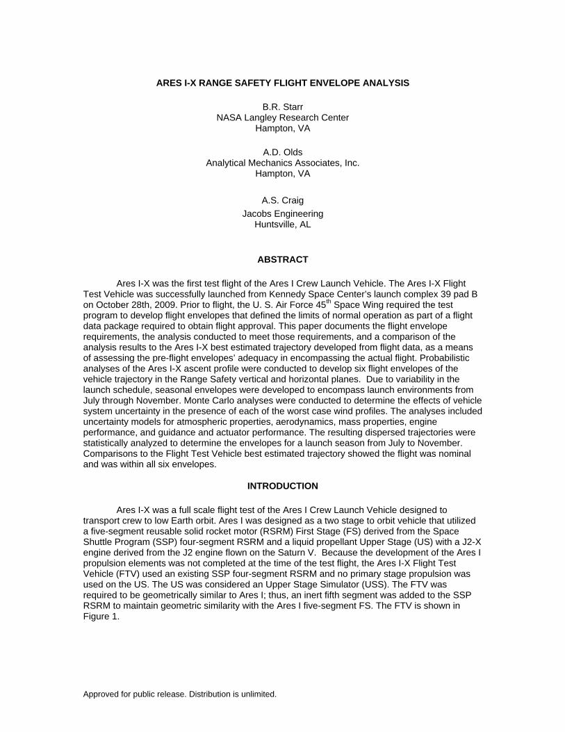
Ares I-X was a full scale flight test of the Ares I Crew Launch Vehicle designed to transport crew to low Earth orbit. Ares I was designed as a two stage to orbit vehicle that utilized a five-segment reusable solid rocket motor (RSRM) First Stage (FS) derived from the Space Shuttle Program (SSP) four-segment RSRM and a liquid propellant Upper Stage (US) with a J2-X engine derived from the J2 engine flown on the Saturn V. Because the development of the Ares I propulsion elements was not completed at the time of the test flight, the Ares I-X Flight Test Vehicle (FTV) used an existing SSP four-segment RSRM and no primary stage propulsion was used on the US. The US was considered an Upper Stage Simulator (USS). The FTV was required to be geometrically similar to Ares I; thus, an inert fifth segment was added to the SSP RSRM to maintain geometric similarity with the Ares I five-segment FS. The FTV is shown in Figure 1.

2

Figure 1 Ares I-X Flight Test Vehicle

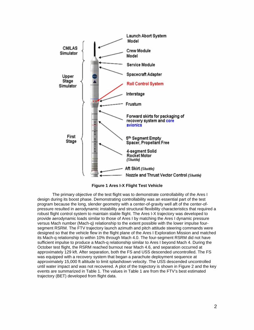
The primary objective of the test flight was to demonstrate controllability of the Ares I design during its boost phase. Demonstrating controllability was an essential part of the test program because the long, slender geometry with a center-of-gravity well aft of the center-of-pressure resulted in aerodynamic instability and structural flexibility characteristics that required a robust flight control system to maintain stable flight. The Ares I-X trajectory was developed to provide aerodynamic loads similar to those of Ares I by matching the Ares I dynamic pressure versus Mach number (Mach-q) relationship to the extent possible with the lower impulse four-segment RSRM. The FTV trajectory launch azimuth and pitch attitude steering commands were designed so that the vehicle flew in the flight plane of the Ares I Exploration Mission and matched its Mach-q relationship to within 10% through Mach 4.0. The four-segment RSRM did not have sufficient impulse to produce a Mach-q relationship similar to Ares I beyond Mach 4. During the October test flight, the RSRM reached burnout near Mach 4.6, and separation occurred at approximately 129 kft. After separation, both the FS and USS descended uncontrolled. The FS was equipped with a recovery system that began a parachute deployment sequence at approximately 15,000 ft altitude to limit splashdown velocity. The USS descended uncontrolled until water impact and was not recovered. A plot of the trajectory is shown in Figure 2 and the key events are summarized in Table 1. The values in Table 1 are from the FTV’s best estimated trajectory (BET) developed from flight data.

3

Figure 2 Ares I-X Test Flight Trajectory

Table 1 Ares I-X Test Flight Trajectory Events

Event Time (s) Downrange (nmi) Altitude (kft) q (psf)

Ascent max q 58 3.8 38.9 874

Separation 123 36.4 128.6 102

USS apogee 159 63.9 148.9 37

FS apogee 160 63.9 149.1 35

USS reentry max q 249 122.6 42.7 2355

FS reentry max q 254 119.1 51.8 1060

USS water impact 310 130.8 0 503

FS water impact 352 122.1 0 13

The test flight was launched from Kennedy Space Center (KSC) Launch Complex 39, Pad B and flew on the Eastern Range. Because the test flight was conducted on the Eastern Range, the Ares I-X Test Program was required to obtain flight plan approval from the United States Air Force’s 45th Space Wing (45SW) and was subject to flight safety requirements documented in Reference 1. Range Safety (RS) analyses were conducted to meet the flight safety requirements specified in the Air Force Space Command Manual (AFSPCMAN) 91-710, Volume 2. The analyses data products were submitted to the 45SW in a flight data package to support the request for flight plan approval. The 45SW used the data packages to determine the risk of casualty to the public posed by the flight, to develop flight displays for monitoring the FTV

4

during its powered flight, and to develop flight rules regarding what action to take in the event of an anomaly.

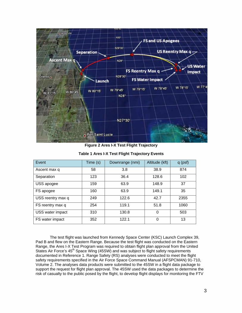
Flight envelopes that define the limits of normal flight are one data product required by AFSPCMAN 91-710. The flight envelopes define the limits of a normally operating vehicle in the Range Safety horizontal and vertical planes by encompassing three sigma dispersed trajectories for each month in the launch season. A total of six flight envelopes are required to define the limits of normal operation, four horizontal plane envelopes and two vertical plane envelopes. The horizontal plane is a plan view of the trajectory in which the downrange position and latitude of the FTV’s vacuum instantaneous impact point (IIP) is monitored. The four horizontal plane envelopes consist of the maximum instantaneous impact point (MaxIIP), the minimum instantaneous impact point (MinIIP), the left instantaneous impact point (LIIP), and the right instantaneous impact point (RIIP) envelopes. The MaxIIP and MinIIP envelopes define the maximum and minimum IIP downrange position of a normally operating FTV as a function of time. The LIIP and RIIP envelopes define the maximum left and right IIP latitude of a normally operating FTV as a function of longitude. Figure 3 shows an illustration of the horizontal plane with notional LIIP and RIIP envelopes and an example of the MaxIIP and MinIIP at a given time in flight.

Figure 3 Range Safety Horizontal Plane LIIP and RIIP Flight Envelopes

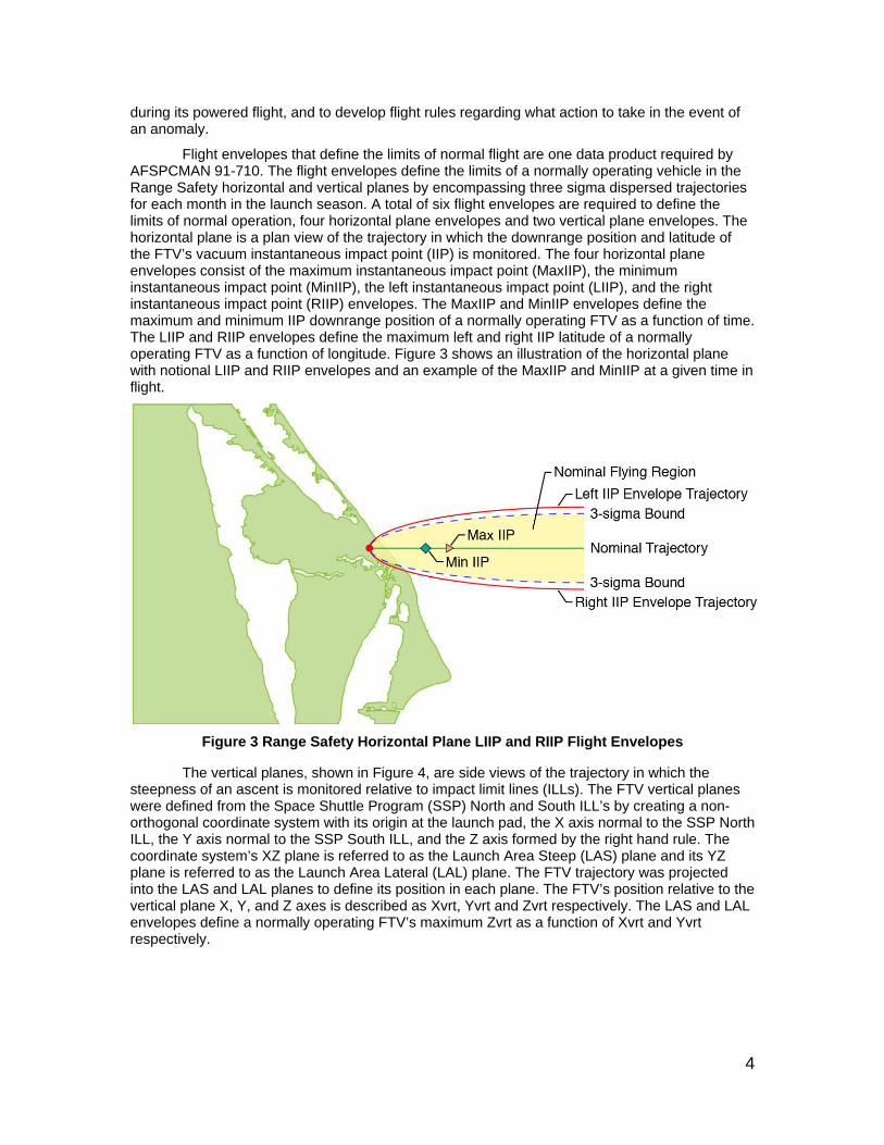
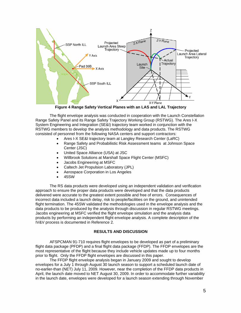
The vertical planes, shown in Figure 4, are side views of the trajectory in which the steepness of an ascent is monitored relative to impact limit lines (ILLs). The FTV vertical planes were defined from the Space Shuttle Program (SSP) North and South ILL’s by creating a non-orthogonal coordinate system with its origin at the launch pad, the X axis normal to the SSP North ILL, the Y axis normal to the SSP South ILL, and the Z axis formed by the right hand rule. The coordinate system’s XZ plane is referred to as the Launch Area Steep (LAS) plane and its YZ plane is referred to as the Launch Area Lateral (LAL) plane. The FTV trajectory was projected into the LAS and LAL planes to define its position in each plane. The FTV’s position relative to the vertical plane X, Y, and Z axes is described as Xvrt, Yvrt and Zvrt respectively. The LAS and LAL envelopes define a normally operating FTV’s maximum Zvrt as a function of Xvrt and Yvrt respectively.

5

Figure 4 Range Safety Vertical Planes with an LAS and LAL Trajectory

The flight envelope analysis was conducted in cooperation with the Launch Constellation Range Safety Panel and its Range Safety Trajectory Working Group (RSTWG). The Ares I-X System Engineering and Integration (SE&I) trajectory team worked in conjunction with the RSTWG members to develop the analysis methodology and data products. The RSTWG consisted of personnel from the following NASA centers and support contractors:

Ares I-X SE&I trajectory team at Langley Research Center (LaRC) Range Safety and Probabilistic Risk Assessment teams at Johnson Space

Center (JSC) United Space Alliance (USA) at JSC Willbrook Solutions at Marshall Space Flight Center (MSFC) Jacobs Engineering at MSFC Caltech Jet Propulsion Laboratory (JPL) Aerospace Corporation in Los Angeles 45SW

The RS data products were developed using an independent validation and verification

approach to ensure the proper data products were developed and that the data products delivered were accurate to the greatest extent possible and free of errors. Consequences of incorrect data included a launch delay, risk to people/facilities on the ground, and unintended flight termination. The 45SW validated the methodologies used in the envelope analysis and the data products to be produced by the analysis through discussion in regular RSTWG meetings. Jacobs engineering at MSFC verified the flight envelope simulation and the analysis data products by performing an independent flight envelope analysis. A complete description of the IV&V process is documented in Reference 2.

RESULTS AND DISCUSSION

AFSPCMAN 91-710 requires flight envelopes to be developed as part of a preliminary flight data package (PFDP) and a final flight data package (FFDP). The FFDP envelopes are the most representative of the flight because they include vehicle updates made up to four months prior to flight. Only the FFDP flight envelopes are discussed in this paper.

The FFDP flight envelope analysis began in January 2009 and sought to develop envelopes for a July 1 through August 30 launch season to support a scheduled launch date of no-earlier-than (NET) July 11, 2009. However, near the completion of the FFDP data products in April, the launch date moved to NET August 30, 2009. In order to accommodate further variability in the launch date, envelopes were developed for a launch season extending through November

6

30, 2009. The flight envelopes were required to encompass 3-sigma dispersions in the horizontal and vertical planes expected about the nominal trajectory for each month in the launch season. Hence, the envelope analysis began with the development of monthly nominal trajectories.

Development of the nominal trajectories was a two-step process that involved the use of a 3-DOF and a 6-DOF simulation. First, a 3-DOF optimization simulation was used to develop steering commands that provided the best possible match of the Ares I Mach-q profile for each month in the launch season. The 3-DOF simulation minimized the difference between the FTV and Ares I Mach-q relationships by optimizing the FTV’s pitch attitude steering commands for each month’s mean monthly atmosphere, winds, and RSRM propellant mean bulk temperature (PMBT). Refer to Reference 3 for a complete description of the optimization simulation. Monthly steering tables that defined the FTV pitch attitude as a function of altitude were created from the Mach-q optimized trajectories. Next, the steering tables, referred to as Chi tables, were used as the input to the FFDP 6-DOF trajectory simulation’s guidance algorithm to define the monthly nominal trajectories. Both the 3-DOF optimization and the 6-DOF FFDP simulations were developed in the Program to Optimize Simulated Trajectories II (POST II) software4.

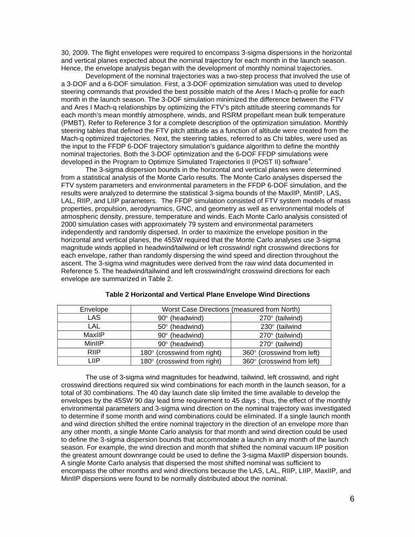
The 3-sigma dispersion bounds in the horizontal and vertical planes were determined from a statistical analysis of the Monte Carlo results. The Monte Carlo analyses dispersed the FTV system parameters and environmental parameters in the FFDP 6-DOF simulation, and the results were analyzed to determine the statistical 3-sigma bounds of the MaxIIP, MinIIP, LAS, LAL, RIIP, and LIIP parameters. The FFDP simulation consisted of FTV system models of mass properties, propulsion, aerodynamics, GNC, and geometry as well as environmental models of atmospheric density, pressure, temperature and winds. Each Monte Carlo analysis consisted of 2000 simulation cases with approximately 79 system and environmental parameters independently and randomly dispersed. In order to maximize the envelope position in the horizontal and vertical planes, the 45SW required that the Monte Carlo analyses use 3-sigma magnitude winds applied in headwind/tailwind or left crosswind/ right crosswind directions for each envelope, rather than randomly dispersing the wind speed and direction throughout the ascent. The 3-sigma wind magnitudes were derived from the raw wind data documented in Reference 5. The headwind/tailwind and left crosswind/right crosswind directions for each envelope are summarized in Table 2.

Table 2 Horizontal and Vertical Plane Envelope Wind Directions

Envelope Worst Case Directions (measured from North) LAS 90 (headwind) 270 (tailwind) LAL 50 (headwind) 230 (tailwind

MaxIIP 90 (headwind) 270 (tailwind) MinIIP 90 (headwind) 270 (tailwind) RIIP 180 (crosswind from right) 360 (crosswind from left) LIIP 180 (crosswind from right) 360 (crosswind from left)

The use of 3-sigma wind magnitudes for headwind, tailwind, left crosswind, and right

crosswind directions required six wind combinations for each month in the launch season, for a total of 30 combinations. The 40 day launch date slip limited the time available to develop the envelopes by the 45SW 90 day lead time requirement to 45 days ; thus, the effect of the monthly environmental parameters and 3-sigma wind direction on the nominal trajectory was investigated to determine if some month and wind combinations could be eliminated. If a single launch month and wind direction shifted the entire nominal trajectory in the direction of an envelope more than any other month, a single Monte Carlo analysis for that month and wind direction could be used to define the 3-sigma dispersion bounds that accommodate a launch in any month of the launch season. For example, the wind direction and month that shifted the nominal vacuum IIP position the greatest amount downrange could be used to define the 3-sigma MaxIIP dispersion bounds. A single Monte Carlo analysis that dispersed the most shifted nominal was sufficient to encompass the other months and wind directions because the LAS, LAL, RIIP, LIIP, MaxIIP, and MinIIP dispersions were found to be normally distributed about the nominal.

7

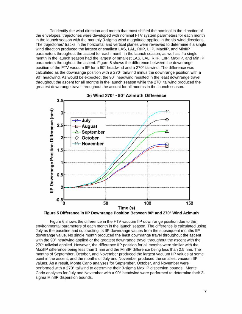
To identify the wind direction and month that most shifted the nominal in the direction of the envelopes, trajectories were developed with nominal FTV system parameters for each month in the launch season with the monthly 3-sigma wind magnitude applied in the six wind directions. The trajectories’ tracks in the horizontal and vertical planes were reviewed to determine if a single wind direction produced the largest or smallest LAS, LAL, RIIP, LIIP, MaxIIP, and MinIIP parameters throughout the ascent for each month in the launch season, as well as if a single month in the launch season had the largest or smallest LAS, LAL, RIIP, LIIP, MaxIIP, and MinIIP parameters throughout the ascent. Figure 5 shows the difference between the downrange position of the FTV vacuum IIP for a 90 headwind and a 270 tailwind. The difference was calculated as the downrange position with a 270 tailwind minus the downrange position with a 90 headwind. As would be expected, the 90 headwind resulted in the least downrange travel throughout the ascent for all months in the launch season while the 270 tailwind produced the greatest downrange travel throughout the ascent for all months in the launch season.

Figure 5 Difference in IIP Downrange Position Between 90 and 270 Wind Azimuth

Figure 6 shows the difference in the FTV vacuum IIP downrange position due to the environmental parameters of each month in the launch season. The difference is calculated using July as the baseline and subtracting its IIP downrange values from the subsequent months IIP downrange value. No single month produced the least downrange travel throughout the ascent with the 90 headwind applied or the greatest downrange travel throughout the ascent with the 270 tailwind applied. However, the difference IIP position for all months were similar with the MaxIIP difference being less than 1 nmi and the MinIIP difference being less than 2.5 nmi. The months of September, October, and November produced the largest vacuum IIP values at some point in the ascent, and the months of July and November produced the smallest vacuum IIP values. As a result, Monte Carlo analyses for September, October, and November were performed with a 270 tailwind to determine their 3-sigma MaxIIP dispersion bounds. Monte Carlo analyses for July and November with a 90 headwind were performed to determine their 3-sigma MinIIP dispersion bounds.

8

Figure 6 Difference in IIP Downrange Position Due to Launch Month

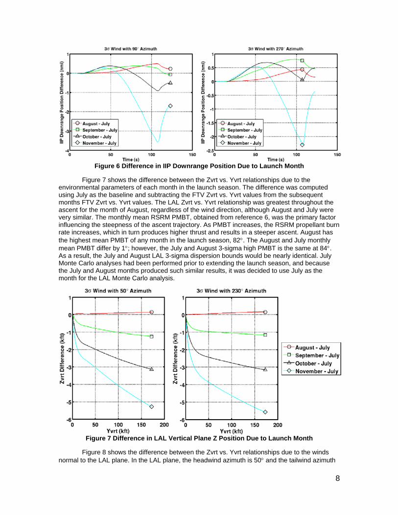
Figure 7 shows the difference between the Zvrt vs. Yvrt relationships due to the environmental parameters of each month in the launch season. The difference was computed using July as the baseline and subtracting the FTV Zvrt vs. Yvrt values from the subsequent months FTV Zvrt vs. Yvrt values. The LAL Zvrt vs. Yvrt relationship was greatest throughout the ascent for the month of August, regardless of the wind direction, although August and July were very similar. The monthly mean RSRM PMBT, obtained from reference 6, was the primary factor influencing the steepness of the ascent trajectory. As PMBT increases, the RSRM propellant burn rate increases, which in turn produces higher thrust and results in a steeper ascent. August has the highest mean PMBT of any month in the launch season, 82. The August and July monthly mean PMBT differ by 1; however, the July and August 3-sigma high PMBT is the same at 84. As a result, the July and August LAL 3-sigma dispersion bounds would be nearly identical. July Monte Carlo analyses had been performed prior to extending the launch season, and because the July and August months produced such similar results, it was decided to use July as the month for the LAL Monte Carlo analysis.

Figure 7 Difference in LAL Vertical Plane Z Position Due to Launch Month

Figure 8 shows the difference between the Zvrt vs. Yvrt relationships due to the winds normal to the LAL plane. In the LAL plane, the headwind azimuth is 50 and the tailwind azimuth

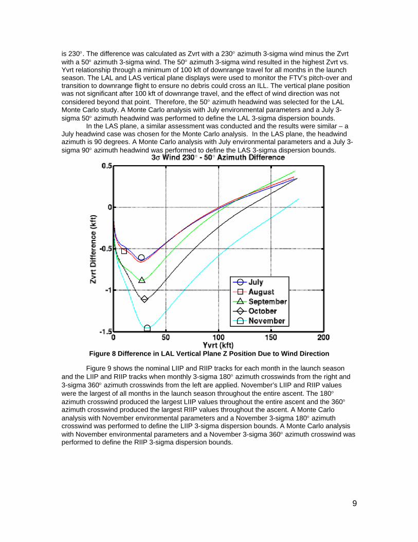
9

is 230. The difference was calculated as Zvrt with a 230 azimuth 3-sigma wind minus the Zvrt with a 50 azimuth 3-sigma wind. The 50 azimuth 3-sigma wind resulted in the highest Zvrt vs. Yvrt relationship through a minimum of 100 kft of downrange travel for all months in the launch season. The LAL and LAS vertical plane displays were used to monitor the FTV’s pitch-over and transition to downrange flight to ensure no debris could cross an ILL. The vertical plane position was not significant after 100 kft of downrange travel, and the effect of wind direction was not considered beyond that point. Therefore, the 50 azimuth headwind was selected for the LAL Monte Carlo study. A Monte Carlo analysis with July environmental parameters and a July 3-sigma 50 azimuth headwind was performed to define the LAL 3-sigma dispersion bounds.

In the LAS plane, a similar assessment was conducted and the results were similar – a July headwind case was chosen for the Monte Carlo analysis. In the LAS plane, the headwind azimuth is 90 degrees. A Monte Carlo analysis with July environmental parameters and a July 3-sigma 90 azimuth headwind was performed to define the LAS 3-sigma dispersion bounds.

Figure 8 Difference in LAL Vertical Plane Z Position Due to Wind Direction

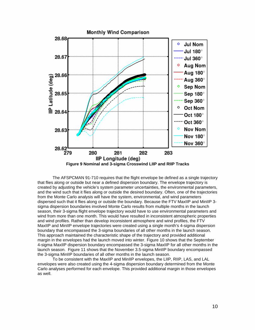
Figure 9 shows the nominal LIIP and RIIP tracks for each month in the launch season and the LIIP and RIIP tracks when monthly 3-sigma 180 azimuth crosswinds from the right and 3-sigma 360 azimuth crosswinds from the left are applied. November’s LIIP and RIIP values were the largest of all months in the launch season throughout the entire ascent. The 180 azimuth crosswind produced the largest LIIP values throughout the entire ascent and the 360 azimuth crosswind produced the largest RIIP values throughout the ascent. A Monte Carlo analysis with November environmental parameters and a November 3-sigma 180 azimuth crosswind was performed to define the LIIP 3-sigma dispersion bounds. A Monte Carlo analysis with November environmental parameters and a November 3-sigma 360 azimuth crosswind was performed to define the RIIP 3-sigma dispersion bounds.

10

Figure 9 Nominal and 3-sigma Crosswind LIIP and RIIP Tracks

The AFSPCMAN 91-710 requires that the flight envelope be defined as a single trajectory

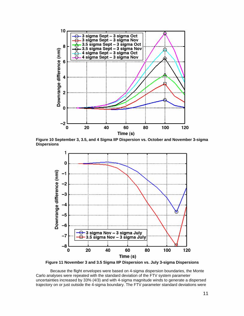
that flies along or outside but near a defined dispersion boundary. The envelope trajectory is created by adjusting the vehicle’s system parameter uncertainties, the environmental parameters, and the wind such that it flies along or outside the desired boundary. Often, one of the trajectories from the Monte Carlo analysis will have the system, environmental, and wind parameters dispersed such that it flies along or outside the boundary. Because the FTV MaxIIP and MinIIP 3-sigma dispersion boundaries involved Monte Carlo results from multiple months in the launch season, their 3-sigma flight envelope trajectory would have to use environmental parameters and wind from more than one month. This would have resulted in inconsistent atmospheric properties and wind profiles. Rather than develop inconsistent atmosphere and wind profiles, the FTV MaxIIP and MinIIP envelope trajectories were created using a single month’s 4-sigma dispersion boundary that encompassed the 3-sigma boundaries of all other months in the launch season. This approach maintained the characteristic shape of the trajectory and provided additional margin in the envelopes had the launch moved into winter. Figure 10 shows that the September 4-sigma MaxIIP dispersion boundary encompassed the 3-sigma MaxIIP for all other months in the launch season. Figure 11 shows that the November 3.5-sigma MinIIP boundary encompassed the 3-sigma MinIIP boundaries of all other months in the launch season.

To be consistent with the MaxIIP and MinIIP envelopes, the LIIP, RIIP, LAS, and LAL envelopes were also created using the 4-sigma dispersion boundary determined from the Monte Carlo analyses performed for each envelope. This provided additional margin in those envelopes as well.

11

Figure 10 September 3, 3.5, and 4 Sigma IIP Dispersion vs. October and November 3-sigma Dispersions

Figure 11 November 3 and 3.5 Sigma IIP Dispersion vs. July 3-sigma Dispersions

Because the flight envelopes were based on 4-sigma dispersion boundaries, the Monte Carlo analyses were repeated with the standard deviation of the FTV system parameter uncertainties increased by 33% (4/3) and with 4-sigma magnitude winds to generate a dispersed trajectory on or just outside the 4-sigma boundary. The FTV parameter standard deviations were

12

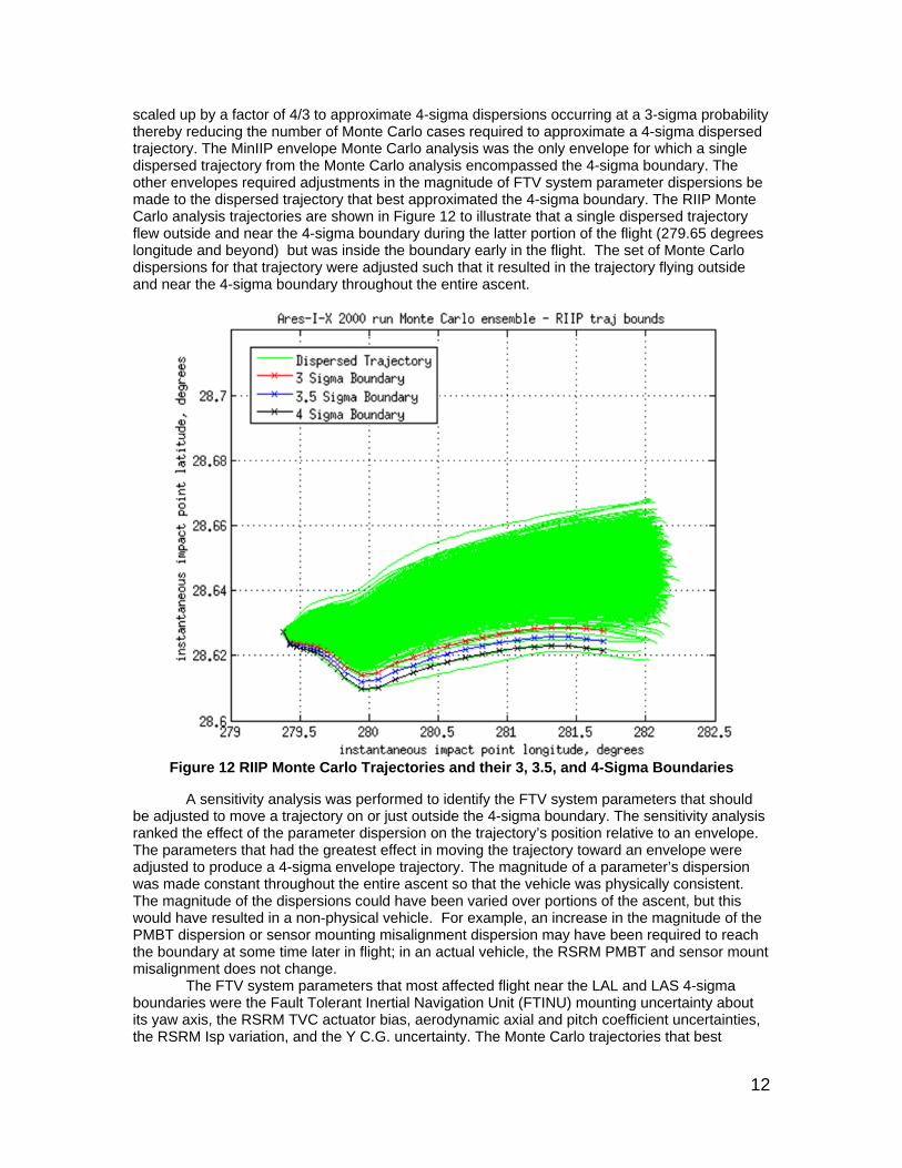
scaled up by a factor of 4/3 to approximate 4-sigma dispersions occurring at a 3-sigma probability thereby reducing the number of Monte Carlo cases required to approximate a 4-sigma dispersed trajectory. The MinIIP envelope Monte Carlo analysis was the only envelope for which a single dispersed trajectory from the Monte Carlo analysis encompassed the 4-sigma boundary. The other envelopes required adjustments in the magnitude of FTV system parameter dispersions be made to the dispersed trajectory that best approximated the 4-sigma boundary. The RIIP Monte Carlo analysis trajectories are shown in Figure 12 to illustrate that a single dispersed trajectory flew outside and near the 4-sigma boundary during the latter portion of the flight (279.65 degrees longitude and beyond) but was inside the boundary early in the flight. The set of Monte Carlo dispersions for that trajectory were adjusted such that it resulted in the trajectory flying outside and near the 4-sigma boundary throughout the entire ascent.

Figure 12 RIIP Monte Carlo Trajectories and their 3, 3.5, and 4-Sigma Boundaries

A sensitivity analysis was performed to identify the FTV system parameters that should be adjusted to move a trajectory on or just outside the 4-sigma boundary. The sensitivity analysis ranked the effect of the parameter dispersion on the trajectory’s position relative to an envelope. The parameters that had the greatest effect in moving the trajectory toward an envelope were adjusted to produce a 4-sigma envelope trajectory. The magnitude of a parameter’s dispersion was made constant throughout the entire ascent so that the vehicle was physically consistent. The magnitude of the dispersions could have been varied over portions of the ascent, but this would have resulted in a non-physical vehicle. For example, an increase in the magnitude of the PMBT dispersion or sensor mounting misalignment dispersion may have been required to reach the boundary at some time later in flight; in an actual vehicle, the RSRM PMBT and sensor mount misalignment does not change.

The FTV system parameters that most affected flight near the LAL and LAS 4-sigma boundaries were the Fault Tolerant Inertial Navigation Unit (FTINU) mounting uncertainty about its yaw axis, the RSRM TVC actuator bias, aerodynamic axial and pitch coefficient uncertainties, the RSRM Isp variation, and the Y C.G. uncertainty. The Monte Carlo trajectories that best

13

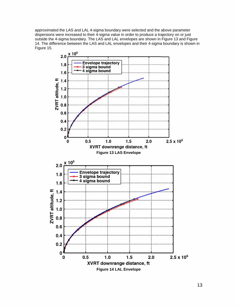
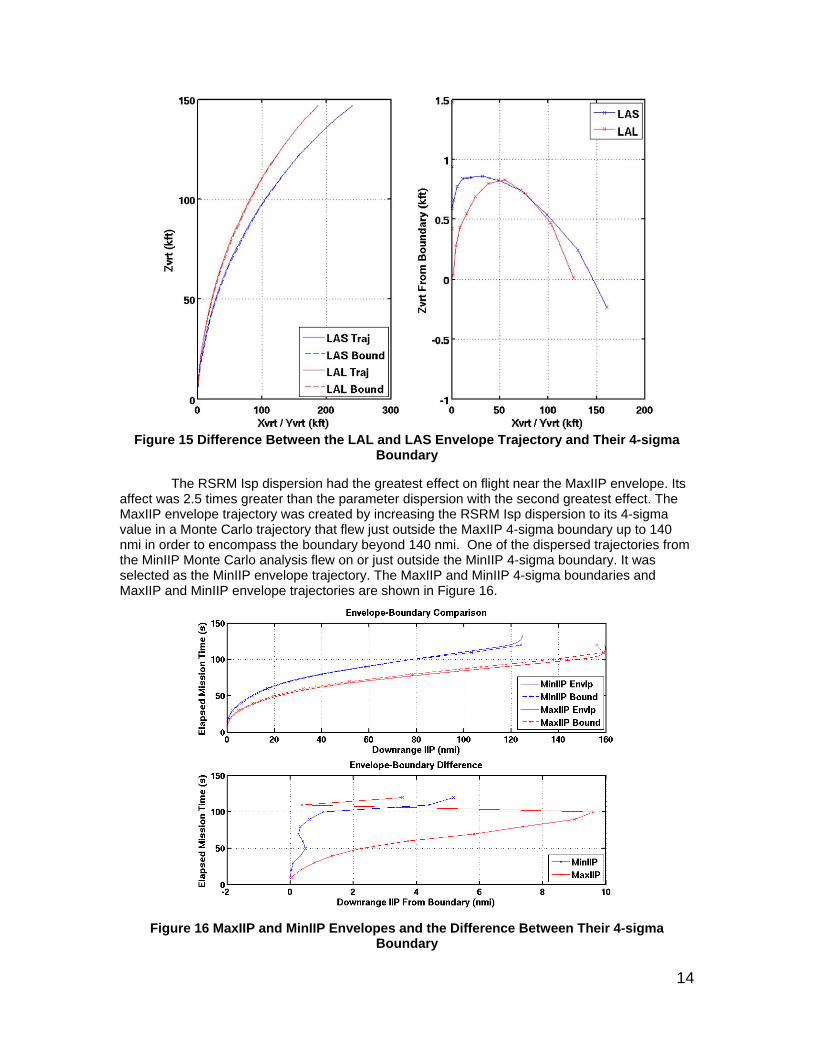
approximated the LAS and LAL 4-sigma boundary were selected and the above parameter dispersions were increased to their 4-sigma value in order to produce a trajectory on or just outside the 4-sigma boundary. The LAS and LAL envelopes are shown in Figure 13 and Figure 14. The difference between the LAS and LAL envelopes and their 4-sigma boundary is shown in Figure 15.

Figure 13 LAS Envelope

Figure 14 LAL Envelope

14

Figure 15 Difference Between the LAL and LAS Envelope Trajectory and Their 4-sigma

Boundary

The RSRM Isp dispersion had the greatest effect on flight near the MaxIIP envelope. Its affect was 2.5 times greater than the parameter dispersion with the second greatest effect. The MaxIIP envelope trajectory was created by increasing the RSRM Isp dispersion to its 4-sigma value in a Monte Carlo trajectory that flew just outside the MaxIIP 4-sigma boundary up to 140 nmi in order to encompass the boundary beyond 140 nmi. One of the dispersed trajectories from the MinIIP Monte Carlo analysis flew on or just outside the MinIIP 4-sigma boundary. It was selected as the MinIIP envelope trajectory. The MaxIIP and MinIIP 4-sigma boundaries and MaxIIP and MinIIP envelope trajectories are shown in Figure 16.

Figure 16 MaxIIP and MinIIP Envelopes and the Difference Between Their 4-sigma

Boundary

15

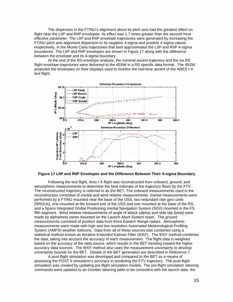
The dispersion in the FTINU’s alignment about its pitch axis had the greatest effect on flight near the LIIP and RIIP envelopes. Its effect was 1.7 times greater than the second most effective parameter. The LIIP and RIIP envelope trajectories were generated by increasing the FTINU pitch axis alignment dispersion to its negative 4-sigma and positive 4-sigma values, respectively, in the Monte Carlo trajectories that best approximated the LIIP and RIIP 4-sigma boundaries. The LIIP and RIIP envelopes are shown in Figure 17 along with the difference between the envelope and its 4-sigma boundary.

At the end of the RS envelope analysis, the nominal ascent trajectory and the six RS flight envelope trajectories were delivered to the 45SW in a RS specific data format. The 45SW projected the envelopes on their displays used to monitor the real-time ascent of the ARES I-X test flight.

Figure 17 LIIP and RIIP Envelopes and the Difference Between Their 4-sigma Boundary

Following the test flight, Ares I-X flight was reconstructed from onboard, ground, and atmospheric measurements to determine the best estimate of the trajectory flown by the FTV. The reconstructed trajectory is referred to as the BET. The onboard measurements used in the reconstruction consisted of inertial and wind relative measurements. Inertial measurements were performed by a FTINU mounted near the base of the USS, two redundant rate gyro units (RRGUs), one mounted at the forward end of the USS and one mounted at the base of the RS, and a Space Integrated Global Positioning Inertial Navigation System (SIGI) mounted in the FS fifth segment. Wind relative measurements of angle of attack (alpha) and side slip (beta) were made by alpha/beta vanes mounted on the Launch Abort System tower. The ground measurements consisted of position data from three Eastern Range radars. Atmospheric measurements were made with high and low resolution Automated Meteorological Profiling System (AMPS) weather balloons. Data from all of these sources was combined using a statistical method known as Iterative Extended Kalman Filter (IEKF). The IEKF method combines the data, taking into account the accuracy of each measurement. The flight data is weighted based on the accuracy of the data source, which results in the BET trending toward the higher accuracy data sources. The IEKF method also uses the measurement uncertainty to develop uncertainty bounds for the BET. Details of the BET generation are described in Reference 7.

A post-flight simulation was developed and compared to the BET as a means of assessing the POST II simulation’s accuracy in predicting the FTV trajectory. The post-flight simulation was created by updating pre-flight simulation models. The pre-flight simulation steering commands were updated to an October steering table to be consistent with the launch date, the

16

atmosphere (density and winds) was updated to the day of launch atmosphere reconstructed from balloon data, and the RSRM thrust and FTV weight versus time data were updated to values reconstructed from flight data.

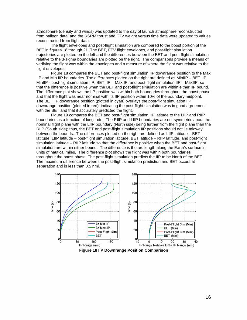
The flight envelopes and post-flight simulation are compared to the boost portion of the BET in figures 18 through 21. The BET, FTV flight envelopes, and post-flight simulation trajectories are plotted on the left and the differences between the BET and post-flight simulation relative to the 3-sigma boundaries are plotted on the right. The comparisons provide a means of verifying the flight was within the envelopes and a measure of where the flight was relative to the flight envelopes.

Figure 18 compares the BET and post-flight simulation IIP downrange position to the Max IIP and Min IIP boundaries. The differences plotted on the right are defined as MinIIP – BET IIP, MinIIP - post-flight simulation IIP, BET IIP – MaxIIP, and post-flight simulation IIP – MaxIIP, so that the difference is positive when the BET and post-flight simulation are within either IIP bound. The difference plot shows the IIP position was within both boundaries throughout the boost phase and that the flight was near nominal with its IIP position within 10% of the boundary midpoint. The BET IIP downrange position (plotted in cyan) overlays the post-flight simulation IIP downrange position (plotted in red), indicating the post-flight simulation was in good agreement with the BET and that it accurately predicted the flight.

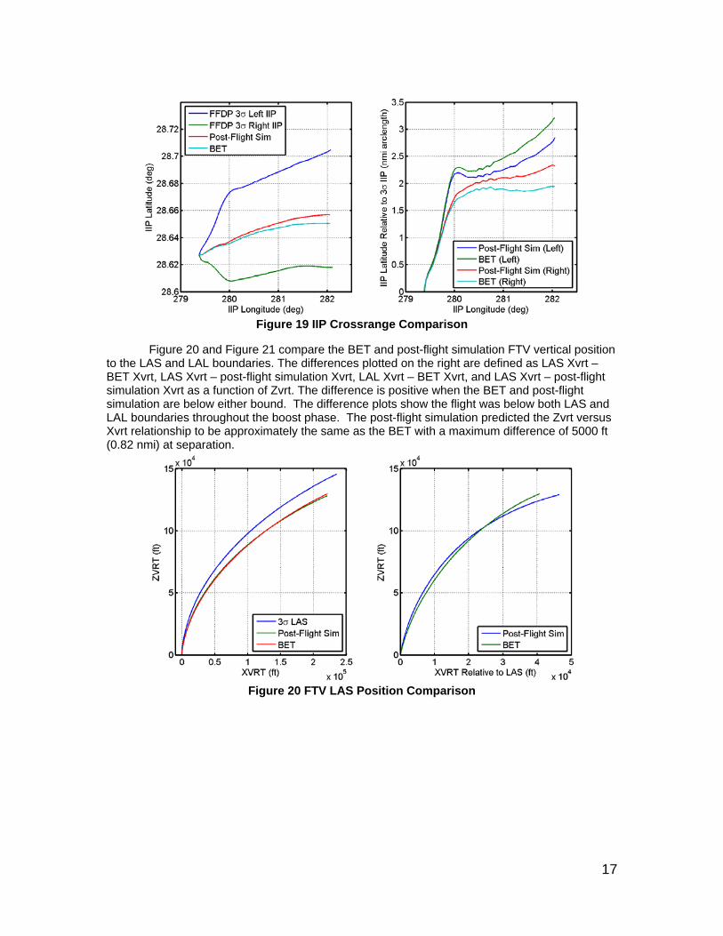
Figure 19 compares the BET and post-flight simulation IIP latitude to the LIIP and RIIP boundaries as a function of longitude. The RIIP and LIIP boundaries are not symmetric about the nominal flight plane with the LIIP boundary (North side) being further from the flight plane than the RIIP (South side); thus, the BET and post-flight simulation IIP positions should not lie midway between the bounds. The differences plotted on the right are defined as LIIP latitude – BET latitude, LIIP latitude – post-flight simulation latitude, BET latitude – RIIP latitude, and post-flight simulation latitude – RIIP latitude so that the difference is positive when the BET and post-flight simulation are within either bound. The difference is the arc length along the Earth’s surface in units of nautical miles. The difference plot shows the flight was within both boundaries throughout the boost phase. The post-flight simulation predicts the IIP to be North of the BET. The maximum difference between the post-flight simulation prediction and BET occurs at separation and is less than 0.5 nmi.

Figure 18 IIP Downrange Position Comparison

17

Figure 19 IIP Crossrange Comparison

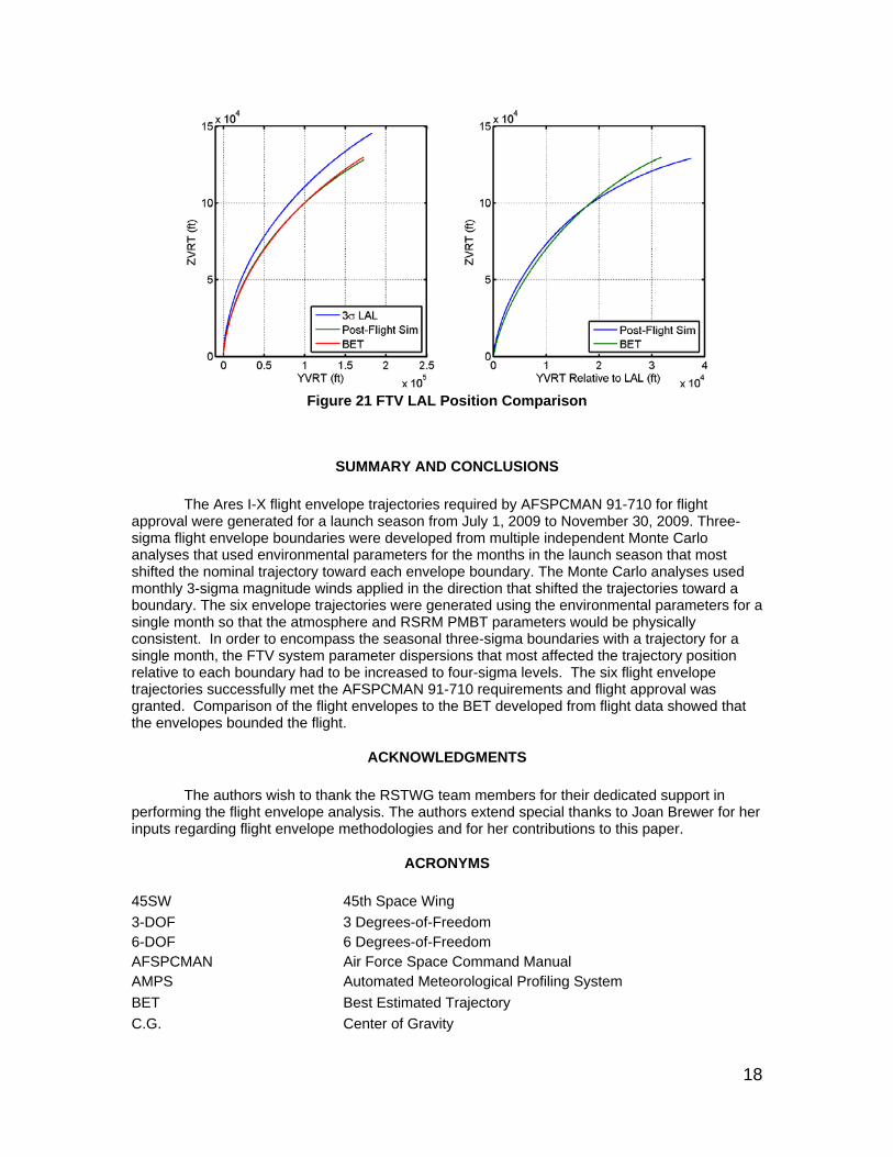
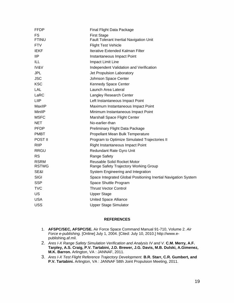
Figure 20 and Figure 21 compare the BET and post-flight simulation FTV vertical position to the LAS and LAL boundaries. The differences plotted on the right are defined as LAS Xvrt – BET Xvrt, LAS Xvrt – post-flight simulation Xvrt, LAL Xvrt – BET Xvrt, and LAS Xvrt – post-flight simulation Xvrt as a function of Zvrt. The difference is positive when the BET and post-flight simulation are below either bound. The difference plots show the flight was below both LAS and LAL boundaries throughout the boost phase. The post-flight simulation predicted the Zvrt versus Xvrt relationship to be approximately the same as the BET with a maximum difference of 5000 ft (0.82 nmi) at separation.

Figure 20 FTV LAS Position Comparison

18

Figure 21 FTV LAL Position Comparison

SUMMARY AND CONCLUSIONS

The Ares I-X flight envelope trajectories required by AFSPCMAN 91-710 for flight approval were generated for a launch season from July 1, 2009 to November 30, 2009. Three-sigma flight envelope boundaries were developed from multiple independent Monte Carlo analyses that used environmental parameters for the months in the launch season that most shifted the nominal trajectory toward each envelope boundary. The Monte Carlo analyses used monthly 3-sigma magnitude winds applied in the direction that shifted the trajectories toward a boundary. The six envelope trajectories were generated using the environmental parameters for a single month so that the atmosphere and RSRM PMBT parameters would be physically consistent. In order to encompass the seasonal three-sigma boundaries with a trajectory for a single month, the FTV system parameter dispersions that most affected the trajectory position relative to each boundary had to be increased to four-sigma levels. The six flight envelope trajectories successfully met the AFSPCMAN 91-710 requirements and flight approval was granted. Comparison of the flight envelopes to the BET developed from flight data showed that the envelopes bounded the flight.

ACKNOWLEDGMENTS

The authors wish to thank the RSTWG team members for their dedicated support in performing the flight envelope analysis. The authors extend special thanks to Joan Brewer for her inputs regarding flight envelope methodologies and for her contributions to this paper.

ACRONYMS

45SW 45th Space Wing

3-DOF 3 Degrees-of-Freedom 6-DOF 6 Degrees-of-Freedom AFSPCMAN Air Force Space Command Manual AMPS Automated Meteorological Profiling System

BET Best Estimated Trajectory

C.G. Center of Gravity

19

FFDP Final Flight Data Package

FS First Stage FTINU Fault Tolerant Inertial Navigation Unit

FTV Flight Test Vehicle

IEKF Iterative Extended Kalman Filter

IIP Instantaneous Impact Point

ILL Impact Limit Line

IV&V Independent Validation and Verification

JPL Jet Propulsion Laboratory

JSC Johnson Space Center

KSC Kennedy Space Center

LAL Launch Area Lateral

LaRC Langley Research Center

LIIP Left Instantaneous Impact Point

MaxIIP Maximum Instantaneous Impact Point

MinIIP Minimum Instantaneous Impact Point

MSFC Marshall Space Flight Center

NET No-earlier-than

PFDP Preliminary Flight Data Package

PMBT Propellant Mean Bulk Temperature

POST II Program to Optimize Simulated Trajectories II

RIIP Right Instantaneous Impact Point

RRGU Redundant Rate Gyro Unit

RS Range Safety

RSRM Reusable Solid Rocket Motor RSTWG Range Safety Trajectory Working Group

SE&I System Engineering and Integration

SIGI Space Integrated Global Positioning Inertial Navigation System

SSP Space Shuttle Program

TVC Thrust Vector Control

US Upper Stage

USA United Space Alliance

USS Upper Stage Simulator

REFERENCES

1. AFSPC/SEC, AFSPC/SE. Air Force Space Command Manual 91-710, Volume 2. Air Force e-publishing. [Online] July 1, 2004. [Cited: July 10, 2010.] http://www.e-publishing.af.mil.

2. Ares I-X Range Safety Simulation Verification and Analysis IV and V. C.M. Merry, A.F. Tarpley, A.S. Craig, P.V. Tartabini, J.D. Brewer, J.G. Davis, M.B. Dulski, A.Gimenez, M.K. Barron. Arlington, VA : JANNAF, 2011.

3. Ares I-X Test Flight Reference Trajectory Development. B.R. Starr, C.R. Gumbert, and P.V. Tartabini. Arlington, VA : JANNAF 58th Joint Propulsion Meeting, 2011.

20

4. S.A. Striepe, R.W. Powell, P.N. Desai, E.M. Queen, G.L. Brauer, D.E. Cornick, D.W. Olson, F.M. Petersen. Program to Optimize Simulated Trajectories (POST II) Utilization Manual, Volume II, Version 1.1.6.G. Denver, CO : NASA, 2002.

5. Falls, L.W. Normal Probabilities for Cape Kennedy Wind Components - Monthly Reference Periods for all Flight Azimuths - Altitudes 0 to 70 Kilometers. Huntsville, AL : NASA Marshall Space FLight Center, April 16, 1973. NASA TM X-64771.

6. NSTS 08209, Volume I, Revison B. Shuttle Performance Assessment Databook. Houston TX : NASA Johnson Space FLight Center, 1999.

7. Ares I-X Best Estimated Trajectory Analysis and Results. C.D. Karlgaard, R.E. Beck, B.R. Starr, S.D. Derry, J.M. Brandon, A.D. Olds . Arlington, VA : JANNAF, 2011. JANNAF-1961.