ari lehto- quantization of keplerian systems

8/3/2019 Ari Lehto- Quantization of Keplerian systems

http://slidepdf.com/reader/full/ari-lehto-quantization-of-keplerian-systems 1/23

Quantization of Keplerian systems

Ari Lehto

Helsinki University of Technology Laboratory of Materials Science

P.O. Box 6200, FIN-02015 TKK

Abstract

A mathematical model is given for the occurrence of preferred orbits and orbital

velocities in a Keplerian system. The result can be extended into energies and

other properties of physical systems. The values given by the model fit closely

with observations if the Planck scale is chosen as origin and the process

considered as volumetric doubling in 3- and 4-dimensions. Examples of

possible period tripling are also given. Comparison is made with the properties

of the basic elementary particles, the Solar system and other physical

phenomena.

PACS numbers: 04.20.Gz, 05.45.-a, 05.45.Mt, 10

1 INTRODUCTION

Connection between the Planck scale and the real world has been long sought for. The

problem is in the extreme values of the Planck scale physical quantities. The Planck energy

E o=1022

MeV is far too large for any elementary particle, the Planck length l o=10-35

mcorrespondingly far too small for any real object, and the Planck period τ o=10-43 s is

extremely short for any real world event.

A process generating subharmonics instead of higher harmonics would decrease the Planck

energy in a natural way by bringing about lower energy levels. One such a process is period

doubling, a common property of non-linear dynamical systems. This type of a process creates

a series of doubling periods and correspondingly halving frequencies and energies according

to E=h/ τ . A series of doubling lengths (l=cτ ) is borne, too. Period tripling, quadrupling etc.

are also general properties of nonlinear dynamical systems.

It has been shown (Lehto 1990) that several stationary properties of matter coincide with

values calculated from the Planck scale by 3- and 4-dimensional volumetric doubling, a form

of period doubling. The perceived values of physical quantities seem to be cube roots of thecorresponding volumes, save the electric charge squared (proportional to electrostatic energy),

which is a fourth root.

In this article we examine properties of a non-linear system in terms of period τ rather than

continuous time t . The best known example of such a formulation is Kepler’s law r 3=aτ

2,

where r is the radius of the orbit, a a constant and τ the period of revolution.

We formulate a differential equation for a test object under a central force field by utilizing

Kepler’s law and give a numerical solution demonstrating the volumetric doubling and

quantization of orbital velocity. The preferred orbits thus obtained can also be expressed in

terms of energy, magnetic moment and temperature. The elementary electric charge is

obtained from the Planck charge by corresponding volumetric doubling in four dimensions.The theoretical results are compared with observations.



2

2 THEORY AND DEFINITIONS

2.1 Preferred periods in a Keplerian system

Kepler’s law tells that r 3=τ

2 (omitting the constant of proportionality). Solving for r and

taking the second derivative with respect to period τ one obtains

(1)

where a is a constant. By again applying Kepler’s law, Eq. (1) can be written in the form

(2)

Equation (2) is formally equation of motion in terms of period of

an oscillator, whose spring constant is inversely proportional to

period squared, i.e. a/ τ

2

. This means that the oscillations slowdown with increasing period.

Direct solution of Eq. (2) would result in negative values of r and

therefore we rewrite Eq. (2) as follows:

(3)

(4)

The necessary requirement for circular motion is 90o phase difference between the x- and y-components. We shall now proceed with solving equations (3) and (4) simultaneously for a

setting shown in figure 1 and reconstruct the radius using the Pythagorean theorem

r z =sqrt(x2+y

2 ). The test object

is initially located at (0, yo=1)

and given an initial velocity

(v xo, v yo=0). Equations are

solved starting from initial

period τ =1 and a=46.47014.

The initial x-component of

velocity is v xo=sqrt(a).

Figure 2 is a plot of asimultaneous numerical

solution to Eq’s (3) and (4)

showing radius r as function of

period τ . One can see that there

are plateaus, where radius r

remains constant over a range

of periods. The ratio of

adjacent radii (plateau values)

is cube root of two.

FIG. 2. Radius as function of period showing ranges of periodwith constant radii.

x

y

v xo

r

yo

FIG.1. Initial setting

of the test object.

0



3

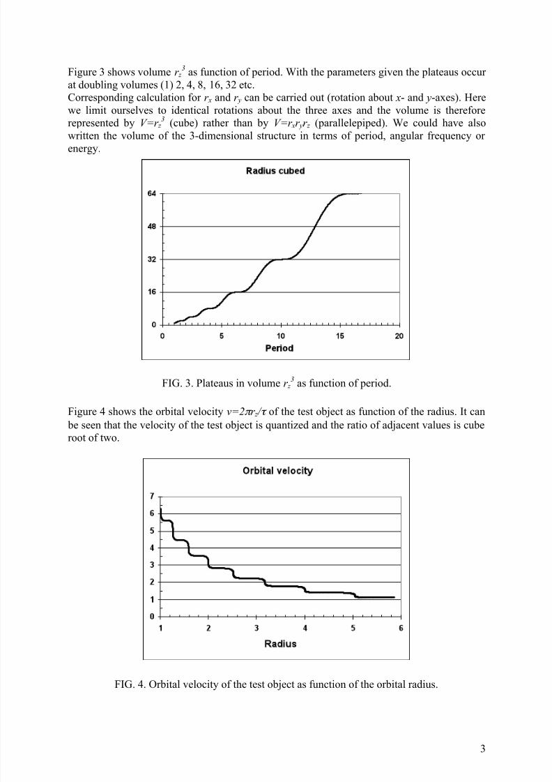
Figure 3 shows volume r z 3

as function of period. With the parameters given the plateaus occur

at doubling volumes (1) 2, 4, 8, 16, 32 etc.

Corresponding calculation for r x and r y can be carried out (rotation about x- and y-axes). Here

we limit ourselves to identical rotations about the three axes and the volume is therefore

represented by V=r z 3 (cube) rather than by V=r xr yr z (parallelepiped). We could have also

written the volume of the 3-dimensional structure in terms of period, angular frequency or energy.

FIG. 3. Plateaus in volume r z 3

as function of period.

Figure 4 shows the orbital velocity v=2π r z / τ of the test object as function of the radius. It can be seen that the velocity of the test object is quantized and the ratio of adjacent values is cube

root of two.

FIG. 4. Orbital velocity of the test object as function of the orbital radius.



4

2.2 4-dimensional doubling

In principle, volumetric doubling in 4-dimensions does not differ from the 3-dimensional

doubling. In this case the value of constant a is a=82.4.

2.3 The Planck scale unitsThe doubling process yields absolute and unadjustable values if the Planck scale is chosen as

origin. We shall now define the Planck scale needed in the comparison of the values given by

the model with observations. The necessary Planck scale units are defined as:

Period (5)

Length (6)

Energy (7)

Charge (8)

Temperature (9)

Velocity c (10)

Units using the elementary electric charge are:

Coulomb energy (11)

Magnetic moment (12)

Magnetic moment (13)

Table I shows the values of the Planck scale units defined by equations (5) to (10) needed in

this study.

Equation (7) is the Planck relation E=hf , where f=1/ τ o. Equation (8) in turn defines the

Planck charge, which is analogous to the Planck mass.

Equations (12) and (13) represent two different geometries, where the Planck length is either

the circumference or the diameter of a magnetic moment current loop, respectively.



5

Table II shows unit values for the

electrostatic energy and magnetic

moment. These units are not strictly

Planck scale units, because the

elementary electric charge is used

instead of the Planck charge. Theseunits must be used because the

particles do not carry the Planck

charge but the elementary electric

charge. It is shown in chapter 3.11.1

how the elementary electric charge is

borne by the doubling process in four

dimensions.

In this model part of the rest energy of charged particles is in their electric fields. The

electrostatic (Coulomb) energy can be calculated from equation (11).

The gravitational constant G is the main source of inaccuracy in the Planck scale units. The

relative standard uncertainty of G is 150 ppm and hence that of the Planck energy, length, and

temperature 75 ppm. The values of the natural constants have been adopted from the NIST

(Mohr and Taylor 2005) table of natural constants.

2.4 Notation

In a three dimensional Cartesian coordinate system volume is V N =2 i .l o

.2 j .l o

.2k .l o=2 i+ j +k

.l o

3=2

N .V o , where V N is the volume of the object, i, j, k numbers of doubling of the edge

lengths and V o the initial or unit volume (e.g. Planck scale cube). Corresponding “volumes”

can be written for any physical quantity derivable from the Planck length.

The total number of doublings N =i+j+k will be denoted by (i, j, k ), which also refers to the

structure of the object. The corresponding notation in 4-d is (i, j, k, l ). The perceived number

of doublings is denoted by n= N /3=(i+j+k )/3 and n= N /4=(i+j+k+l )/4 for 3- and 4-dimensions

correspondingly (cube and fourth roots).

The geometric shape of the object or structure defined by its edges is normally parallelepiped but the shape is cubical, if i, j, k or i, j, k, l are all equal.

The charge squared (qn2) with n=9.75 is called the elementary electric charge (squared) and

denoted by e2.

Magnetic moment will be denoted by µ and defined classically as current times loop area, or

µ =iA.

The rest energy of the electron can be related to a single Planck energy sublevel. This kind of

a particle will be called single-level particle. The corresponding Planck energy is denoted by

E o. Particles, whose rest energy is determined by the sum energy of two sublevels, will be

called sum-level particles. The corresponding Planck energy is denoted by E os. Sublevel

means any energy level obtained from the Planck energy by the frequency ( f=1/ τ ) halving or period doubling process.



6

2.5 Basic formulae

The preferred orbits enable us to derive formulae for physical quantities corresponding to the

quantization. Preferred energies can be calculated by using the Planck relation E=hf=hc/l o

and temperatures by T=E/k (k =Boltzmann’s constant). Magnetic moment can be calculated

from µ =iA (current loop) by the 3-dimensional doubling process and electric charge from the

Planck charge q=sqrt(4πε ohc) by the four dimensional inverse doubling (i.e. halving, negative

exponent) process. Because energy is proportional to charge squared, we calculate the

subcharges using the Planck charge squared. The basic formulae are:

Energy level (3-d) (14)

Energy level (4-d) (15)

Charge squared (4-d) (16)

Magnetic moment (3-d) (17)

Length (3-d) (18)

Period (3-d) (19)

Temperature (3-d) (20)

Velocity (3-d) (21)

Equation (21) can be derived as follows: v i j=l i / τ j=2 il o /2 j

τ o=2 i - jl o / τ o=2 i - j

c=2 - nc , where c

is the speed of light and l o/τ o=c according to equation (6).

Equations (14) to (21) can be written as one constitutive equation:

(22)

where X o is any Planck scale unit.

2.6 Separation of adjacent levels

In the three dimensional system the adjacent values X i=2i X o and X j=2

j X o ( j=i+0.333) are

separated by a factor of 2

0.333

, which means that ( X j- X i)/ X i=260000 ppm and ( X i- X j)/ X i=210000 ppm. The separation is correspondingly 190000 ppm and 160000 ppm in four

dimensions. X is any quantity in equations (14)-(21). Period tripling separates levels by 30.333,

or about 400000 ppm (40%). For the accuracy of the model the difference between the

calculated and experimental values may be compared with the level separations.

2.7 Density of states

The perceived density of the Planck energy sublevels or states, D(E)= Δn/ Δ E n, can be

calculated from equations.(14) and (15) by solving for n. The (absolute) density of states is

(23)



7

where i is 3 or 4 depending on the number of dimensions. Equation (23) shows that the

density of states grows exponentially with n. The perceived Planck scale 3-d density of states

is D(E)=1.4.10-28 (1/eV).

2.8 Superstability

The result of a doubling process is a quantized system with exact values. Consideringtransitions it is customary to talk about initial and final states. From the operational viewpoint

transition to a new state results from an operation on the initial state.

The 1/ x shape of both the Coulomb and gravitational potentials leads to x3=aτ

2dependence of

x on τ (Keplers’s law). Let us now define volume V as V = x3

and consider (the expanding) V as

driving force or an operator V acting on the period τ . According to V =τ 2 the operation is

squaring the period. Let us further assume that there is a shortest period τ o, which doubles (as

space expands) according to τ / τ o=2i, where i is an integer.

The first operation of V on τ / τ o yields V o(τ / τ o)=21 (where o means operation), the second

operation is V o(V o(τ / τ o))=(21)2=2

2, the third V o[V o(V o(τ / τ o))]=(2

2)2=2

4, the fourth

V o{V o[V o(V o (τ / τ o))]}=(24)2=2

8and so forth. The resulting periods can be represented as

(24)

where i is an integer. This is the result of functional iteration leading to superstable periods, as

shown by Feigenbaum (1980). The total number of doublings is of the form N =2i.

2.9 Particle creation

Electron-positron pair creation from a 1.022 MeV

gamma quantum is perhaps the best known example of

materialization of energy. We assume that this type of a pair conversion process is generally valid and

applicable to the Planck energy sublevels obtained by

the volumetric halving process. The particle production

principle is illustrated in figure 5. A single sublevel

and a double level split into a pair of particles.

Double level is either a sum or difference of two

sublevels. For the nucleons we consider the double

level as a sum level.

2.10 Magnetic moment

Let us now define the unit magnetic moment

µ ο as a classical current loop in the Planck

scale. By definition magnetic moment equals

current times the loop area. The loop current is

obtained by dividing the elementary charge e

by the period of orbital revolution. Two

different loops, shown in figure 6, are defined:

a) the orbital type denoted by µ o orb with the

Planck length l o as the circumference, and b)

the radial type denoted by µ o rad with half of

the Planck length as the diameter of the loop.This geometry corresponds to a potential well

Single level

Double level

Particle

pair

FIG. 5. Production of particle pairs.

Particle

pair



8

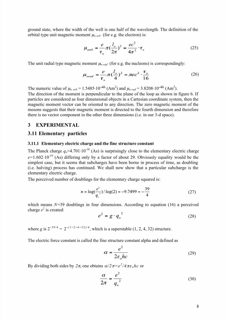
ground state, where the width of the well is one half of the wavelength. The definition of the

orbital type unit magnetic moment µ o orb (for e.g. the electron) is:

(25)

The unit radial type magnetic moment µ o rad (for e.g. the nucleons) is correspondingly:

(26)

The numeric value of µ o orb = 1.5485.10-46 (Am2) and µ o rad = 3.8208.10-46 (Am2).

The direction of the moment is perpendicular to the plane of the loop as shown in figure 6. If

particles are considered as four dimensional objects in a Cartesian coordinate system, then the

magnetic moment vector can be oriented to any direction. The zero magnetic moment of the

mesons suggests that their magnetic moment is directed to the fourth dimension and therefore

there is no vector component in the other three dimensions (i.e. in our 3-d space).

3 EXPERIMENTAL

3.11 Elementary particles

3.11.1 Elementary electric charge and the fine structure constant

The Planck charge qo=4.701.10-18

(As) is surprisingly close to the elementary electric charge

e=1.602.10-19 (As) differing only by a factor of about 29. Obviously equality would be the

simplest case, but it seems that subcharges have been borne in process of time, as doubling

(i.e. halving) process has continued. We shall now show that a particular subcharge is theelementary electric charge.

The perceived number of doublings for the elementary charge squared is:

(27)

which means N =39 doublings in four dimensions. According to equation (16) a perceived

charge e2

is created:

(28)

where g is 2 - 3 9 / 4 = 2 - ( 1 + 2 + 4 + 3 2 ) / 4, which is a superstable (1, 2, 4, 32) structure.

The electric force constant is called the fine structure constant alpha and defined as

(29)

By dividing both sides by 2π , one obtains α /2π =e2 /4πε ohc or

(30)



9

which is the ratio of the elementary charge and the Planck charge squared. We further obtain

Since e2

/qo

2

= 2- 3 9 / 4

, the inverse of the fine structure constant α obtains a value of α - 1

=23 9 / 4 /2π = 137.045. The difference to the recommended value is 65 ppm.

The value of the elementary charge is obtained from Eq. (28):

e = 1.60213.10

-19(As), (31)

which differs by 30 ppm from the recommended value.

The process of volume doubling may also produce other values for the force constants. Some

of these have been calculated (Lehto 1990).

3.12 Rest energy and magnetic moment

3.12.1 Charged leptons

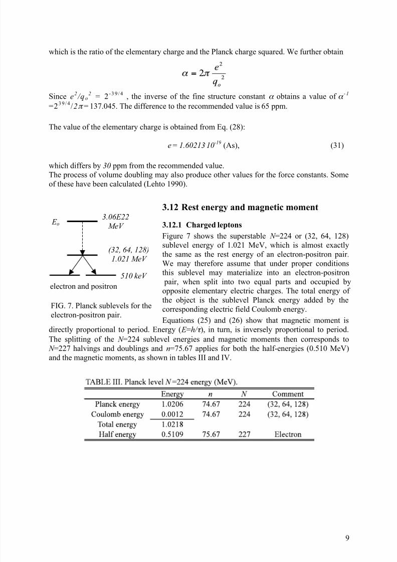
Figure 7 shows the superstable N =224 or (32, 64, 128)

sublevel energy of 1.021 MeV, which is almost exactly

the same as the rest energy of an electron-positron pair.

We may therefore assume that under proper conditions

this sublevel may materialize into an electron-positron

pair, when split into two equal parts and occupied by

opposite elementary electric charges. The total energy of

the object is the sublevel Planck energy added by the

corresponding electric field Coulomb energy.

Equations (25) and (26) show that magnetic moment is

directly proportional to period. Energy ( E =h/ τ ), in turn, is inversely proportional to period.

The splitting of the N =224 sublevel energies and magnetic moments then corresponds to

N =227 halvings and doublings and n=75.67 applies for both the half-energies (0.510 MeV)

and the magnetic moments, as shown in tables III and IV.

E o 3.06E22

MeV

(32, 64, 128)1.021 MeV

electron and positron

510 keV

FIG. 7. Planck sublevels for the

electron-positron pair.



10

The model for an electron-positron pair is simply the Planck 1.021 MeV sublevel occupied by

opposite elementary electric charges. The differences between the calculated and

experimental values may be compared to the separation of the theoretical 3-d sublevels in

chapter 2.6 showing that the measured values are very close to the calculated ones.

Table V shows the structures of the electron-positron pair and the muon. The muon rest

energy 105.6 MeV is close to the uncharged n=68 Planck level ( E =103.7 MeV).

The rest energy of the heavy lepton τ (1777) does not correspond to any single Planck level.

However, the energy difference

between E os series level n=63.75and E o series level n=63 is

1776.3 MeV.

Table V also shows that the

muon components can be

transformed into the electron-

positron pair components by a

three dimensional doubling, where i=64 becomes i=32. The N =224 or 1.021 MeV level can

further split into two 0.511 MeV levels. Because there is only one elementary charge

available the other 0.511 MeV level remains unoccupied and only an electron appears.

Electron magnetic moment anomalyThe magnetic moment µ of a particle is traditionally considered as resulting from the charge

e, mass m and an internal spin S (= h/2π ) of the particle:

(32)

where eS/2m is called a magneton (either Bohr or nuclear depending on the value of m). The

dimensionless number g s is (experimental) gyromagnetic ratio thought to reflect the internal

structure of the particle. The values of g s for the electron, proton and neutron are –1.001,

+2.793 and –1.913 respectively. The measured value of the electron magnetic moment is a

little larger than the Bohr magneton µ B=eS/2me . Magnetic moment anomaly is defined asae=│µ e│ / µ B -1 , where │µ e│ is the measured electron magnetic moment. The anomaly can

be measured very accurately and its current accepted value is ae = 0.00116.

In this model the magnetic moment anomaly is obtained by replacing the Bohr magneton by

the magnetic moment value given in table IV for the electron. One obtains

(33)

which is negative and about one tenth of the classical anomaly. The value of ae differs by 160

ppm from unity. This discrepancy may be partly due to the inaccuracy of G in the Planck

mass and hence in the unit magnetic moment. In principle the doubling process is exact.



11

3.12.2 Neutrino

The Planck energy level system can be considered as a multi-dimensional lattice, because the

energy values are fixed and a geometric structure or a shape can be assigned to. The role of a

neutrino in particle processes within this lattice may be considered as analogous to the role of

phonons in electronic transitions in crystal lattices, namely the transfer of momentum to the

surrounding lattice as a whole.

3.12.3 Mesons

Table VI shows the rest energies of

some meson pairs as compared to

the corresponding Planck sublevel

energies. An overall agreement is

found.

It is customary to consider pions

and kaons as triplets and figure 8

shows that a Planck sublevel can be

split into meson triplets. Energy

level N =4*66=264 splits into pions

and N =3*65.33=196 into kaons.

Note that only the three dimensional part of the kaons is perceived, which makes a strange

distinction between these particle triplets. This is pair production with a neutral particle.

3.12.4 Pion decay

The charged pions decay into muons. Table VII shows that in the decay process the total

number N=4n of doublings increases by one (from 271 to 272) or l from 15=16-1 to 16.

π- π

+π

o

π-+π++πo

= 414.2 MeV

N = (66, 66, 66, 66), E = 414.8 MeV

N = (65, 65, 66, 0) , E = 1488 MeV

K ++ K

-+ K

o =1485 MeV

K - K +K o

FIG. 8. Pion and kaon triplets and corresponding total number of

doublings. The kaon triplet is perceived as a three dimensional object.



12

3.12.5 Nucleons

The leptons and baryons differ from one another in that the leptons are considered as

structureless pointlike particles, whereas the baryons have measurable size and some kind of

an internal structure. This difference is also reflected in the way their rest energies and

magnetic moments are borne in the doubling process.

The nucleon pair can be generated from sum energy level E os as shown in figure 9. The (64,

64, 64, 64) sublevel with 2-64. E os = 1874.6 MeV energy splits into two 937.3 MeV energy

levels. The (64, 64, 64, 64)-level magnetic moment correspondingly doubles into two 65-level

magnetic moments.

The experimental rest energies of the proton and neutron are 938.27 MeV and 939.57 MeV

respectively. Table VIII shows that 937.31 MeV energy is a little short of the rest energies of

the nucleons. If we attach a superstable (32, 64, 128) uncharged sublevel structure and energy

to the 937.31 MeV level, a very close agreement between the calculated and measured proton

rest energies is obtained.

E os 3.46E22MeV

(64, 64, 64, 64)

nucleons

(65, 65, 65, 65)

937.3 MeV

FIG. 9. Planck sublevels for the nucleons from sum energy.

sum

energy E o

E o /2

3.06E22MeV



13

The measured difference between the rest energies of the neutron and the proton is 1.28 MeV.

Table VIII shows that this energy corresponds to n=74.33 or N =223 sublevel energy, adjacent

to the superstable N =224 sublevel. The elementary

electric charges can be attached to the 937.31 MeV

structure by adding an electron-positron pair structure

with one or two charges.The N =192 or (64, 64, 64, 64) radial type magnetic

moment is 7.0482.10-27 Am2. If this value is multiplied

by two (corresponding to (65, 65, 65, 65) structure

obtained by doubling) the magnetic moment of a proton

is obtained, as shown in table IX.

According to measurements neutron’s charge is divided

into a positively charged inner layer and a negatively

charged outer layer. There are thus two current loops of

opposite magnetic moments. The negative loop has

larger magnetic moment than the positive one and the total (negative) magnetic moment is thesum of the moments of the two loops.

Simplest case is now assumed: The larger loop is identical to the proton’s loop µ p (save the

sign of the charge) and a concentric smaller positive loop µ x is added, as shown in figure 10.

The measured magnetic moment of the neutron is minus 9.6624.10-27 (Am2). The unknown

µ x can now be calculated from µ x = µ p+µ n . It is found that

µ x = 263.33 .µ o rad (34)

or µ x = 2-1.67 .µ p

which shows that the magnitude of µ x results from equation (17), too. Neutron’s magnetic

moment is then:

µ n = (2 63.33 - 2 65.00 ) µ o r a d (35)

and no experimental gyromagnetic ratio is needed. Table IX shows the calculated and

measured magnetic moments of the nucleons.

The experimental magnetic moment of the proton differs from the calculated one by 720 ppm.

The difference for the neutron is 660 ppm.

A sublevel is just an energetic state without any electrical charges. In principle it can beneutral or occupied by one charge or two (opposite) charges. In this model the neutron is

µx

−µ p

- +

FIG. 10. Neutron’s

current loops.



14

neutral, because it hosts two elementary charges forming the magnetic moment current loops

but there is only one positive charge within the proton.

As hydrogen is the most abundant substance in the universe, it is plausible to think that the

negative charge associated with the proton’s positive elementary charge remains attached to

the proton, although rather loosely. The ground state orbital magnetic moment of hydrogen is

the same as electron’s (intrinsic) magnetic moment. This means that the Bohr orbit’s magneticmoment has the same periodic structure as the electron’s magnetic moment.

The special feature with the proton is that the same perceived number of doublings, i.e.

n=65.00, is obtained from both a 3-d and a 4-d object ((65, 65, 65) and (65, 65, 65, 65)).

3.12.6 Baryon decay

Figure 11 shows the observed high probability baryon decays. It can be seen that the decay is

related to structural component changes (right side of figure).

FIG. 11. Baryon decay schematically.

The perceived sigma particle is apparently 3-dimensional, so it decays into the 3-dimensional

part of the nucleons.

3.13 Particle collisions

Figure 12 shows a standard example of proton-antiproton collision producing a ksi particle

pair. The proton-antiproton pair energy corresponds to the Planck energy with N =256.

Corresponding number of doublingsfor the ksi pair is N =254. This

means that two components have

changed by unity.

Figure 13 shows another standard

example of proton-antiproton

collision (cascade).

First a charged pion pair and an eta

particle are borne followed by the

immediate decay of the eta into a

pion triplet.

It can be seen that the doublingtakes place in all four dimensions at the corresponding Planck energy levels.

65.00

64.67

64.166

64.75

64.50

n

(65, 65, 65, 65)

Omega - = Ksi* 20.33

E n (MeV)

937

1115

1181

1326

1670

N

Λ

Σ

Ξ

Ω

(64, 65, 65, 65)

(64, 65, 65, 0)

(64, 64, 65, 65)

Ξ+

Ξ-

p+ p-

N = (64, 64, 64, 64)

N = (63, 63, 64, 64)

FIG. X. Proton-antiproton collision producing two

ksi particles. Doubling occurs in two components.



15

3.14 The Solar system

Equations (18) and (21) yield the model lengths and velocities. Figure 14 shows the distances

FIG. 14. Planets in (r,v) space. The asteroids occupy space around N =42 orbit and N =44 is

empty. Note that N =42 and N =44 are on both sides of Jupiter ( N =43). The N -valuesindicated belong to v in Eq. (21).

π-

π+

π+

π-

ηo

πo

p+

p-

π-+π++ηo

= 828 MeV

π-

+π+

+πo

= 414.2 MeV

N = (65, 65, 65, 65), E = 829.5 MeV

FIG. 13. Proton-antiproton collision cascade showing doubling in all

four dimensions.

N = ( 66, 66, 66, 66), E = 414.8 MeV

p++p

- = 1877 MeV

N = (64, 64, 64, 64), E = 1875 MeV



16

and orbital velocities of the planets in (r,v)-space. The asteroids ( N =42 in equation (21)

occupy the gap between Mars and Jupiter. The observed velocities are consequent values of N from N =38 (Mercury) to N =48 (Pluto) in equation (21) with one exception. There is an

unoccupied orbit with N=44 between Jupiter and Saturn, as if a planet were missing there,

too.

The distances from the Sun have been calculated from equation (18) with the Planck length asorigin.

3.15 Quantized galaxy redshifts

According to the accepted cosmological model space is expanding. This view is based on the

observed redshifts of the galaxies, which is the larger the dimmer (i.e. farther away) the

galaxy is. This observation led to the idea that redshift is due to the Doppler shift, meaning

that all galaxies recess from us the faster the farther away they are.

W.G. Tifft of the University of Arizona has measured redshifts for over twenty-five years

using both optical and radio spectra (at 21 cm wavelength). Careful measurements with large

radio telescopes have given results far exceeding the accuracy of optical measurements. Tifft

(1997) has found out with high S/N ratio that the redshifts are not only quantized but also

variable.

Quantization has been verified by Napier and Guthrie (1996) and Napier (2003). These

observations indicate that the redshift is not due to motion alone.

The most prominent redshift period corresponds to 73 km/s and its half. Practically all Tifft´s

redshift periods follow Eq. (21) and its modification (Lehto-Tifft rule), where cube root is

replaced by ninth root (allowing transitions between redshift states). According to the

cosmological principle all observers anywhere in the universe should observe the same

redshift periods. The origin of the quantized redshift may not necessarily be velocity at all but

an expression of the energetic state of the galaxy. If the volume of the universe is expanding,

then doubling proceeds in process of time, which may explain the variable redshift periodsobserved by Tifft.

3.16 Hydrogen and Deuterium hyperfine structure - period tripling

The radio frequency electromagnetic radiation emitted by Hydrogen and Deuterium hyperfine

transitions, also called ”spin-flip radiation”, can be used e.g. in studies of cosmic abundances

and distributions of these gases. The energy released in the Hydrogen transition is E =5.9 µeV

and appears as f =1420 MHz radio frequency known as the 21 cm Hydrogen line. Deuterium

emits radio waves at an energy of E =1.36 µeV, or f =327 MHz, corresponding to 92 cm

wavelength. Both emissions can be received and analyzed using radio telescopes and related

equipment.

Equation (19) can be written in terms of frequency as

f N =f o.2

-N/3(36)

where f N is the frequency after N period doublings, f o the Planck frequency (=1/τ o) and N the

total (integer) number of doublings.

Equation for period tripling is of the same form as (36) but tripling proceeds in powers of three, as shown in Eq. (37)

f N =f o.

3-N/3

(37)



17

If the hyperfine frequencies belong to a doubling or tripling sequence, then N obs should be an

integer. The observed N obs can be solved for from Eq.’s (36) and (37) by replacing f N with the

observed frequency f obs.

The observed Hydrogen frequency yields N obs=336.015 from Eq. (36), close to integer value

336. The Hydrogen frequency can also be obtained from Eq. (37) with N obs=212.0015, even

closer to an integer value.The Deuterium hyperfine frequency from Eq. (37) corresponds to N obs=216.009 period

triplings, close to integer value 216. The observed Hydrogen and Deuterium frequencies have

been adopted from the IAU list of astronomically important frequencies.

The observed and calculated frequencies are shown in table X together with the relative

deviation of N obs from N , i.e. Diff %=( N obs-N )/ N obs.100 %.

TABLE X. Observed and calculated hyperfine frequencies and the number of doublings and

triplings. Also shown is the relative difference between N obs and N .

Object f obs f N N obs N Diff % MHz MHz integer

Hydrogen 1420.41 1421.20 212.0015 212 0.0007 tripling

1425.16 336.014 336 0.0043 doubling

Deuterium 327.39 328.47 216.009 216 0.0042 tripling

Table X shows that the observed number of triplings is very close to an integer number. The

observed and calculated values of the frequencies differ by about 1 MHz (in tripling), the

calculated frequency being higher in both cases. The calculated tripling frequencies for N-1

and N+1 (nearest to N ) are more than 40% off.

3.17 Cosmic background temperature

The 3K cosmic background radiation corresponds to a black body, whose temperature is 2.73

K. Equation (20) yields T =2.76 K with N =320. The next number of volume doublings

towards colder temperature is N =321, which corresponds to T =2.189 K.

It is interesting note that this temperature is very close to the 2.186 K λ -point of liquid helium4He. This is the temperature, where helium becomes super fluid and its specific heat rises

abruptly. This may be an accidental coincidence, but if it is not, then there might be a physical

explanation. Since superfluidity means frictionlessness (or losslessness), then even a weak

coupling to a driving force at resonant frequency (i.e. Planck sublevel) creates exchange of

energy between helium and the Planck sublevels (like coupled oscillators do).

3.18 Cosmic ray spectrum

The most energetic particles are found in the cosmic rays producing the muon showers. The

energy spectrum of incident particles is shown schematically in figure 15 as function of

energy per nucleus. The vertical axis is particle flux in an arbitrary logarithmic scale. The

puzzling features in the curve are the “knee” at 4.5 PeV and the “ankle” at around 6 EeV, as

pointed out by R. Ehrlich (1999).



18

FIG. 15. The knee and ankle in the cosmic ray spectrum.

Equation (14) yields (from E o) E = 4.4 PeV with N = 128. For N = 96 we obtain 7.1 EeV.

These energies coincide with the knee and ankle energies, as shown in figure 15. The

observed kinetic energies correspond to transitions from N =125 to N =128 sublevel and from

N =93 to N =96 sublevels. It may me predicted that there ought to be another “knee” at N =160

(superstable (32, 64, 64)), corresponding to 2.7.10

3GeV energy.

A review article of the present models of the knee and ankle is presented in Hörandel (2004).

None of the models is based on any type of period doubling.

3.19 Superstability in observations

The decimal part of the perceived number of doublings tells the number of dimensions of the

structure or object, because n=N/3 points to three dimensions and n=N/4 to four dimensions.

This information makes it possible to break the total number of doublings (or halvings) into

components in 3- and 4-dimensions. The objects in table XI are related to structures showing

very high stability over time. The superstability condition N i=2i

is found with all these

objects. Notation “e-p pair magnetic moment” means the sum of the absolute values of the

magnetic moments of a positron and an electron.

TABLE XI. Superstable components of the perceived number (n) of doublings.

n N (3-d) N (4-d) Components

Electron-positron pair (e-p) 74.67 224 224+l (128, 64, 32, l )

e-p pair magnetic moment 74.67 224 224+l (128, 64, 32, l )

Elementary charge squared 9.75 39 (1, 2, 4, 32)

Nucleon pair 64.00 192 256 (64, 64, 64, 64)

Nucleon pair magnetic moment 64.00 192 256 (64, 64, 64, 64)

Hydrogen spin flip 112.00 336 448 (128, 128, 128, 64)

3K CBR 106.67 320 320+l (128, 128, 64, l )

cosmic ray "knee" 42.67 128 128+l (64, 32, 32, l )cosmic ray "ankle" 32.00 96 128 (32, 32, 32, 32)



19

The number of dimensions of the elementary electric charge squared may mean that electric

interactions take place also via the fourth dimension.

3.20 Force ratioIf we assume that the expansion of the universe is connected to the process of volume

doubling then this process should be going on at the present time, too. As no smaller electric

charge is known to exist than the elementary electric charge, we must conclude that the

volume doubling process is presently at halt after N=39 volume doublings in four dimensions.

This means that an extremely stable configuration has been reached.

As comes to the Planck mass the doubling process seems to have halted at the electron-

positron pair after N =224 volume doublings, because no lighter elementary particles are

known to exist.

FIG. 16. Relative dilution of the Planck mass and charge squared as

function of the perceived number n of volume doublings in process of

time. Initial value is taken as 1. Note that 2.74.67=149.33 (n of e-p pair

mass squared).

The Planck mass and charge represent the same energy, because

Gmo2 /l o=qo

2 /4πε ol o

This means that in the beginning the energy gradients, or the gravitational force and the

electrostatic (Coulomb) force were equal.

Because the Planck charge has experienced much fewer volume doublings than the Planck mass, its strength is consequently much larger. Figure 16 shows that the volume doubling



20

process has proceeded much farther with mass than with the electric charge. The difference

between the perceived numbers of doublings is 149.33-9.75=139.58. This means that the

perceived ratio of the forces (which are proportional to mass and charge squared) is 2 (149 .33-

9 . 7 5 )= 10

4 2. This ratio may be interpreted as the perceived order of magnitude ratio of the

present strengths of the electric and gravitational interactions.

The strength of the so-called weak interaction is on the order of 10 -13. This is close to 2 - 1 2 8 / 3

= 1.4.10 - 13, which would relate this interaction to the superstable (32, 32, 64) sublevel.

4 DISCUSSION

The solution of the time-independent Schrödinger’s wave equation is interpreted as the

probability amplitude of finding a particle in space. Time-dependent Schrödinger’s equation

describes temporal evolution of the system and can be related to transitional intensities.

Despite of the extreme usefulness and success of quantum mechanics, it cannot be used to

solve for e.g. the intrinsic properties of the electron, like mass or charge, since they are taken

as given constants in the wave equation.

Period doubling is a well established phenomenon in non-linear systems. It has beenthoroughly studied both experimentally and theoretically. It is also known that nonlinear

systems exhibit universal behavior which can be characterized by the Feigenbaum (1978)

constants. It is period doubling that leads to (deterministic) chaos.

In this article it is shown that a differential equation derived from Kepler’s law results in

preferred values of orbital velocities and radii. For absolute values the Planck scale can be

taken as the origin and doubling extended ad infinitum. The structures thus obtained are

fractal by nature, since they look the same at all scales.

Solution r( τ ) of Eq. (2) is fundamentally different from the classical Kepler’s r( τ ), since the

quantization of the Solar system, i.e. the (r,v)-lattice, is independent of the Sun’s mass, which

only determines the location of the v=sqrt(GM/r) hyperbola in the lattice. The orbital

velocities of the planets seem to have preferred values obtainable directly from the speed of light by a 3-dimensional inverse doubling (i.e. halving) process in this case. The quantized

galaxy redshifts, if interpreted as velocity, behave in the same way (Tifft 1998). This behavior

of the solution of Eq. (2) may suggest a deeper connection between the model and non-linear

processes in the universe.

Perturbations can be taken into account by adding attenuation (or amplification) in Eq. (2)

such that the constant of attenuation b/ τ is inversely proportional to period.

(38)

Several other experimentally determined properties of invariants come into the realm of the

solution of Eq. (2). If the circumference 2π r is regarded as wavelength λ , then also energies

E=hc/ λ become quantized. If the Planck length is taken as the initial λ (i.e. E =Planck energy),

then a good fit with the properties of the basic elementary particles is obtained. Magnetic

moments can be likewise calculated if the elementary charge is given. The electric energy

seems to follow 4-dimensional doubling (or halving) suggesting that the electric interactions

may require more than three dimensions.

According to Eq. (16) the model allows particles to take on other values of the electric charge

than the elementary charge. This possibility should be taken into account in analyzing

experimental particle mass spectra in view of this model. Electrons and protons have very

long lifetimes, which mean that the associated structures are extremely stable.



21

One possible scenario for the superstability is shown in chapter 2.8, where a special subset of

possible doublings is created. Table XI shows that the superstability condition is rather

general. The real physical processes behind the superstability remains unsolved for the time

being.

The rest energies of the electron and the positron are found in the direct sequence of energy

sublevels obtained by the doubling process from the Planck energy. The nucleons seem to becomposite particles, because their rest energy is obtained from a sum energy level.

The magnetic moments of the electron and proton seem to originate from two different

geometries. The unit current loop defining the electron’s magnetic moment is Bohr-type, i.e.

the circumference of the loop is the Planck length whereas the geometry of the proton’s unit

magnetic moment is potential well ground state type (loop diameter is half of the Planck

length).

Spin was originally invented to explain some features of the atomic spectra. It is also used to

explain the existence and magnitude of magnetic moments of particles together with the

associated experimental gyromagnetic ratio, which depends on the internal (largely unknown)

structure of particles. Difficulties with the relation of spin and the internal structure aremanifested in the notorious proton spin problem. In this model it is simply the classical

magnetic moment that determines the magnetic moments of the particles dealt with.

The analysis of the electron magnetic moment anomaly in chapter 3.12 showed that according

to this model the anomaly is negative and much smaller than the classical anomaly.

Nonlinear dynamical systems exhibit doubling, tripling, quarupling and so forth of the

fundamental period. The doubled periods double, tripled periods triple again and so forth and

corresponding frequencies appear. The period tripling process may be responsible for the

hyperfine structures of Hydrogen and Deuterium, as shown in table X.

The superstability condition applies to the electron-positron pair, not the electron or positron

alone. This is interesting in the sense that it is the electron-positron pair that is stable. Thisimplies that the electron and positron always co-exist forming a joint energy-object and being

somehow connected. The pair can be spatially separated in the 3-dimensional world without

altering their invariant properties. Freedom in the 3-dimensional space means that the

connection may be via the fourth dimension.

The nucleons can be thought to originate from a superstable (64, 64, 64, 64) E os sublevel. This

level splits into two nucleons the same way

as the electron and positron are borne. Table

VIII shows that 1.021 MeV of additional

energy is needed in order to obtain themeasured rest energy of the proton. The

corresponding two 511 keV structures are(33, 65, 129), i.e. the electron or positron

structure, but only one of the levels becomes

charged (positively in this case) and can be

thought to produce the (65)-level magnetic

moment of the proton. The neutron seems to

host both charges together with an additional

1.28 MeV energy, which is the N=223 ( E o)

structure. The length corresponding to level

(65) is 265l o=1.5.10-15 m, which is of the

order of the nucleon “size”.

The elementary particle processes seem to be

65.00

64.67

64.3

64.6

Δ E= 108 MeV

65.0

Δ E =136 MeV

E o E os pion energies

muon energies

nucleon

FIG. 17. Pion and muon energies appear intransitions around the nucleon level.



22

governed by the 3-d or 4-d structural changes appearing as changes in the number of

doublings (as e.g. in pion decay into a muon, table VII)

It is known that pions are profusely produced in proton collisions. Figure 17 shows that the

energy level differences around the nucleon (65)-level correspond to the pion and muon

energies. These energies may be transferred to the pion and muon energy levels by resonant

energy transfer.

The distances r n (in A.U.) of the planets from the Sun obey the so called Titius-Bode rule,

found experimentally and not valid beyond Uranus. One form of the rule is r n=n+0.4 in

astronomical units with n=0, 0.3, 0.6, 1.2, 2.4 … (doubling n, n=0 for Mercury). The

difference between the Titius-Bode rule and the model presented in this article is that the

quantized Keplerian system gives absolute values for the allowed orbits (and orbital velocities

in addition).

The cosmic background radiation (CBR) is detected as microwave photons coming from all

over the sky. In quantum systems electromagnetic quanta are emitted during transitions from

a higher energy level to a lower one. The CBR temperature converted into energy of the

photons corresponds to the superstable N=320 sublevel energy. This means that the transitionoccurs from N=319 level to N=320 level, whence the photon energy appears as N=320 level

energy, which is the energy difference of these levels. Corresponding reasoning applies to the

21 cm wavelength of the Hydrogen spin-flip.

W.G. Tifft (1996) has shown that the redshift periods of galaxies may change from one period

to the next (redder) period in a few years. As the thicknesses and diameters of galaxies are

typically 10,000-100,000 light years, no signal traveling at the speed of light would reach the

whole galaxy within years. This implies that a galaxy is some kind of a superstructure and the

change is due to the doubling process concerning the whole structure simultaneously.

According to this model the change must take place in the fourth dimension.

The experimental data suggests that the observer seems to perceive the cube root or the fourth

root of a volume, or the geometric mean of the edge lengths of the corresponding three andfour dimensional geometric structures. This situation may be due to the way we carry out

measurements, which produce scalar values.

References

Ehrlich R. 1999, ”Is there 4.5 PeV neutron line in the cosmic ray spectrum?”, Phys. Rev. D,

60, 073005

Feigenbaum M. J. 1978, “Quantitative universality for a class of nonlinear transformations”,

J. Stat. Phys., vol 19, 1, 25-52

Feigenbaum M. J. 1980, Universal behavior in nonlinear systems, Los Alamos ScienceGuthrie B.N.G. and Napier W.M. 1996, Redshift periodicity in the Local Supercluster,

Astron. Astrophys. 310, 353-370

Hörandel J.R. (2004), Models of the knee in the energy spectrum of cosmic rays,

Astroparticle Physics 21, 241-265

IAU list of astronomically important frequencies, http://www.craf.eu/iaulist.htm (28.07.2008)

Lehto Ari 1984, On (3+3)-Dimensional Discrete Space-Time, University of Helsinki, Report

Series in Physics, HU-P-236

Lehto Ari 1990, Periodic Time and the Stationary Properties of Matter, Chin. J. Phys., 28, 3,

pp. 215-235

Mohr Peter J. and Taylor Barry N. 2005, CODATA Recommended Values of theFundamental Physical Constants: 2002, published in Review of Modern Physics 77, 1



Napier W.M. 2003, A statistical evaluation of anomalous redshift claims, Astrophysics and

Space Science 285: 419-427

Tifft W.G. 1976, Discrete states of redshift and galaxy dynamics I, Astrophysical Journal,

Vol. 206:38-56

Tifft W.G. 1997, Global Redshift Periodicities and Periodicity Variability, Astrophysical

Journal v.485, p.465

ari lehto- quantization of keplerian systems

Documents