Arimed Services Technical information AgencyARLINGTON HALL STATION

ARLINGTON 12 VIRGINIA

CONTR~OL ONLY Oq NOTMc WU~ N OOV3R~iNT WOR GIEMRDRAWINGS, SPECIFICATIONS OR OTHER DT

GOVZM0TPWIURRRMTOP2-A-"WN TH U.S. OVERNO[ENT THEREBY ICRNO KORAN' f T9I ANY OBJAINW!ATUOEVER; AND THE FACT THAT THEG OVEENMWI MAY HAVEC FOMtULATED, FRIE, OR IN ANY WAY SUPPLIED) THESAW DRAWYNCA SPSCUSCATIK, 08 OTlER DATA IS NOT TO BE -aGARDZD BY11MPUCATION OR OTZWIAS I ANY MANNER LSCZNMENG THE HOLDER OR ANY OITHERpUMow tOR 0ATOI, OR COIWEYIM ANY ItIWra OR PERNMON TO MANUFACTURE,,I 01 UL ANY PATENTED DWmKTEAT MAY I ANY WAY BE RELATED THERETO.

PROGRESS REPORT

Study of CO, Absorption SpectraBetween 15 and 18 Microns

BY

ROBERT P. MADDEN F

Work dome in part -mnder coxtract with

SOF NAVAL RESEARCHContract Nonr 2 48 ( 01)

JOHNS HOPKINS UNIVERSITY

LABORATUzA A iTROPHYSICS AND PHYSICAL METEOROLOGY

BALTIMORE 18, MARYLAND

FEBRUARY 1, 1957

51)4L a

ANYq i1k1s twj YZS O4fp

PROGRESS REPORT

Study of CO, Absorption SpectraBetween 15 and 18 Microns

BY

ROBERT P. MADDEN

Work done inp ~rt under contract with~

OFFICE OF NAVAL RESEARCHContract Nour 24f (0 1)

THE JOHN$ HOPKINS UNIVERSITY

LABORATORY OF ASTROPHYSICS AND PHYSICAL METEOROLOGY

BALTIMORE 18, MARYLAND

FEBRUARY 1, 1957

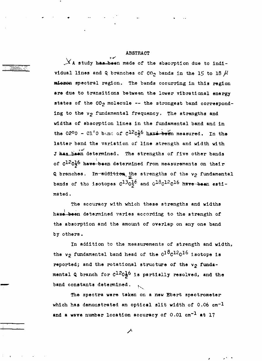
ABSTRACT

,.YA study h.&-b.n made of the absorption due to indi-

vidual lines and Q, branches of CO, bands in the 15 to 18 P

mon spectral region. The bands occurring in this region

are due to transitions between the lower vibrational energy

states of the CO2 molecule -- the strongest band correspond-

ing to the v2 fundamental frequency. The strengths and

widths of absorption lines in the fundamental band and in

the 0200 - 01'0 b.nr of C12 0 6 hx.yg -n measured. In the

latter band the variation of line strength and width with

J "ao.n determined. The strengths of five other bands

of C120 6 have-been determined from measurements on their

Q branches, 1n--aCdttia the strengths of the v2 fundamental

bands of the isotopes C1 3 012 and 01 8C12016 hRve-en esti-

mated.

The accuracy with which these strengths and widths

ha&v4eben determined varies according to the strength of

the absorption and the amount of overlap on any one band

by others.

In addition to the measurements of strength and width,

the V2 fundamental band head of the 01 8 C1201 6 isotope is

reported; and the rotational structure of the v 2 funda-

mental Q branch for C120J 6 is partially resolved, and the

band constants determined.

The spectra were taken on a new Ebert spectrometer

which has demonstrated an optical slit width of 0.06 cm-l

and a wave number location accuracy of 0.01 cm-i at 17

/p

microns. The 1/6 spectrometer utilizes a 3 in. long slit

4 and a 14 in. x 12 in. grating. The absorption by H20 and

CO2 in the optical path of the spectrometer is eliminated

by the removal of these gases. The present experiments

were performed with a slit width of 0.24 mm, correspond-

ing to a spectral slit width of 0.1 cm "1 .

ACKNOWLEDGEMENTS

The author wishes to express his indebtedness to

Professor Strong who has not only been endlessly avail-

able for consultation, and collaborated in solving the

more difficult experimental problems in this work, but

also has been a source of inspiration throughout the

entire program. The author is also much indebted to

Dr. William S. Benedict for his guidance in the inter-

pretation and analysis of the spectra, and the inter-

pretation of the results; also for the use of several

unpublished tables. The author also wishes to thank

Dr. Lewis Kaplan for several helpful suggestions and

the u~e of tables in his possession; and to express

his appreciation to Dr. H. W. Babcock of the Mt. Wil-

son and Palomar Observatories for successfully ruling

the large diffraction grating. Finally, thanks are

due to the entire staff of the Laboratory of Astro-

physics and Physical Meteorology, especially Mr. McClel-

lan and Mr. Brustad, for their generous assistance in

carrying out, and completing, this research.

This work was supported in part by Navy:Contract

Nonr 248(01).

OFa

TABLE OF CONTENTS

Title Page

Abstract

Acknowledgements

I. Introduction

II. Methods of Determining Strengths and Widths

from Absorption Spectra 6

A. Definitions 6

B. Direct Determination 8

C. Direct Determination Using Slit Function

Correc ti ons 9

D. SO Determination for Weak Absorption 10

E. "Curve of Growth" Method 12

F. Method of Wilson and Wells 16

G. Elsasser Band Method 18

III. Experimental Discussion 19

A. Spectrometer 19

(1) Optics 19

(2) Grating 20

(3) Drive and Rotation 21

(4) Alignment Instrument 22

(5) CO2 and H20 Reiroval 22

(6) Calibration 23

(7) Resolution 25

(8) Electronics 26

B. Experimental Set-Up for the Study of C02 26

* - - *dm-*

IV. Data 29

A. Spectra 29 4

B. Analysis of the Spectra 32

(1) 661 - 666 cm "1 Region 33

(2) 624.5 - 629 cm - 1 Region 35

(3) 598 - 613 cm-1 Region 38

(4) Q Branch Measurements 39

V. Discussion of Results 42

A. Line and Band Strengths 42

B. Line Widths 47

VI. Conclusions 49

Bibliography

Tables

Figures

Appendix

I!

I. ImODUCT ION

The object of this research has been to advance the

knowledge of the intensity distribution of gaseous CO2

absorption lines in the spectral region 545 to 667 cm-I.

Such research is amply justified since this region of CO2

absorption plays an important role in the heat balance of1

the earth's atmosphere, and the transmission of infrared

radiation through this atmosphere. In addition, a calcu-

lation2 of the emissivity of CO2 and an understanding of

the role of CO2 in flame emission, both of considerable

military interest, require such measurements.

Three basic quantities may be studied in absorption

spectroscopy: the wavelength position, the strength and

the shape of the absorption. In the following discussion

these will be considered in turn0

Wavelength positions of the individual lines are of

interest since the molecular constants, and the energy

levels for the molecule may be determined from them.,

Little attention has been given to this phase of the prob-

lem in this study since the position of the lines in the

important bands in this region have recently been studied

with good resolution by Blau, etco, 3 and an evaluation of

this and other studios has been made by Benedict.4

Table 1 in a list of the lower vibrational states

of C02, including the upper and lower levels of all the

important transitions of C02 occurring at normal tempera-

ture in tl i 545 to 667 M"I region. Table 2 contains the

2.

band constants which are most useful in the present study.

The only wavelength measurement in these experiments

is the band head determination of the 01'0 - 000 band of

the 01 8 C12 01 6 isotope. Also relative positions of the Q

branch lines for the 01'0 - 000 transition of the C12 0162

isotope were made to determine the band constants for the

q branch. These measurements have not previously been

recorded.

The second basic quantity of interest is the strength

of absorption, from which transition moments may be calcu-

lated. The strength of absorption for a whole band, or the

band strength, may be determined by adding the strengths

of all the lines in the band, This method requires that

all the individual line strengths be observable, but has

ths advantage of yielding the distribution of strength

within the band, The evaluation of strengths of whole

CO2 bands has not been made by adding the strengths of

individual lines since no spectrometer has been available

with sufficient resolution to resolve the overlapping bands.

Methods have been developed 5'6 '7 for determining whole band

strengths from measurements on unresolved bands. Diffi-

culties arise however, if several bands overlap, for it

is impossible to be sure of the separate contributions of

each.

The first investigation of the 15 to 18 micron spec-

tral region in which the CO2 rotational structure was

resolved was made by Martin and Barker. - The resolution

3.

attained, however, was insufficient for" individual line

strength determinations and no intensity analysis was

made. Although several investigators9lOll,12,l3,*4

have measured the total absorption by C02 in the 13 to

18 micron region, they were unable to apportion the proper

share of the total intensity to the separate bands. Re-

cently, Kostkowskil 5 determined the strengths at sle-'ated

tsmperatures of the bands on the high frequency side of

the v2 fundamental at 15 microns. The most recent and

perhaps the best attack on the room temperature intensi-

ties of the bands on the high frequency side of the funda-

mental, and the fundamental itself, has been made by Kap-

lan and Eggers o16 They have made total band measurements

using a low resolving power.

Calculations of expected intensities in the funda-

mental and several other bands, based on available experi-

mental evidencep and assumptions of a molecular model,

have been made by Kaplan 1 ' 1 7 and more recently by Bene-

dictoi 8 A discussion of the agreement between the present

experimental values and Benedlictvs predicted values will

be given.

The third basic quantity to be studied in absorp-

tion spectroscopy is the shape of absorption lines, from

which molecular interaction forces and other broadening

influences may be determined. The width of an absorption

line is a measure of the strength of the broadening influ-

ene

°.

14.

Unfortunately, it is difficult to study the shape

of individual lines at any distance from the line center

in such a crowded spectrum as occurs in the 15 to 18

micron region of C02 absorption. In these experiments,

only the width of the absorption lines was Aeterminable.

Absorption lines are broadened predominantly by

three mechanisms: the natural width, the Doppler effect,

and collision broadening. For C02 in the infrared, the

natural width is negligible compared with that due to the

other two mechanisms. The Doppler effect can be important

at elevated temperatures. At room temperature, however,

the Doppler width for C02 is only .0011 cm-1, while the

width due to collision broadening is about 0.2 cm- 1 at

one atmosphere pressure. Since the Doppler width is inde-

pendent of the pressure, while the collision width is

proportional to the pressure, the Doppler effect can be

neglected in these measurements for pressures greater

than .01 atmos. The range of pressures used in these

experiments was from 0.025 atmosphere to 1 atmosphere.

The collision width of absorption lines cannot be

calculated from Kinetic Theory since the collision diam-

eter for optical interaction is different from the colli-

sion diameter determined from viscosity and conductivity

measurements. Therefore, the collision width must be

determined directly from the spectra.

Ade 119 studied the v2 fundamental of C02 under high

resolution using a grazing incidence grating spectrometer.

5.

He determined what he considered an upper limit of 0.12

cm"1 for the average half-width of the lines in the fund-

amental band. The average half-width for the 2077 co-i

band of CO2 was determined by Benedict and Silverman.2 0

to be .075 cm-1 . Kostkowakil 5 determined the average

half-width f'or the peak of the R branch of the 961 cm-1

band to be 0.084 cm- I .

High resolution is necessary to make measurements

of strength and width on individual absorption lines, and

thus determine the variation of strength and width with

J. In addition, the use of high resolution reduces the

uncertainty in band strength determinations caused by the

overlap of different bandE. The spectrometer used in the

present experiments has available the highest resolution

yet attained in the 15 to 25 micron spectral region, and

measurements on strengths and widths of individual absorp-

tion lines were possible in many cases.

6.

II. MITHODS OF DETERMINING STRENGTHS AND WIDTHS FROMABSORPTION SPECTRA

A study was made of the methods available to reduce

the spectra in order to determine the experimental con-

ditions which yield measurements containing the most ac-

cessible information. The desired quantities are line

and band strengths and line half-widths. These quanti-

ties are defined below.

A. Definitions

The transmission of the gas at frequency v is

defined as T Jo Here 10 is the intensity of

light of frequency v incident on the gas sample; end IV

is the intensity of light of frequency v transmitted by it.

The absorption of the gas at frequency v is defined

as Ao= I-T o

The absorption coefficient at frequency v, kv , is

now defined by the Lambert's Law relation: V- .---

where . is the length of path through the gas sample

over which the light travels, and kv has the dimensions

cm-I . It is assumed that the gas has a uniform density

throughout this path. (If this condition is not satis-

fied, the quantity d =-IV k#) must be integrated

over the whole path.)

The integrated absorption coefficient for an absorp-

tion line is defined as: 5 fkv dv where Vis

the absorption coefficient for that line alone, and S has

the dimensions cm-2 o

7.

The line strength is basically defined as the inte-

grated absorption coefficient per molecule, S/No, where

No is the molecular density of the gas. However, since

the ideal gas law holds for all pressures used in these

experiments, and since all measuremorkts were taken at

one temperature, it is much more useful experimentally to

define the line strength per atmosphere, So, at 3006K by;

So = S/P

where P is the gas pressure in atmospheres, and SO has

the dimensions cm-2/atmos.

The band strength SVu , is then given by:

V/ Z

where the sum is over all lines in the band* and isV,

the line strength of the ith line. 5vS is a most impor-

tant quantity since it has been shown11 to be directly

related to the vibration transition moment by the relation:

3 No V9 (/ V A- 3hc c2(1)

3 hc QVV1

where RV# is the vibrational transition moment

No = molecular density at 1 atmosphere

pressure and 3000K

is 1 for all bands observed in these

experiments

8.

1 for states

2 for all other states

The half-width, 5 , of an absorption line is

defined as one-half the width of the absorption coeffi-

cient curve measured at a height equal to one-half of

the maximum value of the absorption coefficient for that

line. Kinetic Theory, the collision broadening theory

of Lorentz,21 and considerable experimental evidence

leads to the conclusion that the half-width of a colli-

sion-broadened absorption line is proportional to pres-

sure over a wide range of pressures -- and certainly

over the pressure range of these experiments. Accord-

ingly, we define 0, the half-width corrected to

atmospheric pressure at 3000K, by

where P is the pressure in atmospheres of the gas at 300 0 K.

B. Direct Determination

Prom the observed spectra we wish to determine the

physical quantities So, 5 # , and o . This determi-

nation is a straightforward procedure if the resolving

power of the spectrometer is high enough, and the pres-

sure of the gas is adjusted so that: a) No given line

9.

is overlapped by its neighbors., and b) the width of the

line is larga compared with the spectrometer optical alit

width. In this case there would be no distortion of the

true transmission curve by the spectrometer, and by divid-

ing the logarithm of the transmission by the path length

one would obtain the true absorption coefficient. Since

by assumption there is no overlap, the line width could

be measured directly and the strength could be determined

by integrating the absorption coefficient over the wave-

length interval.

Since the experimental conditions necessary to use

such a direct method are seldom realized, it is necessary

to consider other methods which are made possible by sim-

plifying assumptions. These are listed below in order of

the increasing number of assumptions necessary for their

use. The listing is not intended to be exhaus-'ive, but

it contains the techniques which are appropriate for in-

terpreting the present observations.

C. Direct Determination Using Slit Function Corrections

For cases where the requirements for use of direct

determinations can not be met exactly, but can be met

approximately (i.e., conditions require that the line

width be of the same order of magnitude as the optical

slit function of the spectrometer), the above method can

still be used if a correction is made for the "smearing

out" effect of the spectrometer on the spectra. Such

corrections depend on a gvod knowledge of the slit funcon,

10.

defined as:

0,$tensity of light of frequency v passed bysthe slit

OiV 0 J-) = intensity of light of frequency vo passedby the slit

where vo is the frequency setting of the spectrometer,

and v is the frequency in the spectrum.

This slit function is primarily dependent only on

the variable (v-v o and its dependence on this variable

must be known to make the correction mentioned above.

Kostkowski and Bass 2 2 have calculated the appro-

priate corrections to be used in obtaining true S, t ,

and peak absorption from the observed spectrum assuming

a Gaussian slit function. The corrections were calculated

for many values of the ratio of line width to optical slit

width. These corrections are particularly appropriate

for use in this study, since it has been experimentally

confirmed recently by Von Planta, 23 that a Gaussian slit

function is a good approximation in an Ebert type spec-

trometer for the slit widths used here. Figures 1 and 2

show the corrections to be applied to the observed S and

' (calculated from curves of log Tobso) in order to

determine the true S and t . It should be noted that

the correction for b is much greater than the correction

for S under identical experimental circumstances.

D. So Determinaticn for Weak Absorption

When the line width is smaller than the optical slit

width, which is the case if low pressures are required to

11.

separate the spectral structure, it is necessary to turn

to even more indirect methods of determining SO and 60

Of prime importance in these methods is the quantity called

"equivalent widths or W, defined by:

W -fAobsdv

Here the range of integration must begin and end in regions

of zero absorption if the definition is to have meaning,

and it is assumed that there is no overlapping of lines.

The importance of this quantity centers about the fact that

it is independent of the slit wiCth (so long as the slit

function is symmetrical). The integral may extend over

any desired interval if the restrictions mentioned above

are satisfied -- A vobs being the observed absorption in

that interval. Since W is independent of the slit function

it follows that:

=fA, AAbjdc/ (2)

i.e. the integrated observed absorption over any interval

beginning and ending in a region of zero absorption is

equal to the integral of the true absorption over that

interval.

-kvA

Since Av IT -

we have (7-e ) v

&'; | i

12.

Now let kV - 0 o Then:

Um kI -j k =v 5 _QP (3)

Thus if W is measured for a given spectral interval

at many path lengths, and the quantity # is extrapo-

lated to 9 =0 , SO is obtained. This So may be the

strength of one line, or the aggregate strength of many

lines, depending on the spectral interval over which the

absorption was integrated.

This method has two limitations. Firstly, since the

most important measurements to be made are those when the

observed absorption is extremely small, it is difficult

experimentally to obtain accurate measurements. Secondly,

there is no way of determining 6 from such a treatment.

E. "Curve of Growth"Method

In order to determine 9'0 under the condition that

the line width is not large compared to the spectrometer

slit width, and so that measurements on lines of stronger

absorption will be of some help in determining SO, another

method has been developed called the "Curve of Growth"

method. The important assumption made in the use of this

method is that th) shape of the absorption coefficient

curve for any given line is the symmetrical shape calcu-

lated by Lorentz 21 for collision broadening. Lorentz pre-

dicted a Cauchy shaped line given by:

--y 5 )2 (4)/ " r (-v

13.

where 5 and have been defined, and vo is the central

frequency of the line.

While there is some question remaining as to whether

or not the Lorentz shape is correct for frequencies far

from the line center, there is general agreement that the

Lorentz formula predicts the correct shape near the cen-

ter of the line. In particular Benedict 18 has reported

that the Lorentz formula predicts the correct value of

the absorption coefficient at a distance of 1 cm "1 away

from the line center for C02 absorption lines in the 4.7

micron band. Because the absorption measured under all

experimental conditions of this study is negligible at a

distance of 1 cm-1 away from the line center, the assump-

tion of the Lorentz shape for this work seems Justified.

With this assumption the following argument is made:

o 0

If the entire contribution to W is due to a single line,

ex

w'= (I-e 1P[# (1,V - 2.FVO ) 2-0

This integral has been solved5 ' y Ladenburg and Reiche

and the result is:

Ntd 2TT [J tX - a X)

w) 1where X (6)

27-7

14.

J0, Jl are Bessel functions of the 0 and 1 order. For

simplicity this equation may be written:

where F(x) x e-X[J-o( ) - J ax)]

The function F(x) has been tabulated by Stover.24 Fig-

ure 1 is a plot of F(x) VS. X. This function is called

the Ladenburg-Reiche Function.

For the limiting case of x-, o, lim F(x) = x (linearA3 X- O

region)0 Then:

T a ,= 2 _ - (7)

which agrees with the result of the previous discussion,

For large x,

F(X) WP- (square-root region)

In this case,

T:aT- _ (x>>0) (8)

It is noteworthy that x is independent of pressure.

This can be shown if we set:

5 =5 P5W0 P

-if

15.

Substituting in (4) we have:

X (9)

Also noteworthy is the fact that W is proportional to P

since we may now write:

\J=21 aPF(~ ~ (10)

It is, therefore, convenient to define a quantity, WO, by

\A/ = -v , which is called the equivalent width cor-

rected to atmospheric pressure at 3000 K. Finally, the

pressure independent equation for WO is:

W °=1 ' F(x)

In this equation WO and £ are the experimentally deter-

mined data, F(x) is the tabulated Ladenburg-Reiche Function,

and SO, 3c0 are the unknowns to be determined. Mathe-

matically, a measurement of WO for two absorption path

lengths would be sufficient to determine SO and 50

In practice, it is found desirable to obtain WO as a func-

tion of I over a wide range of x in order to beat obtain

the numerical values of SO and 5o . For example, if

only two values of x wer'e measured, and x was large in

both cases, WO for both oases wouild be nearly given by

W6=2 a. and only the product of 3° 0 could

be determined with any accuracy. If, on the other hand,

both choices of x were quito small, WO in both cases would

16.

be very nearly given by WO = S°L and the solution would

be very insensitive to . Thus, in the "Curve of

Growth" Method, for each line studied it is desirable to

make measurements of WO with path lengths appropriate to

have x values extending from the linear region into the

square-root region of the Ladenburg-Reiche Function.

If the spectral interval of absorption of the line

being studied is overlapped by neighboring lines, simple

corrections can be made to WO only if the overlap contri-

bution is not too large.

F. Method of Wilson and Wells

The previous methods have required that the indi-

vidual lines being studied be reasonably free from over-

lap. A method has been developed by Wilson and Wels6

which yields the total band strength when the structure

of the band is completely "smeared out.* "Smeared out"

means that the individual line widths are larger than the

spacing of the lines. For C02 this condition is met at

reasonable pressures in the I band Q branches where the

line spacing is quite small.

With this "smeared out" condition fulfilled, and

with a sufficiently narrow spectrometer slit function so

that the transmission suffers little distortion by the

spectrometer; the observed transmission Tobs. is very

nearly the true transmission, To Under thit condition,

17.

and (r 'Tdv -,Ii)S

0

If the integration above is performed over all the fre-

quencies at which there is measurable absorption for a

given band, or branch,

d Zfk, (Y)a'v

and finally

0

1 S represents the strength of the band, or branch,

over which the integration has been perfonmed. If theV/

integration has been over the entire band, -5,A- is

obtained. If the integration was performed over a Q

branch, the theoretical ratio of Q branch strength to

total band strength may be used to find 3V .

Wilson and Wells show that an extrapolation pro-

cedure yields the best results, since in most cases the

resolution available is not sufficient to leave the trans-

mission completely undistorted by the spectrometer slit

function. Such an extrapolation yields:

.0

0n-5T P °

,l o

18.

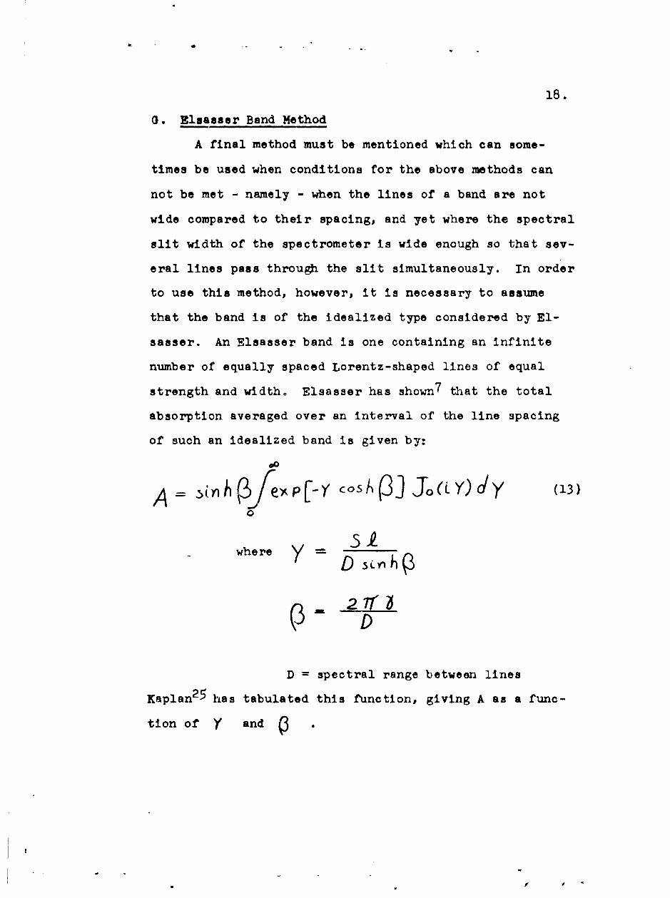
G. Elsasser Band Method

A final method must be mentioned which can some-

times be used when conditions for the above methods can

not be met - namely - when the lines of a band are not

wide compared to their spacing, and yet where the spectral

slit width of the spectrometer is wide enough so that sev-

eral lines pass through the slit simultaneously. In order

to use this method, however, it is necessary to assume

that the band is of the idealized type considered by El-

sasser. An Elsasser band is one containing an infinite

number of equally spaced Lorentz-shaped lines of equal

strength and width. Elsasser has shown7 that the total

absorption averaged over an interval of the line spacing

of such an idealized band is given by:

A --.= , 5( e P [-Y' cos,('3.] Jo(i Y)cly (13)0

where D

D = spectral range between lines

Kaplan 2 5 has tabulated this function, giving A as a func-

tion of Y and

19.

III EXPERIMNTAL DISCUSSION

A. Spectrometer

It is well recognized that the princil barrier

to obtaining spectra with high resolving power in the

thermal detection infrared liss in the difficulty in get-

tfrg a sufficiently high signal/noise ratio with narrow

slits. In 1950, the Laboratory of Astrophysics and

Physical Meteorology of The Johns Fopkins University

began the design* of a spectrometer transmitting a large

light flux -- sufficient to enable the use of much higher

resolution than was possible before. The construction

of this spectrometer has been completed, and its perform-

ance tested, The instrument has demonstrated 26 an optical

slit width of 0.06 cm-1 at 600 cm "1 , which is only 15%

greater than the theoretical width. In addition a wave-

length accuracy of 0.01 cm-1 at 600 cm-1 has been achieved.

The essential features of this spectrometer are described

below:

(1) Optics

Figure 5 shows scleratically the optics of the in-

strument. It is of the Ebert type,27 the Ebert mirror

being 30' in diameter and of 90' focal length. The grat-

ing is 14" wide and 12N high ruled 1000 lines to the inch.

*The principles upon which this design was based were de-scribed by John Strong in a paper discussing high resolv-ing power in the infrared, presented at the 1950 meetingof the Ohio State Symposium on Molecular Structure andSpeo troscop~yo

20.

The slits are 3 " long and are curved on a 15" diameter

circle. Either a Globar or a carbon arc2 8 ' 2 9 can be used 4

as a source. In the present work a Globar was used. The

light is chopped at the source with a mica chopper, travels

through the Ebert system, and coming through the long exit

slit it is sliced and condensed onto a Golay cell pneu-

matic detector. Figure 6 shows the operation of the image

slicer. In effect, it slices the 3" long exit slit into

three 1" long segments, and causes these segments to be

imaged adjacent to one another on the detector. A similar

arrangement is used with the carbon arc on the entrance

side of the spectrometer to enable the crater of the car-

bon arc to fill the long entrance slit.

The elimination of overlapping grating orders is

effected by 3 or 4 reflections of the light from MgO crys-

tals in conjunction with the mica chopper. Since the

0.003" thick mica chopper transmits well out to 9 microns

and only the a c. co-ponent of the signal incident on the

detector is amplified, higher order light is considerably

reduced. Figure 7 shows the reststrahlen reflection from

a typical MgO crystal. After four such reflections, the

first order of the grating from 14 to 25 microns is ob-

tained completely free of higher order light even when a

carbon arc is used.

(2) Grating

The 141 x 12" grating was ruled in a 13-micron

thick silver film evaporated on a glass blank with

21.

excellent uniformity using a new technique30 which was

developed here. The ruling was done by Dr. H. W. Babcock

on the large ruling engine of Mt. Wilson and Palomar Ob-

servatories.

Before the ruling of the large blank, many small

gratings were ruled in similar silver films by Mr. Wilbur

Perry of the Johns Hopkins Gratings Laboratory. These

gratings, all blazed for the 20-micron region, were ruled

with different groove forms and their blazes studied, in

order to determine the optimum specifications for the

groove of the large grating.

Figure 8 shows some of the data taken for a small

grating having a groove form similar to that specified

for the large grating. The specifications decided upon

were a groove spacing of 25 microns and a facet angle of

250. These specifications have the effect of shifting

the maximum of the curve in Figure 8 to somewhat longer

wavelengths.

Figure 9 is a photograph of the grating in its mount-

ing on a table, adjustable with respect to its axis of

rotation. The detailed reflection indicates the sharpness

of the blaze.

(3) Drive and Rotation

Figure 10 is a closeup photograph showing the drive

mechanism incorporated to rotate the grating. The screw

adapted for the drive of this spectrometer was originally

made to test new mothcds of making ruling engine screwa. 3 7

n vt- --

22.

It is driven in fixed bearings so that the nut moves when

the screw is rotated. A sapphire flat mounted on the

moving nut pushes on a steel ball fixed at the end of

the grating table azm to cause the rotation. This type

of drive yields a cosine variation in angular velocity

of grating rotation which just compensates for the cosine

dependence of grating dispersion. As a result, when the

screw is driven by a synchronous motor, the variation of

wavelength on the exit slit of the spectrometer is remark-

ably linear in time0

The rotation axis of the grating is located by four

highest precision Fafnir ball bearings. These bearings

are mounted in pairs spaced two feet apart. The pairs

are made up of matched bearings arranged so that the

errors in one are compensated by those of the other.

The pairs are proloaded by a small force directed along

the axis of rotation. This force eliminates any bearing

"slop."

(4) Alignment Instrument

To obtain the maximum available resolution from the

spectrometer, critical alignmont of its components is

necessary. Figure 11 shows the schematic operation, and

Figure 12 is a photograph of an instrument devised which

greatly facilitates the alignment of the spectrometer.

Its operation is describea in the caption for Figure 11.

(5) C02 and H20 Removal

The spectral region of operation of this spectrometer

23.

contains strong atmospheric CO2 and H20 absorption. Thus,

if these gases are to be studied under controlled con-

4 ditions, or if other gases are to be studied with which

the C02 or H20 interfere, the residual CO2 and H20 must

be removed from the spectrometer. In the present case

one would expect this tobe a particularly difficult task

since high resolution is available, and the optical path

of the spectrometer is about 15 meters. However the

following procedure was remarkably successful.

The spectrometer is completely enclosed in a copper

housing, and can be operated entirely from withcut. All

wires to the interior run through hermetic seals, and a

copper-lined door can be sealed into place during opera-

tion. The C02 is removed from the interior atmosphere by

circulating the air through KOH pellets. After 4 to 6

hours, a desiccant is added to the path of circulation by

remote control. The highly effective desiccant used is

Linde Air Products Molecular Sieve. Several more hours

of continued circulation removes all trace of the CO2 and

H20 from the spectrometer path. Figure 13 demonstrates

the success, showing the complete disappearance of the

C02 fundamental Q branch, and the double H20 line at

592 cm- l, which affords the strongest H20 absorption

between 15 and 19 microns.

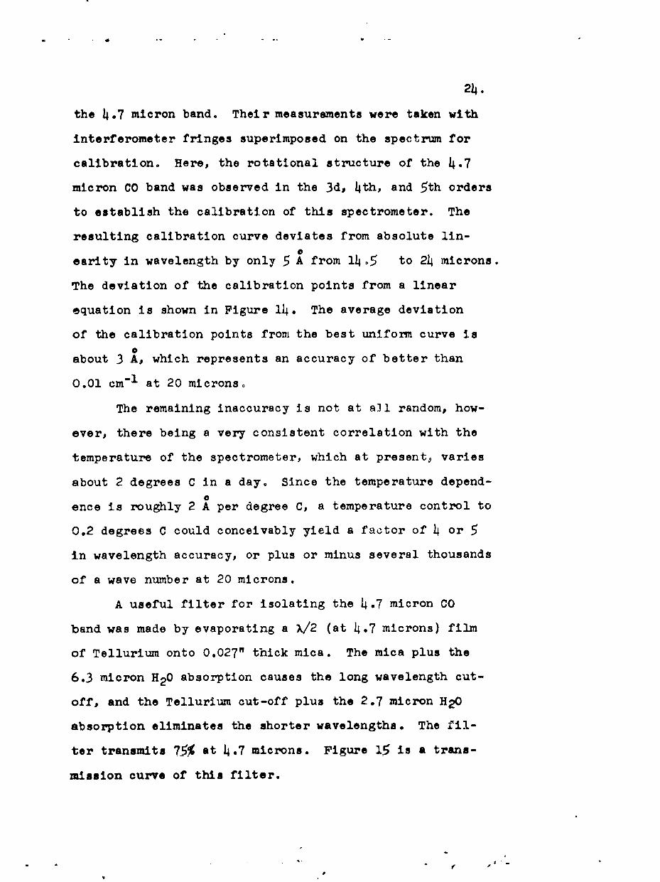
(6) Calibration

The spectrometer was calibrated using the wavelength

determinations of Plyler, Blaine* and Conner 3 1 on CO in

24.

the 4.7 micron band. Their measurements were taken with

interferometer fringes superimposed on the spectrum for

calibration. Here, the rotational structure of the 4.7

micron CO band was observed in the 3d, 4th, and 5th orders

to establish the calibration of this spectrometer. The

resulting calibration curve deviates from absolute lin-

earity in wavelength by only 5 A from 14.5 to 24 microns.

The deviation of the calibration points from a linear

equation is shown in Figure 14. The average deviation

of the calibration points from the best uniform curve is0

about 3 A, which represents an accuracy of better than

0.01 cm-1 at 20 microns.

The remaining inaccuracy is not at all random, how-

ever, there being a very consistent correlation with the

temperature of the spectrometer, which at presento varies

about 2 degrees C in a day. Since the temperature depend-0

ence is roughly 2 A per degree C, a temperature control to

0.2 degrees C could conceivably yield a factor of 4 or 5

in wavelength accuracy, or plus or minus several thousands

of a wave number at 20 microns.

A useful filter for isolating the 4.7 micron CO

band was made by evaporating a X/2 (at 4.7 microns) film

of Tellurium onto 0.027" thick mica. The mica plus the

6.3 micron H20 absorption causes the long wavelength cut-

off, and the Tellurium cut-off plus the 2.7 micron H 20

absorption eliminates the shorter wavelengths. The fil-

ter transmits 75% at 4.7 microns. Figure 15 is a trans-

mission curve of this filter.

25.

(7) Resolution

The available resolution of the instrument was

determined by observing the widths of absorption lines

of N20 in the 17-micron band. The spectrometer slits

were set equal to the theoretical Rayleigh resolution

limit as calculated for the 14" wide grating and W = 17

microns. The carbon arc was used as a source to supply

the maximum possible signal/noise ratio. N20 at 35 mm

pressure was introduced to a 25 cm absorption cell.

Figure 16 shows the R(4) and R(5 ) lines of the N20

17-micron band with hot band satellite lines completely

resolved 0.2 cm- 1 away. The observed width of absorption

of the lines is about 0.08 cm- 1 . Under these conditions,

the e2fectivo optical slit wldth of the spectrometer would

be about 0.06 cm- 1 . The broader appearance is due to the

influence of the width of absorption of the line itself --

as would be observed with infinite resolution. This rep-

resents 70% of theoretical resolution for the grating

used at the angle corresponding to 17 microns, which com-

pares favorably with 80% calculated theoretically by Jac-

qutnot 3 2 for the use of slits equal to the diffraction

width.

As can bei seen from Figure 16, the signal/noise

ratio is just about the minimum necessary to do effective

work, and so it would appear that this spectrometer has

reached the diffraction limit to resolution and the energy

limit to resolution simultaneously.

- - '4 - - ,i

44

26.

(8) Electronics

The electrical signal generated by the Golay pneu-

matic detector is amplified with an a.c. amplifier. The

amplified signal is rectified synchronously with the

chopping frequency by a mechanical rectifier, after which

it is fed through an RC filter network with an adjustable

time constant. The signal is then displayed on a Leeds

and Northrup pen recorder.

B. Experimental Set-Up for the Study of C02

The first problem to which the spectrometer, de-

scribed above, has been turned is the present study of

the C02 intensities in the 5b5 - 667 cm-1 spectral region.

For this work the Globar was used as a source. The entire

3" of slit was used in conjunction with the exit slit

image slicer. The slit width used for all measurements

was 0.24 mm, and corresponds to an optical slit width of

about 0.1 cm- 1

Three absorption cells, of lengths 1.133, 5.08, and

25.17 cm were constructed to fit into the exit beam of the

spectrometer. (From here on these cells will be referred

to as the 1, 5, and 25 cm cells.) The cells were made of

brass and had KBr windows. The windows were sealed by

means of neoprene o-ring seals. The absorption cell in

use was connected to the exterior of the spectrometer

housing by copper tubing so that the gas content could be

controlled from the outside. A one-liter glass bottle

was connected to the system on the outside as a ballast

4!

27.

volume, which was especially useful in maintaining a con-

stant pressure over a long period of time when the 1 cm

cell was being used. Two Hg manometers were used to read

the pressure in the absorption cell. The entire system

to be isolated was of metal or glass, except for the o-

ring seals at the cell windows and the connections to the

copper tubing -- which were of plastic hose. The system

could be isolated for many hours with no detectable change

in pressure. The cells were filled to a prescribed pres-

sure with pure C02. The brand used was blue banded South-

em Oxygen Co. CC2 , and the purity of this brand has been

checked in the past to be better than 99.7%°

A constant check of the temperature of the absorp-

tion cell was kept by reading the voltage of a thermo-

couple attached to the absorption cell.

For all runs the spectrometer housing was sealed up

and all CO2 and H20 were removed froTL the spectrometer path

before beginning any measurements. From the recorder a

record was obtained of the gas transmission as a function

of wavelength for several pressures in each cell. Repeats

were often made.

The wave number locations of the C02 absorption

lines of interest in this study were taken from the work

of Blau, etco, 3 and appear in the tables. The use of

their accurate measurements avoids the necessity of deal-

ing with the temperature dependent error of this spectrom-

eter [see A(6)J.

28.

The amplifier was quite stable and maintained a

steady zero signal over many hours. The 100% transmission

curve was checked at frequent intervals by recording the

signal after pumping out the absorption cell. The amount

of scattered radiation could be determined by observing

the depth of absorption for the strong C branches, and in

most cases unwanted radiation was negligible. A small

scattering correction was introduced in the region below

618 cm-1 .

29.

IV. DATA

A. Spectra

CO2 absorption spectra were observed from 545 to

674 cm"1 under a variety of pressures in each of the 1,

5, and 25 cm absorption cells. It is impractical to in-

clude all this data here. The tables include the results

from all measurements, but only representative spectra

are shown. Figures 17 and 18 are spectra of the entire

range of study in these experiments, using the 25 cm

absorption cell with the pressures indicated. Each vibra-

tional transition is indicated at the band head, and the

P and R branch lines are labeled according to the J quan-

tum number of the lower state and the following convention:

for C120J 6 Aa : R,P branch 0l'0 - 000

B,b : " 0220 01'0

C,c : 0200 - 01'0

K,k : "C'O - 0200

Ff: " 03'0 - 0220

for C1301 6 " 01'0 - 0002

The spectra shown here were taken with a spectral

slit width of , 0.1 cm 1 , which is the highest resolu-

tion with which the CO2 spectrum in this region has ever

been recorded. Thus more lines are visible and a better

identification of satellites is possible than heretofore.

Figure 19 is a scan of the 0l'0 - 000 q branch with

higher dispersion. The Q branch line positions are marked.

30.

The frequencies of the clearly observed Q branch lines

together with the constant (B"-B') they define are given

in Table 3o

From Figures 17 and 18 it is obvious that a con-

siderable portion of the spectral range is crowded to the

extent that measurements on individual lines would be dif-

ficult. Therefore measurements were not made on all lines.

Three regions were selected for concentrated study: 661 -

666 cm- I , 624 o5 - 629 cm- 1 , and 598 - 613 cm-1. These

regions were selected for the following reasons. a) The

principal lines in these regions 4iie nearly free from over-

lap; b) lines of low, medium, and high J occur; and c) the

strength of the lines occurring in this region allow con-

venient-sized absorption cells to be used.

Spectra in the first region, 661 - 666 cm l.. are

shown in Figure 20 with high dispersion. A scan with each

of the l 5, and 25 cm absorption cells is represented.

Lines a2p a4, and a8 of the V2 fundamental P branch were

studied, as well as lines b8 and b9 of the ist harmonic

P branch. Also an estimate was made of the strength of

the 018 C12016 isotope fundamental Q branch,

Spectra occurring in the second region of study

624.5 - 629 cm- 1 are shown in Figure 21p with scans using

the l, 5, and 25 cm absorption cells. The lines studied

here were a50, 52, 54, and 56 of the fundamental, and

C9, 11, and 13 of the R branch of the 0200 - 01'0 transi-

tion. The third series, of "apparent lines in Figure 21

31.

are blends of k and oe, lines and therefore not suitable

for an intensity study.

In these bands alternate J lines are missing. This

is because in each transition a _ state is involved,

which for CO2 contains only levels of even J.*

The third region of detailed study was 598 - 613 cm- I

as shown in Figure 22. Here P branch lines c7 through

c25 of the 0200 - 01'0 band are found quite free from

overlap or background. (The F band lines occurring here

have only a two or threo percent contribution which may

be easily taken into account.) For this reason the most

accurate measurements were made in this region.

In addition to a concentrated study in these three

spectral regions, a measurement of the total Q branch

strength was made for the 0200 - Ol'O band at 618 cm- I,

the 03'0 - 0220 band at 597 cm -, and the 03'0 - 100 band

at 544.5 cm-1l

The Q branches for the 03'0 - 0200 band and the fund-

amental of the C1 3016 and 018Cl201 6 isotopes are nearlyI2hidden under P branch lines of the C1 2016 fundamental (see

2Figure 17). However, rough estimGtes were possible of the

strengths of these bands. Figure 23 shows the spectral

region 646 - 649 cm"1 taken with lower pressure in the

25 cm absorption cell where the 03'0 - 0200 band of C120J 6

and the 01'0 - 000 band of C1 301 6 occur. The 01 8C12 01 62

*The oxygen nuclei being identical and of zero spin, theantianmetric (odd J) levels of states are absent.

32.

fundamental Q branch can be seen with high dispersion

in Figure 20.

B. Analysis of the Spectra

The methods used to determine the line widths and

strengths from the observed spectra are described in

Section II. In the case of the P branch lines of the C

band it was possible to use several methods, and the re-

sults c.,ald be cross-checked. The most frequently used

method is the "Curve of Growth" method described in Sec-

tion II-Eo A further remark is made here with regard to

the application of this method to the present study.

The important result of the "Curve of Growth" treat-

ment is stated in Equation 110 To repeat,

0 / Z 'ff(f (11)

If the value of WO for a line is known at two absorption

path lengths, SO and 6 can be calculated for that

line. This procedure is cumbersome, however, since F(x)

is in tabular form. Instead of this, a graphical pro-

cedure has been used which yields results more readily.

This is as follows- The data are plotted as log W ver-

sus log a . A curve of log F versus log x is then

superimposed on the data curve and positioned so that

the best fit is made with the experimental points0 (These

curves are most conveniently obtained by the use of log log

graph paper.) A simple argument then shows that S° is

equal to the value of WO at the intersection of the

33.

Ladenburg-Reiche curve "linear region" asymptote (F() =)

and the line log 2=O ( - 1 cm). Further, it may be

shown that the value of WO at the intersection of the

"linear region" asymptote and the "square root region"

asymptote (F(x) .amv) is given by WO = 4 60. Thus

S0 and 60 may be determined quite simply when ihe data

are put in this graphical form.

In the discussion to follow concerning the reduction

of the data, the three spectral regions in which a con-

centrated effort was made will be considered in turn,

followed by a discussion of the treatment of the various

Q branches observed.

(1) 661 - 666 cm-1 Region

The lines occurring in the first region of interest,

661 - 666 cm - 1 , are strong, and low pressures are required

to eliminate overlap and keep down the background. As a

result the lines are narrower than the optical slit width

and direct measurements are impractical even with slit

function corrections. Also, the lines are too strong to

use the "Weak Absorption" method. Therefore the "Curve of

Growth" technique was attempted for the analysis of this

region. The average WO of a2, 4, 8 determined from sev-

eral runs at various pressures for each of the 1, 5, and

25 cm cells is given in Table 4. The pressures used for

each cell length are indicated in Table 5. The data were

plotted graphically as discussed above. Figure 24 shows

the result for the line a4. As can be seen from the

34.

grapn, the experimental points fit the logarithmic

Ladenburg-Reiche curve (abbreviated L-R curve in fur-

ther discussion) almost entirely in the "square-root"

region. Therefore the data can not yield SO and 6 0

with any accuracy, but will determine the product SO 30

to the accuracy of the measurements. For the "square-

root" region it has been stated in II-E that

v =2 Y53. (8)

or -2V3T (16)

In a region close to the "square-root" region, a better

approximation is: 0-2 b5 (0 a 0(7)

Since x is necessarily large for this approximation, a

rough value of x is all that is required. The S 3'

products were determined for a2, a4, and a8 for each WO.

These results are shown in Table 8.

The value of WO for the lines b8 and b9 was deter-

mined from the spectra taken with the 25 cm absorption

cell. Equation 17 was used to determine S 60 for b8 and

b9. If the assumption is made that b for b8 and b9 is

equal to 60 for a8, the ratio of S0 for b8 and b9 to

SO for a8 may be determined. In a similar manner, the

strength of b34 plus b35 (see Figure 17) was determined

35,

relative to the strength of a34. These results are tabu-

Alated in Table 9. (In Table 9, the strength of b34 + b35

is divided into a contribution from each line assuming a

Boltzmann distribution. )

The strength of the Q branch of the 018C12016 band

was estimated using the "Elsasser band" method. A de-

scription of this case will be included in a later dis-

cussion of several Q branch strength determinations by

this method.

(2) 624.5 - 629 cm- I Region

The second region studied, from 624o5 to 629 cm- ,1

contains many closely spaced lines. P branch lines of

the A, K, and Ar bands and R branch lines of the C band

occur predominantly. Also P branch lines of the B band

and R branch lines of the F band occur weakly. This region

is of interest since it is the only region in which measure-

ments on R bianch lines of the C band and high J lines of

the A band can be attempted0

The equivalent widths of a50, 52, 54, 56 and C9, 11,

13, were measured at various pressures (Table 5)p and an

average WO calculated for each line for each absorption

cell length. These are shown in Table 4. The measure-

ment of equivalent width of a line requires that an inte-

gration be made over all absorption due to the line. It

can be seen in Figure 21 that the absorption due to each

line is overlapped by that due to others for the 1 cm

path length measurements. This difficulty may be overcome

Of

36.

by a simple approximation which holds well when the over-

lap absorption is small and the lines do not differ greatly

in peak absorption. First the absorption is divided into

regions by drawing vertical lines between the absorption

lines, dividing their spacing into components of length

having the same ratio as their peak absorption. The

equivalent width of a line is then measured by integrat-

ing the absorption over the block containing the line.

The assumption is that the integrated absorption lost

by cutting off the wings of the line being measured is

compensated for by including the wings of the neighboring

lines when the cutoff is made in the manner prescribed

above.

It was necessary to make background corrections to

the WO values for the a50, 52, 54, 56 lines. A theoret-

ical spectrum was calculated using values of band strength

and line width that have been estimated by Benedict.3 4

The contribution of the background lines to the equivalent

width measured was then calculated for each condition of

pressure and path length used. The appropriate correc-

tions were made to the observations. These corrections,

averaging only a few percent and the largest of which is

8% have been used on the values of WO occurring in Table 4.

Due to the weak absorption, and overlap and back-

ground corrections necessary, the values of WO for lines

in this region obtained with the 1 and 5 cm path lengths

have considerable uncertainty. To increase the accuracy

37.

obtained by the graphical "Curve of Growth" method, the

data for a50, 52p 54, and 56 were plotted together for a

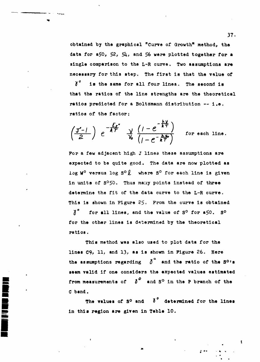
single comparison to the L-R curve. Two assumptions are

necessary for this step. The first is that the value of

ao is the same for all four lines. The second is

that the ratios of the line strengths are the theoretical

ratios predicted for a Boltzmann distribution -- i.e.

ratios of the factor:

( 2 (I-"e) for each line.

For a few adjacent high J lines these assumptions are

expected to be quite good. The data are now plotted as

log WO versus log S°2 where S0 for each line is given

in units of sO50o Thus many points instead of three

determine the fit of the data curve to the L-R curve.

This is shown in Figure 25. From the curve is obtained

a0 for all lines, and the value of SO for a50. so

for the other lines is determined by the theoretical

ratios.

This method was also used to plot data for the

lines C9, 11, and 13, as is shown in Figure 26. Here

the assumptions regarding 6' and the ratio of the SO' s

seem valid if one considers the expected values estimated

__from measurements of 60 and S° in the P branch of the

3....C band.

The values of S0 and 0 determined for the lines

in this region are given in Table 10.

i

38.

(3) 598 - 613 cm-1 Region

The only strong lines in this region are the c7 -

c25 lines of the 0200 - 011 0 band P branch. Here pres-

sures up to an atmosphere do not cause serious overlap,

and SO and 60 were determined for these lines by

direct measurement as well as by the "Curve of Growth"

method.

Direct measurements were possible with only small

slit function corrections, since the width of the absorp-

tion coefficient curve at a pressr.re of 1 atmosphere is

over twice the width of the spec .meter slit function.

The logarithm of the transmission curve was calculated for

4 ruhs with the 1 cm and 5 cm absorption cells where

the pressure was between 0.8 atmos, and 1.0 atmos. Then

obs. was measured directly, and SO was obtainedobs.

by integration of the log T curve for each line -- as dis-

cussc.d in II-B. These observed values were corrected for

the effect of the slit by the amounts indicated in Fig-

ures 1, 2, and 3. The resulting 80 and o for each

line is given in Table 6.

The equivalent width of each line c7 - c25 was

measured for the lo 5, and 25 cm path lengths for sev-

eral runs under a vdriety of pressures -- as indicated

in Table 5. The value of W0 for each line at each path

length j given in Table 4., These values of WO were

smoothed by plotting WO versus J for each path length

and drawing a smooth curve through the experimental

39.

points. This is shown ir Figure 27. Log W° (smoothed)

was plotted against log g , and SO and 60 for each

line determined by the graphical "Curve of Growth" method.

An average example of the fit of the data to the L-R

curve is shown for line c17 in Figure 28. The resulting0

values of SO and 6 are given in Table 6 where they may

be compared with the results of the corrected direct

measurements.

(4) Q Branch Measurements

The Q branch strength of six bands was determined.

In the discussion below, they will be grouped According

to the method used to reduce the data.

The Q branch of the 0310 - 100 band at 514.26 cm - 1

is weak and is free from overlap with other bands. The

"Weak Absorption" method was used to determine the strength

of this Q branch. The integrated absorption was averaged

for four scans over the Q branch, and the strength deter-

mined as outlined in II-D. The value obtained is given in

Table 11.

The Q branch strength of the 0200 - 01'0 transition

(C band) and the 0310 - 0220 transition (F band) were

determined by the method of Wilson and Wells. For each

band, f(-(nT)v was evaluated at several conditions

of path length ind pressure (see Table 7), and S0 deter-

mined by the extrapolation procedure outlined in II-F.

For the C band Q branch the strength of the Q branch +

line cl was determined, since this first P line is well

, .~ -

I409

surrounded by Q branch structure. After a minor back-

ground correction for overlapping "a" and " C " lines.,

the C band strength was determined from the measured SO

by the ratio of the C Q branch + cl line to total band

strength calculated assuming a Boltzmann distribution in

the P branch. The extrapolation is shown in Figure 30,

and the C Q branch strength is included in Table VN 11.

The F band Q branch measurement was a much more

approxim te procedure. Before the method of Wilson and

Wells could be applied, the effect of the line c27 had

to be removed from the absorption due to the F q branch.

This was done by carefully reconstructing the c27 line as

it would appear in the absence of the F Q branch. It was

assumed that the absorption due to c27 was equal to the

average value of absorption for the lines c25 and c29

which could be clearly observed. After constructing the

c27 line the difference between the constructed and ob-

served absorption was assumed to be due to the F Q branch,

and the method of Wilson and Wells was pursued. The extrap-

olation for the F Q branch strength is shown in Figure 29.

The resulting Q branch strength is included in Table 11.

The remaining three Q branches are nearly buried

beneath P branch lines of the A band, and are also over-

lapped with lines of the B and C band3. An accurate de-

termination of their strengths cannot be made by direct

meaaurements; however a rough value was obtained using

the following technique: First an estimate was made of

41.

the absorption due to the Q branch as a function of v.

From the band constants, separations of the Q branch

lines were calculated at frequency inteivals greater

than the spectrometer alit function width. The "Elsaseer

Band" method, II-G, was then applied for each frequency

at which the line separation was calculated. From Equa-

tion 13 the SO of the average strength line being passed

by the spectrometer when set at that frequency was deter-

mined. A a' of 0.11 cm-1 was assumed for the calcula-

tion. For each of the line strengths thus determined, a

Q branch strength may be calculated if a Boltzmann dis-

tribution is assumed for the Q branch, The Q branch

strengths for the K band and the isotopic 4 band were

determined in this manner, and the results are given in

Table 11. The Q branch strength of the 01'0 - 000 transi-

tion of the 018 C12 016 isotope was also estimated by this

method. This Q branch has two series of lines as a result

of f -doubling. Since the even J series diverges more

rapidly, it makes the major contribution to the absorption

in the wing of the Q branch. The measurements were made

in the wing of the Q branch, and the effect of the odd J

series was ignored in the reduction, The contribution to

the observed strength due to this second series is esti-

mated roughly as 30%. Making this correction to the ob-

served 50, the value of Q branch strength found in Table 11

represents a "most probable" choice.

42.

V. DISCUSSION OF RESULTS

The primary results of this study are the values of

SO and 60 determined for the lines listed in Table 10,

and the Q branch strengths listed in Table 11. An esti-

mate of the uncertainty in these results is listed for

each value in the table -- the most important source of

uncertainty being the lack of reproducibility of the

quantities derived directly from the spectra due to the

noise fluctuations.

The band strength determinations are considered

secondary results since an assumed band intensity distri-

bution must be used in the calculation of these quantities.

In the discussion below, the results of this study

are compared with the results of other experimental and

theoretical investigations. A discussion of strengths

will be given first, followed by a discussion of line

widths .

A. Line and Band Strengths

The line strengths for the P branch of the C band

obtained from the corrected direct determination and the

"Curve of Growth" methods are plotted as a function of J

in Figure 31. This curve establishes the experimental

variation of strength with J. In a first attempt to com-

pare these results with theory, the rotational distribu-

tion was calculated assuming a Boltzmann distribution.

It has been shown33 ' 11 that this distribution for CO2

a0

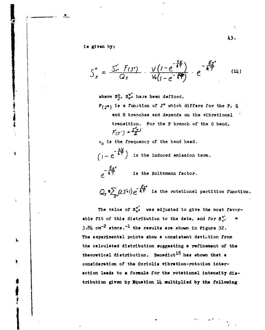
43.

is given by:

§ - S F(J') (1e-1

where SO, Svo hare been defined,

F(t ) is a fun.,tion of J" which differs for the ,o

and R branches and depends on the vibrational

transition. For the P branch of the C band,

F(j")Vo is the frequency of the band head.

(i- 4) is the induced emission term.

k is the Boltzmann factor.

QT 11ZJ4)e ' is the rotational partition function.

The value of Svo was adjusted to give the most favor-a V1

able fit of this distribution to the data, and for S.

3.84 cm-2 atmos.-l the results are shown in Figure 32.

L The experimental points show a consistent deviution from

the calculated distribution suggesting a refinement of the

theoretical distribution. Benedict1 8 has shown that a

consideration of the Coriolis vibration-rotation inter-

action leads to a formula for the rotational intensity dis-

*tribution given by Xquation 14m ultiplied by the following

4

44.term.-

I( 2 (15)

-4- where m is the ordinal numbeir of the line, and 5 is a

parameter depending on the strength of the Coriolis inter-

action and the vibrational transition invulved. No thec-

retical estimates have been made of the value of for

the C band, although = +.0016 has been estimated 18

for the A band.

Using Equation 14 with the addition of the term (15)

and adjusting the parameters S40 and . a most satis-

factory fit to the experimental data is obtained. Thisis shown in Figure 33 for Sl = 4.27 cm-2 atmoso- and

= +.0035.

The effect of a positive is to decrease the

intensity of the P branch and increase the intensity of

-on. the R branch. The parameters were adjusted so that almost

perfect agreement with experiment is obtained at ell --

--- the value of SO for ell being 0.0685 cm- 2 atmoso-l . For

the R branch, the predicted value of SO for C11 is

0.0736 cm- 2 atmoso- I while the experimental value is

0.070 cm- 2 atmoso-l . This agreement is well within the

estimate of reliability for the measurement of SO for C1l.

The determination of S*# for the C band from the

C q branch measurement must be considered as a check on

the value obtained from the other measurements. The value

obtained in Svc 3.72 cm- 2 atmos.- 1 which is 13% lower

45.

than the value determined above from the P branch measure-

ments. The uncertainty in the value obtained from the Q

branch measurement io considerably greater than that for

the determination from the P branch measurements however,

due to the abundance of data in the latter case. It should

also be mentioned that a consideration of the effects due

to the Fermi resonance between the 0200 state (upper state

for the C band), and the 100 state yields the conclusion

that the observed strength of the C q branch should give

too low a value of Sv' if the effects are neglected, as

they were here. The magnitude of this effect, however,

has been estimated3 4 as less than 5%0

The distribution of line strengths in the funda-

mental, or A, band can not b6 determined from measure-

ments made in this study since the strength has been

determined at only one place in the band. If a distri-

bution is assumed however, the band strength can be deter-

mined from the measurement of the line strengths for a50 -

a56 given in Table 10. The distribution assumed is that

given in Equation 14 multiplied by the Coriolis term (15),

where / for the P branch of the A band. This

calculation has been carried out for three values of

q . -O corresponding to no Coriolis inter-

action; + +.0016 which is the value calculated1 8

theoretically for this band; and + +.0035 which in

the value obtained in this study for the 0 band. Bene-

dict points out34 that the magnitude of the parameter

° -t** - 4

46.

for the C band is expected to be somewhat greater than

that of the A band. For these three values of , the

values of S v , for the L band are:

V/

SVW (cm"2 atmos.-l)

0 196

+ .0016 235

* .0035 290

The result of Kaplan and Eggers1 6 measurement on

the v2 fundamental by a low resolution "Curve of Growth"

V/method is S v A = 214 cm- 2 atmoso-l. The strength of

a50 observed in this study can be obtained from their

value of SYN if a of .00084 is assumed. No finalV'conclusion can be drawn as to the value of Sv. for the

A band, but in light of all available evidence, the most

reasonable value is perhaps 235 cm"2 atmos. "I with a

= +.0016.

The strength of the first harmonic, or B band has

only been determined relative to the A band, and is

therefore equally ambiguous.

Vibrational transition moments were calculated by

Equation 1 for all the bands studied. The results appear

in Table 12 where they are compared with the transition

moments that have been calculated by Benedict1 8 on the

basis of a theoretical model. The available parameters

in the dipole expansion for this model have been adjusted

to beat fit the C02 intensity data known previous to the

47.

present study, and no attempt was made to further adjust

the parameters in light of the present results. Three

values of transition moment havo been calculated for the

A and B bands corresponding to a value of for the

A band of 0, +.0016 and +.0035.

The agreement of other investigations (740 - 864 cm"1

region) with the predictions of the model is included for

comparison.

B. Line-Widths

The values of 3 o for c7 - c25 determined from

corrected direct measurements and the "Curve of Growth"

method are included in Table 6. In addition 50 values

have been determined from "square-root region" measure-

ments of SO in the 25 cm cell and from th6 bedt values

of line strength determined by all methods. The results

of these three methods of obtaining b are shown graph-

ically in Figure 34. Included also is the value of 60

obtained from Kinetic Theory assuming a collision diam-

eter, d = 3.3 x 10- 8 cm, given by viscosity and conduc-

tivity measurements.* 50 has the almost constant value

of 0.103 cm- 1 from c9 to c23. There is a slight indica-

tion of higher values of o at lower J" and lower values

at higher J". The o determined from R branch measure-

ments on C9, 11, 13 has the value 0.11 cm-1 .

jO was determined for the P branch of the funda-

mental (A band) to be a = 0.060 cm-l at a50 - 56.

The value of to for a2, 4. 8 could be determined from

tandbook of Chemistry and Physics, 30th edition, 2627(1947), Chemical Rubber Publishing Co., Cleveland

, @

i48.the SO 1 products of Table 8 if the band strength and

intensity distribution were known. Three values of A

band strength were calculated in the previous section

for 0 = , +.0016, and +.0035. The values of 60

for a2, 4, and 8 calculated from the SO 3o products

for these three cases are:Se6(a2) (4) a(a8)

cm'2atm', cm-latm -I cm-latm-1 cm-la~p-i

0 196 .129 .116 .095 - 10%uncertainty

+.0016 235 .108 .098 .08 in allvalues

+.0035 290 .088 °079 065

For any reasonable choice of it would appear

that the 30 at low J" is considerably higher than the

o at J" 50. This result fits well with the observed

trend of 6 versti J" in the C band. It is proposed

therefore that in the A and C bands of C02, o is high

at low J, beqomes nearly constant at a somewhat lower

value over intermediate J, and drops off at higher J to

approach the Kinetic Theory value. This propEition is

quite compatible with theoretical expectation. It has

been shown3 5 '3 6 that molecules with a strong dipole moment

have a maximum value of 30 at a J" value near the peak

of the Boltzmann distribution, since a molecule making a

transition at such a J" finds a greater number of perturb-

ing molecules with PiAch it may resonate. However this

effect is very weak for molecules with a small dipole

moment. Smith, Lackner, and Volkov3 6 have measured 6o

49.

for OCS in the microwave region and measure only a 7%

increase in So from J" = 1 to J" = 5. They have also

calculated the expected widths using Anderson's Theory 3 5

of collision broadening extended to include the effects

of near-resonant interactions and conclude that the ex-

pected increase in 65 is only 4% from J" = 1 to J" 5

for OCS.

CO is another molecule with a weak dipole which has

been investigated. Measurements of 6 for the CO funda-

mental have been reported by Benedict o18 The results,

reproduced graphically in Figure 35, show a variation with J

not inconsistent with the results of this study for C02.

The observed increase in o at low J can be explained

by the following argument: In the case of a very weak

dipole-dipole interaction, or for a quadrupole-quadrupole

interaction (which must be the principal cause of colli-

sion diameters greater than the Kinetic Theory diameter

in a non-polar molecule such as C02 )0 the collisions in

which exact resonance occur are relatively less important

than those in which a moderate degree of near-resonance

takes place. Since the low J levels are more closely

spaced, a molecule radiating from a low J quantum state

will have significant near-resonant collisions with a

greater number of molecules, causing an increased line

width.

VI. CONCLUSIONS

The distribution of line strength and the variation

of line width with : has been determined for intermediate

0 0

50.

J in the P branch of the 0200 - 01'0 absorption band of

CO2 . The observed intensity distribution can be com-

pletely explained if the Coriolis vibration-rotation

interaction is introduced. The line width is quite con-

stant from J" = 9 to J" = 23, with some indication of

being larger for lower J and smaller for higher J. The

strength and line width of the J50 to 56 lines in the P

branch of the 01'0 - 000 band have been measured; however,

the band intensity is indeterminate since the magnitude of

the Cor4.olis interaction parameter is not known for this

band. A value has been obtained for the strength of all

the absorption bands of C02 prominent at room temperature

in the spectral region 545 - 667 cm I ... with varying

reliability.

It is suggested that measurements be made with long

absorption paths on higher J lines in the P branch of the

0200 - 0l'0 band to determine the further variation of

line width with J.. and to establish th( val.ue of the Crnri-

olis interaction parameter with greater certainty. It Is

suggested also, that a further study of the low J lines

in the Ol'O - 000 band be made with shorter path lengths,

to determine the strengths of these lines -- for in this

way the magnitude of the Coriolis interaction parameter

for this band could be established, the band strength

determined, and a comparison of line widtbsbe made for

low and high J.

BIBLI OGFAPHY

1. L. D. Kaplan, Jour. Chem. Phys. 18, 186 (1950)

2. S. S. Penner, Jour. Appl. Phys. 23, 1283 (1952)

3. Blau, Dalby, Lakshmi, Nielsen, Rao, Infrared Spec-

troscopy of Molecules, Contract DA-33-019-ORD-1507,

Ohio State University (1955)

4. To appear in Table of Solar Spectrum Wavelengths,

2.8 - 23 Microns, by Migeotte, Neven and Swansson,

Proc. of Royal Society of Ligge

5. R. Ladenburg and F. Reiche, Annalen der Physik 421,

181 (1911)

6. E. B. Wilson, Jr. and A. J. Wellsp Jour. Chem. Physo

,, 578 (1-946)

7. W. M. Elsasser, Physo Rev. 2, 126 (1938)

8. P. Martin and E. F, Barker, Physo Rev. 4!, 291 (1932)

9. A. M. Thorndike, Jour. Chem. Phys. 13, 868 (1947)

10. H. Rcbens and E. Ladenburgs Verhod.D. Physo Ges. 7,

179 (1905)

ii° D. F, Eggers. Jr. and B. L. Crawford, Jr., Jour. Chem.

Phys. 19, 1554 (1951)

12. Howard, Burch, and Williams, Near Infrared Transmission

Through Synthetic Atmospheres, Report No. 1, Con-

tract AF19(604)-516, Ohio State University (195 )

13. W. Peters, Dissertation, The Johns Hopkins University

(19149)

14. W. H. Cloud, The 15 Micron Band of C02, Progress Report

Contract Tnr 2148(01), 'he Johns Hopkins University

(1952)

15. H. J. Kostkowski, Dissertation, The Johns Hopkins

University (1955)

16. L. D. Kaplan and D. F. Eggers, Jr., Intensity and

Line-Width of the 15 Micron C02 Band Determined

by a Curve of Growth Method, presented at Ohio

State Symposium on Mol. Struct. and Spectros. (1955)

17. L. D. Kaplano Jour. Chem. Physo 15, 809 (1947)

18. W. S. Benedict, Theoretical Studies of Infrared Spectra

of Atmospheric Gases, Final Report, Contract No.

AF19(604)-i001, (1956)

19. A. Adel, Physo Rev. 52, 53 (1953)

20. W. S. Benedict and S. Silverman, Line Shapes in the

Infrared, paper given at Meeting of Am, Phys. Soc.,

(January 154)

21. H. A. Lorentz, Proc Roy. Acad. (Ams o) 8, 591 (1906)

22. H. J. Kostkowsk! and A. M. Bass, Slit Function Effects

in the Direct Measurement of Line Widths and Intensi-

ties, presented before the Opt. Soc. of Am. (October

1955)

23. P. C. von Plants, private communication

24. L. H. Stover, Table to be published as part of a paper

by L. D. Kaplan and D. F. Eggers, entitled Intensity

and Line-Width of the 15 Micron C02 Band Determined

by a Curve-of-Growth Method

25. L. D. Kaplan, Jour. of Meteorology 10, 100-104 (1953)

26. R. P. Madden, A High Resolution Spectrometer for the

20 Micron Region, paper presented at the Ohio State

Symposium on ol. Struct. and Spectros. (June 1956)

27. W. G. Fastie, Jour. Opt. Soc. Am. L, 641 (1952)

28. C. S. Rupert and J. Strong, Jour. Opt. Soc. Am. 40,

455 (1950)

29. J. H. Taylor, Dissertation, The Johns Hopkins Univer-

sity (1952)

30. R. P. Madden, 10-15 Micron Thick Silver Films for

Infrared Gratings, paper presented before the

Opt. Soc. of Am. (March 1955)

31. Plyler, Blaine, and Conner, Jour. Opt, Soco Am. 5, 102

(1955)

32. P. Jacquinot, private communication

33. B. L. Crawford, Jr. and H. L. Dinsmore, Jour. Chem.

Phys. 18, 983 (1950)

34. W. S. Benedict, private communication

35. P. W. Anderson, Phys. Rev. 76, 647 (1949)

36. W. V. Smith, H. A. Lackner, A. B. Volkov, Jour. Chem.

Phys. 23, 389 (1955)

37. J. Strong, Jour. Opt. Soo. Am. 41, 3 (1951)

I r

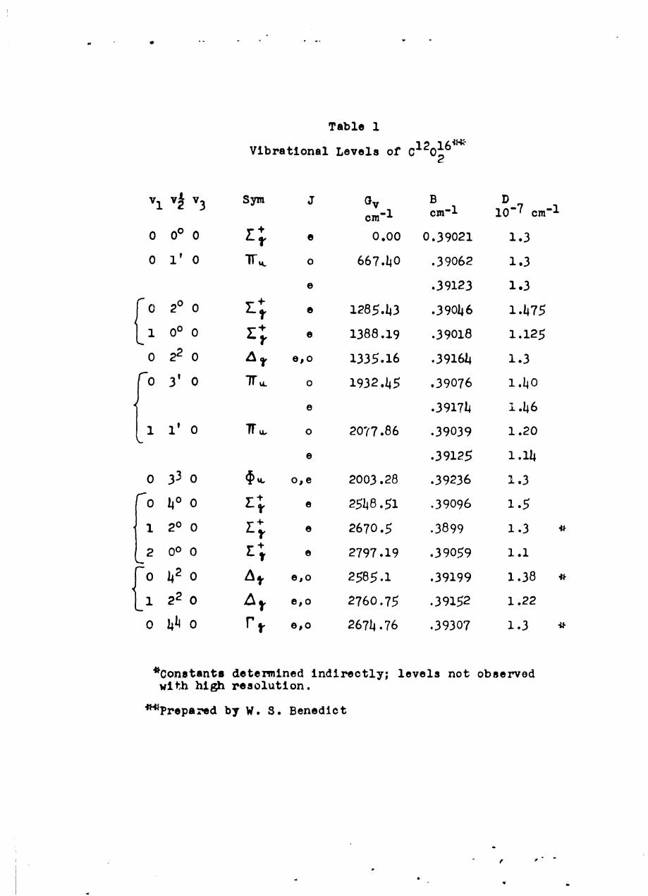
Table 1

Vibrational Levels of C120161

2

vI vv v 3 Sym J Gv B D

cm-1 cmI1 10-7 cm-1

0 00 0 a 0.00 0.39021 1.3

0 1' 0 - o 667.40 .39062 1.3

e .39123 1.30 +0 2 0 t 1285.43 .39046 1.475

0 0 e 1388.19 .39018 1.125

0 22 0 e,0 1335.16 .39164 1.3

0 3' 0 r o 1932.45 .39076 1.40

e .39174 1.46L : ' 0 T o, 2077.86 .39039 1.20

e .39125 1.14

0 33 0 U. o,e 2003.28 .39236 1.3

0 40 0 Z: e 2548.51 .39096 1.5

1 2 0 e 2670.5 .3899 1.3 *

2 00 0 + e 2797.19 .39059 1.1

0 42 0 At e,o 2585.1 .39199 1.38 *

1 22 0 e,o 2760.75 .39152 1.22

0 44 0 r eo 2674.76 .39307 1.3

*Constants determined indirectly; levels not observed

with high resolution.

"Prepared by W. S. Benedict

0

I

r-~r 0o N~ N N

0000

m I CUHHI

0o co I8C 0O

T 1 0 cy r-4 r-a, (V N N

00

1-3 a 0 0O 0 0 H 0

0 . %D 0l rn N 00vgui N 0 H O '

0 , H, a, %0) a a ,N ~ ~ A-D %0 % 0 w *

0

E-4 *P I,) 0 0 0 0 0 0 0

0(n (n Aj e (n N C i00 00 0

00 HN

431 00 COJ I

0

Table 3

Line Positions and Band Constants

Determined for the Q Branch of the

0110 - 000 Transition of C212

Line v Observed*cm-1

Q38 668.91

40 669.07

42 669.27

514 670.46

56 670.68

These line positions have been fitted by the

following equation:

v = 667.140 + (B'-B")J(J+l) + (D'-D")j2 (j+l)2

The resulting band constants are:

B-"= (10.17 + .1o) x io-4 cm-1

DID"= ( .32 + .30) x 10-8 cm-1

*These frequencies were determined relative to the

position of R branch lines J" 2.4 as determined

by Blasa, etc*3

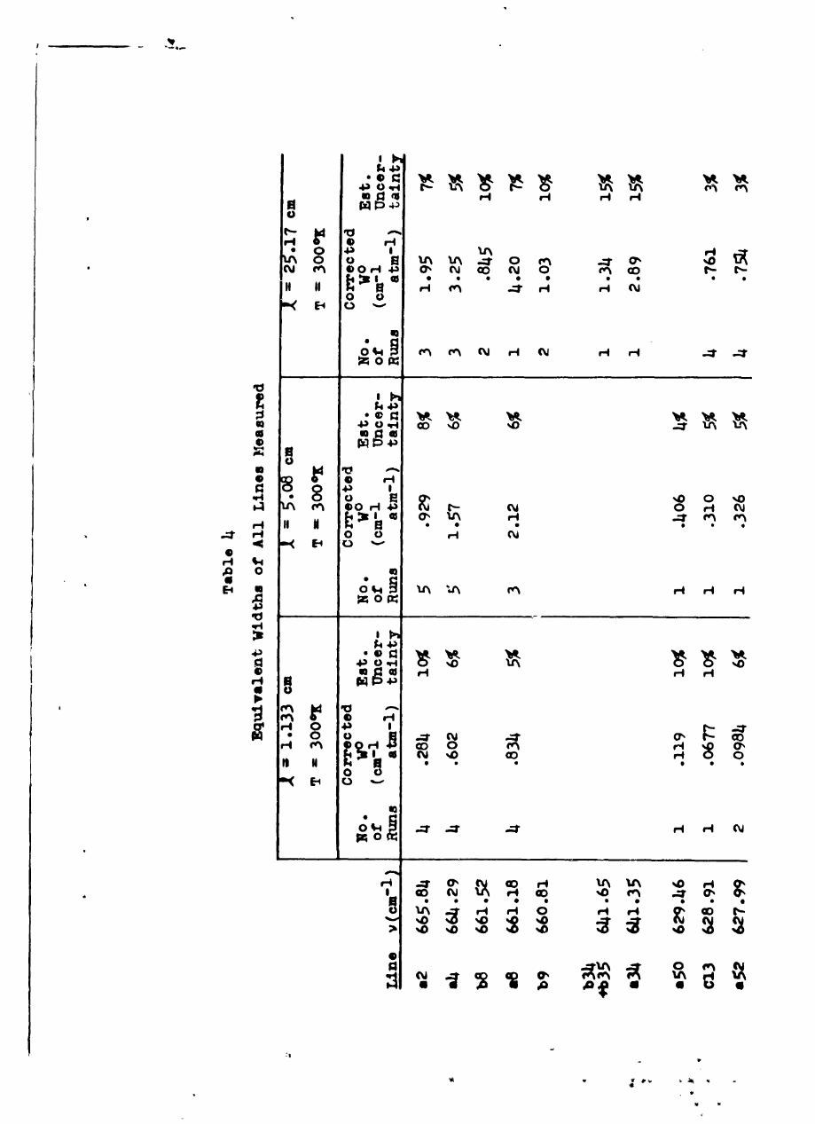
~zl43

0 4~ k vt 'Lk Ht %k0 0 "A t- V\ m M

0A 0

E4 H

0E-44

0 A0

43 W4 C() "D~ 0

H0 1%NFeSS 000 0

0

UH H- H-

4. 0 H t H

H 0 43

* 00 0 a, Ca

vi -- -

toC

'LA 5 0 0 0 0 0 0

..0 1 H H 4

%V Z8 %

%0 %a %0

C,4

-4 C. 1 10

0 4- H t- --

F 4 S.) i

0 W20

o o coH-

43 1

0)

lrN- a) '--- '- r-l H r-4 Oj N Cj Cj N N N CQ N (V

43

CCO--' 0 ) aD 0- V\~ '.n C'D 0: ' C', mI -,o aD~0 4~0 N ~ N N N Nn _ N N N N

t cIC 0 * * 0 0 0 0 0 0 *

00

0C0

4-) ~~ H GoX 0 N _Z t-0 m % m 00V.4 I M IA OD.0 IA o A -- G 0 00' -'0 x

0 O U a 0 ~ ~ ~ H p .

~30 0 000 0 00 0 0oD No % 0Uo % 0 %

00 Nr NI N- N% Hv r-4 r-f r- r-4 cu rY N'

Table 5Pressures and Path Lengths Used in Study of CO2

P (atmom)4 1.133 5.08 _25.17 4- .t~m)

.198 1

.13 1

.129 1

__ .06 1

.1322 1

.0658 1

.0255 1

.99 2

.197 2

.068 2

.053 2

.997 3

1.00 3

.790 3

1.00 3

.285 .3

.198 3

Region 1: 661 - 666 cm "1

2: 624.5 - 629 om'I

" 3: 598 - 613 cm 1

B

IU

I-

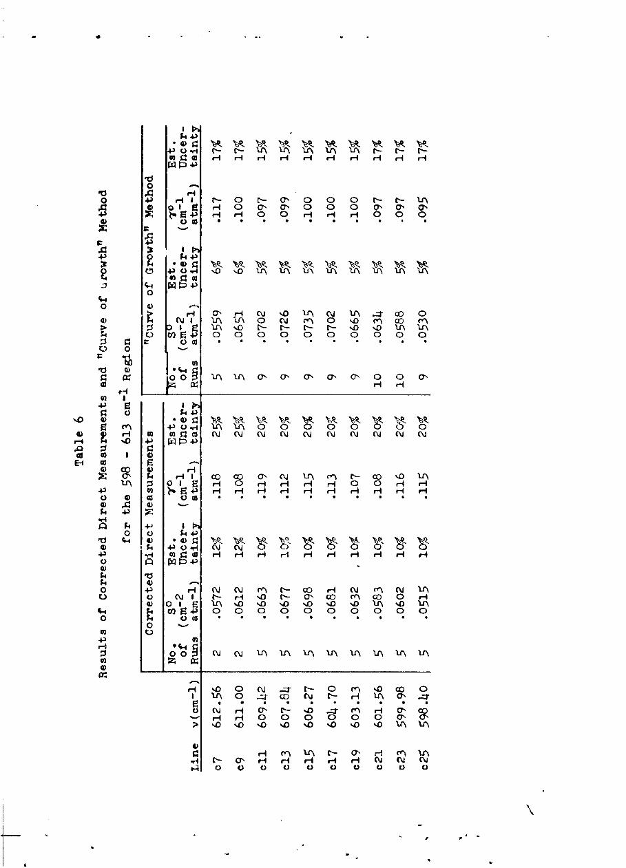
-P C -H (I C - in - -

@0 H H H- Hi H H H H H H

0o 43 H-4I r- 0 C- c'. 0 0 0 C-- t-- %A'

4) 0I HO rI a, 0- 0 0 0 a7' a, a'%P 0 -P H H o 0 H H H 00 0

U Io

0

0H a' H N %.0 bJ-\ N~ 'lF\ _: G 00

C) 0

0 H H

@2 I4-) C)0-

'0 0 \. 44-) 0 r4j IA V 0 0 00 0 ~0

4) ~ ~ ~ w to 0N1 ~ ~ ~ N N N~ N~ N N~

E-4 0C 0

r- a HI co aj ON N tC\ cvn C- Go '0 J0I HO4r. H Hl H- H 0 0 H. H

-P @ im4-) H- H- H- H- H- H H- H- H- H-

0) QL 44

0- 4) o0!$4 4 -*)~ -ri P \Is sQ.

43 * m2 0 H- Hl Hl H H H- H H H- H-

44>

0 4P H- N~ N~ m~ t-- co H- N~ (V) N\ LlfsO 0 N~jI t- H- -I0 C- cr' 0) en c 0 H-

0- 00I 0 ' 0 0 0 9 0 9 9

0om2 0

4.3@H

004 N~ IA 'LA'\ 1 La )\ tJ C L

H D 0 ON Zr Cl-- m~ G oV\~ 0 _- co N C-H IA a'N

a N H; a' r-: '.0 .z HH Ho 0 0 0 0 0 a '

Ph 0 %. . .0 '0 0 %D0 %0 VL\ %LA

.4

t4 0 Q 0Q )C )C

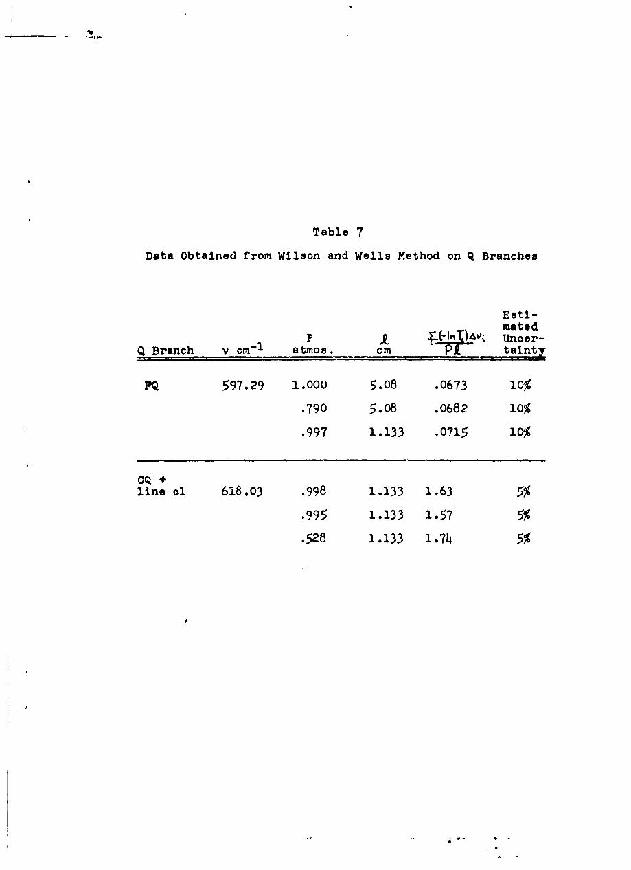
Table 7

Data Obtained from Wilson and Wells Method on Q Branches

Esti-mated

PV IV% T)~iv Uncer-Q Branch v cm- I atmos. cm PT tainty

FQ 597.29 1.000 5.08 .0673 10%

.790 5.08 .0682 10%

.997 1.133 .0715 10%

CQ +

line cl 618.03 .998 1.133 1.63 5%

.995 1.133 1.57 5%

.528 1.133 1.74 5%

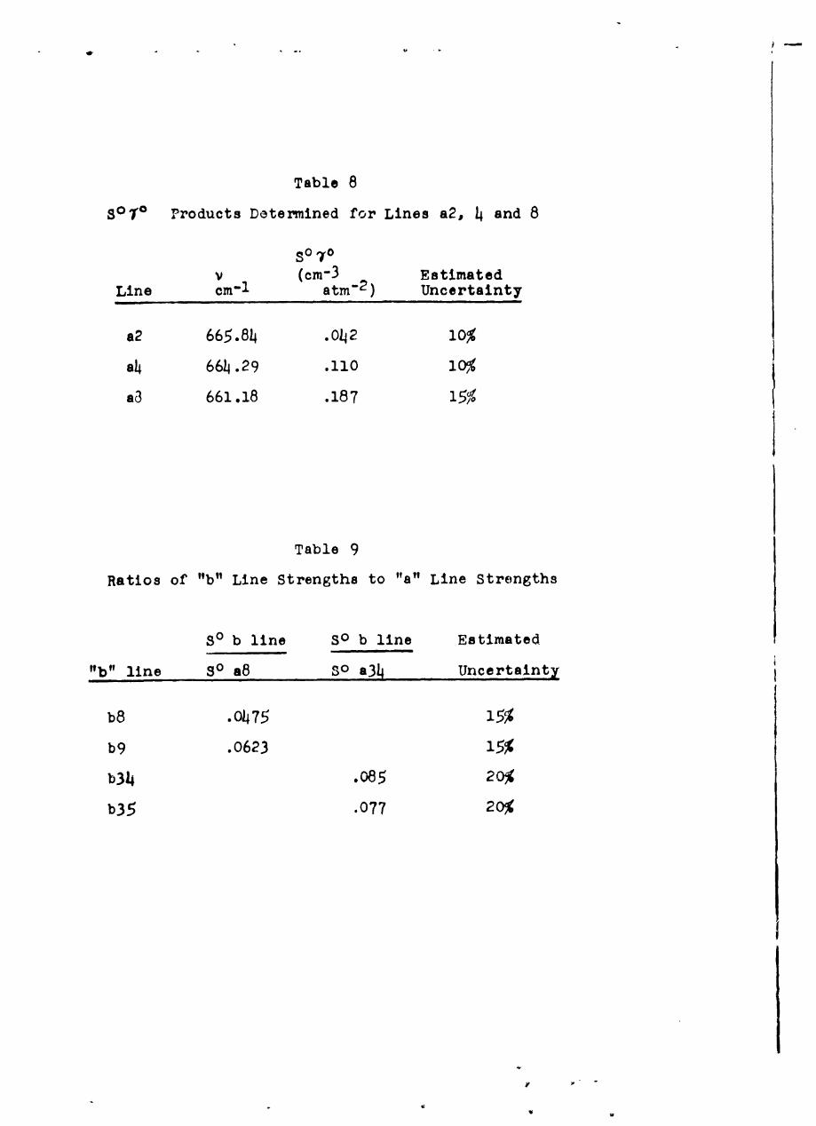
Table 8

SOTO Products Determined for Lines a2, 4 and 8

Soov (cr-3 Estimated

Line cm-I atm "2 ) Uncertainty

a2 665.84 .042 10%

a4 664.29 .110 10%

a3 661.18 .187 15%

Table 9

Ratios of "b" Line Strengths to "a" Line Strengths

SO b line SO b line Estimated

"b" line so a8 SO a34 Uncertainty

b8 .0475 15%

b9 .0623 15%

b34 .085 20%

b35 .077 20%

Table 10

SO and -/0 for Individual Lines Determined in this Study

SO in Est. of 1o in Est. ofcm- 2 rtm-1 Uncer- cm-latm 1 Uncer-

Line v(cm "1 ) at 300*K tainty at 300K tainty

a50 629.46 .143 7% .06 9%

C13 628.91 .0750 7% .11 9%

&52 627.99 .101 7% .06 9%

CIlI 627.38 .0695 7% .11 9%

a54 626.51 .0704 7% .06 9%

C9 625.83 .0613 7% .11 9%

a56 625.05 .0481 7% .06 9%

c7 612.56 .0565 3% .111 15%

c9 611.00 .0627 3% .108 15%

cll 609 .42 .0682 3% .105 12%

c13 607.84 .0712 3% .lo 10%

c15 606.27 .0715 3% .103 10%

c17 604.70 .0692 3% .103 10%

c19 603.13 .0656 3% .103 10%

c21 601.56 .o614 3% .102 10%

c23 599.98 .0568 3% .101 12%

c25 598.40 .0522 3% .099 15%

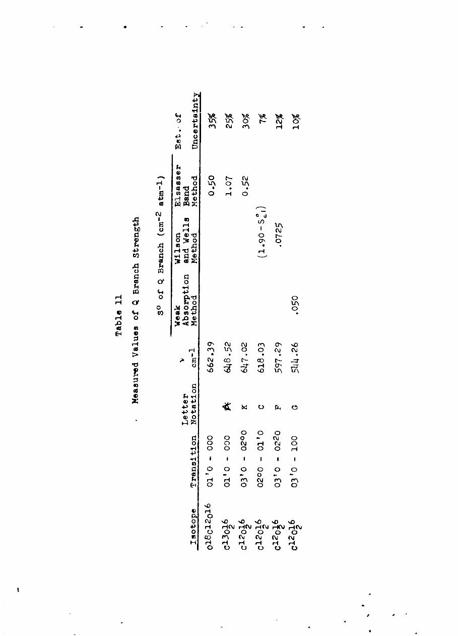
t- N

I)1too 0 o0 %-, 0) t-

H :3t 0 crA 00L

4. o20 0 Hd 0

4. 04)

0 r o 0

0) 0~3 U' 0

0 Ix010

0 004

49.

H H (nr 00 ~ ~> I 0

N 0c (1- 00 r- ')

E-4 0r

0 0

0 0

o. 0 C) ~

-ri 00 0 0 4

S0 0 0 0 0 0~40 00 0 Hr I I- in*j n t

E- 0 0 0 0 0 0

0 N - % 0 -D -0

H. H r-4\ rC% N HN e'N04 0 0 0 0 0 0

V) HD f\ V

H H- H H H H H0 U) C) C) C. 0

40

V 43 * :3 0%O0* ( '

0'4H 0 - F- (Vw

434

HP fu r- 0 %0 a-f %2~ 0 -T~)H '0 CO '- D e 0 H co N 0', Nu Go

*44. H Nj N H NV m enNC 0 H- cm

430 4i *- *l- en %D ID 142HH0IN e

,0IHI

"4.9.4 0

3 10 e(n 0N ON -IrI

0C~ 4- 0 0v ~ -

E 1 IO Z 0 -:r a% -1 %D .4 H4 Nz

H H U -H j N N

H H 0d V_

4. %) 0 U' XA %D A -4

W4 4-40 0 0 $410 0 4 0 4 1010 0 0 0 0 0 0 00 00 00

> +4- '

0D C7% 0 V % 0 NQ 0"oH (V C 0 Nv I^

I) ~ ~ ~ ~ ~ ~ ~ - %D-g w o - s - -.. '0

%'0 %00

4-10 40

43 -P Ci 0 PZ Q0* 04-3

0 0 0 0 0OH0 N 0 00 04-4 0 3HH s N NO 0 0

a 0 0 0 0 H 0 0

0 0 0 00 00 000 N -

04 00 000 00

4103 0 V)

0~ CU " n O

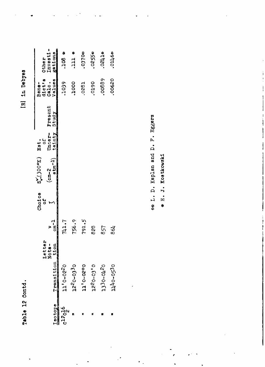
N .40 U) 0 c 4 C4) O 4) -18 4 N N H-

A Pl-43 H H 0 0 04'3 go 0 0

a] 0" 0'

@2 0 *4) 0' 0 H- 0 co N04O 0 e 0 W~ 01 CC) %0~UHH 0 0 N H 0 0SW-4 (d0 H H 0 0 0 0

43

3

4a~ 0 CO

@2 l0

S H ca

0~ 50 4' z

P4 soT> o s0

-H-

H El ON U\

r- H '0 H 00 C-- _:T~U ~ t( 0'N U\ '%D

0 0 V

4) 0 41

o 0 0 0 0 0 04-j M~ N --IA

.-H 0 0 0 0 0 00) 1 1 1 1 1 1

* 0 0 0 0 0 0

4.' 0' H N H N .0.

* 0 HN

HO

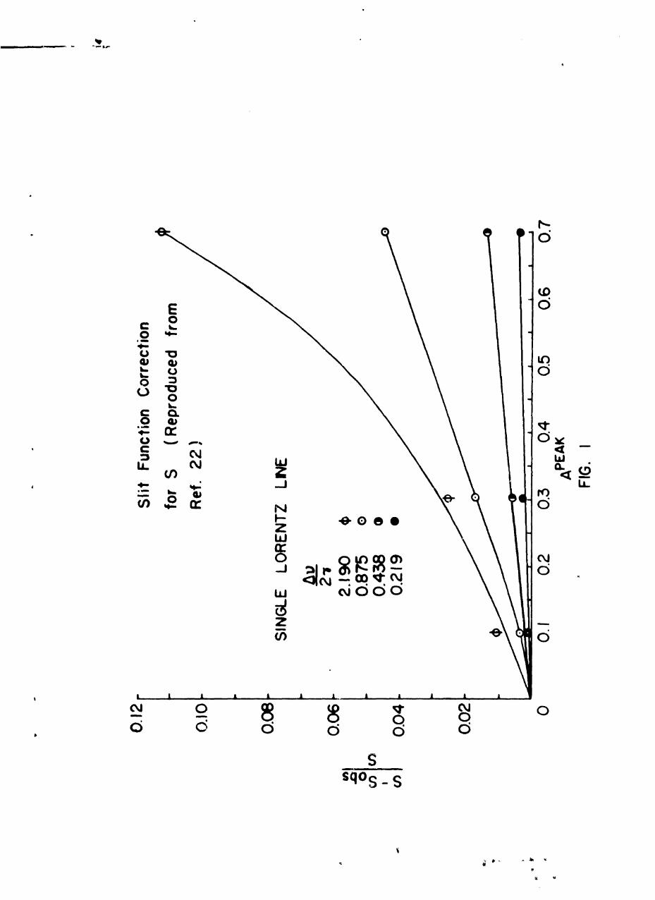
.00

((0

00

00h.le

00

05d

s4Nqo LUL

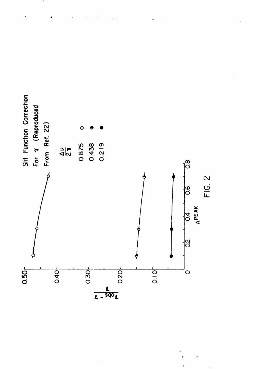
CN

0 o1

0 LL

E w~cM

c- b- 0

L -L

sqoL~

00

0

0w4)

CW~

.2a

W or

: ..

0 0

0 e 0 ~

lV3dV

)QV3d Vd

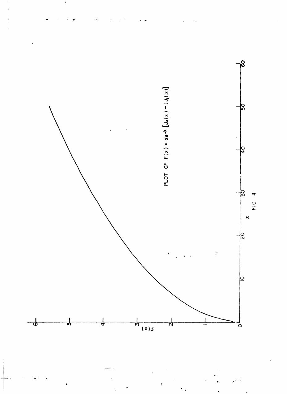
00

0~

.10

-5-0

C~

in In Xyj CK

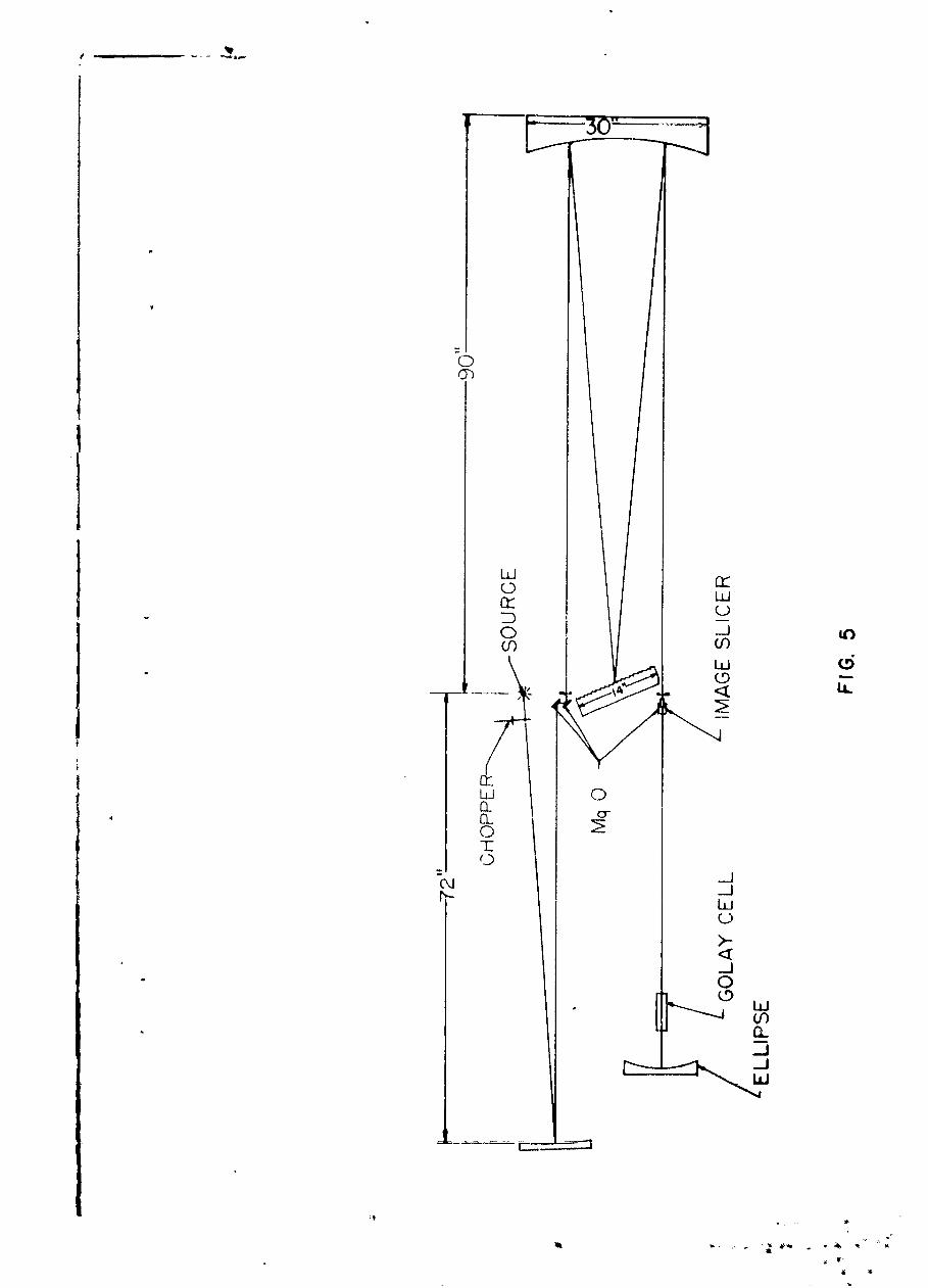
o -1t

r Li.

~j

00 U)L

C-

Li

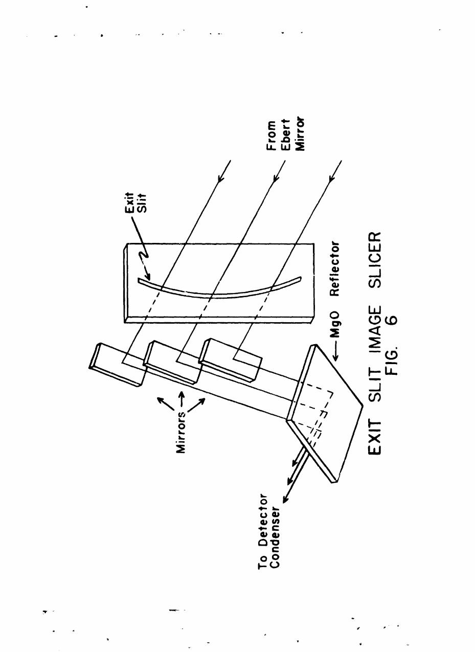
U- w

0 u

4-C-

.z (00

00

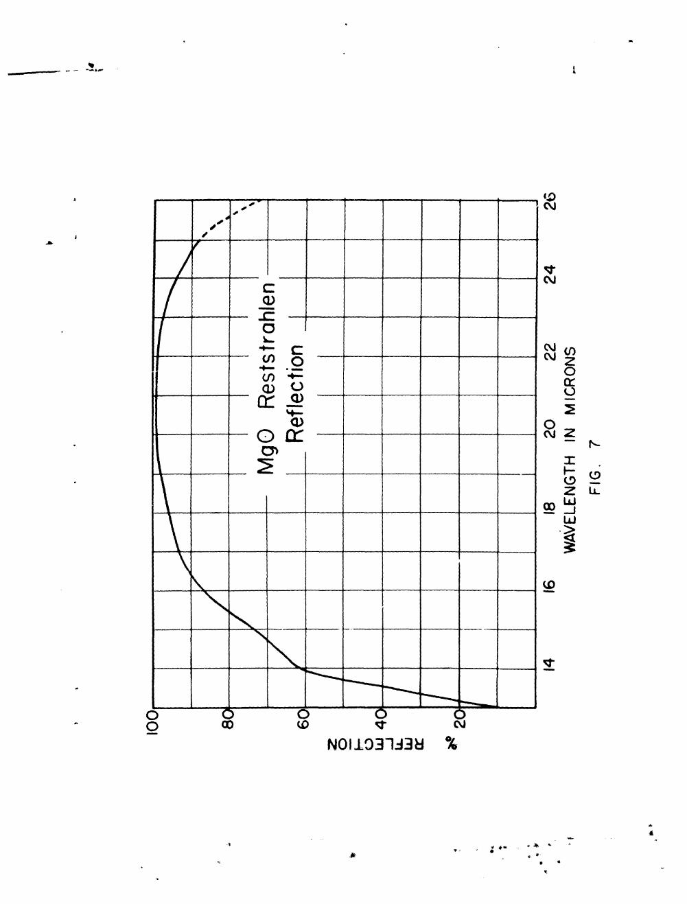
a~~ - - -

CP

__ -'-- __ NV

(0z 0_ __ DO c

OD __ 0

N0104-3

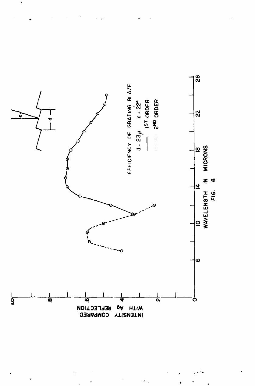
wN

CID cr c(DN LiM

(A) 00~

0

OD-U

z z

U-J

(0

A-i

rw

C4.

.....

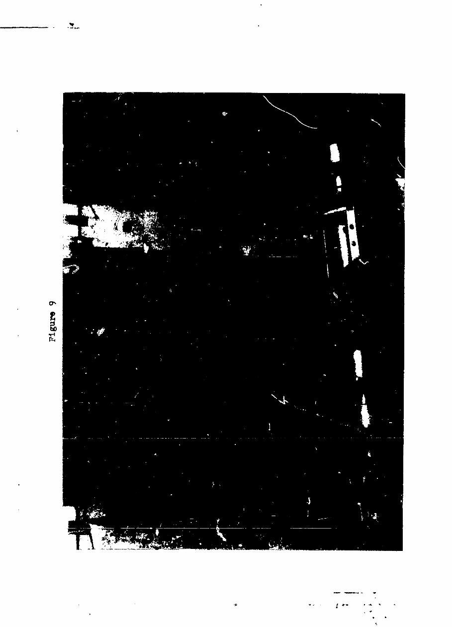
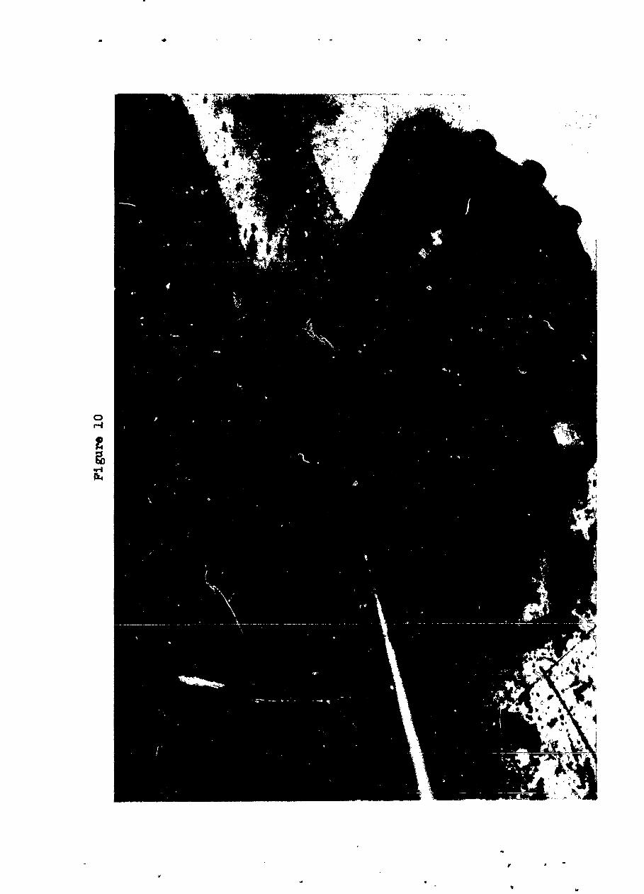
4i

0i

Caption for Fiure 11

This instrument is used to facilitate the

alignment of the Ebert system as follows:

A plane mirror with a central hole is mounted

on a hollow cylinder. An eight-point suspension

restricts this cylinder to rotational freedom alone.

(The bearings are indicated in Figure 11 by "cross"

marks.) As a preliminary step the plane mirror is

made perpendicular (by autocollimation) to the axis

of rotation of the cylinder and the instrument is

then positioned in the Ebert optical system as shown

in the figure. Cross hairs mounted inside the cyl-

inder are illuminated from the side arm, and, when

viewed as indicated in Figure 11, the planes of the

object and image cross hairs are brought into co-

incidence by moving the cross hairs forward or back

from the Ebert mirror until they lie in the focal

plane of the Ebert mirror. The rotation axis of the

alignment instrument is then made parallel to the

optic axis of the Ebert mirror by adjusting either

the Ebert mirror or the position of the alignment

instrument until there is no relative iotion between

the cross hairs and their image when the cylinder is

rotated. A microscope mounted on an arm fixed to the

cylinder may then be used to critically adjust the

position, curvature and focus of the slit jaws.

*w

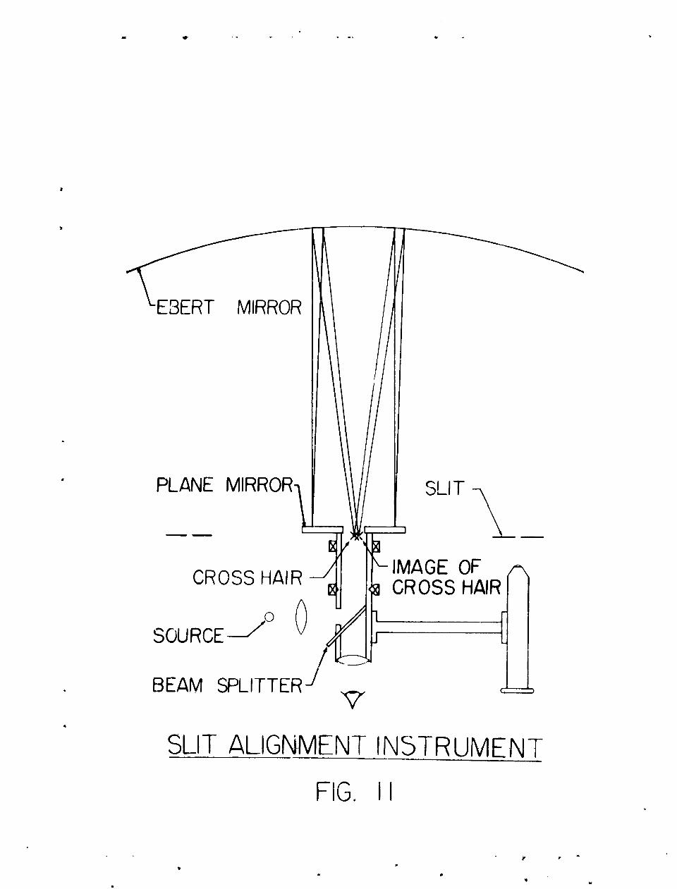
= 41, °- -. - -

E3ERT MIRROR

*PLANE MIRROR SLIT

7r

CROSS HAIR IMAGE OFCCROSS HAIR

SOURCE--/D 4

BEAM SPLITTER LI

SLIT ALIGNMENT INSTRUMENT

FIG. II

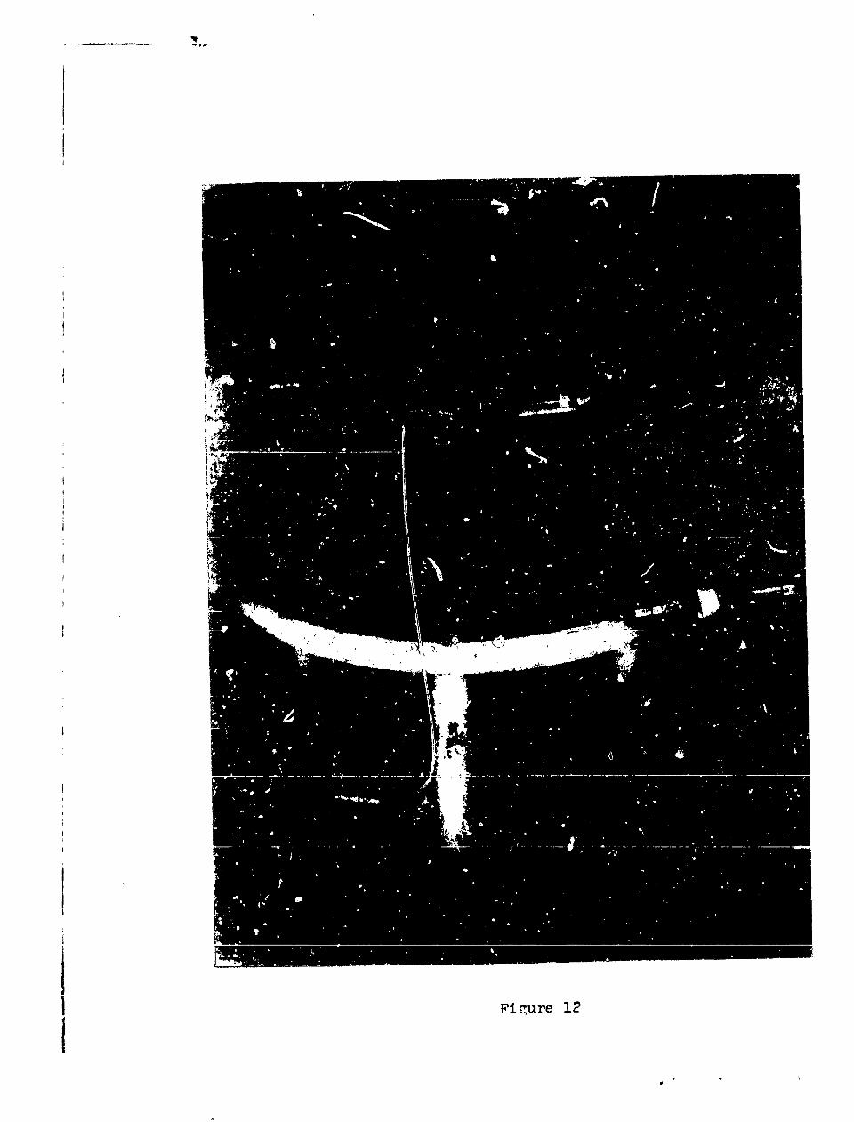
I~F Fhure 1

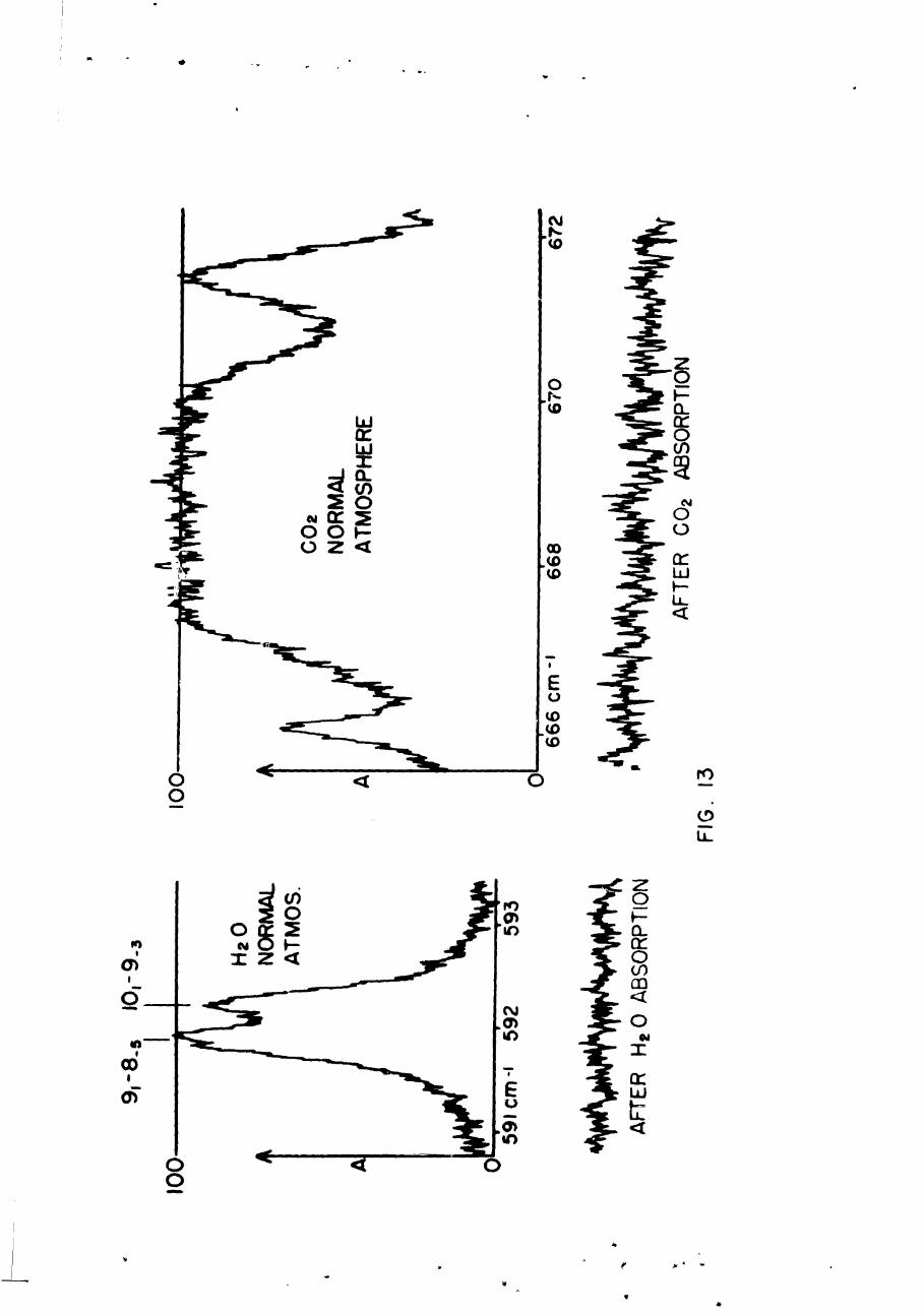
0r 0

a.:0 : 0

0 z 00

00

LL-

z (0

(00

tz0t

50 /9M

oil

UU

W >

0I +

U-) N -j

UW

iczl

in %*0 OD*

CY~

*N

C~w V N 0 C OD+ 11

M ;h* OW N$-'3

0 -- -

OPTICAL FILTERso FOR

4.? MICRON REGION

g60-

40-

20-

WAVELENGTH IN MICRONSFIG. 15

-M

zo

(p

E EE u

U"U

CL4

0

TMV

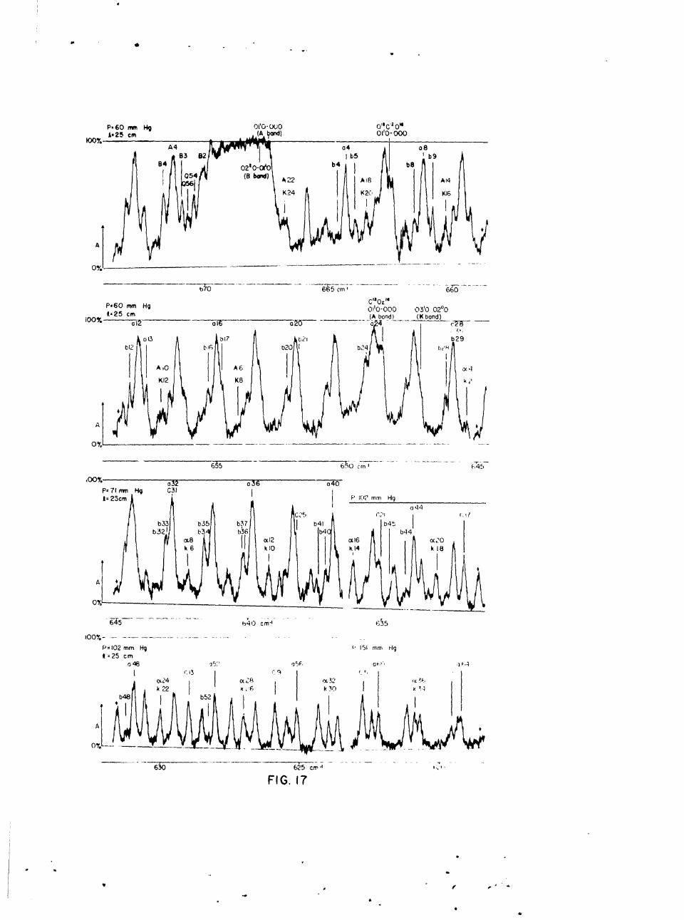
P,60 im IH 01'-OU lO O"C,20

A f" cm (A 2ond " )I 0 0 000

A4 I o4 08

84 02'0. 0 bo- 0 b b

05(5-)A2 A8 A 4

K24 K2(, K16

0%-

b7O 665 cm 660

P-60 mm Hg C3'00 030 0200

1 25 cm - (A bond) (K bond)all 016 a 0 - - 4C'8

i 13 b 17 I b29b12 bI, 20 b,4

AtO A6

K12 K(8

0% . ..

650 cm ',45

032 36 o40P-71 fm Hg C31

1t25cm ',i mm Hq

a,14

b33 b35 b37 b I b44b321 b3 b36 b4 b44

L82 o16 MOk6 ki 104 k48

o,!8At

0%

6-45 .. o cm-' 65

100%- --------- ..---- .. -

Ps102mm Hg -' 151 mm Hg1-25 cm

a48 '35: Q F- '

k k 30

60 625 cm-'

FIG. 17

Vi

(C~ 15WP-00 151m Hg£,25 con

, 0 68 o72 l

65 cm- 610

boy.

P4217 mm Hg0=25 cm P-306 mrn Hg

15 c19 c23 L4?

(F bond)

.... ~~20 111 ?0-C . .A F FI0 FS F7 F6 JF5 F4 F 21 f 3

0%.

605 600crr, b55

P, 306 mm Hgt 5 cm

c31 c35 c39 c43

1 4 5 f 6 7 f 8 1 0 f 1F 8

0%

590 cm- $,15

tO0% P rn' m jj

P,306 m Hg Int- 25 cm

A' f I4 1 f 22C - br h

0" a: - -- a , IIIW IIIv-

5FG cm8 546 r;44FIG. 18

v t.

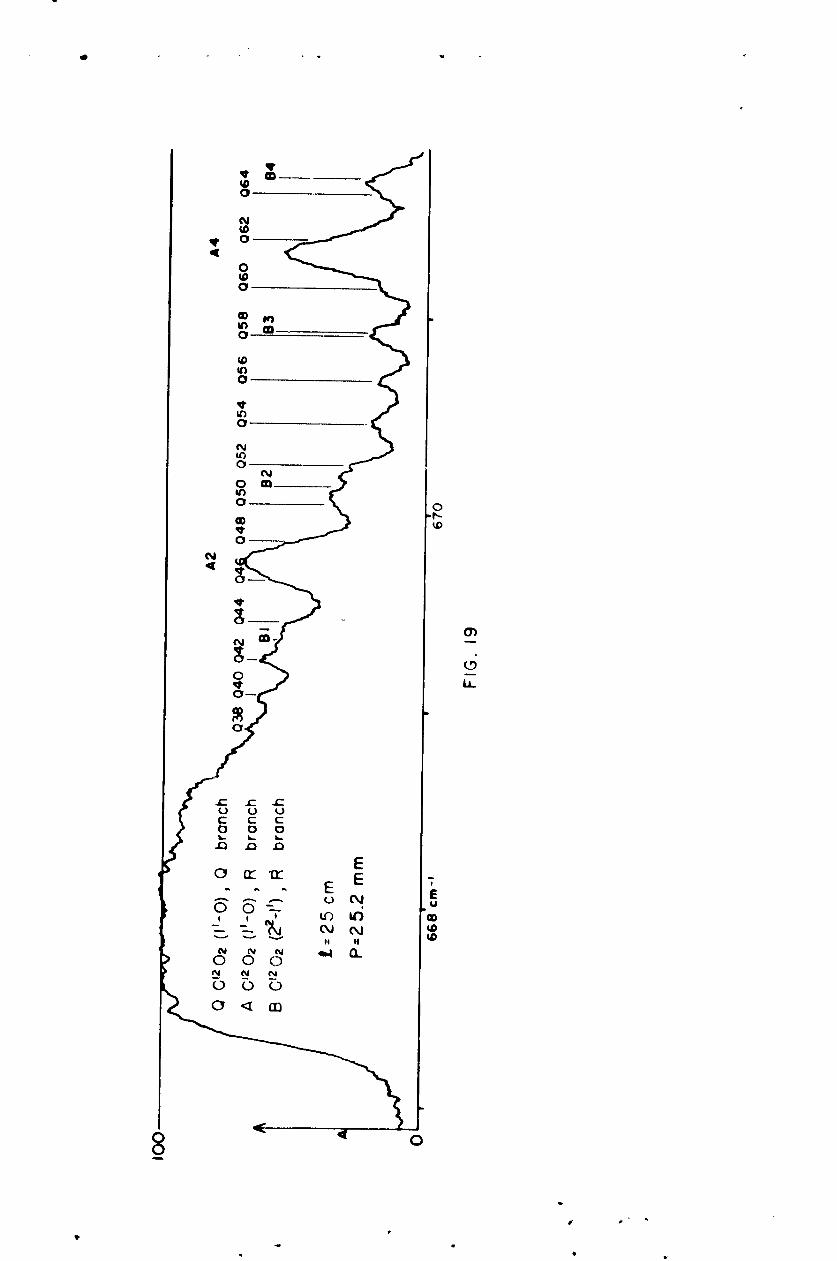
40

0 - -.

0

0

ina

40

In~0

V

00wIn

0-N4

N -Y

00

0-L

0 N .

.OD

8000

0 2.8

0.

00

S0 00

000

Lx 00

0 OD

N

cl.0

0' 0 N

_) _A____~~t u LO___

0Oal 0 GO

0 OD K)___

U)no

N N C, (0 0-

NN N j

N CON N~ in ro [

oo

10 0 U I

Iota. 'C.

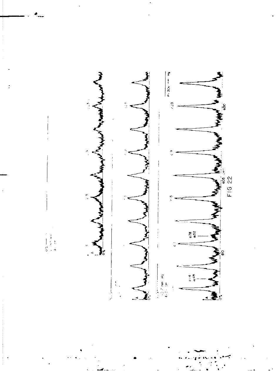
6

q 0~

0

to

OU-

'-II, L oy

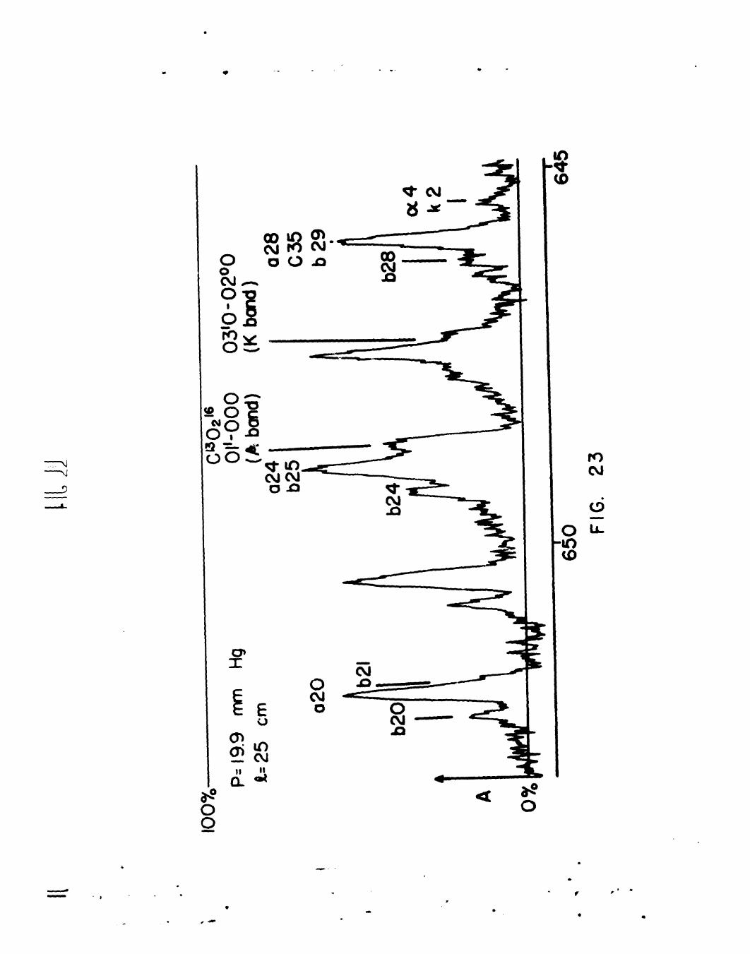
0

Oli

00

T 0LC', 0

0I-

o 0t

0.

4- 0

60

-0

02

oru

0 LL. 0

00

zY

fn

in 1Y- em

*0 -

or x 0

04 04

4 -0

aa

4CNo.*

404

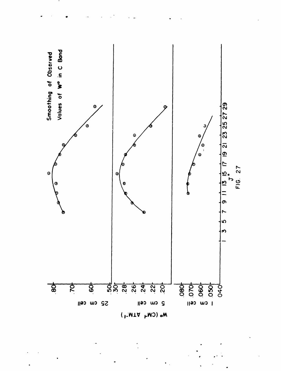
C) .V c

Sro

00k

OC

.- 0

0 C0

o o 6 0 *N N6E2

N N

0 N C*4

0 Ni

00 0 0 CD). (DV 00

0 0 ) 0

1103 3 110 wo Ia3 -

I-VYD) a

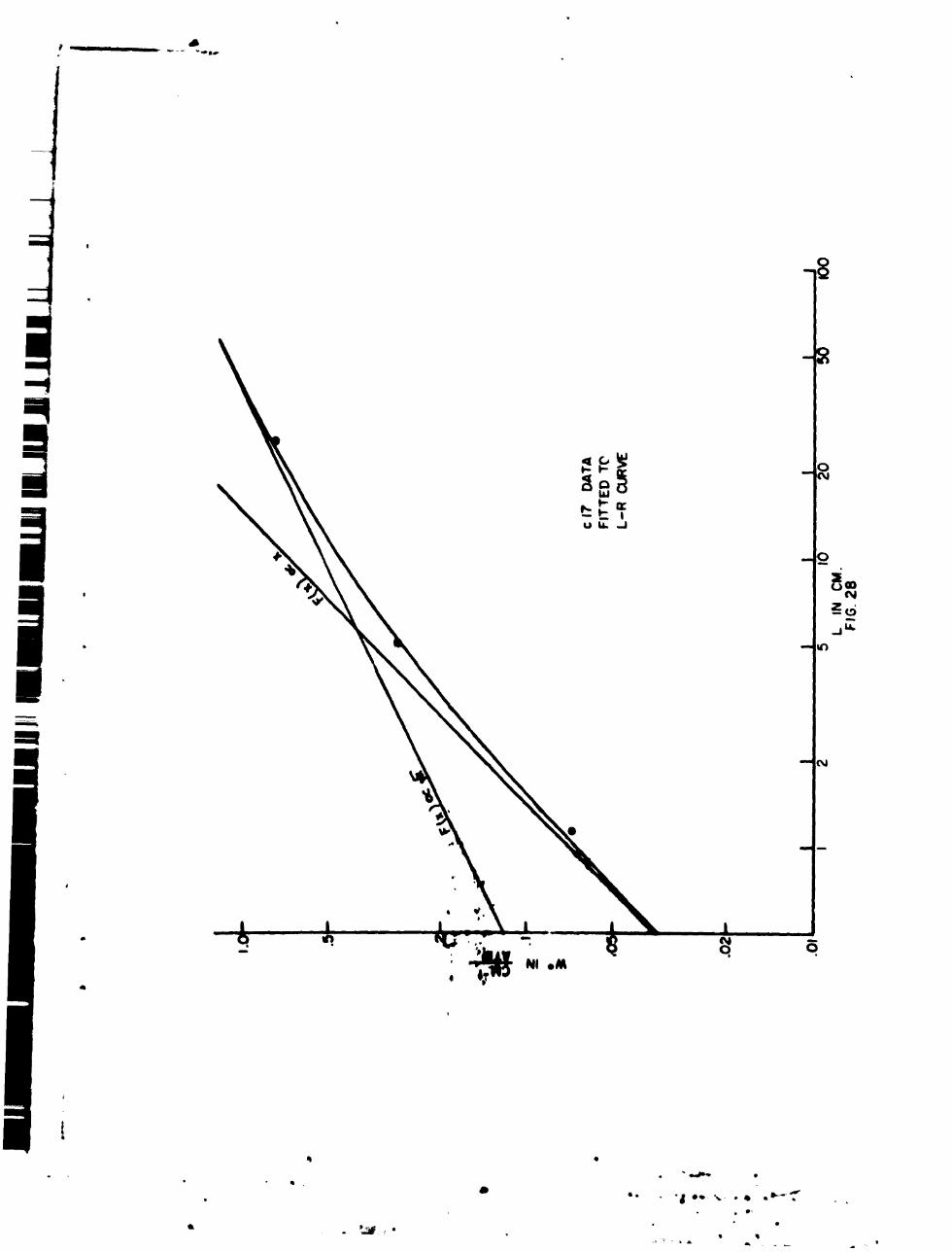
ii

THISPAGE

isMISSING

IN

ORIGINAL

DOC U IVJtIN 1

06 D termiflOti~ n of S o

f or Q Branch of F Band

E by Wilson SWells Method

0 FIG. 29

14 Determiflation Of So

f or 0 Branch of C Bond

1.2 by Wilson a Wells Method

.2 .4 .6 8 1.0 12 14 1.6

plL IN CM-ATM.FIG. 30

Iin

CS

0 1 N

(IK)00

xc 0

CD -- toqf* C00

7-W N0)

.9 C

E Nm

-Q In

c 1 . N

0 'c 0 I)VN

0 C0

0 0 0 0

N sN

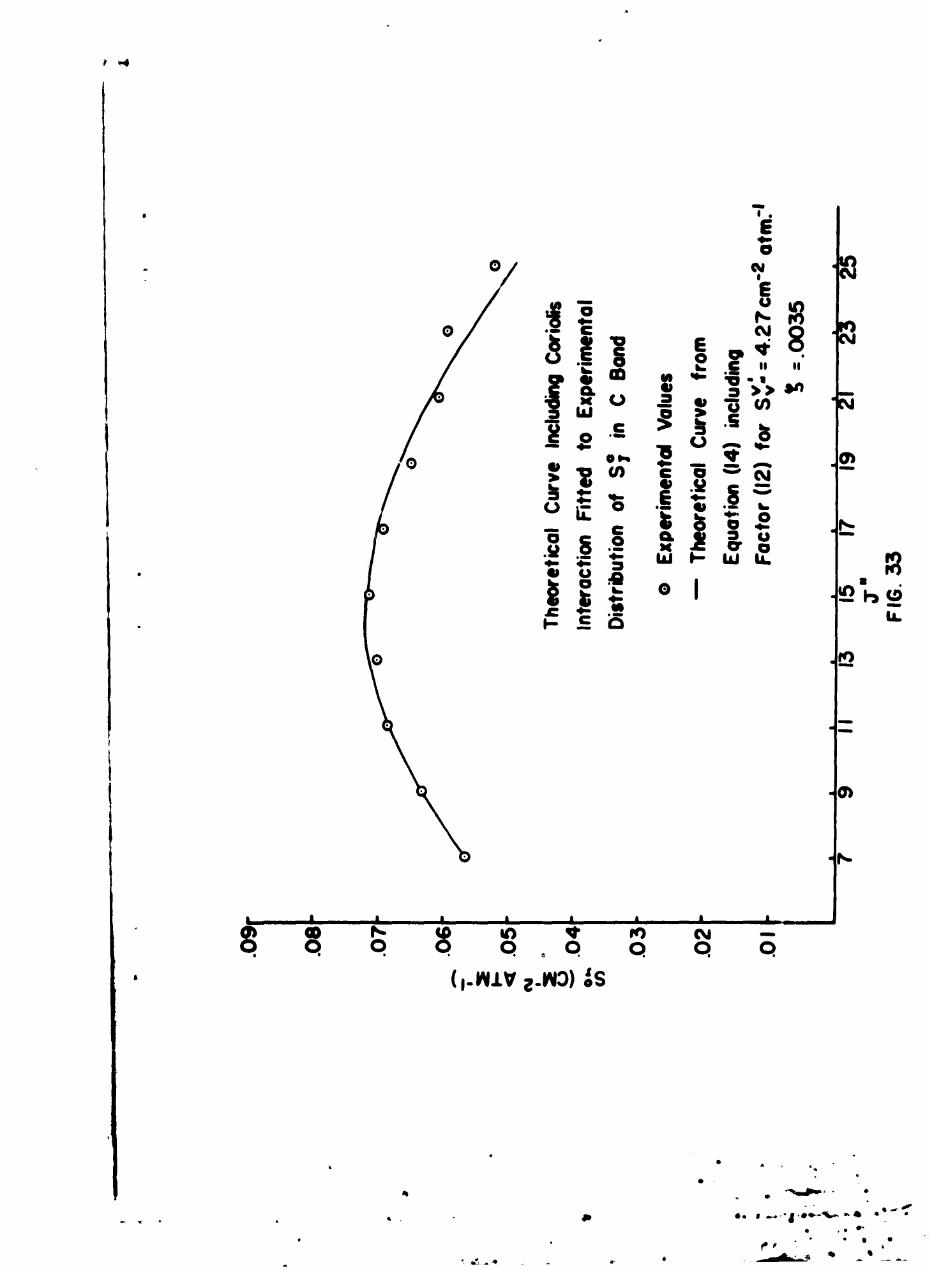
R5

0/ 8

c 11

c gg

ca C

4- 00 a c~

.C

fo

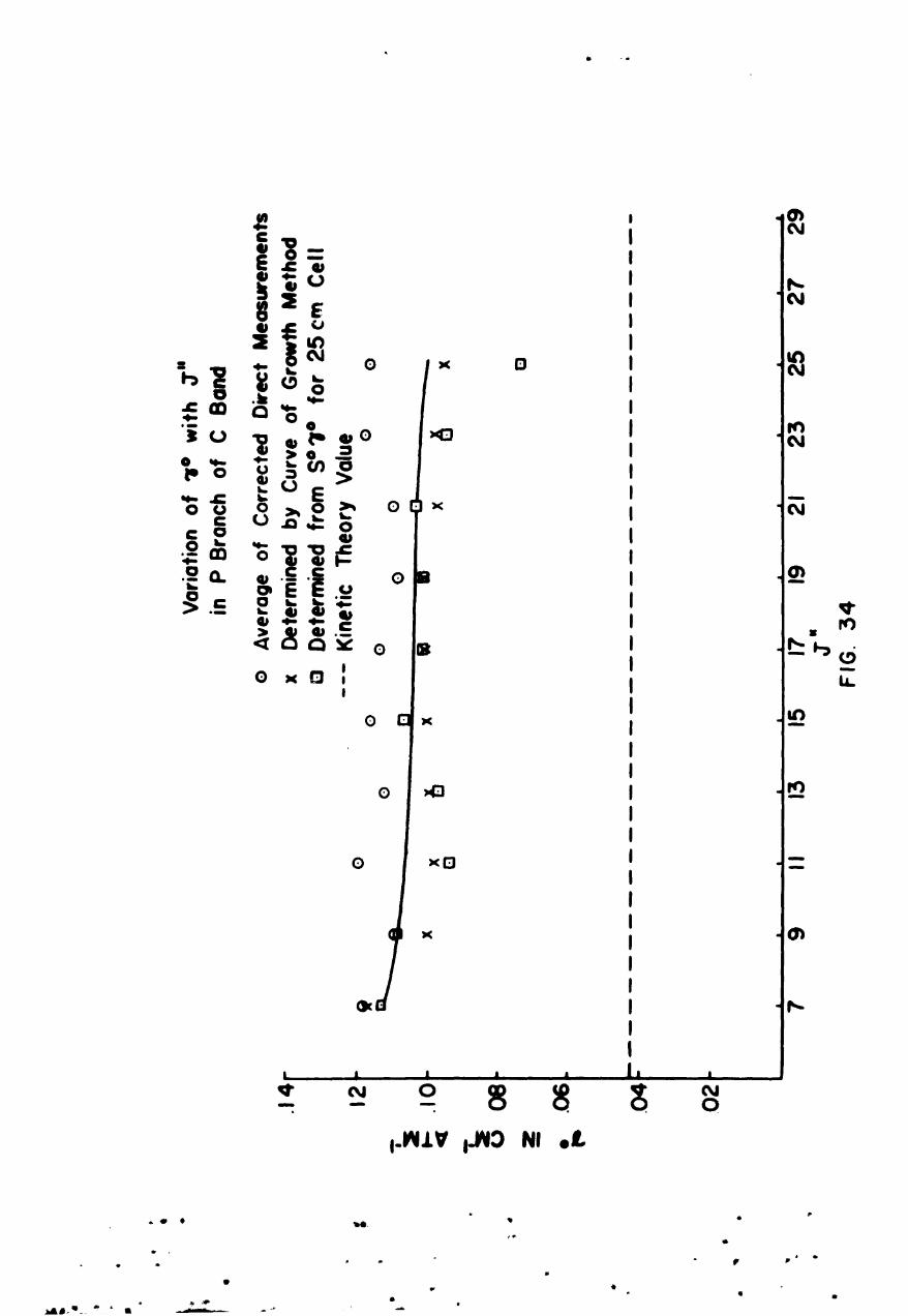
C NY

0 0

o No

0. C.I

2 E0- 0

oE M

0 3

0 B

00

0 I

0 7 0

II -Vi I -R NI II

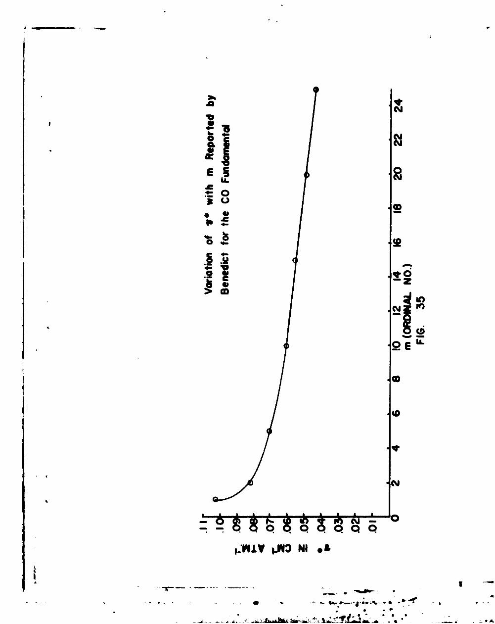
CMEn N

IL

E .c-C

C -zbe"0E -

10AW

NI

20

- - l *-

APIMDIX

Further Details of the Rotation and Drive Mechanisms

Pigure A is a sectional drawing of the grating turn-

table and axis of rotation. Figure B explains the geometry

of the cosine drive. An examination of these drawings and

of Figures 9 and 10 should make clear the text discussion

on pages 21-22.

It will be noted in Figure B that a cosine drive

may be obtained even though the drive arm is not normal

to the grating. This is made possible by fixing the drive

flat at an appropriate angle on the nut.

* - • *

iI

Grating Rib

Adjustable Grating Soutri BendDriv Ar SuportFace Plate

Fafnir MM309WI -CRRib Preloaded in tandem

SpectrometerFrame

Fafnir MM304WI-CRPre loaded back to back

Fig. A DETAILS OF GRATING TURNTABLESECTIONAL VIEW

Ir

CL

.9-

00

4 4-

0)

<

0.~0

MUE -C3'a' (5

lk. (. <

* ID *<