arindam banerjee- statistically steady measurements of rayleigh-taylor mixing in a gas channel
TRANSCRIPT

8/3/2019 Arindam Banerjee- Statistically Steady Measurements of Rayleigh-Taylor Mixing in a Gas Channel
http://slidepdf.com/reader/full/arindam-banerjee-statistically-steady-measurements-of-rayleigh-taylor-mixing 1/198
STATISTICALLY STEADY MEASUREMENTS OF RAYLEIGH-TAYLOR
MIXING IN A GAS CHANNEL
A Dissertation
by
ARINDAM BANERJEE
Submitted to the Office of Graduate Studies of
Texas A&M University
in partial fulfillment of the requirements for the degree of
DOCTOR OF PHILOSOPHY
August 2006
Major Subject: Mechanical Engineering

8/3/2019 Arindam Banerjee- Statistically Steady Measurements of Rayleigh-Taylor Mixing in a Gas Channel
http://slidepdf.com/reader/full/arindam-banerjee-statistically-steady-measurements-of-rayleigh-taylor-mixing 2/198
STATISTICALLY STEADY MEASUREMENTS OF RAYLEIGH-TAYLOR
MIXING IN A GAS CHANNEL
A Dissertation
by
ARINDAM BANERJEE
Submitted to the Office of Graduate Studies of Texas A&M University
in partial fulfillment of the requirements for the degree of
DOCTOR OF PHILOSOPHY
Approved by:
Chair of Committee, Malcolm J. AndrewsCommittee Members, Ali Beskok
Gerald MorrisonOthon Rediniotis
Head of Department, Dennis O’Neal
August 2006
Major Subject: Mechanical Engineering

8/3/2019 Arindam Banerjee- Statistically Steady Measurements of Rayleigh-Taylor Mixing in a Gas Channel
http://slidepdf.com/reader/full/arindam-banerjee-statistically-steady-measurements-of-rayleigh-taylor-mixing 3/198
iii
ABSTRACT
Statistically Steady Measurements of Rayleigh-Taylor Mixing in a Gas Channel.
(August 2006)
Arindam Banerjee, B.E., Jadavpur University;
M.S., Florida Institute of Technology
Chair of Advisory Committee: Dr. Malcolm J. Andrews
A novel gas channel experiment was constructed to study the development of
high Atwood number Rayleigh-Taylor mixing. Two gas streams, one containing air
and the other containing helium–air mixture, flow parallel to each other separated by
a thin splitter plate. The streams meet at the end of a splitter plate leading to the
formation of an unstable interface and of buoyancy driven mixing. This buoyancy
driven mixing experiment allows for long data collection times, short transients and
was statistically steady. The facility was designed to be capable of large Atwood
number studies of ABtB ~ 0.75. We describe work to measure the self similar evolution
of mixing at density differences corresponding to 0.035 < ABtB < 0.25. Diagnostics
include a constant temperature hot-wire anemometer, and high resolution digital
image analysis. The hot-wire probe gives velocity, density and velocity-density
statistics of the mixing layer. Two different multi-position single-wire techniques
were used to measure the velocity fluctuations in three mutually perpendicular
directions. Analysis of the measured data was used to explain the mixing as it
develops to a self-similar regime in this flow. These measurements are to our

8/3/2019 Arindam Banerjee- Statistically Steady Measurements of Rayleigh-Taylor Mixing in a Gas Channel
http://slidepdf.com/reader/full/arindam-banerjee-statistically-steady-measurements-of-rayleigh-taylor-mixing 4/198
iv
knowledge, the first use of hot-wire anemometry in the Rayleigh-Taylor community.
Since the measurement involved extensive calibration of the probes in a binary gas
mixture of air and helium, a new convective heat transfer correlation was formulated
to account for variable-density low Reynolds number flows past a heated cylinder. In
addition to the hot-wire measurements, a digital image analysis procedure was used
to characterize various properties of the flow and also to validate the hot-wire
measurements. A test of statistical convergence was performed and the study
revealed that the statistical convergence was a direct consequence of the number of
different large three-dimensional structures that were averaged over the duration of
the run.

8/3/2019 Arindam Banerjee- Statistically Steady Measurements of Rayleigh-Taylor Mixing in a Gas Channel
http://slidepdf.com/reader/full/arindam-banerjee-statistically-steady-measurements-of-rayleigh-taylor-mixing 5/198
v
ACKNOWLEDGEMENTS
I would like to thank my research advisor, Prof. Malcolm J. Andrews, for his
guidance, support and advice during the course of this work. This work has been funded
by the US Department of Energy under contract number DE-FG03-02NA00060. I also
wish to thank Wayne Kraft for his help in running the experiments and our numerous
discussions about the various diagnostics used in this work. Special thanks are also due
to Nicholas Mueschke, Michael Peart and Gopinath Subramanian for their help in
construction of the facility.
I would also like to thank my parents for giving me the love, values and virtues in
life. Their encouragement over the years has been the motivation in getting a doctoral
degree. Special thanks, love and appreciation are also due to my wife, Atrayee, for her
love, encouragement, support and being a part of this roller coaster life of a graduate
student. I wish her all the best for her dissertation work. I am also thankful to my
parents-in-law for being supportive over the years. Lastly and most importantly, I would
like to thank Dr. Kunal Mitra at Florida Tech for giving me the opportunity to pursue
higher studies in the United States and motivating me to pursue a career in research and
teaching.

8/3/2019 Arindam Banerjee- Statistically Steady Measurements of Rayleigh-Taylor Mixing in a Gas Channel
http://slidepdf.com/reader/full/arindam-banerjee-statistically-steady-measurements-of-rayleigh-taylor-mixing 6/198
vi
TABLE OF CONTENTS
Page
TABSTRACT……………………………………………………………………………..iii
UACKNOWLEDGEMENTSU ...............................................................................................v
TABLE OF CONTENTS ..................................................................................................vi
LIST OF FIGURES...........................................................................................................ix
LIST OF TABLES ......................................................................................................... xiii
U1. INTRODUCTIONU..........................................................................................................1
U1.1 BackgroundU ............................................................................................................1U1.2 Previous Rayleigh-Taylor ExperimentsU .................................................................5U1.3 Rayleigh-Taylor Experiments at Texas A&M U .....................................................10U1.4 Hot-Wire Anemometry - Advantages and LimitationsU........................................17U1.5 Objectives of Present ResearchU............................................................................20
U2. EXPERIMENTAL DESIGNU........................................................................................21
U
2.1 Experimental ApparatusU
.......................................................................................21U2.2 Mass Flow Rate CalibrationU.................................................................................26
U3. VISUALIZATION DIAGNOSTICSU ...........................................................................32
U3.1 Visualization Technique – CalibrationU................................................................32U3.2 Correction for Non-Uniform BacklightU...............................................................35U3.3 Steps in Image Processing DiagnosticsU...............................................................39U3.4 Qualitative MeasurementsU...................................................................................41
U4. HOT-WIRE DIAGNOSTICSU ......................................................................................45
U4.1 Constant Temperature Anemometry (CTA) for Measuring VelocityFluctuationsU ..............................................................................................45
U4.1.1 Calibration of a Single-Normal Hot-Wire Probe U .....................................48
U4.1.2 Hot-Wire Calibration EquationsU..............................................................51
U4.2 Constant Current Anemometry (CCA) for Measuring TemperatureFluctuationsU .............................................................................................57

8/3/2019 Arindam Banerjee- Statistically Steady Measurements of Rayleigh-Taylor Mixing in a Gas Channel
http://slidepdf.com/reader/full/arindam-banerjee-statistically-steady-measurements-of-rayleigh-taylor-mixing 7/198
vii
Page
U4.2.1 The Need for a CCA UnitU ........................................................................57
U4.2.2 The Cold (Resistance) Wire Probe U...........................................................59
U4.3 Single Wire MeasurementsU ..................................................................................61U4.3.1 Multi-Position Single Wire TechniqueU ..................................................61
U4.3.2 Multi-Position Multi-Overheat Single Wire TechniqueU.........................66
U5. CONVECTION CORRELATIONS FOR A HEATED WIRE U....................................84
U5.1 Heat Transfer Correlations from Heated Wires at Low Reynolds Number U.........84U5.2 Behavior of Hot-Wire/Film in Gas MixturesU .......................................................90U5.3 Effect of Temperature Jump on the Heat Transfer CoefficientU............................91U5.4 Convective Correlations for Binary Air-Helium MixtureU....................................94
U5.4.1 Properties of Gas MixturesU.......................................................................97
U
5.4.2 Effect of Binary Air-Helium MixtureU
......................................................99
U6. EXPERIMENTAL RESULTSU...................................................................................104
U6.1 PreliminariesU.......................................................................................................104U6.2 Measurements with Visualization AnalysisU .......................................................106
U6.2.1 Mixture Fraction MeasurementU..............................................................106
U6.2.2 Mix Width Measurement U .......................................................................109
U6.2.3 Test of ConvergenceU...............................................................................113
U6.2.4 Growth Constant (α) MeasurementU........................................................116
U6.3 Hot-Wire MeasurementsU ....................................................................................120U
6.3.1 Measurements with Multi-Position SN-Wire TechniqueU
.......................120 U6.3.2 Measurements with Multi-Position Multi-Overheat TechniqueU ............124
U6.4 Energy BudgetU....................................................................................................138
U7.CONCLUSIONSU.........................................................................................................140
ULITERATURE CITEDU ..................................................................................................144
UAPPENDIX A DESIGN BASISU ...................................................................................153
UA.1. Design Basis of the Experiment U .......................................................................153U
A.2 Gravity Current Effects in the Gas ChannelU
.....................................................156
UAPPENDIX B ERROR ANALYSISU ............................................................................160
UB.1. Error in Mass Flow Rate Measurement U............................................................160 UB.2. Error in Velocity MeasurementU ........................................................................160UB.3. Error in Atwood Number U..................................................................................161

8/3/2019 Arindam Banerjee- Statistically Steady Measurements of Rayleigh-Taylor Mixing in a Gas Channel
http://slidepdf.com/reader/full/arindam-banerjee-statistically-steady-measurements-of-rayleigh-taylor-mixing 8/198
viii
Page
UB.4 Error in VisualizationU .......................................................................................164UB.5 Error in Hot-Wire MeasurementU.......................................................................165
UAPPENDIX C PROPERTIES OF FLUIDSU..................................................................166
UC.1 Properties of HeliumU..........................................................................................166UC.2 Properties of Air U ................................................................................................166
UAPPENDIX D CALIBRATION CURVE FITS & ANALYSIS SOFTWAREU............167
UD.1 Table-Curve 3D Fits for E= F(U, ρ)U..................................................................167
UD.2 Table-Curve 3D Fits for E= F(U, θ)U..................................................................173 D.3 Matlab routine to solve for density-velocity correlations ...............................179
APPENDIX E. TWO FLUID INTERFACE IN ABSENCE OF SHEAR & BUOYANCY ....................................................................................181
VITA ..............................................................................................................................184

8/3/2019 Arindam Banerjee- Statistically Steady Measurements of Rayleigh-Taylor Mixing in a Gas Channel
http://slidepdf.com/reader/full/arindam-banerjee-statistically-steady-measurements-of-rayleigh-taylor-mixing 9/198
ix
LIST OF FIGURES
FIGURE Page
U1.1 Various stages of evolution of Rayleigh-Taylor instabilityU .....................................2
U1.2 Schematic of water channel facility at Texas A&M UniversityU ............................11
U1.3 Photograph of the water channel experiment,with nigrosene dye added to
the cold water streamU............................................................................................12
U1.4 Photograph of gas channel facility at Texas A&M UniversityU ..............................15
U1.5 Gas channel images of evolution of the R-T instability for AUBUtUBU # 0.04 U...................16
U2.1 Schematic of high Atwood number helium-air gas channel facility used for the experimentsU .....................................................................................................22
U2.2 Schematic of flow metering unit for a constant mass flow rate of heliumU..............27
U2.3 Calibration of mass flow rate of helium for different Atwood numbersU.................28
U3.1 Intensity as a function of height for calibration wedgeU...........................................34
U3.2 Histogram for raw imageU.........................................................................................37
U3.3 Histogram for processed imageU...............................................................................38
U3.4 View of the mixing process in the channel at (a) AUBUtUBU # 0.04 (U UBUmUBU = 50 cm/s)and (b) AUBUtUBU # 0.097 (U UBUmUBU = 85 cm/s)U...........................................................................42
U3.5 Close-up view of the three dimensional plumes across the channel for (a) AUBUtUBU # 0.04 (U UBUmUBU = 50 cm/s) and (b) AUBUtUBU # 0.097 (U UBUmUBU = 85 cm/s)U.............................43
3.6 Movie of the mixing process for AB
tB
# 0.259 (U B
mB
= 1.2 m/s)…………………….....44
U4.1 The constant temperature anemometer (CTA) circuitU.............................................46
U4.2 Schematic of setup used for hot-wire calibrationU....................................................50

8/3/2019 Arindam Banerjee- Statistically Steady Measurements of Rayleigh-Taylor Mixing in a Gas Channel
http://slidepdf.com/reader/full/arindam-banerjee-statistically-steady-measurements-of-rayleigh-taylor-mixing 10/198
x
FIGURE Page
U4.3 Variation in εUBUuUBU (goodness of fit) with exponent in power law relationshipfrom SN-wire calibration data in air at overheat ratio 0.6 over a velocity
range of 0.2-3 m/sU ..................................................................................................53
U4.4 Hot-wire calibration data (King’s law fit) in air at overheat ratio 1.9(∆T =257.14˚C) and 1.6 (∆T =171.43˚C)U..................................................................55
U4.5 Variation in King’s law constants for different volume fractions of heliumin a binary air-helium mixtureU.................................................................................56
U4.6 Calibration curve for cold wire (resistance wire) probeU............................................60
U4.7 Co-ordinate system for measurements and various orientations of hot-wire
used for measurementsU
............................................................................................64
U4.8 Wire orientations for multi-overheat multi-position techniqueU.................................71
U4.9 Velocity- density calibration for wire 1 at overheat ratio 1.9U ...................................74
U4.10 dE/dU for wire 1 at overheat ratio 1.9U.....................................................................75
U4.11 dE/d ρ for wire 1 at overheat ratio 1.9 U ....................................................................76
U4.12 Errors in voltage (%) for wire 1 at overheat ratio 1.9U .............................................77
U4.13 Directional calibration for wire 1 at overheat ratio 1.9U...........................................78
U4.14 Velocity- density calibration for wire 1 at overheat ratio 1.6U .................................79
U4.15 dE/dU for wire 1 at overheat ratio 1.6U.....................................................................80
U4.16 dE/d ρ for wire 1 at overheat ratio 1.6 U .....................................................................81
U4.17 Errors in voltage (%) for wire 1 at overheat ratio 1.6U .............................................82
U4.18 Directional calibration for wire 1 at overheat ratio 1.6U...........................................83
U5.1 Hot-wire calibrations in different volume fractions of helium in a binaryair-helium mixtureU...................................................................................................96
U5.2 Absolute viscosity and thermal conductivity of air-helium mixtureU........................98

8/3/2019 Arindam Banerjee- Statistically Steady Measurements of Rayleigh-Taylor Mixing in a Gas Channel
http://slidepdf.com/reader/full/arindam-banerjee-statistically-steady-measurements-of-rayleigh-taylor-mixing 11/198
xi
FIGURE Page
U5.3 Calibration at different overheat ratiosU...................................................................100
U5.4 Heat transfer correlation in a binary gas mixture of air and heliumU.......................103
U6.1 Close-up view of the three dimensional plumes across the channel for (a) AUBUtUBU # 0.04 (U UBUmUBU = 50 cm/s) and (b) AUBUtUBU # 0.097 (U UBUmUBU = 85 cm/s)U...........................107
U6.2 Contour levels (5%, 20%, 50%, 80% and 95%) plotted on average image
( N = 400) for an experimental run at ΑUBUtUBU # 0.035 (U UBUmUBU= 0.6 m/s)U ...........................108
U6.3 Mixture fraction distributions across the mixing layer for AUBUtUBU # 0.035U......................110
U6.4 Mixture fraction distributions across the mixing layer for AUBUtUBU # 0.259U.....................111
U6.5 Effect of number of images in average on the mixing widthU..................................112
U6.6 Percentage (%) root mean square error of density as a function of number of images (16 × 16 interrogation window) U............................................................115
U6.7 Comparison of growth constant (α UBU bUBU) measured with image diagnostics(gas channel) and PIV (water channel) U ................................................................117
U6.8 Comparison of growth constant (α UBU bUBU) obtained by image analysis (at gas channel)with LEM (Linear Electric Motor) experimental measurement of
Dimonte & Schneider (1996)U
................................................................................119
U6.9 α at the centerline plotted as a function of τ U...........................................................123
U6.10 Density profiles measured with the multi-position multi-overheat hot-wiretechnique.U ..............................................................................................................126
U6.11 Molecular mix parameters across the mix at τ = 1.986 (ΑUBUtUBU # 0.04, x = 1.75 m from the splitter plate). U........................................................................127
U6.12 Time evolution of scalar turbulence intensity and mix parameters measured
at the centerline (ΑUBUt UBU# 0.04).U ..................................................................................129
U6.13 Comparison of measured α by different techniques (Hot-wire: MPMO:Multi-Position Multi-Overheat Method; MP: Multi-Position Method)
at ΑUBUtUBU # 0.04. Water channel measurement was at ΑUBUtUBU # 7.5 x 10UPU
-4UPU.U.........................131
8/3/2019 Arindam Banerjee- Statistically Steady Measurements of Rayleigh-Taylor Mixing in a Gas Channel
http://slidepdf.com/reader/full/arindam-banerjee-statistically-steady-measurements-of-rayleigh-taylor-mixing 12/198
xii
FIGURE Page
U6.14 Velocity correlations across the mix at x = 1.75 m (τ =1.986) for anexperimental run at AUBUtUBU # 0.04U.................................................................................133
U6.15 Ratio of v'/u' across the mix at x = 1.75 m (τ =1.986) for an experimental
run at ΑUBUt UBU# 0.04U ......................................................................................................134
U6.16 Evolution of primary transport term for AUBUtUBU # 0.04U.................................................136
U6.17 Profile of < ρ 'v'> and < ρ 'u'> across the mix at τ = 1.986 for AUBUtUBU # 0.04U ..................137
UA.1 Stable configurations ( ρUBU1UBU > ρUBU2UBU) in a square box (1m × 1m) used to calculateconversion from potential energy to kinetic energy U..............................................158
E.1 Two fluid interface in absence of shear and density gradient (U BmB = 0.6 m/s)........182
E.2 Two fluid interface in absence of shear and density gradient (U BmB = 0.84 m/s)…..182
E.3 Two fluid interface in absence of shear and density gradient (U BmB = 1.2 m/s)…....183
E.4 Two fluid interface in absence of shear and density gradient (U BmB = 1.65 m/s)…..183

8/3/2019 Arindam Banerjee- Statistically Steady Measurements of Rayleigh-Taylor Mixing in a Gas Channel
http://slidepdf.com/reader/full/arindam-banerjee-statistically-steady-measurements-of-rayleigh-taylor-mixing 13/198
xiii
LIST OF TABLES
TABLE Page
U1.1 List of R-T experiments since 1950 and their respective authors, fluids used,Atwood number range obtained, mode of initial perturbation, diagnostics andexperimental run time.U...............................................................................................7
1.2 Comparison of design parameters between gas channel and water channel…..…...13
U1.3 Comparisons between Hot-Wire Anemometry (HWA), Particle ImageVelocimetry (PIV) and Laser Doppler Velocimetry (LDV) on the basis of therequirements in the gas channel facility U..................................................................18
U2.1 List of flow-straighteners and meshes in the inlet section of the facilityU................25
U2.2 Calibrated mass flow rates for different orificeU .......................................................29
U3.1 Camera (Canon Powershot A80) settings at different Atwood numbersU.................33
U4.1 Sample operating parameters for SN wire coupled to a mini-CTA unit(overheat ratio = 1.6)U..............................................................................................47
U4.2 Curve fits in the velocity range 0-3 m/s (calculated at overheat ratio 1.6)U ...............54
U4.3 Various measurement orientations for multi-position measurement techniqueU........65
U4.4 Wire properties at overheat ratios 1.9 and 1.6U...........................................................70
U4.5 Various measurement orientations for multi-position measurement techniqueU........72
U5.1 Convection heat transfer correlations for flow over a heated cylinder U .....................88
U5.2 List of convection heat transfer correlations involving hot-wire anemometry(small cylinders)U......................................................................................................89
U5.3 Sample calculations for various correlation parameters for air U...............................102
U6.1 List of imaging and hot-wire experimentsU .............................................................105

8/3/2019 Arindam Banerjee- Statistically Steady Measurements of Rayleigh-Taylor Mixing in a Gas Channel
http://slidepdf.com/reader/full/arindam-banerjee-statistically-steady-measurements-of-rayleigh-taylor-mixing 14/198
xiv
TABLE Page
U6.2 Velocity fluctuations (m/s) measured at AUBUtUBU # 0.035 (U UBUmUBU= 0.6 m/s)U........................122
UA.1 Minimum flow velocity to satisfy parabolic approximation in gas channelU ..........155
UA.2 Vertical velocity (v) of the gravity wave and mean flow velocity U UBUm UB Ucorresponding to different run conditions at a different Atwood numbers( L = 0.6m).U.............................................................................................................159
UB.1 Uncertainty in Atwood Number for various experimental run conditionsU.............163

8/3/2019 Arindam Banerjee- Statistically Steady Measurements of Rayleigh-Taylor Mixing in a Gas Channel
http://slidepdf.com/reader/full/arindam-banerjee-statistically-steady-measurements-of-rayleigh-taylor-mixing 15/198
1
1. INTRODUCTION
1.1 Background
Rayleigh-Taylor (R-T) instability may be induced when a heavy fluid is placed over
a light fluid in a gravitational field. If the planar surface between the two fluids is
disturbed with a perturbation of finite amplitude, the disturbances are driven by
buoyancy and develop as R-T instability (Rayleigh 1884; Taylor 1950). The interface
becomes distorted with time and the wavelengths associated with the initial disturbance
interact between themselves causing a mingling process to degenerate into a turbulent
mix. Development of the TP
PT mix was divided by Youngs (1984) into three successive
regimes. The mix starts with an initial exponential growth of infinitesimal perturbations
that correspond with linear stability analysis. At amplitude about one-half of the
wavelength, the linear growth regime of the instability saturates and the perturbation
speed settles to at a constant rate. Thereafter, longer wavelengths overtake due to their
continuing exponential growth, a phenomenon referred to as “bubble competition”
(Emmons et al. 1960). Eventually, a self-similar R-T mix layer is formed through mode
interaction and successive wavelength saturation. The three stages have been illustrated
in Figure 1.1.
Once at self similarity, and with loss of memory of the initial conditions, dimensional
analysis suggests that the mixing half-width grows quadratically with time according to
the relation, 2 gt h ∝ , where, t , is the time and g , the acceleration due to gravity.
TP
PT This dissertation follows the style and format of the Annual Review of Fluid Mechanics.

8/3/2019 Arindam Banerjee- Statistically Steady Measurements of Rayleigh-Taylor Mixing in a Gas Channel
http://slidepdf.com/reader/full/arindam-banerjee-statistically-steady-measurements-of-rayleigh-taylor-mixing 16/198
2
Figure 1.1 Various stages of evolution of Rayleigh-Taylor instability.
Stage 1 - Exponential growth of infinitesimal perturbations; Stage 2 – Saturation of the initial perturbations; and Stage 3 – Bubble competition. Images are taken from 3D-
DNS with a resolution of 256 × 128 × 256 by Mueschke (2004).
Heavy
Light

8/3/2019 Arindam Banerjee- Statistically Steady Measurements of Rayleigh-Taylor Mixing in a Gas Channel
http://slidepdf.com/reader/full/arindam-banerjee-statistically-steady-measurements-of-rayleigh-taylor-mixing 17/198
3
However, experiments and computations (Anuchina et al. 1978 ; Youngs 1984) suggest
that a more complete description was given by:
2,, gt Ah t sb sb α = (b:bubble; s:spike) (1.1)
where the Atwood number, ABtB, denotes the governing parameter of the flow defined
by )()( 2121 ρ ρ ρ ρ +−≡t A ; ρ B1B and ρ B2B are the densities of air (heavy fluid) and air-
helium mixture (light fluid) employed in the present work; hBb Band hBsB were the heights
(above/below the density interface) of the “rising” bubbles and the “falling” spikes
respectively; α B
bB
and αB
sB
denotes the growth rate constants (for the bubbles and spikes)
which was to be determined. For low Atwood numbers (< 0.1), the mix is symmetric ( hB b
B= hBsB) and α was usually taken as a constant, i.e. α B b B= α BsB = α (Dimonte 1999; Ramaprabhu
& Andrews 2004). However, for high Atwood numbers (≥ 0.1), the mix is no longer
symmetric about the density interface (hBs B> hB bB). The values of α is found to be different
(α B b B< α BsB) with α BsB being a function of the Atwood number and α B bB was approximately
constant (Dimonte 1999; Dimonte & Schneider 1996). Equation (1.1) for h was obtained
by Youngs (1984) by using a nonlinear extension of the linear stability theory
(Chandrasekhar 1961).
R-T flows represent a canonical fluid flow that encompasses the laminar, transition
and turbulent flow regimes. A complete understanding of R-T flows is desired because of
the broad impact such flows have in nature and a variety of applications, in particular, in
buoyancy and shock driven instabilities which occur during the implosion phase of
Inertial Confinement Fusion (ICF) process (Lindl 1998; Roberts et al. 1980). An ICF
process involves high power laser or x-ray bombardment of target fuel capsules

8/3/2019 Arindam Banerjee- Statistically Steady Measurements of Rayleigh-Taylor Mixing in a Gas Channel
http://slidepdf.com/reader/full/arindam-banerjee-statistically-steady-measurements-of-rayleigh-taylor-mixing 18/198
4
(deuterium-tritium pellets). Implosion of the pellets to a super-dense state necessary for
thermonuclear burn requires a spherical symmetry (Clarke et al. 1973). Surface
imperfections in the pellets and drive asymmetries lead to unavoidable departures from
this spherical symmetry which gives rise to the hydrodynamic instabilities. The
acceleration phase of an ICF capsule is Richtmeyer-Meshkov (R-M) unstable, while the
late-time deceleration phase is Rayleigh-Taylor unstable (Lindl 1998; Roberts et al.
1980). The R-M Instability is an impulsively driven variant of the R-T Instability
(Brouillette 2002; Meshkov 1969; Richtmyer 1960). The growth of the R-T driven
mixing layer has been shown to be the limiting factor for the yield of the ICF process
(Atzeni & Meyer-ter-Vehn 2004; Betti et al. 2001; Lindl 1998).
In astrophysics, the formation of fast optical filaments in a young supernova has
been attributed to Rayleigh-Taylor instability as the expanding sphere sweeps up
interstellar material (Gull 1975). It was assumed that the limiting factor in the creation of
the heavy interstellar elements in collapsing stars was the growth of the mixing layer
formed by adverse density stratification in its gravitational field (Smarr et al. 1981). R-T
generated turbulence also occurs in geophysical formations like salt domes and volcanic
islands (DiPrima & Swinney 1981); in deep-sea ocean currents and in rivers and
estuaries (Cui & Street 2004; Molchanov 2003). The breakup of fuel droplets in high
speed flows have also been found to be R-T unstable (Marmottant & Villermaux 2004;
Thomas 2003). Experiments performed to study atomization of a liquid jet when a fast
gas stream blows parallel to its surface show that the liquid destabilization proceeds
from a two-stage mechanism: a shear instability first forms waves on the liquid. The
8/3/2019 Arindam Banerjee- Statistically Steady Measurements of Rayleigh-Taylor Mixing in a Gas Channel
http://slidepdf.com/reader/full/arindam-banerjee-statistically-steady-measurements-of-rayleigh-taylor-mixing 19/198
5
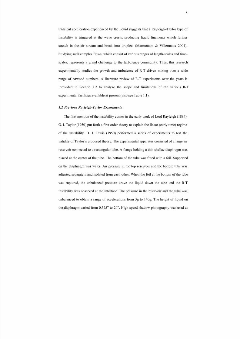
transient acceleration experienced by the liquid suggests that a Rayleigh–Taylor type of
instability is triggered at the wave crests, producing liquid ligaments which further
stretch in the air stream and break into droplets (Marmottant & Villermaux 2004).
Studying such complex flows, which consist of various ranges of length-scales and time-
scales, represents a grand challenge to the turbulence community. Thus, this research
experimentally studies the growth and turbulence of R-T driven mixing over a wide
range of Atwood numbers. A literature review of R-T experiments over the years is
provided in Section 1.2 to analyze the scope and limitations of the various R-T
experimental facilities available at present (also see Table 1.1).
1.2 Previous Rayleigh-Taylor Experiments
The first mention of the instability comes in the early work of Lord Rayleigh (1884).
G. I. Taylor (1950) put forth a first order theory to explain the linear (early time) regime
of the instability. D. J. Lewis (1950) performed a series of experiments to test the
validity of Taylor’s proposed theory. The experimental apparatus consisted of a large air
reservoir connected to a rectangular tube. A flange holding a thin shellac diaphragm was
placed at the center of the tube. The bottom of the tube was fitted with a foil. Supported
on the diaphragm was water. Air pressure in the top reservoir and the bottom tube was
adjusted separately and isolated from each other. When the foil at the bottom of the tube
was ruptured, the unbalanced pressure drove the liquid down the tube and the R-T
instability was observed at the interface. The pressure in the reservoir and the tube was
unbalanced to obtain a range of accelerations from 3g to 140g. The height of liquid on
the diaphragm varied from 0.375” to 20”. High speed shadow photography was used as

8/3/2019 Arindam Banerjee- Statistically Steady Measurements of Rayleigh-Taylor Mixing in a Gas Channel
http://slidepdf.com/reader/full/arindam-banerjee-statistically-steady-measurements-of-rayleigh-taylor-mixing 20/198
6
diagnostics and the run time obtained was ~ 10P
-2Pseconds. However, both Taylor and
Lewis did not take into consideration effects of surface tension and viscosity on the rate
of growth of the instability and studied the instability on fluid combinations like air-
benzene, air-water and air-glycerin. Allred and Blount (1954) included the effects of
surface tension and fluid viscosity in their experiments by choosing a combination of
water and n-heptane / isoamyl alcohol / n-octyl alcohol as the working fluids. They used
an apparatus similar to that of Lewis (1950). Using these fluid combinations lowered the
interfacial tension between the two fluids by a factor of 20 as the other fluid properties
remained unchanged. The Atwood number range obtained (Allred & Blount 1954; Lewis
1950) was between 0.1 and 0.99.
The R-T instability has also been studied by accelerating an initially stable stratified
mixture of two fluids by using a variety of mechanisms like rubber cords (Emmons et al.
1960), bungee/elastic cords (Ratafia 1973) and compressed air (Cole & Tankin 1973).
The objective of these experiments was to excite a particular eigenmode of the surface
and then to accelerate the stratified mixture when the initial perturbations had a
prescribed amplitude and phase. However, majority of the experiments described above
(Cole & Tankin 1973; Emmons et al. 1960; Ratafia 1973) used a vibrating paddle for
generating the initial perturbations which resulted in generation of a wide spectrum of
modes instead of a single eigenmode (Popil & Curzon 1979). The phase of such modes
and their amplitudes were variable and thus, the experiments were not repeatable. Popil
and Curzon (1979) used a electrostatic generator to accurately generate single-mod

8/3/2019 Arindam Banerjee- Statistically Steady Measurements of Rayleigh-Taylor Mixing in a Gas Channel
http://slidepdf.com/reader/full/arindam-banerjee-statistically-steady-measurements-of-rayleigh-taylor-mixing 21/198
TABLE 1.1 List of R-T experiments since 1950and their respective authors, fluids used, Atwood mode of initial perturbation, diagnostics and experimental run time
Year Authors Fluids Atwood # Mode 2D/3D Diag
1950 Lewis A/B, A/G & A/W 0.99 S 2D Im
1954 Allred et. al. W/nH, W/OA, W/I, nH/A 0.188-0.995 S 2D Im
1960 Emmons et. al. CT/A & M/A 0.107,0.997 S 2D Im
1973 Ratafia OA/W 0.095 S 2D Im
1973 Cole & Tankin A/W 0.99 S 2D Im
1979 Popil &Curzon A/W 0.99 S + M 2D Im
1984 Read W/P, SI/P, EA/A 0.231-0.997 M 2D/3D Im
1986, 1990 Andrews & Spalding Br/W 0.048 M 2D Im
1985 – 2005 Jacobs et al. A/W 0.99 M 3D Im
1991, 1994 Linden & Redondo Br/W 10P
-4P to 0.05 M 3D
ImagiCondmeasu
1993, 1999 Dalziel et al. Br/(W + P2) 2×10P
-3P to 7×10P
-4P M 3D L
1994- 2004 Andrews et al. Hot W-Cold W 10P
-4P to 10P
-3P M 3D
ImagiTherm
1996- 2004 Dimonte & Schneider S/H, S/BT,Various 0.15 - 0.96 M 2D LIF &
1997 - 2003 Kucherenko et al. G/B, W/Hg, W/Kl,
B/(W+G)/SHS0.23 - 0.5 M 3D
Pulse photo
2004 - present
Andrews and Banerjee A/H 0.035-0.75 M 3D Imaging
Index for Fluids:A: Air, Al: Alcohol, B: Benzene, Br: Brine, BT: Butane, CT: Carbon Tetrachloride, EA: Ethyl Alcohol, G: Glycerin, H
Amyl Alcohol, Kl: Klerichi liquid (Formic-Malonic Acid Talium), M: Methanol, nH: n-Heptane; OA: Octyl Alcohol, P
Petrol; S: SFB6B, SI: Sodium Iodide, SHS: Sodium Hyposulfite, W: Water

8/3/2019 Arindam Banerjee- Statistically Steady Measurements of Rayleigh-Taylor Mixing in a Gas Channel
http://slidepdf.com/reader/full/arindam-banerjee-statistically-steady-measurements-of-rayleigh-taylor-mixing 22/198
8
standing waves on the water interface. A timing circuit was wired along with the wave
generator to control the time of release and subsequent acceleration of the tank. By
controlling the number of electrodes in the electrostatic generator, single or multi-mode
excitations was induced at the interface and the experiment was thus more repeatable.
A major drawback of the experiments described above was that they were all
conducted in narrow long cavities and were two-dimensional. To examine three-
dimensional turbulent mixing layers, Read (1984) used rockets to accelerate an initially
stable stratified mixture downwards. He obtained accelerations of 25g - 75g by using
this method. Jacobs and Caton (1988) accelerated a small volume of water down a
vertical tube using compressed air. They used high speed motion picture photography to
study 3D Rayleigh-Taylor Instability in a round and square tube with acceleration
varying between 5g to 10g. Andrews and Spalding (1990) created an unstable buoyancy
gradient by quickly inverting a stable stratified mixture. Linden et al. (1992) and Dalziel
et al. (1999) placed a heavy fluid over a light fluid, separated by a thin plate. The plate
was withdrawn and buoyancy driven mixing ensued between the two fluids. Recently,
Jacobs and Dalziel (2005) studied R-T instability in a system of three fluids using the
same technique. The stratification consists of one stable and one unstable interface and
was formed by using different salt solutions and fresh water. Kucherenko (2003; 1997)
used a drop tank technique that was accelerated using a gas gun to achieve accelerations
between 100g to 350g. He used an aqueous solution of glycerin and benzene to give
Atwood numbers ranging from 0.23 to 0.5. Diagnostics used included pulsed x-ray
photography. Dimonte et al. (1999; 1996) studied turbulent RT growth rates over a

8/3/2019 Arindam Banerjee- Statistically Steady Measurements of Rayleigh-Taylor Mixing in a Gas Channel
http://slidepdf.com/reader/full/arindam-banerjee-statistically-steady-measurements-of-rayleigh-taylor-mixing 23/198
9
comprehensive range of Atwood numbers (0.1304 – 0.961) with constant acceleration
using the Linear Electric Motor. Diagnostics involved bi-level LIF (Laser Induced
Fluorescence) measurements and backlight photography. However, a major drawback of
these experiments was that they all used complicated mechanisms like rockets, fast-
sliding plates and linear electric motors to generate the R-T instability. In addition, all
these experiments were transient studies with short data capture times (~0.001 – 5
second). Thus, a large number of repeated experiments were needed to collect statistical
data sets.
Over the past two decades, advances in modeling of variable density turbulence has
led to introduction of various turbulence models which includes: spectral transport
models (Besnard et al. 1990; 1992; Steinkamp et al. 1995), two-fluid models (Andrews
1986; Youngs 1989) and Reynolds Stress/Bousinesq models (Snider & Andrews 1996).
Validation of predictive turbulent transport models consisting of inhomogeneous,
anisotropic and variable-density flows require a priori knowledge of various velocity,
density and velocity-density correlations like 222 ',','','',' vuvu ρ ρ ρ and ''vu . These
quantities may be computed from direct numerical simulation (DNS). Cook and
Dimotakis (2001) performed DNS of 256P
2P×1024 reaching a Taylor Reynolds number of
100; which was the proposed threshold for mixing transition (Dimotakis 2000). Cook et
al. (2004) used a very high resolution large-eddy-simulation (1152 P
3P) to further
investigate the asympototic growth of the mixing layer. Such a simulation constitutes
one realization of the mixing layer and was a typical state-of-the-art DNS of R-T mixing.

8/3/2019 Arindam Banerjee- Statistically Steady Measurements of Rayleigh-Taylor Mixing in a Gas Channel
http://slidepdf.com/reader/full/arindam-banerjee-statistically-steady-measurements-of-rayleigh-taylor-mixing 24/198
10
However, such calculations were limited to low-Reynolds numbers. Thus, there is a need
to experimentally determine these quantities.
1.3 Rayleigh-Taylor Experiments at Texas A&M
A water-channel facility, built at Texas A&M University in the early 1990’s
addressed these deficiencies (Snider & Andrews 1994). The facility uses a novel
experimental setup which eliminates complex mechanisms like rockets, fast sliding
plates, elastic cords, linear electric motors or compressed air cannons. Two streams of
fluid, cold water (heavy) on top and hot water (light) at the bottom (see Figure 1.2) flow
parallel to each other separated by a thin splitter plate . The streams meet at the end of a
splitter plate creating an unstable interface which leads to buoyancy mixing, albeit at
small ABt B ~ 10P
-4P - 10P
-3P(Ramaprabhu & Andrews 2004; Snider 1994; Snider & Andrews
1994; 1995; Wilson 2002; Wilson et al. 1999; Wilson & Andrews 2002). The water
channel setup is similar to a shear flow experiment. A combined buoyancy and shear
mixing layer can also be obtained if the velocities of the top and bottom streams are
different. If the velocities are identical, a buoyancy mixing layer is obtained. The facility
allows long run times of ~ 600 seconds, thus allowing measurement of higher order
statistics.
The basis of the water channel experiment is a Galilean transformation from a
moving frame of reference at the mean convective velocity to a transient frame of
reference (Snider 1994). For this, the experimental flow should be parabolic, i.e. a one-
way characteristic was essential where downstream conditions do not affect the upstream
behavior. It has been well established from boundary layer-type assumptions that shear

8/3/2019 Arindam Banerjee- Statistically Steady Measurements of Rayleigh-Taylor Mixing in a Gas Channel
http://slidepdf.com/reader/full/arindam-banerjee-statistically-steady-measurements-of-rayleigh-taylor-mixing 25/198
11
Figure 1.2 Schematic of water channel facility at Texas A&M University
(Ramaprabhu & Andrews 2004).
UE-type thermocouplesU
Nickel-Chromium andConstantanJunction diameter of 0.01-0.02 cmResponse time 0.001 s/P
oPC
Acquisition rate 100 Hz.
0.3 m
0.2 m
1.0mHot Water Cold Water
UCamera640H x 480V Pixels1200 Image Capacity onBoard
ULasersTwo 120 mJ15 Hz pulse
Sample rate: 30/sec.
UPIV/PLIF Imagefield
8 cm Hort.x 6 cm Vert.

8/3/2019 Arindam Banerjee- Statistically Steady Measurements of Rayleigh-Taylor Mixing in a Gas Channel
http://slidepdf.com/reader/full/arindam-banerjee-statistically-steady-measurements-of-rayleigh-taylor-mixing 26/198
12
Figure 1.3 Photograph of the water channel experiment, with nigrosene dye added to thecold water stream. The evolution of the mix was quadratic in x (downstream coordinate),with the mix width depending on the Atwood number ( ABt B), and g , the acceleration due togravity. In this experiment, the distance downstream can be related to time through the
Taylor’s hypothesis.
10 cm
Flow directionCold water
Warm water

8/3/2019 Arindam Banerjee- Statistically Steady Measurements of Rayleigh-Taylor Mixing in a Gas Channel
http://slidepdf.com/reader/full/arindam-banerjee-statistically-steady-measurements-of-rayleigh-taylor-mixing 27/198
13
TABLE 1.2 Comparison of design parameters between gas channel and water channel
Parameter Water Channel Gas Channel
Medium Hot/Cold Water Air-Helium
Atwood number 0.001 0.75
Dimensions ( L × B × H ) 1.0 m × 0.3 m × 0.2 m 2.0 m × 0.6 m × 0.4 m
ReBmaxB ( )
mix
mt h gA
ν
23
2
6= ~ 2400 ~ 20000
U BmB 0.05 m/s 2.0 m/s
DiagnosticsImaging, Thermocouple,
PIV, PLIF
Imaging, Hot-wireanemometry, Cold-wire
anemometry
Cost of run ~ $0 $33 per bottle
8/3/2019 Arindam Banerjee- Statistically Steady Measurements of Rayleigh-Taylor Mixing in a Gas Channel
http://slidepdf.com/reader/full/arindam-banerjee-statistically-steady-measurements-of-rayleigh-taylor-mixing 28/198
14
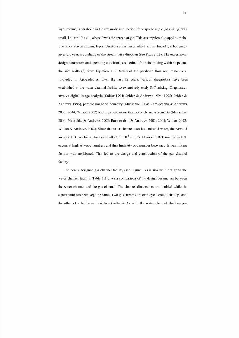
layer mixing is parabolic in the stream-wise direction if the spread angle (of mixing) was
small, i.e. 1tan 2 <<θ , where θ was the spread angle. This assumption also applies to the
buoyancy driven mixing layer. Unlike a shear layer which grows linearly, a buoyancy
layer grows as a quadratic of the stream-wise direction (see Figure 1.3). The experiment
design parameters and operating conditions are defined from the mixing width slope and
the mix width (h) from Equation 1.1. Details of the parabolic flow requirement are
provided in Appendix A. Over the last 12 years, various diagnostics have been
established at the water channel facility to extensively study R-T mixing. Diagnostics
involve digital image analysis (Snider 1994; Snider & Andrews 1994; 1995; Snider &
Andrews 1996), particle image velocimetry (Mueschke 2004; Ramaprabhu & Andrews
2003; 2004; Wilson 2002) and high resolution thermocouple measurements (Mueschke
2004; Mueschke & Andrews 2005; Ramaprabhu & Andrews 2003; 2004; Wilson 2002;
Wilson & Andrews 2002). Since the water channel uses hot and cold water, the Atwood
number that can be studied is small ( ABt B ~ 10P
-4P - 10P
-3P). However, R-T mixing in ICF
occurs at high Atwood numbers and thus high Atwood number buoyancy driven mixing
facility was envisioned. This led to the design and construction of the gas channel
facility.
The newly designed gas channel facility (see Figure 1.4) is similar in design to the
water channel facility. Table 1.2 gives a comparison of the design parameters between
the water channel and the gas channel. The channel dimensions are doubled while the
aspect ratio has been kept the same. Two gas streams are employed, one of air (top) and
the other of a helium–air mixture (bottom). As with the water channel, the two gas

8/3/2019 Arindam Banerjee- Statistically Steady Measurements of Rayleigh-Taylor Mixing in a Gas Channel
http://slidepdf.com/reader/full/arindam-banerjee-statistically-steady-measurements-of-rayleigh-taylor-mixing 29/198
15
Figure 1.4 Photograph of gas channel facility at Texas A&M University.
Honeycomb
Inletducting
UG ResearchAsst. (6ft tall)
Exit plenum
Flow channel
Splitter plate Meshes
Fans
Air
He

8/3/2019 Arindam Banerjee- Statistically Steady Measurements of Rayleigh-Taylor Mixing in a Gas Channel
http://slidepdf.com/reader/full/arindam-banerjee-statistically-steady-measurements-of-rayleigh-taylor-mixing 30/198
16
Figure 1.5 Gas channel images of evolution of the R-T instability for ABtB # 0.04
(U BmB = 0.5 m/s). A parabolic profile was fitted on mixing width (α B bB = 0.07). Green smokewas added to the bottom stream for visualization purpose.
Air
Air + He
+ Smoke

8/3/2019 Arindam Banerjee- Statistically Steady Measurements of Rayleigh-Taylor Mixing in a Gas Channel
http://slidepdf.com/reader/full/arindam-banerjee-statistically-steady-measurements-of-rayleigh-taylor-mixing 31/198
17
streams flow parallel to each separated by a thin splitter plate. The streams meet at the
end of the splitter plate leading to the formation of an unstable interface and of buoyancy
driven mixing (see Figure 1.5). The Atwood number is varied by controlling the
proportion of helium in the bottom stream. This air-helium buoyancy driven mixing
experiment provides significantly larger Reynolds number flows (calculated based on
formulation of balance of TKE and PE by Snider and Andrews 1994). The facility
provides long data collection times, short transients, is statistically steady in time and is
capable of large Atwood number ( ABtB ≤ 0.75) studies (Banerjee & Andrews 2006).
1.4 Hot-Wire Anemometry - Advantages and Limitations In the present work, hot-wire anemometry (HWA) is used to investigate R-T mixing.
Prior to choosing HWA for measurements, various diagnostics (PIV, LDV and HWA) to
measure velocity and density fluctuations were examined. A comparison of the various
diagnostics was studied with respect to the requirements for the flow: i.e. probe volume,
directional resolution, frequency response, noise level, cost and set-up time for a system.
Our findings are tabulated in Table 1.3. The gas channel was built with an aim to obtain
high order velocity, density correlations on a time-average and instantaneous basis for a
wide range of Atwood numbers. It was seen that both HWA and LDV were feasible
diagnostics. Thus a choice was made between the two. In theory, thermal anemometers
can be used in almost any fluid-flow situation. However, sensor fragility, calibration
shifts due to sensor contamination or difficulty in separating correlated variables may
make usage difficult. However, with careful calibration, HWA can be used to get good
measurements in a wide variety of situations (Goldstein 1996). In contrast, LDV is

8/3/2019 Arindam Banerjee- Statistically Steady Measurements of Rayleigh-Taylor Mixing in a Gas Channel
http://slidepdf.com/reader/full/arindam-banerjee-statistically-steady-measurements-of-rayleigh-taylor-mixing 32/198
18
TABLE 1.3 Comparisons between Hot-Wire Anemometry (HWA), Particle ImageVelocimetry (PIV) and laser Doppler Velocimetry (LDV) on the basis of the
requirements in the gas channel facility
Requirement HWA PIV LDV
Probe volume 5 µm × 1.25 mm 5 µm × 5 µm 5 µm × 5 µm
Frequency response 100 kHz – 1MHz ~ 30 Hz ~ 30 – 100 kHz
Resolution (Noise level) 1/10000 1/1000 1/1000
Cost (for 3 D systems) Low High High
Set-up time Short Moderate Moderate

8/3/2019 Arindam Banerjee- Statistically Steady Measurements of Rayleigh-Taylor Mixing in a Gas Channel
http://slidepdf.com/reader/full/arindam-banerjee-statistically-steady-measurements-of-rayleigh-taylor-mixing 33/198
19
relatively more difficult to setup, is more expensive, and simultaneous density/velocity
measurements are difficult. Thus, HWA was selected for our facility because of the low
costs and relatively short time-frame involved in setting up a system which can measure
3D velocity fluctuations. HWA consisting of both Constant Temperature anemometry
(CTA) and Constant Current Anemometry has been used in this research to measure
various velocity and density fluctuations as well as velocity-density correlations for a
wide range of Atwood numbers (0.035 < ABtB < 0.25) in the mix. These measurements are
to our knowledge, the first use of HWA in the R-T community. Using HWA in our
facility has several challenges as itemized below:
(a) The flow is one-dimensional in terms of mean flow but has three dimensional
velocity fluctuations.
(b) The flow consists of a binary gas mixture of air and helium and thus density
fluctuations are present.
(c) The addition of helium in the bottom stream produces a small temperature gradient
to the flow. Furthermore, since the Schmidt number (Sc) for the flow is ~ 1, the air
stream was heated to produce a temperature gradient between the two streams and
thus use temperature as a fluid marker. Thus, temperature fluctuations are present
in the flow in addition to the density fluctuations.
Thus, careful and detailed calibration of the hot-wire probe over a wide range of
velocity, mass fraction, and temperature is needed prior to usage in the gas channel. The
details of the various hot-wire methods used are provided in Section 4.

8/3/2019 Arindam Banerjee- Statistically Steady Measurements of Rayleigh-Taylor Mixing in a Gas Channel
http://slidepdf.com/reader/full/arindam-banerjee-statistically-steady-measurements-of-rayleigh-taylor-mixing 34/198
20
1.5 Objectives of Present Research
The research objectives of this work were itemized below:
1. Design and construct the air-helium gas channel facility at Texas A&M
University to study high Atwood number R-T instability. Details about the gas
channel design, construction and working are described in Section 2.
2. Validate the operation of the new facility to ensure that it provides data
consistent with previous work done at the low Atwood number water channel
facility. To achieve this, the gas channel has been run at a low Atwood number of
0.035. Image diagnostics (Banerjee & Andrews 2006; Snider & Andrews 1994)
were used to obtain various parameters such as mean or average density profiles
across the mixing layer and the evolution of the growth constant Tα T. These
measurements were then compared with the measurements made at the Water
Channel facility. This imaging technique is described in details in Section 3.
3. Measure various velocity-density correlations: 222 ',','','',' vuvu ρ ρ ρ and ''vu .
These measurements will be used for validation of predictive turbulent transport
models (Andrews 1986; Besnard et al. 1990; 1992; Snider & Andrews 1996;
Steinkamp et al. 1995; Youngs 1989) as mentioned earlier.
4. Formulate heat transfer correlations in low Reynolds number, variable-density
flows. The hot-wire has been calibrated over the entire range of air-helium mix at
various overheat ratios (wire temperature) and this data has been used to devise
heat transfer correlations in low Reynolds number flows. Details about the
correlations are given in Section 5.

8/3/2019 Arindam Banerjee- Statistically Steady Measurements of Rayleigh-Taylor Mixing in a Gas Channel
http://slidepdf.com/reader/full/arindam-banerjee-statistically-steady-measurements-of-rayleigh-taylor-mixing 35/198
21
2. EXPERIMENTAL DESIGN TP
∗PT
2.1 Experimental Apparatus
The experimental set-up is similar to the water channel facility (Snider & Andrews
1994). However, in the present set-up, two gas streams are employed, one of air and the
other of a helium–air mixture. As with the water channel, the two streams flow parallel
to each other with the air (heavy) above the helium-air mixture (light), separated by a
thin splitter plate. The streams meet at the end of the splitter plate leading to the
formation of an unstable interface and a buoyancy-driven mixing layer. This air-helium
buoyancy driven mixing experiment allows for long data collection times, short
transients and was capable of large Atwood number studies ( ABtB ≤ 0.75). The experiment
is statistically steady in time but not in space as the flow field develops downstream.
Pure air on top and pure helium at the bottom provides a maximum facility Atwood
number of 0.75. The Atwood number is varied by altering the proportion of helium in the
helium-air mix in the bottom stream.
Figure 2.1 shows the experimental set up. The apparatus consists of an inlet and exit
plenum connected by a Plexiglas flow channel which serves as the test section. The gas
channel is 3.0 m long, 1.2 m wide and 0.6 m deep. The inlet plenum is divided into two
sections. Both sections are connected to separate 250 W brushless blowers (Dayton, Inc.)
TP
∗PT Parts of this section including Figures 2.1, 2.2 and 2.3 have been reprinted with permission from
Banerjee A, Andrews MJ. 2006. Statistically steady measurements of Rayleigh-Taylor mixing in a gaschannel. Phys. Fluids 18:1-13

8/3/2019 Arindam Banerjee- Statistically Steady Measurements of Rayleigh-Taylor Mixing in a Gas Channel
http://slidepdf.com/reader/full/arindam-banerjee-statistically-steady-measurements-of-rayleigh-taylor-mixing 36/198
22
Figure 2.1 Schematic of high Atwood number helium-air gas channel facility used for the experiments (Note: for details about wire-meshes A, B and C, see Table 2.1).
Splitter Plate
Top View
Vents ExitPlenum
He- Air Mix In
Side View
Meshes
1.2m
1.0 m2.0 m
Test Section
x
y
Vents ExitPlenum
Flow Straighteners
0.6 m
1.0 m2.0 mInlet
Plenum
x
z
Air In
He from Flowmetering unit
Air blowers
Adjustable dampers
Wooden ribs
A
BC
8/3/2019 Arindam Banerjee- Statistically Steady Measurements of Rayleigh-Taylor Mixing in a Gas Channel
http://slidepdf.com/reader/full/arindam-banerjee-statistically-steady-measurements-of-rayleigh-taylor-mixing 37/198
23
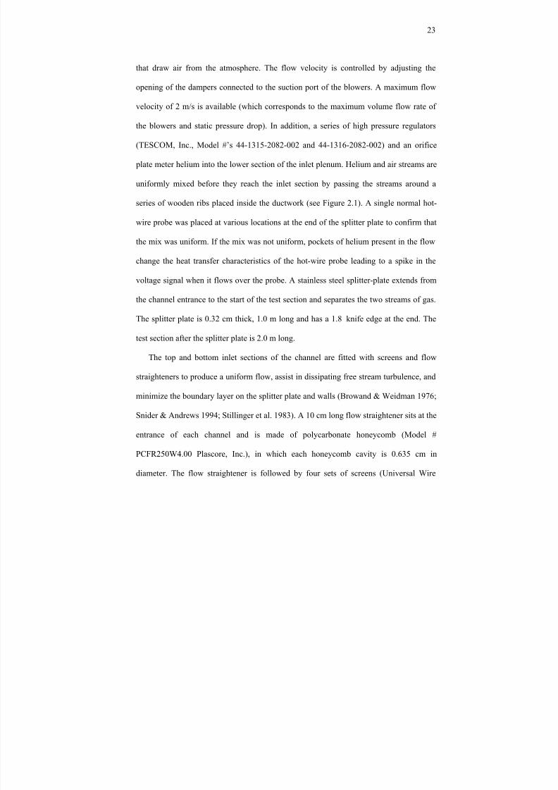
that draw air from the atmosphere. The flow velocity is controlled by adjusting the
opening of the dampers connected to the suction port of the blowers. A maximum flow
velocity of 2 m/s is available (which corresponds to the maximum volume flow rate of
the blowers and static pressure drop). In addition, a series of high pressure regulators
(TESCOM, Inc., Model #’s 44-1315-2082-002 and 44-1316-2082-002) and an orifice
plate meter helium into the lower section of the inlet plenum. Helium and air streams are
uniformly mixed before they reach the inlet section by passing the streams around a
series of wooden ribs placed inside the ductwork (see Figure 2.1). A single normal hot-
wire probe was placed at various locations at the end of the splitter plate to confirm that
the mix was uniform. If the mix was not uniform, pockets of helium present in the flow
change the heat transfer characteristics of the hot-wire probe leading to a spike in the
voltage signal when it flows over the probe. A stainless steel splitter-plate extends from
the channel entrance to the start of the test section and separates the two streams of gas.
The splitter plate is 0.32 cm thick, 1.0 m long and has a 1.8˚
knife edge at the end. The
test section after the splitter plate is 2.0 m long.
The top and bottom inlet sections of the channel are fitted with screens and flow
straighteners to produce a uniform flow, assist in dissipating free stream turbulence, and
minimize the boundary layer on the splitter plate and walls (Browand & Weidman 1976;
Snider & Andrews 1994; Stillinger et al. 1983). A 10 cm long flow straightener sits at the
entrance of each channel and is made of polycarbonate honeycomb (Model #
PCFR250W4.00 Plascore, Inc.), in which each honeycomb cavity is 0.635 cm in
diameter. The flow straightener is followed by four sets of screens (Universal Wire

8/3/2019 Arindam Banerjee- Statistically Steady Measurements of Rayleigh-Taylor Mixing in a Gas Channel
http://slidepdf.com/reader/full/arindam-banerjee-statistically-steady-measurements-of-rayleigh-taylor-mixing 38/198
24
Cloth, Inc.), one 30 × 30 mesh (wire/inch) with a wire diameter of 0.034 cm (37.1% free
area) followed by three 30 × 30 meshes (wire/inch) with a 0.0216 cm wire diameter
(55.4% free area). A full channel screen is placed at the end of the splitter plate as it is
found to be effective in minimizing the wake from the splitter plate (Koop 1976). This
end screen consists of a 22 × 22 mesh (wire/inch) with a 0.033 cm wire diameter and has
a free area of 49.8% (see Table 2.1). The honeycomb and meshes are placed sufficiently
upstream to dissipate any free stream turbulence (Tan-Atichat et al. 1982). The free area
chosen was consistent with turbulence management recommendations for wind tunnels
(Loehrke & Nagib 1972).
The velocities of the two streams were set so that there was no shear between the
flows ( mmixtureair U U U == ). This was ensured by introducing puffs of smoke in both the
top and bottom sections of the channel through small holes on bottom and top and
checking for shear. When at no shear, since the cross sectional area ( A) of the top and
bottom sections was identical, the volumetric flow rate of air and helium- air mixture in
the top and bottom channels respectively were equal. The mixture flow rate in the
bottom section of the channel was then given by:
AU m
V V V V m
He
He
air Heair bottom =+=+=
•••••
ρ (2.1)
The density of the helium-air mixture depends on the mass flow rate of Helium ( Hem& )
and the velocity of the two streams (U BmB) as:
⎥⎦
⎤⎢⎣
⎡−+=
He
air
m
Heair
bottom
mix AU
m
ρ
ρ ρ ρ 1
&(2.2)

8/3/2019 Arindam Banerjee- Statistically Steady Measurements of Rayleigh-Taylor Mixing in a Gas Channel
http://slidepdf.com/reader/full/arindam-banerjee-statistically-steady-measurements-of-rayleigh-taylor-mixing 39/198
25
TABLE 2.1 List of flow-straighteners and meshes in the inlet section of the facility(Note: for the location of each of these screens, see Figure 2.1)
Mesh Size Wire Diameter % Open Area Location Quantity
30 × 30 0.0340 cm 37.1 % A 1
30 × 30 0.0216 cm 55.4 % B 3
22 × 22 0.0330 cm 49.8 % C 1

8/3/2019 Arindam Banerjee- Statistically Steady Measurements of Rayleigh-Taylor Mixing in a Gas Channel
http://slidepdf.com/reader/full/arindam-banerjee-statistically-steady-measurements-of-rayleigh-taylor-mixing 40/198
26
The Atwood Number of the mix was hence given by:
AU
m
AU
m
A
m
He
He
air air
m
He
He
air
bottom
mixair
bottom
mixair t &
&
⎥⎦
⎤⎢⎣
⎡−+
⎥
⎦
⎤⎢
⎣
⎡−
=+
−=
ρ
ρ ρ
ρ
ρ
ρ ρ
ρ ρ
12
1
)(
)((2.3)
Since the mass flow rate of helium ( Hem& ) was needed to evaluate the Atwood number in
Equation 2.3, an accurate measurement of the helium mass flow rate was required.
Furthermore, air ρ and He ρ were dependent on the fluid temperatures. Thus, to get an
accurate estimate of the Atwood number, the densities of air and helium were obtained
from equations of state for the gases (see Appendix C).
2.2 Mass Flow Rate Calibration
Initial consideration was given to using a commercial gas flow meter or controller.
However, for the range of pressures (~ 2100 psig) and mass-flow rates being used (~0.1
lbm/s), such flow meters are expensive and complex. Furthermore, calibration data
obtained from the manufacturers are based on air and use of empirical laws to
compensate for the effects of Helium meant that the flow meters would require re-
calibration. Thus, it was decided to use a volumetric method at constant outlet pressure
for flow metering, in which, the gas was delivered from a supply, having passed through
an orifice (Jitschin et al. 1995). The main feature of the current set-up is the use of a thin
orifice for flow constriction and metering. The pressure drop across the orifice is
maintained so that the pressure ratio between the downstream and upstream locations is
below the critical pressure ratio. Hence, the flow is choked at the orifice and thus,

8/3/2019 Arindam Banerjee- Statistically Steady Measurements of Rayleigh-Taylor Mixing in a Gas Channel
http://slidepdf.com/reader/full/arindam-banerjee-statistically-steady-measurements-of-rayleigh-taylor-mixing 41/198
27
Figure 2.2 Schematic of flow metering unit for a constant mass flow rate of helium( R1: Regulator 1: 0-1500 psig; R2: Regulator 2: 0-1000 psig).
To Gas Channel
R1 R2 Orifice Flow
Plate ControlValve
From HeliumSupply
Flow MeteringUnit
PressureGauges

8/3/2019 Arindam Banerjee- Statistically Steady Measurements of Rayleigh-Taylor Mixing in a Gas Channel
http://slidepdf.com/reader/full/arindam-banerjee-statistically-steady-measurements-of-rayleigh-taylor-mixing 42/198
28
Figure 2.3 Calibration of mass flow rate of helium for different Atwood numbers. Themeasurement uncertainty of digital scale is ± 0.01 lbs. (Note: For the mass flow rate
calibration corresponding to an Atwood # 0.25, 2 bottles of helium were used for calibration. So the actual mass flow rate was twice the slope.)

8/3/2019 Arindam Banerjee- Statistically Steady Measurements of Rayleigh-Taylor Mixing in a Gas Channel
http://slidepdf.com/reader/full/arindam-banerjee-statistically-steady-measurements-of-rayleigh-taylor-mixing 43/198
29
TABLE 2.2 Calibrated mass flow rates for different orifice (Note: The measurementuncertainty of digital scale is ± 0.01 lbs. For the uncertainty in the measured Atwood
number, see Appendix B.3)
Mass Flow Rate (lbm/s)
No. of units
Diameter of
Orifice (inch) Experimental Theory
Atwood
Number
0.032 0.0066 ± 0.00007 0.0072 ~ 0.041
0.061 0.0234 ± 0.00007 0.0267 ~ 0.10
0.072 0.0284 ± 0.00014 0.0339 ~ 0.22
0.110 0.0507 ± 0.00014 0.0793 ~ 0.31
0.150 0.0654 ± 0.00014 0.1437 ~ 0.38
0.180 0.0825 ± 0.00014 0.2365 ~ 0.47
2
0.225TP
1PT 0.1350 ± 0.00014 0.3316 ~ 0.72
TP
1PT At this orifice size, the flow rates were extremely high. These flow rates were near the limit that the
TESCOM regulators can handle. It was recommended to branch the Helium metering system to at least 3units so that the effective flow rate through each regulator was reduced.
8/3/2019 Arindam Banerjee- Statistically Steady Measurements of Rayleigh-Taylor Mixing in a Gas Channel
http://slidepdf.com/reader/full/arindam-banerjee-statistically-steady-measurements-of-rayleigh-taylor-mixing 44/198
30
the mass flow rate through it was determined based on empirical relations (Wu &
Molinas 2001). To this end, the mass flow rate was measured by placing helium bottle(s)
on a sensitive digital scale (± 0.01 lbs) and recording the change in weight of the bottle
with time.
Figure 2.2 shows a schematic of the setup used for controlling and metering the mass
flow rate of helium into the gas channel. Two high pressure regulators, R1 and R2
(TESCOM, Inc.), are used to control the pressure drop from a supply pressure of ~2100
psig to the ambient pressure inside the channel. Two high pressure gauges (Swagelock,
Inc.) are connected as shown in the schematic to accurately read the pressure in the line
at two different downstream locations to ensure that the flow chokes at the orifice and
not at either of the regulators. Flexible ½” diameter stainless steel tubing is used to
connect all components. An orifice plate is placed after the downstream pressure gauge
and held in position by the flow control valve. Initially, the flow control valve is closed
and the pressure regulators are adjusted: the upstream regulator is fixed at 1050 psig to
ensure that the pressure ratio across R1 exceeds the critical pressure ratio and thus the
flow is not choked at R1; and the downstream pressure regulator R2 is set at 550 psig to
ensure the flow is not choked at R2. Thus, when the flow control valve is opened, the
flow is immediately choked at the orifice and a constant mass flow rate of helium until
the pressure in the bottles dropped below the set pressure (550 psig in this case). Table
2.2 shows the results of the mass flow rate calibrations for different orifices of diameters.
The theoretical mass flow rate was calculated based on equations for sub-critical flow
through the orifice (John 1984).
8/3/2019 Arindam Banerjee- Statistically Steady Measurements of Rayleigh-Taylor Mixing in a Gas Channel
http://slidepdf.com/reader/full/arindam-banerjee-statistically-steady-measurements-of-rayleigh-taylor-mixing 45/198
31
Figure 2.3 shows the mass flow rates of helium measured on the digital scale with
three different orifices. A straight line fit was performed through the data points obtained
and the mass flow rates were tabulated. The RP
2P
values for the fit in these cases vary
between 0.9992 and 0.9998. The Atwood number range given in Table 2.2 was
calculated based on the experimental mass flow rate for a given mean velocity (to
achieve the parabolic approximation). This facility arrangement empties 90% of the
Helium tanks at constant mass flow rate before the threshold of 550 psig is reached.
However, for the higher mass flow rates required for the high Atwood runs ( ABtB ≥ 0.5), the
flow rates exceed the maximum flow rates that can be accommodated by the regulators.
Hence, two helium metering units were connected in parallel to accommodate the higher
flow rate demands. Thus for ABtB ≥ 0.25, both the systems are used in parallel to give larger
run times for the experiment. A Kline McClintock uncertainty analysis (1953) was
performed to calculate the uncertainty in the Atwood number for the experiment and is
provided in Appendix B. The Atwood number range tabulated below was calculated
based on the experimental mass flow rate and varying the angle of spread in the mix
between 10º - 15º.
8/3/2019 Arindam Banerjee- Statistically Steady Measurements of Rayleigh-Taylor Mixing in a Gas Channel
http://slidepdf.com/reader/full/arindam-banerjee-statistically-steady-measurements-of-rayleigh-taylor-mixing 46/198
32
3. VISUALIZATION DIAGNOSTICS TP
∗PT
3.1 Visualization Technique – Calibration
The lighter fluid (air-helium mixture at the bottom) was colored with dark green
smoke (RC105G, Regin HVAC Products) to visualize the mixing layer. A row of 35
fluorescent lamps backlit the entire channel test section while Matte (frosted) Acetate
paper (MisterArt.com) serves as the white background and helped diffuse the light. Each
experiment was photographed using a Canon Powershot A80 digital camera. The digital
camera stored the pictures in JPEG format. Pictures were captured continuously at the
rate of 80 images per minute. The camera settings were manually chosen to eliminate
variations between images. Before the experiment was run, the shutter speed, aperture
and ISO settings were set so that it did not change during a run. The values used for
different Atwood number runs were given in Table 3.1. A manual focus was also used so
that the camera did not try to auto-focus on moving structures during the experiment.
The images were then cropped at the same location using a marker near the exit plenum
so that the mix width spanned the entire width of the image. The images were processed
and analyzed using MATLABP
©P. The relation between concentration and pixel intensity
was determined by using a calibration wedge. A calibration wedge is a triangular Plexi-
glass container filled with the same green smoke. The wedge has a depth (a) of 22
inches, width (b) of 24 inches and height (c) of 6 inches. It was found from a wedge
TP
∗PT Parts of this section including Figures 3.1, 3.2, 3.3, 3.4 and 3.5 have been reprinted with permission from
Banerjee A, Andrews MJ. 2006. Statistically steady measurements of Rayleigh-Taylor mixing in a gaschannel. Phys. Fluids 18:1-13

8/3/2019 Arindam Banerjee- Statistically Steady Measurements of Rayleigh-Taylor Mixing in a Gas Channel
http://slidepdf.com/reader/full/arindam-banerjee-statistically-steady-measurements-of-rayleigh-taylor-mixing 47/198
33
TABLE 3.1 Camera (Canon Powershot A80) settings at different Atwood numbers
(Note: For measurement uncertainties of Atwood number and mean velocity, seeAppendix B).
Atwood Number U BmB (m/s) Shutter Speed Aperture ISO
0.035 0.6 1/100 s F/8.0 50
0.259 1.2 1/100 s F/8.0 100

8/3/2019 Arindam Banerjee- Statistically Steady Measurements of Rayleigh-Taylor Mixing in a Gas Channel
http://slidepdf.com/reader/full/arindam-banerjee-statistically-steady-measurements-of-rayleigh-taylor-mixing 48/198
34
Figure 3.1 Intensity as a function of height for calibration wedge (Inset shows actualcalibration image) [wedge dimensions: a (depth) = 22 inches, b (width) = 24 inches, c
(height) = 6 inches)].
8/3/2019 Arindam Banerjee- Statistically Steady Measurements of Rayleigh-Taylor Mixing in a Gas Channel
http://slidepdf.com/reader/full/arindam-banerjee-statistically-steady-measurements-of-rayleigh-taylor-mixing 49/198
35
calibration (Banerjee & Andrews 2006; Snider & Andrews 1994) that the concentration
of smoke must be kept low to maintain a linear relation between the concentration and
measured intensity. Figure 3.1 shows that the camera response was linear for a dynamic
range over 100 pixel intensity values. For grayscale values less that 80 (lower means
darker), it was found the camera response became non-linear. Thus, care was taken to
ensure that the calibrated linear dynamic range from 100 to 200 was used during an
experimental run.
3.2 Correction for Non-Uniform Backlight
Extinction of light from source I BoB across the path z is given by Beer Lambert’s Law,
where κ is the monochromatic extinction coefficient (see Equation 3.1). Expanding the
exponential in a series and retaining the first term gives a linear relationship between the
applied and transmitted intensities along path z .
( )ω κ κ −=⎥⎦
⎤
⎢⎣
⎡
−≈⎟⎟ ⎠
⎞
⎜⎜⎝
⎛
−= ∫ ∫ 11exp),( 0
0
0
0
0 I dz I dz I y x I
z z
m (3.1)
where, ω ∫ = z
dz 0
κ is the absolute extinction coefficient of the medium. For this
experiment, the extinction coefficient is a function of the volumetric concentration of
smoke and the optical path length of light traveled. The calibration (Figure 3.1) shows
that this approximation is valid from 0 – 60% extinction of the light.
In an ideal experiment, the test section is irradiated with a uniform backlight, and
then any two points in the image with the same intensity is a result of an identical
attenuation of light. Using a linear relationship between the smoke concentration and

8/3/2019 Arindam Banerjee- Statistically Steady Measurements of Rayleigh-Taylor Mixing in a Gas Channel
http://slidepdf.com/reader/full/arindam-banerjee-statistically-steady-measurements-of-rayleigh-taylor-mixing 50/198
36
intensity, the concentration of the flow field can be defined from the intensity
distribution. The images of the channel during the run were found to be bright at the
center of the photograph and darker towards the edges. On first look, this effect may be
misinterpreted as optical vignetting. A photograph or drawing whose edges gradually
fade into the surrounding paper is called a vignette (Smith 2000). Most lenses exhibit
optical vignetting to some degree. The effect is strongest when the lens is used at wide
open apertures. Thus, the effect of vignetting was avoided by using a smaller aperture
(see Table 3.1). The gradual darkening of the edges was an effect on the non-uniform
light intensity of the fluorescent tubes which were bright at the center and darker
towards the edges. So, a background image (see Figure 3.2) was used to correct for non-
uniformities in the background intensity to a uniform intensity.
The background image was taken from a photograph of the test section without the
smoke. The present work used the method of Snider and Andrews (1994, 1995) for
correcting the linear intensity to extinction approximation. The corrected measured
intensity I Bcorr B that would exist if the background intensity was uniform ( uniform
o I ) can be
written as:
( )ω −= 10
uniform
corr I I (3.2)
Since ω is a function of the depth of the channel, it can be determined from the measured
intensity I Bm
Band the background intensity I B0
B. Thus, eliminating ω between Equations 3.1
and 3.2 gives:
m
uniform
corr I I
I I
0
0= (3.3)

8/3/2019 Arindam Banerjee- Statistically Steady Measurements of Rayleigh-Taylor Mixing in a Gas Channel
http://slidepdf.com/reader/full/arindam-banerjee-statistically-steady-measurements-of-rayleigh-taylor-mixing 51/198
37
Figure 3.2 Histogram for raw image.

8/3/2019 Arindam Banerjee- Statistically Steady Measurements of Rayleigh-Taylor Mixing in a Gas Channel
http://slidepdf.com/reader/full/arindam-banerjee-statistically-steady-measurements-of-rayleigh-taylor-mixing 52/198
38
Figure 3.3 Histogram for processed image.

8/3/2019 Arindam Banerjee- Statistically Steady Measurements of Rayleigh-Taylor Mixing in a Gas Channel
http://slidepdf.com/reader/full/arindam-banerjee-statistically-steady-measurements-of-rayleigh-taylor-mixing 53/198
39
The corrected intensity, I Bcorr B, is the intensity that would exist if the backlighting is
uniform and takes into account the actual background intensity and the measured
intensity for each pixel. The peak value of a histogram of the background image was
selected as uniform I 0 . Figures 3.2 and 3.3 shows the intensity population before and after
adjusting for non-uniform backlighting. In Figure 3.2, the peaks correspond to regions at
the edge or outside the mix, and were thus more prone to non-uniformity in backlighting.
The correction for non-uniform backlighting gives narrower peaks for pixel populations
at low and high intensities, which correspond to regions where the concentrations were
0% and 100%. This shows the improvement obtained with the backlighting correction,
as these were the regions at the periphery of the mix region where the non-uniformity in
backlighting was more pronounced.
3.3 Steps in Image Processing Diagnostics
The following steps were followed to capture images of the channel before and
during an experimental run:
• Fix digital camera settings manually (refer to Table 3.1). Check image
histogram to ensure that the peaks were within the linear range of calibration.
• Take background image before and after completion of run.
• Run channel and take pictures in “continuous-burst” mode.
Once the run was completed, the images were transferred from the camera memory to a
PC. To process the background images, the following steps were adopted:
• Process the background images and store an averaged background image.

8/3/2019 Arindam Banerjee- Statistically Steady Measurements of Rayleigh-Taylor Mixing in a Gas Channel
http://slidepdf.com/reader/full/arindam-banerjee-statistically-steady-measurements-of-rayleigh-taylor-mixing 54/198
40
• Locate 3 physical points on the averaged background image and crop image.
If the image was tilted, rotate background image. Pick an origin in the image.
Pick 2 locations on the image of known distance to calculate physical
distance per pixel.
• Check histogram of background image and find the pixel intensity value
corresponding to the peak of the histogram. Denote this value as uniform
o I in
the background correction (see Equation 3.3).
• Store processed background image.
Once the background Image has been processed and stored, the images taken during the
run were first converted to grayscale and then processed as follows:
• Average all images during the run. Locate 3 physical points on the averaged
image and crop image. If the image was tilted, rotate the image.
• Check histogram of averaged image.
• Perform background correction based on Equation 3.3.
• Check histogram of corrected image.
• Store processed average image.
This averaged image can be used for drawing fraction profiles; image contours as well as
computing the mix widths and the growth constant α for the experimental run (see
Section 6).

8/3/2019 Arindam Banerjee- Statistically Steady Measurements of Rayleigh-Taylor Mixing in a Gas Channel
http://slidepdf.com/reader/full/arindam-banerjee-statistically-steady-measurements-of-rayleigh-taylor-mixing 55/198
41
3.4 Qualitative Measurements
Figures 3.4 a-b show photographs of experimental runs at Atwood numbers of 0.04
(U BmB = 0.5 m/s) and 0.097 (U BmB = 0.85 m/s). Two gas streams, one containing pure air (top
half) and the other consisting of air-helium mixture colored with green smoke (bottom
half), flow parallel to the splitter plate. The photograph shows the formation and
evolution of buoyancy driven mixing layer. As described previously, care was taken to
ensure that there was no shear between the two streams. Figures 3.2 and 3.3 show a lack
of fluctuations or variation of smoke outside the mixing layer. This indicates that large
scale plumes and small disturbances were confined to the mixing layer. This behavior
was common in plane shear flow where turbulence was associated with shearing of the
stream-wise flow (Brown & Roshko 1974; Tennekes & Lumley 1994) and was also
apparent in the present buoyancy driven flow. The mixing process observed is one of
engulfment of air-helium from below and air from above. This resulted in a mix region,
whose height increased with downstream distance. Figures 3.5 a-b, are close up views of
the mix, and show that that the buoyant mixing layer grows as a front of rising and
falling plumes (“bubble and spikes”). Multiple plumes form span-wise across the
channel. Vortices form around the edge of the mushroom head of light or heavy fluid as
they penetrate through each other. Four major structures are observed at regular
frequency along the stream-wise direction (right to left). The last two structures in the
series (extreme left) are seen to pair. The pictures show that an advanced plume (extreme
left) pairs with an earlier plume (second from left). Such “bubble competition” is
observed throughout the length of the mix.

8/3/2019 Arindam Banerjee- Statistically Steady Measurements of Rayleigh-Taylor Mixing in a Gas Channel
http://slidepdf.com/reader/full/arindam-banerjee-statistically-steady-measurements-of-rayleigh-taylor-mixing 56/198
42
(a)
(b)
Figure 3.4 View of the mixing process in the channel at (a) ABtB # 0.04 (U BmB = 50 cm/s) and(b) ABtB # 0.097 (U BmB = 85 cm/s).

8/3/2019 Arindam Banerjee- Statistically Steady Measurements of Rayleigh-Taylor Mixing in a Gas Channel
http://slidepdf.com/reader/full/arindam-banerjee-statistically-steady-measurements-of-rayleigh-taylor-mixing 57/198
43
(a)
(b)
Figure 3.5 Close-up view of the three dimensional plumes across the channel for (a) ABtB #0.04 (U BmB = 50 cm/s) and (b) ABtB # 0.097 (U BmB = 85 cm/s).

8/3/2019 Arindam Banerjee- Statistically Steady Measurements of Rayleigh-Taylor Mixing in a Gas Channel
http://slidepdf.com/reader/full/arindam-banerjee-statistically-steady-measurements-of-rayleigh-taylor-mixing 58/198
44
Figure 3.6 Movie of the mixing process for ABtB # 0.259 (U BmB = 1.2 m/s).

8/3/2019 Arindam Banerjee- Statistically Steady Measurements of Rayleigh-Taylor Mixing in a Gas Channel
http://slidepdf.com/reader/full/arindam-banerjee-statistically-steady-measurements-of-rayleigh-taylor-mixing 59/198
45
4. HOT-WIRE DIAGNOSTICS
Velocity measurements were made using a hot-wire Probe of diameter 5 µm
(single wire: 55P16) coupled to a Constant Temperature Anemometer (CTA) unit (Mini-
CTA, Dantec Dynamics). Temperature measurements were made using the Single
Normal (SN) wire probes (55P16) as cold wire probes coupled to a Constant Current
Anemometer unit (A.A. Laboratories, Inc.). Although our use of CTA and CCA was
typical, we briefly review its application to measurement of our R-T mix, and note
refinements and differences from the typical set up.
4.1 Constant Temperature Anemometry (CTA) for Measuring Velocity Fluctuations
The CTA unit is an analog instrument designed for measuring velocity in gases and
works on the basis of convective heat transfer from a heated sensor to the surrounding
fluid, the heat transfer being primarily related to the fluid velocity. The CTA is suited for
measurement of fast gas velocity fluctuations of fine scales and high frequencies
(Jørgensen 1996). The complete measuring system used in the present study consists of
(a) Single Normal Hot-wire probe (SN probe: 55P16) with support and 4-m BNC-BNC
probe cable, (b) Mini-CTA anemometer (54T30) with built-in signal conditioner and
power adapter, (c) SC 2040 Sample and Hold Board (National Instruments) connected to
a PCI-MIO-16E-4 A/D board (National Instruments) mounted in a Pentium 4 computer.
NI-DAQ driver software and Lab-View DAQ Software are used for data collection at
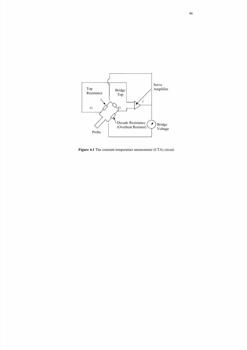
8/3/2019 Arindam Banerjee- Statistically Steady Measurements of Rayleigh-Taylor Mixing in a Gas Channel
http://slidepdf.com/reader/full/arindam-banerjee-statistically-steady-measurements-of-rayleigh-taylor-mixing 60/198
46
Figure 4.1 The constant temperature anemometer (CTA) circuit.
Probe
BridgeVoltage
ServoAmplifier
Decade Resistance(Overheat Resistor)
Top
Resistance
Bridge
Top
eB2B
eB1B
i

8/3/2019 Arindam Banerjee- Statistically Steady Measurements of Rayleigh-Taylor Mixing in a Gas Channel
http://slidepdf.com/reader/full/arindam-banerjee-statistically-steady-measurements-of-rayleigh-taylor-mixing 61/198
47
TABLE 4.1 Sample operating parameters for SN wire coupled to a mini-CTA unit(overheat ratio = 1.6)
Probe specific parameters.
Sensor resistance, RB20B 3.49 Ω
Sensor lead resist., RBLB 0.9 Ω
Support resistance, RBsB 0.44 Ω
Cable resistance, RBcB 0.2 Ω
Sensor TCR, α B20B 0.0036 /K
Wire operating parameters
Desired wire temp., T BwB 191.43 °C
Operating resistance, RBwB 5.64 Ω
Total resistance, RB
TB
7.18 ΩDecade resistance, RBDB 142.48 Ω
Bridge ratio, M 1:20
Overheat ratio, a (= RBwB/ RBaB) 1.6

8/3/2019 Arindam Banerjee- Statistically Steady Measurements of Rayleigh-Taylor Mixing in a Gas Channel
http://slidepdf.com/reader/full/arindam-banerjee-statistically-steady-measurements-of-rayleigh-taylor-mixing 62/198
48
desired frequencies. Figure 4.1 shows the CTA circuit that was used. A hot-wire probe
was placed in a Wheatstone bridge. As the flow conditions vary, the error voltage eB2 B – eB1B
is a measure of the corresponding change in the wire resistance. These two voltages form
the input to the operational servo amplifier. The selected amplifier has an output current,
i, which is inversely proportional to the resistance change of the hot-wire sensor. Feeding
this current back to the top of the bridge restores the sensor’s resistance to its original
value. Modern amplifiers used in anemometers have a very fast response time (~ 450
kHz). Furthermore, in the CT mode, the sensor is maintained at a constant temperature
except for very high frequency fluctuations. The CTA circuit operates on a bridge ratio
of 1:20 and has a frequency response of 10 kHz (3 dB limit). Various CTA and probe
parameters used are listed in Table 4.1. A 55P16 single normal probe was used for all
the single wire measurements. Various parameters given in Table 4.1 correspond to
specifications for the SN probe (Dantec Dynamics), wherein the overheat ratio
determines the working temperature (T B
wireB
) of the sensor. An overheat adjustment is
based on the measured wire resistance at the ambient fluid temperature. The probe-CTA
combination used during calibration was also not changed during the run to preserve the
calibration. A variation as large as 25% in the bridge voltage was obtained if the probe-
circuit combination was altered.
4.1.1 Calibration of a Single-Normal Hot-Wire Probe
A calibration was performed to establish the relation between CTA output and flow
velocity by exposing the probe to a set of known velocities, U , and then recording the
voltages, E . A curve fit through the points ( E , U ) gives the transfer function for

8/3/2019 Arindam Banerjee- Statistically Steady Measurements of Rayleigh-Taylor Mixing in a Gas Channel
http://slidepdf.com/reader/full/arindam-banerjee-statistically-steady-measurements-of-rayleigh-taylor-mixing 63/198
49
converting data records from voltages into velocities. Due to individual features of each
probe, variations in anemometer circuits and settings; and variations in the flow
temperature, the hot-wire calibration may change. The calibration was thus checked at
regular intervals and was re-performed if necessary. As a quick check before an
experiment, a reference voltage reading was recorded by placing the probe in a known
fluid velocity. The temperature of the flow as well as the ambient room temperature was
logged. This was done to ensure that the reference point (voltage reading) during the test
run matched with the calibration. Typically, calibration was either carried out in a
dedicated probe calibrator or in a wind tunnel with a pitot-static tube as the velocity
reference (Bruun 1996; Bruun & Tropea 1985; Saddoughi & Veeravalli 1996). The
velocity was evaluated from a difference in the pressure reading, ∆ P , across the pitot
static tube or a calibration nozzle. However at low speeds (≤ 3 m/s), the value of ∆ P in
air becomes small (< 1 mm of water) and it was difficult to obtain accurate estimates of
velocities by this method.
For the present study, a separate jet-flow calibration was used as shown in Figure
4.2. Similar methods has been used before in a number of investigations (Almquist &
Legath 1965; Andrews et al. 1972; Koppius & Trines 1976; Lee & Budwig 1991; Manca
et al. 1988). A pressure regulator was used to control the supply from the compressed air
line (~ 100 psig). The air supply was fed to a proportioner meter (Model # P21A1-BA2,
Aalborg Corp.) which could control air flow rates upto 60 L/min. A 1/2” diameter PVC
pipe was used to create a jet. The hot-wire was inserted towards the rear end so that it
was well within the fully developed velocity profile. The temperature was

8/3/2019 Arindam Banerjee- Statistically Steady Measurements of Rayleigh-Taylor Mixing in a Gas Channel
http://slidepdf.com/reader/full/arindam-banerjee-statistically-steady-measurements-of-rayleigh-taylor-mixing 64/198
50
Figure 4.2 Schematic of setup used for hot-wire calibration.
CompressedAir Flow
Controlvalve
Hot-wire probe
Regulator
Air Proportioner Meter
HeliumSupply
Mixing Section
Test Section

8/3/2019 Arindam Banerjee- Statistically Steady Measurements of Rayleigh-Taylor Mixing in a Gas Channel
http://slidepdf.com/reader/full/arindam-banerjee-statistically-steady-measurements-of-rayleigh-taylor-mixing 65/198
51
also recorded during calibration (Betti et al. 2001) by using a E-type thermocouple.
Later, during the experiment, if the mean temperature of the flow (T BfluidB) during the
experiment varied from the temperature during calibration, the CTA data records were
corrected for temperature variations using Equation 4.1 (Kanevce & Oka 1973).
a
calibwire
fluid wire
corr E T T
T T E ⋅⎟⎟
⎠
⎞⎜⎜⎝
⎛
−
−=
5.0
(4.1)
4.1.2 Hot-Wire Calibration Equations
In selecting the hot-wire response equation, we faced dual objectives of high
accuracy and ease of use. Based on historical and physical considerations, we considered
using a polynomial curve fit in the form )( E F U = or a more traditional relationship
from the original investigation by King (1914) which assumed a form )(U F E = .
(a) Polynomial curve fits: A 4th order polynomial plot was fitted to this data and
found to have a RP
2P value of 0.9999. Errors associated with the 4th order fit in Figure 4b
can be attributed to errors in velocity measurement inside the gas channel. For
comparison purposes, the goodness of fit of the selected hot-wire response equation was
described by the related normalized standard deviation, ε Bu,B which was defined as:
2
1
1
2
11
⎥⎥⎦
⎤
⎢⎢⎣
⎡⎟⎟ ⎠
⎞⎜⎜⎝
⎛ −= ∑
=
N
i calib
uU
U
N ε (4.2)
The value of ε BuB was tabulated in Table 4.2 for polynomial fits of order 2 - 4.
(b) King’s Law Fits: The relationship between voltage and velocity was often
assumed to be of the form:
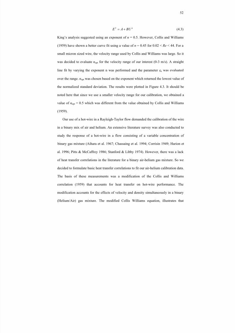
8/3/2019 Arindam Banerjee- Statistically Steady Measurements of Rayleigh-Taylor Mixing in a Gas Channel
http://slidepdf.com/reader/full/arindam-banerjee-statistically-steady-measurements-of-rayleigh-taylor-mixing 66/198
52
n BU A E +=2 (4.3)
King’s analysis suggested using an exponent of n = 0.5. However, Collis and Williams
(1959) have shown a better curve fit using a value of n = 0.45 for 0.02 < Re < 44. For a
small micron sized wire, the velocity range used by Collis and Williams was large. So it
was decided to evaluate nBopt B for the velocity range of our interest (0-3 m/s). A straight
line fit by varying the exponent n was performed and the parameter ε BuB was evaluated
over the range. nBoptB was chosen based on the exponent which returned the lowest value of
the normalized standard deviation. The results were plotted in Figure 4.3. It should be
noted here that since we use a smaller velocity range for our calibration, we obtained a
value of nBopt B = 0.5 which was different from the value obtained by Collis and Williams
(1959).
Our use of a hot-wire in a Rayleigh-Taylor flow demanded the calibration of the wire
in a binary mix of air and helium. An extensive literature survey was also conducted to
study the response of a hot-wire in a flow consisting of a variable concentration of
binary gas mixture (Aihara et al. 1967; Chassaing et al. 1994; Corrisin 1949; Harion et
al. 1996; Pitts & McCaffrey 1986; Stanford & Libby 1974). However, there was a lack
of heat transfer correlations in the literature for a binary air-helium gas mixture. So we
decided to formulate basic heat transfer correlations to fit our air-helium calibration data.
The basis of these measurements was a modification of the Collis and Williams
correlation (1959) that accounts for heat transfer on hot-wire performance. The
modification accounts for the effects of velocity and density simultaneously in a binary
(Helium/Air) gas mixture. The modified Collis Williams equation, illustrates that

8/3/2019 Arindam Banerjee- Statistically Steady Measurements of Rayleigh-Taylor Mixing in a Gas Channel
http://slidepdf.com/reader/full/arindam-banerjee-statistically-steady-measurements-of-rayleigh-taylor-mixing 67/198
53
Figure 4.3 Variation in ε BuB (goodness of fit) with exponent in power law relationshipfrom SN wire calibration data in air at overheat ratio 0.6 over a velocity range of
0.2-3 m/s.
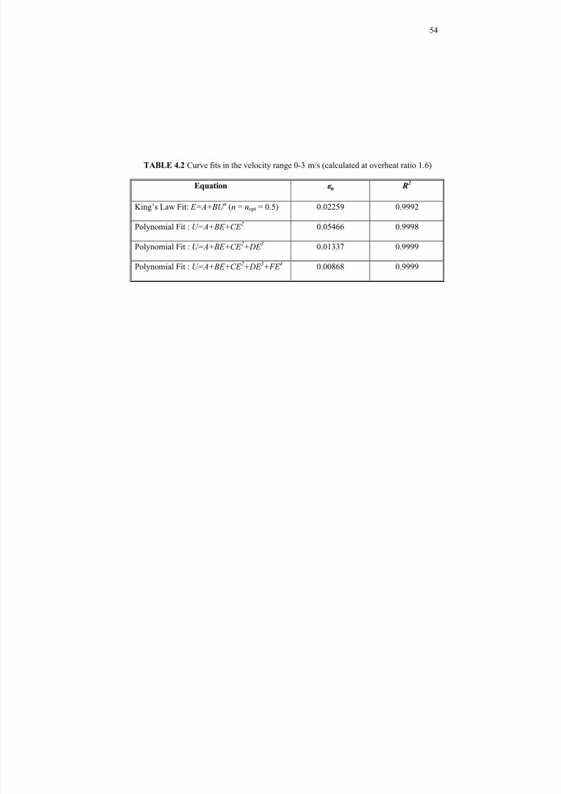
8/3/2019 Arindam Banerjee- Statistically Steady Measurements of Rayleigh-Taylor Mixing in a Gas Channel
http://slidepdf.com/reader/full/arindam-banerjee-statistically-steady-measurements-of-rayleigh-taylor-mixing 68/198
54
TABLE 4.2 Curve fits in the velocity range 0-3 m/s (calculated at overheat ratio 1.6)
Equation ε BuB RP
2P
King’s Law Fit: E=A+BU Pn
P (n = nBopt B = 0.5) 0.02259 0.9992
Polynomial Fit : U=A+BE+CE P2
P 0.05466 0.9998
Polynomial Fit : U=A+BE+CE P2
P+DE P3
P 0.01337 0.9999
Polynomial Fit : U=A+BE+CE P2
P+DE P3
P+FE P4
P 0.00868 0.9999

8/3/2019 Arindam Banerjee- Statistically Steady Measurements of Rayleigh-Taylor Mixing in a Gas Channel
http://slidepdf.com/reader/full/arindam-banerjee-statistically-steady-measurements-of-rayleigh-taylor-mixing 69/198
55
Figure 4.4 Hot-wire calibration data (King’s law fit) in air at overheat ratio 1.9(∆T =257.14˚C) and 1.6 (∆T =171.43˚C).

8/3/2019 Arindam Banerjee- Statistically Steady Measurements of Rayleigh-Taylor Mixing in a Gas Channel
http://slidepdf.com/reader/full/arindam-banerjee-statistically-steady-measurements-of-rayleigh-taylor-mixing 70/198
56
Figure 4.5 Variation in King’s Law constants for different volume fractions of helium ina binary air-helium mixture. The plots are for overheat Ratio 1.9 (∆T =257.14˚C) and 1.6(∆T =171.43˚C). (Note: The constants A, B were obtained from a linear fit of E P
2P vs. U P
0.5P
for a volume fraction range of φ = 0→1. RP
2P values for these fits range from 0.9930 to
0.9993. A representative calibration plot for E P2P vs. U P0.5P for air is provided in Figure 4.4)

8/3/2019 Arindam Banerjee- Statistically Steady Measurements of Rayleigh-Taylor Mixing in a Gas Channel
http://slidepdf.com/reader/full/arindam-banerjee-statistically-steady-measurements-of-rayleigh-taylor-mixing 71/198
57
the rate of heat transfer from the wire is dependent on the velocity as well as the
properties of the cooling fluid, and is written as:
( ) ( ) ( )[ ]45.033.02.017.0 RePr Pr 56.0Pr Pr 24.0 d air mixair mix fluid film T T Nu += (4.4)
where, Nu is the Nusselt number, T BfilmB is the average of the wire temperature (T BwireB) and
the fluid (mix) temperature ( fluid T ), ReBdB is the Reynolds number and Pr the Prandtl
number. All the properties were evaluated at T BfilmB. Thus a linear (King’s Law) fit was
applied to all calibration data as it was easy to use for formulating correlations of the
type described in Equation 4.4. Figure 4.4 shows a calibration plot in air at overheat ratio
1.9 and 1.6. It was seen that the response was fairly linear over the range of velocities
under consideration. Figure 4.5 plots the slope and intercept obtained from a King’s Law
fit as a function of the volume fraction of helium in a binary air-helium mixture. Details
about the heat transfer correlations can be found in section 5.
4.2 Constant Current Anemometry (CCA) for Measuring Temperature Fluctuations
4.2.1 The Need for a CCA Unit
In the present experiment, the density gradient needed to create a R-T Instability was
obtained by using a heavy fluid (air) over a light one (air-helium mixture). For the hot-
wire measurements, it was important to locate the position of the probe in the mix
(Banerjee & Andrews 2006; Mueschke 2004; Ramaprabhu & Andrews 2004; Wilson &
Andrews 2002). The addition of helium to the mix caused a small temperature gradient
(~2º C) along the vertical ( y) direction (i.e. from the air to the air/helium mixture). An
electric coil heater (1500W) was used to heat the air stream, thus creating an overall

8/3/2019 Arindam Banerjee- Statistically Steady Measurements of Rayleigh-Taylor Mixing in a Gas Channel
http://slidepdf.com/reader/full/arindam-banerjee-statistically-steady-measurements-of-rayleigh-taylor-mixing 72/198
58
gradient of ~4º C. We took advantage of this small temperature gradient and initially
used thermocouples to check for the centerline of the mix. The thermocouple
temperature diagnostics consisted of an E -type thermocouple (40 gauge wire of nickel-
chromium and constantan) that was positioned at different downstream locations in the
channel to ensure that the center line of the mix remains horizontal (Mueschke 2004;
Ramaprabhu & Andrews 2004; Wilson & Andrews 2002). However, the time response of
the E -type thermocouple was found ~ 20 Hz. So this was discontinued and a 5 µm SN
wire probe (Model #55P16) was used as a cold wire probe coupled to a Constant Current
Anemometer unit (A.A. Laboratories, Inc.). At the start of the experiment, the heater was
switched ON and the cold wire was placed close to the geometric centerline of the
mixing layer by visual inspection and the data was logged. The centerline offset factor φ
(as given in Equation 4.5) was computed after the logging process as:
1
1
−
⎥
⎥
⎦
⎤
⎢
⎢
⎣
⎡
⎟
⎟
⎠
⎞
⎜
⎜
⎝
⎛
−
−+=
topi
ibottom
top
bottom
top
p
bottom
p
T T
T T
C
C
ρ
ρ φ (4.5)
where, bottom
pC and bottomT were the specific heat and temperature of the helium-air mixture
(flow at the bottom section of the channel); top
pC and topT were the specific heat and
temperature of air (flow at the top section of the channel) ; and iT was the temperature of
the mix. If ≠φ 0.5, the position of the cold-wire was readjusted and the data logging
process repeated. The cold-wire position was adjusted until φ approaches a value of 0.5
with an accuracy of 5%. Once the centerline was found, the heater was switched OFF.
The hot-wire measurements were then taken at the determined location.

8/3/2019 Arindam Banerjee- Statistically Steady Measurements of Rayleigh-Taylor Mixing in a Gas Channel
http://slidepdf.com/reader/full/arindam-banerjee-statistically-steady-measurements-of-rayleigh-taylor-mixing 73/198
59
4.2.2 The Cold (Resistance) Wire Probe
Over a limited temperature range, the resistance of a wire can be approximated as a
linear function of temperature, i.e.,
( )[ ]201 2020 −+= wirewire T R R α (4.6a)
where RBwireB is the wire resistance at T BwireB, the wire temperature; RB20B and αB20B, the wire
resistance and the temperature coefficient of resistivity at a reference temperature of
20ºC. To maintain a linear relationship as depicted by Equation 4.6a, the reference
temperature should be chosen in the range of interest. The resistance RB20B is related to the
sensor dimensions, l BwireB (length of the wire) and d BwireB (wire diameter) based on the
relation:
42
2020
wire
wire
d
l R
π
σ = (4.6b)
The resistance fluctuations sensed by the wire as the fluid flows over it was
converted to voltage fluctuations by passing a small current, I , through the sensor. The
produced voltage fluctuations, e(t ), are related to the temperature fluctuations in the fluid
by the relation:
( ) [ ]202020 )( T t T IRt e wire −= α (4.7)
Measurement of low amplitude, small scale and high frequency temperature fluctuations
are important in turbulence research. Such measurements have been made possible by
use of low noise, high frequency AC Wheatstone bridges (LaRue et al. 1975). The
temperature calibration of a resistance-wire was used to determine the calibration
constants in the relationship as shown in Figure 4.6.

8/3/2019 Arindam Banerjee- Statistically Steady Measurements of Rayleigh-Taylor Mixing in a Gas Channel
http://slidepdf.com/reader/full/arindam-banerjee-statistically-steady-measurements-of-rayleigh-taylor-mixing 74/198
60
Figure 4.6 Calibration curve for cold wire (resistance wire) probe.

8/3/2019 Arindam Banerjee- Statistically Steady Measurements of Rayleigh-Taylor Mixing in a Gas Channel
http://slidepdf.com/reader/full/arindam-banerjee-statistically-steady-measurements-of-rayleigh-taylor-mixing 75/198
61
4.3 Single Wire Measurements
For the Rayleigh-Taylor mix experiments under consideration, velocity fluctuations
in all three mutually perpendicular directions are significant. When using a hot-wire
probe with a CTA unit, there are a number of methods by which the velocity fluctuations
can be resolved and measured accurately. One method uses a 3-wire probe to resolve all
3 components. However, besides the probe being expensive, the 3-wire method requires
an accurate calibration (velocity, density and directional) of the probe. An alternate
method resolves the three velocity components by using a multi-position single wire
technique (Bruun 1972). This method does not require complicated calibration and is
easy to implement. However, Bruun’s method does not incorporate density effects.
Measurements using this method is thus limited only to the low Atwood measurements
( ABt B~ 0.035) which contains less than 3.3% by volume. This was used as a first trial.
Errors associated with this assumption are described in Appendix B.7.1. A multi-
position multi-overheat (mpmo) single wire technique, which incorporates the effect of a
binary gas mixture of air and helium is used (Corrisin 1949; Kovasznay 1950). This
technique requires extensive calibration to take into account effects of density variation
in our flow. Both the techniques are described in details in the following sections.
4.3.1 Multi-position Single Wire Technique
H.H. Bruun (1972) used a multi-position single-wire technique by holding a SN wire
at different orientations to the flow to measure all the 3 velocity components. The
components were not measured simultaneously but by orienting the hot-wire (directions
given in Table 4.3) and ensuring that the probe was at the same spatial location . In his

8/3/2019 Arindam Banerjee- Statistically Steady Measurements of Rayleigh-Taylor Mixing in a Gas Channel
http://slidepdf.com/reader/full/arindam-banerjee-statistically-steady-measurements-of-rayleigh-taylor-mixing 76/198
62
analysis, Bruun used a flow that was two-dimensional ( 0=W ) with three dimensional
fluctuations. However, since the mean flow field used in the present experiment was
one-dimensional ( 0== W V ), the technique of Bruun reduced to three measurements
instead of the six roll positions required to resolve the two dimensional mean flow.
Following Bruun, the velocity vector V r
was taken to have the velocity
components ),,( wvuU ′′′+ . Taking into consideration a contribution from the angle of
incidence, the equations were resolved to determine the 3 different orientations as given
in Table 4.3. For a wire normal to the mean flow direction, with wire support parallel to
the flow (position 1), the mean component U BmB, is given by:
⎥⎥⎦
⎤
⎢⎢⎣
⎡ ′′+−
′′−
′+++=
3
2
22
2
2
2
2
21
2
21
2
11
U
wub
U
wu
U
W
U
wb
U
W U U m (4.8)
Since 0≈W and ignoring 3rd order terms, Equation 4.8 simplifies to the form for the
mean component of the flow as:
⎥⎥⎦
⎤
⎢⎢⎣
⎡ ′++=
2
2
2
211
U
wbU U m (4.9)
In Equations 4.8 and 4.9, ‘b’ is a constant of calibration for the probe and is calculated
from the following relation:
)sin1( 2 γ γ ⋅+=± bU U (4.10)
where U U ,γ ± are the velocities measured during calibration in air. The fluctuating
component measured by a hot-wire placed in position 1 (see Table 4.3 and Figure 4.7)
can be written as:
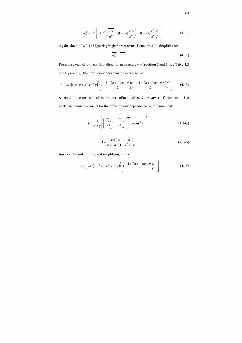
8/3/2019 Arindam Banerjee- Statistically Steady Measurements of Rayleigh-Taylor Mixing in a Gas Channel
http://slidepdf.com/reader/full/arindam-banerjee-statistically-steady-measurements-of-rayleigh-taylor-mixing 77/198
63
⎥⎥⎦
⎤
⎢⎢⎣
⎡
′
′′+−
′
′′++
′
′′+′=′
22
22
2
2
2
22 )21()21(21U u
wub
U u
wub
u
wu
U
W uum
(4.11)
Again, since 0≈W and ignoring higher order terms, Equation 4.11 simplifies to:
22 uum′=′ (4.12)
For a wire yawed to mean flow direction at an angle ± γ (position 2 and 3, see Table 4.3
and Figure 4.5), the mean component can be expressed as:
( )⎥⎥⎦
⎤
⎢⎢⎣
⎡ ′′++−
′++++=± 3
22
2
22
2
1222
2
tan21
2
tan211sincos
U
wu Ab
U
w Abk U U
γ γ γ γ γ
(4.13)
where b is the constant of calibration defined earlier, k the yaw coefficient and, A, a
coefficient which accounts for the effect of yaw dependence on measurements.
2
1
2
5.0
2
20
2
0
2
0
2
45cos
sin
1
⎥⎥⎥
⎦
⎤
⎢⎢⎢
⎣
⎡
−⎟⎟
⎠
⎞
⎜⎜
⎝
⎛
−
−=
==
=±=γ
γ γ
γ
U
U
E E
E E k
o
o
(4.14a)
222
22
)1(cos)1(cosk k
k A+−⋅
−⋅=α
α (4.14b)
Ignoring 3rd order terms, and simplifying, gives:
( )⎥⎥⎦
⎤
⎢⎢⎣
⎡ ′++++=± 2
22
2
1222
2
tan211sincos
U
w Abk U U
γ γ γ γ
(4.15)

8/3/2019 Arindam Banerjee- Statistically Steady Measurements of Rayleigh-Taylor Mixing in a Gas Channel
http://slidepdf.com/reader/full/arindam-banerjee-statistically-steady-measurements-of-rayleigh-taylor-mixing 78/198
64
Figure 4.7 Co-ordinate system for measurements and various orientations of hot-wireused for measurements (probe axis was normal to the dotted line).
Hot-wire
y
z
Hot-wire
x, U
y, v’
z, w’
Flow
γ : Yaw Angleδ : Roll Angle x
z

8/3/2019 Arindam Banerjee- Statistically Steady Measurements of Rayleigh-Taylor Mixing in a Gas Channel
http://slidepdf.com/reader/full/arindam-banerjee-statistically-steady-measurements-of-rayleigh-taylor-mixing 79/198
65
TABLE 4.3 Various measurement orientations for multi-position measurementtechnique. The measurement uncertainty of the positions is ± 2.5º
Position γ δ
1 0º 0 º
2 45º 90º
3 -45º 90º

8/3/2019 Arindam Banerjee- Statistically Steady Measurements of Rayleigh-Taylor Mixing in a Gas Channel
http://slidepdf.com/reader/full/arindam-banerjee-statistically-steady-measurements-of-rayleigh-taylor-mixing 80/198
66
In addition, the fluctuating component (ignoring 3rd and 4th order terms) can be written
as:
( ) vu Av Auk u ′′⋅′⋅+′+=′± γ γ γ γ γ tan2tansincos 22222222 m (4.16)
A value for 2v was obtained by adding Equations 4.16 for γ = +45˚ and - 45˚ to get:
( )( ) 22
222
45
2
452
1
1
Ak
uk uuv
+
′+−′+′=′ −+ (4.17)
Thus, using Equations 4.12, 4.15 and 4.17, the values of 22 ,vu ′′ and 2w′ can be
evaluated. The values of k and A were evaluated by performing a yaw-calibration for the
wire (Bruun 1972; Bruun & Tropea 1985).
4.3.2 Multi-position Multi-Overheat Single Wire Technique
The mean voltage across a wire oriented at an angle to the flow can be written as:
( ) ρ ,,, wvu f E = (4.18)
The total change in the mean voltage, E, due to change in the independent variables is:
ρ
ρ ρ
ρ
ρ ρ ρ
d edwedvedue
d E
dww
E dv
v
E du
u
E dE
wvU
wvuvuwuwv
∆+∆+∆+∆=
⎟⎟ ⎠
⎞⎜⎜⎝
⎛
∂∂
+⎟ ⎠
⎞⎜⎝
⎛ ∂∂
+⎟ ⎠
⎞⎜⎝
⎛ ∂∂
+⎟ ⎠
⎞⎜⎝
⎛ ∂∂
=,,,,,,,,
(4.19)
For small fluctuations in velocity and density, it was assumed that the wire fluctuation
can be written as (Rose 1973):
ρ
ρ ρ
′∆+
′∆+
′∆+
′∆=
′e
U
we
U
ve
U
ue
E
ewV U (4.20a)

8/3/2019 Arindam Banerjee- Statistically Steady Measurements of Rayleigh-Taylor Mixing in a Gas Channel
http://slidepdf.com/reader/full/arindam-banerjee-statistically-steady-measurements-of-rayleigh-taylor-mixing 81/198
67
The wire sensitivities are evaluated based on calibration of the wires and are defined as
follows:
0,,0,,
,,,,
,,,,
ln
1ln
lnln
=∆=∆
∆∆
∆∆
=∂
∂=∆
=∂
∂=∆
=∂∂=∆
θ θ
ρ
ρ ρ
ρ θ ρ θ
ρ
ρ
ρ
θ θ
ww
ww
ww
T uT u
T uT u
v
T T
U
d
dE
E
E e
d
dE
E
E e
dU dE
E U
U E e
(4.20b)
Squaring and taking time-average of Equation 4.20a, we get:
2
2 2 2 2
2 2 2 2 2 2
2
2 2
2 2 2 2
U V w U v U w
w v U V w
e u u v v w w u v u we e e e e e e e
E U U U U U
w v u v we e e e e e e e
U U U U
ρ
ρ ρ ρ
ρ ρ
ρ
ρ ρ ρ
ρ ρ ρ
′ ′ ′ ′ ′ ′ ′ ′ ′ ′ ′ ′ ′⎛ ⎞ = ∆ + ∆ + ∆ + ∆ + ∆ ∆ + ∆ ∆⎜ ⎟⎝ ⎠
′ ′ ′ ′ ′ ′ ′ ′+ ∆ ∆ + ∆ ∆ + ∆ ∆ + ∆ ∆
(4.21)
Equation 4.21 has 10 independent terms on the right hand side. Thus 10 independent
measurements are needed to evaluate all these variables. By using the current technique,
2u′ and 2v′ are measured and 22 wu ′=′ is taken from symmetry of the coherent
structures. We also assume wu ′′=′′ ρ ρ from symmetry. The cross terms in the Reynolds
stress tensor is assumed to be of the same order, i.e. wv ′′ ~ vuwu ′′′′ ~ . Thus Equation
4.21 can be simplified to:
⎟⎟ ⎠
⎞⎜⎜⎝
⎛ ′′+′′∆∆+⎟⎟
⎠
⎞⎜⎜⎝
⎛ ′′+′′∆∆+
′′∆∆+
′′∆+
′′∆+⎟⎟
⎠
⎞⎜⎜⎝
⎛ ′′+′′+′′∆=⎟
⎠
⎞⎜⎝
⎛ ′
2
2
2
2
2
2
2
2
22
22
U
vwvuee
U
wuee
U
veee
U
vve
U
wuwwuue
E
e
vU U
V V U
ρ
ρ ρ
ρ
ρ
ρ
ρ ρ
ρ
ρ ρ
(4.22)

8/3/2019 Arindam Banerjee- Statistically Steady Measurements of Rayleigh-Taylor Mixing in a Gas Channel
http://slidepdf.com/reader/full/arindam-banerjee-statistically-steady-measurements-of-rayleigh-taylor-mixing 82/198
68
Upon further simplification:
vuU
eeu
U
ee
v
U
eeevv
U
euu
U
e
E
e
vU U
V V U
′′⎟⎟ ⎠
⎞⎜⎜⎝
⎛ ∆∆+′′⎟⎟
⎠
⎞⎜⎜⎝
⎛ ∆∆+
′′⎟⎟
⎠
⎞⎜⎜
⎝
⎛ ∆∆+′′
⎟
⎟
⎠
⎞
⎜
⎜
⎝
⎛ ∆+′′⎟⎟
⎠
⎞⎜⎜
⎝
⎛ ∆+′′⎟⎟
⎠
⎞⎜⎜
⎝
⎛ ∆=⎟
⎠
⎞⎜
⎝
⎛ ′
2
2
2
2
2
2
22
22
24
ρ ρ
ρ
ρ
ρ ρ
ρ
ρ
ρ ρ
(4.23)
Equation 4.23 has 6 independent terms. 6 independent measurements are needed to
evaluate all these variables. Thus:
vu Au Av A Avv Auu A
E
e′′+′′+′′+′′+′′+′′=⎟
⎠
⎞⎜
⎝
⎛ ′654321
2
ρ ρ ρ ρ (4.24)
where, the constants ABiB’s (i=1-6) were defined as follows:
22
22
2
1
114⎟ ⎠
⎞⎜⎝
⎛ =⎟ ⎠
⎞⎜⎝
⎛ =∆
=dU
dE
E dU
dE
E
U
U U
e A U (4.25a)
22
22
2
2
111⎟ ⎠
⎞⎜⎝
⎛ =⎟ ⎠
⎞⎜⎝
⎛ =∆
=θ θ d
dE
EU d
dE
E U U
e A V (4.25b)
22
22
2
3
11⎟⎟ ⎠
⎞⎜⎜⎝
⎛ =⎟⎟
⎠
⎞⎜⎜⎝
⎛ =
∆=
ρ ρ
ρ
ρ ρ
ρ
d
dE
E d
dE
E
e A (4.25c)
⎟ ⎠
⎞⎜⎝
⎛ ⎟⎟ ⎠
⎞⎜⎜⎝
⎛ =⎟
⎠
⎞⎜⎝
⎛ ⎟⎟ ⎠
⎞⎜⎜⎝
⎛ =
∆∆=
θ ρ θ ρ
ρ
ρ ρ
ρ
d
dE
d
dE
U E d
dE
E d
dE
E U U
ee A
v
24
2122(4.25d)
⎟⎟ ⎠
⎞⎜⎜⎝
⎛ ⎟ ⎠
⎞⎜⎝
⎛ =⎟⎟ ⎠
⎞⎜⎜⎝
⎛ ⎟ ⎠
⎞⎜⎝
⎛ =∆∆
= ρ ρ
ρ
ρ ρ
ρ
d
dE
dU
dE
E d
dE
E dU
dE
E
U
U U
ee A
U
25
444(4.25e)
⎟ ⎠
⎞⎜⎝
⎛ ⎟ ⎠
⎞⎜⎝
⎛ =⎟ ⎠
⎞⎜⎝
⎛ ⎟ ⎠
⎞⎜⎝
⎛ =∆∆
=θ θ d
dE
dU
dE
U E d
dE
E dU
dE
E
U
U U
ee A vU
2226
4144(4.25f)

8/3/2019 Arindam Banerjee- Statistically Steady Measurements of Rayleigh-Taylor Mixing in a Gas Channel
http://slidepdf.com/reader/full/arindam-banerjee-statistically-steady-measurements-of-rayleigh-taylor-mixing 83/198
69
In a R-T mix, the cross correlation term vu ′′ is negligible since the mushroom-shaped
structures have left-right symmetry about the center, so thatleft right
vuvu '''' −=
(Ramaprabhu & Andrews 2004). Similarly, for u- and w-components, wv ′′ and 0~wu ′′ .
Thus,
⎟⎟⎟⎟
⎠
⎞
⎜⎜⎜⎜
⎝
⎛
=2
2
2
'00
0'0
00'
w
v
u
uu ji (4.26)
Using the assumptions for the RT flow reduces the total number of independent
measurements needed to 5. Thus, by using a multi (3)-position (see Figure 4.8) and multi
(2)-Overheat method, we can get 6 independent traces from which we can calculate the
quantities: uvu ′′′′′ ρ ρ ,,, 222 and v′′ ρ . It should be noted that the choice of overheat
ratio of the wire and the orientations must be independent enough to be able to measure
the correlations effectively. The details of the calibration techniques are discussed in
details in the following section. Since the method required measurements at multiple
overheats and multiple orientations, an extensive velocity, density and directional
calibration was undertaken at each overheats. Since the technique involves solving linear
equations, the coefficients ( ABiB’s) for each measurement should be sufficiently
independent. The choice of overheats (1.9 and 1.6) was dependent on this criteria. The
wire properties at these overheat and the jumper settings for the CTA Bridge are given in
Table 4.4. To evaluate the sensitivities dU dE and ρ d dE , the density of the fluid is
varied by controlling the proportion of the two gases (air and helium) by using the air

8/3/2019 Arindam Banerjee- Statistically Steady Measurements of Rayleigh-Taylor Mixing in a Gas Channel
http://slidepdf.com/reader/full/arindam-banerjee-statistically-steady-measurements-of-rayleigh-taylor-mixing 84/198
70
TABLE 4.4 Wire properties at overheat ratios 1.9 and 1.6
Probe specific parameters
Sensor resistance, RB20 B(Ω) 3.38
Sensor lead resist., RBLB (Ω) 0.9
Support resistance, RBs B(Ω) 0.44
Cable resistance, RBcB (Ω) 0.2
Sensor TCR, α B20 B(/Κ) 0.0036
Wire operating parameters
Overheat Ratio 1.9 1.6
∆T = T Bw B – T BambB (°C) 257.14 171.43
Operating resistance, RBwB (Ω) 6.51 5.47
Total resistance, RBTB (Ω) 7.99 6.98
Decade resistance, RBDB (Ω) 159.83 139.55
Jumper settings dduu-uuud ddud-uuud
Bridge ratio, M 1:20

8/3/2019 Arindam Banerjee- Statistically Steady Measurements of Rayleigh-Taylor Mixing in a Gas Channel
http://slidepdf.com/reader/full/arindam-banerjee-statistically-steady-measurements-of-rayleigh-taylor-mixing 85/198
71
Figure 4.8 Wire orientations for multi-overheat multi-position technique.
x, U
y, v’
z, w’
Flow
Φ : Pitch angle
Hot-wire
y
x
y
z
Hot-wire
δ : Roll angle

8/3/2019 Arindam Banerjee- Statistically Steady Measurements of Rayleigh-Taylor Mixing in a Gas Channel
http://slidepdf.com/reader/full/arindam-banerjee-statistically-steady-measurements-of-rayleigh-taylor-mixing 86/198
72
TABLE 4.5 Various measurement orientations for multi-position measurementtechnique. The measurement uncertainty of the positions is ± 2.5 º.
Position Φ δ
1 90º 0 º
2 60º 0º
3 30º 0º

8/3/2019 Arindam Banerjee- Statistically Steady Measurements of Rayleigh-Taylor Mixing in a Gas Channel
http://slidepdf.com/reader/full/arindam-banerjee-statistically-steady-measurements-of-rayleigh-taylor-mixing 87/198
73
proportioner meter. To evaluate θ d dE , a directional calibration was performed by
orienting the probe at different angles to the mean flow. The co-ordinate system for the
probe-orientation is explained in Figure 4.6. An orientation of Φ = 90˚ corresponds to a
wire normal to the flow. For the current measurements, values of Φ = 90˚, 60˚ and 45˚
were chosen for the directional orientations (see Table 4.5). The wires were calibrated by
varying the angle from Φ = 30˚ to 150˚ in steps of 5˚. Once the calibration data was
obtained, the sensitivities were evaluated by using TableCurve3D software (SYSTAT
Inc.). Figure 4.9 shows the calibration 3D surfaces based on the calibration data for a SN
wire. The bridge voltage ( E ) was plotted as a function of the fluid velocity (U ) and the
mixture density ( ρ). A 3-dimensional surface was fitted to the calibration data and it was
ensured that fit gave a smooth and continuous surface over the entire operational range.
The fitted curve (see Equation 4.28) had a RP
2P value of 0.9977 was chosen so that an
analytical derivative of the function could be easily obtained.
( ) ( )( )22
32
lnln1
lnlnln
ρ ρ
ρ ρ ρ
ih gU fU
ed cbU a E
++++++++= (4.28)
The velocity and density sensitivities were plotted in Figures 4.10 and 4.11. The
analytical derivatives ( dU dE & ρ d dE ) of Equation 4.28 were evaluated at each
operating point to ensure that the wire sensitivities were defined at the operating points.
A similar 3D fit was done for the directional calibration data and was shown in Figure
4.13. The constants in Equation 4.28 were provided in Appendix D. Figure 4.12 shows
the errors in bridge voltage (%). Figures 4.14 - 4.18 shows the calibration curves at the
overheat ratio of 1.6.

8/3/2019 Arindam Banerjee- Statistically Steady Measurements of Rayleigh-Taylor Mixing in a Gas Channel
http://slidepdf.com/reader/full/arindam-banerjee-statistically-steady-measurements-of-rayleigh-taylor-mixing 88/198
74
Figure 4.9 Velocity- density calibration for wire 1 at overheat ratio 1.9.

8/3/2019 Arindam Banerjee- Statistically Steady Measurements of Rayleigh-Taylor Mixing in a Gas Channel
http://slidepdf.com/reader/full/arindam-banerjee-statistically-steady-measurements-of-rayleigh-taylor-mixing 89/198
75
Figure 4.10 dE/dU for wire 1 at overheat ratio 1.9.

8/3/2019 Arindam Banerjee- Statistically Steady Measurements of Rayleigh-Taylor Mixing in a Gas Channel
http://slidepdf.com/reader/full/arindam-banerjee-statistically-steady-measurements-of-rayleigh-taylor-mixing 90/198
76
Figure 4.11 dE/d ρ for wire 1 at overheat ratio 1.9.

8/3/2019 Arindam Banerjee- Statistically Steady Measurements of Rayleigh-Taylor Mixing in a Gas Channel
http://slidepdf.com/reader/full/arindam-banerjee-statistically-steady-measurements-of-rayleigh-taylor-mixing 91/198
77
Figure 4.12 Errors in voltage (%) for wire 1 at overheat ratio 1.9.

8/3/2019 Arindam Banerjee- Statistically Steady Measurements of Rayleigh-Taylor Mixing in a Gas Channel
http://slidepdf.com/reader/full/arindam-banerjee-statistically-steady-measurements-of-rayleigh-taylor-mixing 92/198
78
0 0. 5
1 1. 5
2 2. 5
3
U
1 5 0
1 3 5
1 2 0
1 0 5
9 0 7 5
6 0 4 5
t h e t a
1.5 1.5
1.55 1.55
1.6 1.6
1.65 1.65
1.7 1.7
1.75 1.75
1.8 1.8
E E
Wire # 1 Overheat Ratio = 1.9z=(a+clnx+ey+g(lnx)^2+iy^2+kylnx)/(1+blnx+dy+f(lnx)^2+hy^2+jylnx)
Figure 4.13 Directional calibration for wire 1 at overheat ratio 1.9.

8/3/2019 Arindam Banerjee- Statistically Steady Measurements of Rayleigh-Taylor Mixing in a Gas Channel
http://slidepdf.com/reader/full/arindam-banerjee-statistically-steady-measurements-of-rayleigh-taylor-mixing 93/198
79
Figure 4.14 Velocity- density calibration for wire 1 at overheat ratio 1.6.

8/3/2019 Arindam Banerjee- Statistically Steady Measurements of Rayleigh-Taylor Mixing in a Gas Channel
http://slidepdf.com/reader/full/arindam-banerjee-statistically-steady-measurements-of-rayleigh-taylor-mixing 94/198
80
Figure 4.15 dE/dU for wire 1 at overheat ratio 1.6.

8/3/2019 Arindam Banerjee- Statistically Steady Measurements of Rayleigh-Taylor Mixing in a Gas Channel
http://slidepdf.com/reader/full/arindam-banerjee-statistically-steady-measurements-of-rayleigh-taylor-mixing 95/198
81
Figure 4.16 dE/d ρ for wire 1 at overheat ratio 1.6.

8/3/2019 Arindam Banerjee- Statistically Steady Measurements of Rayleigh-Taylor Mixing in a Gas Channel
http://slidepdf.com/reader/full/arindam-banerjee-statistically-steady-measurements-of-rayleigh-taylor-mixing 96/198
82
Figure 4.17 Errors in voltage (%) for wire 1 at overheat ratio 1.6.

8/3/2019 Arindam Banerjee- Statistically Steady Measurements of Rayleigh-Taylor Mixing in a Gas Channel
http://slidepdf.com/reader/full/arindam-banerjee-statistically-steady-measurements-of-rayleigh-taylor-mixing 97/198
83
0 0. 5
1 1. 5
2 2. 5
3
U ( m / s )
1 5 0 1 3 5
1 2 0 1 0 5
9 0 7 5
6 0 4 5
A n g l e
1.25
1.25
1.3
1.3
1.35
1.35
1.4
1.4
1.45
1.45
1.5
1.5
1.55
1.55
E
E
Wire # 1 Overheat Ratio = 1.6z=(a+clnx+ey+g(lnx)^2+iy^2+kylnx)/(1+blnx+dy+f(lnx)^2+hy^2+jylnx)
Figure 4.18 Directional calibration for wire 1 at overheat ratio 1.6.

8/3/2019 Arindam Banerjee- Statistically Steady Measurements of Rayleigh-Taylor Mixing in a Gas Channel
http://slidepdf.com/reader/full/arindam-banerjee-statistically-steady-measurements-of-rayleigh-taylor-mixing 98/198
84
5. CONVECTION CORRELATIONS FOR A HEATED WIRE
5.1 Heat Transfer Correlations from Heated Wires at Low Reynolds Number
The use of a hot-wire probe for measuring velocity fluctuations is dependent on laws
governing convective heat transfer from a cylinder. These laws are generally too
complicated to allow an exact theoretical evaluation for a given fluid velocity. A relation
was thus sought to experimentally determine a correlation using similarity principles
(Baid 1967; Collis & Williams 1959; Corrisin 1949). Heat transfer from a wire at a
constant temperature is usually by natural convection to the fluid, conduction to the fluid
and also to the supports/prongs, and by radiation with the surroundings. However, for
the temperature and pressures involved in the present work (T BwireB < 300°C and P ~ 1
atm), radiation effects in heat transfer to the wire was neglected (Hinze 1959). A
dimensional analysis on the equations governing convection heat transfer by an
incompressible fluid (Comte-Bellot 1976) showed that the dimensionless heat transfer
coefficient or Nusselt Number, Nu, for an electrically heated hot-wire has the general
form:
( )Θ= Pr,,,Re, KnGr Nu Nu (5.1)
where the parameters involved are as follows:
Nu : Nusselt number based on wire diameter (= k hd wire );
Re : Reynolds number based on wire diameter (= µ ρ wireUd );
Gr : Grashof number based on wire diameter (= ( ) 23 ν wire gd T T ∆ );

8/3/2019 Arindam Banerjee- Statistically Steady Measurements of Rayleigh-Taylor Mixing in a Gas Channel
http://slidepdf.com/reader/full/arindam-banerjee-statistically-steady-measurements-of-rayleigh-taylor-mixing 99/198
85
Pr : Prandtl number of the fluid (= k C pµ );
Kn : Knudsen number of the fluid (= wired λ );
Θ : Overheat Ratio = ( ) fluid fluid wire T T T − ;
King (1914) was perhaps the first to carry out both a rigorous theoretical treatment and a
detailed experimental investigation on the heat loss from platinum anemometer wires.
He used a whirling arm in air and showed that the heat loss was given by:
5.0Re B A Nu += (5.2)
where, A and B were constants which depend on the temperature and dimensions of the
wire. The properties of the fluids were evaluated at the free stream temperature. King
obtained an analytical solution to the problem by assuming potential flow across the
cylinder. However, King’s experiments were subject to interference from draughts, both
natural and induced and the results show fairly large systematic errors (Collis &
Williams 1959). Forced convection results have been collected and correlated over a
wide range of Reynolds numbers (McAdams 1954b). A correlation was suggested for a
wide range of Reynolds number (0.1 < Re < 1000) as follows:
52.0Re43.032.0 += Nu (5.3)
In Equation 5.3, the density ( ρ ) was evaluated at the free stream temperature while
thermal conductivity (k ) and absolute/dynamic viscosity (µ ) was evaluated at the mean
film temperature ⎟⎟ ⎠
⎞⎜⎜⎝
⎛ +=
2
fluid wire
film
T T T . Collis and Williams (1959) analyzed all the
available data and proposed a correlation for the range of 0.02 < Re < 140.

8/3/2019 Arindam Banerjee- Statistically Steady Measurements of Rayleigh-Taylor Mixing in a Gas Channel
http://slidepdf.com/reader/full/arindam-banerjee-statistically-steady-measurements-of-rayleigh-taylor-mixing 100/198
86
n
fluid
film B A
T
T Nu Re
17.0
+=⎟⎟ ⎠
⎞⎜⎜⎝
⎛ −
(5.4)
Collis and Williams (1959) have shown that molecular effects reduce the heat transfer
from very fine wires below the continuum value by an amount which can be estimated
by assuming that the temperature difference was reduced by a temperature jump which
can be pre-determined from Kinetic Theory. The values of n, A and B can be found in
Table 5.1. As may be seen from the table, Collis and Williams propose a linear
dependence of the Nusselt number with a 0.45 power of Reynolds number for Re < 44.
For higher values of Re, they use a 0.51 power of Reynolds number. Their results were
consistent as they show the same form of interdependence as previous correlations.
It should be noted that the law of convective heat transfer from a wire at a uniform
temperature will be modified because of non-uniform wire temperature arising from end
cooling (conduction end losses). There has been extensive work computing theoretical
temperature distributions with end cooling and correction procedures have been devised
to account for these effects (Aihara et al. 1967; King 1914; Preckshot & Gorman 1958).
However such correlations are difficult to apply and are not used in most calibrations
(Andrews et al. 1972). Earlier findings in air (Collis & William 1959) reveals that the
major effect of the end cooling in the apparent value of Nu, was to alter the constants A
and B in Equation 5.4 but not the power of Re. In various experiments done with hot-
wires, the wire diameter was sufficiently small for the effects of molecular nature of the
fluid to be experienced. Molecular effects take the form of changed boundary conditions
as compared with continuum flow – there is a jump in temperature between the surface

8/3/2019 Arindam Banerjee- Statistically Steady Measurements of Rayleigh-Taylor Mixing in a Gas Channel
http://slidepdf.com/reader/full/arindam-banerjee-statistically-steady-measurements-of-rayleigh-taylor-mixing 101/198
87
of the wire and the fluid adjacent to it (Collis & Williams 1959). The fluid slips or
moves over the hot-wire surface with a finite velocity. In rarefied gas dynamics, the ratio
of mean free path to wire diameter, which was defined as the Knudsen Number ( Kn)
takes into account the molecular effects. However, there was still insufficient knowledge
about all the parameters defined in Equation 5.1. Formulation of a correlation using all
these parameters was impractical and thus various assumptions were made. Free and
forced convections have been treated separately (Collis & Williams 1959).
Considerable work has been reported on free convection from cylinders (Cole &
Roshko 1954; Collis & Williams 1959; Van der Hegge Zijnen 1956). The correlation
takes the form of
( )Θ= Pr,,Gr Nu Nu (5.5)
A theoretical solution with a boundary layer approximation was provided (McAdams
1954). Van der Hegge Zijnen (1956) reviewed all available data and proposed a
correlation (see Table 5.1). The physical properties were evaluated at the mean film
temperature. This correlation fits very well with other correlations (Cole & Roshko
1954). Relatively few studies have been made to analyze the combined effects of free
and forced convection. Van der Hegge Zijnen (1956) suggested combining the two
types of heat transfer vectorially. Subsequently, more fundamental analysis to the
problem has been made (Acrivos 1966; Chen & Mucoglu 1975; Gebhart & Pera 1970)
and the findings were summarized as follows:
(a) The two effects were non-additive.

8/3/2019 Arindam Banerjee- Statistically Steady Measurements of Rayleigh-Taylor Mixing in a Gas Channel
http://slidepdf.com/reader/full/arindam-banerjee-statistically-steady-measurements-of-rayleigh-taylor-mixing 102/198
TABLE 5.1 Convection heat transfer correlations for flow over a heated cylin
Author Mode of Convection Correlation Equation
King Forced 50.0Re69.0318.0 += Nu
Hilpert Forced ( )[ ] 33.025.0Re891.0 ambw T T Nu +=
McAdams Forced 52.0Re43.032.0 += Nu
V. D. H. Zijnen Forced
Free( ) 33.050.02.0 Pr Re001.0Re56.0Pr 38.0 ++= Nu
( ) ( ) 4181Pr 45.0Pr 25.035.0 ⋅+⋅+= Gr Gr Nu
Collis & Williams Forced ( )51.0
45.017.0
Re48.0
Re56.024.0
=
+=−ambm T T Nu
Churchill & Brier Forced ( ) 12.050.0Re535.0 ambw T T Nu=
Davies and Fisher Combined ( ) 33.0Re6.2 γπ = Nu
Parnas Forced ( ) 085.050.0Re823.0 ambw T T Nu=
Ahmad Forced ( ) 45.015.0Re497.021.0 +=mamb Nu ν ν
Andrews et al. Combined 45.0Re65.034.0 +=c Nu

8/3/2019 Arindam Banerjee- Statistically Steady Measurements of Rayleigh-Taylor Mixing in a Gas Channel
http://slidepdf.com/reader/full/arindam-banerjee-statistically-steady-measurements-of-rayleigh-taylor-mixing 103/198
TABLE 5.2 List of convection heat transfer correlations involving hot-wire anemometry (
Author T BfluidB l /d
ratio
Correlation Equation T BwB/T BambB
King Independentof T
> 1000 50.0Re69.0318.0 += Nu 1.5 – 4.50
Hilpert T BmB 539– 5130
( )[ ] 33.025.0Re891.0 ambw T T Nu += 1.14 – 4.5
V. D. H.Zijnen
T BmB 553 ( ) 33.050.02.0 Pr Re001.0Re56.0Pr 38.0 ++= Nu 1.34
Collis &Williams
T BmB2070 – 8660
( )51.0
45.017.0
Re48.0
Re56.024.0
=
+=−ambm T T Nu
1.1 - 2
Davies andFisher
T BambB 400 -1200
( ) 33.0Re6.2 γπ = Nu < 2
Parnas T BambB 1000 ( ) 085.050.0Re823.0 ambw T T Nu= 1.2-3.5
Andrews et al. T BmB > 400 45.0Re65.034.0 +=c Nu 1.05 – 3.5
Present Work T BmB250 50.0Re3763.0.02719.0 += Nu 1.4 – 1.9

8/3/2019 Arindam Banerjee- Statistically Steady Measurements of Rayleigh-Taylor Mixing in a Gas Channel
http://slidepdf.com/reader/full/arindam-banerjee-statistically-steady-measurements-of-rayleigh-taylor-mixing 104/198
90
(b) The transition from one effect to the other was a gradual one and was guided by
the parameter: 2ReGr . However because of the gradual shift from one mode to
the other, it was very difficult to predict the value of the parameter at which
each convection mode would dominate.
Collis and Williams (1959) chose the transition point as the regime where Nu for mixed
convection equals that for pure convection at the same Gr . The generally accepted
conclusion was that buoyancy effects were negligible for 31Re Gr > . Table 5.1 provides
an assortment of correlations available over the entire regime (free to forced via mixed
convection), An excellent review work on heat transfer correlations was provided by
Andrews et al. (1972). A review of the heat transfer correlations used in hot-wire
anemometry was provided in Table 5.2. Various parameters critical to measurement
like overheat ratio, l /d ratio, Kn, Re were tabulated.
5.2 Behavior of Hot-Wire/Film in Gas Mixtures
Hot-wire anemometry has been used in the last 50 years to measure instantaneous
velocity and species concentration in a flow (Corrisin 1949). The basis for this
measurement is the use of a modified form of Equation 5.4 (Collis & William 1959)
which is written in the form:
n
air
mix
air
mix
fluid
film B A
T
T Nu Re
Pr
Pr
Pr
Pr 33.02.017.0
⎟⎟ ⎠
⎞
⎜⎜⎝
⎛ +
⎟⎟ ⎠
⎞
⎜⎜⎝
⎛ =
⎟
⎟
⎠
⎞
⎜
⎜
⎝
⎛ −
(5.5)
All the properties are evaluated at the mean film temperature T BfilmB. Equation 5.5 indicates
that the rate of heat transfer is dependent on the properties and the velocity of the fluid.

8/3/2019 Arindam Banerjee- Statistically Steady Measurements of Rayleigh-Taylor Mixing in a Gas Channel
http://slidepdf.com/reader/full/arindam-banerjee-statistically-steady-measurements-of-rayleigh-taylor-mixing 105/198
91
Thus, if the exact composition of the mixture passing by the wire was known, the
velocity can be estimated. The technique was to use two probes (combinations of hot
film and hot-wire) at two different temperatures (or overheat ratios) close to each other
which provides two signals simultaneously for measuring velocity and concentration
simultaneously (Simpson & Wyatt 1973; Way & Libby 1970; 1971). This arrangement
has been used for measure the turbulence structure of a helium jet in air (Way & Libby
1970; 1971). Simpson and Wyatt (1973) reported behavior of hot film probes in helium-
air and argon-air mixtures. Wasan and Baid (Wasan & Baid 1971) have performed
extensive validation checks of the modified Collis and Williams equation in a Air-
Carbon-dioxide mixture. We thus decided to formulate a correlation in the form of
Equation 5.4 to predict the heat transfer from a hot-wire (cylinder) for a binary gas
mixture of air and helium. The correlation takes into account effects of thermal slip (Wu
& Libby 1971) as we fit direct calibration data into the correlation by taking into account
errors arising from these effects.
5.3 Effect of Temperature Jump on the Heat Transfer Coefficient
The use of small diameter wires (d BwireB ≤ 5 µm) in hot-wire anemometry means that
non-continuum effects cannot be ignored even at a pressure of one atmosphere (Andrews
et al. 1972). There is a discontinuity in the temperature distribution at the wall when heat
transfer (by conduction) takes place between a rarefied gas and the heated bounding wall
(the wire in this case). Assuming that T BwireB as the wall temperature and T BsB as the gas
temperature if the temperature gradient remained unchanged up to the surface, the
discontinuity or temperature jump at the interface is given by:

8/3/2019 Arindam Banerjee- Statistically Steady Measurements of Rayleigh-Taylor Mixing in a Gas Channel
http://slidepdf.com/reader/full/arindam-banerjee-statistically-steady-measurements-of-rayleigh-taylor-mixing 106/198
92
r
T T T swire ∂
∂−=− ξ (5.6)
where ξ is a constant and has dimensions of length and is known as the temperature
jump distance. Kennard (1938) derives an expression for ξ in terms of the properties of
the gas and the surface as:
Pr 1
22 λ
γ
γ
χ
χ ξ
+−
= (5.7)
where χ is the thermal accommodation coefficient of the wire surface for a particular
gas; v p C C =γ is the ratio of specific heats; and λ is the mean free-path of the gas
molecule. The accommodation coefficient is defined as the fractional extent to which
molecules which falls on the surface, and are reflected or re-emitted, have their mean
energy adjusted (or “accommodated”) towards the values which it would obtain if the
returning molecules are to issue as a stream from a mass of gas at the wall temperature
(Andrews et al. 1972). For most gas-surface combinations, ξ is of the same order as λ . A
slip parameter β (Kassoy 1967) is given by:
Pr 1
22 Kn
d wire +−
==γ
γ
χ
χ ξ β (5.8)
Equation 5.7 is a first order approximation which is valid if the velocity and temperature
profiles are linear over a distance equal to the mean free path of the gas molecules
(Deissler 1964). However at high values of Knudsen number, the profiles are
significantly non-linear and this assumption is no longer valid (Andrews et al. 1972).
However for the present work, the values of Knudsen number are small (< 0.1) and the

8/3/2019 Arindam Banerjee- Statistically Steady Measurements of Rayleigh-Taylor Mixing in a Gas Channel
http://slidepdf.com/reader/full/arindam-banerjee-statistically-steady-measurements-of-rayleigh-taylor-mixing 107/198
93
use of a linear approximation is justified. The heat flux q ′′ from the wire can be written
as follows:
) ) g wirew g s s T T hT T hq −=−=′′ (5.9a)
Equation 5.9a can be re-written as:
⎟⎟ ⎠
⎞⎜⎜⎝
⎛
−
−+=
g s
swirew s
T T
T T hh 1 (5.9b)
The heat loss by conduction from the wire can be written as:
sT T r
T k q
=⎟ ⎠ ⎞⎜⎝ ⎛ ∂
∂−=′′ (5.9c)
Equations 5.6, 5.9a and 5.9c, we can be combined to get:
s
s
T
sT
g s
swire
k
h
T T
T T ξ =
−
−(5.10)
The Nusselt number Nu is defined as filmT wirew k d h Nu = and the continuum Nusselt
number NuBcB is defined as filmT wire sc k d h Nu = . Combining Equations 5.9 b and 5.10 with
the definition of Nu and NuBcB , we get:
wireT
T T
c
d k
k Nu
Nu Nu
s
film sξ
−
=
1
(5.11)
For a perfect gas at constant pressure, given that: xT Kn +∝ 5.0 , xT ∝µ and yT k ∝
(Andrews et al. 1972), where x is the power dependence of T for viscosity and y is the
power dependence of T for thermal conductivity ( x = 0.68 ; y = 0.8 ). Equation 5.11 can
thus be written as:

8/3/2019 Arindam Banerjee- Statistically Steady Measurements of Rayleigh-Taylor Mixing in a Gas Channel
http://slidepdf.com/reader/full/arindam-banerjee-statistically-steady-measurements-of-rayleigh-taylor-mixing 108/198
94
Nu Kn
Nu Nuc
σ −=
1(5.12)
Kn is evaluated at T B fil mB and σ was given by:
y x
film
s
T T
T
s
−+
⎟⎟ ⎠
⎞⎜⎜⎝
⎛
+−
=
5.0
Pr
1
1
22
γ
γ
χ
χ σ (5.13)
A major hindrance in the use of Equation 5.13 was the determination of the thermal
accommodation coefficient χ . A number of reviews indicate that there is a no agreement
of the values of χ for a given metal-gas interface. The value of χ is a strong function of
the properties of the wire surface and varied by a factor of 10 between a clean surface
and one which was contaminated (Andrews et al. 1972; Kaminsky 1965). Andrews et al.
(1972) lists a comparison of accommodation coefficients of different gas-metal
combinations. For the present study, the SN wire probes used were made of platinum
plated tungsten (Dantec Dynamics). So we choose an accommodation coefficient of 0.02
for He-Pt/W interface and 0.90 for the air-Pt/W interface based on values available in the
literature (Andrews et al. 1972).
5.4 Convective Correlations for Binary Air-Helium Mixture
The identification of a correct non-dimensional relationship for hot-wire probes is
complicated because of the following factors:
• The values of fluid properties ρ, µ and k vary with temperature and must be
evaluated at a suitable reference temperature. The choice of this reference
temperature is not well defined. A popular choice is the mean film
temperature ) 2/ fluid wire film T T T += .

8/3/2019 Arindam Banerjee- Statistically Steady Measurements of Rayleigh-Taylor Mixing in a Gas Channel
http://slidepdf.com/reader/full/arindam-banerjee-statistically-steady-measurements-of-rayleigh-taylor-mixing 109/198
95
• The heat transfer relationship corresponds to voltage drop across the wire,
E BwB. Details of the Wheatstone-bridge (CTA) circuit are essential to relate E BwB
to the anemometer output voltage E . The wire properties RBwB and α must be
known accurately.
For the Nusselt number to be calculated, the heat loss by conduction from the wire must
be known. The electrical energy supplied to a hot-wire is dissipated by convection and
conduction to the prongs. An accurate estimate of conduction heat loss requires
knowledge of the temperature gradient of the wire at the supports which is difficult to
obtain. For calibration / correlation purposes, an absolute value of Nusselt number is not
required. The need is to formulate a correlation which will hold under experimental
conditions. It was thus a common practice to correlate the Reynolds number with an
apparent Nusselt number (Andrews et al. 1972). The results of the calibration are
presented in the form:
5.0Re B A Nuc += (5.14)
Figure 5.1 shows that E is best correlated to U by a relationship as given by King’s
law in which the exponent n = 0.5. Collis and Williams (1959) used an exponent of 0.45.
However, their data was fitted for a large Reynolds number range. The calibration was
performed in a facility described in section 4.1.1. It is seen that the response is fairly

8/3/2019 Arindam Banerjee- Statistically Steady Measurements of Rayleigh-Taylor Mixing in a Gas Channel
http://slidepdf.com/reader/full/arindam-banerjee-statistically-steady-measurements-of-rayleigh-taylor-mixing 110/198
96
Figure 5.1 Hot-wire calibrations in different volume fractions of helium in a binary air-helium mixture. (Note: Uncertainty in voltage measurements is 0.5 %.)

8/3/2019 Arindam Banerjee- Statistically Steady Measurements of Rayleigh-Taylor Mixing in a Gas Channel
http://slidepdf.com/reader/full/arindam-banerjee-statistically-steady-measurements-of-rayleigh-taylor-mixing 111/198
97
linear over the entire velocity range. However, as the volume fraction of helium in the
flow increases, the slope increases.
5.4.1 Properties of Gas Mixtures
The properties necessary for calculating the heat transfer correlations are evaluated
based on a binary gas mixture with one component as air and the second as helium. The
density is determined from thermodynamic principles and is a linear combination of the
mole (volume) fraction of the components (1: air, 2: helium).
2211 x xmix ρ ρ ρ += (5.15)
The viscosity of the mixture is determined from a method by Wilke (1950) and is
one of the more accurate methods of estimation of viscosities of gas mixtures. The
viscosity of the mixture is defined as:
1
21
1
12
1
12
1
21 11
−−
⎥⎦
⎤⎢⎣
⎡Φ++⎥⎦
⎤⎢⎣
⎡Φ+= x
x
x
xmix µ µ µ (5.16a)
where, jiM
M
M
M
j
i
i
j
j
i
ij ≠⎥⎥⎦
⎤
⎢⎢⎣
⎡⎟⎟ ⎠
⎞⎜⎜⎝
⎛ +
⎥⎥⎥
⎦
⎤
⎢⎢⎢
⎣
⎡
⎟⎟ ⎠
⎞⎜⎜⎝
⎛ ⎟⎟ ⎠
⎞⎜⎜⎝
⎛ +=Φ ,181
2
12
4
1
2
1
µ
µ (5.16b)
xB1B, xB2B are the mole (volume) fraction of the individual components in the mixture; M B1B
and M B2B are the molecular weights of the pure gases.
The thermal conductivity of the gas mixture is obtained by using a formula by
Mason & Saxena (1958) which is derived from kinetic theory:

8/3/2019 Arindam Banerjee- Statistically Steady Measurements of Rayleigh-Taylor Mixing in a Gas Channel
http://slidepdf.com/reader/full/arindam-banerjee-statistically-steady-measurements-of-rayleigh-taylor-mixing 112/198
98
Figure 5.2 Absolute viscosity and thermal conductivity of air-helium mixture. The
properties of the pure gases are evaluated at: ( ) 2 fluid wire film T T T += . The properties are
obtained using theoretical formulations by Wilke(Equation 5.16) and by Mason &Saxena (Equation 5.17).

8/3/2019 Arindam Banerjee- Statistically Steady Measurements of Rayleigh-Taylor Mixing in a Gas Channel
http://slidepdf.com/reader/full/arindam-banerjee-statistically-steady-measurements-of-rayleigh-taylor-mixing 113/198
99
1
'21
1
12
1
'12
1
21 11
−−
⎥⎦
⎤⎢⎣
⎡Φ++⎥
⎦
⎤⎢⎣
⎡Φ+=
x
xk
x
xk k mix (5.17a)
where, jiM
M
M
M
P k
P k
j
i
i
j
i j
ji
ij ≠⎥⎥⎦
⎤
⎢⎢⎣
⎡⎟⎟ ⎠
⎞⎜⎜⎝
⎛ +
⎥⎥⎥
⎦
⎤
⎢⎢⎢
⎣
⎡
⎟⎟ ⎠
⎞⎜⎜⎝
⎛ ⎟⎟ ⎠
⎞⎜⎜⎝
⎛ +=Φ
−
,181065.1212
4
121
' (5.17b)
and, )i pii Rc P 354.0115.0 += ; (5.17c)
Figure 5.2 shows the variation in viscosity and thermal conductivity for different volume
fractions of helium.
The specific heat at constant volume (C BvB) is determined from thermodynamic
principles and is a linear combination of the mole (volume) fraction of the components
(1: air, 2: helium).
2211, xC xC C vvmixv += (5.18)
The specific heat at constant pressure (C B pB) is also determined from thermodynamic
principles and is a linear combination of the mass fractions of the components
2211, mC mC C p pmix p += (5.19)
The values of C B pB and C BvB used for the 2 gases can be found in Appendix C.
5.4.2 Effect of Binary Air-Helium Mixture
The results of calibrations in air at atmospheric pressure for various values of
overheat ratio from 1.6 to 1.9 are shown in Figure 5.3. The aspect ratio for the probe
(l BwireB/d BwireB) was 250. The results are similar to those by Andrews et al. (1972) and it is
observed that by evaluating gas properties at the mean film temperature, T B filmB, a separate

8/3/2019 Arindam Banerjee- Statistically Steady Measurements of Rayleigh-Taylor Mixing in a Gas Channel
http://slidepdf.com/reader/full/arindam-banerjee-statistically-steady-measurements-of-rayleigh-taylor-mixing 114/198
100
Figure 5.3 Calibration in air at different overheat ratios.

8/3/2019 Arindam Banerjee- Statistically Steady Measurements of Rayleigh-Taylor Mixing in a Gas Channel
http://slidepdf.com/reader/full/arindam-banerjee-statistically-steady-measurements-of-rayleigh-taylor-mixing 115/198
101
temperature loading term is not required. From a viewpoint of computing the wire
continuum Nusselt Number, Equation 5.14 should be stated in terms of wire properties
and the properties of the gas mixture. Thus using a variation of fluid properties (density
for our case), a family of curves displaying anemometer output voltage as a function of
species concentration was generated as shown in Figure 5.1. The heat transfer from flow
over a cylinder is given by:
( ) ( ) fluid wire
wwww
w fluid wire T T Nu
d
k
Rd l
E T T hq −==−=′′
π
2
(5.20)
After the Nusselt number is evaluated, the continuum Nusselt number is calculated as
discussed in Section 5.3. Sample calculations for the various parameters are given in
Table 5.3. The results are plotted in Figure 5.4. It is seen that the helium-air calibration
data for the entire range of volume fraction collapse to a straight line. The form of the
calibration is as follows:
5.0
Re3763.02719.0 +=c Nu (5.21)
Certain points in the lower Reynolds number range tend to show a high degree of scatter.
This scatter is because of components of velocity, induced in the heated fluid adjacent to
the cylinder by the buoyancy forces. The buoyancy forces are found to become more
significant as the proportion of helium in the mixture increases.

8/3/2019 Arindam Banerjee- Statistically Steady Measurements of Rayleigh-Taylor Mixing in a Gas Channel
http://slidepdf.com/reader/full/arindam-banerjee-statistically-steady-measurements-of-rayleigh-taylor-mixing 116/198
102
TABLE 5.3 Sample calculations for various correlation parameters for air (at overheat ratio 1.7)
Parameter Value
P B0B 76 mm of Hg = 101.3 kPa
T BwireB 493.15 K
P N d
RT
air
22π λ =
0.1309 µm
Kn = λ /d 0.0262
χ 0.9
β 0.0299
x 1.9
y 0.86
σ 3.24

8/3/2019 Arindam Banerjee- Statistically Steady Measurements of Rayleigh-Taylor Mixing in a Gas Channel
http://slidepdf.com/reader/full/arindam-banerjee-statistically-steady-measurements-of-rayleigh-taylor-mixing 117/198
103
Figure 5.4 Heat transfer correlation in a binary gas mixture of air and helium.

8/3/2019 Arindam Banerjee- Statistically Steady Measurements of Rayleigh-Taylor Mixing in a Gas Channel
http://slidepdf.com/reader/full/arindam-banerjee-statistically-steady-measurements-of-rayleigh-taylor-mixing 118/198
104
6. EXPERIMENTAL RESULTS TP
∗PT
6.1 Preliminaries
The following sections contain a discussion of the velocity and density data
obtained (statistical only) using the Image and Hot-wire diagnostics techniques
described in Sections 3 and 4. A wide range of Atwood number experimental runs
(0.035 – 0.25) were performed. Details about the various measurements can be found in
Table 6.1. We define a dimensionless time, τ , similar to the one defined by Dalziel et al.
1999; Ramaprabhu & Andrews 2004; Snider and Andrews 1994. The downstream
distance x was converted to time t , using the Taylor hypothesis, t = x/U (Taylor 1938 ).
2/12/1
⎟ ⎠
⎞⎜⎝
⎛ =⎟
⎠
⎞⎜⎝
⎛ =
H
g A
U
x
H
g At t
m
t τ (6.1)
The definition of τ incorporates the self-similar nature of the flow (here, g is the
acceleration due to gravity, x is the downstream distance, U BmB is the mean convective
velocity, and H the depth of the channel). Hot-wire data was taken at various
downstream locations from the splitter plate. The data presented here describes the more
fully developed R-T mix. Various velocity, density and density-velocity statistics were
measured using the hot-wire diagnostics. An extensive error/uncertainty analysis for the
parameters measured was provided in Appendix B.
TP
∗PT Parts of this section including Figures 6.1, 6.2, 6.3, 6.5, 6.6 and 6.9 have been reprinted with permission
from Banerjee A, Andrews MJ. 2006. Statistically steady measurements of Rayleigh-Taylor mixing in agas channel. Phys. Fluids 18:1-13

8/3/2019 Arindam Banerjee- Statistically Steady Measurements of Rayleigh-Taylor Mixing in a Gas Channel
http://slidepdf.com/reader/full/arindam-banerjee-statistically-steady-measurements-of-rayleigh-taylor-mixing 119/198
105
TABLE 6.1 List of imaging and hot-wire experiments(Note: y-location of 0 corresponds to the centerline of the mix).
Diagnostic x-location
(cm)
Atwood Number
y-location
(cm)
Imaging 5 – 185 0.035 and
0.25
- 45 to 45
Multi-position
method
100, 175 and
195
0.035 0
50, 75, 100,
150, 195
0
Multi-position
Multi-
Overheat
Method175
0.04
- 36 to 36 cm
(in 9 cm
steps)

8/3/2019 Arindam Banerjee- Statistically Steady Measurements of Rayleigh-Taylor Mixing in a Gas Channel
http://slidepdf.com/reader/full/arindam-banerjee-statistically-steady-measurements-of-rayleigh-taylor-mixing 120/198
106
6.2 Measurements with Visualization Analysis
6.2.1 Mixture Fraction Measurement
Figures 6.1 a-b show a photograph of the buoyancy driven mixing layer with green
smoke introduced in the helium-air mixture. Inspection of the figure reveals that large
coherent structures in the light (air) and dark (air-helium-smoke) regions co-exist with
finer scales of turbulent mixing. The figure also shows that small structures initially form
(on the far right) and develop coherently to larger structures downstream (far left). The
minimum intensity (dark) corresponds to an air-helium mixture (dyed with green smoke)
fraction of zero and the maximum intensity corresponds to a pure air with a mixture
fraction of 1. Measured mixture fractions were based on the linear relationship between
the dye concentration and pixel intensity as described earlier. In particular, to calculate
the fluid mixture fraction, peaks on the corrected image histogram were determined.
These peaks represent the low ( min I ) and the high ( max I ) intensity for the test section
and were ensemble averages. Once the minimum and maximum intensities
corresponding were established, the fluid mixture fraction was determined from the
linear relationship of concentration to intensity as:
minmax
min),(),(
I I
I y x I y x f V
−
−= (6.2)
Figure 6.2 shows a plot of the 5%, 20%, 50%, 80% and 95% fraction contours
superimposed on the average image ( N = 400 images) taken during the Atwood number
0.035 run. It can be seen that the centerline (50% contour profile) was horizontal across

8/3/2019 Arindam Banerjee- Statistically Steady Measurements of Rayleigh-Taylor Mixing in a Gas Channel
http://slidepdf.com/reader/full/arindam-banerjee-statistically-steady-measurements-of-rayleigh-taylor-mixing 121/198
107
(a)
(b)
Figure 6.1 Close-up view of the three dimensional plumes across the channel for (a) ABtB #0.04 (U BmB = 50 cm/s) and (b) ABtB # 0.097 (U BmB = 85 cm/s).

8/3/2019 Arindam Banerjee- Statistically Steady Measurements of Rayleigh-Taylor Mixing in a Gas Channel
http://slidepdf.com/reader/full/arindam-banerjee-statistically-steady-measurements-of-rayleigh-taylor-mixing 122/198
108
Figure 6.2 Contour levels (5%, 20%, 50%, 80% and 95%) plotted on average image ( N
= 400) for an experimental run at ABtB # 0.035 ( mU = 0.6 m/s).

8/3/2019 Arindam Banerjee- Statistically Steady Measurements of Rayleigh-Taylor Mixing in a Gas Channel
http://slidepdf.com/reader/full/arindam-banerjee-statistically-steady-measurements-of-rayleigh-taylor-mixing 123/198
109
the length of the channel. The 5% and 95% contours show the spread of the mixing layer
down the length of the channel. Figure 6.3 shows the measured fluid mixture fraction
variation at three axial locations of 0.75m, 1.4 m and 1.75 m (at three times) taken
during an experimental run at Atwood number 0.035. The linear variation of mixture
fraction suggests that the air and helium-air mixture were near linearly distributed across
the mixing layer in the ensemble average of the turbulent buoyancy driven R-T mixing
process. The results compare well with earlier experiments (Andrews, 1986 ; Dimonte,
1996 ; Snider and Andrews, 1994; Youngs, 1984) and also with numerical models
(Dimotakis 2000; Youngs 1984). Figure 6.4 shows the mixture fraction profiles during
an Atwood number run of 0.25. Measured fluid mixture fraction variation at two axial
locations of 0.5m and 1.50 m are shown. It can be seen that the mix was slightly
asymmetric with the heavier fluid penetrating more (spike) into the lighter stream.
6.2.2 Mix Width Measurement
There are a number of methods to measure the mixing width using a passive scalar.
Following Andrews and SpaldingP
P(1990), the mix width can be measured as:
∫ −= H
vv dy f f h0
)1(62 (6.3)
where, the integral can be evaluated from mixture fraction data measured over the width
of the channel as in Equation 6.3 the mixing layer. However, this method does poorly at
narrow mixture widths (close to the splitter plate) and was sensitive to noise (Snider &
Andrews 1994). A more accurate method to measure the mixing width was to measure
the distance between the 0.05 and 0.95 fraction profiles (Andrews & Spalding 1990).

8/3/2019 Arindam Banerjee- Statistically Steady Measurements of Rayleigh-Taylor Mixing in a Gas Channel
http://slidepdf.com/reader/full/arindam-banerjee-statistically-steady-measurements-of-rayleigh-taylor-mixing 124/198
110
Figure 6.3 Mixture fraction distributions across the mixing layer for ABtB # 0.035. (Note:For errors in mixture fraction measurements, see Appendix B.4)

8/3/2019 Arindam Banerjee- Statistically Steady Measurements of Rayleigh-Taylor Mixing in a Gas Channel
http://slidepdf.com/reader/full/arindam-banerjee-statistically-steady-measurements-of-rayleigh-taylor-mixing 125/198
111
Figure 6.4 Mixture fraction distribution across the mixing layer for ABtB # 0.259. (Note:For errors in mixture fraction measurements, see Appendix B.4)

8/3/2019 Arindam Banerjee- Statistically Steady Measurements of Rayleigh-Taylor Mixing in a Gas Channel
http://slidepdf.com/reader/full/arindam-banerjee-statistically-steady-measurements-of-rayleigh-taylor-mixing 126/198
112
Figure 6.5 Effect of number of images in average on the mixing width ( ABtB # 0.035).

8/3/2019 Arindam Banerjee- Statistically Steady Measurements of Rayleigh-Taylor Mixing in a Gas Channel
http://slidepdf.com/reader/full/arindam-banerjee-statistically-steady-measurements-of-rayleigh-taylor-mixing 127/198
113
During an experiment, the velocities were set to let the mix reach the top and bottom
walls of the channel close to the exit plenum, thus keeping the mix spread angle below
15˚ and thus parabolic (Snider & Andrews 1994). The mixture width was measured from
ensemble averaged images. The sensitivity to the number of images used on the average
was evaluated by comparing mixture widths from 10, 50, 100 and 400 images. Figure
6.5 shows that the average of 400 images compares well with that from the data of 100
images. It was found that an ensemble average of 100 to 400 images produced a
consistent mixture width measurement.
6.2.3 Test of Convergence
Uncertainties in density profiles occur due to non uniform smoke intensity as can be
seen near the edge of the mixing layer. To verify that these errors were indeed
measurement errors and not as a result of lack of statistical convergence, a detailed
statistical convergence test was performed (Ramaprabhu & Andrews 2003) . Assuming
that the errors in the mixture fraction (density) measurements were purely random, it
was observed that the standard deviation of the density at the edge of the mix falls on a
χ P2
P distribution (Ramaprabhu & Andrews 2003). If n denotes the number of degrees of
freedom in each sample, i.e. 1−= N n , then the relationship between the sample mean
2σ and the population mean 2
0 s can be written as:
22
2
0 nn
s χ σ
⋅= (6.4)

8/3/2019 Arindam Banerjee- Statistically Steady Measurements of Rayleigh-Taylor Mixing in a Gas Channel
http://slidepdf.com/reader/full/arindam-banerjee-statistically-steady-measurements-of-rayleigh-taylor-mixing 128/198
114
where, 2n χ was the χ P
2P function based on n degrees of freedom. An interrogation window
far downstream and close to the edge of the mix was considered. Thus for a given
sample size N and a 95% confidence level, the χ P2P distribution was evaluated which gave
an estimate of the error in determining density as shown in Figure 6.6. The convergence
of more than 150 images was also confirmed from the plot of the mix width (Figure 6.5).
Thus the errors associated with the experimental data from the images were a result of
the inherent randomness of the measurement process. The size of the interrogation
window also affects the error. An argument similar to the one used in continuum
hypothesis was used. A small window would make the local spatial average statistically
unreliable as it was based on too few data points. On the other hand, a large window
would cause significant flow structures in the field to alter the averages. Thus a plot of
intensity versus interrogation window size was plotted at the edge of the mix. It can be
seen in Figure 6b that for a window size of 10 to 18, the computed averages were not
dependent on the size of the interrogation window as it falls in the plateau region in the
plot. Thus an interrogation window size of 16 × 16 was selected for testing of
convergence.
The results were compared with a similar analysis performed with PIV images
(Ramaprabhu & Andrews 2004). The current analysis was performed by digital image
analysis of the flow section where each image contains information from a number of
mix planes along the depth of the channel (image). Thus each image contains
information from a number of large structures, both along the direction of flow and also
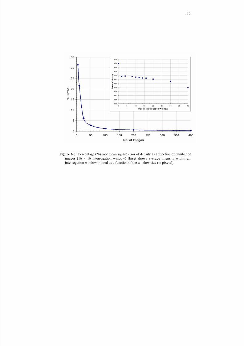
8/3/2019 Arindam Banerjee- Statistically Steady Measurements of Rayleigh-Taylor Mixing in a Gas Channel
http://slidepdf.com/reader/full/arindam-banerjee-statistically-steady-measurements-of-rayleigh-taylor-mixing 129/198
115
Figure 6.6 Percentage (%) root mean square error of density as a function of number of images (16 × 16 interrogation window) [Inset shows average intensity within aninterrogation window plotted as a function of the window size (in pixels)].
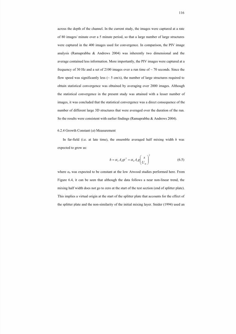
8/3/2019 Arindam Banerjee- Statistically Steady Measurements of Rayleigh-Taylor Mixing in a Gas Channel
http://slidepdf.com/reader/full/arindam-banerjee-statistically-steady-measurements-of-rayleigh-taylor-mixing 130/198
116
across the depth of the channel. In the current study, the images were captured at a rate
of 80 images/ minute over a 5 minute period, so that a large number of large structures
were captured in the 400 images used for convergence. In comparison, the PIV image
analysis (Ramaprabhu & Andrews 2004) was inherently two dimensional and the
average contained less information. More importantly, the PIV images were captured at a
frequency of 30 Hz and a set of 2100 images over a run time of ~ 70 seconds. Since the
flow speed was significantly less (~ 5 cm/s), the number of large structures required to
obtain statistical convergence was obtained by averaging over 2000 images. Although
the statistical convergence in the present study was attained with a lesser number of
images, it was concluded that the statistical convergence was a direct consequence of the
number of different large 3D structures that were averaged over the duration of the run.
So the results were consistent with earlier findings (Ramaprabhu & Andrews 2004).
6.2.4 Growth Constant (α ) Measurement
In far-field (i.e. at late time), the ensemble averaged half mixing width h was
expected to grow as:
2
2
⎟⎟ ⎠
⎞⎜⎜⎝
⎛ ==
m
t bt bU
x g A gt Ah α α (6.5)
where αBbB was expected to be constant at the low Atwood studies performed here. From
Figure 6.4, it can be seen that although the data follows a near non-linear trend, the
mixing half width does not go to zero at the start of the test section (end of splitter plate).
This implies a virtual origin at the start of the splitter plate that accounts for the effect of
the splitter plate and the non-similarity of the initial mixing layer. Snider (1994) used an
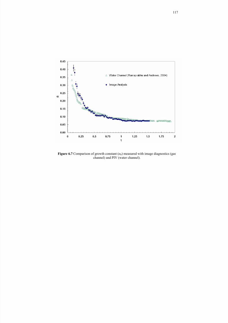
8/3/2019 Arindam Banerjee- Statistically Steady Measurements of Rayleigh-Taylor Mixing in a Gas Channel
http://slidepdf.com/reader/full/arindam-banerjee-statistically-steady-measurements-of-rayleigh-taylor-mixing 131/198
117
Figure 6.7 Comparison of growth constant (αBbB) measured with image diagnostics (gaschannel) and PIV (water channel).

8/3/2019 Arindam Banerjee- Statistically Steady Measurements of Rayleigh-Taylor Mixing in a Gas Channel
http://slidepdf.com/reader/full/arindam-banerjee-statistically-steady-measurements-of-rayleigh-taylor-mixing 132/198
118
absolute deviation algorithm which defines a virtual origin and fits a linear curve to the
mixing-half width to evaluate the growth constant. However, this technique was subject
to the accuracy of the fitting technique, but was accurate for getting a late-time saturated
estimate of αBbB. In the current study, a program was written that determined α based on a
“moving window” calculation. This technique used the half-mix width data as discussed
earlier in section C. A window with 10 pixels (2.5 cm) contained 10 mixing half widths
at each pixel location. The window was used to calculate a slope ( dxdh ) for the mixing
region by determining a 2P
ndP order polynomial best fit line through the data using a
method of least squares. The slope of the best fit line was used to calculate α within the
“window”. The window stepped along the downstream direction 1 pixel at a time and
calculated α at each location. The slope ( dxdh ) was used here as a measure of α to
better compare with the value of growth constant measured from hot-wire measurements
using the vertical velocity fluctuations v’ at the center-line (see Equation 6.5). Figure 6.7
shows a plot of α as a function of non-dimensional time τ [= 5.0)/( H g AU x t m ⋅ ], where
H was the height of the channel (1.2 m). Inspection of Figure 6.7 reveals that α
asymptotes to a value of 0.065- 0.07 suggesting that the flow reaches self-similarity in
this experiment ( ABtB # 0.035). Similar observations were recorded in earlier small Atwood
( ABt B~ 10P
-3P) studies (Ramaprabhu & Andrews 2004). The value of α measured at the
various Atwood number runs in the Gas Channel were compared with the LEM (Linear
Electric Motor) experiments of Dimonte (1996, 1999). As seen in Figure 6.7, our
measurements agree reasonably.

8/3/2019 Arindam Banerjee- Statistically Steady Measurements of Rayleigh-Taylor Mixing in a Gas Channel
http://slidepdf.com/reader/full/arindam-banerjee-statistically-steady-measurements-of-rayleigh-taylor-mixing 133/198
119
Figure 6.8 Comparison of growth constant (α) obtained by image analysis (at gaschannel) with LEM (Linear Electric Motor) experimental measurement of Dimonte &
Schneider (1996)

8/3/2019 Arindam Banerjee- Statistically Steady Measurements of Rayleigh-Taylor Mixing in a Gas Channel
http://slidepdf.com/reader/full/arindam-banerjee-statistically-steady-measurements-of-rayleigh-taylor-mixing 134/198
120
6.3 Hot-Wire Measurements
6.3.1 Measurements with Multi-position SN-Wire Technique
The density gradient needed to create a RT Instability was obtained by using a heavy
fluid (air) over a light one (air-helium mixture). This was different from the low Atwood
water channel experiments where the instability was created using cold water (heavy)
over hot water (light). However, the addition of helium to the mix caused a small
temperature gradient (~2º C) along the vertical ( y) direction (i.e. from the air to the
air/helium mixture). As already mentioned before, we took advantage of this small
temperature gradient and used a cold wire probe couple to a CCA unit to check for the
centerline of the mix. Initially, the cold-wire was placed close to the centerline of the
mixing layer by visual inspection and the data was logged. The centerline offset factor φ
was computed after the logging process as:
1
1−
⎥⎥⎦
⎤
⎢⎢⎣
⎡⎟⎟ ⎠
⎞⎜⎜⎝
⎛
−
−+=
topi
ibottom
top
bottom
top
p
bottom p
T T
T T
C
C
ρ
ρ φ (6.6)
where, bottom
pC and bottomT were the specific heat and temperature of the helium-air mixture
(flow at the bottom section of the channel); top
pC and topT were the specific heat and
temperature of air (flow at the top section of the channel) ; and iT was the temperature of
the mix. If ≠φ 0.5, the position of the cold-wire was readjusted and the data logging
process repeated. The cold-wire was adjusted until φ approaches a value of 0.5 with an
accuracy of 5%.

8/3/2019 Arindam Banerjee- Statistically Steady Measurements of Rayleigh-Taylor Mixing in a Gas Channel
http://slidepdf.com/reader/full/arindam-banerjee-statistically-steady-measurements-of-rayleigh-taylor-mixing 135/198
121
The hot-wire was placed at the center-line location at various downstream positions
from the splitter plate ( x = 1.0m, 1.75m and 1.95m). The centerline r.m.s. values of the
vertical, v’ , horizontal, u’ , and cross wise, w’ velocities were determined using the multi-
position single wire technique discussed in Section 4.3.1 at τ locations of 0.8126, 1.422
and 1.5845 (for x = 1.0m, 1.75m and 1.95m) from the splitter plate. The results were
tabulated in Table 6.2. Ramaprabhu and Andrews (2004) found that the vertical velocity
fluctuation (v’ ) at the centerline can be related to the centerline of the mix width by:
mt t U
x g At g A
dt
dhv α α 22 ===′ (6.7)
Thus, by using Equation 6.7 and the centerline value of v’ , we imply that the expansion
of the mix was driven by velocity fluctuations that occur across the whole mix and not
just the edge. This characterization was also supported by observations of the mixing
layer shown in Figure 6.1, where large-scale structures span the mix and dominate the
velocity fluctuations. Statistics measured in this region remain practically constant
across the mix. Thus it was convenient to determine the growth constant α by computing
the ratio, ( ) mt U x g Av 2′ . The measured ratio at the 3 downstream locations was
plotted as a function of non-dimensional time τ in Figure 6.9. It was seen that the results
agree with the value of α as found from image analysis by using a moving window
technique. Since the Atwood number of 0.035 used for the study was low, it was
expected that the dynamics of the R-T mix should be similar to that of the small Atwood

8/3/2019 Arindam Banerjee- Statistically Steady Measurements of Rayleigh-Taylor Mixing in a Gas Channel
http://slidepdf.com/reader/full/arindam-banerjee-statistically-steady-measurements-of-rayleigh-taylor-mixing 136/198
122
TABLE 6.2 Velocity fluctuations (m/s) measured at ABtBB B# 0.035 (U BmB= 0.6 m/s)
Distance from
splitter plate: x (m)1.0 1.75 1.95
u′ 0.0879 ± 0.002 0.0724 ± 0.001 0.0837 ± 0.0015
v′ 0.1051 ± 0.001 0.1286 ± 0.0012 0.1440 ± 0.0014
w′ 0.0729 ± 0.002 0.0709 ± 0.001 0.0753 ± 0.0015
mU u′ 0.1353 0.1114 0.1287
mU v′ 0.1617 0.1978 0.2216
uv ′′ 1.1951 ± 0.029 1.7747 ± 0.0369 1.7218 ± 0.0339
α 0.1004 ± 0.02 0.0702 ± 0.012 0.0706 ± 0.011
5.0
⎟ ⎠
⎞⎜⎝
⎛ =
H
g A
U
x t
m
τ 0.8126 1.4220 1.5845
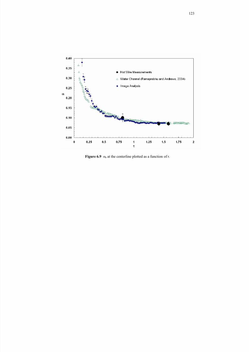
8/3/2019 Arindam Banerjee- Statistically Steady Measurements of Rayleigh-Taylor Mixing in a Gas Channel
http://slidepdf.com/reader/full/arindam-banerjee-statistically-steady-measurements-of-rayleigh-taylor-mixing 137/198
123
Figure 6.9 αB bB at the centerline plotted as a function of τ .

8/3/2019 Arindam Banerjee- Statistically Steady Measurements of Rayleigh-Taylor Mixing in a Gas Channel
http://slidepdf.com/reader/full/arindam-banerjee-statistically-steady-measurements-of-rayleigh-taylor-mixing 138/198
124
number runs in the water channel facility. Thus the growth constant obtained by PIV
measurements for a small Atwood run in the water channel was also plotted in Figure
6.9. All three sets of measurements of α agree reasonably well, and give a late time value
of 0.065 - 0.07. This consistency across measurement techniques (visualization, PIV and
hot-wire anemometry) and experiments (hot/cold water low Atwood facility, air/helium-
air high Atwood facility) demonstrated that the new facility provides consistent statistics
for the present experiment. The saturation of α at late time to a constant value of 0.07
was consistent with the measurements made at the small Atwood water channel facility
(Ramaprabhu & Andrews 2004). For low values of Atwood numbers used in the present
study, the value of αBbB is expected to be same for both bubbles and spikes (as the
structures were symmetric). However for high Atwood numbers (≥ 0.5), the value of α
would be different as the flow will be no longer symmetric but characterized by rising
bubbles and falling spikes (Dimonte 1999; Dimonte & Schneider 1996). So for higher
Atwood number (>0.1), Equation 6.7 would not give the same α as that based on mix
width measurements. However, it provides a well defined method for calculating an α
based on centerline velocity fluctuations that may be more convenient for validation
purposes (Banerjee & Andrews 2006).
6.3.2 Measurements with Multi-position Multi-Overheat Technique
The multi-position multi-overheat technique takes into account the density variations
in the flow and was used to measure velocity correlations ( vuvu ′′′′ ,, 22 ); velocity-
density correlations ( u′′ ρ , v′′ ρ ); as well as molecular mix parameters (θ , BB0B and BB2B).

8/3/2019 Arindam Banerjee- Statistically Steady Measurements of Rayleigh-Taylor Mixing in a Gas Channel
http://slidepdf.com/reader/full/arindam-banerjee-statistically-steady-measurements-of-rayleigh-taylor-mixing 139/198
125
Measurements were made at various downstream locations along the channel (see Table
6.1). Snider and Andrews (1994) has reported experiments which show that the side
walls do not affect the central region of the mix in the experimental set-up. The range of
density fluctuations and the extent of mixing in a Rayleigh-Taylor flow were
characterized by the following parameters:
2
0
11212
222
0
2
0
12
00 21
21
1
)1(
/)(
1
lim
1
1lim
1lim
B
B
f f f f B
dt T B
f f
dt T
dt T
f
T
T
T
hc
h
T
T
T
−=
−==
∆′=∆−=
−=
−
−=
−−
=
∫
∫ ∫
∞→
∞→∞→
θ
ρ ρ ρ ρ ρ
ρ ρ
ρ ρ
ρ ρ
ρ ρ
(6.8)
where, f BiB is the fraction by volume of the iP
thP fluid (with f B1B = f BheavyB, and f B2B = f Blight B). BB0B is the
intensity of turbulent density fluctuations and includes the effect of mixing due to
molecular diffusion. BB2B is the corresponding conditioned measure that would result if the
two fluids were immiscible and does not account for molecular mixing. Figure 6.10 plots
f B1B (defined as21
2
ρ ρ
ρ ρ
−
−, where ρ is the time-averaged density) across the mixing layer.
As might be expected at the present low Atwood number run the mix is symmetric about
the centerline. The total mix-width, 2h, was measured as the distance between the
locations where the average density was 5 % and 95 % of the heavier fluid (air).
The parameter θ (Danckwerts 1952) quantifies the degree of mixing with θ = 0
implies no mixing, and θ = 1 corresponding to completely molecularly mixed fluids. As

8/3/2019 Arindam Banerjee- Statistically Steady Measurements of Rayleigh-Taylor Mixing in a Gas Channel
http://slidepdf.com/reader/full/arindam-banerjee-statistically-steady-measurements-of-rayleigh-taylor-mixing 140/198
126
Figure 6.10 Density profiles measured with the multi-position multi-overheat hot-wiretechnique.

8/3/2019 Arindam Banerjee- Statistically Steady Measurements of Rayleigh-Taylor Mixing in a Gas Channel
http://slidepdf.com/reader/full/arindam-banerjee-statistically-steady-measurements-of-rayleigh-taylor-mixing 141/198
127
Figure 6.11 Molecular mix parameters across the mix at τ = 1.986 ( ABtB # 0.04, x=1.75 mfrom the splitter plate). The water channel measurements are by Wilson (2002).

8/3/2019 Arindam Banerjee- Statistically Steady Measurements of Rayleigh-Taylor Mixing in a Gas Channel
http://slidepdf.com/reader/full/arindam-banerjee-statistically-steady-measurements-of-rayleigh-taylor-mixing 142/198
128
explained in more detail later, BB2B may also be interpreted as an intermittency factor
based on the density of the fluids. The molecular mix θ affects the overall growth rate of
the mix in the following way. Consider the definitions of BB0B and BB2B as the non-
dimensional turbulent density fluctuations in the presence and absence of molecular
diffusion respectively. Then,
22
2212
22
00 / f f B , / B ρ ∆ ρ ρ ∆ ρ ′==′= (6.9)
where the 2
0 ρ ′ and 2
2 ρ ′ refer to the turbulent density fluctuations for the miscible and 2-
fluid cases respectively, and 21 ρ ρ ρ −=∆ . The growth rate of the mix may be rewritten
using the modified driving term 2
02 ρ ′ (Ramaprabhu & Andrews 2004)
)( gt 2h 21
2
0
2 ρ ρ ρ α +′= (6.10)
This was a more natural choice for molecularly mixed fluids, since the density difference
available to drive the flow 21 ρ ρ ρ ∆ −= was reduced in the presence of diffusion. For a
2-fluid case at the centerline where f B1B = f B2B = 0.5, then
4 / )( f f 2
21
2
21
2
2
2
0 ρ ρ ρ ∆ ρ ρ −==′=′ (6.11)
In this case, Equation 6.10 reduces to Equation 1.1.
For miscible fluids, we have
θ ρ
ρ −==
′
′1
2
0
22
2
0
B
B(6.12)
Equation 6.11 thus reduces to
2
t gt A~h α = (6.13)

8/3/2019 Arindam Banerjee- Statistically Steady Measurements of Rayleigh-Taylor Mixing in a Gas Channel
http://slidepdf.com/reader/full/arindam-banerjee-statistically-steady-measurements-of-rayleigh-taylor-mixing 143/198
129
Figure 6.12 Time evolution of scalar turbulence intensity and mix parameters measuredat the centerline (ABtB # 0.04). Water channel measurements are by Ramaprabhu and
Andrews (2004).

8/3/2019 Arindam Banerjee- Statistically Steady Measurements of Rayleigh-Taylor Mixing in a Gas Channel
http://slidepdf.com/reader/full/arindam-banerjee-statistically-steady-measurements-of-rayleigh-taylor-mixing 144/198
130
where θ α α −= 1~ . At the centerline of the mix, measurements of θ have been found to
vary from 0.7 to 0.8 (Ramaprabhu and Andrews 2004), and remain reasonably constant
across the mix (see Figure 6.11). Assuming an intermediate value of θ = 0.72, the
presence of molecular diffusion serves to reduce the growth rate of the mix by a factor of
0.53. The front tracking calculations of Glimm et al. (2001) suggest a 2-fluid value for α
of 0.07, giving a net growth constant == α α 53.0~ 0.037.
Figure 6.11 plots the molecular mix parameters across the mix. θ remains reasonably
constant across the mix and this is consistent with earlier results (Ramaprabhu &
Andrews 2004; Wilson 2002). It is seen that towards the edge of the mix, where the
probe sees more of one fluid than the other, the value of θ increases. The centerline time-
evolution of the mix-parameters defined above and determined from the hot-wire
measurements, were shown in Figure 6.12. Ramaprabhu and Andrews (2004) reported
measurements of θ close to the splitter plate (τ ~ 0.034). The mixing layer was diffuse
and, as a result, θ values were high in this region (and corresponding BB0B values were
low). As the mix develops farther downstream, the fluctuation levels increase with the
onset of the instability, resulting in a slight drop in the value of θ . The measurements
made at x = 50 cm (τ ∼ 0.567) correspond to this region. This effect was the result of
stretching of the initial diffuse layer, followed by rolling up into mushroom-shaped
structures. Eventually (τ ≥ 1.135), turbulent diffusion serves to smooth out some of
these fluctuations. As expected, the two-fluid parameter BB2B remains relatively constant at
a value of 0.25. This further confirms that these measurements were indeed at the

8/3/2019 Arindam Banerjee- Statistically Steady Measurements of Rayleigh-Taylor Mixing in a Gas Channel
http://slidepdf.com/reader/full/arindam-banerjee-statistically-steady-measurements-of-rayleigh-taylor-mixing 145/198
131
Figure 6.13 Comparison of measured α by different techniques (Hot-wire: MPMO:Multi-position Multi-overheat method; MP: Multi-position method) at ABtB # 0.04. Water
channel measurement was at ABtB # 7.5 x 10P
-4P.

8/3/2019 Arindam Banerjee- Statistically Steady Measurements of Rayleigh-Taylor Mixing in a Gas Channel
http://slidepdf.com/reader/full/arindam-banerjee-statistically-steady-measurements-of-rayleigh-taylor-mixing 146/198
132
centerline of the mix, since at the center f B1B = f B2B = 0.5 and BB2B = 0.25 according to
Equation 6.8. It was noteworthy that all the parameters change little in the developing
self-similar regime of the mix (τ > 1).
The centerline root mean square values of the vertical, v’ and horizontal, u’
velocities were determined using this technique at 7 downstream locations (for x =0.5m,
0.75 m, 1.0m, 1.25 m, 1.5m, 1.75m and 1.95m). The results were tabulated in Table 6.3.
By using Equation 6.7 and the centerline value of v’ , we imply that the expansion of the
mix was driven by velocity fluctuations that occur across the whole mix and not just the
edge. The v′ values grow linearly with time in the self-similar region. The growth
constant α was evaluated by computing the ratio: ( ) mt U x g Av 2′ . The measured ratio
at the 7 downstream locations was plotted as a function of non-dimensional time τ in
Figure 6.13. It is found that these measurements are consistent with the measurement
done with the multi-position single wire technique and also with the measurement of α
done with the visualization analysis.
Measurements were also made at different locations across the mix at a downstream
location of x = 1.75 m which corresponds to a τ of 1.986. The centerline of the mix was
found at the start of the run and the probe was moved in discrete steps (~ 9 cms) to
measure various parameters at 9 different locations across the mix. As can be seen with
Figure 6.10, the two end points are outside the mixing layer. Since our flow is a channel
type flow, we measure a small value of u’ at these locations. Figure 6.10 plots the
velocity correlations across the mix at x = 1.75 m (τ =1.986) for an experimental run at
Atwood # 0.04. Since there is no shear in this experiment, >< 2'v dominates over
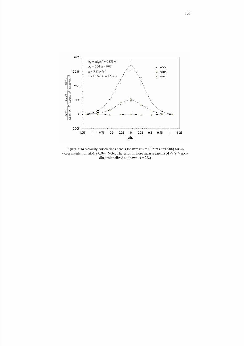
8/3/2019 Arindam Banerjee- Statistically Steady Measurements of Rayleigh-Taylor Mixing in a Gas Channel
http://slidepdf.com/reader/full/arindam-banerjee-statistically-steady-measurements-of-rayleigh-taylor-mixing 147/198
133
Figure 6.14 Velocity correlations across the mix at x = 1.75 m (τ =1.986) for anexperimental run at ABtB # 0.04. (Note: The error in these measurements of <u’v’> non-
dimensionalized as shown is ± 2%)

8/3/2019 Arindam Banerjee- Statistically Steady Measurements of Rayleigh-Taylor Mixing in a Gas Channel
http://slidepdf.com/reader/full/arindam-banerjee-statistically-steady-measurements-of-rayleigh-taylor-mixing 148/198
134
Figure 6.15 Ratio of u
v
′′
across the mix at x = 1.75 m (τ =1.986) for an experimental run
at ABtB # 0.04.

8/3/2019 Arindam Banerjee- Statistically Steady Measurements of Rayleigh-Taylor Mixing in a Gas Channel
http://slidepdf.com/reader/full/arindam-banerjee-statistically-steady-measurements-of-rayleigh-taylor-mixing 149/198
135
>′< 2u everywhere across the mix. The cross correlation term vu ′′ was also found to
be negligible since the mushroom-shaped structures have left-right symmetry about the
center, so thatleft right
vuvu '''' −= (Ramaprabhu & Andrews 2004). Furthermore, the ratio
u
v
′′
is almost constant across the mixing layer as seen in Figure 6.14. The primary
transport term in a R-T flow is the mass flux term < ρ′ v′ >, which can be computed from
the hot-wire data. The evolution of < ρ′ v′ > normalized by ∆ρ ( ABt B gx/U BmB)P
Pis shown in
Figure 6.15. It should be noted here that the term ABt B gx/U BmB is the “free-fall velocity”.P
PIt is
seen that the mass flux term reaches a constant value when the flow becomes self-
similar. Figure 6.16 shows the values of < ρ′ v′ > and < ρ′ u′ > across the mix at τ = 1.986.
It is seen that < ρ′ u′ > is negligible across the mixing layer, due once again to the left-
right symmetry of the mushroom-shaped structures, but < ρ′ v′ > has a peak that increases
in magnitude with distance downstream. The vertical mass flux is negative because a
packet of fluid that is lighter than its neighboring fluid particles ( 0<−≡′ ρ ρ ρ ) will
travel upwards with a velocity v′ (v′ > 0) and vice-versa, giving a negative correlation
between ρ′ and v′ .

8/3/2019 Arindam Banerjee- Statistically Steady Measurements of Rayleigh-Taylor Mixing in a Gas Channel
http://slidepdf.com/reader/full/arindam-banerjee-statistically-steady-measurements-of-rayleigh-taylor-mixing 150/198
136
Figure 6.16 Evolution of primary transport term for ABtB # 0.04.

8/3/2019 Arindam Banerjee- Statistically Steady Measurements of Rayleigh-Taylor Mixing in a Gas Channel
http://slidepdf.com/reader/full/arindam-banerjee-statistically-steady-measurements-of-rayleigh-taylor-mixing 151/198
137
Figure 6.17 Profile of < ρ′ v′ > and < ρ′ u′ > across the mix at τ = 1.986 for ABtB # 0.04(Note: The error in these measurements of < ρ’u’> non-dimensionalized as shown is
± 2.5 %)

8/3/2019 Arindam Banerjee- Statistically Steady Measurements of Rayleigh-Taylor Mixing in a Gas Channel
http://slidepdf.com/reader/full/arindam-banerjee-statistically-steady-measurements-of-rayleigh-taylor-mixing 152/198
138
6.4 Energy Budget
From our simultaneous measurements of velocity and density fields, the net kinetic
energy dissipation from the initial state of the flow is calculated based on previously
done similar calculations (Ramaprabhu & Andrews 2004; Youngs 1984). The initial
potential energy PE BiB, associated with the flow, is calculated assuming a step-function at z
= H /2 for the density profile at T = 0. Thus,
∫ ∫ ∫ +==
2
0 2 210
H H
H
H
stepi dz gz dz gz dz z PE ρ ρ ρ (6.14)
Also, at T = 0, KE BiB ~ 0, since there is negligible energy associated with velocity
fluctuations. Further downstream, the potential energy at τ = 1.96 is computed from the
measured density profile as
z z g dz z g PE i
n
i
i
H
f ∆≅= ∑∫ =0
0 ρ ρ (6.15)
The potential energy released to the flow by T = 1.96 is then given by PE Breleased B = PE B f B –
PE BiB. Some of this energy is converted into kinetic energy, which can be directly obtained
from our measured velocity profiles of u′ and v′ . Axisymmetric mushroom structures
mean we may take the turbulence as homogeneous with respect to the stream-wise
direction x and the span-wise direction z , and set <u′ P
2P> = <w′ P
2P>. Then,
∫ >′<+>′<= H
0
22
21
generated dz )vu2( KE ρ (6.16)
and the net kinetic energy dissipation is given by

8/3/2019 Arindam Banerjee- Statistically Steady Measurements of Rayleigh-Taylor Mixing in a Gas Channel
http://slidepdf.com/reader/full/arindam-banerjee-statistically-steady-measurements-of-rayleigh-taylor-mixing 153/198
139
D = PE Breleased B – KE B generated B. (6.17)
The net KE dissipation as a fraction of the potential energy released, D/PE Breleased B was
determined from our measurements to be 0.48 at τ ~ 1.96. Ramaprabhu and Andrews
(2004) obtained a value of 0.49 at τ ~ 1.21. Youngs (1984) reported a value of 0.52
obtained from 3D numerical simulations. The value obtained from 2D simulations was
significantly less ( D/PE Breleased B ~ 0.06) since dissipation is primarily a 3D mechanism. For
a self-similar mix, characterized by the length scale gt P2
P , it is expected that D/PE Breleased B
and KE B
generated B
/PE B
released B
become constant in the self-similar regime. Thus, we find good
agreement between the present experiments and related, but higher Atwood number, 3D
simulations.

8/3/2019 Arindam Banerjee- Statistically Steady Measurements of Rayleigh-Taylor Mixing in a Gas Channel
http://slidepdf.com/reader/full/arindam-banerjee-statistically-steady-measurements-of-rayleigh-taylor-mixing 154/198
140
7. CONCLUSIONS
A novel air-helium gas channel experiment was constructed to study the
development of high Atwood number Rayleigh-Taylor mixing. This dissertation reports
experimental runs for low Atwood numbers from 0.035 to 0.25. The experiment allows a
heavy fluid to be placed over a light fluid, and a long duration to study the mixing
process. Diagnostics used included constant temperature hot-wire anemometry and
digital image analysis. A multi-position single-wire technique was used to measure the
velocity fluctuations in three mutually perpendicular directions. However, this technique
did not take into consideration the effect of Helium on the measurements. So an
improvement over this technique, a multi-position multi-overheat technique was
developed to measure various velocity, density and velocity-density correlations in the
flow. Analysis of the measured data was used to explain the mixing as it develops to a
self-similar regime in this flow and also to provide for a value of the growth parameter
α. The significant conclusions of this work are summarized below:
• In this experiment, the Rayleigh-Taylor mix, after a stage of linear growth,
evolve through mode-interactions and successive wavelength saturation. The
fully-developed mix grows quadratically in time, with a self-similar structure.
• Characterization of the mix width development was done using centerline
vertical velocity fluctuations. The quadratic growth rate constant α was measured
at 0.065 using hot-wire anemometry. This was further verified with an image
analysis technique. The mixture fraction obtained from the visualization analysis

8/3/2019 Arindam Banerjee- Statistically Steady Measurements of Rayleigh-Taylor Mixing in a Gas Channel
http://slidepdf.com/reader/full/arindam-banerjee-statistically-steady-measurements-of-rayleigh-taylor-mixing 155/198
141
suggests that the air and helium-air mixture were linearly distributed across the
mixing layer. The value of α obtained by the visualization technique agreed well
with that obtained by the hot-wire method. To verify that errors were indeed
measurement errors and not as a result of lack of statistical convergence, a
detailed convergence test was performed. The study revealed that the statistical
convergence was a direct consequence of the number of different large 3D
structures that were averaged over the duration of the run. These measurements
good agreement with previous measurements from similar experiment (water
channel) using the mix width based on the 5% and 95% threshold for the volume
fractions. This verifies the fact that large-scale structures dominate the mixing
and contain most of the kinetic energy of the mix.
• The vertical velocity fluctuations dominating the horizontal (stream-wise and
transverse) components. The ratio of u
v′
′ is ~ 1.8, and appears to be constant
across the mix, as the mushroom-shaped structures are convected up and down
the mix without much change in shape. The internal structure of the self-similar
mix is thus anisotropic.
• From an energy budget analysis, it was shown that there is considerable kinetic
energy dissipation (~50% of the potential energy loss), which indicates the
presence of highly three-dimensional structures necessary for mixing to occur.
• The molecular mix fraction, a local mix parameter, was determined to be ~ 0.70
in the self-similar region. The value of the mix fraction was found to be almost
constant across the mix. Prandtl number and Schmidt number ~ 1 for the facility.

8/3/2019 Arindam Banerjee- Statistically Steady Measurements of Rayleigh-Taylor Mixing in a Gas Channel
http://slidepdf.com/reader/full/arindam-banerjee-statistically-steady-measurements-of-rayleigh-taylor-mixing 156/198
142
• A major improvement in the exit plenum design was the introduction of an “exit
splitter plate” in the exit section. A flap was also placed on the top half of the exit
section and was located about 24 inches from the test section. Since helium is
naturally buoyant, it was noticed that with an increase in the amount of helium in
the bottom half of the channel (with increase in Atwood number), the center-line
of the mix had a tendency to go up. To arrest this behavior and keep the center-
line more or less horizontal, an exit splitter plate was introduced and a flap was
placed on the top half of the channel. The opening of the flap was adjusted to
keep the center-line of the mix more or less horizontal in end of the test section.
• A new convective heat transfer correlation was formulated for variable-density
flows (binary gas mixture of air and helium) past a heated cylinder. The wire
diameter was sufficiently small for the effects of molecular nature of the fluid to
be experienced. Molecular effects take the form of changed boundary conditions
as compared with continuum flow – there was a jump in temperature between the
surface of the wire and the fluid adjacent to it. A continuum Nusselt number was
evaluated and the calibration data non-dimensionalized to obtain a working
correlation for variable density flows consisting of air-helium mixture. However,
because of the low velocities used in the experiment (U BmB < 2 m/s), the correlation
was limited to small Reynolds ( Re) numbers. Some scatter was observed in the
low Re regime which may be attributed to combined effects of forced and natural
convection.

8/3/2019 Arindam Banerjee- Statistically Steady Measurements of Rayleigh-Taylor Mixing in a Gas Channel
http://slidepdf.com/reader/full/arindam-banerjee-statistically-steady-measurements-of-rayleigh-taylor-mixing 157/198
143
• The multi-position multi-overheat method an “time-averaged” technique and was
initially thought to be robust enough to measure the various statistics for a wide
range of Atwood numbers for the flow. However, there are some major
limitations with this technique to be used in high Atwood number runs ( ABtB >
0.25). As described in section 4.3.2, the technique assumes a value of ρ d dE for
the entire density during the run. In practice, this is accurate if the response of E
vs. ρ is linear, which is the case for small density difference ( ABtB ~ 0.25). A value
of ρ d dE thus selected encompasses the entire range of densities accurately.
However, for large density differences ( ABtB > 0.25), the response becomes
significantly non-linear as can be seen in Figures 4.11 and 4.16. Using a linear
assumption (by calculating derivatives/sensitivities) would result in significant
errors in the measured quantities. Thus this method was not attempted for any
high Atwood measurements. The alternate technique to thus measure all density-
velocity correlations as well as evaluate spectral information is to pursue an
“instantaneous” technique by using a combination of a 3 wire probe (operated in
CTA mode) with a cold wire probe (operated in CCA mode) placed very close to
it. The cold-wire, which works as a resistance wire will measure instantaneous
density during a run. This information can then be used to correlate and solve for
the three-dimensional velocity fluctuations on an instantaneous basis. This is left
as a future work.

8/3/2019 Arindam Banerjee- Statistically Steady Measurements of Rayleigh-Taylor Mixing in a Gas Channel
http://slidepdf.com/reader/full/arindam-banerjee-statistically-steady-measurements-of-rayleigh-taylor-mixing 158/198
144
LITERATURE CITED
Acrivos A. 1966. On the combined effect of forced and free convection heat transfer inlaminar boundary layer flows. Chem. Eng. Sci. 21:343-52
Aihara Y, Kassoy DR, Libby PA. 1967. Heat transfer from cylinders at low Reynoldsnumbers. II. Experimental results and comparison with theory. Phys. Fluids 10:947-52
Allred JC, Blount GH. 1954. Experimental studies of Taylor instability, University of California report LA-I.600
Almquist P, Legath E. 1965. The hot-wire anemometer at low air velocities. DISA Info
2:3-4
Andrews GE, Bradley D, Hundy GF. 1972. Hot-wire anemometer calibration for measurements of small gas velocities. Int. J. Heat Mass Trans. 15:1765-86
Andrews MJ. 1986. Turbulent mixing by Rayleigh-Taylor instability. London: ImperialCollege
Andrews MJ, Spalding DB. 1990. A simple experiment to investigate two-dimensionalmixing by Rayleigh-Taylor instability. Phys. Fluids A 2:922-27
Anuchina NN, Kucherenko YA, Neuvazhaev VE, Ogibina VN, Shibarshov LI, et al.1978. Turbulent mixing at an accelerating interface between liquids of differentdensities. Translated from Izv. Akad Nauk. SSSR, Mekh. Zhidk. Gaza 6:157–60
Atzeni S, Meyer-ter-Vehn J. 2004. The physics of inertial fusion: beam plasmainteraction, hydrodynamics, hot dense matter. In International Monographs on Physics; ed. J Birman, SF Edwards, R Friend, M Rees, D Sherrington, GVeneziano, pp. 1-458. Oxford: Oxford University Press
Baid KM. 1967. Measurement of velocity in gas mixtures. MS thesis. Illinois Institute of Technology, Chicago
Banerjee A, Andrews MJ. 2006. Statistically steady measurements of Rayleigh-Taylor mixing in a gas channel. Phys. Fluids 18:1-13
Besnard D, Harlow FH, Rauenzahn R, Zemach C. 1990. Spectral transport model for turbulence. Los Alamos Report, LA-11821

8/3/2019 Arindam Banerjee- Statistically Steady Measurements of Rayleigh-Taylor Mixing in a Gas Channel
http://slidepdf.com/reader/full/arindam-banerjee-statistically-steady-measurements-of-rayleigh-taylor-mixing 159/198
145
Besnard D, Harlow FH, Rauenzahn R, Zemach C. 1992. Turbulence transport equationsfor variable density turbulence, and a relationship to two-fluid models. Los
Alamos Report, LA-11303
Betti R, Umansky M, Lobatchev V, Goncharov VN, McCrory RL. 2001. Hot-spotdynamics and deceleration-phase Rayleigh-Taylor instability of implodinginertial confinement fusion capsules. Phys. Plasmas 8:5257-67
Brouillette M. 2002. The Richtmyer-Meshkov instability. Annu. Rev. Fluid Mech. 34:445-68
Browand FK, Weidman PD. 1976. Large scales in the developing mixing layer. J.Fluid
Mech. 76:127-44
Brown GL, Roshko A. 1974. On density effects and large structures in turbulent mixing
layers. J. Fluid Mech. 64:775-816
Bruun HH. 1972. Hot-wire corrections in low and high turbulence intensity flows. J.
Phys. E: Sci. Instr. 5:812-18
Bruun HH. 1996. Hot-wire anemometry : principles and signal analysis. Oxford: OxfordUniversity Press
Bruun HH, Tropea C. 1985. The calibration of inclined hot-wire probes. J. Phys. E: Sci.
Inst. 18:405-13
Chandrasekhar S. 1961. Hydrodynamic and hydromagnetic stability. New York: Dover
Chassaing P, Harran G, Joly J. 1994. Density fluctuations in free turbulent binarymixing. J. Fluid Mech. 279:239-78
Chen TS, Mucoglu A. 1975. Buoyancy effects on forced convection along a verticalcylinder. J. Heat Trans. 97C:198-203
Clarke JS, Fisher HN, Mason RJ. 1973. Laser-driven implosion of spherical DT targetsto thermonuclear burn conditions. Phys. Rev. Lett. 30:89-92
Cole J, Roshko A. 1954. Heat transfer from wires at Reynolds numbers in the Oseenrange. Proc. Heat Trans. Fluid Mech. Inst., University of California, Berkeley.6:357-84
Cole RL, Tankin RS. 1973. Experimental study of Taylor instability. Physics of Fluids 16:1810-15

8/3/2019 Arindam Banerjee- Statistically Steady Measurements of Rayleigh-Taylor Mixing in a Gas Channel
http://slidepdf.com/reader/full/arindam-banerjee-statistically-steady-measurements-of-rayleigh-taylor-mixing 160/198
146
Collis DC, William MJ. 1959. Two-dimensional convection from heated wires at lowReynolds numbers. J. Fluid Mech. 6:357-84
Comte-Bellot G. 1976. Hot-wire anemometry. Ann. Rev. Fluid Mech. 8:209-31
Cook AW, Cabot W, Miller PL. 2004. The mixing transition in Rayleigh-Taylor instability. J. Fluid Mech. 511:333-62
Cook AW, Dimotakis PE. 2001. Transition stages of Rayleigh-Taylor instability between miscible fluids. J. Fluid Mech. 443:69-99
Corrisin S. 1949. Extended applications of the hot-wire anemometer, Rev. Sci. Instr.
18:469-71
Cui AQ, Street RL. 2004. Large-eddy simulation of coastal upwelling flow. Env. Fluid
Mech. 4:197-223
Dalziel SB, Linden PF, Youngs DL. 1999. Self-similarity and internal structure of turbulence induced by Rayleigh-Taylor instability. J. Fluid Mech. 399:1-48
Danckwerts PV. 1952. The definition and measurement of some characteristics of mixtures. Appl. Sci. Res 3:279-96
Deissler RG. 1964. Analysis of second-order slip flow and temperature jump boundaryconditions for rarefied gas. Int. J. Heat Mass Trans. 7:681-94
Dimonte G. 1999. Nonlinear evolution of the Rayleigh-Taylor and Richtmyer-Meshkovinstabilities. Phys. Plasmas 6:2009-15
Dimonte G, Schneider M. 1996. Turbulent Rayleigh-Taylor instability experiments withvariable acceleration. Phys. Rev. E 54:3740-43
Dimotakis PE. 2000. The mixing transition in turbulent flows. J.Fluid Mech. 409:69-98
DiPrima RC, Swinney HL. 1981. Hydrodynamic instabilities and the transition to
turbulence. Berlin: Springer.
Emmons HW, Chang CT, Watson BC. 1960. Taylor instability of finite surface waves. J. Fluid Mech. 7:177-93
Ezekwe CI, Pierce FJ, McAllister JE. 1978. Measured Reynolds stress tensors in a three-dimensional turbulent boundary layer. AIAA J. 16:645-46

8/3/2019 Arindam Banerjee- Statistically Steady Measurements of Rayleigh-Taylor Mixing in a Gas Channel
http://slidepdf.com/reader/full/arindam-banerjee-statistically-steady-measurements-of-rayleigh-taylor-mixing 161/198
147
Gebhart B, Pera L. 1970. Mixed convection from long horizontal cylinders. J.Fluid
Mech. 45:1-49
Goldstein RJ. 1996. Fluid mechanics measurements. New York:Hemisphere Publishing
Corporation
Gull SF. 1975. The X-ray, optical and radio properties of young supernova remnants. Royal Astronom. Soc. Monthly Notices. 171:263-78
Harion JL, Marinot MF, Camano B. 1996. An improved method for measuring velocityand concentration by thermo-anemometry in turbulent helium-air mixtures. Exp.
Fluids 22:174-82
Hinze JO. 1959. Turbulence: an introduction to its mechanism and theory: New York:McGrawHill
Jacobs JW, Caton I. 1988. Three-dimensional Rayleigh-Taylor instability. Part 2Experiment. J.Fluid Mech.187:353-71
Jacobs JW, Dalziel SB. 2005. Rayleigh-Taylor instability in complex stratification. J.
Fluid Mech. 542:251-79
Jitschin W, Weber U, Hartmann HK. 1995. Convenient primary gas flow meter. Vacuum 46:821-25
John JEA. 1984. Gas dynamics. New York: Prentice Hall
Jørgensen FE. 1996. The computer-controlled constant temperature anemometer: aspectsof set-up, probe calibration, data acquisition and data conversion. Meas. Sci.
Tech. 7:1378-87
Kaminsky M. 1965. Atomic and ionic impact phenomena on metal surfaces. Berlin:Springer
Kanevce G, Oka S. 1973. Correcting hot-wire readings for influence of fluid temperaturevariations. DISA Info. 15:21-4
Kassoy DR. 1967. Heat transfer from circular cylinders at low Reynolds numbers. I.Theory for variable property flow. Phys. Fluids 10:938-46
Kennard EH. 1938. Kinetic theory of gases. New York:McGraw Hill

8/3/2019 Arindam Banerjee- Statistically Steady Measurements of Rayleigh-Taylor Mixing in a Gas Channel
http://slidepdf.com/reader/full/arindam-banerjee-statistically-steady-measurements-of-rayleigh-taylor-mixing 162/198
148
King LV. 1914. On the convection of heat from small cylinders in a stream of fluid:determination of the convection constants of small platinum wires withapplications to hot-wire anemometry. Phil. Trans. Royal Soc. A214:373-432
Kline SJ, McClintock FA. 1953. Describing uncertainties in single-sample experiments.Mech. Eng. 75:3-8
Koop GK. 1976. Instability and turbulence in a stratified shear layer . PhD dissertation.University of Southern California, Los Angeles
Koppius AM, Trines GRM. 1976. The dependence of hot-wire calibration on gastemperature at low Reynolds numbers. Int. J. Heat Mass Trans. 19:967-74
Kovasznay LSG. 1950. The hot-wire anemometer in supersonic flow. J.Aero.Sci.
17:565-72
Kucherenko YA, Balabin SI, Ardashova RI, Kozelkov OE, Dulov AV, Romanov IA.2003. Experimental study of the influence of the stabilizing properties of transitional layers on the turbulent mixing evolution. Las. Part. Beams 21:369-73
Kucherenko YA, Balabin SI, Cherrey R, Haas JF. 1997. Experimental investigation intoinertial properties of Rayleigh-Taylor turbulence. Las. Part. Beams 15:25-31
LaRue JC, Deaton T, Gibson CH. 1975. Measurement of high-frequency turbulenttemperature. Rev. Sci. Instr. 46:757-64
Lee T, Budwig R. 1991. Two improved methods for low-speed hot-wire calibration.Meas. Sci. Tech. 1:643-46
Lewis DJ. 1950. The instability of liquid surfaces when accelerated in a direction perpendicular to their planes II. Proc. Royal Soc. London A 202:81-96
Linden PF, Redondo JM, Caulfield CP. 1992. Molecular mixing in Rayleigh-Taylor instability. In Advances in compressible turbulent mixing , ed. WP Dannevik, ACBuckingham, CE Leith, pp. 95-104
Lindl JD. 1998. Inertial confinement fusion: the quest for ignition and energy gain using
indirect drive. Berlin: Springer
Loehrke RI, Nagib HM. 1972. Experiments on management of free-stream turbulence. AGARD Report 598, Illinois Institute of Technology, Chicago
Manca O, Mastullo R, Mazzei P. 1988. Calibration of hot-wire probes at low velocitiesin air with variable temperature. Dantec Info. 6:6-8

8/3/2019 Arindam Banerjee- Statistically Steady Measurements of Rayleigh-Taylor Mixing in a Gas Channel
http://slidepdf.com/reader/full/arindam-banerjee-statistically-steady-measurements-of-rayleigh-taylor-mixing 163/198
149
Marmottant P, Villermaux E. 2004. On spray formation. J.Fluid Mech. 498:73-111
Mason EA, Saxena SC. 1958. Approximate formula for the thermal conductivity of gasmixtures. Phys. Fluids 1:361-69
McAdams WH. 1954. Heat transmission. New York: McGraw-Hill
McCarty R. 1973. Thermodynamic properties of helium 4 from 2 to 1500 K at pressuresup to 108 Pa. J. Phys. Chem. Ref. Data 2:923-1042
Meshkov EE. 1969. Instability of the interface of two gases accelerated by a shock wave.Sov. Fluid Dyn. 4:101-108
Molchanov OA. 2003. On the origin of low- and middler-latitude ionosphericturbulence. Phys.Chem.Earth 29:559-67
Mueschke N. 2004. An investigation on the influence of initial conditions on RT mixing .MS thesis. Texas A&M University, College Station
Mueschke N, Andrews MJ. 2005. Investigation of scalar measurement error in diffusionand mixing process. Exp. Fuids 40:165-76
Pierce FJ, Ezekwe CI. 1976. Comparison of Reynolds stress diagnostics by fixed androtating probes. AIAA J. 14:412-14
Pitts WM, McCaffrey BJ. 1986. Response behavior of hot-wires and films to flows of
different gases. J. Fluid Mech. 169:465-512
Popil R, Curzon FL. 1979. Production of reproducible Rayleigh-Taylor instabilities. Rev.
Sci. Instr. 50:1291-95
Preckshot GW, Gorman JW. 1958. Steady state longitudinal and radial temperaturedistribution in internally heated finite wires. Ind. Eng. Chem. Res. 50:837-48
Ramaprabhu P, Andrews MJ. 2003. Simultaneous measurement of velocity and densityin buoyancy driven mixing. Exp. Fluids 34:98-106
Ramaprabhu P, Andrews MJ. 2004. Experimental investigation of Rayleigh- Taylor mixing at small Atwood numbers. J. Fluid Mech. 502:233-71
Ratafia M. 1973. Experimental investigation of Rayleigh-Taylor instability. Phys. Fluids 16:1207-10
8/3/2019 Arindam Banerjee- Statistically Steady Measurements of Rayleigh-Taylor Mixing in a Gas Channel
http://slidepdf.com/reader/full/arindam-banerjee-statistically-steady-measurements-of-rayleigh-taylor-mixing 164/198
150
Rayleigh L. 1884. Investigation of the equilibrium of an incompressible heavy fluid of variable density. T Proc. London Math. Soc. T T14T: 170–77
Read KI. 1984. Experimental investigation of turbulent mixing by Rayleigh-Taylor
instability. Physica D 12:45-58
Richtmyer RD. 1960. Taylor Instability in shock acceleration of compressible fluids.Comm. Pure Appl. Math. 8:297-319
Roberts PD, Rose SJ, Thompson PC, Wright RJ. 1980. The stability of multiple shellICF targets. J. Phys D : Appl. Phys. 13:1957-69
Rose WC. 1973. The behavior of a compressible turbulent boundary layer in a shock-
wave-induced adverse pressure gradient . PhD dissertation. University of Washington, Seattle
Saddoughi SG, Veeravalli SV. 1996. Hot-wire anemometry behavior at very highfrequencies. Meas. Sci.Tech. 7:1297-300
Simpson RL, Wyatt WG. 1973. The behaviour of hot-film anemometers in gas mixtures. J. Phys. E: Sci. Instr.6:981-87
Smarr L, Wilson JR, Barton RT, Bowers RL. 1981. Rayleigh-Taylor overturn in super-nova core collapse. Astrophys.J. 246:515-25
Smith WJ. 2000. Modern optical engineering . New York: McGraw Hill
Snider DM. 1994. A study of buoyancy and shear mixing . PhD dissertation. Texas A&MUniversity, College Station
Snider DM, Andrews MJ. 1994. Rayleigh-Taylor and shear driven mixing with anunstable thermal stratification. Phys. Fluids 6:3324-34
Snider DM, Andrews MJ. 1995. An inexpensive method for quantitative data collectionfrom photographic prints. Meas. Sci. Tech. 6:502-6
Snider DM, Andrews MJ. 1996. The simulation of mixing layers driven by compound
buoyancy and shear. J.Fluids Eng. 118:370-76
Stanford RA, Libby PA. 1974. Further applications of hot-wire anemometry toturbulence measurements in helium-air mixtures. Phys. Fluids 17:1353-61
Steinkamp MJ, Clark T, Harlow FH. 1995. Stochastic interpenetration of fluids. Los
Alamos Report, LA-131016

8/3/2019 Arindam Banerjee- Statistically Steady Measurements of Rayleigh-Taylor Mixing in a Gas Channel
http://slidepdf.com/reader/full/arindam-banerjee-statistically-steady-measurements-of-rayleigh-taylor-mixing 165/198
151
Stillinger DC, Head MJ, Helland KN, Van Atta CW. 1983. A closed loop gravity drivenwater channel for density stratified flow. J. Fluid Mech. 131:73-89
Swaminathan MK, Rankin GW, Sridhar K. 1986. Evaluation of the basic systems of
equation for turbulence measurements using the Monte Carlo technique. J.Fluid Mech. 170:1-19
Tan-Atichat J, Nagib HM, Loehrke RI. 1982. Interaction of free-stream turbulence withscreens and grids: a balance between turbulence scales. J.Fluid Mech.114:501-28
Taylor GI. 1938 The spectrum of turbulence. Proc. Royal Soc. London Ser. A 164:476– 90
Taylor GI. 1950. The instability of liquid surfaces when accelerated in a direction perpendicular to their planes I. Proc.Royal Soc. London Ser.A 201:192-96
Tennekes H, Lumley J. 1994. A first course in turbulence. Cambridge: MIT Press
Thomas GO. 2003. The aerodynamic breakup of ligaments. Atom. Sprays13:117-29
Van der Hegge Zijnen BG. 1956. Modified correlation formulae for heat transfer bynatural and forced convection from horizontal cylinders. Appl. Sci.Res.6:129–40
Wasan DT, Baid KM. 1971. Measurement of velocity in gas mixtures: hot-wire and hot-film anemometry. AiChE J. 17:729-31
Way J, Libby PA. 1970. Hot-wire probes for measuring velocity and concentration inhelium and air mixture AIAA J. 8:976-78
Way J, Libby PA. 1971. Application of hot-wire anemometry and digital techniques tomeasurements in a turbulent helium jet . AIAA J. 9:1567-73
Wilke CR. 1950. A viscosity equation for gas mixtures. J. Chem. Phys. 18:517-19
Wilson PN. 2002. A study of buoyancy and shear driven turbulence within a closed
water channel . PhD dissertation. Texas A&M University, College Station
Wilson PN, Andrews MJ, Harlow F. 1999. Spectral non-equilibrium in a turbulentmixing layer. Phy. Fluids A 11:2425-33
Wilson PN, Andrews PN. 2002. Spectral measurements of Rayleigh-Taylor mixing atsmall Atwood number. Phys. Fluids A 14:938-45

8/3/2019 Arindam Banerjee- Statistically Steady Measurements of Rayleigh-Taylor Mixing in a Gas Channel
http://slidepdf.com/reader/full/arindam-banerjee-statistically-steady-measurements-of-rayleigh-taylor-mixing 166/198
152
Wu B, Molinas A. 2001. Choked flows through short contractions. J. Hydr. Eng. 127:657-62
Wu P, Libby PA. 1971. Heat transfer to cylinders in helium and helium–air mixtures.
Int. J. Heat .Mass Tran. 14:1071-77
Youngs DL. 1984. Numerical simulation of turbulent mixing by Rayleigh-Taylor instability. Physica D 12:32-44
Youngs DL. 1989. Modelling turbulent mixing by Rayleigh-Taylor instability. Physica
D 37:270-87

8/3/2019 Arindam Banerjee- Statistically Steady Measurements of Rayleigh-Taylor Mixing in a Gas Channel
http://slidepdf.com/reader/full/arindam-banerjee-statistically-steady-measurements-of-rayleigh-taylor-mixing 167/198
153
APPENDIX A
DESIGN BASIS
A.1 Design Basis of the Experiment
In the experiment of buoyant mixing with a stream-wise velocity, U BmB, the
requirement was that downstream behavior does not affect upstream mixing. Unlike
shear layers which grow linearly with distance, buoyancy mixing was approximately
parabolic and grows as axial distance squared. For an average fluid
quantity, ∫ =T
dt T
0
1ϕ ϕ , the steady two dimensional equation of motion can be illustrated
as:
⎟⎟ ⎠
⎞⎜⎜⎝
⎛
∂∂
+∂∂
Γ=∂∂
+∂∂
2
2
2
2
y x yv
xU m
ϕ ϕ ϕ ϕ (A.1)
where U BmB was the convective velocity, v was the cross stream mingling velocity and
Γ was the turbulent plus molecular diffusion constant. Since R-T experiments conducted
at our facility has shown that v ~0, the 2P
ndP term drops out. Defining x = U Bm Bt , Equation
A.1 simplifies into:
⎟⎟ ⎠
⎞⎜⎜⎝
⎛
∂∂
+∂∂
Γ=∂∂
2
2
2
2
2
1
yt U t m
ϕ ϕ ϕ (A.2)
This was approximately parabolic if:
2
2
2
2
2
1
yt U m ∂∂
<<∂∂ ϕ ϕ
(A.3)

8/3/2019 Arindam Banerjee- Statistically Steady Measurements of Rayleigh-Taylor Mixing in a Gas Channel
http://slidepdf.com/reader/full/arindam-banerjee-statistically-steady-measurements-of-rayleigh-taylor-mixing 168/198
154
Consider ϕ to be the volume fraction, f . If h was the half width of the mixing region,
then f for the upper half of the mixing layer may be approximated with a boundary layer
profile:
5.02
2
2
++−=h
y
h
y f (A.4)
At y =0 (interface), f = 0.5 and at y = h, f = 1.0. Assuming that the mixing layer grows
like a parabola, we substitute all relations into the PDE and get
2
222 4 ⎟⎟ ⎠
⎞⎜⎜⎝
⎛ =′>> dt
dht U m α (A.5)
We then apply Taylor’s Hypothesis (Taylor 1938) to convert the temporal derivative into
a spatial one. Noting that θ tanmm U dx
dhU
dt
dh=⎟⎟
⎠
⎞⎜⎜⎝
⎛ =⎟⎟
⎠
⎞⎜⎜⎝
⎛ , then 1)(tan 2 <<θ . A maximum
slope on the mixing width of 0.3 will give the approximate parabolic flow for the
buoyant mixing layer. The relation between U B
mB
, the mean convective velocity and AB
t B
, the
Atwood Number was thus:
3
12
<m
t
U
gAhα (A.6)
Thus for any given Atwood number, the minimum flow velocity which will satisfy the
parabolic approximation was tabulated in Table A.1.

8/3/2019 Arindam Banerjee- Statistically Steady Measurements of Rayleigh-Taylor Mixing in a Gas Channel
http://slidepdf.com/reader/full/arindam-banerjee-statistically-steady-measurements-of-rayleigh-taylor-mixing 169/198
155
TABLE A.1 Minimum flow velocity to satisfy parabolic approximation in gas channel
Atwood Number Minimum U BmB (m/s) U BmB for θ = 15º (m/s)
0.05 0.48 0.54
0.1 0.68 0.76
0.25 1.07 1.21
0.5 1.51 1.72
0.75 1.85 2.09

8/3/2019 Arindam Banerjee- Statistically Steady Measurements of Rayleigh-Taylor Mixing in a Gas Channel
http://slidepdf.com/reader/full/arindam-banerjee-statistically-steady-measurements-of-rayleigh-taylor-mixing 170/198
156
A.2 Gravity Current Effects In The Gas Channel
During initial high Atwood runs ( ABtB > 0.1), we witnessed problems in starting the
channel. This was attributed to a combination of the following factors:
(a) The bottom stream consisting of a lighter mass of air-helium mixture had to push
out a heavier mass of air sitting in the test section. To eliminate this, the channel
was initially filled with helium and a fan was used to circulate the air inside the
channel test section. This helped to reduce the density of the fluid inside the
channel. However, at high Atwood number runs ( ABtB ~ 0.25 and higher), it was
important that the channel be started at a velocity higher than the calculated U BmB.
Once the denser mass of air in the test section was pushed out, the dampers can
be adjusted to set the velocity back to the prescribed mean velocity.
(b) Since helium is naturally buoyant, it was noticed that with an increase in the
amount of helium in the bottom half of the channel (with increase in Atwood
number), the center-line of the mix had a tendency to go up. To arrest this
behavior and keep the center-line more or less horizontal, an exit splitter plate
was introduced and a flap was placed on the top half of the channel. The opening
of the flap was adjusted to maintain a flat center-line towards the end of the
channel.
(c) Gravity currents were found to induce a backflow in the Gas Channel. The exit
plenum was redesigned and rebuilt to eliminate the gravity current to flow back
into the test sections. A calculation in a square box provides a reasonable
estimate of the effects of the gravity current.

8/3/2019 Arindam Banerjee- Statistically Steady Measurements of Rayleigh-Taylor Mixing in a Gas Channel
http://slidepdf.com/reader/full/arindam-banerjee-statistically-steady-measurements-of-rayleigh-taylor-mixing 171/198
157
For Configuration 1, the initial Potential Energy, PE B1B, was given as:
( )21
3
0
2
0
11422
ρ ρ ρ ρ +=+= ∫ ∫ L
g zdz L
g zdz L
g PE
L L
(A.7)
For Configuration 2, the final Potential Energy, PEBf B , was given as:
( )21
3
2
2
2
0
12 38
ρ ρ ρ ρ +=+= ∫ ∫ L
g zdz gL zdz gL PE
L
L
L
(A.8)
The Potential Energy converted to Kinetic Energy was given by:
( ) ( ) )(8
384
21
3
21
3
21
3
21 ρ ρ ρ ρ ρ ρ −=+−+=−= L g L g L g PE PE KE (A.9a)
The KE in terms of the mean value of the velocity was:
22
212
)(2
1v
L KE ρ ρ += (A.9b)
Equating Equations B.3a and B.3b, we get :
22 21
212 gL A gL
vt
=⎟⎟ ⎠
⎞
⎜⎜⎝
⎛
+
−
= ρ ρ
ρ ρ
(A.10)
Using a similar analogy for the Gas Channel and using L = h = 60 cm, the vertical
velocity component of the gravity wave falling downwards in calculated for the various
run conditions in the channel (see Table A.2). This implies that for the low Atwood run
(i.e. ABtB # 0.05), the heavy air at the bottom should flow out at a velocity = 0.54 – 0.38 =
0.16 m/s. To facilitate this process, a flexible ducting connected to a bottom suction fan
was introduced into the test section to draw out the heavy mass of air. Once the heavy
mass was drawn out, the flexible ducting was withdrawn and the fan was switched off.

8/3/2019 Arindam Banerjee- Statistically Steady Measurements of Rayleigh-Taylor Mixing in a Gas Channel
http://slidepdf.com/reader/full/arindam-banerjee-statistically-steady-measurements-of-rayleigh-taylor-mixing 172/198
158
Figure A.1 Stable configurations ( ρB1B > ρB2B) in a square box (1m × 1m) used to calculateconversion from potential energy to kinetic energy.
ρB1 ρB2
ρB2
ρB1
Configuration 1 Configuration 2

8/3/2019 Arindam Banerjee- Statistically Steady Measurements of Rayleigh-Taylor Mixing in a Gas Channel
http://slidepdf.com/reader/full/arindam-banerjee-statistically-steady-measurements-of-rayleigh-taylor-mixing 173/198
159
TABLE A.2 Vertical velocity (v) of the gravity wave and mean flow velocity U BmB corresponding to different run conditions at a different Atwood numbers ( L = 0.6m)
Facility Atwood Number v (m/s) U Bm B(m/s) 21
22 vU mean ρ ρ −
0.05 0.383 0.54 0.142
0.10 0.542 0.76 0.231
0.25 0.858 1.21 0.175
0.50 1.213 1.72 -0.578
Gas
Channel
0.75 1.486 2.09 -1.941
Water
Channel7.5 x 10P
-4P 0.012 0.045 1.876
8/3/2019 Arindam Banerjee- Statistically Steady Measurements of Rayleigh-Taylor Mixing in a Gas Channel
http://slidepdf.com/reader/full/arindam-banerjee-statistically-steady-measurements-of-rayleigh-taylor-mixing 174/198
160
APPENDIX B
ERROR ANALYSIS
B.1 Error in Mass Flow Rate Measurement
For the experiment, the helium flow rates required for the entire range of Atwood
Numbers (0.035 – 0.75) varied from 0.0066 lbm/s to 0.282 lbm/s. To meet these flow
requirements, a wide range of orifice sizes (d ~ 0.033” – 0.25”) were calibrated. The
least count of the scale used for mass calibration was ± 0.01 lbs. Since a bottle full of
compressed helium (~ 2100 psig) was about 1.5 lbm heavier than an empty bottle (<
550psig), multiple bottles were used to ensure that the entire calibration run lasts at least
30 seconds. Hence the uncertainty in mass flow rate was evaluated as Hemw&
= 0.01/30 =
1.532 ×10P
-4P kg/s.
B.2 Error in Velocity Measurement
As described in Section 4, a proportioner meter (Aalborg, Inc) was used for
calibrating the hot-wire probes. The proportioner meter has two tubes which were
separately calibrated for air and helium flow-rates. Each tube has 150 printed volume
graduations along the length of the tube and can read upto a maximum volumetric flow-
rate of 1.1677×10P
-3P mP
3P/s for air and 1.1685 ×10 P
-3P mP
3P/s for helium. Based on our velocity
requirements, we used a ½” PVC pipe for calibration. The uncertainty of velocities was
obtained based on the diameter of the pipe used and a value of mU w = 0.0615 m/s was
taken for the ½” pipe.

8/3/2019 Arindam Banerjee- Statistically Steady Measurements of Rayleigh-Taylor Mixing in a Gas Channel
http://slidepdf.com/reader/full/arindam-banerjee-statistically-steady-measurements-of-rayleigh-taylor-mixing 175/198
161
B.3 Error in Atwood Number
A Kline-McClintock Uncertainty Analysis (1953) was performed on Equation B.1:
mixair
mixair t A
ρ ρ
ρ ρ
+
−= (B.1)
The uncertainty in the Atwood number was defined as:
( ) ( )
2
12
2
2
2
2
122
22
⎥⎥
⎦
⎤
⎢⎢
⎣
⎡
⎟⎟ ⎠
⎞⎜⎜⎝
⎛ ×
+
−+⎟
⎟ ⎠
⎞⎜⎜⎝
⎛ ×
+=
⎥⎥⎦
⎤
⎢⎢⎣
⎡⎟⎟ ⎠
⎞⎜⎜⎝
⎛ ×
∂
∂+⎟⎟
⎠
⎞⎜⎜⎝
⎛ ×
∂
∂=
amixair
amixair t
ww
w A
w A
w
mixair
air
mixair
mix
mix
t
air
t A
ρ ρ
ρ ρ
ρ ρ
ρ
ρ ρ
ρ
ρ ρ
(B.2)
where, ⎥⎦
⎤⎢⎣
⎡−+=
He
air
m
Heair mix
AU
m
ρ
ρ ρ ρ 1
&(B.3)
To find uncertainty of mix ρ , we perform Kline-McClintock Analysis on Equation B.3.
2
1
22
222
⎥⎥⎥⎥⎥
⎦
⎤
⎢⎢⎢⎢⎢
⎣
⎡
⎟⎟ ⎠
⎞⎜⎜⎝
⎛ ×
∂
∂+⎟⎟
⎠
⎞⎜⎜⎝
⎛ ×
∂
∂+
⎟⎟ ⎠
⎞⎜⎜⎝
⎛ ×
∂
∂+⎟⎟
⎠
⎞⎜⎜⎝
⎛ ×
∂
∂+⎟⎟
⎠
⎞⎜⎜⎝
⎛ ×
∂
∂
=
air c
m Heair
mix
ww A
wU
wm
w
w
He
mix A
c
mix
U
m
mixm
He
mix
air
mix
ρ
ρ
ρ
ρ
ρ ρ
ρ ρ
ρ
ρ &
&(B.4a)
Individual uncertainties for the various parameters in Equation B.4a were determined.
The temperature of the air and helium stream was measured using a E-type
thermocouple. Since the uncertainty of the temperature measurement was ± 0.01ºC, the
uncertainties of the densities of air and helium was determined from their respective
equations of state (see Appendix C) by considering a deviation of ± 0.01ºC from a

8/3/2019 Arindam Banerjee- Statistically Steady Measurements of Rayleigh-Taylor Mixing in a Gas Channel
http://slidepdf.com/reader/full/arindam-banerjee-statistically-steady-measurements-of-rayleigh-taylor-mixing 176/198
162
temperature of 20 ºC. The uncertainties were evaluated as:air
w ρ = 0.00366 kg/mP
3P and
Hew ρ = 0.004583 kg/ mP
3P. The uncertainty in velocity was evaluated as
mU w = 0.0154 m/s
while the uncertainty in the cross sectional area was estimated as Aw = 0.0001 mP
2P. The
uncertainty in the mass flow rate of helium was obtained as Hemw&
= 1.532 ×10P
-4P kg/s.
2
1
2
2
2
2
2
2
22
11
11
1
⎥⎥⎥⎥⎥
⎥⎥⎥⎥⎥
⎦
⎤
⎢⎢⎢⎢⎢
⎢⎢⎢⎢⎢
⎣
⎡
⎪⎭
⎪⎬⎫
⎪⎩
⎪⎨⎧
×⎟⎟ ⎠
⎞⎜⎜⎝
⎛ +
⎭
⎬⎫
⎩
⎨⎧
×⎟⎟
⎠
⎞⎜⎜
⎝
⎛ −
−+
⎭
⎬⎫
⎩
⎨⎧
×⎟⎟
⎠
⎞⎜⎜
⎝
⎛ −
−+
⎭⎬⎫
⎩⎨⎧
×⎟⎟ ⎠
⎞⎜⎜⎝
⎛ −+
⎭⎬⎫
⎩⎨⎧
×⎟⎟ ⎠
⎞⎜⎜⎝
⎛ −
=
He
m
Heair
mix
w AU
m
w
AU
mw
AU
m
w AU
w AU
m
w
He
air
m
He
A
He
air
m
He
U
He
air
m
He
m
He
air
m Hem
He
ρ
ρ
ρ
ρ
ρ
ρ
ρ
ρ
ρ
ρ
ρ
ρ
&
&&
&
&
(B.4b)
Assuming densities at a temperature of 20 ºC, i.e. air ρ = 1.21 kg/mP
3P and He ρ = 0.16585
kg/ mP
3P, the uncertainty in Atwood Number of the flow was evaluated and was tabulated
in Table B.1.

8/3/2019 Arindam Banerjee- Statistically Steady Measurements of Rayleigh-Taylor Mixing in a Gas Channel
http://slidepdf.com/reader/full/arindam-banerjee-statistically-steady-measurements-of-rayleigh-taylor-mixing 177/198
163
TABLE B.1 Uncertainty in Atwood number for various experimental run conditions
ABtB U BmB (m/s) Hem& (kg/s) ρ Bmix B(kg/mP
3P)
mixw ρ
t Aw
0.035 0.60 0.0030 1.1243 0.00929 ±0.0024
0.097 0.84 0.0106 0.9962 0.00662 ±0.0036
0.250 1.21 0.0345 0.7258 0.00509 ±0.0036
0.496 1.70 0.0805 0.4078 0.00435 ±0.0042
0.750 2.09 0.1287 0.1667 0.00409 ±0.0053

8/3/2019 Arindam Banerjee- Statistically Steady Measurements of Rayleigh-Taylor Mixing in a Gas Channel
http://slidepdf.com/reader/full/arindam-banerjee-statistically-steady-measurements-of-rayleigh-taylor-mixing 178/198
164
B.4 Error in Visualization
Snider and Andrews (1994) reported on the sources of fixed and random errors
associated with their dye experiment. Fixed errors such as variations in background
lighting were removed by employing the above correction during data analysis. Random
errors though often uncontrollable were small in a well designed experiment. The
volume fraction f Bv B, was a random variable determined at each pixel location of an image.
Since f BvB was a line average through the mixing layer, it was also an estimate of the mean
volume fraction, v f , which was obtained by averaging over all images. From the Central
Limit Theorem, the variance v f was given by
N
B )f ( 22
smokev == σ Var (B.5)
where BB2B was the normalized two-fluid density variance and N was the total number of
volume fraction measurements. The total number of volume fraction measurements was
the product of the number of images acquired in a run (400 in the 0.035 Atwood imaging
experiment) and the number of samples in the line average through the mix (361).
Through the center of the mix, the line average gave a very large sample because of the
relatively large net material flux through the centerline of the mix. The variance in the
measured v f close to the centerline was thus negligible (Wilson 2002). At the edge of
the mixing layer where v f was 0.05 or 0.95, the ratio decreases when total number of
image (~ 400), making the error about v f ± 0.025. This was also evident from the

8/3/2019 Arindam Banerjee- Statistically Steady Measurements of Rayleigh-Taylor Mixing in a Gas Channel
http://slidepdf.com/reader/full/arindam-banerjee-statistically-steady-measurements-of-rayleigh-taylor-mixing 179/198
165
wiggles observed in the fraction profiles at mixture fraction values of 0 and 1, shown in
Figure 6.3.
B.5 Error in Hot-Wire Measurements
Studies conducted by Pierce and Ezekwe (1976) and Ezekwe et al. (1978) reveal
that errors involved in use of a multi-position single wire probe were comparable to an
X- wire probe. There were two significant elements in the use of multi-position
measurements of turbulent fluctuations. Firstly, the method was based on sequential
measurement at different orientations and was sensitive to changes in flow condition.
Care was taken to ensure that the mean flow remained constant and the probe was placed
at the same location for each successive run. Secondly, since the mean flow field was
predominately one-dimensional ( 0== W V ), the technique of Bruun (1972) reduced to
three measurements instead of the six roll positions required to resolve a three
dimensional mean flow. This reduced the errors involved in the measurements as the
number of positions was cut in half. A Kline McClintock uncertainty analysis was
undertaken for the multi-position multi-overheat method. Swaminathan et al. (1986)
carried out an analysis for parallel probe-stem orientation in a flow field similar to the
one used here. They plotted the errors associated with the mean velocity as a function of
the turbulence intensity of the flow. Their study shows that if the turbulence intensity of
the flow varied between 10 - 12%, the maximum error associated with the SN-wire
measurements would be between 0.5 - 3.0%, which was consistent with our
observations.

8/3/2019 Arindam Banerjee- Statistically Steady Measurements of Rayleigh-Taylor Mixing in a Gas Channel
http://slidepdf.com/reader/full/arindam-banerjee-statistically-steady-measurements-of-rayleigh-taylor-mixing 180/198
166
APPENDIX C
PROPERTIES OF FLUIDS
C.1 Properties of Helium
(a) Density :Polynomial fit for Equation of State for Helium ( ρ in kg/mP
3P and T in °C) for
range of 0 – 50 °C at 1 atm (McCarty 1973) :
1426 10774853089.110381320.610804.1 −−− ×+×−×= T T He ρ (C.1)
(b) Viscosity: At 300 K, absolute viscosity (µ ) of helium was 20.1 × 10P
-6P kg/m s.
(c) Thermal conductivity: At 300 K, thermal conductivity (k ) of Helium was 0.149
W/mK.
(d) Specific Heat: At 300K, specific heat at constant pressure (C B pB) was 5200 J/kg K.
C.2 Properties of Air
(a) Density: Polynomial fit for Equation of State for Air for range of 0 – 50 °C at 1 atm
2895.10037.0102104102 243848 +−×−×+×−= −−− T T T T air ρ (C.2)
(b) Viscosity: At 300 K, absolute viscosity (µ ) of Air = 18.43 × 10P
-6P kg/m s.
(c) Thermal conductivity: At 300 K, thermal conductivity (k ) of Air = 0.0267 W/m K.
(d) Specific Heat: At 300K, specific heat at constant pressure (C B pB) was 1005 J/kg K.

8/3/2019 Arindam Banerjee- Statistically Steady Measurements of Rayleigh-Taylor Mixing in a Gas Channel
http://slidepdf.com/reader/full/arindam-banerjee-statistically-steady-measurements-of-rayleigh-taylor-mixing 181/198
167
APPENDIX D
CALIBRATION CURVE FITS & ANALYSIS SOFTWARE
D.1 Table-Curve 3D Fits for E= f(U, ρ )
Statistics for Wire # 1 @ Overheat Ratio 1.9
Rank 72 Eqn 1045 z=(a+bx+clny+d(lny)2+e(lny)3)/(1+fx+gx2+hlny+i(lny)2)
r2 Coef Det DF Adj r2 Fit Std Err F-value0.9977113513 0.9974212409 0.020107227 3923.4514176
Parm Value Std Error t-value 95.00% Confidence Limits P>|t|
a 1.597567133 0.011529454 138.5639871 1.574583587 1.62055068 0.00000b 0.146337686 0.056832895 2.574876487 0.03304338 0.259631991 0.01208c 1.336098575 0.254887787 5.241908967 0.827989058 1.844208092 0.00000d 0.283005712 0.136791988 2.06887638 0.010315869 0.555695556 0.04215e -0.34066712 0.040271311 -8.45930035 -0.42094651 -0.26038773 0.00000f -0.01302054 0.036464239 -0.35707696 -0.08571067 0.059669593 0.72208g 0.010817117 0.003417177 3.165512336 0.004005099 0.017629136 0.00227h 1.12825612 0.159137316 7.089827509 0.811021679 1.445490561 0.00000i 0.562145551 0.059854749 9.391828791 0.44282729 0.681463811 0.00000
X at Fn Zmin Y at Fn Zmin Fn Zmin0.3956258391 1.201 1.5609701989X at Fn Zmax Y at Fn Zmax Fn Zmax3.0192032989 0.16585 2.9855376207
ProcedureGaussElimr2 Coef Det DF Adj r2 Fit Std Err0.9977113513 0.9974212409 0.020107227Source Sum of Squares DF Mean Square F Statistic P>FRegr 12.690029 8 1.5862537 3923.45 0.00000Error 0.029109642 72 0.00040430058Total 12.719139 80
Description: WIre # 1 Overheat Ratio = 1.9
X Variable: U
Xmin: 0.3956258391 Xmax: 3.0192032989 Xrange: 2.6235774599Xmean: 1.4132804694 Xstd: 0.6879333639
Y Variable: densityYmin: 0.16585 Ymax: 1.201 Yrange: 1.03515Ymean: 0.6936487037 Ystd: 0.3380541175
Z Variable: EZmin: 1.5473983443 Zmax: 3.0141318645 Zrange: 1.4667335202Zmean: 2.1272326377 Zstd: 0.3987345464

8/3/2019 Arindam Banerjee- Statistically Steady Measurements of Rayleigh-Taylor Mixing in a Gas Channel
http://slidepdf.com/reader/full/arindam-banerjee-statistically-steady-measurements-of-rayleigh-taylor-mixing 182/198
168
Statistics for Wire # 1 @ Overheat Ratio 1.6
Rank 73 Eqn 1045 z=(a+bx+clny+d(lny)2+e(lny)3)/(1+fx+gx2+hlny+i(lny)2)
r2 Coef Det DF Adj r2 Fit Std Err F-value0.9974645004 0.9971385076 0.0181294158 3491.42131
Parm Value Std Error t-value 95.00% Confidence Limits P>|t|a 1.372360607 0.010487826 130.8527212 1.351448475 1.393272738 0.00000b 0.113413401 0.050924323 2.227096902 0.011873186 0.214953617 0.02911c 1.151771106 0.225227138 5.113820284 0.702680948 1.600861264 0.00000d 0.265377675 0.115064094 2.306346541 0.035946388 0.494808962 0.02401e -0.28411545 0.035787857 -7.93887861 -0.35547441 -0.21275649 0.00000f -0.0225251 0.0383284 -0.58768692 -0.09894976 0.053899559 0.55861g 0.011794476 0.003714531 3.17522649 0.004387912 0.019201039 0.00222h 1.116921313 0.163582617 6.827872858 0.790746838 1.443095788 0.00000i 0.55947936 0.061337143 9.12137955 0.437176571 0.68178215 0.00000
X at Fn Zmin Y at Fn Zmin Fn Zmin0.3956258391 1.201 1.344550273X at Fn Zmax Y at Fn Zmax Fn Zmax2.8842507801 0.16585 2.5642614803
ProcedureGaussElimr2 Coef Det DF Adj r2 Fit Std Err0.9974645004 0.9971385076 0.0181294158Source Sum of Squares DF Mean Square F Statistic P>FRegr 9.1803632 8 1.1475454 3491.42 0.00000
Error 0.023335976 71 0.00032867572Total 9.2036992 79
Description: Wire 1 Overheat Ratio = 1.6
X Variable: UXmin: 0.3956258391 Xmax: 2.8842507801 Xrange: 2.4886249411Xmean: 1.3958217673 Xstd: 0.67536498
Y Variable: densityYmin: 0.16585 Ymax: 1.201 Yrange: 1.03515Ymean: 0.6873068125 Ystd: 0.3353030748
Z Variable: EZmin: 1.3339 Zmax: 2.5920828496 Zrange: 1.2581828496Zmean: 1.8282989817 Zstd: 0.3413246571

8/3/2019 Arindam Banerjee- Statistically Steady Measurements of Rayleigh-Taylor Mixing in a Gas Channel
http://slidepdf.com/reader/full/arindam-banerjee-statistically-steady-measurements-of-rayleigh-taylor-mixing 183/198
169
Statistics for Wire # 2 @ Overheat Ratio 1.9
Rank 94 Eqn 1045 z=(a+bx+clny+d(lny)P
2P+e(lny)P
3P)/(1+fx+gxP
2P+hlny+i(lny)P
2P)
rP
2P Coef Det DF Adj rP
2P Fit Std Err F-value
0.9949220988 0.9942784212 0.0304227637 1763.3858
Parm Value Std Error t-value 95.00% Confidence Limits P>|t|a 1.601146136 0.015896172 100.7252667 1.569457697 1.632834576 0.00000b -0.03010811 0.079625043 -0.37812366 -0.18883773 0.128621509 0.70645c 0.709512864 0.390172234 1.818460673 -0.06828127 1.487306998 0.07315d 0.630059365 0.183635538 3.43103176 0.263988609 0.99613012 0.00100e -0.32691708 0.063336565 -5.16158521 -0.45317621 -0.20065794 0.00000f -0.11250296 0.050668786 -2.2203603 -0.21350934 -0.01149658 0.02954g 0.013982988 0.004823267 2.899070111 0.004367982 0.023597995 0.00496h 0.732352438 0.236470754 3.097010633 0.260956606 1.20374827 0.00279i 0.588258239 0.096790393 6.077651082 0.395310116 0.781206362 0.00000
X at Fn Zmin Y at Fn Zmin Fn Zmin0.2444859143 1.201 1.546191022X at Fn Zmax Y at Fn Zmax Fn Zmax3.0192032989 0.16585 3.0383835721
ProcedureGaussElimrP
2P Coef Det DF Adj rP
2P Fit Std Err
0.9949220988 0.9942784212 0.0304227637Source Sum of Squares DF Mean Square F Statistic P>FRegr 13.056737 8 1.6320921 1763.39 0.00000Error 0.066639208 72 0.00092554455
Total 13.123376 80
Description: Wire 2 OR 1.9
X Variable: UXmin: 0.2444859143 Xmax: 3.0192032989 Xrange: 2.7747173846Xmean: 1.4099503227 Xstd: 0.6925415815
Y Variable: densityYmin: 0.16585 Ymax: 1.201 Yrange: 1.03515Ymean: 0.6936487037 Ystd: 0.3380541175
Z Variable: EZmin: 1.535509596 Zmax: 3.0173099995 Zrange: 1.4818004035Zmean: 2.1310283157 Zstd: 0.4050212364

8/3/2019 Arindam Banerjee- Statistically Steady Measurements of Rayleigh-Taylor Mixing in a Gas Channel
http://slidepdf.com/reader/full/arindam-banerjee-statistically-steady-measurements-of-rayleigh-taylor-mixing 184/198
170
Statistics for Wire # 2 @ Overheat Ratio 1.6
Rank 241 Eqn 1045 z=(a+bx+clny+d(lny)P
2P+e(lny)P
3P)/(1+fx+gxP
2P+hlny+i(lny)P
2P)
rP
2P Coef Det DF Adj rP
2P Fit Std Err F-value
0.9900189948 0.9887537969 0.0362575999 892.7127834
Parm Value Std Error t-value 95.00% Confidence Limits P>|t|a 1.351239598 0.019098402 70.75144762 1.313167629 1.389311567 0.00000b -0.16850111 0.090209132 -1.86789414 -0.34832973 0.011327509 0.06585c 0.166329933 0.436832679 0.380763486 -0.7044801 1.037139963 0.70450d 0.827636942 0.195697694 4.229160426 0.437520719 1.217753164 0.00007e -0.25085822 0.071317698 -3.51747502 -0.39302746 -0.10868899 0.00076f -0.22654812 0.067813342 -3.34076029 -0.36173154 -0.09136469 0.00133g 0.022792657 0.006741552 3.380921159 0.009353618 0.036231696 0.00117h 0.371168077 0.308308796 1.203884162 -0.24343428 0.98577043 0.23258i 0.602162332 0.128871363 4.672584478 0.345261964 0.8590627 0.00001
X at Fn Zmin Y at Fn Zmin Fn Zmin0.2444859143 1.201 1.3215901449X at Fn Zmax Y at Fn Zmax Fn Zmax3.0192032989 0.16585 2.5935416098
ProcedureGaussElimrP
2P Coef Det DF Adj rP
2P Fit Std Err
0.9900189948 0.9887537969 0.0362575999Source Sum of Squares DF Mean Square F Statistic P>FRegr 9.3885786 8 1.1735723 892.713 0.00000Error 0.094652176 72 0.0013146135
Total 9.4832307 80
Description: Wire 2 OR 1.6
X Variable: UXmin: 0.2444859143 Xmax: 3.0192032989 Xrange: 2.7747173846Xmean: 1.4083486408 Xstd: 0.6920767533
Y Variable: densityYmin: 0.16585 Ymax: 1.201 Yrange: 1.03515Ymean: 0.6936487037 Ystd: 0.3380541175
Z Variable: EZmin: 1.3107898392 Zmax: 2.5703616892 Zrange: 1.25957185Zmean: 1.8144332379 Zstd: 0.3442969419

8/3/2019 Arindam Banerjee- Statistically Steady Measurements of Rayleigh-Taylor Mixing in a Gas Channel
http://slidepdf.com/reader/full/arindam-banerjee-statistically-steady-measurements-of-rayleigh-taylor-mixing 185/198
171
Statistics for Wire # 3 @ Overheat Ratio 1.9
Rank 57 Eqn 1045 z=(a+bx+clny+d(lny)P
2P+e(lny)P
3P)/(1+fx+gxP
2P+hlny+i(lny)P
2P)
rP
2P Coef Det DF Adj rP
2P Fit Std Err F-value
0.9990933242 0.9989783934 0.0133819831 9917.3702747
Parm Value Std Error t-value 95.00% Confidence Limits P>|t|a 1.665437866 0.007233693 230.2334069 1.651017762 1.67985797 0.00000b -0.00973969 0.044769157 -0.21755353 -0.09898537 0.079505995 0.82839c 0.607496352 0.188352893 3.225309381 0.232021723 0.982970982 0.00189d 0.608484511 0.101319832 6.005581495 0.406507116 0.810461905 0.00000e -0.31246583 0.027109153 -11.5262115 -0.36650694 -0.25842473 0.00000f -0.11734193 0.026803272 -4.37789564 -0.17077328 -0.06391058 0.00004g 0.017656372 0.002243834 7.868840976 0.013183371 0.022129374 0.00000h 0.65093585 0.112824733 5.76944286 0.426023855 0.875847845 0.00000i 0.5325526 0.037851832 14.06940105 0.457096352 0.608008847 0.00000
X at Fn Zmin Y at Fn Zmin Fn Zmin0.2444859143 1.201 1.6159437137X at Fn Zmax Y at Fn Zmax Fn Zmax2.9517522199 0.16585 3.1845791151
ProcedureGaussElimrP
2P Coef Det DF Adj rP
2P Fit Std Err
0.9990933242 0.9989783934 0.0133819831Source Sum of Squares DF Mean Square F Statistic P>FRegr 14.207821 8 1.7759776 9917.37 0.00000Error 0.012893578 72 0.00017907747
Total 14.220714 80
Description: Wire 3 OR 1.9
X Variable: UXmin: 0.2444859143 Xmax: 2.9517522199 Xrange: 2.7072663055Xmean: 1.4091175933 Xstd: 0.6906202751
Y Variable: densityYmin: 0.16585 Ymax: 1.201 Yrange: 1.03515Ymean: 0.6936487037 Ystd: 0.3380541175
Z Variable: EZmin: 1.5829157049 Zmax: 3.1817187346 Zrange: 1.5988030297Zmean: 2.2430352037 Zstd: 0.4216146701

8/3/2019 Arindam Banerjee- Statistically Steady Measurements of Rayleigh-Taylor Mixing in a Gas Channel
http://slidepdf.com/reader/full/arindam-banerjee-statistically-steady-measurements-of-rayleigh-taylor-mixing 186/198
172
Statistics for Wire # 3 @ Overheat Ratio 1.6
Rank 51 Eqn 1045 z=(a+bx+clny+d(lny)P
2P+e(lny)P
3P)/(1+fx+gxP
2P+hlny+i(lny)P
2P)
rP
2P Coef Det DF Adj rP
2P Fit Std Err F-value
0.9992785047 0.9991870476 0.0101028739 12465.094188
Parm Value Std Error t-value 95.00% Confidence Limits P>|t|a 1.441007623 0.00543125 265.3178563 1.430180624 1.451834622 0.00000b 0.040619202 0.032194233 1.261691866 -0.02355883 0.104797234 0.21113c 0.720049688 0.13680366 5.263380298 0.447336576 0.9927628 0.00000d 0.360066215 0.066352876 5.426535162 0.227794174 0.492338256 0.00000e -0.27152962 0.019923557 -13.6285714 -0.31124651 -0.23181274 0.00000f -0.08085121 0.022436109 -3.60361991 -0.12557678 -0.03612564 0.00057g 0.015140754 0.00192054 7.883593717 0.011312228 0.018969279 0.00000h 0.790022957 0.094462147 8.363381354 0.601716109 0.978329806 0.00000i 0.503828797 0.03267649 15.41869369 0.438689404 0.56896819 0.00000
X at Fn Zmin Y at Fn Zmin Fn Zmin0.2444859143 1.201 1.3942238457X at Fn Zmax Y at Fn Zmax Fn Zmax3.0192032989 0.16585 2.7315137502
ProcedureGaussElimrP
2P Coef Det DF Adj rP
2P Fit Std Err
0.9992785047 0.9991870476 0.0101028739Source Sum of Squares DF Mean Square F Statistic P>FRegr 10.178304 8 1.272288 12465.1
0.00000
Error 0.0073489003 72 0.00010206806Total 10.185653 80
Description: Wire 3 OR 1.6
X Variable: UXmin: 0.2444859143 Xmax: 3.0192032989 Xrange: 2.7747173846Xmean: 1.4083486408 Xstd: 0.6920767533
Y Variable: densityYmin: 0.16585 Ymax: 1.201 Yrange: 1.03515Ymean: 0.6936487037 Ystd: 0.3380541175
Z Variable: EZmin: 1.3858086175 Zmax: 2.7318 Zrange: 1.3459913825Zmean: 1.9250929243 Zstd: 0.3568202064

8/3/2019 Arindam Banerjee- Statistically Steady Measurements of Rayleigh-Taylor Mixing in a Gas Channel
http://slidepdf.com/reader/full/arindam-banerjee-statistically-steady-measurements-of-rayleigh-taylor-mixing 187/198
173
D.2 Table-Curve 3D Fits for E= f(U, θ )
Statistics for Wire # 1 @ Overheat Ratio 1.9
Rank 22 Eqn 1303 z=(a+clnx+ey+g(lnx)P
2P+iyP
2P+kylnx)/(1+blnx+dy+f(lnx)P
2P+hyP
2P+jylnx)
rP
2PCoef Det DF Adj rP
2P Fit Std Err F-value
0.9995147458 0.9993529944 0.0019583292 7003.2367144
Parm Value Std Error t-value 95.00% Confidence Limits P>|t|a 1.475824144 0.007869679 187.5329617 1.459831032 1.491817255 0.00000b -0.28427433 0.06048153 -4.70018423 -0.40718759 -0.16136108 0.00004c -0.37247819 0.092262774 -4.03714491 -0.5599787 -0.18497767 0.00029d -0.12640027 0.090178225 -1.40167177 -0.30966447 0.05686393 0.17008e -0.00053468 0.157045607 -0.00340465 -0.31968976 0.318620387 0.99730f 0.039219844 0.016999352 2.307137555 0.004673004 0.073766685 0.02727
g 0.056463086 0.02521095 2.239625427 0.00522827 0.107697901 0.03176h 0.036278739 0.028317399 1.281146556 -0.02126914 0.093826618 0.20881i -0.00605342 0.049086069 -0.12332261 -0.10580832 0.093701472 0.90258
j 0.004898091 0.012028149 0.407219057 -0.01954605 0.02934223 0.68640k 0.006813322 0.018458106 0.369123588 -0.03069806 0.044324707 0.71432
X at Fn Zmin Y at Fn Zmin Fn Zmin0.3956258391 0.5235987756 1.5052091602X at Fn Zmax Y at Fn Zmax Fn Zmax3.0192032989 1.574231823 1.7832775762
ProcedureGaussElimrP
2P Coef Det DF Adj rP
2P Fit Std Err
0.9995147458 0.9993529944 0.0019583292Source Sum of Squares DF Mean Square F Statistic P>FRegr 0.26857786 10 0.026857786 7003.24
0.00000Error 0.00013039181 34 3.8350533e-06Total 0.26870825 44
Description: OR=1.9
X Variable: UXmin: 0.3956258391 Xmax: 3.0192032989 Xrange: 2.6235774599Xmean: 1.6816058445 Xstd: 0.9437646045
Y Variable: angleYmin: 0.5235987756 Ymax: 2.617993878 Yrange: 2.0943951024Ymean: 1.5707963268 Ystd: 0.6836013564
Z Variable: EZmin: 1.505531525 Zmax: 1.7837676317 Zrange: 0.2782361067Zmean: 1.6470391601 Zstd: 0.0781473335

8/3/2019 Arindam Banerjee- Statistically Steady Measurements of Rayleigh-Taylor Mixing in a Gas Channel
http://slidepdf.com/reader/full/arindam-banerjee-statistically-steady-measurements-of-rayleigh-taylor-mixing 188/198
174
Statistics for Wire # 1 @ Overheat Ratio 1.6
Rank 13 Eqn 1303 z=(a+clnx+ey+g(lnx)P
2P+iyP
2P+kylnx)/(1+blnx+dy+f(lnx)P
2P+hyP
2P+jylnx)
rP
2P Coef Det DF Adj rP
2P Fit Std Err F-value
0.9996491116 0.9995321488 0.0014702031 9686.2915203
Parm Value Std Error t-value 95.00% Confidence Limits P>|t|a 1.25511155 0.006280124 199.8545671 1.242348801 1.267874298 0.00000b -0.33243229 0.050064093 -6.64013399 -0.43417477 -0.23068981 0.00000c -0.37790052 0.06537744 -5.78028942 -0.51076347 -0.24503758 0.00000d 0.015406377 0.079792468 0.193080589 -0.14675143 0.177564182 0.84804e 0.219580206 0.12009047 1.82845655 -0.02447299 0.463633404 0.07627f 0.037236431 0.013819685 2.694448705 0.009151453 0.065321409 0.01087g 0.041637642 0.017692587 2.353394809 0.00568198 0.077593305 0.02453h -0.00819299 0.024889249 -0.32917807 -0.05877403 0.042388045 0.74404i -0.07434363 0.037336234 -1.99119252 -0.15021998 0.001532727 0.05454
j 0.00385509 0.009843144 0.391652329 -0.01614858 0.023858765 0.69776
k 0.004537461 0.012987497 0.349371483 -0.02185631 0.03093123 0.72897
X at Fn Zmin Y at Fn Zmin Fn Zmin0.3956258391 0.5235987756 1.2897549055X at Fn Zmax Y at Fn Zmax Fn Zmax3.0192032989 1.5737276419 1.5355980971
ProcedureGaussElimrP
2P Coef Det DF Adj rP
2P Fit Std Err
0.9996491116 0.9995321488 0.0014702031Source Sum of Squares DF Mean Square F Statistic P>F
Regr 0.20936891 10 0.020936891 9686.290.00000
Error 7.3490901e-05 34 2.1614971e-06Total 0.2094424 44
Description: OR=1.6
X Variable: OR=1.6Xmin: 0.3956258391 Xmax: 3.0192032989 Xrange: 2.6235774599Xmean: 1.678577174 Xstd: 0.9417026013
Y Variable: angleYmin: 0.5235987756 Ymax: 2.617993878 Yrange: 2.0943951024
Ymean: 1.5707963268 Ystd: 0.6836013564
Z Variable: EZmin: 1.2891456302 Zmax: 1.5345410943 Zrange: 0.2453954641Zmean: 1.4173058002 Zstd: 0.0689931484

8/3/2019 Arindam Banerjee- Statistically Steady Measurements of Rayleigh-Taylor Mixing in a Gas Channel
http://slidepdf.com/reader/full/arindam-banerjee-statistically-steady-measurements-of-rayleigh-taylor-mixing 189/198
175
Statistics for Wire # 2 @ Overheat Ratio 1.9
Rank 20 Eqn 1303 z=(a+clnx+ey+g(lnx)P
2P+iyP
2P+kylnx)/(1+blnx+dy+f(lnx)P
2P+hyP
2P+jylnx)
rP
2P Coef Det DF Adj rP
2P Fit Std Err F-value
0.9993415652 0.9991220869 0.0024503355 5160.3609714
Parm Value Std Error t-value 95.00% Confidence Limits P>|t|a 1.528483495 0.010434573 146.4826052 1.507277891 1.5496891 0.00000b -0.14127707 0.074897179 -1.88628019 -0.29348645 0.010932316 0.06782c -0.14263224 0.116625578 -1.22299282 -0.37964393 0.094379445 0.22974d -0.0859427 0.124695202 -0.68922222 -0.33935384 0.167468435 0.49536e 0.052526736 0.222556423 0.236015368 -0.39976233 0.504815804 0.81484f -0.06697387 0.01648477 -4.06277278 -0.10047496 -0.03347279 0.00027g -0.11115456 0.026369696 -4.21523868 -0.16474423 -0.05756489 0.00017h 0.020536696 0.03918836 0.524050928 -0.05910363 0.100177026 0.60364i -0.02778837 0.069735283 -0.3984837 -0.16950752 0.113930773 0.69277
j 0.005595253 0.012202244 0.458543004 -0.01920269 0.030393196 0.64948
k 0.007108192 0.019270013 0.368873251 -0.03205319 0.046269571 0.71451
X at Fn Zmin Y at Fn Zmin Fn Zmin0.3956258391 0.5235987756 1.5335538162X at Fn Zmax Y at Fn Zmax Fn Zmax3.0192032989 1.578799829 1.83482394
ProcedureGaussElimrP
2PCoef Det DF Adj rP
2P Fit Std Err
0.9993415652 0.9991220869 0.0024503355Source Sum of Squares DF Mean Square F Statistic P>F
Regr 0.30983552 10 0.030983552 5160.360.00000
Error 0.0002041409 34 6.0041442e-06Total 0.31003966 44
Description: OR=1.9
X Variable: UXmin: 0.3956258391 Xmax: 3.0192032989 Xrange: 2.6235774599Xmean: 1.6816058445 Xstd: 0.9437646045
Y Variable: angleYmin: 0.5235987756 Ymax: 2.617993878 Yrange: 2.0943951024
Ymean: 1.5707963268 Ystd: 0.6836013564
Z Variable: EZmin: 1.5301435215 Zmax: 1.8347450719 Zrange: 0.3046015505Zmean: 1.6949579935 Zstd: 0.0839425746

8/3/2019 Arindam Banerjee- Statistically Steady Measurements of Rayleigh-Taylor Mixing in a Gas Channel
http://slidepdf.com/reader/full/arindam-banerjee-statistically-steady-measurements-of-rayleigh-taylor-mixing 190/198
176
Statistics for Wire # 2 @ Overheat Ratio 1.6
Rank 49 Eqn 1303 z=(a+clnx+ey+g(lnx)P
2P+iyP
2P+kylnx)/(1+blnx+dy+f(lnx)P
2P+hyP
2P+jylnx)
rP
2P Coef Det DF Adj rP
2P Fit Std Err F-value
0.9989850208 0.9986466944 0.0026439595 3346.4223228
Parm Value Std Error t-value 95.00% Confidence Limits P>|t|a 1.330108429 0.009212763 144.3767136 1.311385842 1.348831016 0.00000b -0.05990494 0.095797984 -0.62532572 -0.25458987 0.134779984 0.53593c -0.01906461 0.128814992 -0.14799994 -0.28084817 0.242718948 0.88322d -0.38832172 0.130345822 -2.97916506 -0.6532163 -0.12342714 0.00530e -0.41753146 0.198603831 -2.10233334 -0.821143 -0.01391991 0.04301f -0.02245782 0.023846549 -0.94176388 -0.07091984 0.026004199 0.35296g -0.02434301 0.030793901 -0.79051413 -0.08692375 0.038237722 0.43471h 0.116079256 0.041711574 2.782902804 0.031311139 0.200847373 0.00873i 0.122438775 0.063072511 1.941238313 -0.00573999 0.250617539 0.06056
j 0.00750596 0.016959389 0.442584373 -0.02695966 0.041971585 0.66087
k 0.008649935 0.022713595 0.38082632 -0.03750964 0.054809514 0.70570
X at Fn Zmin Y at Fn Zmin Fn Zmin0.3956258391 0.5235987756 1.3211158231X at Fn Zmax Y at Fn Zmax Fn Zmax3.0192032989 1.5783331436 1.5785542988
ProcedureGaussElimrP
2P Coef Det DF Adj rP
2P Fit Std Err
0.9989850208 0.9986466944 0.0026439595Source Sum of Squares DF Mean Square F Statistic P>F
Regr 0.23393239 10 0.023393239 3346.420.00000
Error 0.00023767775 34 6.990522e-06Total 0.23417007 44
Description: OR=1.6
X Variable: OR=1.6Xmin: 0.3956258391 Xmax: 3.0192032989 Xrange: 2.6235774599Xmean: 1.678577174 Xstd: 0.9417026013
Y Variable: angleYmin: 0.5235987756 Ymax: 2.617993878 Yrange: 2.0943951024
Ymean: 1.5707963268 Ystd: 0.6836013564
Z Variable: EZmin: 1.3218501671 Zmax: 1.5761928844 Zrange: 0.2543427173Zmean: 1.4540936143 Zstd: 0.0729523607

8/3/2019 Arindam Banerjee- Statistically Steady Measurements of Rayleigh-Taylor Mixing in a Gas Channel
http://slidepdf.com/reader/full/arindam-banerjee-statistically-steady-measurements-of-rayleigh-taylor-mixing 191/198
177
Statistics for Wire # 3 @ Overheat Ratio 1.9
Rank 52 Eqn 1303 z=(a+clnx+ey+g(lnx)P
2P+iyP
2P+kylnx)/(1+blnx+dy+f(lnx)P
2P+hyP
2P+jylnx)
rP
2PCoef Det DF Adj rP
2P Fit Std Err F-value
0.9992643285 0.9990191047 0.0027973933 4618.2281637
Parm Value Std Error t-value 95.00% Confidence Limits P>|t|a 1.640444942 0.008846586 185.4325349 1.622466515 1.658423368 0.00000b -0.13167946 0.117357619 -1.12203587 -0.37017883 0.106819919 0.26971c -0.13812333 0.19397104 -0.71208223 -0.53231991 0.256073251 0.48127d -0.30652706 0.132241993 -2.31792532 -0.57527513 -0.037779 0.02660e -0.39052464 0.242242278 -1.6121242 -0.88282018 0.101770901 0.11618f -0.01162024 0.024741767 -0.469661 -0.06190156 0.038661078 0.64160g -0.01917814 0.035851743 -0.534929 -0.09203765 0.053681371 0.59618h 0.088685452 0.042001174 2.111499359 0.003328797 0.174042107 0.04216i 0.109160966 0.076515917 1.426643892 -0.04633809 0.264660019 0.16280
j 0.007867062 0.014500513 0.542536789 -0.02160153 0.03733565 0.59099
k 0.010679033 0.023533102 0.453787724 -0.03714598 0.05850405 0.65287
X at Fn Zmin Y at Fn Zmin Fn Zmin0.3956258391 0.5235987756 1.617408498X at Fn Zmax Y at Fn Zmax Fn Zmax3.0866135159 1.5806148581 1.9303822406
ProcedureGaussElimrP
2P Coef Det DF Adj rP
2P Fit Std Err
0.9992643285 0.9990191047 0.0027973933Source Sum of Squares DF Mean Square F Statistic P>F
Regr 0.36139525 10 0.036139525 4618.230.00000
Error 0.00026606391 34 7.8254091e-06Total 0.36166131 44
Description: OR=1.9
X Variable: UXmin: 0.3956258391 Xmax: 3.0866135159 Xrange: 2.6909876768Xmean: 1.6860998589 Xstd: 0.9504085444
Y Variable: angleYmin: 0.5235987756 Ymax: 2.617993878 Yrange: 2.0943951024
Ymean: 1.5707963268 Ystd: 0.6836013564
Z Variable: EZmin: 1.6180739104 Zmax: 1.9251673006 Zrange: 0.3070933903Zmean: 1.7785432644 Zstd: 0.0906618734

8/3/2019 Arindam Banerjee- Statistically Steady Measurements of Rayleigh-Taylor Mixing in a Gas Channel
http://slidepdf.com/reader/full/arindam-banerjee-statistically-steady-measurements-of-rayleigh-taylor-mixing 192/198
178
Statistics for Wire # 3 @ Overheat Ratio 1.6
Rank 40 Eqn 1193 z=(a+blnx+c(lnx)P
2P+dy+eyP
2P+fyP
3P)/(1+glnx+hy)
rP
2P Coef Det DF Adj rP
2P Fit Std Err F-value
0.9982473332 0.9978578517 0.0036009605 3010.5267393
Parm Value Std Error t-value 95.00% Confidence Limits P>|t|a 1.373925232 0.007185574 191.2060415 1.359365876 1.388484589 0.00000b -0.34380437 0.045939344 -7.4838763 -0.43688632 -0.25072241 0.00000c -0.0140993 0.003476997 -4.05502242 -0.02114437 -0.00705424 0.00025d 0.155244715 0.022539909 6.887548531 0.109574522 0.200914908 0.00000e -0.05496849 0.011582177 -4.74595518 -0.07843621 -0.03150077 0.00003f 0.000548518 0.00248603 0.220640294 -0.00448866 0.005585694 0.82659g -0.29561805 0.030917987 -9.56136168 -0.35826384 -0.23297226 0.00000h -0.00863752 0.011466478 -0.75328406 -0.03187081 0.014595777 0.45605
X at Fn Zmin Y at Fn Zmin Fn Zmin0.3956258391 0.5235987756 1.3759464962X at Fn Zmax Y at Fn Zmax Fn Zmax3.0192032989 1.5789017539 1.6477800847
ProcedureGaussElimrP
2PCoef Det DF Adj rP
2P Fit Std Err
0.9982473332 0.9978578517 0.0036009605Source Sum of Squares DF Mean Square F Statistic P>FRegr 0.27326075 7 0.03903725 3010.53
0.00000Error 0.00047977592 37 1.2966917e-05
Total 0.27374053 44
Description: OR=1.6
X Variable: OR=1.6Xmin: 0.3956258391 Xmax: 3.0192032989 Xrange: 2.6235774599Xmean: 1.678577174 Xstd: 0.9417026013
Y Variable: angleYmin: 0.5235987756 Ymax: 2.617993878 Yrange: 2.0943951024Ymean: 1.5707963268 Ystd: 0.6836013564
Z Variable: E
Zmin: 1.3786410125 Zmax: 1.6480592055 Zrange: 0.269418193Zmean: 1.5200574115 Zstd: 0.0788756971

8/3/2019 Arindam Banerjee- Statistically Steady Measurements of Rayleigh-Taylor Mixing in a Gas Channel
http://slidepdf.com/reader/full/arindam-banerjee-statistically-steady-measurements-of-rayleigh-taylor-mixing 193/198
179
D.3 MATLAB Routine to Solve for Density-Velocity Correlations
% Script to solve for density, velocity and density-velocity
% correlations using Multi-position Multi-overheat technique% Written by Arindam Banerjee - 04/01/2006% See section 4.2.3 for formulation of equations.% Use 2 overheats. Overheat ratios used OR = 1.9 and OR = 1.6% Use 3 directions. Directions used : 0, 30 and 45 degrees% Fit Polynomial to calibration data using Table-Curve 3D% Use E1 and E4 average voltage to solve for rho and U using TableCurve 3D% software (In Table Curve 3D do the following Steps:% a. Fit surface to data, b. Choose "review Surface Fit",% c. Select "Quick Eval" to solve simultaneously for U and rho)
% Input rho and U (mean quantities)U=0.5; % Velocity of flow in m/srho=1.14858 % Density of flow in kg/m^3
% Input average voltage from each wire (6 measurements)E1_avg = 1.5418; % Avg Voltage for Position 1 : 0 degrees; OR = 1.9E2_avg = 1.5642; % Avg Voltage for Position 2 : 30 degrees; OR = 1.9E3_avg = 1.6184; % Avg Voltage for Position 3 : 45 degrees; OR = 1.9E4_avg = 1.3178; % Avg Voltage for Position 1 : 0 degrees; OR = 1.6E5_avg = 1.3292; % Avg Voltage for Position 2 : 30 degrees; OR = 1.6E6_avg = 1.3826; % Avg Voltage for Position 3 : 45 degrees; OR = 1.6
% Input rms voltage from each wire (6 measurements)E1_rms = 0.0243; % RMS Voltage for Position 1 : 0 degrees; OR = 1.9E2_rms = 0.0282; % RMS Voltage for Position 2 : 30 degrees; OR = 1.9E3_rms = 0.0331; % RMS Voltage for Position 3 : 45 degrees; OR = 1.9
E4_rms = 0.0202; % RMS Voltage for Position 1 : 0 degrees; OR = 1.6E5_rms = 0.0243; % RMS Voltage for Position 2 : 30 degrees; OR = 1.6E6_rms = 0.0281; % RMS Voltage for Position 3 : 45 degrees; OR = 1.6
% Obtain values of dE/dU, dE/drho and dE/dtheta from Table curve 3D.% Use the following Steps% a. Fit surface to data, b. Choose "review Surface Fit",% c. From drop-down menu, select proper derivative% d. Select "Quick Eval" to evaluate derivative at given U and rho% (mean quantities)
% Input wire sensitivities (derivatives)
%Wire #1 @ Overheat Ratio 1.9de_du_w1o1=0.128826176;de_dr_w1o1=-0.492858699;de_dt_w1o1=0.00253;%Wire #2 @ Overheat Ratio 1.9de_du_w2o1=0.120273648;de_dr_w2o1=-0.465683243;de_dt_w2o1=0.06648;%Wire #3 @ Overheat Ratio 1.9de_du_w3o1=0.15059834;de_dr_w3o1=-0.484261853;de_dt_w3o1=0.06984;%Wire #1 @ Overheat Ratio 1.6de_du_w1o2=0.110776362;de_dr_w1o2=-0.407820658;de_dt_w1o2=0.00093;

8/3/2019 Arindam Banerjee- Statistically Steady Measurements of Rayleigh-Taylor Mixing in a Gas Channel
http://slidepdf.com/reader/full/arindam-banerjee-statistically-steady-measurements-of-rayleigh-taylor-mixing 194/198
180
%Wire #2 @ Overheat Ratio 1.6de_du_w2o2=0.114994238;de_dr_w2o2=-0.322425332;de_dt_w2o2=0.05382;%Wire #3 @ Overheat Ratio 1.6de_du_w3o2=0.125414491;de_dr_w3o2=-0.43574187;de_dt_w3o2=0.06855;
% Evaluate coefficients of A matrix (Refer to Equation 4.25 a-f)A11=(1/E1_avg*de_du_w1o1)^2;A12=(1/E2_avg*de_du_w2o1)^2;A13=(1/E3_avg*de_du_w3o1)^2;A14=(1/E4_avg*de_du_w2o2)^2;A15=(1/E5_avg*de_du_w2o2)^2;A16=(1/E6_avg*de_du_w3o2)^2;
A21=(1/(E1_avg*U)*de_dt_w1o1) 2;A22=(1/(E2_avg*U)*de_dt_w2o1) 2;A23=(1/(E1_avg*U)*de_dt_ w3o1)^2;A24=(1/(E4_avg*U)*de_dt_w1o2) 2;A25=(1/(E5_avg*U)*de_dt_w2o2) 2;A26=(1/(E6_avg*U)*de_dt_ w3o2)^2;
A31=(1/E1_avg*de_dr_w1o1)^2;A32=(1/E2_avg*de_dr_w2o1)^2;A33=(1/E3_avg*de_dr_w3o1)^2;A34=(1/E4_avg*de_dr_w2o2)^2;A35=(1/E5_avg*de_dr_w2o2)^2;A36=(1/E6_avg*de_dr_w3o2)^2;
A41=(2/(E1_avg^2*U)*de_dt_w1o1*de_dr_w1o1);A42=(2/(E2_avg^2*U)*de_dt_w2o1*de_dr_w2o1);
A43=(2/(E3_avg^2*U)*de_dt_w3o1*de_dr_w3o1);A44=(2/(E4_avg^2*U)*de_dt_w1o2*de_dr_w1o2);A45=(2/(E5_avg^2*U)*de_dt_w2o2*de_dr_w2o2);A46=(2/(E6_avg^2*U)*de_dt_w3o2*de_dr_w3o1);
A51=(4/(E1_avg^2)*de_du_w1o1*de_dr_w1o1);A52=(4/(E2_avg 2)*de_du_w2o1*de_dr_w2o1);A53=(4/(E3_avg^2)*de_du_w3o1*de_dr_w3o1);A54=(4/(E4_avg 2)*de_du_w1o2*de_dr_w1o2);A55=(4/(E5_avg^2)*de_du_w2o2*de_dr_w2o2);A56=(4/(E6_avg 2)*de_du_w3o2*de_dr_w3o1);
A61=(4/(E1_avg^2*U)*de_du_w1o1*de_dt_w1o1);A62=(4/(E2_avg^2*U)*de_du_w2o1*de_dt_w2o1);A63=(4/(E3_avg^2*U)*de_du_w3o1*de_dt_w3o1);A64=(4/(E4_avg^2*U)*de_du_w1o2*de_dt_w1o2);A65=(4/(E5_avg^2*U)*de_du_w2o2*de_dt_w2o2);A66=(4/(E6_avg^2*U)*de_du_w3o2*de_dt_w3o2);
A = [A11 A12 A13 A14 A15 A16; A21 A22 A23 A24 A25 A26; A31 A32 A33 A34 A35 A36;A41 A42 A43 A44 A45 A46; A51 A52 A53 A54 A55 A56; A61 A62 A63 A64 A65 A66];
% Evaluate coefficients of B matrix (Refer to Equation 4.24)
B1= (E1_rms/E1_avg)^2;B2= (E2_rms/E2_avg)^2;B3= (E3_rms/E3_avg)^2;B4= (E4_rms/E4_avg)^2;B5= (E5_rms/E5_avg)^2;B6= (E6_rms/E6_avg)^2;
B = [B1;B2;B3;B4;B5;B6];
% Solve for parameters (invert matrix : Equation 4.24)
c=inv(A)*B
u_sq=c(1)v_sq=c(2)
rho_sq=c(3)rho_v=c(4)rho_u=c(5)u_v=c(6)
8/3/2019 Arindam Banerjee- Statistically Steady Measurements of Rayleigh-Taylor Mixing in a Gas Channel
http://slidepdf.com/reader/full/arindam-banerjee-statistically-steady-measurements-of-rayleigh-taylor-mixing 195/198
181
APPENDIX E
TWO FLUID INTERFACE IN ABSENCE OF SHEAR & BUOYANCY
Figure E.1 shows a photograph of the interface between the two air streams flowing
at a velocity of 0.6 m/s. It is seen that the interface is reasonably flat. It is observed that
the thickness of the mixing layer formed by the wake is ~ 8 cm at a location 1.75 m
downstream from the splitter plate. In case of the low Atwood number R-T run ( ABtB #
0.035, U Bm B= 0.6 m/s), the thickness of the mixing layer at the same location is ~ 64 cm.
Figures E.2, E.3 and E.4 are images of the interface at velocities U BmB = 0.84 m/s, 1.2 m/s
and 1.65 m/s respectively; which corresponds to the mean velocities for Atwood number
0.097, 0.259 and 0.47 experimental runs. It is observed that the thickness of the mixing
layer formed by the wake at a location 1.75 m from the splitter plate is between 7 cm to
9 cm for all the cases. Thus the mixing layer formed by the wake is much smaller
compared with that formed by the buoyancy driven Rayleigh-Taylor mixing. Since
addition of smoke to the air stream causes a small temperature/density difference, smoke
is added to the top air stream so that a stable buoyancy configuration is maintained. The
fuzziness observed in the interface is because the image is a line-of-sight average of the
three-dimensional structures present at the interface along the depth of the channel. All
images are taken with a Nikon D70s camera which is manually set at F/6.3, shutter speed
of 1/3200 s, and focal length of 70mm.

8/3/2019 Arindam Banerjee- Statistically Steady Measurements of Rayleigh-Taylor Mixing in a Gas Channel
http://slidepdf.com/reader/full/arindam-banerjee-statistically-steady-measurements-of-rayleigh-taylor-mixing 196/198
182
Figure E.1 Two fluid interface in absence of shear and density gradient (U BmB = 0.6 m/s).Picture of the whole channel showing that the mix layer formed by the wake.
Figure E.2 Two fluid interface in absence of shear and density gradient (U BmB = 0.84 m/s).The mean velocity corresponds to an ABtB # 0.097 experimental run.
2 m
hBwakeB = 8 cm
hBwakeB = 9 cm

8/3/2019 Arindam Banerjee- Statistically Steady Measurements of Rayleigh-Taylor Mixing in a Gas Channel
http://slidepdf.com/reader/full/arindam-banerjee-statistically-steady-measurements-of-rayleigh-taylor-mixing 197/198
183
Figure E.3 Two fluid interface in absence of shear and density gradient (U BmB = 1.2 m/s).The mean velocity corresponds to an ABtB # 0.259 experimental run.
Figure E.4 Two fluid interface in absence of shear and density gradient (U BmB = 1.65 m/s).The mean velocity corresponds to an ABtB # 0.47 experimental run.
hBwakeB = 8 cm
hBwakeB = 7 cm

8/3/2019 Arindam Banerjee- Statistically Steady Measurements of Rayleigh-Taylor Mixing in a Gas Channel
http://slidepdf.com/reader/full/arindam-banerjee-statistically-steady-measurements-of-rayleigh-taylor-mixing 198/198
184
VITA
Name: Arindam Banerjee
Place of birth: Calcutta (Kolkata), West Bengal
India
Permanent Address: 164/78 Lake Gardens, Flat B-10
Calcutta 700045. India
Education: B.E. (Mechanical Engineering), June 1999