arkadi nemirovski - isyenemirovs/judnemlmo2015.pdf · math. program., ser. a doi...

Math. Program., Ser. ADOI 10.1007/s10107-015-0876-3

FULL LENGTH PAPER

Solving variational inequalities with monotoneoperators on domains given by Linear MinimizationOracles

Anatoli Juditsky · Arkadi Nemirovski

Received: 17 December 2013 / Accepted: 14 February 2015© Springer-Verlag Berlin Heidelberg and Mathematical Optimization Society 2015

Abstract The standard algorithms for solving large-scale convex–concave saddlepoint problems, or, more generally, variational inequalities with monotone operators,are proximal type algorithms which at every iteration need to compute a prox-mapping,that is, to minimize over problem’s domain X the sum of a linear form and the specificconvex distance-generating function underlying the algorithms in question. (Relative)computational simplicity of prox-mappings, which is the standard requirement whenimplementing proximal algorithms, clearly implies the possibility to equip X with arelatively computationally cheap Linear Minimization Oracle (LMO) able to minimizeover X linear forms. There are, however, important situations where a cheap LMOindeed is available, but where no proximal setup with easy-to-compute prox-mappingsis known. This fact motivates our goal in this paper, which is to develop techniques forsolving variational inequalities with monotone operators on domains given by LMO.The techniques we discuss can be viewed as a substantial extension of the proposedin Cox et al. (Math Program Ser B 148(1–2):143–180, 2014) method of nonsmoothconvex minimization over an LMO-represented domain.

Mathematics Subject Classification 65K15 · 90C25 · 90C47 · 68T10

Research of the first author was supported by the CNRS-Mastodons project GARGANTUA, and theLabEx PERSYVAL-Lab (ANR-11-LABX-0025). Research of the second author was supported by theNSF grants CMMI 1232623 and CCF 1415498.

A. Juditsky (B)LJK, Université Grenoble Alpes, B.P. 53, 38041 Grenoble Cedex 9, Francee-mail: [email protected]

A. NemirovskiGeorgia Institute of Technology, Atlanta, GA 30332, USAe-mail: [email protected]

123

A. Juditsky, A. Nemirovski

1 Introduction

The majority of First order methods (FOM’s) for large-scale convex minimization(and all known to us FOM’s for large-scale convex-concave saddle point problemsand variational inequalities with monotone operators) are of proximal type: at a stepof the algorithm, one needs to compute prox-mapping—to minimize over problem’sdomain the sum of a linear function and a specific for the algorithm strongly convexdistance generating function (d.-g.f.), in the simplest case, just squared Euclideannorm. As a result, the practical scope of proximal algorithms is restricted to proximal-friendly domains—those allowing for d.-g.f.’s with not too expensive computation-ally prox-mappings. What follows is motivated by the desire to develop FOM’s forsolving convex–concave saddle point problems on bounded domains with “difficultgeometry”—those for which no d.-g.f.’s resulting in nonexpensive prox-mappings (andthus no “implementable” proximal methods) are known. In what follows, we relax theassumption on problem’s domain to be proximal-friendly to the weaker assumption toadmit computationally nonexpensive Linear Minimization Oracle (LMO)—a routinecapable to minimize a linear function over the domain. This indeed is a relaxation:to minimize within a desired, whatever high, accuracy a linear form over a boundedproximal-friendly domain is the same as to minimize over the domain the sum of largemultiple of the form and the d.-g.f. Thus, proximal friendliness implies existence of anonexpensive LMO, but not vice versa. For example, when the domain is the ball Bn

of nuclear norm in Rn×n , computing prox-mapping, for all known proximal setups,requires full singular value decomposition of an n × n matrix, which can be pro-hibitively time consuming when n is large. In contrast to this, minimizing a linearform over Bn only requires finding the leading singular vectors of an n × n matrix,which is much easier than full-fledged singular value decomposition.

Recently, there was significant interest in solving convex minimization problems ondomains given by LMO’s. The emphasis in this line of research is on smooth/smoothnorm-regularized convex minimization [11,13,14,16,17,31], where the main “work-ing horse” is the classical Conditional Gradient (a.k.a. Frank-Wolfe) algorithm orig-inating from [12] and intensively studied in 1970’s (see [9,10,28] and referencestherein). Essentially, Conditional Gradient is the only traditional convex optimiza-tion technique capable to handle convex minimization problems on LMO-representeddomains. In its standard form, Conditional Gradient algorithm, to the best of our knowl-edge, is not applicable beyond the smooth minimization setting; we are not aware of anyattempt to apply this algorithm even to the simplest–bilinear–saddle point problems.The approach proposed in this paper is different and is inspired by our recent paper[7], where a method for nonsmooth convex minimization over an LMO-representedconvex domain was developed. The latter method utilizes Fenchel-type representa-tions of the objective in order to pass from the problem of interest to its special dual.In many important cases the domain of the dual problem is proximal-friendly, so thatthe dual problem can be solved by proximal FOM’s. We then use the machinery ofaccuracy certificates originating from [26] allowing to recover a good solution to theproblem of interest from the information accumulated when solving the dual problem.In this paper we follow the same strategy in the context of variational inequalities(v.i.’s) with monotone operators (this covers, in particular, convex–concave saddle

123

Solving variational inequalities with monotone operators

point problems). Specifically, we introduce the notion of a Fenchel-type representa-tion of a monotone operator, allowing to associate with the v.i. of interest its dual,which is again a v.i. with monotone operator with the values readily given by the rep-resentation and the LMO representing the domain of the original v.i.. Then we solvethe dual v.i. (e.g., by a proximal-type algorithm) and use the machinery of accuracycertificates to recover a good solution to the v.i. of interest from the information gath-ered when solving the dual v.i. Note that by themselves extensions of Fenchel dualitybeyond the scope of convex functions is not new; it originates with the seminal papersof Rockafellar [29] on conjugate saddle functions and of Mosco [22] on dual varia-tional inequalities; for further developments, see [4,8,30] and references therein. Tothe best of our knowledge, the notion of Fenchel-type representation and based uponthis notion algorithmic constructions proposed in this paper are new.

The main body of the paper is organized as follows. Section 2 outlines thebackground of convex–concave saddle point problems, variational inequalities withmonotone operators and accuracy certificates. In Sect. 3, we introduce the notion ofa Fenchel-type representation of a monotone operator and the induced by this notionconcept of v.i. dual to a given v.i. This section also contains a simple fully algo-rithmic “calculus” of Fenchel-type representations of monotone operators: it turns outthat basic monotonicity-preserving operations with these operators (summation, affinesubstitution of argument, etc.) as applied to operands given by Fenchel-type represen-tations yield similar representation for the result of the operation. As a consequence,our abilities to operate numerically with Fenchel-type representations of monotoneoperators are comparable with our abilities to evaluate the operators themselves. Sec-tion 4 contains our main result—Theorem 1. It shows how information collected whensolving the dual v.i. to some accuracy, can be used to build an approximate solution ofthe same accuracy to the primal v.i. In Sect. 4 we present a self-contained descriptionof two well known proximal type algorithms for v.i.’s with monotone operators—Mirror Descent (MD) and Mirror Prox (MP)—which indeed are capable to collectthe required information. Section 5 is devoted to some modifications of our approach.In the concluding Sect. 6, we illustrate the proposed approach by applying it to the“matrix completion problem with spectral norm fit”—to the problem

minu∈Rn×n,‖u‖nuc≤1

‖Au − b‖2,2,

where ‖x‖nuc = ∑i σi (x) is the nuclear norm, σ(x) being the singular spectrum of

x, ‖x‖2,2 = maxi σi (x) is the spectral norm, and u �→ Au is a linear mapping fromRn×n to Rm×m .

2 Preliminaries

2.1 Variational inequalities and related accuracy measures

Let Y be a nonempty closed convex set in Euclidean space Ey and H(·) : Y → Ey

be a monotone operator:

123


〈H(y)− H(y′), y − y′〉 ≥ 0 ∀y, y′ ∈ Y.

The variational inequality (v.i.) associated with (H(·), Y ) is

find y∗ ∈ Y : 〈H(z), z − y∗〉 ≥ 0 ∀z ∈ Y ; VI(H,Y )

(every) y∗ ∈ Y satisfying the target relation in VI(H,Y ) is called a weak solution tothe v.i.; when Y is convex and compact, and H(·) is monotone on Y, weak solutionsalways exist. A strong solution to v.i. is a point y∗ ∈ Y such that 〈H(y∗), y − y∗〉 ≥ 0for all y ∈ Y ; from the monotonicity of H(·) it follows that a strong solution is a weakone as well. Note that when H(·) is monotone and continuous on Y (this is the onlycase we will be interested in), weak solutions are exactly the strong solutions.1

The accuracy measure naturally quantifying the inaccuracy of a candidate solutiony ∈ Y to VI(H,Y ) is the dual gap function

εvi(y|H,Y ) = supz∈Y

〈H(z), y − z〉;

this (clearly nonnegative for y ∈ Y ) quantity is zero if and only if y is a weak solutionto the v.i.

We will be interested also in the saddle point case where Y = V × W is the directproduct of nonempty convex compact subsets V ⊂ Ev and W ⊂ Ew of Euclideanspaces Ev , Ew, and H(·) is associated with Lipschitz continuous function f (v,w) :Y = V × W → R convex in v ∈ V and concave in w ∈ W :

H(y = [v;w]) = [Hv(v,w); Hw(v,w)] with Hv(v,w) ∈ ∂v f (v,w),

Hw(v,w) ∈ ∂w[− f (v,w)].Here, for a convex function g : G → R defined on a convex set G, and for u ∈ G,∂g(x) = {h : g(x) + hT (y − x) ≤ g(y) ∀y ∈ G} is the taken at x subdifferential ofthe function which coincides with g on G and is +∞ outside of G. It is well-knownthat when g is Lipschitz continuous, ∂g(x) is nonempty for every x ∈ G, so that theabove H does exist, although is not uniquely defined by f. When f is continuouslydifferentiable, we can set Hv(v,w) = ∇v f (v,w), Hw(v,w) = −∇w f (v,w), andthis is the option we use, in the smooth case, in the sequel.

We can associate with the saddle point case two optimization problems

Opt(P) = minv∈V[

f (v) = supw∈W f (v,w)](P)

Opt(D) = maxw∈W

[f (w) = infv∈V f (v,w)

](D)

;

under our assumptions (V,W are convex and compact, f is continuous convex–concave) these problems are solvable with equal optimal values. We associate with a

1 In literature on v.i.’s, a variational inequality where a weak solution is sought is often called Minty’sv.i., and one where a strong solution is sought—Stampacchia’s v.i. Equivalence of the notions of weakand strong solutions in the case of continuous monotone operator is the finite dimensional version of theclassical Minty’s Lemma (1967), see [6].

123


pair (v,w) ∈ V × W the saddle point inaccuracy

εsad(v,w| f, V,W ) = f (v)− f (w) = [ f (v)− Opt(P)] + [Opt(D)− f (w)].

2.2 Accuracy certificates

Given Y, H , let us call a collection CN = {yt ∈ Y, λt ≥ 0, H(yt )}Nt=1 with

∑t λt =

1, an N -step accuracy certificate. For Z ⊂ Y , we call the quantity

Res(CN |Z

)= sup

y∈Z

N∑

t=1

λt 〈H(yt ), yt − y〉

the resolution of the certificate CN w.r.t. Z .Let us make two observations coming back to [26]:

Lemma 1 Let Y be a closed convex set in Euclidean space Ey, H(·) be a monotoneoperator on Y , and CN = {yt ∈ Y, λi ≥ 0, H(yt )}N

t=1 be an accuracy certificate.Setting

y =N∑

t=1

λt yt ,

we have y ∈ Y , and for every nonempty closed convex subset Y ′ of Y it holds

εvi(y|H,Y ′) ≤ Res(CN |Y ′) . (1)

In the saddle point case we have also

εsad(y| f, V,W ) ≤ Res(CN |Y

). (2)

Proof For z ∈ Y ′ we have

〈H(z), z − ∑

tλt yt 〉 = ∑

tλt 〈H(z), z − yt 〉 [since

∑

tλt = 1]

≥ ∑

tλt 〈H(yt ), z − yt 〉 [since H is monotone and λt ≥ 0]

≥ −Res(CN |Y ′) [by definition of resolution].

Thus, 〈H(z), y − z〉 ≤ Res(CN |Y ′) for all z ∈ Y ′, and (1) follows. In the saddle point

case, setting yt = [vt ;wt ], y = [v; w], for every y = [v;w] ∈ Y = V × W we have

Res(CN |Y ) ≥∑

tλt 〈H(yt ), yt − y〉 [by definition of resolution]

=∑

t

λt [〈Hv(vt , wt ), vt − v〉 + 〈Hw(vt , wt ), wt − w〉]

123


≥∑

t

λt [[ f (vt , wt )− f (v,wt )] + [ f (vt , w)− f (vt , wt )]]

[by origin of H and since f (v,w) is convex in v and concave inw]=

∑

t

λt [ f (vt , w)− f (v,wt )]

≥ f (v, w)− f (v, w) [since f is convex − concave].

Since the resulting inequality holds true for all v ∈ V ,w ∈ W , we get f (v)− f (w) ≤Res(CN |Y ), and (2) follows. ��

Lemma 1 can be partially inverted in the case of skew-symmetric operator H(·), thatis,

H(y) = a + Sy (3)

with skew-symmetric (S = −S∗)2 linear operator S. A skew-symmetric H(·) clearlysatisfies the identity

〈H(y), y − y′〉 = 〈H(y′), y − y′〉, y, y′ ∈ Ey,

(since for a skew-symmetric S it holds 〈Sx, x〉 ≡ 0).

Lemma 2 Let Y be a convex compact set in Euclidean space Ey, H(y) = a + Sy beskew-symmetric, and let CN = {yt ∈ Y, λt ≥ 0, H(yt )}N

t=1 be an accuracy certificate.Then for y = ∑

t λt yt it holds

εvi(y|H,Y ) = Res(CN |Y

). (4)

Proof We already know that εvi(y|H,Y ) ≤ Res(CN |Y )

. To prove the inverse inequal-ity, note that for every y ∈ Y we have

εvi(y|H,Y )≥〈H(y), y − y〉 = 〈H(y), y − y〉[since H is skew-symmetric]

= 〈a, y − y〉 − 〈S y, y〉 + 〈S y, y〉= 〈a, y − y〉 − 〈S y, y〉

[due to S∗ = −S]=

∑

t

λt [〈a, yt −y〉−〈Syt , y〉][due to y=∑

tλt yt and

∑

tλt =1]

2 From now on, for a linear mapping x �→ Bx : E → F , where E, F are Euclidean spaces, B∗ denotesthe conjugate of B, that is, a linear mapping y �→ B∗y : F → E uniquely defined by the identity〈Bx, y〉 = 〈x, B∗y〉 for all x ∈ E, y ∈ F .

123


=∑

t

λt [〈a, yt − y〉 + 〈Syt , yt − y〉]

=∑

t

λt 〈H(yt ), yt − y〉.[due to S∗=−S]

Thus,∑

t λt 〈H(yt ), yt − y〉 ≤ εvi(y|H,Y ) for all y ∈ Y , so that Res(CN |Y ) ≤

εvi(y|H,Y ). ��Corollary 1 Assume we are in the saddle point case, so that Y = V × W is a directproduct of two convex compact sets, and the monotone operator H(·) is associatedwith a convex–concave function f (v,w). Assume also that f is bilinear: f (v,w) =〈a, v〉 + 〈b, w〉 + 〈w,Av〉, so that H(·) is affine and skew-symmetric. Then for everyy ∈ Y it holds

εsad(y| f, V,W ) ≤ εvi(y|H,Y ). (5)

Proof Consider accuracy certificate C1 = {y1 = y, λ1 = 1, H(y1)}; for this cer-tificate, y as defined in Lemma 2 is just y. Therefore, by Lemma 2, Res(C1|Y ) =εvi(y|H,Y ). This equality combines with Lemma 1 to imply (5). ��

3 Representations of monotone operators

3.1 Outline

To explain the origin of the developments to follow, let us summarize the approachto solving convex minimization problems on domains given by LMOs, developed in[7]. The principal ingredient of this approach is a Fenchel-type representation of aconvex function f : X → R defined on a convex subset X of Euclidean space E; bydefinition, such a representation is

f (x) = maxy∈Y [〈x, Ay + a〉 − ψ(y)] , (6)

where Y is a convex subset of Euclidean space F andψ : Y → R is convex. Assumingfor the sake of simplicity that X,Y are compact and ψ is continuously differentiableon Y , representation (6) allows to associate with the primal problem

Opt(P) = minx∈X

f (x) (P)

its dual

Opt(D) = maxy∈Y

[

f∗(y) = minx∈X

〈x, Ay + a〉 − ψ(y)

]

(D)

with the same optimal value. Observe that the first order information on the (concave)objective of (D) is readily given by the first order information onψ and the information

123


provided by an LMO for X . As a result, we can solve (D) by, say, a proximal typeFOM, provided that Y is proximal-friendly. The crucial in this approach question ishow to recover a good approximate solution to the problem of interest (P) from theinformation collected when solving (D). This question is addressed via the machineryof accuracy certificates [7,26].

In the sequel, we intend to apply a similar scheme to the situation where the role of(P) is played by a variational inequality with monotone operator on a convex compactdomain X given by an LMO. Our immediate task is to outline informally what aFenchel-type representation of a monotone operator is and how we intend to use sucha representation. To this end note that (P) and (D) can be reduced to variationalinequalities with monotone operators, specifically

• the “primal” v.i. stemming from (P). The domain of this v.i. is X , and the operatoris f ′(x) = Ay(x)+ a, where y(x) is a maximizer of the function 〈x, Ay〉 −ψ(y)over y ∈ Y , or, which is the same, a (strong) solution to the v.i. given by the domainY and the monotone operator y �→ G(y)− A∗x , where G(y) = ψ ′(y);

• the “dual” v.i. stemming from (D). The domain of this v.i. is Y , and the operatoris y �→ G(y)− A∗x(y), where x(y) is a minimizer of 〈x, Ay + a〉 over x ∈ X .

Observe that both operators in question are described in terms of a monotone operatorG on Y and affine mapping y �→ Ay + a : F → E ; in the above construction G wasthe gradient field ofψ , but the construction of the primal and the dual v.i.’s makes sensewhenever G is a monotone operator on Y satisfying minimal regularity assumptions.The idea of the approach we are about to develop is as follows: in order to solve a v.i.with a monotone operator � and domain X given by an LMO,

(A) We represent� in the form of�(x) = Ay(x)+a, where y(x) is a strong solution tothe v.i. on Y given by the operator G(y)− A∗x , G being an appropriate monotoneoperator on Y .It can be shown that a desired representation always exists, but by itself existencedoes not help much—we need the representation to be suitable for numericaltreatment, to be available in a “closed computation-friendly form.” We show that“computation-friendly” representations of monotone operators admit a kind offully algorithmic calculus which, for all basic monotonicity-preserving opera-tions, allows to get straightforwardly a desired representation of the result ofan operation from the representations of the operands. In view of this calculus,“closed analytic form” representations, allowing to compute efficiently the val-ues of monotone operators, automatically lead to required computation-friendlyrepresentations.

(B) We use the representation from A to build the “dual” v.i. with domain Y andthe operator �(y) = G(y)− A∗x(y), with exactly the same x(y) as above, thatis, x(y) ∈ Argmin x∈X 〈x, Ay + a〉. We shall see that � is monotone, and thatusually there is a significant freedom in choosing Y ; in particular, we typicallycan choose Y to be proximal-friendly. The latter is the case, e.g., when� is affine,see Remark 2.

(C) We solve the dual v.i. by an algorithm, like MD or MP, which produce neces-sary accuracy certificates. We will see—and this is our main result—that sucha certificate CN can be converted straightforwardly into a feasible solution x N

123


to the v.i. of interest such that εvi(x N |�, X) ≤ Res(CN |Y ). As a result, if thecertificates in question are good, meaning that the resolution of CN as a functionof N obeys the standard efficiency estimates of the algorithm used to solve thedual v.i., we solve the v.i. of interest with the same efficiency estimate as the onefor the dual v.i. It remains to note that most of the existing first order algorithmsfor solving v.i.’s with monotone operators (various versions of polynomial timecutting plane algorithms, like the Ellipsoid method, Subgradient/MD, and differ-ent bundle-level versions of MD) indeed produce good accuracy certificates, see[7,26].

3.2 The construction

3.2.1 Situation

Consider the situation where we are given

• an affine mapping

y �→ Ay + a : F → E,

where E , F are Euclidean spaces;• a nonempty closed convex set Y ⊂ F ;• a continuous monotone operator

G(y) : Y → F

which is good w.r.t. A,Y , goodness meaning that the variational inequalityVI(G(·) − A∗x,Y ) has a strong solution for every x ∈ E . Note that when Yis convex compact, every continuous monotone operator on Y is good, whateverbe A;

• a nonempty convex compact set X in E .

These data give rise to two operators: “primal” � : X → E which is monotone, and“dual” : Y → F which is antimonotone (that is, − is monotone).

3.2.2 Primal monotone operator

The primal operator � : E → E is defined by

�(x) = Ay(x)+ a, (7)

where y(·) : E → F is a mapping satisfying

y(x) ∈ Y, 〈A∗x − G(y(x)), y(x)− y〉 ≥ 0, ∀y ∈ Y. (8)

Observe that mappings y(x) satisfying (8) do exist: given x , we can take as y(x)(any) strong solution to the variational inequality given by the monotone operator

123


G(y)− A∗x and the domain Y . Note that y(·) is not necessarily uniquely defined bythe data A,G(·), Y , so that y(·) should be considered as additional to A, a,G(·), Ydata element participating in the description (7) of �.

Now, with x ′, x ′′ ∈ E , setting y(x ′) = y′, y(x ′′) = y′′, so that y′, y′′ ∈ Y , we have

〈�(x ′)−�(x ′′), x ′ − x ′′〉 = 〈Ay′ − Ay′′, x ′ − x ′′〉 = 〈y′ − y′′, A∗x ′ − A∗x ′′〉= 〈y′ − y′′, A∗x ′〉 + 〈y′′ − y′, A∗x ′′〉= 〈y′ − y′′, A∗x ′ − G(y′)〉 + 〈y′′ − y′, A∗x ′′ − G(y′′)〉

+〈G(y′), y′ − y′′〉 + 〈G(y′′), y′′ − y′〉= 〈y′ − y′′, A∗x ′ − G(y′)〉

︸︷︷︸≥0 due to y′=y(x ′)

+〈y′′ − y′, A∗x ′′ − G(y′′)〉︸︷︷︸

≥0 due to y′′=y(x ′′)

+〈G(y′)− G(y′′), y′ − y′′〉︸︷︷︸

≥0 since G is monotone

≥ 0.

Thus, �(x) is monotone. We call (7) a representation of the monotone operator �,and the data F, A, a, y(·),G(·), Y – the data of the representation. We also say thatthese data represent �.

Given a convex domain X ⊂ E and a monotone operator � on this domain, we saythat data F , A, a, y(·), G(·), Y of the above type represent � on X , if the monotoneoperator� represented by these data coincides with � on X ; note that in this case thesame data represent the restriction of � on any convex subset of X .

3.2.3 Dual operator

Operator : Y → F is given by

(y) = A∗x(y)− G(y) : x(y) ∈ X, 〈Ay + a, x(y)− x〉 ≤ 0, ∀x ∈ X (9)

(in words: (y) = A∗x(y)− G(y), where x(y) minimizes 〈Ay + a, x〉 over x ∈ X ).This operator clearly is antimonotone, as the sum of two antimonotone operators−G(y) and A∗x(y); antimonotonicity of the latter operator stems from the fact that itis obtained from the antimonotone operator ψ(z) – a section of the superdifferentialArgmin x∈X 〈z, x〉 of a concave function – by affine substitution of variables: A∗x(y) =A∗ψ(Ay + a), and this substitution preserves antimonotonicity.

Remark 1 Note that computing the value of at a point y reduces to computingG(y), Ay + a, a single call to the Linear Minimization Oracle for X to get x(y), andcomputing A∗x(y).

3.3 Calculus of representations

3.3.1 Multiplication by nonnegative constants

Let F, A, a, y(·),G(·), Y represent a monotone operator � : E → E :

123


�(x) = Ay(x)+ a : y(x) ∈ Y and 〈A∗x − G(y(x)), y(x)− y〉 ≥ 0 ∀y ∈ Y.

For λ ≥ 0, we clearly have

λ�(x) = [λA]y(x)+ [λa] : 〈[λA]∗x − [λG(y(x))], y(x)− y〉 ≥ 0 ∀y ∈ Y,

that is, a representation of λ� is given by F, λA, λa, y(·), λG(·), Y ; note that theoperator λG clearly is good w.r.t. λA,Y , since G is good w.r.t. A,Y .

3.3.2 Summation

Let Fi , Ai , ai , yi (·),Gi (·), Yi , 1 ≤ i ≤ m, represent monotone operators �i (x) :E → E :

�i (x)= Ai yi (x)+ ai : yi (x)∈Yi and 〈A∗i x−Gi (yi (x)), yi (x)−yi 〉 ≥ 0 ∀yi ∈ Yi .

Then

∑

i�i (x) = [A1, . . . , Am][y1(x); . . . ; ym(x)] + [a1 + · · · + am],

y(x) := [y1(x); . . . ; ym(x)] ∈ Y := Y1 × · · · × Ym,

〈[A1, . . . , Am]∗x−[G1(y1(x)); . . . ; Gm(ym(x))], [y1(x); . . . ; ym(x)]−[y1; . . . ; ym]〉 = ∑

i〈A∗

i x − Gi (yi (x)), yi (x)− yi 〉 ≥ 0 ∀y = [y1; ...; ym] ∈ Y,

so that the data

F = F1 × · · · × Fm, A = [A1, . . . , Am], a = a1 + · · · + am,

y(x) = [y1(x); . . . ; ym(x)], G(y) = [G1(y1); . . . ; Gm(ym)], Y = Y1 × · · · × Ym

represent∑

i �i (x). Note that the operator G(·) clearly is good since G1, . . . ,Gm areso.

3.3.3 Affine substitution of argument

Let F, A, a, y(·),G(·), Y represent � : E → E , let H be a Euclidean space andh �→ Qh + q be an affine mapping from H to E . We have

�(h) := Q∗�(Qh + q) = Q∗(Ay(Qh + q)+ a) :y(Qh + q) ∈ Y and 〈A∗[Qh + q] − G(y(Qh + q)), y(Qh + q)− y〉 ≥ 0 ∀y ∈ Y⇒ with A = Q∗ A, a = Q∗a, G(y) = G(y)− A∗q, y(h) = y(Qh + q) we have�(h) = A y(h)+ a : y(h) ∈ Y and 〈 A∗h − G(y(h)), y(h)− y〉 ≥ 0 ∀y ∈ Y,

that is, F, A, a, y(·), G(·), Y represent �. Note that G clearly is good since G is so.

123


3.3.4 Direct sum

Let Fi , Ai , ai , yi (·),Gi (·), Yi , 1 ≤ i ≤ m, represent monotone operators �i (xi ) :Ei → Ei . Denoting by Diag{A1, . . . , Am} the block-diagonal matrix with diagonalblocks A1, . . . , Am , we have

�(x := [x1; . . . ; xm]) := [�1(x1); . . . ;�m(xm)]= Diag{A1, . . . , Am}y(x)+ [a1; . . . ; am] :

y(x) := [y1(x1); . . . ; ym(xm)] ∈ Y := Y1 × · · · × Ym and〈Diag{A∗

1, . . . , A∗m}[x1; . . . ; xm] − [G1(y1(x1)); . . . ; Gm(ym(xm))],

y(x)− [y1; . . . ; ym]〉= ∑

i〈A∗

i x − Gi (yi (xi )), yi (xi )− yi 〉 ≥ 0 ∀y = [y1; . . . ; ym] ∈ Y,

so that

F = F1 × · · · × Fm, A = Diag{A1, . . . , Am},a = [a1; . . . ; am],y(x) = [y1(x1); . . . ; ym(xm)],G(y = [y1; . . . ; ym]) = [G1(y1); . . . ; Gm(ym)], Y = Y1 × · · · × Ym

represent � : E1 × · · · × Em → E1 × · · · × Em . Note that G clearly is good sinceG1, . . . ,Gm are so.

3.3.5 Representing affine monotone operators

Consider an affine monotone operator on a Euclidean space E :

�(x) = Sx + a : E → E[S : 〈x, Sx〉 ≥ 0 ∀x ∈ E]

(10)

Its Fenchel-type representation on a convex compact set X ⊂ E is readily given bythe data F = E , A = S, G(y) = S∗y : F → F (this operator indeed is monotone),y(x) = x and Y being either the entire F , or (any) compact convex subset of E = Fwhich contains X ; note that G clearly is good w.r.t. A, F , same as is good w.r.t.A,Y when Y is compact. To check that the just defined F, A, a, y(·),G(·), Y indeedrepresent � on X , observe that when x ∈ X , y(x) = x belongs to Y ⊃ X and clearlysatisfies the relation 0 ≤ 〈A∗x − G(y(x)), y(x)− y〉 ≥ 0 for all y ∈ Y (see (7)), sinceA∗x − G(y(x)) = S∗x − S∗x = 0. Besides this, for x ∈ X we have

Ay(x)+ a = Sx + a = �(x),

as required for a representation. The dual antimonotone operator associated with thisrepresentation of � on X is

(y) = S∗[x(y)− y], x(y) ∈ Argminx∈X

〈x, Sy + a〉. (11)

123


Remark 2 With the above representation of an affine monotone operator, the onlyrestriction on Y , aside from convexity, is to contain X . In particular, when X is compact,Y can definitely be chosen to be compact and “proximal-friendly” – it suffices, e.g.,to take as Y an Euclidean ball containing X .

3.3.6 Representing gradient fields

Let f (x) be a convex function given by Fenchel-type representation

f (x) = maxy∈Y

{〈x, Ay + a〉 − ψ(y)} , (12)

where Y is a convex compact set in Euclidean space F , andψ(·) : F → R is a continu-ously differentiable convex function. Denoting by y(x) a maximizer of 〈x, Ay〉−ψ(y)over y, observe that

�(x) := Ay(x)+ a

is a subgradient field of f , and that this monotone operator is given by a representationwith the data F, A, a, y(·),G(·) := ∇ψ(·), Y ; G is good since Y is compact.

4 Main result

Consider the situation described in Sect. 3.2. Thus, we are given Euclidean space E ,a convex compact set X ⊂ E and a monotone operator � : E → E representedaccording to (7), the data being F, A, a, y(·),G(·), Y . We denote by : Y → Fthe dual (antimonotone) operator induced by the data X, A, a, y(·),G(·), see (9). Ourgoal is to solve variational inequality given by�, X , and our main observation is thata good accuracy certificate for the variational inequality given by (−,Y ) induces anequally good solution to the variational inequality

f ind x∗ ∈ X : 〈�(z), z − x∗〉 ≥ 0 ∀z ∈ X, VI(�, X)

given by (�, X). The exact statement is as follows.

Theorem 1 Let X ⊂ E be a convex compact set and � : X → E be a monotoneoperator represented on X, in the sense of Sect.3.2.2, by data F, A, a, y(·),G(·), Y .Let also : Y → F be the antimonotone operator as defined by the dataX, A, a, y(·),G(·), see (9). Let, finally,

CN = {yt , λt ,−(yt )}Nt=1

be an accuracy certificate associated with the monotone operator [−] and Y . Setting

xt = x(yt )

123


[these points are byproducts of computing (yt ), 1 ≤ t ≤ N, see (9)] and

x =N∑

t=1

λt xt (∈ X),

we ensure that

εvi(x |�, X) ≤ Res(CN |Y (X)

), Y (X) := {y(x) : x ∈ X} ⊂ Y. (13)

When �(x) = a + Sx, x ∈ X, with skew-symmetric S, we have also

Res({xt , λt ,�(xt )}Nt=1|X) ≤ Res

(CN |Y (X)

). (14)

In view of Theorem 1, given a representation of the monotone operator � partic-ipating in the v.i. of interest VI(�, X), we can reduce solving the v.i. to solving thedual v.i. VI(−,Y ) by an algorithm producing good accuracy certificates. Below wediscuss in details the situation when the latter algorithm is either MD [18, Chapter 5],or MP ([25], see also [18, Chapter 6] and [27]).

Theorem 1 can be extended to the situation where the relations (9), defining the dualoperator hold only approximately. We present here the following slight extensionof the main result:

Theorem 2 Let X ⊂ E be a convex compact set and � : X → E be a monotoneoperator represented on X, in the sense of Sect.3.2.2, by data F, A, a, y(·),G(·), Y .Given a positive integer N, sequences yt ∈ Y , xt ∈ X, 1 ≤ t ≤ N, and nonnegativereals λt , 1 ≤ t ≤ N, summing up to 1, let us set

ε=Res({yt , λt ,G(yt )− A∗xt }Nt=1|Y (X))=supz∈Y (X)

∑Nt=1 λt 〈G(yt )− A∗xt , yt −z〉,

[Y (X) :={y(x) : x ∈ X} ⊂ Y ],(15)

and

x =N∑

t=1

λt xt (∈ X).

Then

εvi(x |�, X) ≤ ε + supx∈X

N∑

t=1

λt 〈Ayt + a, xt − x〉. (16)

Proofs of Theorems 1 and 2 are given in Sect. 7.1.

123


4.1 Mirror Descent and Mirror Prox algorithms

4.1.1 Preliminaries

Saddle Point MD and MP are algorithms for solving convex–concave saddle pointproblems and variational inequalities with monotone operators.3 The algorithms areof proximal type, meaning that in order to apply the algorithm to a v.i. VI(H,Y ), whereY is a nonempty closed convex set in Euclidean space Ey and H(·) is a monotoneoperator on Y , one needs to equip Ey with a norm ‖ · ‖, and Y —with a continuouslydifferentiable distance generating function (d.-g.f.) ω(·) : Y → R compatible with‖ · ‖, meaning that ω is strongly convex, modulus 1, w.r.t. ‖ · ‖. We call ‖ · ‖, ω(·)proximal setup for Y . This setup gives rise to

• ω-center yω = argmin y∈Y ω(y) of Y ,• Bregman distance

Vy(z) = ω(z)− ω(y)− 〈ω′(y), z − y〉 ≥ 1

2‖z − y‖2

where the concluding inequality is due to strong convexity of ω,• ω-size of a nonempty subset Y ′ ⊂ Y

�[Y ′] =√

2

[

maxy′∈Y ′ ω(y

′)− miny∈Y

ω(y)

]

.

Due to the definition of yω, we have Vyω(y) ≤ 12�

2[Y ′] for all y ∈ Y ′, implyingthat ‖y − yω‖ ≤ �[Y ′] for all y ∈ Y ′.

Given y ∈ Y , the prox-mapping with center y is defined as

Proxy(ξ) = argminz∈Y

[Vy(z)+ 〈ξ, z〉] = argmin

z∈Y

[ω(z)+ 〈ξ − ω′(y), z〉] : Ey → Y.

4.1.2 The algorithms

Let Y be a nonempty closed convex set in Euclidean space Ey , H = {Ht (·) : Y →Ey}∞t=1 be a sequence of vector fields, and ‖ · ‖, ω(·) be a proximal setup for Y . Asapplied to (H,Y ), MD is the recurrence

y1 = yω;yt �→ yt+1 = Proxyt (γt Ht (yt )), t = 1, 2, . . .

(17)

MP is the recurrence

y1 = yω;yt �→ zt = Proxyt (γt Ht (yt )) �→ yt+1 = Proxyt (γt Ht (zt )), t = 1, 2, . . .

(18)

3 MD algorithm originates from [23,24]; its modern proximal form was developed in [1]. MP was proposedin [25]. For the most present exposition of the algorithms, see [18, Chapters 5,6] and [27].

123


In both MD and MP, γt > 0 are stepsizes. The most important to us properties of theserecurrences are as follows.

Proposition 1 For N = 1, 2, . . ., consider the accuracy certificate

CN ={

yt ∈ Y, λNt := γt

[N∑

τ=1

γτ

]−1

, Ht (yt )

}N

t=1,

associated with (17). Then for every Y ′ ⊂ Y one has

Res(CN |Y ′) ≤ �2[Y ′] + ∑Nt=1 γ

2t ‖Ht (yt )‖2∗

2∑N

t=1 γt, (19)

where ‖ · ‖∗ is the norm conjugate to ‖ · ‖: ‖ξ‖∗ = max‖x‖≤1〈ξ, x〉.In particular, if

∀(y ∈ Y, t) : ‖Ht (y)‖∗ ≤ M (20)

with some finite M ≥ 0, then, given Y ′ ⊂ Y , N and setting

(a) : γt = �[Y ′]M

√N, 1 ≤ t ≤ N , or (b) : γt = �[Y ′]

‖Ht (yt )‖∗√

N, 1 ≤ t ≤ N , (21)

one has

Res(CN |Y ′) ≤ �[Y ′]M√N

. (22)

Proposition 2 For N = 1, 2, . . ., consider the accuracy certificate

CN ={

zt ∈ Y, λNt := γt

[N∑

τ=1

γτ

]−1

, Ht (zt )

}N

t=1,

associated with (18). Then, setting

dt = γt 〈Ht (zt ), zt − yt+1〉 − Vyt (yt+1), (23)

we have for every Y ′ ⊂ Y

Res(CN |Y ′) ≤12�

2[Y ′] + ∑Nt=1 dt

∑Nt=1 γt

(24)

dt ≤ 1

2

[γ 2

t ‖Ht (zt )− Ht (yt )‖2∗ − ‖yt − zt‖2], (25)

123


where ‖ · ‖∗ is the norm conjugate to ‖ · ‖. In particular, if

∀(y, y′ ∈ Y, t) : ‖Ht (y)− Ht (y′)‖∗ ≤ L‖y − y′‖ + M (26)

with some finite L ≥ 0, M ≥ 0, then given Y ′ ⊂ Y , N and setting

γt = 1√2

min

[1

L,�[Y ′]M

√N

]

, 1 ≤ t ≤ N , (27)

one has

Res(CN |Y ′) ≤ 1√2

max

[�2[Y ′]L

N,�[Y ′]M√

N

]

. (28)

To make the text self-contained, we provide the proofs of these known results inthe appendix.

4.2 Intermediate summary

Theorem 1 combines with Proposition 1 to imply the following claim:

Corollary 2 In the situation of Theorem1, let y1, . . . , yN be the trajectory of N-stepMD as applied to the stationary sequence H = {Ht (·) = −(·)}∞t=1 of vector fields,and let xt = x(yt ), t = 1, . . . , N. Then, setting λt = γt∑N

τ=1 γτ, 1 ≤ t ≤ N, we ensure

that

εvi

⎛

⎜⎜⎜⎜⎝

N∑

t=1

λt xt

︸︷︷︸x

|�, X

⎞

⎟⎟⎟⎟⎠

≤ Res

⎛

⎜⎝{yt , λt ,−(yt )}N

t=1︸︷︷︸CN

|Y (X)⎞

⎟⎠

≤ �2[Y (X)] + ∑Nt=1 γ

2t ‖(yt )‖2∗

2∑N

t=1 γt. (29)

In particular, assuming

M = supy∈Y

‖(y)‖∗

finite and specifying γt , 1 ≤ t ≤ N, according to (21) with Y ′ = Y (X), we ensurethat

εvi(x |�, X) ≤ Res(CN |Y (X)) ≤ �[Y (X)]M√N

. (30)

When �(x) = Sx + a, x ∈ X, with a skew-symmetric S, εvi(x |�, X) in the latterrelation can be replaced with Res({xt , λt ,�(xt )}N

t=1|X).In the sequel, we shall refer to the implementation of our approach presented in

Corollary 2 as to our basic scheme.

123


5 Modified algorithmic scheme

In this section, we present some modifications of the proposed approach as appliedto the case of v.i. VI(�, X) with LMO-represented convex compact domain X andmonotone operator � satisfying some additional conditions to be specified below.While the worst-case complexity bounds for the modified scheme are similar to theones stated in Corollary 2, there are reasons to believe that in practice the modifiedscheme could outperform the basic one.

5.1 Situation

In this section, we consider the case when � is a monotone operator represented onX by a Fenchel-type representation with data

F, A, a, G(·), y(·), Y, (31)

where G(·) is Lipschitz continuous. Thus,

1. F is a Euclidean space, y �→ Ay + a is an affine mapping from F to E , X is anonempty compact convex set in E , Y is a closed convex set in F ;

2. y �→ G(y) : Y → F is a monotone mapping such that

∀(y, y′ ∈ Y ) : ‖G(y)− G(y′)‖∗ ≤ L‖y − y′‖. (32)

for some L < ∞;3. x → y(x) : E → Y is such that 〈G(y(x)) − A∗x, z − y(x)〉 ≥ 0 for all z ∈ Y

and all x ∈ E , and �(x) = Ay(x)+ a, x ∈ X .

Remark The above assumptions are satisfied is the case of affine monotone operator

�(x) = Sx + a : E → E [S : 〈Sx, x〉 ≥ 0 ∀x ∈ E]

given by the affine Fenchel-type representation as follows. Given S, a, we specify anEuclidean space F and linear mappings

y �→ Ay : F → E, y �→ Gy : F → F, x �→ Bx : E → F,

in such a way that the mapping y �→ Gy is monotone and

(a) G B = A∗, (b) AB = S (33)

(for example, one can set F = E , A = S, G = S∗ and define B as the identitymapping; note that the mapping y �→ Gy = S∗y is monotone along with �). Givenjust outlined F, A, B,G, let us set

123


y(x) = Bx, G(y) = Gy, Y = F

It is immediately seen from (33) that the data F , A, a, G(y) := Gy, y(x) := Bx , Yrepresent � on X , and, of course, G(·) is Lipschitz continuous.4

5.2 Hybrid Mirror Prox algorithm

5.2.1 Construction

In the situation of Sect. 5.1 we aim to get an approximate solution to VI(�, X) byapplying MP to a properly built sequence H = {Ht (·)} of vector fields on F . Let usfix a proximal setup ‖ · ‖, ω(·) for Y , and a constant L = LG satisfying (32). In thesequel, we set

γ = L−1G . (34)

Instead of choosing Ht (·) = −(·) as required in the basic scheme, the fields Ht (·)are built recursively, according to the Mirror Prox recurrence

y1 = yωyt �→ xt ∈ X �→ Ht (·) = G(·)− A∗xt �→zt = Proxyt (γ Ht (yt )) �→ yt+1 = Proxyt (γ Ht (zt ))

(35)

with somehow “on-line” chosen xt . Note that independently of the choice of xt ∈ X ,we have

‖Ht (y)− Ht (y′)‖∗ ≤ L‖y − y′‖ ∀y, y′ ∈ Y.

As a result, (34) and (35) ensure [see (55) and (56)] that

∀z ∈ Y :γ 〈Ht (zt ), zt − z〉 ≤ Vyt (z)− Vyt+1(z). (36)

We are about to show that with properly updated xt ’s, (36) yields nice convergenceresults.Functions fy(·). Given y ∈ Y , let us set

fy(x) = γ 〈a, x〉 + maxz∈Y

[〈z, γ [A∗x − G(y)]〉 − Vy(z)]

(37)

Sinceω(·) is strongly convex on Y , the function fy(·) is well defined on E ; fy is convexas the supremum of a family of affine functions of x . Moreover, it is well known thatin fact fy(·) possesses Lipschitz continuous gradient. Specifically, let ‖ · ‖E be a normon E , ‖ · ‖E,∗ be the norm conjugate to ‖ · ‖E , and let L A be the operator norm of the

4 We could also take as Y a convex compact subset of F containing Bx and define y(x) as Bx for x ∈ Xand as (any) strong solution to the VI(G(·)− A∗x, Y ) when x �∈ X .

123


linear mapping y → Ay : F → E from the norm ‖ · ‖ on F to the norm ‖ · ‖E,∗ onE , so that

‖Ay‖E,∗ ≤ L A‖y‖ ∀y ∈ F, ‖A∗x‖∗ ≤ L A‖x‖E ∀x ∈ E, (38)

or, what is the same,

〈Ay, x〉 ≤ L A‖y‖‖x‖E ∀(y ∈ F, x ∈ E).

Lemma 3 Function fy(·) is continuously differentiable with the gradient

∇ fy(x) = γ A Proxy(γ [G(y)− A∗x])+ γ a, (39)

and this gradient is Lipschitz continuous:

‖∇ fy(x′)− ∇ fy(x

′′)‖E,∗ ≤ (L A/LG)2‖x ′ − x ′′‖E ∀x ′, x ′′ ∈ E . (40)

For proof, see Sect. 7.4.

Updating xt ’s, preliminaries Observe, first, that when summing up inequalities (36),we get for Y (X) = {y(x) : x ∈ X} ⊂ Y :

Res({zt , λt = N−1, Ht (zt )}N

t=1|Y (X))

≤ supz∈Y (X)

Vy1(z)

γ N≤ 1

2γ N�2[Y (X)]

= �2[Y (X)]LG

2N(41)

(recall that y1 = yω). Second, for any xt ∈ X , 1 ≤ t ≤ N , we have x = 1N

∑Nt=1 xt ∈

X . Further, invoking (16) with λt = N−1, 1 ≤ t ≤ N , and zt in the role of yt (which

by (41) allows to set ε = �2[Y (X)]LG2N ), we get

εvi(x |�, X) = maxx∈X

〈�(x), x − x〉

≤ LG�2[Y (X)]2N

+ maxx∈X1

N

∑N

t=1〈Azt + a, xt − x〉

= LG�2[Y (X)]2N

+ maxx∈X

LG

N

N∑

t=1

〈∇ fyt (xt ), xt − x〉,

(42)

where the last equality is due to (39) along with the fact that zt = Proxyt (γ [G(yt )−A∗xt ]) with γ = L−1

G , see (35). Note that so far our conclusions were independent onhow xt ∈ X are selected.

Relation (42) implies that when xt is a minimizer of fyt (·) on X , we have〈∇ fyt (xt ), xt − x〉 ≤ 0 for all x ∈ X , and with this “ideal” for our purposes choice ofxt , (42)would imply

εvi(x |�, X) ≤ LG�2[Y (X)]2N

,

123


which is an O(1/N ) efficiency estimate, much better that the O(1/√

N )-efficiencyestimate (30).Updating xt ’s by Conditional Gradient algorithm. Of course, we cannot simply specifyxt as a point from Argmin X fyt (x), since this would require solving precisely at everystep of the MP recurrence (35) a large-scale convex optimization problem. What weindeed intend to do, is to solve this problem approximately. Specifically, given yt (sothat fyt (·) is identified), we can apply the classical Conditional Gradient Algorithm(CGA) (which, as was explained in Introduction, is, basically, the only traditionalalgorithm capable to minimize a smooth convex function over an LMO-representedconvex compact set) in order to generate an approximate solution xt to the problemminX fyt (x) satisfying, for some prescribed ε > 0, the relation

δt := maxx∈X

〈∇ fyt (xt ), xt − x〉 ≤ ε. (43)

By (42), this course of actions implies the efficiency estimate

εvi(x |�, X) ≤ LG�2[Y (X)]2N

+ LGε. (44)

5.2.2 Complexity analysis

Let us equip E with a norm ‖ · ‖E , the conjugate norm being ‖ · ‖E,∗. Let, further,RE (X) be the radius of the smallest ‖ · ‖E -ball which contains X . Taking into account(40) and applying the standard results on CGA (see Sect. 7.5), for every ε > 0 it takesat most

O(1)

[L2

A R2E (X)

L2Gε

+ 1

]

CGA steps to generate a point xt with δt ≤ ε; here and below O(1)’s are some absolute

constants. Specifying ε as �2[Y (X)]2N , (44) becomes

εvi(x |�, X) ≤ LG�2[Y (X)]N

,

while the computational effort to generate x is dominated by the necessity to generatex1, . . . , xN , which amounts to the total of

N (N ) = O(1)

[L2

A R2E (X)N

2

L2G�

2[Y (X)] + N

]

CGA steps. The computational effort per step is dominated by the necessity to computethe vector g = ∇ fy(x), given y ∈ Y , x ∈ E , and to minimize the linear form 〈g, u〉over u ∈ X . In particular, for every ε ∈ (0, LG�

2[Y (X)]), to ensure εvi(x |�, X) ≤ ε,the total number of CGA steps can be upper-bounded by

123


O(1)

[(L A RE (X)�[Y (X)]

ε

)2

+ LG�2[Y (X)]ε

]

.

We see that in terms of the theoretical upper bound on the number of calls to theLMO for X needed to get an ε-solution, our current scheme has no advantages ascompared to the MD-based approach analyzed in Corollary 2—in both cases, thebound is proportional to ε−2. We, however, may hope that in practice the outlinedMP-based scheme can be better than our basic MD-based one, provided that we applyCGA in a “smart” way, for instance, when using CGA with memory, see [15].

6 Illustration

6.1 The problem

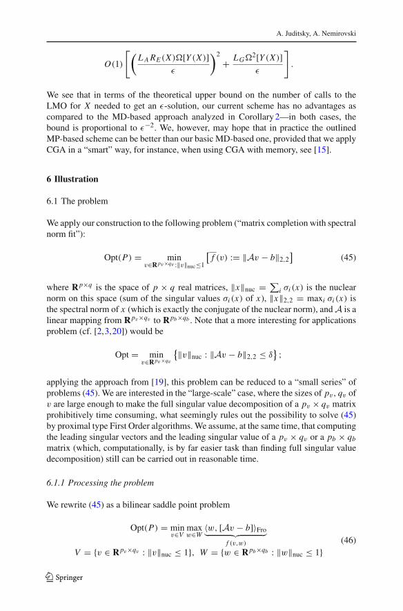
We apply our construction to the following problem (“matrix completion with spectralnorm fit”):

Opt(P) = minv∈R pv×qv :‖v‖nuc≤1

[f (v) := ‖Av − b‖2,2

](45)

where Rp×q is the space of p × q real matrices, ‖x‖nuc = ∑i σi (x) is the nuclear

norm on this space (sum of the singular values σi (x) of x), ‖x‖2,2 = maxi σi (x) isthe spectral norm of x (which is exactly the conjugate of the nuclear norm), and A is alinear mapping from Rpv×qv to Rpb×qb . Note that a more interesting for applicationsproblem (cf. [2,3,20]) would be

Opt = minv∈R pv×qv

{‖v‖nuc : ‖Av − b‖2,2 ≤ δ} ;

applying the approach from [19], this problem can be reduced to a “small series” ofproblems (45). We are interested in the “large-scale” case, where the sizes of pv, qv ofv are large enough to make the full singular value decomposition of a pv × qv matrixprohibitively time consuming, what seemingly rules out the possibility to solve (45)by proximal type First Order algorithms. We assume, at the same time, that computingthe leading singular vectors and the leading singular value of a pv × qv or a pb × qb

matrix (which, computationally, is by far easier task than finding full singular valuedecomposition) still can be carried out in reasonable time.

6.1.1 Processing the problem

We rewrite (45) as a bilinear saddle point problem

Opt(P) = minv∈V

maxw∈W

〈w, [Av − b]〉Fro︸︷︷︸f (v,w)

V = {v ∈ Rpv×qv : ‖v‖nuc ≤ 1}, W = {w ∈ Rpb×qb : ‖w‖nuc ≤ 1}(46)

123


(from now on 〈·, ·〉Fro stands for Frobenius inner product, and ‖·‖Fro – for the Frobeniusnorm on the space(s) of matrices). The domain X of the problem is the direct productof two unit nuclear norm balls; minimizing a linear form over this domain reduces tominimizing, given ξ and η, the linear forms Tr(vξ T ), Tr(wηT ) over {v ∈ Rpv×qv :‖v‖nuc ≤ 1}, resp., {w ∈ Rpb×qb : ‖w‖nuc ≤ 1}, which, in turn, reduces to computingthe leading singular vectors and singular values of ξ and η.

The monotone operator associated with (46) is affine and skew-symmetric:

�(v,w) = [∇v f (v,w);−∇w f (v,w)] = [A∗w;−Av]

+ [0; b] : R pv×qv × Rpb×qb︸︷︷︸

E

→ E .

From now on we assume that A is of spectral norm at most 1, i.e.,

‖Av‖Fro ≤ ‖v‖Fro, ∀v

(this always can be achieved by scaling).

Representing � We can represent the restriction of � on X by the data

F = Rpv×qv × Rpv×qv

Ay + a = [ξ ;Aη + b], y = [ξ ; η] ∈ F (ξ ∈ Rpv×qv , η ∈ R pv×qv ),

G([ξ ; η]︸︷︷︸

y

) = [−η; ξ ] : F → F

Y = {y = [ξ ; η] ∈ F : ‖ξ‖Fro ≤ 1, ‖η‖Fro ≤ 1}

(47)

Indeed, in the notation from Sect. 3.2, for x = [v;w] ∈ X = {[v;w] ∈ Rpv×qv ×Rpb×qb : ‖v‖nuc ≤ 1, ‖w‖nuc ≤ 1}, the solution y(x) = [ξ(x); η(x)] to the linearsystem A∗x = G(y) is given by η(x) = −v, ξ(x) = A∗w, so that both components ofy(x) are of Frobenius norm ≤ 1 (recall that spectral norm of A is ≤ 1), and thereforey(x) ∈ Y . Besides this,

Ay(x = [v;w])+ a = [ξ(x);Aη(x)+ b] = [A∗w; b − Av] = �(v,w).

We conclude that when x = [v;w] ∈ X , the just defined y(x) meets all requirementsfrom (7), and thus the data F, A, a, y(·),G(·), Y given by (47) indeed represent themonotone operator � on X .

The dual operator given by the data F, A, a, y(·),G(·), Y is

(

y︷︸︸︷[ξ ; η]) = A∗x(y)− G(y) = [v(y)+ η;A∗w(y)− ξ ],

v(y) ∈ Argmin‖v‖nuc≤1

〈v, ξ 〉, w(y) ∈ Argmin‖w‖≤1

〈w,Aη + b〉. (48)

Proximal setup We use the Euclidean proximal setup for Y , i.e., we equip the space Fembedding Y with the Frobenius norm and take, as the d.-g.f. for Y , the function

123


ω(ξ, η) = 1

2

[‖ξ‖2

Fro + ‖η‖2Fro

]: F := Rpv×qv × Rpv×qv → R,

resulting in �[Y ] = √2. Furthermore, from (48) and the fact that the spectral norm

of A is bounded by 1 it follows that the monotone operator�(y) = −(y) : Y → Fsatisfies (20) with M = 2

√2 and (26) with L = 0 and M = 4

√2.

Remark Theorem 1 combines with Corollary 1 to imply that when converting an accu-racy certificate CN for the dual v.i. VI(−,Y ) into a feasible solution x N to the primalv.i. VI(�, X), we ensure that

εsad (xN | f, V,W ) ≤ Res(CN |Y (X)) ≤ Res(CN |Y ), (49)

with f, V,W given by (46). In other words, in the representation x N = [vN ; wN ], vN

is a feasible solution to problem (45) (which is the primal problem associated with(46)), and wN is a feasible solution to the problem

Opt(D) = maxw∈W

minv∈V

〈w,Av − b〉 = maxw∈W

{f (w) := −‖A∗w‖2,2 − 〈b, w〉

},

(which is the dual problem associated with (46)) with the sum of non-optimalities,in terms of respective objectives, ≤ Res(CN |Y ). Computing f (w) (which, together

with computing f (v), takes a single call to LMO for X ), we get a lower bound onOpt(P) = Opt(D) which certifies that f (v)− Opt(P) ≤ Res(CN |Y ).

6.2 Numerical illustration

Here we report on some numerical experiments with problem (45). In these experi-ments, we used pb = qb =: m, pv = qv =: n, with n = 2m, and the mapping Agiven by

Av =k∑

i=1

�ivr Ti , (50)

with generated at random m × n factors �i , ri scaled to get ‖A‖∗ ≈ 1. In all ourexperiments, we used k = 2. Matrix b in (45) was built as follows: we generated atrandom n × n matrix v with ‖v‖nuc less than (and close to) 1 and Rank(v) ≈ √

n, andtook b = Av + δ, with randomly generated m × m matrix δ of spectral norm about0.01.

6.2.1 Experiments with the MD-based scheme

Implementing the MD-based scheme In the first series of experiments, the dual v.i.VI(−,Y ) is solved by the MD algorithm with N = 512 steps for all but the largestinstance, where N = 257 is used. The MD is applied to the stationary sequenceHt (·) ≡ −(·), t = 1, 2, . . ., of vector fields. The stepsizes γt are proportional, with

123


coefficient of order of 1, to those given by (21.b) with ‖ · ‖ ≡ ‖ · ‖∗ = ‖ · ‖Fro and�[Y ] = √

2;5 the coefficient was tuned empirically in pilot runs on small instancesand is never changed afterwards. We also use two straightforward “tricks”:

• Instead of considering one accuracy certificate, CN ={yt , λNt =1/N , −(yt )}N

t=1,we build a “bunch” of certificates

Cνμ ={

yt , λt = 1

ν − μ+ 1, −(yt )

}ν

t=μ,

where μ runs through a grid in {1, ..., N } (in this implementation, a 16-elementequidistant grid), and ν ∈ {μ,μ+ 1, . . . , N } runs through another equidistant grid(e.g., for the largest problem instance, the grid {1, 9, 17, . . . , 257}). We compute theresolutions of these certificates and identify the best (with the smallest resolution)certificate obtained so far. Every 8 steps, the best certificate is used to compute thecurrent approximate solution to (46) along with the saddle point inaccuracy of thissolution.

• When applying MD to problem (46), the “dual iterates” yt = [ξt ; ηt ] and the “pri-mal iterates” xt := x(yt ) = [vt ;wt ] are pairs of matrices, with n × n matricesξt , ηt , vt and m × m matrices wt (recall that we are in the case of pv = qv = n,pb = qb = m). It is easily seen that with A given by (50), the matrices ξt , ηt , vt arelinear combinations of rank 1 matrices αiβ

Ti , 1 ≤ i ≤ (k + 1)t , and wt are linear

combinations of rank 1 matrices δiεTi , 1 ≤ i ≤ t , with on-line computable vectors

αi , βi , δi , εi . Every step of MD adds k + 1 new α- and k + 1 new β-vectors, anda pair of new δ- and ε-vectors. Our matrix iterates were represented by the vectorsof coefficients in the above rank 1 decompositions (let us call this representationincremental), so that the computations performed at a step of MD, including com-puting the leading singular vectors by straightforward power iterations, are as ifthe standard representations of matrices were used, but all these matrices were ofthe size (at most) n × [(k + 1)N ], and not n × n and m × m, as they actually are.In our experiments, for k = 2 and N ≤ 512, this incremental representation ofiterates yields meaningful computational savings (e.g., by factor of 6 for n = 8192)as compared to the plain representation of iterates by 2D arrays.

Typical results of our preliminary experiments are presented in Table 1. There Ct standsfor the best certificate found in course of t steps, and Gap(Ct ) denotes the saddle pointinaccuracy of the solution to (46) induced by this certificate (so that Gap(Ct ) is a validupper bound on the inaccuracy, in terms of the objective, to which the problem ofinterest (45) was solved in course of t steps). The comments are as follows:

1. The computational results demonstrate “nearly linear”, and not quadratic, growthof running time with m, n; this is due to the incremental representation of iterates.

2. When evaluating the “convergence patterns” presented in the table, one shouldkeep in mind that we are dealing with a method with slow O(1/

√N ) convergence

5 As we have already mentioned, with our proximal setup, the ω-size of Y is ≤ √2, and (20) is satisfied

with M = 2√

2.

123


rate, and from this perspective, 50-fold reduction in resolution in 512 steps is notthat bad.

3. A natural alternative to the proposed approach would be to solve the saddle pointproblem (46) “as it is,” by applying to the associated primal v.i. (where the domainis the product of two nuclear norm balls and the operator is Lipschitz continuousand even skew symmetric) a proximal type saddle point algorithm and computingthe required prox-mappings via full singular value decompositions. The state-of-the-art MP algorithm when applied to this problem exhibits O(1/N ) convergencerate;6 yet, every step of this method would require 2 SVD’s of n × n, and 2SVD’s of m × m matrices. As applied to the primal v.i., MD exhibits O(1/

√N )

convergence rate, but the steps are cheaper—we need one SVD of n × n, and oneSVD of an m ×m matrix, and we are unaware of a proximal type algorithm for theprimal v.i. with cheaper iterations. For the sizes m, n, k we are interested in, thecomputational effort required by the outlined SVD’s is, for all practical purposes,the same as the overall effort per step. Taking into account the actual SVD cputimes on the platform used in our experiments, the overall running times presentedin Table 1, i.e., times required by 512 steps of MD as applied to the dual v.i., allowfor the following iteration counts N for MP as applied to the primal v.i.:

n 1024 2048 4096 8192N 406 72 17 4

and for twice larger iteration counts for MD. From our experience, for n = 1024(and perhaps for n = 2048 as well), MP algorithm as applied to the primal v.i.would yield solutions of better quality than those obtained with our approach.It, however, would hardly be the case, for both MP and MD, when n = 4096,and definitely would not be the case for n = 8192. Finally, with n = 16384,CPU time used by the 257-step MD as applied to the dual v.i. is hardly enough tocomplete just one iteration of MD as applied to the primal v.i. We believe thesedata demonstrate that the approach developed in this paper has certain practicalpotential.

6.2.2 Experiments with the MP-based scheme

In this section we briefly report on the results obtained with the modified MP-basedscheme presented in Sect. 5. Same as above, we use the test problems and represen-tation (47) of the monotone operator of interest (with the only difference that nowY = F), and the Euclidean proximal setup. Using the Euclidean setup on Y = Fmakes prox-mappings and functions fy(·), defined in (37), extremely simple:

Prox[ξ ;η]([dξ ; dη]) = [ξ − dξ ; η − dη] [ξ, dξ, η, dη ∈ Rpv×qv ]fy(x) = 1

2〈y − γ [Gy − A∗x], y − γ [Gy − A∗x]〉 + γ 〈a, x〉

6 For the primal v.i., (26) holds true for some L > 0 and M = 0. Moreover, with properly selected proximalsetup for (45) the complexity bound (28) becomes Res(CN |Y ) ≤ O(1)

√ln(n) ln(m)/N .

123


Tabl

e1

MD

onpr

oble

m(4

5)

Iter

atio

nco

untt

165

129

193

257

321

385

449

512

n=

1024

m=

512

k=

2

Res(C

t |Y)

1.54

020.

1535

0.08

860.

0621

0.04

870.

0389

0.03

288

0.02

930.

0278

Res(C

1|Y)/

Res(C

t |Y)

1.00

10.0

417.3

824.7

931.6

139.6

146.8

452.6

455.4

1

Gap(C

t )0.

1269

0.02

390.

0145

0.01

030.

0075

0.00

630.

0042

0.00

400.

0040

Gap(C

t )/G

ap(C

t )1.

005.

318.

7812.3

817.0

320.2

029.9

831.4

131.6

6

cpu,

sec

0.2

9.5

27.6

69.1

112.

621

8.1

326.

243

2.6

536.

4

n=

2048

m=

1024

k=

2

Res(C

t |Y)

1.48

090.

1559

0.08

420.

0607

0.04

710.

0391

0.03

370.

0306

0.02

85

Res(C

1|Y)/

Res(C

t |Y)

1.00

9.50

17.5

924.3

831.4

337.8

843.8

948.3

651.9

6

Gap(C

t )0.

1329

0.01

960.

0119

0.00

750.

0053

0.00

410.

0036

0.00

340.

0027

Gap(C

t )/G

ap(C

t )1.

006.

7911.2

117.8

125.0

932.2

937.2

338.7

050.0

6

cpu,

sec

0.7

38.0

101.

120

6.3

314.

150

8.9

699.

088

4.9

1070.0

n=

4096

m=

2048

k=

2

Res(C

t |Y)

1.48

450.

1476

0.08

910.

0605

0.04

910.

0395

0.03

290.

0292

0.02

75

Res(C

1|Y)/

Res(C

t |Y)

1.00

10.0

616.6

624.5

330.2

537.6

045.1

750.8

553.9

5

Gap(C

t )0.

1239

0.02

220.

0139

0.01

080.

0086

0.00

410.

0037

0.00

350.

0035

Gap(C

t )/G

ap(C

t )1.

005.

578.

9311.4

814.4

030.4

833.1

435.7

635.7

7

cpu,

sec

2.2

103.

525

7.6

496.

974

2.5

1147.8

1564.4

1981.4

2401.0

123


Tabl

e1

cont

inue

d

Iter

atio

nco

untt

165

129

193

257

321

385

449

512

n=

8192

m=

4096

k=

2

Res(C

t |Y)

1.47

780.

1391

0.08

880.

0590

0.04

690.

0386

0.03

240.

0289

0.02

70

Res(C

1|Y)/

Res(C

t |Y)

1.00

10.6

316.6

425.0

631.5

338.2

945.6

851.1

054.7

6

Gap(C

t )0.

1193

0.02

320.

0134

0.01

080.

0054

0.00

400.

0035

0.00

340.

0034

Gap(C

t )/G

ap(C

t )1.

005.

148.

9011.0

822.0

029.8

333.9

334.8

535.1

4

cpu,

sec

6.5

289.

968

3.8

1238.1

1816.0

2724.5

3648.3

4572.2

5490.8

n=

1638

4m

=81

92k

=2

Res(C

t )1.

4566

0.11

540.

0767

0.05

560.

0447

Res(C

1|Y)/

Res(C

t |Y)

1.00

12.6

219.0

026.2

232.6

0

Gap(C

t )0.

1195

90.

0213

60.

0146

00.

0101

10.

0085

3

Gap(C

t )/G

ap(C

t )1.

005.

608.

1911.8

214.0

1

cpu,

sec

21.7

920.

420

50.2

3492.4

4902.2

Plat

form

:3.4

0G

Hz

i7-3

770

desk

top

with

16G

BR

AM

,MA

TL

AB

Win

dow

s7

64

123


= 1

2

[‖ξ + γ η + γA∗w‖2

Fro + ‖η − γ ξ + γ v‖2Fro

]+ γ 〈b, w〉Fro

y = [ξ ; η], x = [v;w].

When choosing ‖ · ‖E to be the Frobenius norm,

‖ [v;w]︸︷︷︸

x

‖E = ‖x‖E,∗ =√

‖v‖2Fro + ‖w‖2

Fro

and taking into account that the spectral norm of A is ≤ 1, it is immediately seen thatthe quantities LG , L A and γ introduced in Sect. 5.2, can be set to 1, and what wascalled RE (X) in Sect. 5.2.2, can be set to

√2. As a result, by the complexity analysis of

Sect. 5.2.2, in order to find an ε-solution to the problem of interest, we need O(1)ε−1

iterations of the recurrence (35), with O(1)ε−1 CGA steps of minimizing fyt (·) overX per iteration, that is, the total of at most O(1)ε−2 calls to the LMO for X = V × W .In fact, in our implementation ε is not fixed in advance; instead, we fix the total numberN = 256 of calls to LMO, and terminate CGA at iteration t of the recurrence (35)when either a solution xt ∈ x with δt ≤ 0.1/t is achieved, or the number of CGAsteps reaches a prescribed limit (set to 32 in the experiment to be reported).

Same as in the first series of experiments, “incremental” representation of matrixiterates is used in the experiments with the MP-based scheme. In these experimentswe also use a special post-processing of the solution we explain next.Post-processing Recall that in the situation in question the step #i of the CGA atiteration #t of the MP-based recurrence produces a pair [vt,i ;wt,i ] of rank 1 n ×n andm×m matrices of unit spectral norm—the minimizers of the linear form 〈∇ fyt (xt,i ), x〉over x ∈ X ; here xt,i is i-th step of CGA minimization of fyt (·) over X . As a result,upon termination, we have at our disposal N = 256 pairs of rank one matrices [v j ;w j ],1 ≤ j ≤ N , known to belong to X . Note that the approximate solution x , as definedin Sect. 5.2.1, is a certain convex combination of these matrices. A natural way to geta better solution is to solve the optimization problem

Opt = minλ,v

{

f (λ) = ‖Av − b‖2,2 : v =∑N

j=1λ jv j ,

∑N

j=1|λ j | ≤ 1

}

. (51)

Indeed, note that the v-components of feasible solutions to this problem are of nuclearnorm ≤ 1, i.e., are feasible solutions to the problem of interest (45), and that in termsof the objective of (45), the v-component of an optimal solution to (51) can be onlybetter than the v-component of x . On the other hand, (51) is a low-dimensional convexoptimization problem on a simple domain, and the first order information on f canbe obtained, at a relatively low cost, by Power Method, so that (51) is well suited forsolving by proximal first order algorithms, e.g., the Bundle Level algorithm [21] weuse in our experiments.

Numerical illustration Here we present just one (in fact, quite representative) numer-ical example. In this example n = 4096 and m = 2048 (i.e., in (45) the variable matrixu is of size 4096 × 4096, and the data matrix b is of size 2048 × 2048); the map-ping A is given by (50) with k = 2. The data are generated in the same way as inthe experiments described in Sect. 6.2.1 except for the fact that we used b = Au to

123


ensure zero optimal value in (45). As a result, the value of the objective of (45) at anapproximate solution coincides with the inaccuracy of this solution in terms of theobjective of (45). In the experiment we report on here, the objective of (45) evaluatedat the initial – zero – solution, i.e., ‖b‖2,2, is equal to 0.751. After the total of 256 callsto the LMO for X [just 11 steps of recurrence (35)] and post-processing which took24% of the overall CPU time, the value of the objective is reduced to 0.013—by factor57.3. For comparison, when processing the same instance by the basic MD scheme,augmented by the just outlined post-processing, after 256 MD iterations (i.e., afterthe same as above 256 calls to the LMO), the value of the objective at the resultingfeasible solution to (45) was 0.071, meaning the progress in accuracy by factor 10.6(5 times worse than the progress in accuracy for the MP-based scheme). Keeping theinstance intact and increasing the number of MD iterations in the basic scheme from256 to 512, the objective at the approximate solution yielded by the post-processingreduces from 0.071 to 0.047, which still is 3.6 times worse than that achieved with theMP-based scheme after 256 calls to LMO.

7 Proofs

7.1 Proof of Theorems 1 and 2

We start with proving Theorem 2. In the notation of the theorem, we have

∀x ∈ X : �(x) = Ay(x)+ a,(a) : y(x) ∈ Y,(b) : 〈y(x)− y, A∗x − G(y(x))〉 ≥ 0 ∀y ∈ Y.

(52)

For x ∈ X , let y = y(x), and let y = ∑t λt yt , so that y, y ∈ Y by (52.a). Since G is

monotone, for all t ∈ {1, . . . , N } we have

〈y − yt ,G(y)− G(yt )〉 ≥ 0⇒ 〈y,G(y)〉 ≥ 〈yt ,G(y)〉 + 〈y,G(yt )〉 − 〈yt ,G(yt )〉 ∀t⇒ 〈y,G(y)〉 ≥ ∑

tλt [〈yt ,G(y)〉 + 〈y,G(yt )〉 − 〈yt ,G(yt )〉]

[since λt ≥ 0 and∑

tλt = 1],

and we conclude that

〈y,G(y)〉 − 〈y,G(y)〉 ≥N∑

t=1

λt [〈y,G(yt )〉 − 〈yt ,G(yt )〉] . (53)

We now have

〈�(x), x −∑

t

λt xt 〉

= 〈Ay + a, x −∑

t

λt xt 〉 = 〈y, A∗ x −∑

t

λt A∗xt 〉 + 〈a, x −∑

t

λt xt 〉

= 〈y, A∗ x − G(y)〉 + 〈y,G(y)−∑

t

λt A∗xt 〉 + 〈a, x −∑

t

λt xt 〉

123


≥ 〈y, A∗ x − G(y)〉 + 〈y,G(y)−∑

t

λt A∗xt 〉 + 〈a, x −∑

t

λt xt 〉

[by (52.b) with y = y and due to y = y(x)]= 〈y, A∗ x〉 + [〈G(y), y〉 − 〈G(y), y〉] − 〈y,

∑

t

λt A∗xt 〉 + 〈a, x −∑

t

λt xt 〉

≥ 〈y, A∗ x〉 +∑

t

λt [〈y,G(yt )〉 − 〈yt ,G(yt )〉] − 〈y,∑

t

λt A∗xt 〉

+〈a, x −∑

t

λt xt 〉 [by (53)]

=∑

t

λt 〈yt , A∗ x〉 +∑

t

λt[〈y,G(yt )〉 − 〈yt ,G(yt )〉 − 〈y, A∗xt 〉 + 〈a, x − xt 〉

]

[since y =∑

t

λt yt and∑

t

λt = 1]

=∑

t

λt [〈Ayt , x − xt 〉 + 〈Ayt , xt 〉 + 〈y,G(yt )〉 − 〈yt ,G(yt )〉

−〈y, A∗xt 〉 + 〈a, x − xt 〉]

=∑

t

λt[〈yt , A∗xt 〉 + 〈y,G(yt )〉 − 〈yt ,G(yt )〉 − 〈y, A∗xt 〉

]

+∑

t

λt 〈Ayt + a, x − xt 〉

=∑

tλt 〈A∗xt − G(yt ), yt − y〉 +

∑

t

λt 〈Ayt + a, x − xt 〉 ≥ −ε

+∑

t

λt 〈Ayt + a, x − xt 〉

[by(15) due toy = y(x) ∈ Y (X)].

The bottom line is that

〈�(x), x − x〉 ≤ ε +N∑

t=1

λt 〈Ayt + a, xt − x〉 ∀x ∈ X,

as stated in (16). Theorem 2 is proved.To prove Theorem 1, let yt ∈ Y , 1 ≤ t ≤ N , and λ1, . . . , λN be from the premise

of the theorem, and let xt , 1 ≤ t ≤ N , be specified as xt = x(yt ), so that xt is theminimizer of the linear form 〈Ayt + a, x〉 over x ∈ X . Due to the latter choice, wehave

∑Nt=1 λt 〈Ayt +a, xt − x〉 ≤ 0 for all x ∈ X , while ε as defined by (15) is nothing

but Res({yt , λt ,−(xt )}Nt=1|Y (X)). Thus, (16) in the case in question implies that

∀x ∈ X : 〈�(x),N∑

t=1

λt xt − x〉 ≤ Res({yt , λt ,−(xt )}Nt=1|Y (X)),

and (13) follows. Relation (14) is an immediate corollary of (13) and Lemma 2 asapplied to X in the role of Y , � in the role of H(·), and {xt , λt ,�(xt )}N

t=1 in the roleof CN . ��

123


7.2 Proof of Proposition 1

Observe that the optimality conditions in the optimization problem specifying v =Proxy(ξ) imply that

〈ξ − ω′(y)+ ω′(v), z − v〉 ≥ 0, ∀z ∈ Y,

or

〈ξ, v − z〉 ≤ 〈ω′(v)− ω′(y), z − v〉 = 〈V ′y(v), z − v〉, ∀z ∈ Y,

which, using a remarkable identity [5]

〈V ′y(v), z − v〉 = Vy(z)− Vv(z)− Vy(v),

can be rewritten equivalently as

v = Proxy(ξ) ⇒ 〈ξ, v − z〉 ≤ Vy(z)− Vv(z)− Vy(v) ∀z ∈ Y. (54)

Setting y = yt , ξ = γt Ht (yt ), which results in v = yt+1, we get

∀z ∈ Y : γt 〈Ht (yt ), yt+1 − z〉 ≤ Vyt (z)− Vyt+1(z)− Vyt (yt+1),

whence,

∀z ∈ Y : γt 〈Ht (yt ), yt − z〉 ≤ Vyt (z)−Vyt+1(z)+[γt 〈Ht (yt ), yt − yt+1〉−Vyt (yt+1)

]

︸︷︷︸≤γt ‖Ht (yt )‖∗‖yt −yt+1‖− 1

2 ‖yt −yt+1‖2

≤ Vyt (z)− Vyt+1(z)+ 1

2γ 2

t ‖Ht (yt )‖2∗.

Summing up these inequalities over t = 1, . . . , N and taking into account that forz ∈ Y ′, we have Vy1(z) ≤ 1

2�2[Y ′] and that VyN+1(z) ≥ 0, we get (19). ��

7.3 Proof of Proposition 2

Applying (54) to y = yt , ξ = γt Ht (zt ), which results in v = yt+1, we get

∀z ∈ Y : γt 〈Ht (zt ), yt+1 − z〉 ≤ Vyt (z)− Vyt+1(z)− Vyt (yt+1),

whence, by the definition (23) of dt ,

∀z ∈ Y : γt 〈Ht (zt ), zt − z〉 ≤ Vyt (z)− Vyt+1(z)+ dt . (55)

123


Summing up the resulting inequalities over t = 1, . . . , N and taking into account thatVy1(z) ≤ 1

2�2[Y ′] for all z ∈ Y ′ and VyN+1(z) ≥ 0, we get

∀z ∈ Y ′ :n∑

t=1

λNt 〈Ht (zt ), zt − z〉 ≤

12�

2[Y ′] + ∑Nt=1 dt

∑Nt=1 γt

.

The right hand side in the latter inequality is independent of z ∈ Y ′. Taking supremumof the left hand side over z ∈ Y ′, we arrive at (24).

Moreover, invoking (54) with y = yt , ξ = γt Ht (yt ) and specifying z as yt+1, weget

γt 〈Ht (yt ), zt − yt+1〉 ≤ Vyt (yt+1)− Vzt (yt+1)− Vyt (zt ),

whence

dt = γt 〈Ht (zt ), zt − yt+1〉 − Vyt (yt+1) ≤ γt 〈Ht (yt ), zt − yt+1〉+ γt 〈Ht (zt )− Ht (yt ), zt − yt+1〉 − Vyt (yt+1)

≤ −Vzt (yt+1)− Vyt (zt )+ γt 〈Ht (zt )− Ht (yt ), zt − yt+1〉≤ γt‖Ht (zt )− Ht (yt )‖∗‖zt − yt+1‖ − 1

2‖zt − yt+1‖2 − 1

2‖yt − zt‖2

≤ 1

2

[γ 2

t ‖Ht (zt )− Ht (yt )‖2∗ − ‖yt − zt‖2],

(56)

as required in (25). ��

7.4 Proof of Lemma 3

10. We start with the following standard fact:

Lemma 4 Let Y be a nonempty closed convex set in Euclidean space F, ‖ · ‖ be anorm on F, and ω(·) be a continuously differentiable function on Y which is stronglyconvex, modulus 1, w.r.t. ‖ · ‖. Given b ∈ F and y ∈ Y , let us set

gy(ξ) = maxz∈Y

[〈z, ω′(y)− ξ 〉 − ω(z)] : F → R,

Proxy(ξ) = argmaxz∈Y

[〈z, ω′(y)− ξ 〉 − ω(z)].

The function gy is convex with Lipschitz continuous gradient ∇gy(ξ) = − Proxy(ξ):

‖∇gy(ξ)− ∇gy(ξ′)‖ ≤ ‖ξ − ξ ′‖∗ ∀ξ, ξ ′, (57)

where ‖ · ‖∗ is the norm conjugate to ‖ · ‖.

123


Indeed, since ω is strongly convex and continuously differentiable on Y , Proxy(·) iswell defined, and from optimality conditions it holds

〈ω′(Proxy(ξ))+ ξ − ω′(y),Proxy(ξ)− z〉 ≤ 0 ∀z ∈ Y. (58)

Consequently, gy(·) is well defined; this function clearly is convex, and the vector− Proxy(ξ) clearly is a subgradient of gy at ξ . If now ξ ′, ξ ′′ ∈ F , then, setting z′ =Proxy(ξ

′), z′′ = Proxy(ξ′′) and invoking (58), we get

〈ω′(z′)+ ξ ′ − ω′(y), z′ − z′′〉 ≤ 0, 〈−ω′(z′′)− ξ ′′ + ω′(y), z′ − z′′〉 ≤ 0

whence, summing the inequalities up,

〈ξ ′ − ξ ′′, z′ − z′′〉 ≤ 〈ω′(z′)− ω′(z′′), z′′ − z′〉 ≤ −‖z′ − z′′‖2,

implying that ‖z′ − z′′‖ ≤ ‖ξ ′ − ξ ′′‖∗. Thus, a subgradient field − Proxy(·) of gy(·) isLipschitz continuous with constant 1 from ‖ · ‖∗ into ‖ · ‖, whence gy is continuouslydifferentiable and (57) takes place. ��20. To derive Lemma 3 from Lemma 4, note that fy(x) is obtained from gy(·) by affinesubstitution of variables and adding linear form:

fy(x) = gy(γ [G(y)− A∗x])+ γ 〈a, x〉+ω(y)− 〈ω′(y), y〉.

whence ∇ fy(x) = −γ A∇gy(γ [G(y)− A∗x])+γ a = γ A Proxy(γ [G(y)− A∗x])+γ a, as required in (39), and

‖∇ fy(x′)− ∇ fy(x

′′)‖E,∗= γ ‖A

[∇gy(γ [G(y)− A∗x ′])− ∇gy(γ [G(y)− A∗x ′′])] ‖E,∗≤ (γ L A)‖∇gy(γ [G(y)− A∗x ′])− ∇gy(γ [G(y)− A∗x ′′])‖≤ (γ L A)‖γ [G(y)− A∗x ′] − γ [G(y)− A∗x ′′]‖∗≤ (γ L A)

2‖x ′ − x ′′‖E = (L A/LG)2‖x ′ − x ′′‖E

[we have used (57) and equivalences in (38)], as required in (40). ��

7.5 Review of Conditional Gradient algorithm

The required description of CGA and its complexity analysis are as follows.As applied to minimizing a smooth – with Lipschitz continuous gradient

‖∇ f (u)− ∇ f (u′)‖E,∗ ≤ L‖u − u′‖E , ∀u, u′ ∈ X,

123


convex function f over a convex compact set X ⊂ E , the generic CGA is the recurrenceof the form

u1 ∈ Xus+1 ∈ X satisfies f (us+1) ≤ f (us + γs[u+

s − us]), s = 1, 2, . . .γs = 2

s+1 , u+s ∈ Argmin u∈X 〈 f ′(us), u〉.

The standard results on this recurrence (see, e.g., proof of Theorem 1 in [15]) statethat if f∗ = minX f , then

(a) εt+1 := f (ut+1)− f∗ ≤ εt − γtδt + 2LR2γ 2t , t = 1, 2, ...

δt := maxu∈X 〈∇ f (ut ), ut − u〉;(b) εt ≤ 2LR2

t+1 , t = 2, 3, . . .(59)

where R is the smallest of the radii of ‖ ·‖E -balls containing X . From (59.a) it followsthat

γτ δτ ≤ ετ − ετ+1 + 2LR2γ 2τ , τ = 1, 2, . . . ;

summing up these inequalities over τ = t, t + 1, . . . , 2t , where t > 1, we get

[

minτ≤2t

δτ

] 2t∑

τ=t

γτ ≤ εt + 2LR22t∑

τ=t

γ 2τ ,

which combines with (59.b) to imply that

minτ≤2t

δτ ≤ O(1)LR21t + ∑2t

τ=t1τ 2

∑2tτ=t

1τ

≤ O(1)LR2

t.

It follows that given ε < LR2, it takes at most O(1)LR2

εsteps of CGA to generate a

point uε ∈ X with maxu∈X 〈∇ f (uε), uε − u〉 ≤ ε.

References

1. Beck, A., Teboulle, M.: Mirror descent and nonlinear projected subgradient methods for convex opti-mization. Oper. Res. Lett. 31(3), 167–175 (2003)

2. Candes, E.J., Plan, Y.: Matrix completion with noise. Proc. IEEE 98(6), 925–936 (2010)3. Candes, E.J., Plan, Y.: Tight oracle inequalities for low-rank matrix recovery from a minimal number

of noisy random measurements. Inf. Theory IEEE Trans. 57(4), 2342–2359 (2011)4. Castellani, M., Mastroeni, G.: On the duality theory for finite dimensional variational inequalities. In:

Giannessi, F., Maugeri, A. (eds.) Variational Inequalities Network Equilibrium Problems, pp. 21–31.Plenum Publishing, New York (1995)

5. Chen, G., Teboulle, M.: Convergence analysis of a proximal-like minimization algorithm using Breg-man functions. SIAM. J. Optim. 3(3), 538–543 (1993)

6. Chipot, M.: Variational Inequalities and Flow in Porous Media. Springer, New York (1984)7. Cox, B., Juditsky, A., Nemirovski, A.: Dual subgradient algorithms for large-scale nonsmooth learning

problems. Math. Program. Ser. B 148(1–2), 143–180 (2014)

123


8. Daniele, P.: Dual variational inequality and appluications to asymmetric traffic equalibrium probnlemswith capacity constraints. Le Mathematiche XLIX(2), 111–211 (1994)

9. Demyanov, V., Rubinov, A.: Approximate Methods in Optimization Problems. Elsevier, Amsterdam(1970)

10. Dunn, J.C., Harshbarger, S.: Conditional gradient algorithms with open loop step size rules. J. Math.Anal. Appl. 62(2), 432–444 (1978)

11. Dudik, M., Harchaoui, Z., Malick, J.: Lifted coordinate descent for learning with trace-norm regular-ization. In: AISTATS-Proceedings of the Fifteenth International Conference on Artificial Intelligenceand Statistics, vol. 22, pp. 327–336 (2012)

12. Frank, M., Wolfe, P.: An algorithm for quadratic programming. Naval Res. Logist. Q. 3(1–2), 95–110(1956)

13. Freund, R., Grigasy. P.: New analysis and results for the Conditional Gradient method (2013) submittedto Mathematical Programming, E-print: http://web.mit.edu/rfreund/www/FW-paper-final

14. Harchaoui, Z., Douze, M., Paulin, M., Dudik, M., Malick, J.: Large-scale image classification withtrace-norm regularization. In: 2012 IEEE Conference on Computer Vision and Pattern Recognition(CVPR), pp. 3386–3393 (2012)

15. Harchaoui, Z., Juditsky, A., Nemirovski, A.: Conditional Gradient algorithms for norm-regularizedsmooth convex optimization. Mathematical Programming. Online First (2014). doi:10.1007/s10107-014-0778-9. E-print: arXiv:1302.2325

16. Jaggi, M.: Revisiting Frank–Wolfe: projection-free sparse convex optimization. In: Proceedings of the30th International Conference on Machine Learning (ICML 2013), pp. 427–435 (2013)

17. Jaggi, M., Sulovsky, M.: A simple algorithm for nuclear norm regularized problems. In: Proceedingsof the 27th International Conference on Machine Learning (ICML 2010), pp. 471–478 (2010)

18. Juditsky, A., Nemirovski, A.: First order methods for nonsmooth large-scale convex minimization, I:general purpose methods; II: utilizing problem’s structure. In: Sra, S., Nowozin, S., Wright, S. (eds.)Optimization for Machine Learning, pp. 121–184. The MIT Press, Cambridge (2012)

19. Juditsky, A., Kilinç Karzan, F., Nemirovski, A.: Randomized first order algorithms with applicationsto �1-minimization. Math. Program. Ser. A 142(1–2), 269–310 (2013)

20. Juditsky, A., Kilinç Karzan, F., Nemirovski, A.: On unified view of nullspace-type conditions forrecoveries associated with general sparsity structures. Linear Algebra Appl. 441(1), 124–151 (2014)

21. Lemarechal, C., Nemirovski, A., Nesterov, Yu.: New variants of bundle methods. Math. Program.69(1), 111–148 (1995)

22. Mosco, U.: Dual variational inequalities. J. Math. Anal. Appl. 40, 202–206 (1972)23. Nemirovski, A., Yudin, D.: Problem Complexity and Method Efficiency in Optimization. Nauka Pub-

lishers, Moscow (1978) (in Russian); John Wiley, New York (1983) (in English)24. Nemirovskii, A.: Efficient iterative algorithms for variational inequalities with monotone operators.

Ekonomika i Matematicheskie Metody 17(2), 344–359 (1981). (in Russian; Engllish translation:Matekon)

25. Nemirovski, A.: Prox-method with rate of convergence O(1/t) for variational inequalities with Lip-schitz continuous monotone operators and smooth convex-concave saddle point problems. SIAM J.Optim. 15, 229–251 (2004)

26. Nemirovski, A., Onn, S., Rothblum, U.: Accuracy certificates for computational problems with convexstructure. Math. Oper. Res. 35, 52–78 (2010)

27. Nesterov, Yu., Nemirovski, A.: On first order algorithms for �1/nuclear norm minimization. ActaNumer. 22, 509–575 (2013)

28. Pshenichnyi, B.N., Danilin, Y.M.: Numerical Methods in Extremal Problems. Mir Publishers, Moscow(1978)

29. Rockafellar, R.T.: Minimax theorems and conjugate saddle functions. Math. Scand. 14, 151–173 (1964)30. Rockafellar, R.T.: Convex Analysis. Princeton University Press, Princeton (1970)31. Shalev-Shwartz, S., Gonen, A., Shamir, O.: Large-scale convex minimization with a low-rank constraint

(2011). E-print: arXiv:1106.1622

123

http://web.mit.edu/rfreund/www/FW-paper-final

http://dx.doi.org/10.1007/s10107-014-0778-9

http://dx.doi.org/10.1007/s10107-014-0778-9

http://arxiv.org/abs/1302.2325

http://arxiv.org/abs/1106.1622

arkadi nemirovski - isyenemirovs/judnemlmo2015.pdf · math. program., ser. a doi...

Documents