armenta dis
TRANSCRIPT
7/23/2019 Armenta Dis
http://slidepdf.com/reader/full/armenta-dis 1/263
MECHANISMS AND CONTROL OF WATER INFLOW TO WELLS IN GAS
RESERVOIRS WITH BOTTOM-WATER DRIVE
A Dissertation
Submitted to the Graduate Faculty of the
Louisiana State University andAgricultural and Mechanical College
in Partial fulfillment of the
requirements for the degree of
Doctor of Philosophy
in
The Craft & Hawkins Department of Petroleum Engineering
by
Miguel Armenta
B.S. Petroleum Engineering, Universidad Industrial de Santander, Colombia, 1985
M. Environmental Development, Pontificia Universidad Javeriana, Colombia, 1996
December 2003

7/23/2019 Armenta Dis
http://slidepdf.com/reader/full/armenta-dis 2/263
ACKNOWLEDGMENTS
To God, my best and inseparable friend, for you are the glory, honor and
recognition.
To my wife, Chechy, and my children Andrea and Miguel, for giving me so much
love and support. Without you, getting this important step in my life, my PhD, has no
meaning. You are my inspiration and my strength.
To my parents, El Viejo Migue and La Niña Dorita, you are my source of beliefs.
You taught and gave me the determination and tools to reach my dreams with honesty
and hard work.
To my advisor, Dr. Andrew Wojtanowicz, for his guidance and challenging
comments. Without that motivation, this research would have been poor; however, facing
the challenges four different technical papers have been already published and presented
from this research.
To Dr. Christopher White for helping me with such honesty and unselfishness.
You were my lifesaver at my hardest time during my research. I knew I could always
count on you.
To Dr. Zaki Bassiouni, chairman of the Craft & Hawking Petroleum Engineering
Department, for giving me the right comments and advise at the right time.
To the rest of Craft & Hawking Petroleum Engineering Department faculty
members, Dr. John Smith, Dr. Julius Langlinais, Dr. Dandina Rao, and Dr. John
McMullan, from each one of you I learned many important things not only for my
professional life, but also for my personal life. I will always have you in my mind and
heart.
ii
7/23/2019 Armenta Dis
http://slidepdf.com/reader/full/armenta-dis 3/263
To my friends in Baton Rouge: Patricio & Maquica, Jose & Ericka, Juan &
Joanne, Fernando & Sabina, Jaime & Luz Edith, Alvaro & Tonya, Doña Luz & Dr.
Narses, Jorge & Ana Maria, Nicolas & Solange, and La Pili. All of you are angels sent by
God to help me during my crisis-time; you, however, did not know your mission. God
bless you.
iii

7/23/2019 Armenta Dis
http://slidepdf.com/reader/full/armenta-dis 4/263
TABLE OF CONTENTS
ACKNOWLEDGEMENTS….…………………………………………………………ii
LIST OF TABLES……………………………………………………………………..vii
LIST OF FIGURES..…………………………………………………………………..viii
NOMENCLATURE.…………….…………………………………………………….xiv
ABSTRACT…………………….……………………………………………………..xvii
CHAPTER 1 INTRODUCTION ………………………………………………………1
1.1 Background and Purpose……………………...…………………………………..1
1.2 Statement of Research Problem………………...…..……………………………..41.3 Significance and Contribution of this Research.…………………………………..5
1.4 Research Method and Approach……………....…………………………………..61.5 Work Program Logic………………………….…………………………………..8
CHAPTER 2 LITERATURE REVIEW……………………………………………...11
2.1 Critical Velocity………………………………………………………………….11
2.2 Critical Rate for Water Coning………………………………….……………….132.3 Techniques Used in Solving Water Loading ……………………………………16
2.3.1 Tubing Lift Improvement..………………………………………………16
2.3.1.1. Chemical Injection….…………………………………………162.3.1.2. Physical Modification…..……………………………………..18
2.3.1.3. Thermal…………..……………………………………………192.3.1.4. Mechanical. ….…..……………………………………………20
2.3.2 Bottom Liquid Removal...………………………………………………21
2.3.2.1. Pumps………….………………………………………………222.3.2.2. Swabbing………………………………………………………23
2.3.2.3. Plungers…………………………………..……………………24
2.3.2.4. Downhole Gas Water Separation……………………….……..27
CHAPTER 3 MECHANISTIC COMPARISON OF WATER CONING IN OIL
AND GAS WELLS…………..…………………………………………30
3.1 Vertical Equilibrium.………………………………...…………………………..303.2 Analytical Comparison of Water Coning in Oil and Gas Wells before Water
Breakthrough ………………………………………...…………………………..31
3.3 Analytical Comparison of Water Coning in Oil and Gas Wells after WaterBreakthrough ………………………………………...…………………………..32
3.4 Numerical Simulation Comparison of Water Coning in Oil and Gas Wells after
Water Breakthrough …………….…………………...…………………………..373.5 Discussion about Water Coning in Oil-Water and Gas-Water Systems..………..41
CHAPTER 4 EFFECTS INCREASING BOTTOM WATER INFLOW TO GAS
WELLS………....…………...…………………………………..………43
4.1 Effect of Vertical Permeability…………………...…………….………………..44
iv

7/23/2019 Armenta Dis
http://slidepdf.com/reader/full/armenta-dis 5/263
4.2 Aquifer Size Effects..………………..…..………...………..…….……………..47
4.3 Non-Darcy Flow Effect..…………………………………………….…………..494.3.1 Analytical Model………………..…….………………….….…………..50
4.3.2 Numerical Model………………..…….………………….….…………..55
4.4 Effect of Perforation Density……………………..……...……………….……...57
4.5 Effect of Flow behind Casing …………………….……...……………….……..584.5.1 Cement Leak Model….…………..…….………………….……………..59
4.5.1.1 Effect of Leak Size and Length………………………………….64
4.5.1.2 Diagnosis of Gas Well with Leaking Cement…………..……….67
CHAPTER 5 EFFECT OF NON-DARCY FLOW ON WELL PRODUCTIVITY
IN TIGHT GAS RESERVOIRS…….………………………..………69
5.1 Non-Darcy Flow Effect in Low-Rate Gas Wells……………….………………..70
5.2 Field Data Analysis…………………………….……………….………………..73
5.3 Numerical Simulator Model…..……………….……………….………………..765.3.1 Volumetric Gas Reservoir………..…….………………….……………..78
5.3.2 Water Drive Gas Reservoir………..…….………………….………..…..805.4 Results and Discussion………..……………….……………….………………..85
CHAPTER 6 WELL COMPLETION LENGTH OPTIMIZATION IN GAS
RESERVOIRS WITH BOTTOM WATER ………..………..……….87
6.1 Problem Statement……………………….………………….….………………..876.2 Study Approach…..…….…………..……………………….….………………..88
6.2.1 Reservoir Simulation Model……………………………………………..88
6.2.1.1 Factors Considered…………………………………………………..896.2.1.2 Responses Considered…………………………………………….…90
6.2.2 Statistical Methods…………………………………………………….…916.2.2.1 Experimental Design…………………………………………………91
6.2.2.2 Statistical Analyses…………………………………………………..91
6.2.2.3 Linear Regression Models…………………………………………...926.2.2.4 Analysis of Variance…………………………………………………93
6.2.2.5 Monte Carlo Simulation……………………………………………..93
6.2.3 Optimization……………………………………………………………..94
6.2.4 Workflow………………………………………………………………...946.3 Results and Discussion…………………………………………………………..96
6.3.1 Linear Models……………………………………………………………96
6.3.2 Sensitivities (ANOVA)…………………………………………………..986.3.3 Monte Carlo Simulation………………………………………………...103
6.3.4 Optimization……………………………………………………………107
6.4 Implications For Water-Drive Gas Wells………………………………………108
CHAPTER 7 DOWNHOLE WATER SINK WELL COMPLETIONS IN GAS
RESERVOIR WITH BOTTOM WATER….………………...……..110
7.1 Alternative Design of DWS for Gas Wells…………………….……………….110
7.1.1 Dual Completion without Packer..…….………………….…………….111
7.1.2 Dual Completion with Packer…...…….………………….…………….112
7.1.3 Dual Completion with a Packer and Gravity Gas-WaterSeparation………………………..…….………………….……………113
v
7/23/2019 Armenta Dis
http://slidepdf.com/reader/full/armenta-dis 6/263
7.2 Comparison of Conventional Wells and DWS Wells.………….………………115
7.2.1 Reservoir Simulator Model……...…….………………….…………….1157.2.2 Reservoir Parameters Selection…..…….………………….…………...117
7.2.3 Conventional Wells Completion Length…...…………….…………….118
7.2.4 Gas Recovery and Production Time Comparison..……….…………….122
7.2.5 Reservoir Candidates for DWS Application……..……….…………….1247.3 Comparison of DWS and DGWS………………………..…….……………….126
7.3.1 DWS and DGWS Simulation Model….………………….…………….126
7.3.2 DWS vs. DGWS Comparison Results ..………………….…………….1277.3.3 Discussion About the Packer for DWS Wells...………….…………….131
CHAPTER 8 DESIGN AND PRODUCTION OF DWS GAS WELLS.…..……...133
8.1 Effect of Top Completion Length………………………….….………………..134
8.2 Effect of Water-Drainage Rate from the Bottom Completion……..….………..137
8.3 Effect of Separation between the Two Completions.……….….………………1398.4 Effect of Bottom Completion Length………………………….….…………....141
8.5 DWS Operational Conditions for Gas Wells…………….….………………….1438.5.1 Effect of Bottom Hole Flowing Pressure at the Bottom
Completion….………….………………………………….…………...1498.6 When to Install DWS in Gas Wells…………….….……………..…………….153
8.7 Recommended DWS Operational Conditions in Gas Wells……….….……….156
CHAPTER 9 CONCLUSIONS AND RECOMMENDATIONS….………...……..158
9.1 Conclusions………………………..……………………….….………………..158
9.2 Recommendations..………………..……………………….….………………..161
REFERENCES……………………….………………………………………………..163
APPENDIX-A ANALYTICAL COMPARISON OF WATER CONING IN OIL
AND GAS WELLS……….…………..……………………………..175
APPENDIX-B EXAMPLE ECLIPSE DATA DECK FOR COMPARISON OF
WATER CONING IN OIL AND GAS WELLS AFTER WATER
BREAKTHROUGH ………………………………………………..181
APPENDIX-C EXAMPLE ECLIPSE DATA DECK FOR EFFECT OF
VERTICAL PERMEABILITY ON WATER CONING..………..190
APPENDIX-D ANALYTICAL MODEL FOR NON-DARCY EFFECT IN LOW
PRODUCTIVITY GAS RESERVOIRS……………….....………..213
APPENDIX-E EXAMPLE IMEX DATA DECK FOR NON-DARCY FLOW IN
LOW PRODUCTIVITY GAS RESERVOIRS..…..……..………..215
APPENDIX-F EXAMPLE ECLIPSE DATA DECK FOR COMPARISON OF
CONVENTIONAL WELLS AND DWS WELLS..……..………...227
VITA…………………………………………………………….……..……..………..245
vi

7/23/2019 Armenta Dis
http://slidepdf.com/reader/full/armenta-dis 7/263
LIST OF TABLES
Table 3.1 Gas, Water, and Oil Properties Used for the Numerical Simulator Model…...38
Table 5.1 Data Used for the Analytical Model…………………………………………..71
Table 5.2 Rock Properties and Flow Rates Data for Wells A-6, A-7, and A-8 from Brar
& Aziz (1978)…………….……………………………………………………74
Table 5.3 Flow Rate and Values of a and b for Gas Wells with Multi-flow Tests….…...75
Table 5.4 Gas and Water Properties Used for the Numerical Simulator Model…………77
Table 6.1 Factor Descriptions……………………………………………………………89
Table 6.2 Factor Descriptions Including Box-Tidwell Power Coefficients……………..97
Table 6.3 Linear Sensitivity Estimates For Models Without Factors Interactions….…..99
Table 6.4 Transformed, Scaled Model for the Box-Cox Transform of Net Present
Value………………………………………………………………….…….100
Table 6.5 Parameters for Beta Distributions of Factors………………………….……..104
Table 6.6 Monte Carlo Sensitivity Estimates…………………………………………..105
Table 8.1 Operation Conditions for Top Completion Length Evaluation….…………..136
Table 8.2 Operation Conditions for Water-Drained Rate Evaluation……….………….137
Table 8.3 Operation Conditions for Evaluation of Separation Between The
Completions………………………………………………………….……..139
Table 8.4 Operation Conditions for Different Bottom Completion Length……….…...142
Table 8.5 Operation Conditions for Different Top Completion Length, BottomCompletion Length, and Water-Drained Rate…….……..…….…………...145
Table 8.6 Operation Conditions for Evaluation of Different Constant BottomholeFlowing Pressure at The Bottom Completion………………………………149
Table 8.7 Operation Conditions for “When” to Install DWS in Low Productivity GasWell…………..………………………………………….………………….153
vii

7/23/2019 Armenta Dis
http://slidepdf.com/reader/full/armenta-dis 8/263
LIST OF FIGURES
Figure 1.1 Gas Rate and Water Rate History for an Actual Gas Well……………………2
Figure 1.2 Gas Recovery Factor and Water Rate History for an Actual Gas Well……….2
Figure 3.1 Theoretical Model Used to Compare Analytically Water Coning in Oil and
Gas Wells before Breakthrough..………..…………………………………...31
Figure 3.2 Theoretical Model Used to Compare Analytically Water Coning in Oil and
Gas Wells after Breakthrough….....…….……………………………….…...33
Figure 3.3 Shape of the Gas-Water and Oil-Water Contact for Total Perforation.……...36
Figure 3.4 Numerical Model Used for Comparison of Water Coning in Oil-Water and
Gas-Water Systems……..…………………………………………….……...37
Figure 3.5 Numerical Comparison of Water Coning in Oil-Water and Gas-Water
Systems after 395 Days of Production………….…………………….……...39
Figure 3.6 Zoom View around the Wellbore to Watch Cone Shape for the Numerical
Model after 395 Days of Production….………..…………………….….…...40
Figure 4.1 Numerical Reservoir Model Used to Investigate Mechanisms ImprovingWater Coning/Production (Vertical Permeability and Aquifer Size)….….....44
Figure 4.2 Distribution of Water Saturation after 395 days of Gas Production…….…...45
Figure 4.3 Water Rate versus Time for Different Values of Permeability Anisotropy....46
Figure 4.4 Distribution of Water Saturation after 1124.8 days of Gas Production……..48
Figure 4.5 Water Rate versus Time for Different Values of Aquifer Size……………...49
Figure 4.6 Analytical Model Used to Investigate the Effect of Non-Darcy in Water
Production…..………..……………………………………………………...50
Figure 4.7 Skin Components at the Well for a Single Perforation for the Analytical
Model Used to Investigate Non-Darcy Flow Effect in Water Production…...52
Figure 4.8 Water-Gas Ratio versus Gas Recovery Factor for Total Penetration of Gas
Column without Skin and Non-Darcy Effect………..………..….……….…53
Figure 4.9 Water-Gas Ratio versus Gas Recovery Factor for Total Penetration of GasColumn Including Mechanical Skin Only…………..…………..…………...53
viii

7/23/2019 Armenta Dis
http://slidepdf.com/reader/full/armenta-dis 9/263
Figure 4.10 Water-Gas Ratio versus Gas Recovery Factor for Total Penetration of Gasand Water Columns, Skin and Non-Darcy Effect Included……...…..……...54
Figure 4.11 Water-Gas Ratio versus Gas Recovery Factor for Wells Completed Only
through Total Perforation the Gas Column with Combined Effects of Skinand Non-Darcy……..……………………..……..…………..……….……...55
Figure 4.12 Gas Rate versus Time for the Numerical Model Used to Evaluate the Effectof Non-Darcy Flow in Water Production……..……………………………...56
Figure 4.13 Water Rate versus Time for the Numerical Model Used to Evaluate theEffect of Non-Darcy Flow in Water Production……..……………………....57
Figure 4.14 Effect of Perforation Density on Water-Gas Ratio for a Well Perforating inthe Gas Column, Skin and Non-Darcy Effect Included..…………….……....58
Figure 4.15 Cement Channeling as a Mechanism Enhancing Water Production in Gas
Wells………..……………………………..………………………………....59
Figure 4.16 Modeling Cement Leak in Numerical Simulator ……..…………………....60
Figure 4.17 Relationship between Channel Diameter and Equivalent Permeability in the
First Grid for the Leaking Cement Model……..………………………….....62
Figure 4.18 Values of Radial and Vertical Permeability in the Simulator’s First Grid to
Represent a Channel in the Cemented Annulus.……..…………….….….....63
Figure 4.19 Effect of Leak Length: Behavior of Water Production Rate with and
without a Channel in the Cemented Annulus.….……………………..….....64
Figure 4.20 Effect of Channel Size: Behavior of Water Production Rate for a Channel
in the Cemented Annulus above the Initial Gas-Water Contact.……..…......65
Figure 4.21 Effect of Channel Size: Behavior of Water Production Rate for a Channel
in the Cemented Annulus throughout the Gas Zone Ending in the Water
Zone…………………………………………………………………………66
Figure 5.1 Fraction of Pressure Drop Generated by N-D Flow for a Gas Well Flowing
from a Reservoir with Permeability 100 md.….…..………………….…..…71
Figure 5.2 Fraction of Pressure Drop Generated by N-D Flow for a Gas Well Flowing
from a Reservoir with Permeability 10 md.…….………….………….…..…72
Figure 5.3 Fraction of Pressure Drop Generated by N-D Flow for a Gas Well Flowing
from a Reservoir with Permeability 1 md.……....…………………….…..…73
ix

7/23/2019 Armenta Dis
http://slidepdf.com/reader/full/armenta-dis 10/263
Figure 5.4 Fraction of Pressure Drop Generated by N-D Flow for Wells A-6, A-7, and
A-8; from Brar & Aziz (1978)….…………………………………….…..….74
Figure 5.5 Fraction of Pressure Drop Generated by N-D Flow for Gas Wells–Field
Data..…………………………………………………………………………76
Figure 5.6 Sketch Illustrating the Simulator Model Used to Investigate N-D Flow….…77
Figure 5.7 Gas Rate Performance with and without N-D Flow for a Volumetric GasReservoir ………..………………………………………………………...…78
Figure 5.8 Cumulative Gas Recovery Performance with and without N-D Flow for aVolumetric Gas Reservoir..………..…………………………………….…..79
Figure 5.9 Fraction of Pressure Drop Generated by Non-Darcy Flow for Gas Wells –Simulator Model………..….………………………….………………...…...79
Figure 5.10 Gas Rate Performances with N-D (Distributed in the Reservoir and
Assigned to the Wellbore) and without N-D Flow for a Gas Water-DriveReservoir…………………………………………………………………..…80
Figure 5.11 Gas Recovery Performances with N-D (Distributed in the Reservoir andAssigned to the Wellbore) and without N-D Flow for a Gas Water-Drive
Reservoir.…………………………………………………………………….81
Figure 5.12 Water Rate Performances With N-D (Distributed in the Reservoir and
Assigned to the Wellbore) and without N-D Flow for a Gas Water-DriveReservoir……………………………………………………………..………82
Figure 5.13 Flowing bottom hole pressure performances with N-D (distributed in thereservoir and assigned to the wellbore) and without N-D flow……………...82
Figure 5.14 Pressure performances in the first simulator grid (before completion) with
ND (distributed in the reservoir and assigned to the wellbore) and without N-D flow.…..…………………………..….………………………………...83
Figure 5.15 Pressure distribution on the radial direction at the lower completion layerafter 126 days of production (Wells produced at constant gas rate of 8.0
MMSCFD) with ND (distributed in the reservoir and assigned to the
wellbore) and without N-D flow…………………………………………….84
Figure 6.1 Flow diagram for the workflow used for the study…………………….….…95
Figure 6.2 Effect of Permeability and Initial Reservoir Pressure on Net Present
Value……………………………………………..……………………..…..101
Figure 6.3 Effect of Permeability and Completion Length on Net Present Value……..102
x

7/23/2019 Armenta Dis
http://slidepdf.com/reader/full/armenta-dis 11/263
Figure 6.4 Effect of Gas Price and Completion Length on Net Present Value……….102
Figure 6.5 Effect of Discount Rate and Gas Price on Net Present Value……………..103
Figure 6.6 Beta Distribution Used for Monte Carlo Simulation………………………104
Figure 6.7 Monte Carlo Simulation of the Net Present Value…………………………105
Figure 6.8 Optimization of Net Present Value Considering Uncertainty in Reservoirand Economic Factors (two cases) ……………………….………….…….106
Figure 6.9 Optimal Completion Length Calculated from the Transformed Model anda Response Model Computed from Local Optimization……..…………….108
Figure 6.10 Relative Loss of Net Present Values If Completion Length Is NotOptimized…………………………………………………………………...109
Figure 7.1 Dual Completion without Packer….………………………………………..111
Figure 7.2 Dual Completion with Packer…..…………………………………………..113
Figure 7.3 Dual Completion with a Packer and Gravity Gas-Water Separation...……..114
Figure 7.4 Simulation Model of Gas Reservoir for DWS Evaluation…….……………116
Figure 7.5 Gas Recovery for Different Completion Length in Gas Reservoirs with
Subnormal Initial Pressure…………………………..……….……..………119
Figure 7.6 Gas Recovery for Different Completion Length in Gas Reservoirs with
Normal Initial Pressure…..……………………….…..……………..……...119
Figure 7.7 Gas Recovery for Different Completion Length in Gas Reservoirs with
Abnormal Initial Pressure…….………………..……..……………..……...120
Figure 7.8 Flowing Bottom Hole Pressure versus Time (Normal Initial Pressure; 50%
Penetration)……………………….…………………..……………..……..120
Figure 7.9 Gas Rate versus Time (Normal Initial Pressure; 50% Penetration)………...121
Figure 7.10 Gas Recovery and Total Production Time for Conventional and DWSWells for Different Initial Reservoir Pressure and Permeability 1 md……..122
Figure 7.11 Gas Recovery and Total Production Time for Conventional and DWSWells for Different Initial Reservoir Pressure and Permeability 10 md…....123
Figure 7.12 Gas Recovery and Total Production Time for Conventional and DWS
Wells for Different Initial Reservoir Pressure and Permeability 100 md…..124
xi

7/23/2019 Armenta Dis
http://slidepdf.com/reader/full/armenta-dis 12/263
Figure 7.13 Gas Rate History for Conventional and DWS Wells (Subnormal Reservoir
Pressure and Permeability 1 md)…….……..………….…………………...125
Figure 7.14 Flowing Bottom Hole Pressure History for Conventional and DWS Wells
(Subnormal Reservoir Pressure and Permeability 1 md)…..….……………125
Figure 7.15 Gas Recovery and Production Time Ratio (PTR) for Conventional, DWS,
and DGWS Wells……….………………………………….……………….128
Figure 7.16 Gas Recovery versus Time for DWS, DGWS, and Conventional Wells….129
Figure 7.17 Gas Rate History for DWS-2, DGWS-1, and Conventional Wells…..……130
Figure 7.18 Water Rate History for DWS-2, DGWS-1, and Conventional Wells…..…130
Figure 7.19 Bottom hole flowing pressure history for DWS-2, DGWS-1, and
conventional wells.…………………………………………………….…131
Figure 8.1 Factors Used to Evaluate DWS Performance ………...….…………..…….133
Figure 8.2 Gas Recovery Factor for Different Length ff The Top Completion..………134
Figure 8.3 Total Production Time for Different Length of The Top Completion. …….135
Figure 8.4 Gas Recovery Factor for Different Water-Drained Rate.……..……………138
Figure 8.5 Total Production Time for Different Water-Drained Rate………..………...138
Figure 8.6 Gas Recovery Factor for Different Separation Distance Between The
Completions. ……………………………………………………………….140
Figure 8.7 Total Production Time for Different Separation Distance Between The
Completions …………….………………………………………………….141
Figure 8.8 Gas Recovery Factor for Evaluation of Different Length at The Bottom
Completion.………..….…………………………………………………….142
Figure 8.9 Total Production Time for Evaluation of Different Length at The Bottom
Completion …………………………………………………………………143
Figure 8.10 Gas Recovery for Different Lengths of Top, and Bottom Completions and
Maximum Water Drained. The Two Completions Are Together. Reservoir
Permeability Is 1 md.……………………………………………………….146
Figure 8.11 Total Production Time for Different Lengths of Top and Bottom
Completions and Maximum Water Drained. The Two Completions Are
Together. Reservoir Permeability Is 1 md …………………………………146
xii
7/23/2019 Armenta Dis
http://slidepdf.com/reader/full/armenta-dis 13/263
Figure 8.12 Gas Recovery for Different Lengths of Top, and Bottom Completions and
Maximum Water Drained. The Two Completions Are Together. ReservoirPermeability Is 10 md ……………………………………………………...147
Figure 8.13 Total Production Time for Different Lengths of Both Completions and
Maximum Water Drained. The Two Completions Are Together. ReservoirPermeability Is 10 md …………….………………………………………..148
Figure 8.14 Gas Recovery for Different Constant BHP at The Bottom Completion.….150
Figure 8.15 Total Production Time for Evaluation of Different Constant BHP at The
Bottom Completion …………………………….…………………………..150
Figure 8.16 Flowing Bottomhole Pressure History at The Top, and Bottom Completion
for Two Different Constant BHP at The Bottom Completion (100 psia, and200 psia). Permeability Is 1 md ………………………….………………...151
Figure 8.17 Average Reservoir for Two Different Constant BHP at The Bottom
Completion (100 psia, and 200 psia). Permeability Is 1 md …….…………152
Figure 8.18 Gas Recovery for Different Times of Installing DWS.…….……………...154
Figure 8.19 Total Production Time for Different Times of Installing DWS.…………..154
Figure 8.20 Cumulative Gas Recovery for Different Times of Installing DWS.Reservoir Permeability Is 10 md.…….……………………..…………...156
xiii

7/23/2019 Armenta Dis
http://slidepdf.com/reader/full/armenta-dis 14/263
NOMENCLATURE
a = Darcy flow coefficient, (psia2-cp)/(MMscf-D) for calculation in terms of
pseudopressure or psia2/(MMscf-D) for calculations in terms of pressure
squared
A = drainage area of well, ft2
b = Non-Darcy flow coefficient, (psia2-cp)/(MMscf-D)
2 for calculation in
terms of pseudopressure or psia
2
/(MMscf-D)
2
for calculations in terms of
pressure squared
Bw = water formation volume factor, reservoir barrels per surface barrels
CA = factor of well drainage area
D = Non-Darcy flow coefficient, day/Mscf
dp = pressure derivative, psia
dL = length derivative, ft
F = fraction of pressure drop generated by Non-Darcy flow effect,
dimensionless
h = net formation thickness, ft
hg = thickness of gas, ft
h pre = perforated interval, ft
hw = thickness of water, ft
k = permeability, millidarcies
k d = altered reservoir permeability, millidarcies
k dp = crashed zone permeability, millidarcies
xiv

7/23/2019 Armenta Dis
http://slidepdf.com/reader/full/armenta-dis 15/263
k H = horizontal permeability, millidarcies
k g = gas permeability, millidarcies
k V = vertical permeability, millidarcies
k w = water permeability, millidarcies
L = length, ft
L p = length of perforation, ft
M = apparent molecular weight, lbm/lbm-mol
n p = number of perforations
p = pressure, psia
Pe = reservoir pressure at the boundary, psia
p p( p ) = average reservoir pseudopressure, psia2/cp
p p( )= flowing bottom hole pseudopressure, psiawf p2/cp
∆ p p = difference of average reservoir and flowing bottom hole pseudopressure,
psia2/cp
Pw = flowing bottom hole pressure, psia
q = gas rate, MMscfd
Qg = gas flow rate, Mscfd
Qw = water flow rate, barrel/day
qg = gas flow rate, Mscfd
qw = water flow rate, barrel/day
r d = altered reservoir radius, ft
r dp = crashed zone radius, ft
r e = outer radius, ft
r p = radius of perforation, ft
xv

7/23/2019 Armenta Dis
http://slidepdf.com/reader/full/armenta-dis 16/263
r w = wellbore radius, ft
S = skin factor, dimensionless
s = skin factor, dimensionless
Sd = skin factor representing mud filtrate invasion
Sdp = skin factor representing perforation density
S pp = skin factor due to partial penetration
T = temperature,oR
Tsc = temperature at standard conditions,oR
v = velocity, ft per second
y = gas-water or oil-water interface thickness, ft
ye = water thickness at the boundary, ft
Z = gas deviation factor
β = turbulent factor, 1/ ft
βr = turbulent factor for reservoir, 1/ ft
βdp = turbulent factor for crashed zone, 1/ ft
ρ = density, lbm/ft3
p∂ = pressure derivative, psia
r ∂ = radius derivative, ft
φ = porosity
γg = specific gravity of gas (air = 1.0)
µ = viscosity, centipoises
µg = viscosity of gas, centipoises
µw = viscosity of water, centipoises
xvi

7/23/2019 Armenta Dis
http://slidepdf.com/reader/full/armenta-dis 17/263
ABSTRACT
Water inflow may cease production of gas wells, leaving a significant amount of
gas in the reservoir. Conventional technologies of gas well dewatering remove water
from inside the wellbore without controlling water at its source. This study addresses
mechanisms of water inflow to gas wells and a new completion method to control it.
In a vertical oil well, the water cone top is horizontal, but in a gas well, the
gas/water interface tends to bend downwards. It could be economically possible to
produce gas-water systems without water breakthrough.
Non-Darcy flow effect (NDFE), vertical permeability, aquifer size, density of
well perforation, and flow behind casing increase water coning/inflow to wells in
homogeneous gas reservoirs with bottom water. NDFE is important in low-productivity
gas reservoirs with low porosity and permeability. Also, NDFE should be considered in
the reservoir (outside the well) to describe properly gas wells performance.
A particular pattern of water rate in a gas well with leaking cement is revealed.
The pattern might be used to diagnose the leak. The pattern explanation considers cement
leak flow hydraulics. Water production depends on leak properties.
Advanced methods at parametric experimental design and statistical analysis of
regression, variance, with uncertainty (Monte Carlo) were used building economic model
at gas wells with bottom water. Completion length optimization reveled that penetrating
80% of the gas zone gets the maximum net present value.
The most promising Downhole Water Sink (DWS) installation in gas wells
includes dual completion with an isolating packer and gravity gas-water separation at the
xvii
7/23/2019 Armenta Dis
http://slidepdf.com/reader/full/armenta-dis 18/263
xviii
bottom completion. In comparison to Downhole Gas/Water Separation wells, the DWS
wells would recover about the same amount of gas but much sooner.
The best DWS completion design should comprise a short top completion
penetrating 20% - 40% of the gas zone, a long bottom completion penetrating the
remaining gas zone, and vigorous pumping of water at the bottom completion. Being as
close as practically possible the two completions are only separated by a packer. DWS
should be installed early after water breakthrough.

7/23/2019 Armenta Dis
http://slidepdf.com/reader/full/armenta-dis 19/263
CHAPTER 1
INTRODUCTION
1.1 Background and Purpose
Water production kills gas wells, leaving a significant amount of gas in the
reservoir. One study of large sample gas wells revealed that the original reserves figures
had to be reduced by 20% for water problems alone (National Energy Board of Canada,
1995).
Gas demand in the US increased 16% during the last decade, but gas production
increased only 4.5% during the same period (Energy Information Administration, 2001).
The demand for natural gas is projected to increase at an average annual rate of 1.8%
between 2001 and 2025 (Energy Information Administration, 2003).
Water production is one of the two recurring problems of critical concern in the
oil and gas industry (Inikori, 2002). Many gas reservoirs are water driven. Water supplies
an extra mechanism to produce the gas reservoir, but it can create production problems in
the wellbore. These water production problems are more critical in low productivity gas
wells. More than 97% of the gas wells in the United Stated produce at low gas rates.
Eight areas account for 81.7 % of the United States’ dry natural gas proved reserves:
Texas, Gulf of Mexico Federal Offshore, Wyoming, New Mexico, Oklahoma, Colorado,
Alaska, and Louisiana (EIA, 2001). These areas had 144,326 producing gas wells in
1996, but only 366 wells (0.25%) produced more than 12.8 MMscfd (EIA, 2000).
Figures 1.1 and 1.2 show actual field data from a well located in a gas reservoir
with bottom water drive where water production affected the well performance.
1

7/23/2019 Armenta Dis
http://slidepdf.com/reader/full/armenta-dis 20/263
0
50
100
150
200
250
300
D e c - 9 7
J a n - 9 8
F e b -
9 8
M a r
- 9 8
A p r - 9
8
M a y
- 9 8
J u n - 9 8
J u l - 9
8
A u g - 9 8
S e p - 9 8
O c t - 9
8
N o v - 9 8
D e c - 9 8
J a n - 9 9
F e b -
9 9
M a r
- 9 9
A p r - 9
9
M a y
- 9 9
J u n - 9 9
J u l - 9
9
A u g - 9 9
S e p - 9 9
Time (days)
W a t e r R a t e ( S t b / d )
0
300
600
900
1200
1500
1800
G a s R a t e
( M s c f / d )
Water Rate Gas Rate
Figure 1.1 Gas rate and water rate history for an actual gas well.
Figure 1.1 shows the history of gas and water rate. Water production begins after
eleven months of gas production. Water production increases rapidly, reducing gas rate
and killing the well after seven months of water production.
0
50
100
150
200
250
300
D e c - 9 7 J a n - 9 8 F e b - 9 8 M a r - 9 8 A p
r - 9 8 M a y - 9 8 J u
n - 9 8 J u l - 9 8 A u
g - 9 8 S e
p - 9 8 O c
t - 9 8 N o
v - 9 8 D e
c - 9 8 J a n - 9 9 F e b - 9 9 M a r - 9 9 A p
r - 9 9 M a y - 9 9 J u
n - 9 9 J u l - 9 9 A u
g - 9 9 S e
p - 9 9
Time (days)
W a t e r R a t e ( S t b / d )
0
5
10
15
20
25
30
R e c o v e r y F a c t o r ( % )
Water Rate Gas Recovery Factor
Figure 1.2 Gas recovery factor and water rate history for an actual gas well.
2
7/23/2019 Armenta Dis
http://slidepdf.com/reader/full/armenta-dis 21/263
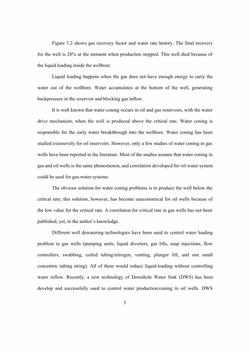
Figure 1.2 shows gas recovery factor and water rate history. The final recovery
for the well is 28% at the moment when production stopped. This well died because of
the liquid loading inside the wellbore.
Liquid loading happens when the gas does not have enough energy to carry the
water out of the wellbore. Water accumulates at the bottom of the well, generating
backpressure in the reservoir and blocking gas inflow.
It is well known that water coning occurs in oil and gas reservoirs, with the water
drive mechanism, when the well is produced above the critical rate. Water coning is
responsible for the early water breakthrough into the wellbore. Water coning has been
studied extensively for oil reservoirs. However, only a few studies of water coning in gas
wells have been reported in the literature. Most of the studies assume that water coning in
gas and oil wells is the same phenomenon, and correlation developed for oil-water system
could be used for gas-water systems.
The obvious solution for water coning problems is to produce the well below the
critical rate; this solution, however, has become uneconomical for oil wells because of
the low value for the critical rate. A correlation for critical rate in gas wells has not been
published, yet, to the author’s knowledge.
Different well dewatering technologies have been used to control water loading
problem in gas wells (pumping units, liquid diverters, gas lifts, soap injections, flow
controllers, swabbing, coiled tubing/nitrogen, venting, plunger lift, and one small
concentric tubing string). All of them would reduce liquid-loading without controlling
water inflow. Recently, a new technology of Downhole Water Sink (DWS) has been
develop and successfully used to control water production/coning in oil wells. DWS
3
7/23/2019 Armenta Dis
http://slidepdf.com/reader/full/armenta-dis 22/263
controls water inflow to the well, by reversing water coning with a second bottom
completion. That drains water from under the top completion.
The purpose of this research is to evaluate the performance of the DWS
technology controlling water production-problems in gas wells. Design and operation of
DWS gas wells is also addressed. Moreover, Identification of unique mechanisms
improving water production in gas reservoirs, and completion length optimization for
conventional gas wells are also approached.
1.2 Statement of Research Problem
In response to economic and environmental concerns, in-situ injection of water in
the same gas well, without lifting the water to surface, has become a new technology
knows as Downhole Gas-Water Separation (DGWS). Similarly to all the other
technologies use to solve liquid-loading in gas wells, DGWS does not consider the well-
reservoir interaction solving water production problem, either.
Therefore, new technologies that consider both, the well and the reservoir,
component of the water problem production in gas wells are needed. These technologies,
not only have to improve gas production/recovery from the reservoir, but have to reduce
the amount of water produced at the surface, too.
In the past, water coning in gas wells has not received much attention from
researcher in the petroleum industry. The reason for that probably is the general “feeling”
that the problem is of minimal importance or even does not exist because of the high gas
mobility compared with the water mobility. Therefore, few studies have been done
addressing reservoir mechanisms increasing water coning/production in gas reservoir.
The low gas price experienced during the last decade reduced the interest in gas well
problems at the United States. This low gas price environment, however, has slowly
4

7/23/2019 Armenta Dis
http://slidepdf.com/reader/full/armenta-dis 23/263
changed since the beginning of this century due to increases in gas demand and reduction
in gas supply, pushing people trying to explain, understand and solve gas
production/recovery problems. One such attempt includes the “pilot” work conducted for
the research described herein.
1.3 Significance and Contribution of This Research
The significance of this research stems from the following six studies:
• First, the research presents analytical and numerical evidence that the water
coning is different in gas wells than in oil wells.
•
Second, this research identifies vertical permeability, aquifer size, Non-Darcy
flow effect (N-D), density of perforation, and flow behind casing as unique
mechanisms improving water coning in gas wells.
• Third, the research presents a new perspective for N-D flow in gas reservoirs,
showing that very well accepted statements in the oil and gas industry about this
phenomenon are not correct (Non Darcy flow is not important in gas wells
flowing at low rates. Non-Darcy flow coefficient applied only to the well bore
properly represents N-D flow throughout the reservoir).
• Fourth, this research presents a new procedure to identify flow behind casing
(channeling in the cemented annulus) in gas wells.
• Fifth, the optimum completion length in gas wells for the maximum net present
value is presented. Reservoir and economic parameters affecting water production
in gas reservoir are prioritized.
• Finally, the research presents an evaluation for DWS in gas reservoirs, identifying
the reservoir conditions where the technology could be successful. The best way
5
7/23/2019 Armenta Dis
http://slidepdf.com/reader/full/armenta-dis 24/263
to operate DWS in gas reservoirs, considering different completion/production
parameters, is identified, too.
1.4 Research Method and Approach
This research uses two existing commercial numerical simulators (Eclipse 100,
and IMEX) and a radial grid model to study water coning mechanisms and DWS
evaluation in gas reservoirs. Two commercial numerical simulators are used during the
study because the first simulator used for this research (Eclipse 100) does not properly
represent N-D in gas reservoirs. N-D flow is identified as an important phenomenon.
Another simulator (IMEX) is also used. Analytical models are built to support procedures
and results for different mechanisms that increase water coning in gas reservoirs. Field
data are used to confirm analytical and numerical results from the N-D flow effect
analysis. Statistical analyses are performed with the numerical simulation results from the
analysis of mechanisms affecting water coning/production in gas wells.
Because of the very nature of this first “pilot” research of DWS in gas reservoir,
several different types of approaches, studies, and evaluations are performed.
Analytical and numerical approaches are used to identify similarities and
differences between water coning in gas and oil wells (Chapter 3). The analysis is
focused on the amount of fluid produced, under the same production conditions, from the
oil-water and gas-water system, and the shape of the interface (oil-water and gas-water)
around the wellbore for both systems. One new analytical model, to investigate gas-water
and oil-water interface shape, is developed following Muskat (1982) procedure. The
results from the analytical model are compared with results from a numerical reservoir
simulator model built with similar characteristics. Another analytical model is built to
investigate the amount of fluid produced from both systems.
6

7/23/2019 Armenta Dis
http://slidepdf.com/reader/full/armenta-dis 25/263
Qualitative studies identifying mechanisms increasing water coning/productions
in gas wells are conducted using numerical and analytical models (Chapter 4). Vertical
permeability, aquifer size, Non-Darcy flow effect, perforation density, and flow behind
casing are evaluated. Analytical models are constructed to confirm the results from the
numerical reservoir simulator models. Moreover, one analytical model is developed to
enhance the capability of reservoir simulator representing the phenomena of flow behind
casing in gas wells because the reservoir simulator does not include the annulus space
between the casing and the wellbore wall in its modeling. A new procedure identifying
flow behind casing in gas wells, using water production field data, is presented.
Analytical and numerical models are used to identify and quantify the importance
of Non Darcy flow effect in low productivity gas reservoirs. The results from the models
are compared with actual field data (Chapter 5). Recommendations on the correct way of
modeling Non Darcy flow in gas reservoir using numerical reservoir simulators are
included.
Feasibility studies of DWS in gas wells are done using reservoir numerical
models (Chapter 6). The studies compare final gas recovery for conventional gas wells
and DWS gas wells. Quantitative comparison of final gas recovery between two different
technologies solving water production problems in gas wells is made, too [One
technology solves the problem in the wellbore (DGWS), and the other one solves the
problem in the reservoir (DWS)]. Modeling DWS, and DGWS wells in commercial
numerical simulator brings several challenges because of the inability of the reservoir
simulator to perform dual completed well with two-different bottom hole condition and
two different tubing performance model at the same well. Model modifications (e.g., two
7

7/23/2019 Armenta Dis
http://slidepdf.com/reader/full/armenta-dis 26/263
wells in the same location with different completion length, two tubing performance
models for the same well, etc) are made to evaluate DWS and DGWS wells performance.
Sensitivity studies of mechanisms increasing water coning/production in gas wells
are conducted using analysis of variance. Three different linear regression models,
without interaction among the factors, for ultimate cumulative gas production, net present
value and peak gas rate are built and evaluated using numerical reservoir simulation
results. One linear regression model for the discount cash flow, considering interaction
among the eight factors, is built and evaluated (Chapter 7). Horizontal permeability,
aquifer size, permeability anisotropy, initial reservoir pressure, length of completion, gas
price, water disposal cost, and discount rate are the factors considered for the analysis.
Optimization of Net Present Value with respect to completion length in gas reservoir with
bottom-water drive, using the response model from the statistical model and the direct
result from the simulator, was done, too.
Qualification of the most important operational factors affecting DWS
performance in gas reservoir is done using numerical reservoir simulator model (Chapter
8). The analysis includes length-of-top completion, length-of-bottom completion,
drained-water rate, separation between the top-and the bottom-completion, and the time
to install DWS technology. Recommendations on how to use DWS effectively in gas
reservoirs are included.
1.5 Work Program Logic
The dissertation is divided into nine chapters. The introduction chapter presents
an overview of the problem of water production in gas wells explaining the necessity for
new technologies to solve the problem. It also presents a concise statement about the lack
8

7/23/2019 Armenta Dis
http://slidepdf.com/reader/full/armenta-dis 27/263

7/23/2019 Armenta Dis
http://slidepdf.com/reader/full/armenta-dis 28/263
10
performed. The study includes a comparison between two different technologies solving
water production problems in gas wells for the same gas reservoir [one technology solves
the problem in the wellbore (DGWS), and the other one solve the problem into the
reservoir (DWS)].
Chapter eight reviews the operational parameters involved in DWS performance
in gas reservoirs giving recommendation about the way to use the technology. Chapter
nine provides conclusions from this research work, including recommendations for future
research.

7/23/2019 Armenta Dis
http://slidepdf.com/reader/full/armenta-dis 29/263
CHAPTER 2
LITERATURE REVIEW
Liquid loading or accumulation in gas wells occurs when the gas phase does not
provide adequate energy for the continuous removal of liquids from the wellbore. The
accumulation of liquid will impose an additional back pressure on the formation, which
can restrict well productivity (Ikoku, 1984). The limited gas flow velocity for upward
liquid-drop movement is the critical velocity.
2.1 Critical Velocity
Turner, Hubbard, and Dukler (1969) analyzed two physical models for removal of
gas well liquids: the liquid droplet and the liquid film models. A comparison of these two
models with field data led to the conclusion that the onset of load up could be predicted
adequately with the droplet model, but that a 20% adjustment of the equation upward was
necessary. Equation 2.1 shows Turner et al. correlation.
2/1
4/14/1 )(912.1
g
g L
t v ρ
ρ ρ σ −= ………………………………………….(2.1)
Where vt is critical velocity (ft/sec), σ is interfacial tension (dynes/cm), ρ L is
liquid-phase density (lbm/ft3), and ρ g is gas phase density (lbm/ft3).
Turner et al. equation (Eqn. 2.1) calculating gas critical velocity has gained
widespread industry acceptance because of its close agreement with field data, and it is
widely referenced in the literature (Hutlas & Granberry, 1972; Libson & Henry, 1980;
Ikoku, 1984; Beggs, 1985; Upchurch, 1987; Bizanti & Moonesas, 1989; Smith, 1990;
Elmer, 1995).
11
7/23/2019 Armenta Dis
http://slidepdf.com/reader/full/armenta-dis 30/263
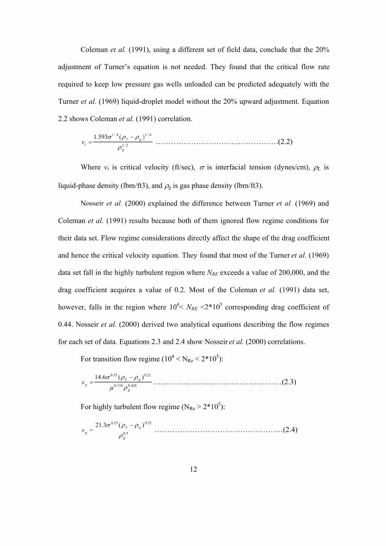
Coleman et al. (1991), using a different set of field data, conclude that the 20%
adjustment of Turner’s equation is not needed. They found that the critical flow rate
required to keep low pressure gas wells unloaded can be predicted adequately with the
Turner et al. (1969) liquid-droplet model without the 20% upward adjustment. Equation
2.2 shows Coleman et al. (1991) correlation.
2/1
4/14/1 )(593.1
g
g L
t v ρ
ρ ρ σ −= ………………………………………….(2.2)
Where vt is critical velocity (ft/sec), σ is interfacial tension (dynes/cm), ρ L is
liquid-phase density (lbm/ft3), and ρ g is gas phase density (lbm/ft3).
Nosseir et al. (2000) explained the difference between Turner et al. (1969) and
Coleman et al. (1991) results because both of them ignored flow regime conditions for
their data set. Flow regime considerations directly affect the shape of the drag coefficient
and hence the critical velocity equation. They found that most of the Turner et al. (1969)
data set fall in the highly turbulent region where N RE exceeds a value of 200,000, and the
drag coefficient acquires a value of 0.2. Most of the Coleman et al. (1991) data set,
however, falls in the region where 104< N RE <2*105 corresponding drag coefficient of
0.44. Nosseir et al. (2000) derived two analytical equations describing the flow regimes
for each set of data. Equations 2.3 and 2.4 show Nosseir et al. (2000) correlations.
For transition flow regime (104 < NRe < 2*105):
426.0134.0
21.035.0 )(6.14
g
g L
g v ρ µ
ρ ρ σ −
= ……………………………………………(2.3)
For highly turbulent flow regime (NRe > 2*105):
5.0
25.025.0 )(3.21
g
g L
g v ρ
ρ ρ σ −= ……………………………………………(2.4)
12

7/23/2019 Armenta Dis
http://slidepdf.com/reader/full/armenta-dis 31/263
Where v g is gas critical velocity (ft/sec), σ is interfacial tension (dynes/cm), ρ L is
liquid-phase density (lbm/ft3), µ is gas viscosity (lbm/ft/sec), and ρ g is gas phase density
(lbm/ft3).
Sutton et al. (2003) evaluates gas well performance at Subcritical rates. They
evaluated six different models describing the presence of a static liquid column in the
wellbore with field data from 15 wells. They concluded that the model proposed by
Hasan and Kabir (1985) offers the best approach for simulating this phenomenon.
2.2 Critical Rate for Water Coning
Water coning happens on the vicinity of the well when water moves up from the
free water level in a vertical direction. Production from a well causes a pressure sink at
the completion. If the wellbore pressure is higher than the gravitational forces resulting
from the density difference between gas and water, then water coning occurs. Equation
2.5 shows the basic correlation between pressure in the wellbore and at the well vicinity
for coning.
w g g wwell h p p −−=− )(433.0 γ γ ………………………………………………(2.5)
Where p is average reservoir pressure (psi), pwell is the flowing bottom hole
pressure (psi), γ w is water specific gravity, γ g is gas specific gravity, and h g-w is the
vertical distance from the bottom of the well’s completion to the gas/water contact (ft).
Critical rate is defined as the maximum rate at which oil/gas is produced without
production of water (Joshi, 1991). The critical rate for oil-water systems has been
discussed for several authors developing different correlations to calculate that rate. For
gas-water system, however, no correlation has been published calculating critical rate,
yet. One possible reason for the low interest in critical rate for gas-water system could be
the general “feeling” that water coning in gas wells is less important than in oil wells.
13

7/23/2019 Armenta Dis
http://slidepdf.com/reader/full/armenta-dis 32/263
Muskat (1982), for example, discussing about water coning problem said: “water coning
will be much more readily suppressed and will involve less serious difficulties for wells
producing from gas zones than for wells producing oil…the critical-pressure differential
for water coning will be probably grater by a factor of at least four in gas wells than in oil
wells.” Joshy (1991) presets an excellent discussion about critical rate in oil wells. He
included analytical and empirical correlation to calculate critical rate. The correlations
include: Craft and Hawking method (1959), Meyer, and Garder method (1954), Chaperon
method (1986), Schols method (1972), and Hoyland, Papatzacos and Skjaeveland method
(1986). Joshy presents equations and example calculation for each method, concluding
that the critical rate calculated for each method is different. He said that there is no right
or wrong critical correlation, and each one should make decision about which correlation
could be used for specific field applications. Meyer, and Garder correlation (1954), and
Schols correlation (1972) are shown here as examples of critical rate equations for oil-
water system (Eqns. 2.6 and 2.7).
Meyer and Garder correlation (1954):
)/ln(
)()(001535.0 22
weoo
ow
cr r B
Dhk q
µ
ρ ρ −−= ……………………………………………(2.6)
Where: qc is critical oil rate (STB/D), ρ w is water density (gm/cc), ρ o is oil density
(gm/cc), k is formation permeability (md), h is oil zone thickness (ft), D is completion
interval thickness (ft), µ o is oil viscosity (cp), Bo is oil formation volume factor
(bbl/STB), r e is external drainage radius (ft), and r w is wellbore radius (ft).
Schols correlation (1972):
14.022
)/ln(432.0*
2049
)()(
+
−−=
eweoo
poow
or
h
r r B
hhk q
π
µ
ρ ρ ……………………………(2.7)
14
7/23/2019 Armenta Dis
http://slidepdf.com/reader/full/armenta-dis 33/263
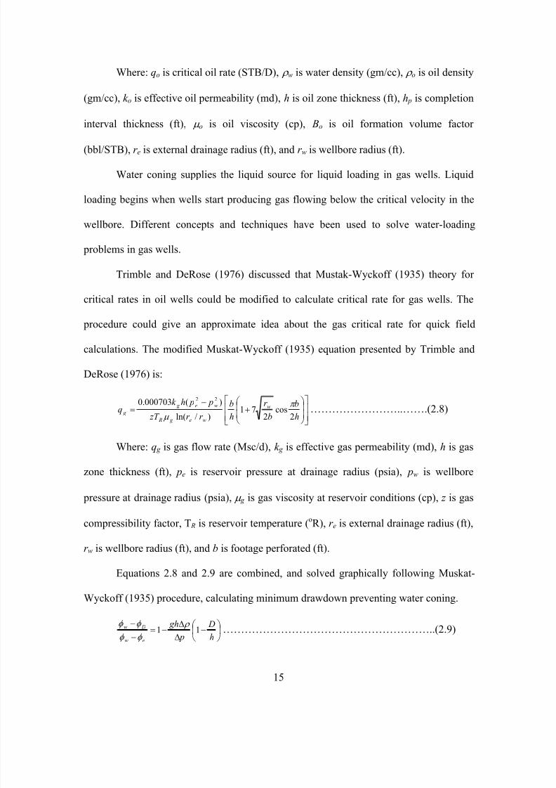
Where: qo is critical oil rate (STB/D), ρ w is water density (gm/cc), ρ o is oil density
(gm/cc), k o is effective oil permeability (md), h is oil zone thickness (ft), h p is completion
interval thickness (ft), µ o is oil viscosity (cp), Bo is oil formation volume factor
(bbl/STB), r e is external drainage radius (ft), and r w is wellbore radius (ft).
Water coning supplies the liquid source for liquid loading in gas wells. Liquid
loading begins when wells start producing gas flowing below the critical velocity in the
wellbore. Different concepts and techniques have been used to solve water-loading
problems in gas wells.
Trimble and DeRose (1976) discussed that Mustak-Wyckoff (1935) theory for
critical rates in oil wells could be modified to calculate critical rate for gas wells. The
procedure could give an approximate idea about the gas critical rate for quick field
calculations. The modified Muskat-Wyckoff (1935) equation presented by Trimble and
DeRose (1976) is:
+
−
= h
b
b
r
h
b
r r zT
p phk
q
w
we g R
we g
g 2cos271)/ln(
)(000703.0 22π
µ ……………………..…….(2.8)
Where: q g is gas flow rate (Msc/d), k g is effective gas permeability (md), h is gas
zone thickness (ft), pe is reservoir pressure at drainage radius (psia), pw is wellbore
pressure at drainage radius (psia), µ g is gas viscosity at reservoir conditions (cp), z is gas
compressibility factor, T R is reservoir temperature (oR), r e is external drainage radius (ft),
r w is wellbore radius (ft), and b is footage perforated (ft).
Equations 2.8 and 2.9 are combined, and solved graphically following Muskat-
Wyckoff (1935) procedure, calculating minimum drawdown preventing water coning.
−
∆
∆−=
−
−
h
D
p
gh
ew
Dw 11 ρ
φ φ
φ φ …………………………………………………..(2.9)
15

7/23/2019 Armenta Dis
http://slidepdf.com/reader/full/armenta-dis 34/263
Where: φ w is potential at well radius (psi), φ D is potential at well radius and depth
D (psi), φ e is potential at drainage radius (psi), g ∆ρ is difference in hydrostatic gradient at
reservoir conditions between the gas and water (psi/ft), ∆ p is pressure drawdown (psia), h
is gas zone thickness (ft), and D is distance from formation to cone surface at r (ft).
Trimble and DeRose (1976) procedure combined gas flow equation (Eqn. 2.8)
with oil graphical solution for Eqn 2.9. Changes in oil density and viscosity with respect
to pressure are negligible. Gas properties (density, and viscosity), however, strongly
depend on pressure; therefore, the previous procedure should be used as a reference with
limitations.
2.3 Techniques Used in Solving Water Loading
Techniques used in solving water loading in gas wells could be classified as:
• Tubing lift improvement:
- Chemical injection
- Physical modification
- Thermal
- Mechanical
• Bottom liquid removal:
- Mechanical
2.3.1 Tubing Lift Improvement
2.3.1.1 Chemical Injection
Chemicals are injected in gas wells with liquid loading problems to prolong the
extracting period and enhance wells’ productivity. Foam agents are used to carry the
water out of the well. The objective of using foaming agents is to create a molecular bond
between the gas and the liquid phases and to maintain its foam stability for a useful
16

7/23/2019 Armenta Dis
http://slidepdf.com/reader/full/armenta-dis 35/263
period of time so that the accumulated liquid is transported to the surface in a foamed,
slurry state (Neves & Brimhall, 1989).
Chemical composition, concentration, temperature, water salinity, presence of
condensate oil, and hydrogen sulfide are factors controlling foaming agent performance
(Xu & Yang, 1995).
Foam lift uses reservoir energy to carry out the water, reducing the critical
velocity. The most common application of foam lift is in the form of a “soap stick.” The
soap bar (1-inch diameter, 1-foot long) is dropped inside the tubing and foam is generated
by fluid mixing and agitation with the surfactant dissolved from the soap bar (Saleh, and
Al-Jamae’y, 1997).
Surfactant concentrations are difficult to gauge and control when the surfactant is
dumped into the annulus or the tubing (Lea, and Tighe, 1983).
Other applications include injection of surfactant through the annulus from the
wellhead, or downhole injection using a capillary string inside the tubing.
Libson and Henry (1980) reported successful results injecting foaming agent into
the casing annulus in very low permeability gas wells located in the Intermediate Shelf
area of Southwest Texas. After 10 days of injecting a foaming agent to the wellhead, the
gas rate increased from 142 Mscfd to 664 Mscfd, and water rate increased from 0.8 bwpd
to 3.2 bwpd.
Placing a capillary string through the producing tubing foam is injected downhole
in front of the perforations. Vosika (1983) reported foam injection an economic success
in four wells at the Great Green River Basing, Wyoming. Average gas rates increase
more than doubled when the foam agent was injected in conjunction with the methanol
used to solve traditional freezing problems.
17

7/23/2019 Armenta Dis
http://slidepdf.com/reader/full/armenta-dis 36/263
Silverman et al. (1997), and Awadzi et al. (1999) reported liquid loading success
in gas wells located in the Cotton Valley formation in East Texas using the capillary
technique. Gas rate increments in four wells went from 28.2% to 676.3%.
Surfactant injection could increase corrosion. Campbell et al. (2001) reported a
chemical mixture between the foaming agent and corrosion inhibitor to improve liquid
lifting without increasing corrosion in the wellbore.
2.3.1.2 Physical Modification
Physical modification of the wellbore has been done to increase gas velocity. Gas
velocity is increased, reducing the gas-flow area to improve gas carry capacity. A small
concentric tubing string and tubing collar insert have been proposed to improve gas
velocity. These methods of producing marginal gas wells are also viewed as a temporary
solution to liquid loading. As time elapses and the reservoir pressure declines, the smaller
diameter tubing string eventually loads up with liquids. At this point, another method
must be employed to help combat the accumulation of liquid in the wellbore (Neves &
Brimhall, 1989).
Hutlas and Grandberry (1972) reported success using a 1-in tubing string in
northwestern Oklahoma and the Texas Panhandle. Running a 1-in tubing string inside the
production tubing increased gas rate more than 100% in four wells.
Libson and Henry (1980) reported that gas rate increased by 50 Mscfd per
installation in the Intermediate Shelf area of southwest Texas when a 1.90-in tubing was
installed in a 2 3/8-in production tubing.
One-in tubing string run inside 2 7/8-in production tubing increased gas rate,
decreasing field annual decline, in seven wells, two sour gas fields, at the Edward Reef in
Texas (Weeks, 1982).
18

7/23/2019 Armenta Dis
http://slidepdf.com/reader/full/armenta-dis 37/263
Yamamoto & Christiansen (1999) and Putra & Christiansen (2001) reported
laboratory data for tubing collar inserts increasing liquid lifting. The tubing collar inserts
are restrictions installed inside the tubing string. The restrictions alter flow mechanisms
and liquid could be lifted by gas flowing below the critical velocity; the effect could be
reduced due to the pressure drop across the restriction (Yamamoto and Christiansen,
1999). Parameters affecting the tubing collars inserts include: insert geometric shape, size
and spacing of the inserts, gas and liquid flow rates, and pressure drop across the insert
(Putra and Christiansen, 2001).
Installing concentric coiled tubing is another technique used to increase gas
velocity. An estimated 15,000 wells have coiled tubing installed in them as velocity or
siphon strings. The coiled string consists of either steel or plastic tubing (Scott and
Hoffman, 1999).
Adams and Marsili (1992) presented the design and installation for a 20,500-ft
coiled tubing velocity string in the Gomez Field, Pecos County, Texas. One 1 ¼-in coiled
tubing string was installed in a 4 ½-in production tubing, solving liquid loading problems
and increasing gas production more than two-fold.
Elmer (1995) discussed the combined application of small tubing string with
some extra gas production through the casing/tubing annulus. The small tubing string
always flowed above the critical velocity, and some gas, due to extra reservoir production
capacity, was produced up to the annulus. Gas production increased 33% in two wells
and 91% in another well when this production strategy was used.
2.3.1.3 Thermal
Pigott et al. (2002) presented the first successful application of wellbore heating
to prevent fluid condensation and eliminate liquid loading in low-pressure, low-
19
7/23/2019 Armenta Dis
http://slidepdf.com/reader/full/armenta-dis 38/263
productivity gas wells. The application was in the Carthage Field. A heater cable installed
around the tubing string increased wellbore temperature, avoiding liquid condensation.
The heating technique alone increased gas production more than 100%. However,
combination of the heating technique with a compressor increased gas production more
than three-fold. Water-drive gas reservoirs are not good candidates to install the heating
technique because of the high amount of energy needed to increase wellbore temperature.
Gas wells with low liquid ratio (1 to 8 bbls/MMcf) and liquid loading problems due to
condensations are good candidates to apply the heater technique. Currently the major
limitation to widespread application of this technique is the comparatively high operating
cost. The average cost to operate the well is $5,000/month. This compares to an average
operating cost of $1,200/month in offset wells (Pigott et al., 2002).
2.3.1.4 Mechanical
Gas lift has been used to improve tubing lifting capacity. Gas lift systems inject
high-pressure gas from the casing tubing annulus through valves into liquids in the tubing
to reduce their density and move them to the surface (Lea, Winkler, and Snyder, 2003).
Gas lift may be used to removed water continuously or intermittently. Gas lift
could be used in conjunction with plunger lift and surface liquid diverters to improve its
overall efficiency (Neves & Brimhall; 1989). Gas lift could be combined with a small
concentric string (siphon string), too (Lea, & Tigher; 1983).
The main disadvantage of the gas lift method solving liquid loading is that it
would not operate efficiently to the abandonment pressure of the well. The optimum
operational efficiency is obtained when the water-lift ratio is in the range from 1.5 to 3
Mscf/bbl of water lifted. The efficiency of the gas lift technique declines in low-
20

7/23/2019 Armenta Dis
http://slidepdf.com/reader/full/armenta-dis 39/263
productivity gas wells producing in excess of 8 bwpd due to the large amount of gas
needed (Melton & Cook, 1964).
Hutlas & Granberry (1972) presented four gas wells where gas rate was increased
from 50% to more than 100% when a combined gas lift liquid-diverter system was
installed to solve liquid loading problems. The wells were located in north-western
Oklahoma and the Texas Panhandle in high-pressure fields at depths ranging from 5,100
to 8,600 ft.
Stephenson et al. (2000) presented successful installation of gas lift for
dewatering gas wells at the Box Church Field – a high water-cut gas reservoir located in
Texas. Soap sticks, swabbing, and coiled tubing/nitrogen had been used at the field try to
solve liquid loading, but these techniques provided only a short-term solution to the
problem. A 50% increase in the average gas rate of the field was reported after the
combined mechanism of gas-lift with compressor was installed in four high water-cut
(more than 200 bbl/MMscf) wells.
Gas lift had been used for dewatering gas wells down-dip increasing and
accelerating gas recovery in wells located up-dip in the same reservoir (Girardi et al ,
2001; Aguilera et al 2002) using a co-production strategy (Arcaro & Bassiouni, 1987).
Some field tests have been done to use Coproduction of gas and water as a
secondary gas recovery technique for abandoned water-out wells with limited success
(Rogers, 1984; Randolph et al , 1991).
2.3.2 Bottom Liquid Removal
Pumps, plunger, swabbing, and gas injection using coiled tubing have been used
to remove liquid from the bottom of the well after the gas is flowing below the critical
rate.
21

7/23/2019 Armenta Dis
http://slidepdf.com/reader/full/armenta-dis 40/263
2.3.2.1 Pumps
Pumping systems used to solve liquid loading in gas wells include: beam
pumping, progressive-cavity pumping, and jet pumping. The main advantage of pumping
is that they do not depend on the reservoir energy or on the gas velocity for liquid lifting
(Hutlas & Granberry, 1972).
Down-hole pumps do have application in gas wells producing high liquid rate-
over 30 bwdp (Lea & Tigher, 1983).
Beam pumping comprises a motor-driven surface system lifting sucker rods
within the tubing string to operate a downhole-reciprocating pump. The liquid is pumped
up the tubing and the gas is produced out the annulus (Libson & Henry, 1980).
Melton & Cook (1964) reported that beam units were the most efficient as well as
economical method of solving liquid loading problems in low-pressure shallow gas wells
producing between 12 and 15 bwpd on the Panhandle in the Hugton and Greenwood
fields.
Hutlas & Granberry (1972) presented a successful installation of beam units at the
Hugoton field, Kansas solving water-loading problems in gas wells. Gas rate increased
from 50% to more than 100% in four wells after the beam unit was installed.
Libson & Henry (1980) explained that production increased when beam units
were installed in low-gas rate wells (less than 40 Mscf/d) with liquid production between
10 to 40 bwpd at the intermediate Shelf area of southwest Texas, in Sutton County.
Henderson (1984) described the technical challenge of installing a beam pump
unit to solve liquid loading problems at 16,850 ft in the Pyote Gas Unit 14-1 well at the
Block 16 (Ellengurger) field located in Ward Co., Texas. The pump removed 70 bfpd,
increasing gas production at the well from 20 to 450 Mscfd.
22

7/23/2019 Armenta Dis
http://slidepdf.com/reader/full/armenta-dis 41/263
Progressing-cavity pumping systems are based on a surface-driven rotating a rod
string which, in turn, drives a downhole rotor operating within an elastomeric stator (Lea,
Winkler & Snyder; 2003). Progressive Cavity pumps have been used extensively in the
United States for the dewatering of methane coaled-bed wells (Mills & Gaymard, 1996).
There are nearly one thousand methane pumps operating in coal basins across the
United States (predominately in the Black Warrior, Appalachian, San Juan and Raton
Basins) because of the pumps’ ability to adjust from high water rate, often encounter
during initial production, as well as low water rates experienced as the coal seams begin
to water out. Progressive Cavity pumps can lift water with high contents of coal fines,
sand particles, and some gaseous fluid (Klein, 1991).
Hebert (1989) discussed the technical limitation of rod pumps in dewatering coal-
bed wells.
A current jet pump system utilizes concentric tubing string for power fluid and
produced fluid in an open power fluid system. The gas is produced from the casing
annulus. The system allows near complete drawdown since the jet suction pressure is
claimed to be capable of being reduced to near the water vapor pressure at depth that is
usually lower than the casing sales pressure (Lea & Tighe, 1983).
2.3.2.2 Swabbing
Swabbing fluids from a well consists of lowering a swabbing tool down the
tubing and physically lifting the fluids to the surface. The objective is merely to lift the
liquids from the wellbore until the reservoir energy is able to overcome the remaining
hydrostatic head and flow on its own. Swabbing is a very costly procedure that must be
repeated every time the well loads up and with more frequency as the bottomhole
pressure declines. For this reason, swabbing is viewed as only a temporary solution to
23

7/23/2019 Armenta Dis
http://slidepdf.com/reader/full/armenta-dis 42/263

7/23/2019 Armenta Dis
http://slidepdf.com/reader/full/armenta-dis 43/263
application charts are still used in the industry as feasibility criteria to select well
applying plunger lift.
Ferguson and Beauregard (1985) include some practical guidelines to the
selection of plunger lift.
Some static models for plunger lift installations have been proposed and are
widely accepted for design due to their simplicity (Wiggins et al , 1999).
Foss & Gaul (1965) made a force balance on the plunger to determine minimum
casinghead pressure to drive a liquid slug up to the surface. They also worked out the
volume of gas required in each cycle, and the minimum amount of time per cycle based
on estimates for plunger rise and fall velocities. They used an 85 well data set for some
parameters of the model.
Hacksma (1972) used the Foss & Gaul (1965) model to show how to calculate the
minimum gas-liquid ratio required for operation and the optimum gas-liquid ratio that
yields maximum production.
Abercrombie (1980) reworked the Foss & Gaul (1965) model, considering a
smaller plunger fall velocity in the gas.
Dynamic models have also been published to describe the phenomena of a
plunger life cycle. Each dynamic model made different assumptions, and different
experimental and field data were used to prove the validity of each one.
Lea (1982) presented a dynamic model that predicts, at each step, casinghead
pressure, plunger position, and plunger velocity until the slug surfaces. The results
indicated lower operating pressure and lower gas requirement than the static models.
25
7/23/2019 Armenta Dis
http://slidepdf.com/reader/full/armenta-dis 44/263
White (1982) experimentally evaluated liquid fallback in a reduced scale
apparatus. He concluded that 10% of the initial liquid column fallback for each plunger
run. He included some recommendations to design a hybrid plunger-gas lift system.
Rosina (1983) developed a dynamic model similar to that of Lea (1982), but
taking into account liquid fallback. He also conducted experiments to verify the
prediction of his model.
Mower et al. (1985) conducted a laboratory investigation on gas slippage and
liquid fallback for commercial plungers. They proposed a modified Foss & Gaul (1965)
model incorporating these effects. The model was then adjusted to fit field data from four
wells.
Avery and Evans (1988) proposed a dynamic model for the entire plunger cycle,
incorporating the reservoir performance. They assumed that each cycle started as soon as
the plunger arrived at the bottom.
Marcano and Chacin (1992) presented another dynamic model for the full cycle.
Liquid fallback through plunger was considered according to Mower et al.’s (1985)
empirical data.
Hernandez et al. (1993) conducted experiments to evaluate liquid fallback and
plunger rise velocity.
Gasbarri and Wiggins presented a dynamic model including a reservoir model.
Their model incorporated frictional effect of the liquid slug and the expanding gas above
and below the plunger and considered separator and flowline effect.
Maggard et al. (2000) developed another dynamic model considering a transient
reservoir performance. They concluded that assuming a stabilized reservoir model is a
conservative assumption for plunger lift behavior.
26

7/23/2019 Armenta Dis
http://slidepdf.com/reader/full/armenta-dis 45/263
Optimization of plunger has been presented based on experimental and simulator
studies. Baruzzi & Alhanti (1995) recommend no perfect seal plunger during buildup
because it obstructs the passage of liquid and gas above the plunger.
Wiggins et al. (1999) suggested that optimum production rates would be achieved
by allowing the well to produce as long as possible prior to shut in. Excessive gas
production periods, however, run the risk of killing the well by building a liquid slug that
is too long to be lifted by the remaining energy stored in the annulus.
Schwall (1989) reported gas production increases of 50 to 100% after plunger lift
installation on gas wells with gas-liquid ratio ranges from 3 Mscf/bbl to 20 Mscf/bbl, and
gas rate between 15 Mscfd and 54 Mscfd located in the South Burns Chapel Field in
northern West Virginia.
Brady & Morrow (1994) evaluated the performance of plunger lift for 130 low-
pressure, tight-sand gas wells located in Ochiltree County, Texas. They concluded that
the total daily production rate increase attributed to the plunger lift was nearly 70 Mscfd
per well, and an incremental 32 Bcf of gross gas reserves are directly attributable to
plunger lift installation.
Schneider and Mackey (2000) presented results in which initial gas production
increased 85% after the wells located in the Eumont gas play at New Mexico were
converted to plunger lift from beam pumps.
2.3.2.4 Downhole Gas Water Separation
Downhole Gas Water Separation (DGWS) are devices that separate gas from
water at the bottom of gas wells. The separated water is reinjected into a non-productive
interval, while the gas is produced to the surface (Rudlop & Miller, 2001).
27

7/23/2019 Armenta Dis
http://slidepdf.com/reader/full/armenta-dis 46/263
Nichols & Marsh (1997) explained that several available commercial
configurations or devices have been reported to be suitable for re-injecting water into a
lower zone within a gas producing well:
• A conventional insert pump with a “bypass” sub
• A specially designed insert pump with displaces on the downstroke
• Progressive cavity pumps
• Electrical submersible pumps
Grubb and Duval (1992) presented a new water disposal tool called a “Seating
Nipple Bypass.” The bypass tool allows liquid to be lifted up the tubing in the usual way;
however, small drain holes permit the liquid to bypass down past the pump to a point in
the tubing string below the pump intake. A packer provides hydraulic isolation between
production and injection intervals. When the liquid head is sufficiently high, it will then
flow into the disposal zone. The bypass tool was tested in seven well in the Oklahoma
Panhandle and Southwest Kansas, some of which were temporarily abandoned before the
installation. A conventional beam-pumping unit lifted the water. The tool proved
successful in five wells. One well produced 348 Mscfd without water after the installation
and 300 Mscfd and 300 bwpd before the installation.
Klein & Thompson (1992) explained the design criteria and field installation
results for a closed-loop downhole injection system used in a water flooding oil well. The
pumping system consisted of a sucker rod driven progressing cavity pump installed
below the bottom packer. Water from the water source zone entered the pump through a
perforated sub in the tubing string above the pump and was pumped into the lower
injection zone. The pump was able to inject water at its maximum rate-180 bpd- without
28

7/23/2019 Armenta Dis
http://slidepdf.com/reader/full/armenta-dis 47/263
29
any mechanical problems. They concluded that the system could be used for dewatering
gas wells.
Nichols & Marsh (1997) presented the results for the DGWS installation in a well
in central Alberta, Canada. A “bypass tool” with a conventional insert pump and gas
powered beam pumping unit was used. With the DGWS system operating, surface
production rates were 777 Mscfd gas and 195 bwpd; without the DGWS, production was
565 Mscfd gas and 440 bwpd. In this installation, wellbore diameter limited the pump
size and its flow capacity.
Rudolph and Miller (2001) reviewed 53 wells with various DGWS installations.
Gas production increased in 29 wells, decreased in 13 wells, and did not change in 11
wells. They concluded that DGWS could work in a low rate water producing gas well
with competent cement sheath, low pressure, and a high-injectivity disposal zone below
the producing interval.
Water rate at the surface was successfully cut from 32 bbls/d to zero while gas production
increased from 300 Mscfd to 400 Mscfd when a DGWS system (Reverse flow injection
pump) was installed in a well at Hugoton Field, Oklahoma (E&P Environment, 2001).

7/23/2019 Armenta Dis
http://slidepdf.com/reader/full/armenta-dis 48/263
CHAPTER 3
MECHANISTIC COMPARISON OF WATER CONING IN OIL AND GAS
WELLS
Water coning in gas wells has been understood as a phenomenon similar to that in
oil well. In contrast to oil wells, relatively few studies have been reported on aspects of
water coning in gas wells.
Muskat (1982) believed that the physical mechanism of water coning in gas wells
is identical to that for oil wells; moreover, he said that water coning would cause less
serious difficulties for wells producing from gas zones than for wells producing oil.
Trimble and DeRose (1976) supported Muskat’s theory with water coning data
and simulation for Todhunters Lake Gas field. They calculated water-free production
rates using the Muskat-Wyckof (1935) model for oil wells in conjunction with the graph
presented by Arthurs (1944) for coning in homogeneous oil sand. The results were
compared with a field study with a commercial numerical simulator showing that the
rates calculated with the Muskat-Wyckof theory were 0.7 to 0.8 those of the coning
numerical model for a 1-year period.
The objective of this study is to compare water coning in gas-water and oil-water
systems. Analytical and numerical models are used to identify possible differences and
similarities between both systems.
3.1 Vertical Equilibrium
A hydrocarbon-water system is in vertical equilibrium when the pressure
drawdown around the wellbore is smaller than the pressure gradient generated by the
density contrast between the hydrocarbon and water at the hydrocarbon-water interface.
Equation 3.1 shows the pressure gradient for gas-water system.
30

7/23/2019 Armenta Dis
http://slidepdf.com/reader/full/armenta-dis 49/263
w g g w h p −−=∆ )(433.0 γ γ ………………………………………………(3.1)
Where ∆ p is pressure gradient (psia), γ w is water specific gravity, γ g is gas specific
gravity, and h g-w is the vertical distance from the reference level to the gas-water
interface, normally from the bottom of the well’s completion to the gas/water contact (ft).
Vertical equilibrium concept is the base for critical rates calculations. Critical
rate, in gas-water systems, is defined as the maximum rate at which gas wells are
produced without production of water.
3.2 Analytical Comparison of Water Coning in Oil and Gas Wells before Water
Breakthrough
Two hydrocarbon systems, oil and gas, in vertical equilibrium with bottom water
are considered to compare water coning in oil and gas wells before breakthrough. The
two systems have the same reservoir properties and thickness, and are perforated at the
top of the producing zone.
well
re= 1000 ft
µw=0.56 cp
w= 1.02 r/cc
rw= 0.5 ft
50 ft
20 ft
Oil Gas
µ= 1.0 cp 0.017 cp
ρ= 0.8 r/cc 0.1 r/cc
water
K= 100 md
φ=0.2
P=2000 psiT= 112 oF
Figure 3.1 Theoretical model used to compare analytically water coning in oil andgas wells before breakthrough.
31

7/23/2019 Armenta Dis
http://slidepdf.com/reader/full/armenta-dis 50/263
Figure 3.1 shows a sketch of the reservoir system including the properties and
dimensions. The mathematical calculations are included in Appendix A.
A pressure drawdown needed to generate the same static water cone below the
penetrations, and the fluid rate for each system was calculated. For the system of oil and
water and a cone height of 20 ft, a pressure drawdown equal to 2 psi is needed, and the
oil production rate is 6.7 stb/d. In the case of a gas-water system, for the same 20 ft
height of water cone 8 psi pressure drop is needed, and the gas production rate of 1.25
MMscfd.
From this first simple analysis it is evident that it is possible to have a stable water cone
of any given height in the two systems (oil-water and gas-water). For the same cone
height in vertical equilibrium, pressure drop in the gas-water system is four times greater
than the pressure drop in the oil-water system. There is a big difference in the fluids
production rate for gas-water and oil-water system. On the basis of British Thermal Units
(BTU), the energy content of one Mscf of natural gas is about 1/6 of the energy content
of one barrel of oil (Economides, 2001). For this example, the 1.25 MMscf are equivalent
to the BTU content of 208 barrels of oil. Therefore, for the same water cone height, it
would be economically possible to produce gas-water systems at the gas rate below
critical. However, in most cases it would not be not economically possible to produce oil-
water systems without water breakthrough.
3.3 Analytical Comparison of Water Coning in Oil and Gas Wells after Water
Breakthrough
The objective is to compare the shape of oil-water and gas-water interfaces at the
wellbore after water breakthrough. After the water breakthrough, there is a stratified
inflow of oil or gas with the water covering the bottom section of the well completion.
Again, two systems having the same reservoir properties and thickness are compared (oil-
32

7/23/2019 Armenta Dis
http://slidepdf.com/reader/full/armenta-dis 51/263
water and gas-water). Both systems are totally penetrated. An equation describing
interface shape was derived using the assumptions of Muskat (1982). Figure 2 shows a
sketch of the theoretical model, and Appendix A gives the derivation and mathematical
computations.
In reality the resulting equations will not describe perfectly the inflow at the well.
However, they are useful to compare the coning phenomenon in oil-water and gas-water
systems.
well
r
Pw
r
=?e
hoil / gas
water
Pe
Figure 3.2 Theoretical model used to compare analytically water coning in oil and
gas wells after breakthrough.
The resulting equations for the water coning analysis are:
For the oil-water system the interface height is described as,
+=
1
b
a
h y …………………………………………………………………(3.1)
here a, and b are constants described as,kh
Qa oo
πφ
µ
2=
kh
Qb ww
πφ
µ
2= .
e
e
y
yh
b
a −= …….………………………………………………………………(3.2)
33

7/23/2019 Armenta Dis
http://slidepdf.com/reader/full/armenta-dis 52/263
For the gas-water system the interface height is represented as,
[ ] pba
hp y
+=
)/(………………………………………………………………(3.3)
here a, b, and p are calculated using:kh
Qa
g g
πφ 2= ,
kh
Qb ww
πφ
µ
2= , and
e
e
e ph y
h y
b
a*
)/(
)]/(1[ −= ………………………………………………………………(3.4)
+
+−−=
ba p
ba p
b
a p p
br
r e
e
e
/
/ln
1ln ………………………………………….(3.5)
From Equation 3.1 it becomes obvious that when the well’s inflow of oil and water
is stratified so the upper and bottom sections of completion produce oil and water
respectively, under steady state flow conditions the interface between the two fluids is
constant and perpendicular to the wellbore because the parameter describing the interface
height are all constant and depends on the system geometry.
For the gas-water system, nevertheless, the interface height depends on the
geometry of the system, and the pressure distribution in the reservoir (Equation 3.3).
In order to demonstrate the model for gas-water systems describing the interface
between gas-water, one example was solved.
The system data are as follow: pe = 2000 psi r e = 2000 ft r w = 0.4 ft
h = 50 ft ye = 40 ft µ w = 0.498 cp Bw = 1.0
k = 100 md φ = 0.25 µ g = 0.017 cp
The procedure is as follows:
1. Assuming a value for the pressure drawdown (300 psi).
2. Calculating the flowing bottom hole pressure ( )17003002000 =−=∆−= p p p ew ,
assuming that pw is constant along the wellbore.
34

7/23/2019 Armenta Dis
http://slidepdf.com/reader/full/armenta-dis 53/263
3. Computing the water flow rate (Qw) using Darcy’s law equation (Kraft and
Hawkins, 1991):
2000
)4.0/2000ln(*0.1*498.0
)17002000(*40*100*00708.0
)/ln(
)(00708.0=
−=
−=
weww
weww
r r B
p pkhQ
µ
4. Calculating a/b, using EquationA-16 in Appendix A:
[ ]500
)50/40(
2000*)50/40(1
)/(
)/(1=
−=
−= e
e
e ph y
h y
b
a, which is constant for the system
and independent for the gas rate.
5. Finding Q g , from Equation A-15 in Appendix A:
ww
g g
Q
Q
b
a
µ = ⇒
498.0*2000
615.5*017.0*500
g Q= Q g = 5.22 MMscf/d
Note that WGR is constant for the system and depends only on the system geometry
( ye , h) and pressure drive ( pe).
6. Computing 1/b, using Equation A-17 in Appendix A:
+
+
−−
=
)/(
)/(ln)(
ln1
ba p
ba p
b
a p p
r
r
b
w
ewe
w
e
( )031.0
5001700
5002000ln500)17002000(
4
6000ln
1=
++
−−
=b
7. Assuming pressure values between pe and pw, radii r and the gas-water profile y are
calculated, using Equations A-14 and A-18 respectively in Appendix A. This is the
gas-water interface profile. The equation used to calculate pressure distribution in
the reservoir is:
35
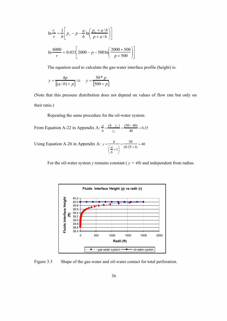
7/23/2019 Armenta Dis
http://slidepdf.com/reader/full/armenta-dis 54/263
+
+−−=
ba p
ba p
b
a p p
br
r ee
e
/
/ln
1ln
+
+−−=
500
5002000ln5002000031.0
6000ln
p
p
r
The equation used to calculate the gas-water interface profile (height) is:
[ ] pba
hp y
+=
)/(⇒
[ ] p
p y
+=
500
*50
(Note that this pressure distribution does not depend on values of flow rate but only on
their ratio.)
Repeating the same procedure for the oil-water system:
From Equation A-22 in Appendix A: 25.040
)4050()(=
−=
−=
e
e
y
yh
b
a
Using Equation A-26 in Appendix A: 40)125.0(
50
1
=+
=
+
=
b
a
h y
For the oil-water system y remains constant ( y = 40) and independent from radius.
Fluids Interface Height (y) vs radii (r)
38.4
38.638.8
39.0
39.2
39.4
39.6
39.8
40.0
40.2
0 500 1000 1500 2000 2500
Radii (ft)
F l u i d s
I n t e r f a c e
H e i g h t
( f t )
gas-water system oil-water system
Figure 3.3 Shape of the gas-water and oil-water contact for total perforation.
36

7/23/2019 Armenta Dis
http://slidepdf.com/reader/full/armenta-dis 55/263
Figure 3.3 shows the resulting profiles of the fluid interface in gas-water and oil-
water systems. After breakthrough, the oil-water interface at the well’s completion is
horizontal, while the gas-water interface tends to cone into the water. For this example
the total length of the gas cone is 1.4 ft.
3.4 Numerical Simulation Comparison of Water Coning in Oil and Gas Wells
after Water Breakthrough
One numerical simulator model was built to confirm the previous finding about
the cone shape around the wellbore. Figure 3.4 shows the numerical model with its
properties. Table 3.1 shows fluids properties used, and Appendix B contains Eclipse data
deck for the models.
600 ft
k= 10 md SGgas= 0.6
φ=0.25 APIoil=
Pinitial=2300 psi T= 110 oF
Water (W)
Gas
or
Oil
9 layers 5 ft
thick, and one layer 550 ft
thick.
100 layers
of 0.5 ft thick
Top: 5000 ft
5000 ft
50 ft
Well, r w= 3.3 in
Figure 3.4 Numerical model used for comparison of water coning in oil-water and
gas-water systems.
37

7/23/2019 Armenta Dis
http://slidepdf.com/reader/full/armenta-dis 56/263
Table 3.1 Gas, water and oil properties used for the numerical simulator model
Gas Deviation Factor and Viscosity (Gas-water model)
Press Z Visc
100 0.989 0.0122
300 0.967 0.0124500 0.947 0.0126
700 0.927 0.0129
900 0.908 0.0133
1100 0.891 0.01371300 0.876 0.0141
1500 0.863 0.0146
1700 0.853 0.01511900 0.845 0.0157
2100 0.840 0.0163
2300 0.837 0.0167
2500 0.837 0.0177
2700 0.839 0.0184
3200 0.844 0.0202
Gas and Water Relative Permeability (Gas-water model)
Sg Krg Pc
0.00 0.000 0.0
0.10 0.000 0.00.20 0.020 0.0
0.30 0.030 0.0
0.40 0.081 0.0
0.50 0.183 0.00.60 0.325 0.0
0.70 0.900 0.0
Sw Krw Pc
0.3 0.000 0.0
0.4 0.035 0.0
0.5 0.076 0.00.6 0.126 0.0
0.7 0.193 0.0
0.8 0.288 0.0
0.9 0.422 0.0
1.0 1.000 0.0
Oil and Water Relative Permeability (Oil-water model)Sw Krw Krow Pcow
0.27 0.000 0.900 00.35 0.012 0.596 0
0.40 0.032 0.438 0
0.45 0.061 0.304 00.50 0.099 0.195 0
0.55 0.147 0.110 0
0.60 0.204 0.049 00.65 0.271 0.012 0
0.70 0.347 0.000 0
38

7/23/2019 Armenta Dis
http://slidepdf.com/reader/full/armenta-dis 57/263
Following similar procedures used for the analytical comparison, again, two
systems having the same reservoir properties and thickness are compared (oil-water and
gas-water). Both systems are totally penetrated and produced at the same water rate. The
cone shape around the wellbore is investigated. Figures 3.5 and 3.6 show the results.
Swept ZoneSwept Zone
Irreducible water
Saturation
Irreducible water
Saturation
Gas-Water Oil-Water
Figure 3.5 Numerical comparison of water coning in oil-water and gas-water systems
after 395 days of production.
Figure 3.5 depicts water saturation in the reservoir after 392 days of production
for gas-water and oil-water systems. The initial water-hydrocarbon contact was at 5050
ft. In both systems the cone is developed almost in the same shape and height.
Figure 3.6 shows a zoom view at the top of the cone for both systems. For the oil-
water system, the cone interface at the top is flat. For the gas-water system, however, the
39

7/23/2019 Armenta Dis
http://slidepdf.com/reader/full/armenta-dis 58/263
cone interface is cone-down at the top. For this model the total length of the gas cone is
1.5 ft. One can see that the numerical model represents exactly the same behavior
predicted for the analytical model used previously.
Gas-Water System Oil-Water System
Figure 3.6 Zoom view around the wellbore to watch cone shape for the numerical
model after 395 days of production.
From comparison of water coning after breakthrough in gas-water and oil-water
systems, it is possible to conclude that in gas wells, water cone is generated in the same
way as in the oil-water system. The shape at the top of the cone, however, is different in
oil-water than in gas-water systems. For the oil-water system the top of the cone is flat.
For the gas-water system a small inverse gas cone is generated locally around the
40

7/23/2019 Armenta Dis
http://slidepdf.com/reader/full/armenta-dis 59/263
completion. This inverse cone restricts water inflow to the completions. Also, the inverse
gas cone inhibits upward progress of the water cone.
3.5 Discussion About Water Coning in Oil-Water and Gas-water Systems
The physical analysis of water coning in oil-water and gas-water systems is the
same. In both systems, water coning is generated when the drawdown in the vicinity of
the well is higher then the gravitational gradient due to the density contrast between the
hydrocarbon and the water.
The density difference between gas and water is grater than the density difference
between oil and water by a factor of at least four (Muskat, 1982). Because of that, the
drawdown needed to generate coning in the gas-water system is at least four-time grater
than the one in oil-water system. Pressure distribution, however, is more concentrated
around the wellbore for gas wells that for oil wells (gas flow equations have pressure
square in them, but oil flow equations have liner pressure; inertial effect is important in
gas well, and negligible in oil wells). This property makes water coning greater in gas
wells than in oil wells.
Gas mobility is higher that water mobility. Oil mobility, however, is lower than
water mobility. This situation makes water coning more critical in oil-water system than
in gas-water systems.
Gas compressibility is higher than oil compressibility. Then, gas could expand
larger in the well vicinity than oil. Because of this expansion, gas takes over some extra
portion of the well-completion (the local reverse cone explained in the previous section)
restricting water inflow.
In short, there are factor increasing and decreasing water coning tendency in both
system. The fact that oil-water systems appear more propitious for water coning
41

7/23/2019 Armenta Dis
http://slidepdf.com/reader/full/armenta-dis 60/263
42
development should not create the appearance that the phenomena is not important is gas-
water system.

7/23/2019 Armenta Dis
http://slidepdf.com/reader/full/armenta-dis 61/263
CHAPTER 4
EFFECTS INCREASING BOTTOM WATER INFLOW TO GAS WELLS
In contrast to oil wells, relatively few studies have been reported on aspects of
mechanisms of water coning in gas wells. Kabir (1983) investigated water-coning
performance in gas wells in bottom-water drive reservoirs. He built a numerical simulator
model for a gas-water system and concluded that permeability and pay thickness are the
most important variables governing coning phenomenon. Other variables such as
penetration ratio, horizontal to vertical permeability, well spacing, producing rate, and the
impermeable shale barrier have very little influence on both the water-gas ratio response
and the ultimate recovery.
Beattle and Roberts (1996) studied water-coning behavior in naturally fractured
gas reservoirs using a simulator model. They concluded that coning is exacerbated by
large aquifer, high vertical to horizontal permeability, high production rate, and a small
vertical distance between perforations and the gas-water contact. Ultimate gas recovery,
however, was not significantly affected.
McMullan and Bassioni (2000), using a commercial numerical simulator, got
similar results to Kabir (1983) for the insensitivity of ultimate gas recovery with variation
of perforated interval and production rate. They demonstrated that a well in the bottom
water-drive gas reservoir would produce with a small water-gas ratio until nearly its
entire completion interval is surrounded by water.
The objective of this study is to identify and evaluate specific mechanisms
increasing water coning/production in gas wells. Analytical and numerical models are
43

7/23/2019 Armenta Dis
http://slidepdf.com/reader/full/armenta-dis 62/263
used to identify the mechanisms. The mechanisms investigated are vertical permeability,
aquifer size, Non-Darcy flow effect, density of perforation, and flow behind casing.
4.1 Effect of Vertical Permeability
It is postulated here, in agreement with Beattle and Roberts (1996), that high
vertical permeability should generate early water production in gas reservoirs with
bottom water-drive. Vertical permeability accelerates water coning because high vertical
permeability would reduce the time needed for a water cone to stabilize.
A numerical reservoir model, shown in Figure 4.1, was adopted to evaluate the
effect of vertical permeability in gas wells. Reservoir and fluid properties used in the
model are shown on Figure 4.1 and Table 3.1, respectively. A sample data deck for the
Eclipse reservoir model is contained in Appendix C.
Well, r w = 3.3 in
Water
Gas
30 ft
9 layers 10 ft,and one layer
110 ft thick
100 layers
1 ft thick
2500 ft
5000 ft
100 ft
φ= 25% Swir = 30%Sgr = 20% S.G.gas=0.6
Pinitial= 2300 psia k r = 10 md
200 ft
Figure 4.1 Numerical reservoir model used to investigate mechanisms improvingwater coning/production (vertical permeability and aquifer size).
Horizontal permeability is set at 10 md, and four different values of vertical
permeability, 1, 3, 5, and 7 md, were considered (Permeability anisotropy, k v/k h, equal to
44

7/23/2019 Armenta Dis
http://slidepdf.com/reader/full/armenta-dis 63/263
0.1, 0.3, 0.5, and 0.7 respectively). The wells are produced at constant tubing head
pressure of 500 psia (maximum gas rate). The completion penetrates 30% of the gas zone
at the top. The results are shown in Figures 4.2a,b,c, and d.
Figure 4.2-a k v/k h = 0.1 Figure 4.2-b k v/k h = 0.3
Figure 4.2-c k v/k h = 0.5 Figure 4.2-d k v/k h = 0.7
Figure 4.2 Distribution of water saturation after 395 days of gas production.
45

7/23/2019 Armenta Dis
http://slidepdf.com/reader/full/armenta-dis 64/263
Figure 4.2 depicts water saturation in the reservoir after 395 days of gas
productions for the four values of vertical permeability. The initial water-gas contact was
at 5100 ft. The top of the cone for k v/k h equal to 0.1, 0.3, 0.5, and 0.7 is at 5080 ft, 5038
ft, 5025 ft, and 5021 ft respectively after 760 days of production. For k v/k h equal to 0.1,
and 0.3 the water cone is still below the completion and there is no water production. In
short, Figure 4.2 shows that water coning increases with vertical permeability.
0
20
40
60
80
100
120
140
160
0 1000 2000 3000 4000 5000 6000 7000
Time (Days)
W a t e r R a t e ( s t b / d )
Kv / Kh = 0.1 Kv / Kh = 0.3 Kv / Kh = 0.5 Kv / Kh = 0.7
Figure 4.3 Water rate versus time for different values of permeability anisotropy.
Figure 4.3 shows water rate versus time for the four different values of vertical
permeability. Figure 4.3 shows that water breakthrough time and water rate increase with
permeability anisotropy. The shortest water breakthrough time and highest water rate is
for k v/k h equal to 0.7. The longest water breakthrough and lowest water rate time is for
k v/k h equal to 0.1.
46

7/23/2019 Armenta Dis
http://slidepdf.com/reader/full/armenta-dis 65/263
From this study, one can say that vertical permeability increases water
coning/production in gas wells. The higher the vertical permeability is, the higher the
water coning/production of the well.
4.2 Aquifer Size Effects
Textbook models of water inflow for material balance computations assume that
the amount of water encroachment into the reservoir is related to the aquifer size (Craft &
Hawkins, 1991). (For example, van Everdinger and Hurst used the term B’ to represent
the volume of aquifer. Fetkovich’s model considers a factor called W ei defined as the
initial encroachable water in place at the initial pressure.)
Effect of aquifer size was investigated using the same numerical model used on
the previous section. Vertical and horizontal permeability are set at 10 and 1 md
respectively (k v/k h equal to 0.1). All parameters in the model were kept constant except
for the aquifer size. V AD is defined as the ratio of the aquifer pore volume to the gas pore
volume. V AD determines the amount of reservoir energy that can be provided by water
drive. The aquifer is represented by setting porosity to 10 (a highly fictitious value for
porosity), for the outermost gridblocks and the thickness of the lowermost gridblocks are
varied from 110 to 710 ft to adjust aquifer volume. V AD is varied from 346 to 1383. A
sample data deck for the Eclipse reservoir model is included in Appendix C. The results
are shown in Figures 4.4-a,b,c, and d.
Figure 4.4 depicts water saturation in the reservoir after 1124.8 days of gas
productions for the four values of V AD. The initial water-gas contact was at 5100 ft. The
top of the cone for V AD equal to 346, 519, 864, and 1383 is at 5046 ft, 5040 ft, 5034 ft,
and 5030 ft respectively; after 760 days of production. Figure 4.4, consequently, shows
that water coning increases with the aquifer size.
47

7/23/2019 Armenta Dis
http://slidepdf.com/reader/full/armenta-dis 66/263
Figure 4.4-a VAD = 346 Figure 4.4-b VAD = 519
Figure 4.4-c VAD = 864 Figure 4.4-d VAD = 1383
Figure 4.4 Distribution of water saturation after 1124.8 days of gas production.
Figure 4.5 shows water rate versus time for the four different values of vertical
permeability. Figure 4.5 shows that water rate increase with aquifer size. Water
breakthrough time, however, is not affected by aquifer size.
48

7/23/2019 Armenta Dis
http://slidepdf.com/reader/full/armenta-dis 67/263
0
20
40
60
80
100
120
140
160
0 1000 2000 3000 4000 5000 6000
Time (Days)
W a t e r R a t e
( s t b / d )
Vad = 346 Vad = 519 Vad = 864 Vad = 1383
Figure 4.5 Water rate versus time for different values of aquifer size.
Figures 4.3 and 4.5 show that vertical permeability is more important than aquifer
size in controlling the water breakthrough time. Both aquifer size and vertical
permeability, however, play an important role in increasing water rate.
From this study, one could conclude that aquifer size increases water
coning/production in gas wells without affecting water breakthrough time. The higher the
size of the aquifer is, the higher the water coning/production of the well.
4.3 Non-Darcy Flow Effects
Non-Darcy flow generates an extra pressure drop around the well bore that could
intensify water coning. Non-Darcy flow happens at high flow velocity, which is a
characteristic of gas converging near the well perforations.
The extra pressure drop is a kinetic energy component in the Forchheimer’s
formula (Lee & Wattenbarger, 1996),
2v
dL
dp βρ =− ……………..………….………..…………………..(4.1)
49

7/23/2019 Armenta Dis
http://slidepdf.com/reader/full/armenta-dis 68/263

7/23/2019 Armenta Dis
http://slidepdf.com/reader/full/armenta-dis 69/263
Water inflow model (Beggs, H.D., 1984):
])/[ln(
)(00708.0
S r r B
P P hk q
weww
wewww +
−=
µ ……………………………………………..….(4.5)
where: …………………..……………………………(4.6) ppdpd S S S S ++=
Skin factor representing mud filtrate invasion (Jones & Watts, 1971):
)/ln(1)(
2.01 wd
d
g
per
wd
per
g
d r r k
k
h
r r
h
hS
−
−−= ………………………………...(4.7)
Skin factor representing perforation density (McLeod, 1983):
[ ]
−
=
d
g
dp
g
pdp
p p
g
dp
k
k
k
k r r
n L
hS )/ln( …….……………………………………...(4.8)
Skin factor due to partial penetration (Saidikowski, 1979):
−
−= 2ln1
V
H
w
g
per
g
ppk
k
r
h
h
hS …………………………………………….…(4.9)
Non-Darcy skin around the well (Beggs, H.D., 1984):
w g g
r g g
r
r h
k D
µ
β γ 1510*22.2 −
= ………………..……………………………..(4.10)
2.1
1010*33.2
g
r k
= β …………………….……..….……………………….(4.11)
Non-Darcy skin in the crashed rock around the perforation tunnels (McLeod, 1983):
= −
g
g g g
p p p
dp
p
hk
r Ln D
µ
γ β
22
1510*22.2 ……………………………………….…...(4.12)
dp
dpk
1010*6.2= β ……………………………………………..…………(4.13)
Figure 4.7 shows a sketch for the skin component at the well for a single perforation.
51
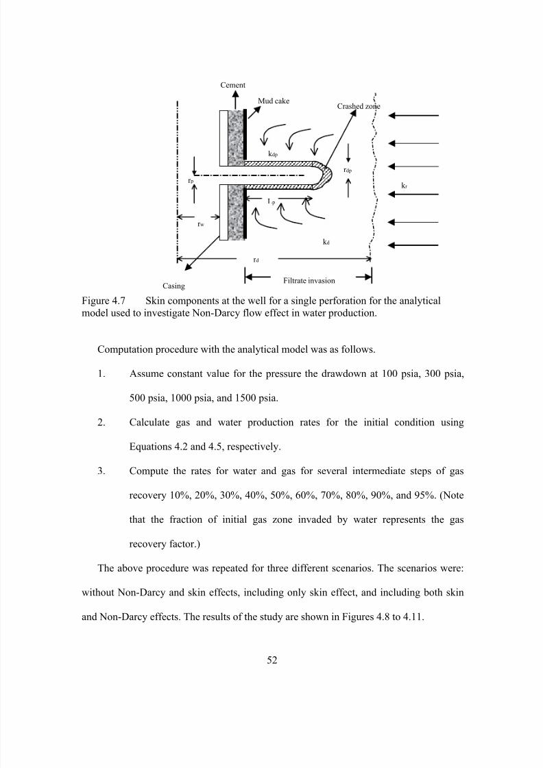
7/23/2019 Armenta Dis
http://slidepdf.com/reader/full/armenta-dis 70/263
Cement
Crashed zone
Filtrate invasionCasing
Mud cake
r dp
k d
r d
r w
k dp
k rr p
L p
Figure 4.7 Skin components at the well for a single perforation for the analytical
model used to investigate Non-Darcy flow effect in water production.
Computation procedure with the analytical model was as follows.
1. Assume constant value for the pressure the drawdown at 100 psia, 300 psia,
500 psia, 1000 psia, and 1500 psia.
2. Calculate gas and water production rates for the initial condition using
Equations 4.2 and 4.5, respectively.
3. Compute the rates for water and gas for several intermediate steps of gas
recovery 10%, 20%, 30%, 40%, 50%, 60%, 70%, 80%, 90%, and 95%. (Note
that the fraction of initial gas zone invaded by water represents the gas
recovery factor.)
The above procedure was repeated for three different scenarios. The scenarios were:
without Non-Darcy and skin effects, including only skin effect, and including both skin
and Non-Darcy effects. The results of the study are shown in Figures 4.8 to 4.11.
52

7/23/2019 Armenta Dis
http://slidepdf.com/reader/full/armenta-dis 71/263

7/23/2019 Armenta Dis
http://slidepdf.com/reader/full/armenta-dis 72/263
Figure 4.9 indicates that mechanical skin alone slightly increases WGR.
0
200
400
600
800
1,000
1,200
1,400
1,600
0 0.1 0.2 0.3 0.4 0.5 0.6 0.7 0.8 0.9 1
Recovery Factor (%)
W a t e r - G a s R a t i o ( B L S / M M S C F )
Draw-Down = 100 psi Draw-Down = 300 psi Draw-Down = 500 psi
Draw-Down = 1000 psi Draw-Down = 1500 psi
Figure 4.10 Water-Gas ratio versus gas recovery factor for total penetration of gas and
water columns, skin and Non-Darcy effect included.
Figure 4.10 indicates that combined effects of skin and Non-Darcy flow would
strongly increase water production in gas wells. Also, WGR increases with increasing
pressure drawdown.
Figure 4.11 shows WGR histories for a gas well penetrating only the gas column.
Reducing well completion to the gas column does not change WGR development; the
WGR history is similar to that of complete penetration. Interestingly, although the
completion bottom is at gas-water contact, the production is practically water-free for
almost half of the recovery. This finding is in agreement with the analytical analysis of
gas-water interface and the inverse internal cone mechanism presented in previous
sections.
54

7/23/2019 Armenta Dis
http://slidepdf.com/reader/full/armenta-dis 73/263
0
200
400
600
800
1,000
1,200
1,400
1,600
0 0.1 0.2 0.3 0.4 0.5 0.6 0.7 0.8 0.9 1
Recovery Factor (%)
W a t e r - G a s R a t i o ( B L S / M M S C F )
Draw-Down = 100 psi Draw-Down = 300 psi Draw-Down = 500 psi
Draw-Down = 1000 psi Draw-Down = 1500 psi
Figure 4.11 Water-Gas ratio versus gas recovery factor for wells completed onlythrough total perforation of the gas column with combined effects of skin and Non-
Darcy.
From this study it is evident that:
• Non-Darcy and distributed mechanical skin increase water gas ratio (WGR) by
reducing gas production rate and increasing water inflow, and the two effects
accelerate water breakthrough to gas well.
• It does not make much difference how much of the well completion is covered by
water as long as the completion is in contact with water.
4.3.2 Numerical Model
The above observations regarding mechanical skin and Non-Darcy (N-D) effects
have been based on a simple analytical modeling. The analytical results are verified with
a commercial numerical simulator for the well-reservoir model shown in Figure 4.1. The
model’s characteristics are: The well totally perforates the gas zone. Mechanical skin is
set equal to five. Horizontal permeability is 10 md. Vertical permeability is 10% of the
55

7/23/2019 Armenta Dis
http://slidepdf.com/reader/full/armenta-dis 74/263
horizontal (1 md). Frederick and Graves’ (1994) second correlation was used to calculate
N-D effect. The wells were run at constant gas rate of 10 MMscfd. Two scenarios were
considered: one without skin and N-D, and the other one including both (skin and N-D).
A sample data deck for IMEX reservoir model is included in Appendix C. Figures 4.12
and 4.13 show the results.
0
2
4
6
8
10
12
0 500 1000 1500 2000 2500
Time (Days)
G a s R a t e ( M M s c f d )
Without Skin and N-D Including Skin and N-D
Figure 4.12 Gas rate versus time for the numerical model used to evaluate the effect of Non-Darcy flow in water production.
Figure 4.12 shows that after 1071 day of production, the well (including skin and
N-D) cannot produce at 10 MMscfd. At this point water production affects gas rate. The
well without skin and N-D is able to produce at 10 MMscfd for 1420 days.
56

7/23/2019 Armenta Dis
http://slidepdf.com/reader/full/armenta-dis 75/263
0
25
50
75
100
125
150
175
200
225
250
0 100 200 300 400 500 600 700 800 900 1000 1100
Time (Days)
W a t e r R a t e ( s t b
/ d )
Without Skin and N-D Including Skin and N-D
Figure 4.13 Water rate versus time for the numerical model used to evaluate the effect
of Non-Darcy flow in water production.
Figure 4.13 shows that water rate is always higher for the cases where skin and N-
D are included than when these two phenomenon are ignored. In short, skin and Non-
Darcy effect together increase water production in gas reservoirs with bottom water-
drive. These results are in general agreement with the outcomes from the analytical
model evaluated in the previous section.
4.4 Effect of Perforation Density
Perforations concentrate gas inflow around the well, increase flow velocity, and
further amplify the effect of Non-Darcy flow. The effect is examined here using the
modified analytical model utilized in section 4.3.1 (Figure 4.7). Similar calculation
procedure described on section 4.3.1 was used including skin and Non-Darcy effect. Two
different values of perforation density, four shoots per foot to 12 shoots per foot, were
57

7/23/2019 Armenta Dis
http://slidepdf.com/reader/full/armenta-dis 76/263
employed. Behavior of the water-gas ratio was evaluated. The results are shown in Figure
4.14.
0
200
400
600
800
1,000
1,200
1,400
0 0.1 0.2 0.3 0.4 0.5 0.6 0.7 0.8 0.9 1
Recovery Factor (%)
W a t e r - G a s R a t i o ( B L S / M M S C F )
Drawdown = 100 psi (4 spf) Drawdown = 500 psi (4 spf) Drawdown = 1000 psi
Drawdown = 100 psi (12 spf) Drawdown = 500 psi (12 spf) Drawdown = 1000 psi (12 spf)
Figure 4.14 Effect of perforation density on water-gas ratio for a well perforating in
the gas column, skin and Non-Darcy effect are included.
There is a 40 % reduction in water-gas ratio resulting from a three-fold increase in
perforation density. Figure 4.14 shows the effect of decreased pressure drawdown that
significantly reduces WGR. Thus, well perforations increases water production due to
Non-Darcy flow effect; the smaller the perforation density, the higher the water-gas ratio.
4.5 Effect of Flow behind Casing
It is postulated here that a leak in the cemented annulus of the well could increase
water coning in gas wells. Water rate and water breakthrough time with and without
leaking cement (cement channel) were evaluated.
Typically, cement channeling in wells would result from gas invasion to the
annulus after cementing. Hydrostatic pressure of cement slurry is reduced due to the
58

7/23/2019 Armenta Dis
http://slidepdf.com/reader/full/armenta-dis 77/263
cement changing from liquid to solid. Once developed, the channel would provide a
conduit for water from gas-water contact to the perforations. Figure 4.15 shows the
cement-channeling concept. It is assumed that the channel has a single entrance at its end.
Figure 4.15-a A channel
develops in the annulus during
cementing and before
perforating. The initial gas-
water contact is below the
channel bottom.
Figure 4.15-b The well starts
producing only gas. A water
cone develops, and its top
reaches the channel.
Figure 4.15-c Water is
“sucked” into the channel and
the well starts producing gas
and water.
Gas
Cementchannel
Skin damage
zone
Water
Gas
Water
Gas-Water
contact
Gas
Cement
channel
Skin damage
zone
Water
Figure 4.15 Cement channeling as a mechanism enhancing water production in gaswells.
4.5.1 Cement Leak Model
The channeling effect was simulated by assigning a high vertical permeability
value to the first radial outside the well in the numerical simulator model. It is assumed
that fluids could only enter the channel at the channel end. A relationship between the
size of a channel and permeability in the first grid was developed. Figure 4.16 shows the
modeling concept.
59

7/23/2019 Armenta Dis
http://slidepdf.com/reader/full/armenta-dis 78/263
Figure 4.16-a Well with a channel in the
cemented annulus.
Figure 4.16-b Simulator’s first grid with high
vertical permeability.
well
c h a n n e l
casin
F i r s t g r i d w i t h
h i g h v e r t i c a l
Figure 4.16 Modeling cement leak in numerical simulator.
The relationship between flow in the channel and the simulator’s first grid was
based on the same value of pressure gradient in both systems. A circular channel with a
single entrance at its end and laminar single-phase flow of water were assumed. Flow
equation for linear flow in both systems was used in the model.
The linear flow equation describing laminar flow through pipe is (Bourgoyne et
al, 1991):
21500 ch
f
d
v
L
p µ =
∆
∆ ………………………………………………………………(4.15)
where:2
16.17
chd
q=v ……………………………………………………………(4.16)
Thus,µ
4
41.87 ch
f
d
L
p
q=
∆
∆…………………………………………….……...(4.17)
60
7/23/2019 Armenta Dis
http://slidepdf.com/reader/full/armenta-dis 79/263

7/23/2019 Armenta Dis
http://slidepdf.com/reader/full/armenta-dis 80/263
0.01
0.10
1.00
10.00
100.00
1,000.00
10,000.00
100,000.00
1,000,000.00
10,000,000.00
100,000,000.00
0.01 0.1 1 10
Channel Diameter [in]
F l o w C a p a c i t y [ b b l / d a y ] / [ p s i / f t ]
a n d F i r s t G r i d V e r t i c a l P e r m e a b i l i t y
[ m d ]
First Grid Vertical Permeabili ty [md] Flow Capacity [bbl/day/psi]
Figure 4.17 Relationship between channel diameter and equivalent permeability in the
first grid for the leaking cement model.
Figure 4.17 shows the relationship between k eq and d ch, after the channel values
and well diameter are included in Eq. 4.21. Values of cement leak’s flow capacity using
Eq. 4.17 are also included in Figure 4.17. However, this flow capacity is over calculated
with this equation because the hydrostatic head pressure is not included. The flow
capacity values are included to have an idea about the daily water rate for any channel
size.
A channel with diameter equal to 1.3 inches was assumed. The flow area for this
channel size equals to 4.7% of the total annulus area for 8-inch casing in a 10-inch hole.
From Figure 4.17, the channel’s 1.3-inch diameter has equivalent permeability of
1,000,000 md and flow capacity of 110 [bbl/day]/[psi/ft]. Thus, in the simulator, vertical
permeability of the first grid was set equal to 1,000,000 md.
Three different scenarios, shown in Figure 4.18, were analyzed with the numerical
simulator to investigate water breakthrough: without a channel, channel along the entire
62

7/23/2019 Armenta Dis
http://slidepdf.com/reader/full/armenta-dis 81/263
gas zone (100 ft), and a channel over 80% (80 ft) of the gas zone. Wells are produced at a
constant gas rate of 25 MMscfd.
4.18-a No channel. 4.18-b Channel along the gas
zone (100 ft).
4.18-c Channel in 80% of gas
zone (80 ft).
300 ft
kv = 10E+6 md
from 81 to 85 ft
kr = 0 md
from 50 to 80 ft
kv = 10E+6 md
from 0 to 80 ft50 ft
100 ft
Gas-Water contact
300 ft
kr = 100 md
kv = 10 md
100 ft
50 ft
Gas-Water contact
300 ft
kv = 10E+6 md
from 101 to 105 ft
kr = 0 md
from 50 to 100 ft
kv = 10E+6 md
from 0 to 100 ft
100 ft
50 ft
Gas-Water contact
Figure 4.18 Values of radial and vertical permeability in the simulator’s first grid to
represent a channel in the cemented annulus.
The modeling concept is shown in Figure 4.18. Vertical permeability was set
equal to 1,000,000 md in the first grid throughout the channel’s length (100 ft or 80 ft).
Radial permeability in the first grid was set equal to zero from the bottom of the
completion (50 ft) to the bottom of channel assuring no radial entrance to the channel.
Also, vertical permeability was set equal to 1,000,000 md 5 ft below the channel end,
without changing radial permeability value, for both cases. Sample data deck for Eclipse
reservoir model is included in Appendix C.
This model only partially represents the situation shown in Figure 4.15 because,
in the numerical model, the pressure difference between the first and second grids is
small, as the simulator models an open hole completion. (For perforated completion, one
63

7/23/2019 Armenta Dis
http://slidepdf.com/reader/full/armenta-dis 82/263
would expect a large difference between the first and second grids representing the
pressure drop due to the flow in perforations.) Thus, for open-hole completions we would
expect smaller effect of water breakthrough and water production rate than that in the
perforated completions. However, the simulation could give an idea about the
phenomenon shown in Figure 4.15.
4.5.1.1 Effect of Leak Size and Length
Results for the effect of leak length, from the simulation study, are plotted in
Figure 4.19.
0
20
40
60
80
100
120
140
160
0 100 200 300 400 500 600 700 800 900 1000
Time (days)
W a t e r P r o d u c t i o n R a t e ( s t b / d a y
W ithout Channel Channel 80 ft long Channel 100 ft long
Figure 4.19 Effect of leak length: Behavior of water production rate with and without achannel in the cemented annulus.
The results can be summarized as follows:
When the channel taps the water zone, water production starts from the first day
of production and increases rapidly until 40 bbl/day after 25 days of production. Then,
water rate tends to stabilize at the value between 50 and 60 bbl/day. Finally, after 625
days of production, the water rate increases exponentially. At this time, the water cone
enters the well completion.
64

7/23/2019 Armenta Dis
http://slidepdf.com/reader/full/armenta-dis 83/263
For the scenario with the channel ending above the initial gas-water contact (80 ft
long), water production starts after 90 days of production and increases to 30 bbl/day
after 550 days. Next, the water rate tends to stabilize at 30 bbl/day. Finally the water rate
increases following an exponential trend after 700 days of production. (At this time the
water cone reaches the completion.)
Without a channel, water production starts after 625 days of production and
increases in an exponential trend.
Effect of channel size in performance of water production was investigated, too.
Channel diameters of 0.5-inch, 0.9-in, and 1.3-in were selected. The no-channel scenario
was included in the analysis. From Figure 4.17, 25,000 md, 250,000 md, and 1,000,000
md were the equivalent vertical permeability values for the channel diameter selected.
The two channel length-scenarios evaluated previously were considered. Figures 4.20 and
4.21 show the results for the channel in 80% of the gas zone and along the total gas zone,
respectively.
0
10
20
30
40
50
60
70
80
90
100
0 100 200 300 400 500 600 700 800 900 1000
Time (days)
W a t e r P r o d u c t i o n R a t e ( s t b / d a y
Without Channel Channel 80 ft long, channel size: 0.5 in
Channel 80 ft long, channel size: 0.9 in Channel 80 ft long, channel size: 1.3 in
Figure 4.20 Effect of channel size: Behavior of water production rate for a channel in
the cemented annulus above the initial gas-water contact.
65

7/23/2019 Armenta Dis
http://slidepdf.com/reader/full/armenta-dis 84/263
0
10
20
30
40
50
60
70
80
90
100
0 100 200 300 400 500 600 700 800 900 1000
Time (days)
W a t e r P r o d u c t i o n R a t e ( s t b / d a y
Without Channel Channel 100 ft long, channel size: 0.5 in
Channel 100 ft long, channel size: 0.9 in Channel 100 ft long, channel size: 1.3 in
Figure 4.21 Effect of channel size: Behavior of water production rate for a channel in
the cemented annulus throughout the gas zone ending in the water zone.
Figures 4.20 and 4.21 show similar behavior of water production rates for
different channel sizes. The water rate increases, showing the same pattern described
previously. First, water rate increases linearly; next it stabilizes; and finally it increases
exponentially. However, the size of the channel controls the water rate. The smaller the
channel, the lower the water production rate. The water breakthrough time is not affected
by the channel size.
From this first study, one could make the following comments:
• A channel in the well cemented annulus reduces water breakthrough. This
reduction is a function of the length of the channel: the longer the channel,
the smaller the breakthrough time.
• Channel size controls the amount of water produced without affecting the
water breakthrough time. The smaller the channel size, the lower the water
production rate.
66

7/23/2019 Armenta Dis
http://slidepdf.com/reader/full/armenta-dis 85/263

7/23/2019 Armenta Dis
http://slidepdf.com/reader/full/armenta-dis 86/263
68
i. Make a Cartesian plot of water production rate versus time and identify early
(prior to exponential) inflow of water;
ii. Analyze early water rate behavior after the breakthrough and before the
exponential increase;
iii. If you see an initial increase of water production followed by rate stabilization,
chances are the well has leaking cement;
iv. Confirm the diagnosis with cement evaluation logs;
v. Verify with completion/production engineers a possibility of early water due to
hydraulic fracturing or water injection wells;
vi. Verify the leak by history matching with the numerical simulator model described
above: Water breakthrough time with the channel length, and water rate with the
channel size and length;
vii. A graph similar to Figure 4.17 could be made for the specific well geometry
evaluating channel size.
7/23/2019 Armenta Dis
http://slidepdf.com/reader/full/armenta-dis 87/263
CHAPTER 5
EFFECT OF NON-DARCY FLOW ON WELL PRODUCTIVITY IN TIGHT GAS
RESERVOIRS
Eight areas account for 81.7 % of the United States’ dry natural gas proved
reserves: Texas, Gulf of Mexico Federal Offshore, Wyoming, New Mexico, Oklahoma,
Colorado, Alaska, and Louisiana (EIA, 2001). These areas had 144,326 producing gas
wells in 1996, but only 366 wells (0.25%) produced more than 12.8 MMscfd (EIA,
2000).
Non-Darcy effect was identified in the previous chapter as a mechanism for
increasing water coning/production in gas reservoirs. Traditionally, the Non-Darcy (N-D)
flow effect in a gas reservoir has been associated only with high gas flow rates.
Moreover, all petroleum engineering’s publications claim that this phenomenon occurs
only near the wellbore and is negligible far away from the wellbore. As a result, the N-D
flow has not been considered in gas wells producing at rates below 10 MMscfd, or it has
been assigned only to the wellbore skin area.
Additional pressure drop generated by the N-D flow is associated with inertial
effects of the fluid flow in porous media (Kats et al., 1959). Forchheimer presented a
flow equation including the N-D flow effect as (Lee & Wattenbarger, 1996),
2810*238.3 vvk dL
dp βρ
µ −+=− ………………………………………….(5.1)
where dp/dL= flowing pressure gradient; v= fluid velocity; µ = fluid viscosity; k=
formation permeability; ρ v2= inertia flow term; and β= inertia coefficient.
69

7/23/2019 Armenta Dis
http://slidepdf.com/reader/full/armenta-dis 88/263

7/23/2019 Armenta Dis
http://slidepdf.com/reader/full/armenta-dis 89/263

7/23/2019 Armenta Dis
http://slidepdf.com/reader/full/armenta-dis 90/263
gas rate 6.0 MMscfd. For gas rates higher than 33 MMscfd (when porosity is 25%), the
N-D flow completely controls the total pressure drop.
0.0
0.1
0.2
0.3
0.4
0.5
0.6
0.7
0.8
0.9
1.0
0.1 1 10 100 1000
Gas Rate (MMscf/D)
F
( F r a c t i o n o f P r e s s u r e D r o p g e n e r a t e
b y N o n - D a r c y f l o w )
Poro= 1% Poro= 5% Poro= 10% Poro= 15%
Poro= 20% Poro= 25%
Figure 5.2 Fraction of pressure drop generated by N-D flow for a gas well flowing
from a reservoir with permeability 10 md.
Figure 5.2 shows the results for permeability of 10 md. Reducing permeability
from 100 md to 10 md significantly increases the contribution of the N-D flow to the total
pressure drop. N-D flow controls pressure-drop in the system for gas rates greater than
2.2 MMscfd when porosity is 1% and 11 MMscfd when porosity is 25%.
Figure 5.3 shows the results for permeability of 1 md. The inertial component
controls the pressure drop for gas rates higher than 0.7 MMscfd when porosity is 1% and
3.6 MMscfd for porosity 25%.
72

7/23/2019 Armenta Dis
http://slidepdf.com/reader/full/armenta-dis 91/263

7/23/2019 Armenta Dis
http://slidepdf.com/reader/full/armenta-dis 92/263

7/23/2019 Armenta Dis
http://slidepdf.com/reader/full/armenta-dis 93/263
flowing at 9.8 MMscfd from a reservoir with 8.3% porosity and permeability 3 md. This
means that for one well flowing at a rate 7.1 times lower, the inertial effect contributes up
to an additional 44% to the total pressure drop. Moreover, Non-Darcy flow represents
37% of the total pressure drop when well A-7 flows at 9.8 MMscfd from a reservoir with
8% porosity and permeability 13 md, but N-D represents 69% of the total pressure drop
when well A-6 is flowing at 9.8 MMscfd from a reservoir with 8.3% porosity and
permeability 3 md. These two wells have similar porosity, and they flowed at almost the
same rate during the test, but N-D flow contributes less to the total pressure drop in well
A-7 that has higher permeability.
To evaluate actual field wells performance, additional multi-rate test data from
various publications (Brar & Aziz, 1978; Lee & Wattenbarger, 1996; Lee, 1982; Energy
Resources and Conservation Board, 1975) are included in Table 5.3 and Figure 5.5.
Figure 5.5 shows exactly the same trend as the analytical model.
Table 5.3 Flow rate and values of a and b for gas well with multi-flow tests.
Well Name a b q1 (MMscfd) q2 (MMscfd) q3 (MMscfd) q4 (MMscfd)
1 Well A-1 (Brar &
Aziz, 1978) 56.69 20.68 0.248 0.603 0.864 1.135
2 Well A-3 (Brar &
Aziz, 1978) 107.07 44.29 0.558 0.750 0.923 1.275
3 Well A-4 (Brar &
Aziz, 1978) 39.15 10.23 1.520 2.041 2.688 3.122
4 Well A-5 (Brar &
Aziz, 1978) 91.94 16.70 2.104 3.653 4.026 5.079
5 Well A-6 (Brar &
Aziz, 1978) 107.72 24.47 4.194 6.444 8.324 9.812
6 Well A-7 (Brar &
Aziz, 1978) 1158.69 68.79 8.584 9.879 12.867
7 Well A-8 (Brar &
Aziz, 1978)
30.15 0.40 31.612 44.313 56.287 70.265
8 Example 7.1 (Lee &
Wattenbarger, 1996)
7.75x10⁴ 5.00x10³ 4.288 9.265 15.552 20.177
9 Example 7.2 (Lee &
Wattenbarger, 1996)
2.074x10⁴ 2.109x10⁶ 0.983 2.631 3.654 4.782
10 Example 5.2 (Lee,
1982)
311700 17080 2.6 3.3 5.0 6.3
11 Example 5.3 (Lee,
1982)
128300 19500 4.5 5.6 6.85 10.8
12 Example 3.1 (ERCB,
1975) 0.0625 0.00084 2.73 3.97 4.44 5.50
75

7/23/2019 Armenta Dis
http://slidepdf.com/reader/full/armenta-dis 94/263

7/23/2019 Armenta Dis
http://slidepdf.com/reader/full/armenta-dis 95/263
correlation (Equation 5.2). The well perforated 25% of the gas zone. The well is
produced at a constant tubing head pressure of 300 psia. Figure 5.6 shows a sketch of the
reservoir model. A sample data deck for IMEX reservoir model is contained in Appendix
E.
Well
Water
Gas
25 ft
9 of 10 ft, andone 710 ft
layers
100 of 1 ft
layers
2500 ft
5000 ft
100 ft
φ= 10% Swir = 30%Sgr = 20% S.G.gas=0.6
Pinitial= 2300 psia k r = 10 md
800 ft
Figure 5.6 Sketch illustrating the simulator model used to investigate N-D flow.
Table 5.4 Gas and water properties used for the numerical simulator model
Gas Deviation Factor and Viscosity Gas and Water Relative Permeability
Sg Krg PcPress Z Visc0.00 0.000 0.0100 0.989 0.01220.10 0.000 0.0300 0.967 0.01240.20 0.020 0.0500 0.947 0.01260.30 0.030 0.0700 0.927 0.01290.40 0.081 0.0900 0.908 0.01330.50 0.183 0.01100 0.891 0.01370.60 0.325 0.01300 0.876 0.01410.70 0.900 0.01500 0.863 0.0146
1700 0.853 0.0151 Sw Krw Pc1900 0.845 0.01570.3 0.000 0.02100 0.840 0.01630.4 0.035 0.02300 0.837 0.01670.5 0.076 0.02500 0.837 0.01770.6 0.126 0.02700 0.839 0.01840.7 0.193 0.03200 0.844 0.02020.8 0.288 0.0
0.9 0.422 0.0
1.0 1.000 0.0
77

7/23/2019 Armenta Dis
http://slidepdf.com/reader/full/armenta-dis 96/263
Frederick and Grave’s second correlation:0.155.1
10
)()(
10*11.2
g g S k φ β = ……..…………………(5.2)
Where β = inertia coefficient; k g = reservoir effective permeability to gas; φ = porosity, and
S g = gas saturation.
5.3.1 Volumetric Gas Reservoir
Initially, the global N-D effect was simulated for a volumetric gas reservoir.
Figures 5.7 and 5.8 are the forecast of gas rate and cumulative gas recovery versus time,
respectively.
0
2
4
6
8
10
12
14
16
18
0 1000 2000 3000 4000 5000 6000 7000 8000 9000
Time (Days)
G a s R a t e ( M M s c f / d )
Without Non-Darcy Including Non-Darcy
Figure 5.7 Gas rate performance with and without N-D flow for a volumetric gas
reservoir.
Figure 5.7 shows that at early time the gas rate is higher when N-D is ignored.
After 1500 days, the situation reverses, and the gas rate becomes higher when N-D is
included. At later times, gas rate is almost the same for both cases. The well life is
slightly longer when N-D is included. This may result from N-D acting like a reservoir’s
78

7/23/2019 Armenta Dis
http://slidepdf.com/reader/full/armenta-dis 97/263
choke restricting gas rate and delaying gas expansion. In other words, gas expansion
happens faster when N-D is ignored.
Figure 5.8 shows that the final recovery is not affected by the N-D. However,
production time is longer, as was explained previously, when N-D is considered.
0
10
20
30
40
50
60
70
80
90
0 1000 2000 3000 4000 5000 6000 7000 8000 9000
Time (Days)
G a s R e c o v e r y ( % )
Without Non-Darcy Including Non-Darcy
Figure 5.8 Cumulative gas recovery performance with and without N-D flow for avolumetric gas reservoir.
0
0.1
0.2
0.3
0.4
0.5
0.6
0.7
0.8
0.9
1
1 10 100
Gas Rate (MMscf/D)
F ( F r a c t i o n o f P r e s s u r e D r o p G e n e r a t e d b y N o n
D a r c y F l o w )
Figure 5.9 Fraction of pressure drop generated by Non-Darcy flow for gas wells –
simulator model.
79

7/23/2019 Armenta Dis
http://slidepdf.com/reader/full/armenta-dis 98/263

7/23/2019 Armenta Dis
http://slidepdf.com/reader/full/armenta-dis 99/263
produce for 3,952 days. Note that for the cases when N-D is ignored or set at the
wellbore, the gas rate pattern is exactly the same as for the volumetric gas reservoir.
When N-D is at work throughout the reservoir, early liquid loading occurs. In short,
setting N-D only at the wellbore would seriously overestimate well performance.
0
10
20
30
40
50
60
70
0 500 1000 1500 2000 2500 3000 3500 4000
Time (Days)
G a s R e c o v e r y ( % )
Without N-D Setting N-D at the wel lbore Including N-D throughout the reservoir
Figure 5.11 Gas recovery performances with N-D (distributed in the reservoir andassigned to the wellbore) and without N-D flow for a gas water-drive reservoir.
Figure 5.11 shows gas recovery versus time. The final gas recovery is almost the
same (61%) when N-D is ignored or set at the wellbore. However, when N-D is included
throughout the reservoir, the recovery is significantly lower (42.9%), caused by early
liquid loading of the well. The recovery reduction is 42.2%.
Figure 5.12 shows water rate versus time. Water production is always higher
when N-D is ignored or set at the wellbore than when it is considered globally in the
reservoir. All three wells stopped production due to water loading. However, the well
with N-D distributed in the reservoir is killed early with a lower water rate.
81
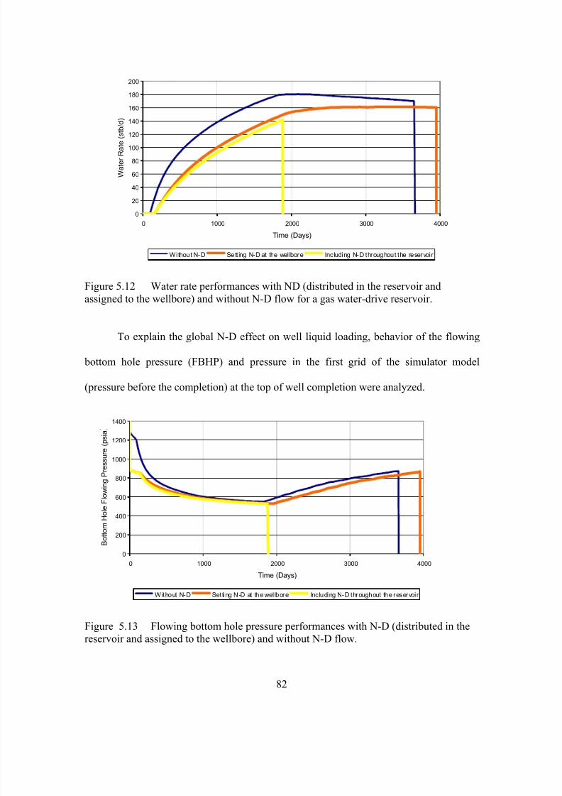
7/23/2019 Armenta Dis
http://slidepdf.com/reader/full/armenta-dis 100/263

7/23/2019 Armenta Dis
http://slidepdf.com/reader/full/armenta-dis 101/263
Figure 5.13 shows that FBHP is always higher when N-D is ignored, which
makes physical sense. Also, FBHP is the same for N-D at the wellbore or distributed
throughout the reservoir. After 1,882 days, however, the well with global N-D stops
producing while the other wells continue with increasing flowing pressure due water
inflow.
0
200
400
600
800
1000
1200
1400
1600
1800
0 1000 2000 3000 4000
Time (Days)
F l o w i n g P r e s s u r e a t t h e S a n d f a c e a t t h e T o
o f C o m p l e t i o n ( p s i a )
Without N-D Setting N-D at the wel lbore Including N-D throughout the reservoir
Figure 5.14 Pressure performances in the first simulator grid (before completion) with
ND (distributed in the reservoir and assigned to the wellbore) and without N-D flow.
Analysis of pressure in the first grid of the simulator model (Figure 5.14) explains
the reason for early termination of production in the gas well with global N-D. Pressure
in the first simulator grid is the pressure before the well completion on the reservoir side.
For the same completion length and gas flow rate, pressure at the first grid of the
simulator should always be lower when N-D is considered. For this example, when N-D
is considered globally, pressure at the first grid of the simulator is always lower than the
non N-D scenario. This is in good agreement with the physical principle explained
83

7/23/2019 Armenta Dis
http://slidepdf.com/reader/full/armenta-dis 102/263
previously. On the other hand, when N-D is set at the wellbore, pressure at the first grid
of the simulator is always higher than the non N-D scenario. This is contrary to the
physical principle explained previously. In short, setting N-D at the wellbore makes the
reservoir gain pressure instead of losing it at the sandface.
1200
1400
1600
1800
2000
2200
2400
0.01 0.1 1 10 100 1000 10000
Distance From the Wellbore (ft)
P r e s s u r e ( p s i )
Without N-D Set ting N-D at the wellbore Including N-D trough the reservoi r
Figure 5.15 Pressure distribution on the radial direction at the lower completion layerafter 126 days of production (Wells produced at constant gas rate of 8.0 MMSCFD) with
ND (distributed in the reservoir and assigned to the wellbore) and without N-D flow.
Figure 5.15 shows the pressure distribution on the radial direction at the lower
completion layer after 126 days of constant gas rate (8.00 MMSCFD) when N-D is
considered globally, assigned only at the wellbore, and without considering N-D. The
effect of N-D extends 6 feet from the wellbore. The main effect, however, happens two
feet around the wellbore. Again, pressure distribution around the wellbore is higher when
N-D is assigned to the wellbore than the case when N-D is ignored showing the
erroneous physical behavior for this condition (N-D set at the wellbore). Pressure at 0.01
ft from the wellbore is 500 psi lower when N-D is considered throughout the reservoir
84

7/23/2019 Armenta Dis
http://slidepdf.com/reader/full/armenta-dis 103/263
than when N-D is ignored. This extra pressure drop in the reservoir makes gas wells
extremely vulnerable to water loading reducing final gas recovery.
From the previous analysis, it is evident that setting N-D at the wellbore to
simulate gas wells’ performance does not properly represent the N-D flow physical
principle. N-D should be distributed throughout the reservoir.
5.4 Results and Discussion
The results of this study emphasize the important physical principle of
considering N-D globally–throughout the reservoir.
Not only gas rate but also porosity and permeability control N-D contribution to
the total pressure drop in gas wells. Contribution of the pressure drop generated by N-D
to the total pressure drop increases when gas rate is increased. Increasing gas rate
increases interstitial gas velocity and the inertial component associated. Reducing
porosity increases contribution of N-D to the total pressure drop. Reduction on porosity
reduces rock-space for the gas to flow increasing, again, gas interstitial velocity.
Reducing permeability increases contribution of N-D to the total pressure drop, also.
Reduction on permeability reduces gas flow ability. At the same gas rate, gas interstitial
velocity increases when permeability is reduced.
The well-accepted assumption in petroleum engineering that assigning N-D at the
wellbore represents this phenomenon is not precise. N-D should be considered globally
throughout the gas reservoir to really evaluate its effect on gas rate and gas recovery.
N-D effect could reduce gas recovery in water-drive gas reservoirs because it
makes the well more sensitive to water loading. Liquid saturation may also increase the
N-D effect (Geertsman, 1974; Evan et al ., 1987; Tiss & Evans, 1989; Frederick &
85

7/23/2019 Armenta Dis
http://slidepdf.com/reader/full/armenta-dis 104/263

7/23/2019 Armenta Dis
http://slidepdf.com/reader/full/armenta-dis 105/263
CHAPTER 6
WELL COMPLETION LENGTH OPTIMIZATION IN GAS RESERVOIRS
WITH BOTTOM WATER
There is a dilemma in the petroleum industry about the completion length to solve
water production in gas wells. A normal practice is to make a short completion at the top
of the gas zone to delay water coning/production. This short completion, however,
reduces gas inflow and delays gas recovery. Recently, some researchers (McMullan &
Bassiouni, 2000; Armenta, White, and Wojtanowicz, 2003) have proposed that a long
completion should be used to increase gas rates and accelerate gas recovery. The previous
analysis, however, did not include the economic implications of completions length in
gas reservoir.
The objective of this study is to examine the factors that control the value of
water-drive gas wells and propose methods to analyze and optimize completion strategy.
Due to the size of the experimental matrix (20,736 results), one committee member (Dr.
Christopher D. White) helped the author building the statistical model and writing the
computer code to run the statistical model.
6.1 Problem Statement
The dependence of recovery on aquifer strength, reservoir properties and
completion properties is complex. Although water influx traps gas, it sustains reservoir
pressure; although limited completion lengths suppress coning, they lower well
productivity. These tradeoffs can be assessed using numerical simulation and discounting
to account for the desirability of higher gas rates.
87

7/23/2019 Armenta Dis
http://slidepdf.com/reader/full/armenta-dis 106/263
6.2 Study Approach
A base model for a single well is specified. Many of the properties of this model
are varied over physically reasonable ranges to determine the ranges of relevant reservoir
responses including ultimate cumulative gas production, maximum gas rate, and
discounted net revenue. The responses are examined using analysis of variance, response
surface models, and optimization.
6.2.1 Reservoir Simulation Model
Numerical reservoir simulators can predict the behavior of complex reservoir-well
systems even if the governing partial differential equations are nonlinear. The same
model explained in section 5.3 was used for the study. The model chosen for this study
used 26 cylinders in the radial direction by 110 layers in the vertical direction (McMullan
& Bassiouni, 2000), providing adequate resolution of near-well coning behavior. The
radius of the gas zone is 2,500 ft, and its thickness is 100 ft. The gas zone has 100 grids
in the vertical direction (one foot per grid). The radius of the water zone is 5,000 ft, and
its thickness is varied from 110 to 1410 ft. The water zone has 10 grids in the vertical
direction. Nine of them have a thickness of 10 ft and the bottom grid is varied to
represent the aquifer. The aquifer is represented by setting porosity to one for the
outermost gridblocks and the thickness of the lowermost gridblocks are varied from 110
to 1410 ft to adjust aquifer volume. The gas-water relative permeability curves are for a
water-wet system (Table 5.4) reported from laboratory data (Cohen, 1989). The gas
deviation factor (Dranchuck et al., 1974) and gas viscosity (Lee et al., 1966) were
calculated using published correlations (Table 5.4). Capillary pressure is neglected (set to
zero), and relative permeability hysteresis is not considered. The well performance was
modeled using the Petalas and Aziz (1997) mechanistic model correlations
88

7/23/2019 Armenta Dis
http://slidepdf.com/reader/full/armenta-dis 107/263
(Schlumberger, 1998). Appendix F includes a sample data deck for the Eclipse reservoir
model. Reservoir properties and economic parameter are the factors varied for the study.
6.2.1.1 Factors Considered
Factors are the parameters that are varied. Five reservoir parameters (initial
pressure, horizontal permeability, permeability anisotropy, aquifer size, and completion
length) and three economic factors (gas price, water disposal cost, and discount rate) are
selected for consideration; each factor is assigned a plausible range. Table 6.1 shows the
factors and the range values for each one.
Table 6.1 Factor descriptions.
Levels
Factor Type Symbol Description Units # L e v e l s
1 2 3 4
pi Initial Pressure psia 3 1500 2300 3000
kh Horizontal Permeability md 3 1 10 100
V AD Aquifer Size ~ 4 100 400 800 1500
Reservoirvariables
kzD Anisotropy Ration ~ 4 0.1 0.3 0.5 1
Cg Gas price $/Mscf 3 1 3.5 6
Cw Water cost $/bbl 3 0.5 1.25 2Economicvariables
d Discount rate annual 4 0 0.06 0.12 0.18
Controllable hpD Completion Fraction ~ 4 0.2 0.5 0.8 1
Factors can be classified by our knowledge and our ability to change them.
Controllable factors can be varied by process implementers. Observable factors can be
measured relatively accurately, but cannot be controlled. Uncertain factors can neither be
measured accurately nor controlled (White & Royer, 2003). For this study, there are four
uncontrollable, uncertain reservoir parameters. Initial pressure (pi ) affects the original
gas in place and the absolute open flow potential of the well (Lee & Wattenbarger, 1996);
it has a less important effect on density contrast. Horizontal permeability (k h ) affects flow
potential and influences coning behavior by altering the near-well pressure distribution
89

7/23/2019 Armenta Dis
http://slidepdf.com/reader/full/armenta-dis 108/263
(Kabir, 1983). Permeability anisotropy (k zD = k z /k h) affects coning and crossflow
behavior Battle & Roberts, 1996), and aquifer size (V AD = W /G) determines the amount
of reservoir energy that can be provided by water drive.
There are three economic parameters. Gas price (C g ) and water disposal cost (C w )
are used to compute the revenues and costs associated directly with production. No
capital costs or other operating costs are considered in this analysis. The discount rate (d )
is used to compute the present value of the gas production less the water disposal costs.
The economic parameters may be difficult to predict, especially gas price. Therefore, it is
reasonable to consider them uncertain and uncontrollable.
The only controllable factor is the completion length (h pD = h p/h). Completion
length should be chosen to minimize water production with acceptable reductions in flow
potential. The completion is assumed to occur over a continuous interval beginning at the
top of the reservoir. The completion length is optimized over the ranges of the uncertain
and/or uncontrollable factors.
6.2.1.2 Responses Considered
Decisions are based on responses obtained by measurement or modeling.
Reservoir studies examine responses that affect project values, e.g., time of water
breakthrough, cumulative recovery (White & Royer, 2003). Three responses were
examined in this study. The ultimate cumulative gas production (G pU ) is the total
undiscounted value of a gas stream, whereas the peak rate (q g,max ) is positively correlated
to the discounted value. Discounted cash flow (N) measures the net present value of the
production stream. The net present value ignores investments and all operating costs
except for water handling.
90

7/23/2019 Armenta Dis
http://slidepdf.com/reader/full/armenta-dis 109/263
6.2.2 Statistical Methods
6.2.2.1 Experimental Design
Experimental design methods have found broad application in many disciplines.
In fact, we may view experimentation as part of the scientific process and as one of the
ways to learn about how systems or process work. Generally, we learn through a series of
activities in which we make conjecture about a process, perform experiments to generate
data from the process, and then use the information from the experiment to establish new
conjectures, which lead to new experiments, and so on (Montgomery, 1997).
The purpose of experimental design is to select experiments to provide
unambiguous, accurate estimates of factor effects with a reasonable number of
experiments. In the context of this study, an “experiment” is a numerical simulation. This
correspondence has been widely used, although there are relevant differences between
physical experiments (with nonrepeatable errors) and numerical simulations (Sacks et al .,
1989).
Because the simulations in this study are relatively inexpensive, a full multilevel
factorial is used (Table 6.1). For the five reservoir and completion parameters, this design
requires 576 simulations. The three economic factors increase the number of results for N
36-fold, to 20,736.
6.2.2.2 Statistical Analyses
Although the number of factors is moderately large (8) and the number of
economic responses to be considered is very large (20,736), this amount of data can be
manipulated using public-domain statistical program ( R ) and commercial spreadsheet
(Microsoft excel) software.
91

7/23/2019 Armenta Dis
http://slidepdf.com/reader/full/armenta-dis 110/263
6.2.2.3 Linear Regression Models
Regression analysis is a statistical technique for investigating and modeling the
relationship between variables (Montgomery & Peck, 1982). The first step in the
statistical analysis of the responses was to formulate a linear model without interaction
among them. This linear model is described by the equation:
0
1
r
i i
i
y x β β =
= + ∑ ……………………………………………………(6.1)
Where there are r=8 factors xi with coefficients β I ; β 0 is the intercept. This
equation is often called a “response surface model” (RSM), or simply a “response
model,” in the context of experimental design. This equation (Eqn. 6.1) was used as the
basis for analysis of variance.
Models with interactions are appropriate when the importance of a factor varies
with the values of other factors (Myers & Montgomery, 2002); for example, the
importance of aquifer size commonly depends on the permeability (White & Royer,
2003). A linear regression model with interaction was developed for the responses. The
interaction terms in a linear model have the form β ij xi x j (Eqn. 6.1) where β ij is the
interaction coefficient between two factors, and xi, x j are factors. The coefficients of linear
models are commonly computed using linear least squares method. The last-squares
criterion is a minimization of the sum of the squared differences between the observed
responses, and the predicted responses for each fixed value of the factor (Jensen et al .,
2000).
Two additional complications were encountered when the linear model with
interactions was built. First, the response variance was not uniform. For example, a
subsample of large aquifer will have a larger volume variance than a subsample of
92

7/23/2019 Armenta Dis
http://slidepdf.com/reader/full/armenta-dis 111/263
smaller aquifer. Such heteroscedacity was eliminated with a variance-stabilizing Box-
Cox transform (Box & Cox, 1964). Second, the responses were not linear with respect to
the factors (or independent variables). This tended to increase estimation error, and could
partly treated using a Box-Tidwell transform on each of the independent variables (Box
& Tidwell, 1962). The resulting form (for a first-order model in the transformed
parameters) is
∑=
+=r
i
b
ii
a x y1
0'' β β ………………………………………..(6.2)
Where a is the Box-Cox power and the bi are the Box-Tidwell powers for each factor.
One must have a large number of experiments to estimate these parameters accurately.
The Box-Cox and Box-Tidwell transforms create a more accurate model that better
conforms to the assumptions of least-squares estimates. In general, untransformed
equations are more useful for discussion and transformed equations are better for
modeling.
6.2.2.4 Analysis of Variance
Analysis of variance (ANOVA) was used to discern which factors are
contributing to the variability of a response. The idea of an analysis of variance is to
express a measure of the total variation of a set of data as a sum of terms, which can be
attributed to specific source, or cause, of variation. ANOVA is an excellent procedure to
use to screen variables and is a standard method for analysis of factorial designs (Myers
& Montgomery, 2002).
6.2.2.5 Monte Carlo Simulation
Monte Carlo is a powerful numerical technique for using and characterizing
random variables in computer programs. If we know the cumulative distribution function
93

7/23/2019 Armenta Dis
http://slidepdf.com/reader/full/armenta-dis 112/263

7/23/2019 Armenta Dis
http://slidepdf.com/reader/full/armenta-dis 113/263

7/23/2019 Armenta Dis
http://slidepdf.com/reader/full/armenta-dis 114/263
6.3 Results and Discussion
6.3.1 Linear Models
Equations 6.3, 6.4, and 6.5 show the linear regression models for the ultimate cumulative
gas production (G pU ), peak gas rate (q g,max), and discounted cash flow ( N ) without
interactions.
zD ADh pDi pu k E V E k E h E p E E G *445.6*328.6*504.1*315.1*403.2698.8 −−+++−= ………………………...(6.3)
zD ADh pDi g k V k h pq *6023.0*0269.0*1670*94.48*425.812750max, +++++−= …………………………….(6.4)
d C C k V k h p N w g zD ADh pDi *0322.0*867.0*2305.0*157.0*0112.0*5265.0*1049.0*0449.054.83 −−+−−+++−= ...(6.5)
G pU increases with initial reservoir pressure, length of completion and horizontal
permeability. G pU decreases with aquifer size and permeability anisotropy (Eqn. 6.3).
The maximum rate q g,max increases with the five reservoir factors included for the
study (Eqn. 6.4).
Finally, N increases with initial reservoir pressure, length of completion,
horizontal permeability, and gas price. N decreases with aquifer size, permeability
anisotropy, water disposal cost, and discount rate (Eqn. 6.5).
The precision of the liner models without interactions is poor; R2 values average
around 0.5 or 0.6. This is not accurate enough for optimization, and improved models
with interactions among the factors are needed.
A more accurate response model is needed to understand response variability and
to optimize. An accurate model for net present value is built by (1) applying a Box-Cox
transform to N , (2) computing maximum likelihood estimates of the Box-Tidwell
transforms (Box & Cox, 1964; Box & Tidwell, 1962), (3) scaling all factors to cover a
unit range, and (4) fitting a model with two-term interactions and quadratic terms.
96

7/23/2019 Armenta Dis
http://slidepdf.com/reader/full/armenta-dis 115/263
Eqns. 6.6 to 6.12 (Table 6.2) show the relationship among the transformed to
untransformed factors where the superscript t denotes the transformed, scaled factor
values.
7.105
90.1687013.0 −= it
i
p p ………………………………………………………(6.6)
787.0
2125.03362.0 −=
−ht
h
k k ………………………………………………………(6.7)
062.0
0585.1024.0 −= zDt
zD
k k ………………………………………………………(6.8)
069.0
0224.0519.0 −=
− ADt
AD
V V …………………………………………………….(6.9)
5
1−=
g t
g
C C ………………………………………………………………(6.10)
5.1
5.0−= wt
w
C C ……………………………………………………………(6.11)
415.0
5135.0d
d t = ………………………………………………………………(6.12)
Table 6.2 Factor descriptions including Box-Tidwell power coefficients
Levels
Factor Type Symbol Description Units # L e v e l s
1 2 3 4
Box-TidwellPower
pi Initial Pressure psia 3 1500 2300 3000 0.70
kh Horizontal Permeability md 3 1 10 100 -0.34
V AD Aquifer Size ~ 4 100 400 800 1500 -0.52
Reservoirvariables
kzD Anisotropy Ration ~ 4 0.1 0.3 0.5 1 0.02
Cg Gas price $/Mscf 3 1 3.5 6 1.00
Cw Water cost $/bbl 3 0.5 1.25 2 1.00Economicvariables
d Discount rate annual 4 0 0.06 0.12 0.18 0.51
Controllable hpD Completion Fraction ~ 4 0.2 0.5 0.8 1 1.39
97
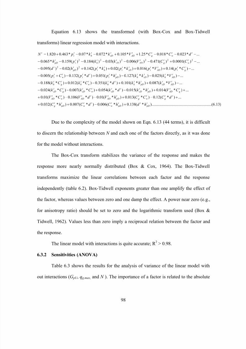
7/23/2019 Armenta Dis
http://slidepdf.com/reader/full/armenta-dis 116/263
Equation 6.13 shows the transformed (with Box-Cox and Box-Tidwell
transforms) linear regression model with interactions.
)13.6.(..................................................).........*(138.0)*(006.0)*(007.0)*(032.0
...)*(12.0)*(013.0)*(01.0)*(106.0)*(01.0
...)*(014.0)*(015.0)*(054.0)*(007.0)*(024.0
...)*(087.0)*(101.0)*(351.0)*(012.0)*(188.0
...)*(025.0)*(127.0)*(051.0)*(132.0)(005.0
...)*(14.0)*(016.0)*(02.0)*(142.0)(02.0)(095.0
...)(0001.0)(471.0)(006.0)(03.0)(184.0)(159.0*065.0
...*023.0*018.0*25.1*105.0*072.0*07.0*463.0820.1
22
222222
t
pD
t t
pD
t
w
t t
w
t
pD
t
g
t t
g
t
w
t
g
t
pD
t
AD
t t
AD
t
w
t
AD
t
g
t
AD
t
pD
t
zD
t t
zD
t
w
t
zD
t
g
t
zD
t
AD
t
zD
t
pD
t
h
t t
h
t
w
t
h
t
g
t
h
t
AD
t
h
t
zD
t
h
t
pD
t
i
t t
i
t
w
t
i
t
g
t
i
t
AD
t
i
t
zD
t
i
t
h
t
i
t
pD
t
t wt g t ADt zDt ht it pD
t t
w
t
g
t
AD
t
zD
t
h
t
i
t
hd hC d C hC
d C C C hV d V C V
C V hk d k C k C k
V k hk d k C k C k
V k k k h pd pC p
C pV pk pk phd
C C V k k ph
d C C V k k p N
+−++
+−+−−+
++−+−−
−++−+−
−−−+−+−
−++++−−
−+−−−−−−
−−−++−−+=
Due to the complexity of the model shown on Eqn. 6.13 (44 terms), it is difficult
to discern the relationship between N and each one of the factors directly, as it was done
for the model without interactions.
The Box-Cox transform stabilizes the variance of the response and makes the
response more nearly normally distributed (Box & Cox, 1964). The Box-Tidwell
transforms maximize the linear correlations between each factor and the response
independently (table 6.2). Box-Tidwell exponents greater than one amplify the effect of
the factor, whereas values between zero and one damp the effect. A power near zero (e.g.,
for anisotropy ratio) should be set to zero and the logarithmic transform used (Box &
Tidwell, 1962). Values less than zero imply a reciprocal relation between the factor and
the response.
The linear model with interactions is quite accurate; R 2
> 0.98.
6.3.2 Sensitivities (ANOVA)
Table 6.3 shows the results for the analysis of variance of the linear model with
out interactions (G pU , q g,max, and N ). The importance of a factor is related to the absolute
98

7/23/2019 Armenta Dis
http://slidepdf.com/reader/full/armenta-dis 117/263
value of its effect. The effect is the change in the response across the range of the factor,
averaged across all levels of other factors.
Table 6.3 Linear sensitivity estimates for models without factors interactions.
Effects of factors across entire range.
G pU q g,max N
F a c t o r
BCF S.C. MMCF/day S.C. MM$ S.C.S.C. or Significance Codes
(ANOVA)
pi 30.49 *** 12.64 *** 0.399 ***
kh 10.33 *** 16.53 *** 0.353 *** Pr(|t|)> Pr(|t|)<= Symbol
kzD -5.81 *** 0.05 -0.101 *** 0 0.001 ***
V AD -8.80 *** 0.04 *** -0.074 *** 0.001 0.01 **
Cg 0.713 *** 0.01 0.05 *
Cw -0.009 ** 0.05 0.1 o
d -0.330 *** 0.1 1 blankhpD -0.09 3.92 *** 0.070 ***
For cumulative gas production, all effects are highly significant except for
completion length, which has a relatively small effect. This weak effect implies that
varying the completion interval has little effect on cumulative production. For maximum
gas rate, all factors have significant effects except for permeability anisotropy. For net
present value, all factors are significant. The effects of gas price, initial pressure,
horizontal permeability, and discount rate dominate other factors; water disposal cost has
a relatively small effect. All effects were computed over the ranges given in table 6.1.
Table 6.4 shows the results for the analysis of variance of the response model
with interactions. The transformed linear model has a large number of terms. ANOVA
shows that 42 of the 44 terms are retained at the 90% level of significance (Eqn. 6.13).
This is a relatively complex response surface. Commercial spreadsheet (Microsoft excel)
was used to evaluate the model.
99

7/23/2019 Armenta Dis
http://slidepdf.com/reader/full/armenta-dis 118/263

7/23/2019 Armenta Dis
http://slidepdf.com/reader/full/armenta-dis 119/263
First, the model was transformed back to the original factors, correcting it for bias
introduced by the back transform from the transformed response N 0.19
to the original
response N (Jensen et. al ., 1987); this correction ranges from about 5 percent at
to less than ½ percent atMM$1= N MM$350= N . Next, graphs of the interaction of N
with respect to the factors were built. Finally, the graphs were analyzed to establish the
response model behavior.
Figures 6.2 to 6.5 show the response model graphs. The combination of
transformations, interactions and a second-order model yields surfaces that are far from
planar (factors not varied are set to their center point value). Visualization of these
surfaces contributes to understanding of the governing factors. Highly nonlinear
functions can be modeled because of the use of the Box-Cox and Box-Tidwell
transforms.
1500
2025
2550
1 1 1
2
1
3
1 4 1 5
1 6 0 7
0 8 0 9
0 1 0 0
0
20
40
60
80
100
120
140
160
180
N
(MM$)
pi (psia)
kh (md)
Figure 6.2 Effects of permeability and initial reservoir pressure on net present value.
101

7/23/2019 Armenta Dis
http://slidepdf.com/reader/full/armenta-dis 120/263
Horizontal permeability is most influential when it is low, and its effect is
comparable to the initial pressure (Figure 6.2).
20
48
76
1 1 1 2
1 3 1 4
1 5 1 6
0 7 0 8
0 9 0
1 0 0
0
20
40
60
80
100
120
140
160
180
N
(MM$)
hpD
(percent)
kh (md)
Figure 6.3 Effects of permeability and completion length on net present value.
The effect of completion length appears small compared with horizontal
permeability (figure 6.3), and the permeability effect is largest at low permeability.
Completion length effect is statistically significant. Although small, the completion
length effect is not negligible (table 6.4).
20
48
76
1 . 0
1 . 5
2 . 0
2 . 5
3 . 0
3 . 5
4 . 0
4 . 5
5 . 0
5 . 5
6 . 0
0
20
40
60
80
100
120
140
160
180
N
(MM$)
hpD
(percent)
Cg ($/MCF)
Figure 6.4 Effects of gas price and completion length on net present value.
102

7/23/2019 Armenta Dis
http://slidepdf.com/reader/full/armenta-dis 121/263
Gas price has a larger effect than the completion length (figure 6.4). The effect of
completion length is greater at high gas price; this is a two-term interaction supporting
the interacting, transformed linear model form.
0
0 . 0
2 7
0 . 0
5 4
0 . 0
8 1
0 . 1
0 8
0 . 1
3 5
0 . 1
6 2
1
3
50
25
50
75
100
125
150
175
200
225
N
(MM$)
d
(fraction)
Cg ($/MCF)
Figure 6.5 Effects of discount rate and gas price on net present value.
Finally, the economic factors have large effects (figure 6.5; note change in N -
axis).
6.3.3 Monte Carlo Simulation
Monte Carlo simulation reveals the overall distribution of a response, helps
analyze sensitivities, and guides optimization (Damsleth et. al., 1992, White & Royer,
2003; White et. al., 2001). To perform Monte Carlo simulation, distributions on all
uncertain factors must be specified. In this study, beta distributions were used for all
factors (figure 6.6, table 6.5).
Beta distributions (Berry, 1996) are simple to manipulate and interpret: as a and b
increase, the distribution gets narrower, if a is larger than b the distribution peak shifts to
103

7/23/2019 Armenta Dis
http://slidepdf.com/reader/full/armenta-dis 122/263
the left. The distributions are easily scaled to fit any range. In the illustrative figure
(figure 6.6), the uniform distributions (both parameters equal to 1) are appropriate for the
controllable variables, whereas distributions with a long positive tail (a>b) are well
suited to approximating factors like permeability. The distributions used in this study are
reasonable, but do not have any verifiable physical meaning. Selection of reasonable
factor distributions is discussed in texts on Bayesian statistics (Berry, 1996).
Table 6.5 Parameters for beta distributions of factors
Factor pi k zD k zD V AD C g C w d h pD
Minimum 1500 1 10 100 1 0.5 0 0.2
Design Maximum 3000 100 100 1500 6 2 0.18 1
a 1 2 1 4 10 20 20 1
Beta Dist b 1 5 1 4 10 20 20 1
0
1
2
3
4
5
6
0 0.2 0.4 0.6 0.8 1
Scaled value of parameter
P r o
b a
b i l i t y D e n s
i t y
a ,b = 20,20
a ,b = 5 ,2
(a ,b )=(4,4)
a ,b = 1,1
Figure 6.6 Beta distributions used for the Monte Carlo simulation.
Using these factor distributions, the distribution of net present value can be
visualized (figure 6.7). Compared to the base case where h pD is allowed to vary randomly
over its entire range, the case with low h pD has a peak at lower N and fewer high N
104

7/23/2019 Armenta Dis
http://slidepdf.com/reader/full/armenta-dis 123/263
values. Similarly, high h pD is associated with higher N . This shows that, on average,
higher h pD yields higher N.
0
0.002
0.004
0.006
0.008
0.01
0.012
0.014
0.016
0.018
0 50 100 150 200 250
Net present value (MM$)
P r o p o r t i o n
maximum hpD
minimum hpD
full range hpD
Figure 6.7 Monte Carlo simulation of the net present value.
The effects of all factors can be examined by setting each of the factors in to their
P 10, P 50, and P 90 values while allowing the other factors to vary according to their
distributions (table 6.6). Unlike the linear sensitivity analysis (earlier), the Monte Carlo
sensitivity (MCS) method incorporates factor value uncertainty in to the analysis. Table
6.6 shows the results.
Table 6.6 Monte Carlo sensitivity estimates.
Variations and Effects on Net Present Value(MM$)
Effects
Factor P10
P50
P90
Linear Quad.
pi 69.1 99.3 122.9 53.79 -6.69
kh 95.0 98.5 100.1 5.16 -1.89
V AD 104.1 97.2 93.2 -10.93 2.83
kzD 100.4 97.5 95.9 -4.51 1.39
Cg 74.4 97.6 121.4 47.00 0.56
Cw 98.3 98.0 97.6 -0.66 0.00
d 101.4 97.8 94.5 -6.86 0.26
hpD 93.8 98.1 102.0 8.27 -0.32
105

7/23/2019 Armenta Dis
http://slidepdf.com/reader/full/armenta-dis 124/263
These results (table 6.6) bear out the importance of initial pressure and gas price.
Compared with the linear sensitivity analysis, MCS estimates lower sensitivity of net
present value to horizontal permeability. The difference is computed from the P 90 to the
P 10 values, which excludes the extremely low permeability values for which the
permeability sensitivity is greatest (figure 6.2). In general, MCS results differ from linear
sensitivity analyses because unlikely values are down-weighted in MCS. The completion
effect from the MCS appears relatively small (but it is the fourth most important factor).
However, increasing the completion length from 28 ( P 10) to 92 ( P 90) percent of the total
interval length increases the average net present value from 93.8 to 102 MM$, a
substantial change (figure 6.8, table 6.6).
90
95
100
105
110
115
120
125
130
135
140
20 40 60 80 100
Completion length (percent)
N e
t p r e s e n
t v a
l u e
( M
M $ )
low d, high pi, kh, and V AD
base case
optima
Figure 6.8 Optimization of net present considering uncertainty in reservoir andeconomic factors (two cases).
106

7/23/2019 Armenta Dis
http://slidepdf.com/reader/full/armenta-dis 125/263
6.3.4 Optimization
Development teams seek to choose the optimum well configuration for the
prevailing reservoir properties and operating conditions. Response models can be used
for this optimization.
One approach is to differentiate the response model for the objective function
with respect to the controllable parameter, set it equal to zero, and solve for the
controllable parameter (White & Royer, 2003). Here, the model for net present value (Eq.
6.13) is differentiated with respect to the completion length h pD, the differenciate
equation set equal to zero, and then solved for h pD. Eqn. 6.14 shows the resulting
correlation to maximize net present value for any combination of the other parameters.
This correlation is not a function of completion length. This is a mathematical equation
resulting from the statistical function derived for Net Present Value.
635.1481.3150.0803.0254.0372.0550.2294,1, −+−+−−+= t t
w
t
g
t
AD
t
zD
t
h
t
i
t
opt pD d C C V k k ph …….(6.14)
Where the superscript t denotes the transformed, scaled factor values. The effects
of these factors are difficult to interpret because of the Box-Tidwell powers (table 6.2),
but the function can be to evaluate to aid understanding (Roman, 1999). The equations
relating transformed to untransformed factors are given in item 6.3.1 (Eqns. 6.6 to 6.12).
Several observations can be made from Eqn. 6.14: as the initial pressure,
permeability anisotropy and water cost increase, the optimal interval is decreased (These
factors have positive Box-Tidwell power coefficient and negative coefficient in Eq. 6.14).
As the gas price and discount rate increase, motivating higher rates, the optimal interval
107

7/23/2019 Armenta Dis
http://slidepdf.com/reader/full/armenta-dis 126/263
increases (both factors have positive Box-Tidwell power coefficient and positive
coefficient in Eq. 6.14).
Comparison among optimum completion length calculated using Eqn. 6.14 and
fitting responses directly from the data was done, getting good agreement among them
(figure 6.9).
0
20
40
60
80
100
120
0 20 40 60 80 100
Horizonal permeability (md)
O p
t i m a
l c o m p
l e t i o n
l e n
g t h ( p e r c e n
t )
Using Eqn. (3)
Directly fit response surface
Figure 6.9 Optimal completion length calculated from the transformed model and a
response model computed from local optimization.
6.4 Implications for Water-Drive Gas Wells
The statistical and optimization analyses shed light on the general problem of gas
completions in the presence of water drives. Aquifer size is the third most important
factor after initial pressure and gas price (table 6.6). Furthermore, the optimal completion
length was often the full interval, even in the presence of large aquifers and higher-than-
average water costs (figure 6.9).
The optimization from the response model (Eqn. 6.14) is evaluated by comparison
with directly simulated results (Figure 6.9), confirming that the optimum completion
108

7/23/2019 Armenta Dis
http://slidepdf.com/reader/full/armenta-dis 127/263

7/23/2019 Armenta Dis
http://slidepdf.com/reader/full/armenta-dis 128/263

7/23/2019 Armenta Dis
http://slidepdf.com/reader/full/armenta-dis 129/263
water coning in gas wells was different than that in oil wells. Therefore, a specific design
of DWS for gas wells was to be different than for oil wells. Three different possible
configurations were evaluated:
• Dual completion without a packer;
• Dual completion with a packer;
• Dual completion with a packer and gravity gas-water separation.
7.1.1 Dual Completion without Packer
Figure 7.1 depicts the DWS configuration including two completions without a
packer.
Gas
Water
Water
Figure 7.1 Dual completion without packer.
For this configuration, one completion is located at the top of the gas zone.
Another is located in the water zone. Gas is produced from the top completion and water
111

7/23/2019 Armenta Dis
http://slidepdf.com/reader/full/armenta-dis 130/263
from the bottom completion. A pump is located below the lower completion to drain the
water zone and inject the water into a lower disposal zone. This pump generates an
inverse gas cone. Also, the bottom hole pressure at the gas and water completion is the
same.
This configuration gives partial control over the water coning, although some
water is still produced with the gas. The control efficiency, however, would be reduced
with time because (as the gas-water contact moved upward) the amount of water
produced from the top completion would increase and eventually kill the gas production.
The solution here would be a bigger water pump. However, higher pump rate
means the bottom-hole pressure is reduced with time while the amount of water produced
from the top completion increases at the same time. This combination makes the well
very sensitive to liquid loading. In short, this configuration could kill the well early. So, it
would be better to have the two completions isolated to control the vertical movement of
gas-water contact outside the well.
7.1.2 Dual Completion with Packer
Figure 7.2 depicts the DWS configuration with two completions separated with a
packer. The objective is to isolate the bottomhole pressure for the two completions.
Isolating the bottomhole pressure would allow the pump rate to increase when the gas-
water contact moves up without making the well too sensitive to water loading.
Eventually, some water would be produced to the surface from the top completion at later
times.
This configuration allows for better control of water coning in gas wells with time
because it allows two different values of the bottom hole flowing pressures. The top
completion could keep producing gas longer with a small amount of water or even water-
112
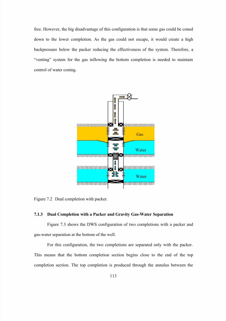
7/23/2019 Armenta Dis
http://slidepdf.com/reader/full/armenta-dis 131/263
free. However, the big disadvantage of this configuration is that some gas could be coned
down to the lower completion. As the gas could not escape, it would create a high
backpressure below the packer reducing the effectiveness of the system. Therefore, a
“venting” system for the gas inflowing the bottom completion is needed to maintain
control of water coning.
Gas
Water
Water
Figure 7.2 Dual completion with packer.
7.1.3 Dual Completion with a Packer and Gravity Gas-Water Separation
Figure 7.3 shows the DWS configuration of two completions with a packer and
gas-water separation at the bottom of the well.
For this configuration, the two completions are separated only with the packer.
This means that the bottom completion section begins close to the end of the top
completion section. The top completion is produced through the annulus between the
113
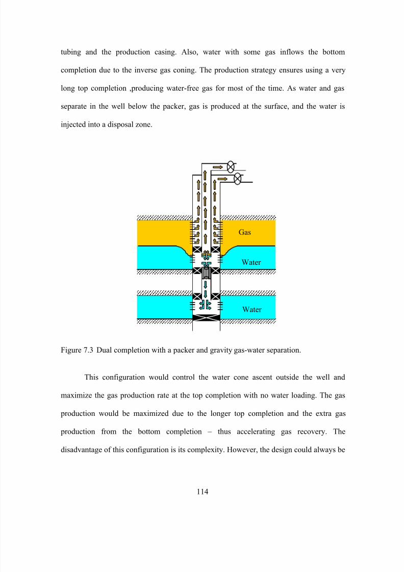
7/23/2019 Armenta Dis
http://slidepdf.com/reader/full/armenta-dis 132/263

7/23/2019 Armenta Dis
http://slidepdf.com/reader/full/armenta-dis 133/263
made simple if the water from the bottom completion was lifted to the surface with the
small amount of gas.
From this qualitative analysis the author selected this design (dual completion
with a packer and gravity gas-water separation) as the best configuration of DWS for gas
wells.
7.2 Comparison of Conventional Wells and DWS Wells
7.2.1 Reservoir Simulator Model
Numerical reservoir simulators can predict the behavior of complex reservoir-well
systems even if the governing partial differential equations are nonlinear. This method
was chosen for this study for several reasons.
• Water production in gas reservoirs is a complex problem.
• Water-drive gas reservoirs have two flowing phases, and it is difficult to
analyze this behavior analytically. Actually, there is no analytical model for
water coning in gas wells.
• The gas-water contact location is dynamic, further complicating analysis.
• Modern reservoir simulators (Schlumberger, 1997) integrate reservoir
inflow and tubing outflow models, which is a vital component of gas well
performance prediction (Lee & Wattenbarger, 1996).
A comparison of gas recovery for conventional and DWS wells was performed
using a gas reservoir model shown in Figure 7.4. The “layer cake-type” model consists of
a gas reservoir on the top of an aquifer (McMullan & Bassiouni, 2000). The radius of the
gas zone is 2,500 ft, and its thickness is 100 ft. The gas zone has 100 grids in the vertical
direction (one foot per grid). The radius of the water zone is 5,000 ft, and its thickness is
800 ft. The water zone has 10 grids in the vertical direction. Nine of them have a
115

7/23/2019 Armenta Dis
http://slidepdf.com/reader/full/armenta-dis 134/263

7/23/2019 Armenta Dis
http://slidepdf.com/reader/full/armenta-dis 135/263
7.2.2 Reservoir Parameters Selection
Vertical permeability and aquifer size were selected to create a well-reservoir
system with severe water problems. Vertical permeability increases water coning in gas
wells; the higher the vertical permeability is, the more severe the coning becomes
(Beattle & Roberts,1996; Armenta & Wojtanowicz, 2002). A reasonable assumption in
petroleum engineering is that vertical permeability is ten-fold smaller than horizontal
permeability. To create a scenario of severe water coning, vertical permeability was
assumed to be fifty percent of horizontal.
Textbook models of water inflow for material balance computations assume that
the amount of water encroachment into the reservoir is related to the aquifer size (Craft &
Hawkins, 1991). (For example, van Everdinger and Hurst used the term B’ representing
the volume of aquifer. The Fetkovich model considers a factor called W ei defined as the
initial encroachable water in place at the initial pressure.) For this study, we assumed that
the pore volume of the aquifer is 968–fold greater than the gas pore volume a condition
of strong bottom water drive.
The inflow gas rate depends on reservoir permeability, so the rate of recovery is
controlled by the gas rate. Three values of permeability, 1, 10, and 100 md, were selected
for this study.
Water loading kills gas wells causing reduced gas recovery; initial reservoir
pressure plays an important role in this process. To investigate this effect, three different
initial reservoir pressures were considered: low (subnormal), normal, and high
(abnormal). Typically, reservoirs with an initial pressure gradient between 0.43 and 0.5
psi/ft are considered normally pressured (Lee & Wattenbarger, 1996). For this study, the
initial reservoir pressure was calculated assuming 0.3 psi/ft, 0.46 psi/ft, and 0.6 psi/ft
117

7/23/2019 Armenta Dis
http://slidepdf.com/reader/full/armenta-dis 136/263
values of pore pressure gradients for the subnormal, normal, and abnormal reservoir,
respectively.
Gas recovery from certain water-drive gas reservoirs may be very sensitive to gas
production rate. If practical, the field should be produced at as high a rate as possible.
This may result in a significant increase in gas reserves by lowering the abandonment
pressure (Agarwal et al., 1965).
Simulations for conventional wells were run at constant tubing head pressure
(THP) of 300 psi at a maximum gas rate for the THP.
The DWS well was modeled assuming two wells at the same location; the top-
completion well was produced the same way as the conventional well. The bottom-well
completion was also run at constant THP (300 psi) until there was no more gas inflow to
the bottom completion. Then, the bottom-completion well was produced at a constant
maximum water rate. The length of the bottom completion for the DWS well was set at
30% the length of the top completion.
7.2.3 Conventional Wells Completion Length
The potential benefit of long completion length to increase net present value in
gas wells was identified in Chapter 6. This result agrees with detailed studies of
completion length in gas reservoirs (McMullan & Bassiouni, 2000). For this study, the
well completion length of conventional wells was selected to maximize gas recovery. The
selection was needed to provide an unbiased comparison of the single – and dual –
completed wells and to investigate if DWS gives some extra recovery beyond the
maximum recovery of conventional wells.
The effect of completion length on recovery was simulated for different initial
reservoir pressure and permeability.
118

7/23/2019 Armenta Dis
http://slidepdf.com/reader/full/armenta-dis 137/263
510
3050
70100
k = 1 md
k = 10 md
k = 100 md0
10
20
30
40
50
60
70
80
G a s R e c o v
e r y ( % )
Fraction of Gas Zone Perforated (%)
Figure 7.5 Gas recovery for different completion length in gas reservoirs with subnormalinitial pressure.
Figure 7.5 shows the results for a gas reservoir with subnormal initial reservoir.
Gas recovery increases with permeability. Also, for each permeability value, the
maximum recovery occurs when the gas zone is totally perforated.
510
3050 70
100
k =1 md
k =10 md
k =100 md0
10
20
30
40
50
60
70
G a s R e c o v e r y ( % )
Fraction of Gas Zone Perforated (%)
Figure 7.6 Gas recovery for different completion length in gas reservoirs with normal
initial pressure.
119
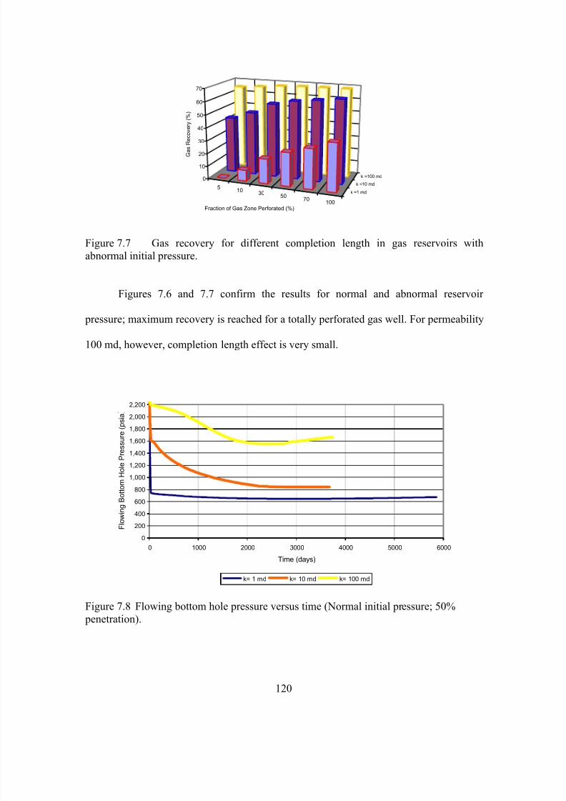
7/23/2019 Armenta Dis
http://slidepdf.com/reader/full/armenta-dis 138/263
510
3050
70100
k =1 md
k =10 md
k =100 md0
10
20
30
40
50
60
70
G a s R e
c o v e r y ( % )
Fraction of Gas Zone Perforated (%)
Figure 7.7 Gas recovery for different completion length in gas reservoirs with
abnormal initial pressure.
Figures 7.6 and 7.7 confirm the results for normal and abnormal reservoir
pressure; maximum recovery is reached for a totally perforated gas well. For permeability
100 md, however, completion length effect is very small.
0
200
400
600
800
1,000
1,200
1,400
1,600
1,800
2,000
2,200
0 1000 2000 3000 4000 5000 6000
Time (days)
F l o w i n g B o t t o m H o l e P r e s s u r e ( p s
i a
k= 1 md k= 10 md k= 100 md
Figure 7.8 Flowing bottom hole pressure versus time (Normal initial pressure; 50%
penetration).
120

7/23/2019 Armenta Dis
http://slidepdf.com/reader/full/armenta-dis 139/263
The finding can be explained as follows. Gas recovery increases with
permeability because of the larger gas rate and higher flowing bottom hole pressure. The
well can tolerate higher water rates before loading up with liquid. Moreover, gas recovery
is faster at high gas rates.
0
5,000
10,000
15,000
20,000
25,000
30,000
0 1000 2000 3000 4000 5000 6000
Time (days)
G a s R a t e ( M s c f / D )
k= 1 md k= 10 md k= 100 md
Figure 7.9 Gas rate versus time (Normal initial pressure; 50% penetration).
Figures 7.8, and 7.9 support these observations. (They show the results for the
normal initial reservoir pressure with 50% gas zone penetration.) They show the highest
flowing pressure and gas rate for permeability 100 md.
Overall, shorter completion length gives longer production time for conventional
wells.
From this study, it is possible to conclude that the highest gas recovery is when
the gas zone is totally perforated, particularly for permeability 1 and 10 md. For
permeability 100 md, gas recovery is almost insensitive to length of perforation.
121
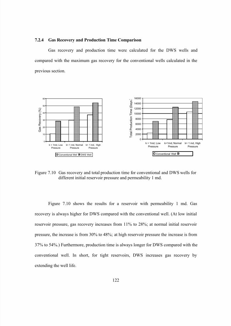
7/23/2019 Armenta Dis
http://slidepdf.com/reader/full/armenta-dis 140/263
7.2.4 Gas Recovery and Production Time Comparison
Gas recovery and production time were calculated for the DWS wells and
compared with the maximum gas recovery for the conventional wells calculated in the
previous section.
Figure 7.10 Gas recovery and total production time for conventional and DWS wells fordifferent initial reservoir pressure and permeability 1 md.
Figure 7.10 shows the results for a reservoir with permeability 1 md. Gas
recovery is always higher for DWS compared with the conventional well. (At low initial
reservoir pressure, gas recovery increases from 11% to 28%; at normal initial reservoir
pressure, the increase is from 30% to 48%; at high reservoir pressure the increase is from
37% to 54%.) Furthermore, production time is always longer for DWS compared with the
conventional well. In short, for tight reservoirs, DWS increases gas recovery by
extending the well life.
0
10
20
30
40
50
60
k = 1md, Low
Pressure
k= 1 md, Normal
Pressure
k= 1 md, High
Pressure
G a s R e c o v e r y
( % )
Conventional Well DWS Well DWS Well
0
2000
4000
6000
8000
10000
12000
14000
16000
k = 1md, Low
Pressure
k=1md, Normal
Pressure
k= 1 md, High
Pressure
T o t a l P r o d u c t i o n T i m e ( D a y s
Conventional Well
122
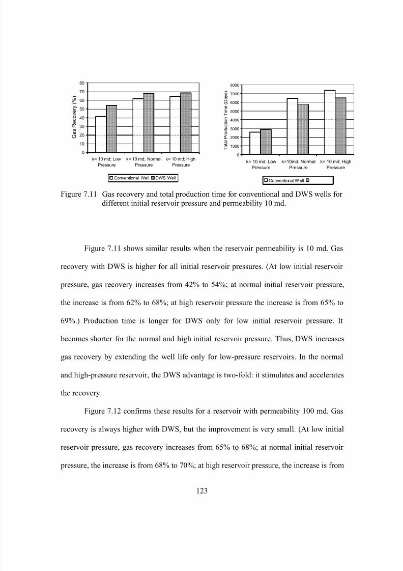
7/23/2019 Armenta Dis
http://slidepdf.com/reader/full/armenta-dis 141/263

7/23/2019 Armenta Dis
http://slidepdf.com/reader/full/armenta-dis 142/263

7/23/2019 Armenta Dis
http://slidepdf.com/reader/full/armenta-dis 143/263
0
500
1,000
1,500
2,000
2,500
3,000
0 1000 2000 3000 4000 5000 6000 7000
Time (Days)
G a s R a t e ( M s c f / D )
DWS-Top Complet ion Convent ional
Figure 7.13 Gas rate history for conventional and DWS wells (Subnormal reservoir
pressure and permeability 1 md).
0
100
200
300
400
500
600
700
800
0 1000 2000 3000 4000 5000 6000 7000
Time (Days)
B o t t o m F l o w i n g P r e s s u r e ( p s i a
DWS-Top Completion Convent ional
Figure 7.14 Flowing bottom hole pressure history for conventional and DWS wells
(Subnormal reservoir pressure and permeability 1 md).
125

7/23/2019 Armenta Dis
http://slidepdf.com/reader/full/armenta-dis 144/263
Figure 7.13 shows gas rate versus time for the conventional and DWS well. The
gas rate is always higher for DWS because the top completion produces almost water free
most of the time.
Figure 7.14 shows flowing bottom hole pressure of the wells. It shows that the
bottom hole flowing pressure increase is slower for DWS than for conventional wells. In
short, removing the water inflow to the top completion delays liquid loading of the well
and elevates production rate.
From this study, one could conclude that the best reservoir conditions for DWS
would be low-permeability low-pressure gas reservoirs. With conventional technology,
such reservoirs necessitate the use of a lifting technology (i.e. DGWS) to produce gas and
water.
7.3 Comparison of DWS and DGWS
The comparison is made for a gas reservoir with low permeability (1 md) and
subnormal initial pressure. This is the worst-case scenario for conventional gas recovery,
identified in the previous section, where there is a need for DWS or other (DGWS)
technology.
7.3.1 DWS and DGWS Simulation Model
The reservoir simulator model described in section 7.2.1 was also used in this
study.
DWS was simulated using two different wells located at the same place, but with
different completion length and depth. The wells represented the top and bottom
completions of DWS wells. Also, two cases of completion length were considered. In the
first case, the top DWS completion totally penetrates the gas zone (100 ft), and the
bottom completion is 30 feet long with the top located one foot below the bottom of the
126

7/23/2019 Armenta Dis
http://slidepdf.com/reader/full/armenta-dis 145/263
top completion (DWS-1). (The same configuration was used to compare DWS with
conventional wells.) In the second case, the top and bottom completion length are 70 and
60 feet, respectively (DWS-2). The two wells representing DWS completions produce
simultaneously at constant THP (300 psia). It is assumed that the tubing of the bottom
completion would only produce gas liberated from water (The Tubing Performance
Relationship curves were built for zero water cut condition, only. Bottomhole flowing
pressure for the bottom conditions is controlled by the THP and the gas friction losses,
only. Both, gas and water, are produced from the reservoir and separated at the wellbore).
When the bottom completion stops producing gas, the well is switched to produce at a
constant and maximum water rate.
DGWS was simulated using two different wells at the same place, too. The two
wells had the same completion length and location. One well represents the situation until
the well loads up with water. At this time the first well is shut down and the second well
takes over. The second well models removal of water by downhole separator (DGWS),
i.e. water free production of gas. Both wells are produced at constant THP (300 psia). It is
assumed that the DGWS well produces gas free of water all the time. This is the best
operational performance of DGWS. Two cases with different completion length were
also considered; totally penetrated gas zone (DGWS-1) and 70% penetration (DGWS-2).
Finally, the economic limit of 400Mscfd was set for the DGWS and DWS wells.
Appendix F includes a sample data deck for the Eclipse reservoir model.
7.3.2 DWS vs. DGWS–Comparison Results
Figures 7.15, 7.16, 7.17, and 7.18 summarize the results of the comparison
between DWS and DGWS.
127

7/23/2019 Armenta Dis
http://slidepdf.com/reader/full/armenta-dis 146/263
0
5
10
15
20
25
30
35
40
45
Gas Zone Totally
Perforated
Gas Zone 70%
Perforated
G a s R e c o v e r y ( % )
Conventional DGWS
0.0
1.0
2.0
3.0
4.0
5.0
6.0
7.0
Gas Zone Totally
Perforated
Gas Zone 70%
Perforated P T R [ ( P r o d u c t i o n T i m e C o n v e n t i o n a l , D W S , o r D G W S ) /
( P r o d u c t i o n T i m e C o
n v e n t i o n a l ) ]
Conventional DGWS
DWS DWS
Figure 7.15 Gas recovery and Production Time Ratio (PTR) for conventional, DWS, and
DGWS wells.
Figure 7.15 shows gas recovery and Production Time Ratio (PTR) for the two
cases of well completion.
al convention
DGWS DWS
TpTp PTR
)()( /
= …………………………………………………………..(7-1)
Where:
PTR = Production time ratio,
(Tp) DWS = Production time for DWS wells,
(Tp) DGWS = Production time for DGWS wells,
(Tp)conventional = Production time for conventional wells.
Figure 7.15 shows that DGWS gives the highest gas recovery (41.5%) when the
gas zone is totally penetrated, and DWS gives the highest recovery (40.7%) when 70% of
the gas zone is penetrated. Thus, maximum recovery for DWS and DGWS is almost the
128

7/23/2019 Armenta Dis
http://slidepdf.com/reader/full/armenta-dis 147/263
same. Moreover, the PTR are 7.4 and 3.5 for DGWS and DWS, respectively. This means
that the same recovery with DGWS takes (6.4/3.5 = 1.83) 1.83 times longer than that
with DWS.
0
5
10
15
20
25
30
35
40
45
0 3000 6000 9000 12000 15000 18000 21000
Time (Days)
G a s R e c o v e r y ( % )
DWS-2 DWS-1 DGWS-2 DGWS-1 Conventional Well-1
Conventional
DGWS-2
DGWS-1DWS-2
DWS-1
Figure 7.16 Gas recovery versus time for DWS, DGWS, and conventional wells.
Figure 7.16 gives gas recovery versus time for the wells in all the cases. The
DGWS-1 and DWS-2 designs give maximum final recoveries that are almost equal.
However, DGWS-1 produces 50% longer than DWS-2. Thus, DWS-2 accelerates gas
recovery. One additional observation for DWS is that reducing the length of the top
completion and increasing the length for the bottom completion would increase gas
recovery by 49% (from 27.3% to 40.7%). This is an important observation because it
shows that completion lengths for DWS should be optimized (Armenta & Wojtanowicz,
2003).
129

7/23/2019 Armenta Dis
http://slidepdf.com/reader/full/armenta-dis 148/263
0
500
1,000
1,500
2,000
2,500
3,000
0 3000 6000 9000 12000 15000 18000 21000
Time (Days)
G a s R a t e ( M
s c f / d )
Conventional Well-1 DGWS-1 DWS-2 Top DWS-2 Bottom
Conventional
DGWS-1
DWS-2 Top
DWS-2 Bottom
Figure 7.17 Gas rate history for DWS-2, DGWS-1, and conventional wells.
0
10
20
30
40
50
60
70
80
90
0 3000 6000 9000 12000 15000 18000 21000
Time (Days)
W a t e r R a t e ( s t b / d )
Conventional Well-1 DGWS-1 DWS-2 Top DWS-2 Bottom
Conventional
DGWS-1
DWS-2 Top
DWS-2 Bottom
Figure 7.18 Water rate history for DWS-2, DGWS-1, and conventional wells.
130

7/23/2019 Armenta Dis
http://slidepdf.com/reader/full/armenta-dis 149/263

7/23/2019 Armenta Dis
http://slidepdf.com/reader/full/armenta-dis 150/263
132
hole pressure for the DWS well is always deferent for the two completions. This
difference is dramatically bigger when the top completion is set to produce at the
maximum water rate releasing the THP restriction for the bottom completion (after 4000
days). This situation would not be possible without a packer. Therefore, as it was
mentioned in section 7.1.3, the packer is needed to guarantee isolation between the two
completions. This isolation is still possible when the two completions are one after the
other (this is the case) giving a better control on the water coning.
From this study, one can say that for the reservoir model used here, DGWS and
DWS could give almost the same final gas recovery, but DWS production time is 35 %
shorter than that for the DGWS well. DWS well, however, would produce little water at
the surface from the top completion, but DGWS well would not lift any water. A packer
between the two completions for the DWS wells is very important giving insulations
between the completions and improving control on the water coning.

7/23/2019 Armenta Dis
http://slidepdf.com/reader/full/armenta-dis 151/263
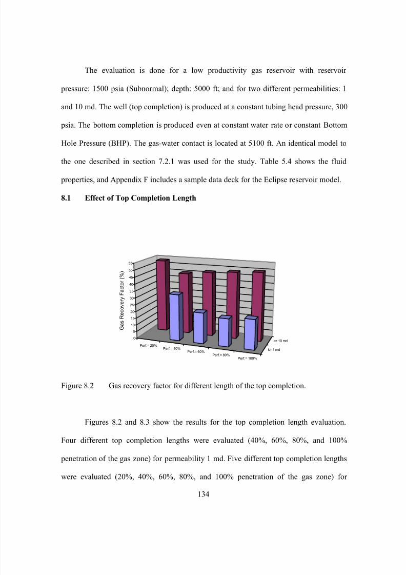
7/23/2019 Armenta Dis
http://slidepdf.com/reader/full/armenta-dis 152/263
The evaluation is done for a low productivity gas reservoir with reservoir
pressure: 1500 psia (Subnormal); depth: 5000 ft; and for two different permeabilities: 1
and 10 md. The well (top completion) is produced at a constant tubing head pressure, 300
psia. The bottom completion is produced even at constant water rate or constant Bottom
Hole Pressure (BHP). The gas-water contact is located at 5100 ft. An identical model to
the one described in section 7.2.1 was used for the study. Table 5.4 shows the fluid
properties, and Appendix F includes a sample data deck for the Eclipse reservoir model.
8.1 Effect of Top Completion Length
Perf.= 20%Perf.= 40%
Perf.= 60%Perf.= 80%
Perf.= 100%
k= 1 md
k= 10 md0
5
10
15
20
25
30
35
40
45
50
55
G a s R e c o v e r y F a c t o r ( % )
Figure 8.2 Gas recovery factor for different length of the top completion.
Figures 8.2 and 8.3 show the results for the top completion length evaluation.
Four different top completion lengths were evaluated (40%, 60%, 80%, and 100%
penetration of the gas zone) for permeability 1 md. Five different top completion lengths
were evaluated (20%, 40%, 60%, 80%, and 100% penetration of the gas zone) for
134

7/23/2019 Armenta Dis
http://slidepdf.com/reader/full/armenta-dis 153/263
permeability 10 md. Bottom completion is located at the top of the aquifer (at 5100 ft)
penetrating 20 ft of the water zone. The bottom completion length (20 ft) was constant
for each case. Constant water-drainage rate from the bottom completion was used (30 bpd
for permeability 1 md, and 200 bpd for permeability 10 md) for each case (Table 8.1).
Perf.=
40%Perf.=
60%Perf.=
80%Perf.=
100%
0
3,000
6,000
9,000
12,000
15,000
T o t a l P r o d u c t i o n T i m e ( D a y s )
Permeability= 1 md
Perf.=
20%Perf.=
40%Perf.=
60%Perf.=
80%Perf.=
100%
0
1,000
2,000
3,000
4,000
5,000
T o t a l P r o d u c t i o n T i m e ( D a y s )
Permeability: 10 md
Figure 8.3 Total production time for different length of the top completion.
135

7/23/2019 Armenta Dis
http://slidepdf.com/reader/full/armenta-dis 154/263

7/23/2019 Armenta Dis
http://slidepdf.com/reader/full/armenta-dis 155/263

7/23/2019 Armenta Dis
http://slidepdf.com/reader/full/armenta-dis 156/263
Table 8.2 shows the operational conditions for the water-drained evaluation, and
Figures 8.4 and 8.5 show the results for this analysis.
Qw= 10
bpd
Qw= 20
bpdQw= 30
bpd Qw=Max
(32-39
bpd)
Qw=
100 bpdQw=
200 bpdQw=
300 bpdQw=
Max
(300-
400 bpd)
k= 1 md
k= 10 md
0
5
10
15
20
25
30
35
40
45
50
55
60
G a s R e c o v e r y F a c t o r ( %
Figure 8.4 Gas recovery factor for different water-drained rate.
Qw= 10
bpdQw= 20
bpdQw= 30
bpdQw= Max
(32-39
bpd)
0
4,000
8,000
12,000
16,000
T o t a l P r o d u c t i o n T i m e ( D a y s )
Permeability: 1 md
Qw= 100
bpdQw= 200
bpd
Qw= 300
bpd Qw= Max(300-400
bpd)
0
1,000
2,000
3,000
4,000
5,000
T o t a l P r o d u c t i o n T i m e ( D a y s )
Permeability: 10 md
Figure 8.5 Total production time for different water-drained rate.
138

7/23/2019 Armenta Dis
http://slidepdf.com/reader/full/armenta-dis 157/263
Gas recovery increases with water-drained rate. The maximum recovery occurs at
the maximum water-drainage rate (Figure 8.4). The effect of water drained in gas
recovery follows the same pattern on both permeabilities. Production time increases with
water-drained rate, also. The longest production time happens at the maximum water-
drainage rate (Figure 8.5). Increasing water-drained rate for permeability 10 md extends
the well life, however, the effect of water drained on total production time is small; It
means that increasing water-drained rate has a dual effect on gas recovery: increases, and
accelerates it at the same time.
Removing water from the top completion delays liquid loading of the well. In
short, the more water is removed from the top completion, the higher and faster/longer
the gas recovery.
8.3 Effect of Separation between the Two Completions
Table 8.3 Operation conditions for evaluation of separation between thecompletions.
Permeability 1 md Permeability 10 md
Separationbetween thecompletions
% of gaszone
penetrated
Length /Location -
TopComp. (ft)
Length /Location -
BottomComp.(ft)
WaterRate
(STB/D)
Separationbetween thecompletions
% of gaszone
penetrated
Length /Location -
TopComp. (ft)
Length /Location -
BottomComp.(ft)
WaterRate
(STB/D)
0 ft 60% 40 /(5000-5040)
20 / (5041-5060)
15 0 ft 40% 20 /(5000-5020)
20 / (5021-5040)
150
20 ft 60% 40 /(5000-5040)
20 / (5060-5080)
15 20 ft 40% 20 /(5000-5020)
20 / (5040-5060)
150
40 ft 60% 40 /(5000-5040)
20 / (5080-5100) 15 40 ft 40% 20 /(5000-5020)
20 / (5060-5080) 150
60 ft 40% 40 /(5000-5040)
20 / (5100-5120)
15 60 ft 40% 20 /(5000-5020)
20 / (5080-5100)
150
80 ft 20% 20 /(5000-5020)
20 / (5100-5120)
150
139

7/23/2019 Armenta Dis
http://slidepdf.com/reader/full/armenta-dis 158/263
Four (for permeability 1md) and five (for permeability 10 md) different
separation distances between the two completions were evaluated. The top completion
length was constant, perforating 40% (permeability 1 md) and 20% (permeability 10 md)
of the gas zone. Top and bottom completion produced gas from day one. The water-
drainage rate was constant (15 bpd for permeability 1 md and 150 bpd for permeability
10 md) once the bottom completion started producing water (Table 8.3). Figures 8.6 and
8.7 show the results for the evaluation of separation distance between the two
completions.
Separ.= 0 ftSepar.= 20 ft
Separ.= 40 ftSepar.= 60 ft
Separ.= 80 ft
k= 1 md
k= 10 md0
5
10
15
20
25
30
35
40
45
50
55
G a s
R e c o v e r y F a c t o r ( % )
Figure 8.6 Gas recovery factor for different separation distance between thecompletions.
Gas recovery reduces with the separation between the two completions (Figure
8.6). The highest recovery occurs when the two completions are one after the other. Both
permeabilities values (1 md and 10 md) show the same pattern. Reducing separation
between the completions increases gas recovery because the inverse gas-cone to the
140

7/23/2019 Armenta Dis
http://slidepdf.com/reader/full/armenta-dis 159/263
bottom completion is more efficient. The reverse gas-cone is needed on the DWS
completion to guarantee water-free production of the top completion.
Separ.= 0
ftSepar.=
20 ftSepar.=
40 ftSepar.=
60 ft
0
2,000
4,000
6,000
8,000
10,000
12,000
14,000
16,000
T o t a l P r o d u c t i o n T i m e ( D a y s )
Permeability 1 md
Separ.=
0 ftSepar.=
20 ftSepar.=
40 ftSepar.=
60 ftSepar.=
80 ft
0
1,000
2,000
3,000
4,000
5,000
6,000
T o t a l P r o d u c t i o n T i m e ( D a y s )
Permeability 10 md
Figure 8.7 Total production time for different separation distance between thecompletions.
DWS extends the well life longer when the two completions are together, also
(Figure 8.7). Delaying water inflows to the top completion retards well liquid loading.
At DWS wells, bottomhole flowing pressure is always different for the two
completions (Section 7.3.3) particularly when the water-drained rate is maximized. The
fact that the two completion are one the other does not change this situation (Figure
7.19).
8.4 Effect of Bottom Completion Length
Four (for permeability 1md) and five (for permeability 10 md) different lengths
for the bottom completion were evaluated. The top completion length was constant,
perforating 40% (permeability 1 md) and 20% (permeability 10 md) of the gas zone. The
141
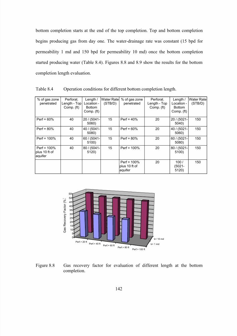
7/23/2019 Armenta Dis
http://slidepdf.com/reader/full/armenta-dis 160/263
bottom completion starts at the end of the top completion. Top and bottom completion
begins producing gas from day one. The water-drainage rate was constant (15 bpd for
permeability 1 md and 150 bpd for permeability 10 md) once the bottom completion
started producing water (Table 8.4). Figures 8.8 and 8.9 show the results for the bottom
completion length evaluation.
Table 8.4 Operation conditions for different bottom completion length.
% of gas zonepenetrated
Perforat.Length - Top
Comp. (ft)
Length /Location -
BottomComp. (ft)
Water Rate(STB/D)
% of gas zonepenetrated
Perforat.Length - Top
Comp. (ft)
Length /Location -
BottomComp. (ft)
Water Rate(STB/D)
Perf = 60% 40 20 / (5041-5060)
15 Perf = 40% 20 20 / (5021-5040)
150
Perf = 80% 40 40 / (5041-5080)
15 Perf = 60% 20 40 / (5021-5060)
150
Perf = 100% 40 60 / (5041-5100)
15 Perf = 80% 20 60 / (5021-5080)
150
Perf = 100%plus 10 ft ofaquifer
40 80 / (5041-5120)
15 Perf = 100% 20 80 / (5021-5100)
150
Perf = 100%plus 10 ft ofaquifer
20 100 /(5021-5120)
150
Perf.= 20 ftPerf.= 40 ft
Perf.= 60 ftPerf.= 80 ft
Perf.= 100 ft
k= 1 md
k= 10 md0
5
10
15
20
25
30
35
40
45
50
55
G a s R e c o v e r y F a c t o r ( %
Figure 8.8 Gas recovery factor for evaluation of different length at the bottom
completion.
142

7/23/2019 Armenta Dis
http://slidepdf.com/reader/full/armenta-dis 161/263
Perf.= 20
ft
Perf.= 40
ft Perf.= 60ft
Perf.= 80
ft
0.0
2,000.0
4,000.0
6,000.0
8,000.0
10,000.0
12,000.0
14,000.0
16,000.0
T o t a l P r o d u c t i o n T i m e ( D a y s )
Permeability 1 md
Perf.=
20 ft Perf.=40 ft
Perf.=60 ft
Perf.=
80 ftPerf.=
100 ft
0
1,000
2,000
3,000
4,000
5,000
6,000
T o t a l P r o d u c t i o n T i m e ( D a y s )
Permeability 10 md
Figure 8.9 Total production time for evaluation of different length at the bottom
completion.
The highest recovery happens at the shortest bottom completion length. The
longest production time occurs at the shortest completion, also. Long bottom completion
moves the perforation closer to the gas-water contact, increasing water rate and
accelerating the well water load-up. Water inflows the well early.
There is a bias on this bottom completion length analysis because longer bottom
completions allow higher water-drainage rates, also. For this analysis, however, the
water-drainage rate was constant and equal for all the cases. This situation is corrected in
the next item.
8.5 DWS Operational Conditions for Gas Wells
Some generic guidelines to operate DWS in low productivity gas reservoir could
be obtained from the previous study. More modeling, reservoir properties, and production
143

7/23/2019 Armenta Dis
http://slidepdf.com/reader/full/armenta-dis 162/263
conditions should be done getting a more general idea about how to operate DWS
completion in gas reservoir. Statistical procedure similar than the one used in Chapter 6
could be done getting DWS operational-understanding in gas reservoir.
According to the previous study, DWS for low productivity gas wells with
bottom-water should be operated as follows:
• Water should be drained as much as possible with the bottom completion;
• The top completion should be short, penetrating between 20% to 40% of the
gas zone;
•
The two completions should be as close as possible;
• The bottom completion should be short, penetrating between 20 to 40% of
the gas zone, too.
The same numerical reservoir model was used to investigate the maximum gas
recovery for the optimum DWS operation described above. Separation between the two
completions was constant. The two completions are together (The bottom completion
begins when the top completion ends). The top completion is operated at constant tubing
head pressure (300 psia). The bottom completion is operated at constant tubing head
pressure (300 psia) until water production begins; Ones water inflows the bottom
completion this completion is switched to produce at maximum water-drainage (Bottom
hole flowing pressure is assumed constant and equal to 14.7 psia.). This last assumption
could overestimate DWS performance, but in the next item this assumption is removed,
and a more realistic bottom hole flowing pressure is assumed. Perforation length is varied
for the two completions looking for the maximum gas recovery. Table 8.5 shows the
operational conditions for each one of the cases evaluated, and Figures 8.10 to 8.13
shows the results for this evaluations.
144

7/23/2019 Armenta Dis
http://slidepdf.com/reader/full/armenta-dis 163/263
Table 8.5 Operation conditions for different top completion length, bottom
completion length, and water-drained rate.
Permeability 1 md Permeability 10 md
% of gaszone
penetrated
Length /Location -Top Comp.
(ft)
Length /Location -
BottomComp.
(ft)
WaterdrainedRate -
Maximum(STB/D)
Separationbetweenthe twocomplet.
(ft)
% of gaszone
penetrated
Length /Location -Top Comp.
(ft)
Length /Location -
BottomComp.
(ft)
WaterdrainedRate -
Maximum
(STB/D)
Separationbetweenthe two
complet. (ft)
Perf = 60% 40 / (5000-5040)
20 / (5041-5060)
1 - 19.2 0 Perf = 60% 30 / (5000-5030)
30 / (5031-5060)
7 - 267.3 0
Perf = 70% 40 / (5000-5040)
30 / (5041-5070)
1 - 26.9 0 Perf = 70% 30 / (5000-5030)
40 / (5031-5070)
1 - 331.7 0
Perf = 80% 50 / (5000-5050)
30 / (5051-5080)
1 - 26.2 0 Perf = 40% 20 / (5000-5020)
20 / (5021-5040)
1 - 177.3 0
Perf = 60% 30 / (5000-5030)
30 / (5031-5060)
1 - 28.2 0 Perf = 50% 20 / (5000-5020)
30 / (5021-5050)
1 - 248.4 0
Perf = 70% 30 / (5000-5030)
40 / (5031-5070)
1 - 36.3 0 Perf = 60% 20 / (5000-5020)
40 / (5021-5060)
1 - 322.7 0
Perf = 80% 30 / (5000-5030)
50 / (5031-5080)
1 - 44.0 0 Perf = 70% 20 / (5000-5020)
50 / (5021-5070)
1 - 407.3 0
Perf = 90% 30 / (5000-5030)
60 / (5031-5090)
1 - 51.6 0 Perf = 80% 20 / (5000-5020)
60 / (5021-5080)
43.2 -465.2
0
Perf =100%
30 / (5000-5030)
70 / (5031-5100)
8.1 - 61.3 0 Perf = 90% 20 / (5000-5020)
70 / (5021-5090)
93.1 -549.2
0
Perf =100% plus10 ft ofaquifer
30 / (5000-5030)
80 / (5031-5110)
31.6 - 84.5 0 Perf =100%
20 / (5000-5020)
80 / (5021-5100)
167.9 -658.4
0
Perf =
100% plus10 ft ofaquifer
20 / (5000-
5020)
90 / (5021-
5110)
376.9 -
898.3
0
Figures 8.10 and 8.11 show the results for permeability 1 md. Top completion
length was varied from 20 to 50 feet (20 to 50% gas zone penetration). Bottom
completion length was varied from 20 to 80 feet. Together the two completions penetrate
from 60% to 100% of the gas zone including a case where 10 feet of the aquifer was
perforated, also.
145

7/23/2019 Armenta Dis
http://slidepdf.com/reader/full/armenta-dis 164/263
0
5
10
15
20
25
30
35
40
45
50
55
60
65
Top= 40 ft,
Bott.=20 ft
Top=40 ft,
Bott.=30ft
Top=50ft,
Bott.=30ft
Top=30ft,
Bott.=30ft
Top=30ft,
Bott.=40ft
Top=30ft,
Bott.=50ft
Top=30ft,
Bott.=60ft
Top=30ft,
Bott.=70ft
Top=30ft,
Bott.=80ft
G a s R e c o v e r y ( %
)
Figure 8.10 Gas recovery for different lengths of top, and bottom completions and
maximum water drained. The two completions are together. Reservoir permeability is 1 md.
0
10,000
20,000
30,000
40,000
50,000
60,000
Top= 40 ft,
Bott.=20 ft
Top=40 ft,
Bott.=30ft
Top=50ft,
Bott.=30ft
Top=30ft,
Bott.=30ft
Top=30ft,
Bott.=40ft
Top=30ft,
Bott.=50ft
Top=30ft,
Bott.=60ft
Top=30ft,
Bott.=70ft
Top=30ft,
Bott.=80ft
T o t a l P r o d u c t i o n T i m e ( D a
y s )
Figure 8.11 Total production time for different lengths of top and bottom completions
and maximum water drained. The two completions are together. Reservoir permeability is 1 md.
146
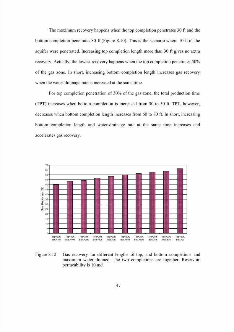
7/23/2019 Armenta Dis
http://slidepdf.com/reader/full/armenta-dis 165/263

7/23/2019 Armenta Dis
http://slidepdf.com/reader/full/armenta-dis 166/263
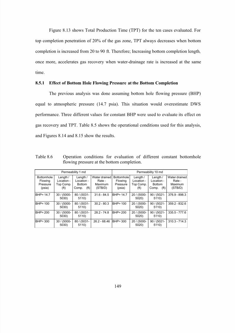
7/23/2019 Armenta Dis
http://slidepdf.com/reader/full/armenta-dis 167/263
Figure 8.13 shows Total Production Time (TPT) for the ten cases evaluated. For
top completion penetration of 20% of the gas zone, TPT always decreases when bottom
completion is increased from 20 to 90 ft. Therefore; Increasing bottom completion length,
once more, accelerates gas recovery when water-drainage rate is increased at the same
time.
8.5.1 Effect of Bottom Hole Flowing Pressure at the Bottom Completion
The previous analysis was done assuming bottom hole flowing pressure (BHP)
equal to atmospheric pressure (14.7 psia). This situation would overestimate DWS
performance. Three different values for constant BHP were used to evaluate its effect on
gas recovery and TPT. Table 8.5 shows the operational conditions used for this analysis,
and Figures 8.14 and 8.15 show the results.
Table 8.6 Operation conditions for evaluation of different constant bottomholeflowing pressure at the bottom completion.
Permeability 1 md Permeability 10 md
BottomholeFlowing
Pressure(psia)
Length /Location -
Top Comp.(ft)
Length /Location -
BottomComp. (ft)
Water drainedRate -
Maximum(STB/D)
BottomholeFlowing
Pressure(psia)
Length /Location -
Top Comp.(ft)
Length /Location -
BottomComp. (ft)
Water drainedRate -
Maximum(STB/D)
BHP= 14.7 30 / (5000-5030)
80 / (5031-5110)
31.6 - 84.5 BHP= 14.7 20 / (5000-5020)
90 / (5021-5110)
376.9 - 898.3
BHP= 100 30 / (5000-5030)
80 / (5031-5110)
30.2 - 80.3 BHP= 100 20 / (5000-5020)
90 / (5021-5110)
359.2 - 832.6
BHP= 200 30 / (5000-5030)
80 / (5031-5110)
28.2 - 74.8 BHP= 200 20 / (5000-5020)
90 / (5021-5110)
335.5 - 777.6
BHP= 300 30 / (5000-5030)
80 / (5031-5110)
26.2 - 68.46 BHP= 300 20 / (5000-5020)
90 / (5021-5110)
310.3 - 714.3
149

7/23/2019 Armenta Dis
http://slidepdf.com/reader/full/armenta-dis 168/263
BHP= 14.7
psiaBHP=100
psiaBHP=200
psia BHP=300
psia
k= 1 md
k= 10 md0
10
20
30
40
50
60
70
G a s R e c o v e r y ( % )
Figure 8.14 Gas recovery for different constant BHP at the bottom completion.
Figure 8.14 shows that increasing BHP at the bottom completion from 14.7 psia
to 300 psia slightly reduces gas recovery (gas recovery reduces from 64.37% to 62.1%
for permeability 1 md, and from 64.37% to 62.1% for permeability 10 md).
BHP= 14.7
psiaBHP=100
psiaBHP=200
psia BHP=300psia
0
10,000
20,000
30,000
40,000
50,000
60,000
T o t a l P r o d u c t i o n T i m e ( D a y s )
Permeability 1 md
BHP= 14.7
psiaBHP=100
psia
BHP=200
psia BHP=300psia
0
1,000
2,000
3,000
4,000
5,000
6,000
T o t a l P r o d u c t i o n T i m e ( D a y s )
Permeability 10 md
Figure 8.15 Total Production Time for evaluation of different constant BHP at the
bottom completion.
150

7/23/2019 Armenta Dis
http://slidepdf.com/reader/full/armenta-dis 169/263
Increasing BHP at the bottom completion from 14.7 psia to 300 psia increases
total production time, particularly for permeability 10 md (Figure 8.15). This is because
less amount of water is drained from the bottom completion when the bottomhole
pressure (BHP) is increased delaying well life. For permeability 1 md, however, the
situation reverses when BHP is increased beyond 100 psia. Increasing BHP at the bottom
completion from 100 psia to 200 psia reduces the amount of water drained increasing the
aquifer effect on the reservoir. Bottom hole pressure at the top completion is higher for
BHP=200 psia than for BHP=100 psia (Figure 8.16). Also, average reservoir pressure is
higher for BHP=200 psia than for BHP=100psia (Figure 8.17). In short, for permeability
1 md, increasing BHP at the bottom completion beyond 100 psia increases aquifer effect
on the reservoir pressure, reducing well life.
0
100
200
300
400
500
600
700
800
900
0 10000 20000 30000 40000 50000 60000
Time (Days)
B o t t o m h o l e F l o w i n g P r e s s u r
e ( p s i a
Top Completion (BHP= 200 psia) Bottom Completion (BHP= 200 psia)Top Completion (BHP= 100 psia) Bottom Completion (BHP= 100 psia)
Bottom Completion (BHP= 200 psia)
Bottom Completion (BHP= 100 psia)
TopCompletion (BHP= 100 psia)
TopCompletion (BHP= 200 psia)
Figure 8.16 Flowing Bottomhole Pressure history at the top, and bottom completion for
two different constant BHP at the bottom completion (100 psia, and 200 psia). Permeability is 1 md.
151

7/23/2019 Armenta Dis
http://slidepdf.com/reader/full/armenta-dis 170/263
0
200
400
600
800
1000
1200
0 10000 20000 30000 40000 50000 60000
Time (Days)
A v e r a g e R e s e r v o i r P r e s s u r e ( p s i a )
Reservoir Pressure (BHP= 200 psia) Reservoir Pressure (BHP= 100 psia)
Figure 8.17 Average reservoir for two different constant BHP at the bottom completion
(100 psia, and 200 psia). Permeability is 1 md.
Another important observation is that the BHP at the top and bottom completion
is always different (Figure 8.16). There is a drawdown of at least 150 psia (for BHP at the
bottom completion equal to 200 psia), and 250 psia (for BHP at the bottom completion
equal to 100 psia). It is not possible to have this drawdown for two close-completion
without isolation. Therefore, the packer insulation between the two completions is needed
for the DWS completion in low productivity gas wells to guarantee the drawdown
between the completions. This observation is in general agreement with the discussion
included on section 7.3.3 when DWS was compared with DGWS.
152

7/23/2019 Armenta Dis
http://slidepdf.com/reader/full/armenta-dis 171/263
8.6 When to Install DWS in Gas Wells
Four different scenarios for “when” DWS should be installed were evaluated:
when water production begins in a top short completion (30% for permeability 1 md and
20% for permeability 10 md), at late time in a totally perforated well, from day one of
production, and after the well die. Water-drainage is maximum all the time for the
scenarios when DWS is installed. The top completion length is 30 feet for permeability 1
md and 20 feet for permeability 10 md. The bottom completion length is 70 feet for
permeability 1 md and 80 feet for permeability 10 md. Table 8.7 includes the operation
conditions for the cases used for this study, and Figures 8.18 and 8.19 show the results.
Table 8.7 Operation conditions for “when” to install DWS in low productivity gas
well.
Permeability 1 md Permeability 10 md
Water DrainedRate
Length /Location -
Top Comp.(ft)
Length /Location -
BottomComp. (ft)
When InstallingDWS
Water DrainedRate
Length /Location -
Top Comp.(ft)
Length /Location -
BottomComp. (ft)
WhenInstalling
DWS
Qw = Max 30 (5000-5030)
70 (5031-5100)
After well died Qw = Max 20 / (5000-5020)
80 / (5021-5100)
After welldied
Qw = Max 30 (5000-5030)
70 (5031-5100)
Late time in atotally
perforated well
Qw = Max 20 / (5000-5020)
80 / (5021-5100)
Late time ina totally
perforatedwell
Qw = Max 30 (5000-5030)
70 (5031-5100)
Waterproduction startsin the top short
completion
Qw = Max 20 / (5000-5020)
80 / (5021-5100)
Waterproductionstarts in the
top shortcompletion
Qw = Max 30 (5000-5030) 70 (5031-5100) From day one Qw = Max 20 / (5000-5020) 80 / (5021-5100) From dayone
153

7/23/2019 Armenta Dis
http://slidepdf.com/reader/full/armenta-dis 172/263
After the
well dieLate in a
totally
Perforated
When
Water
Prod.
begins in a
30% Perf.
From Day
One After the
well dieLate in a
totally
Perforated
When
Water
Prod.
begins in a
20% Perf.
From Day
One
k = 1 md
k = 10 md
0
10
20
30
40
50
60
G a s R
e c o v e r y ( % )
Figure 8.18 Gas recovery for different times of installing DWS.
0
10,000
20,000
30,000
40,000
50,000
60,000
T o t a l P r o d u c t i o n T i m e ( D a y s )
After the well
die
Late in a
totally
Perforated
When Water
Prod. begins
in a 30%
Perf.
From Day
One
Permeability 1 md
0
1,000
2,000
3,000
4,000
5,000
6,000
T o t a l P r o d u c t i o n T i m e ( D a y s )
After the well
die
Late in a
totally
Perforated
When Water
Prod. begins
in a 30%
Perf.
From Day
One
Permeability 10 md
Figure 8.19 Total production time for different times of installing DWS.
154

7/23/2019 Armenta Dis
http://slidepdf.com/reader/full/armenta-dis 173/263
Figure 8.18 shows that: The lowest recovery occurs when DWS is installed after
the well die (Actually, there is no extra recovery when DWS is installed after the well
die); the highest recovery happens when DWS is installed from day one, and when water
production begins (The final recovery is almost the same when DWS is installed from
day one of production or at the beginning of water production in a short top perforated
well); Installing DWS late in a totally perforated well reduces final gas recovery.
Total production time slightly decreases when DWS is installed from day one
than when water production begins; Total production time is shorter when DWS is
installed late in a totally perforated well than when is installed from day one or when
water production begins (Figure 8.19).
Some comments can be made for DWS completion in a low productivity reservoir
from the previous analysis:
• DWS should not be installed after the well die. It is better to use another
technology available solving water production problems such as: gas lift,
pumping units, plunger, soap injection, etc.
• There is no extra benefit installing DWS from day one of well production.
• DWS should be installed early in the well life after water production begins.
Figure 8.20 shows the gas recovery history for the scenarios considered when
permeability is 10 md (the scenario “after the well died” is represented by the
conventional 100% perforated well because there is no extra gas recovery when DWS is
installed after the well has died). It is shown that the final gas recovery is the same when
DWS is installed from day one and when it is installed after water production begins.
155

7/23/2019 Armenta Dis
http://slidepdf.com/reader/full/armenta-dis 174/263
0
5
10
15
20
25
30
35
40
45
50
55
60
65
70
0 1000 2000 3000 4000 5000 6000
Time (Days)
G a s R e c o v e r y F a c t o r ( % )
Late in a Totally Perf. Conv. 100% Perf. When Water Prod. Begins in a 20% Perf. From Day One
Figure 8.20 Cumulative gas recovery for different times of installing DWS. Reservoir
permeability is 10 md.
8.7 Recommended DWS Operational Conditions in Gas Wells
According to this study, the best operational conditions for DWS in gas wells are:
• Water should be drained with the bottom completion at the highest rate
possible;
• The top completion should be short, penetrating between 20% to 40% of the
gas zone;
• The two completions should be as close as possible;
• A packer is needed to insolate the completions;
• The bottom completion should be long, penetrating the rest of the gas zone
and even the top of the aquifer;
• DWS should be installed early in the well life after water production begins.
156

7/23/2019 Armenta Dis
http://slidepdf.com/reader/full/armenta-dis 175/263
157
• Producing the drained-water at the surface together with the gas from the
bottom completion, instead of injecting the water downhole, has little effect
on the final gas recovery. Therefore, drained water can be lifted to the
surface when there is no deeper injection-zone.

7/23/2019 Armenta Dis
http://slidepdf.com/reader/full/armenta-dis 176/263
CHAPTER 9
CONCLUSIONS AND RECOMMENDATIONS
9.1 Conclusions
• In gas wells, a water cone is generated in the same way as in the oil-water system.
The shape at the top of the cone, however, is different in oil-water than in gas-
water systems. For the oil-water, the top of the cone is flat. For the gas-water
system, a small inverse gas cone is generated locally around the completion. This
inverse cone restricts water inflow to the completions. Also, the inverse gas cone
inhibits upward progress of the water cone.
• Vertical permeability, aquifer size, Non-Darcy flow effect, density of perforation,
and flow behind casing are unique mechanisms improving water
coning/production in gas reservoirs with bottom water drive.
• There is a particular pattern for water production rate at a gas well located in a
water drive reservoir with a channel in the cemented annuls—having a single
entrance at its end-. First, there is no water production. Next, water production
starts and water rate increases almost linearly. This increment is more dramatic
when the channel is originally in the water zone. Then, water rate stabilizes.
Finally, water rate increases exponentially. This pattern is explained because of
the flowing phases (single of two phase flow) in the channel at different
production steps of the well.
• Non-Darcy flow effect is important in low-rate gas wells producing from low-
porosity, low-permeability gas reservoirs. It is possible to have a gas well flowing
158
7/23/2019 Armenta Dis
http://slidepdf.com/reader/full/armenta-dis 177/263
at 1 MMscfd with 60% of the pressure drop generated by the Non-Darcy flow
effect (porosity 1%, permeability 1 md).
• Setting the Non-Darcy flow component at the wellbore does not make reservoir
simulators represent correctly the Non-Darcy flow effect in gas wells. Non-Darcy
flow should be considered globally (distributed throughout the reservoir) to
correctly predict the gas rate and recovery.
• Cumulative gas recovery could be reduced up to 42.2% when Non-Darcy flow
effect is considered throughout the reservoir in gas reservoirs with bottom water
drive. This is because the well loads up early and is killed for water production.
• The most promising design of Downhole Water Sink (DWS) installation in gas
wells includes dual completion with isolated packer between them and gravity
gas-water separation at the bottom completion. The design allows good control of
water coning outside the well and increases coning of gas and maximum rate at
the top completion with no water loading.
• The highest recovery for a conventional gas well in the low-permeability reservoir
(1-10 md) occurs when the gas zone is totally penetrated. For permeability 100
md, gas recovery becomes almost insensitive to the completion length for
penetration greater than 30%.
• Gas recovery increases with permeability for a gas reservoir with bottom water
drive. In general, high permeability allows higher gas rates with smaller reservoir
drawdown; therefore the well has more energy to produce gas with higher water
cut.
159

7/23/2019 Armenta Dis
http://slidepdf.com/reader/full/armenta-dis 178/263
7/23/2019 Armenta Dis
http://slidepdf.com/reader/full/armenta-dis 179/263
would be installed early at the well life after water production begins. Producing
the drained-water at the surface together with the gas from the bottom completion,
instead of injecting the water downhole, has little effect on the final gas recovery.
9.2 Recommendations
• The water rate pattern found in a gas well with leaking cement could be
confirmed using field data. Production data for gas wells with leaking cement
would be analyzed looking for the described pattern.
• Effects of Non-Darcy flow in low-productivity gas wells should be studied
considering a fracture in the well. A normal practice in the industry is to fracture
gas wells with low productivity. Non-Darcy flow distributed in the reservoir and
into the fracture should be considered.
• Effects of a fracture and permeability heterogeneity in water production, and final
gas recovery should be evaluated in water drive gas reservoirs using numerical
simulators.
• More possible configurations for DWS in gas wells should be evaluated. A single
very long completion (totally perforating the gas zone and the top of the aquifer)
without a packer could be one of the many new possibilities.
• Economic evaluation of DWS in gas wells should be done. This evaluation should
consider not only injecting drained-water into a lower zone but lifting water to the
surface, also.
• A combined mechanism of DWS and two fractures (one in the top completion and
the other in the bottom completion) in a low productivity gas well should be
evaluated.
161

7/23/2019 Armenta Dis
http://slidepdf.com/reader/full/armenta-dis 180/263
162
• More in-depth study involving different modeling, reservoir properties, and
production conditions should be done getting a better understanding of DWS
operations in gas reservoir.
• More in-depth study involving different modeling, reservoir properties, and
production conditions should be done for comparison of DWS and DGWS
identifying best opportunity for each technology.
• A field pilot project installing DWS in low productivity gas reservoirs should be
conducted. This project should refine the operational optimization performed in
this research, giving new information about the possibilities of DWS in low
productivity gas reservoirs.

7/23/2019 Armenta Dis
http://slidepdf.com/reader/full/armenta-dis 181/263
REFERENCES
Abercrombie, B., 1980, “Plunger Lift,” The Technology of Artificial Lift Methods,” Vol.
2b, K.E. Brown (ed), PennWell Publ. Co., Tulsa, OK (1980), p483-518.
Adams, L.S., and Marsili, D.L., 1992, “Design and Installation of a 20,500-ft Coiled
Tubing Velocity String in the Gomez Field, Pecos County, Texas,” paper SPE
24792, 67 th
Annual Technical Conference and Exhibition, Washington, D.C.,October 4-7.
Agarwal, R.G., Al-Hussainy, R., and Ramey, Jr. H.J., 1965, “The Importance of WaterInflux in Gas Reservoir,” Journal of Petroleum Technology, November, 1965,
p1336-42.
Aguilera, R., Conti, J.J., Lagrenade E., 2002, “Reducing Gas Production Decline
Through Dewatering: A Case History From the Naturally Fractured AguaragueField, Salta, Argentina,” paper SPE 75512, SPE Gas Technology Symposium,
Calgary, Canada, 30 April-2 May.
Alvarez, C.H., Holditch, S.A, McVay, D.A., 2002, “Effects of Non-Darcy Flow on
Pressure Transient Analysis of Hydraulically Fractured Gas Wells,” paper SPE77468, Annual Technical Conference and Exhibition, San Antonio, TX, 29
September-2 October.
Amyx, J.W., Bass, D.M., Whitinig, R.L. 1960, “Petroleum Reservoir Engineering,”
McGraw-Hill , New York, p 64-68.
Arcaro, D. P. and Bassiouni, Z. A., 1987, “The Technical And Economic Feasibility of
Enhanced Gas Recovery in The Eugene Island Field by Use a CoproductionTechnique,” Journal of Petroleum Technology (May 1987), p585-90.
Armenta, M., and Wojtanowicz, A.K., 2003, “Incremental Recovery Using Dual-
Completed Wells in Gas Reservoir with Bottom Water Drive: A FeasibilityStudy,” paper 2003-194 Canadian International Petroleum Conference-2003,
Calgary, Alberta, Canada, June 10-12.
Armenta, M., White, C., Wojtanowicz, A.K., 2003, “Completion Length Optimization in
Gas Wells,” paper 2003-192 Canadian International Petroleum Conference-2003,
Calgary, Alberta, Canada, June 10-12.
Armenta, M., and Wojtanowicz, A., 2002, “Severity of Water Coning in Gas Wells,”
paper SPE 75720 SPE Gas Technology Symposium, Calgary, Alberta, Canada, 30April-2 May.
Arthur, M.G., 1944, “Fingering and Coning of Water and Gas in Homogeneous Oil
Sand,” AIME Transactions, Vol. 155, 184-199.
163

7/23/2019 Armenta Dis
http://slidepdf.com/reader/full/armenta-dis 182/263
Avery, D.J. and Evans, R.D., 1988, “Design Optimization of Plunger Lift Systems,”
paper SPE 17585, International Meeting on Petroleum Engineering of the SPE ,Tianjin, China, Nov. 1-4.
Awadzi, J., Babbitt, J., Holland, S., Snyder, K., Soucer, T., Latter, K., 1999, “Downhole
Capillary Soap Injection Improves Production,” paper SPE 52153, Mid-ContinentOperations Symposium, Oklahoma City, OK, March 28-31.
Baruzzi, J.O.A., Alhanati, F.J.S., 1995, “Optimum Plunger Lift Operation,” paper SPE29455, Production Operations Symposium, Oklahoma City, OK, April 2-4.
Bear, J., 1972, “Dynamic of Fluids in Porous Media”, Dover Publications, INC., NewYork.
Beauregard, E., and Ferguson, P.L., 1982, “Introduction to Plunger Lift: Applications,Advantages and Limitations,” paper SPE 10882, Rocky Mountain Regional
Meeting of the SPE , Billings, MT, May 19-21.
Beattle, D.R. and Roberts, B.E., 1996, “Water Coning in Naturally Fractured GasReservoirs,” Paper SPE 35643, Gas Technology Conference, Calgary, Alberta,
Canada, 28 April – 1 May.
Beeson, C.M., Knox, D.G., and Stoddard, J.H., 1958, “Short-Cut Design Calculations and
Field Applications of the Plunger Lift Method of Oil Production,” The Petroleum
Engineer , (June-Oct. 1958).
Beggs H.D. 1984, “Gas Production Operation,” Oil and Gas Consultants International ,Inc, Tulsa, Oklahoma, p53-59.
Berry, D. A., 196, “Statistics: A Bayesian Perspective,” Wadsworth Publishing Co., Belmont, CA, 518 p.
Bizanti, M.S., and Moonesan, A., 1989, “How to Determine Minimum Flow Rate for
Liquid Removal,” World Oil, (September, 1989), p 71-73.
Bourgoyne, A.T., Chenevert, M.E., Millheim, K.K., Young, F.S. 1991, “Applied Drilling
Engineering,” Society of Petroleum Engineering Textbook Series Volume 2,Richardson, TX, p137-155.
Box, G. E. P. and Cox D.R., 1964 “An Analysis of Transformations,” J. of the RoyalStatistical Society, 26 No. 2, 211-252
Box, G. E. P. and Tidwell, P.W., 1962 “Transformation of the Independent Variables,”
Technometrics, 4 No. x, 531-550.
Brady, C.L., and Morrow, S.J., 1994, “An Economic Assessment of Artificial Lift in
Low-Pressure Tight Gas Sands in Ochiltree County, Texas,” paper SPE 27932,SPE Mid-Continent Gas Symposium, Amarillo, TX, May 22-24.
164
7/23/2019 Armenta Dis
http://slidepdf.com/reader/full/armenta-dis 183/263
Brar, S.G., Aziz, K., 1978, “Analysis of Modified Isochronal Test To Predict TheStabilized Deliverability Potential of Gas Well Without Using Stabilized Flow
Data,” JPT (Feb.) 297-304; Trans. AIME , p297-304.
Campbell, S., Ramachandran, S., and Bartrip, K., 2001, “Corrosion Inhibition/FoamerCombination Treatment to Enhance Gas Production,” paper SPE 67325,
Production and Operations Symposium, Oklahoma City, OK, March 24-27.
Chaperon, I., 1986, “Theoretical Study of Coning Toward Horizontal and Vertical Wells
in Anisotropic Formations: Subcritical and Critical Rates,” paper SPE 15377, SPE
Annual Technical Conference and Exhibition, New Orleans, Oct. 5-8.
Cohen, M.F. 1989, “Recovery Optimization in a Bottom/Edge Water-Drive Gas
Reservoir, Soehlingen Schneverdinge,” paper SPE 19068 SPE Gas TechnologySymposium, Dallas, June 7-9.
Coleman, S.B., Hartley, B.C., McCurdy, D.G., and Norris III, H.L., 1991, “A New Look
at Predicting Gas-Well Load-up,” J. Pet. Tech. (Mar. 1991) p329-38.
Computer Modelling Group Ltda, 2001, “User’s Guide, IMEX, Advanced Oil/Gas
Reservoir Simulator,” CMG, p425-26.
Craft B.C. and Hawkins M.F. 1959, “Applied Petroleum Reservoir Engineering,”
Prentice Hall PTR, Englewood Cliffs, NJ, p300-01.
Craft B.C. and Hawkins M.F. 1991, “Applied Petroleum Reservoir Engineering,” Prentice Hall PTR, Englewood Cliffs, NJ, p226-227; 280-299.
Dake L.P., 1978, “Fundamentals of Reservoir Engineering,” Elsevier Scientific Publishing Company, New York, p255-258.
Damsleth, E., Hage, A. and Volden, R., 1992: “Maximum Information at Minimum Cost:
A North Sea Field Development Study with Experimental Design,” J. Pet. Tech (December 1992) 1350-1360.
Dejean, J.-P., and Blanc, G., 1999, “Managing Uncertainties on Production PredictionsUsing Integrated Statistical Methods,” Paper SPE 56696, SPE Annual Technical
Conference and Exhibition, Houston, Texas, 3-6 October.
Dranchuck, P.M., Purvis, R.A., and Robinson, D.B., 1974, “Computer Calculations of
Natural Compressibility Factors Using the Standing and Katz Correlations,”
Institute of Petroleum Technical Series.
Economides, M.J., Oligney, R.E., Demarchos, A.S., and Lewis, P.E., 2001, “Natural Gas:
Beyond All Expectations,” Paper SPE 71512, Annual Technical Conference and
Exhibition, New Orleans, 30 September- 3 October.
165

7/23/2019 Armenta Dis
http://slidepdf.com/reader/full/armenta-dis 184/263
E&P Environment, 2001, “GTI Studies Gas Well Water Management,” J&E
Communication, Inc, Vol. 12 No. 23, p1-4.
Elmer, W.G., 1995, “Tubing Flow Rate Controller: Maximize Gas Well Production From
Start To Finish,” paper SPE 30680, SPE Annual Technical Conference and
Exhibition, Dallas, September 22-25.
Energy Information Administration, 2000, “Distribution of Gas Wells and Production,”
http://www.eia.doe.gov/pub/poi_gas/petrosystem/natural_gas/petrosysgas.html
Energy Information Administration, 2001, “U.S. Crude Oil, Natural Gas, and Natural Gas
Liquids Reserves 2001 Annual Report,”http://www.eia.doe.gov/pub/oil_gas/natural_gas/data_publications/crude_oil_natu
ral_gas_reserves/current/pdf/ch4.pdf
Energy Information Administration, 2001, “U.S. Natural Gas Markets: Recent Trends
and Prospects For the Future,”http://tonto.eia.doe.gov/FTPROOT/service/oiaf0102.pdf
Energy Information Administration, 2003, “Annual Energy Outlook 2003 With
Projection to 2025,” www.eia.doe.gov/oiaf/aeo, January.
Energy Resources and Conservation Board , 1975, Theory and Practice of The Testing of
Gas Wells, third edition, Pub. ERCB-75-34, ERCB, Calgary, Alberta, p3-18 to p3-
21.
Ergun, S. and Orning, A.A., 1949, “Fluid Flow Through Ramdomly Packed Collumnsand Fluidized Beds.” Industrial and Engineering Chemistry 41, No 6, p1179-
1184.
Evan, R.D., Hudson, C.S., Greenlee, J.E., 1987, “The Effect of an Immobile Liquid
Saturation on the Non-Darcy Flow Coefficient in Porous Media,” SPE Production
Engineering (November ), p331-38.
Ferguson, P.L., and Beauregard, E., 1985, “How to Tell if Plunger Lift Will Work in
Your Well,” World Oil , August 1, p33-36.
Fligelman, H., Cinco-Ley, H., Ramley Jr., Braester, C., Couri, F., 1989, “Pressure-
Drawdown Test Analysis of a Gas Well Application of New Correlation,” paper
SPE 17551 Facilities Engineering , September (1989) p409.
Flowers, J.R., Hupp, M.T., and Ryan, J.D., 2003, “The Results of Increased Fracture
Conductivity on Well Performance in a Mature East Texas Gas Field,” paper SPE84307 Annual Technical Conference and Exhibition, Denver, Colorado, October
5-8.
166

7/23/2019 Armenta Dis
http://slidepdf.com/reader/full/armenta-dis 185/263
Foss, D.L., and Gaul, R.B., 1965, “Plunger-Lift Performance Criteria with Operating
Experience-Ventura Avenue Field,” Drilling and Production Practice, API(1965), p124-40.
Frederick, D.C., Graves, R.M., 1994, “New Correlations To Predict Non-Darcy Flow
Coefficients at Immobile and Mobile Water Saturation,” paper SPE 28451 AnnualTechnical Conference and Exhibition, New Orleans, Sept. 25-28
Gasbarri, S. and Wiggins, M.L., 2002, “A Dynamic Plunger Lift Model for Gas Wells,”SPE Production and Facilities, May 2001, p89-96.
Geertsma, J., 1974, “Estimating the Coefficient of Inertial Resistance in Fluid Flowthrough Porous Media,” SPEJ (Oct. 1974) p445-450.
Girardi, F., Lagrenade, E., Mendoza, E., Marin, H. and Conti, J.J., 2001, “Improvementof Gas Recovery Factor Through the Application of Dewatering Methodology in
the Huamampampa Sands of the Agurague Field,” paper SPE 69565, SPE Latin American and Caribbean Petroleum Engineering Conference, Buenos Aires,
Argentina, March 25-28.
Golan M. and Whitson C., 1991, “Well Performance,” Prentice-Hall Inc., New Jersey,
p268-284.
Grubb, A.D., and Duvall, D.K., 1992, “Disposal Tool Technology Extends Gas Well Life
and Enhances Profits,” paper SPE 24796, 67th Annual Technical Conference and Exhibition of the SPE , Washington, D.C., October 4-7.
Hacksma, J.D., 1972, “Users Guide to Predict Plunger Lift Performance,” Proceeding,
Texas Tech. U. Southwestern Petroleum Short Course, Lubbock, TX.
Hasan, A.R., and Kabir, C.S., 1985, “Determining Bottomhole Pressures in Pumping
Wells,” SPEJ (Dec., 1985) 823-38.
Hebert, D.W., 1989, “A Systematic Approach To Design of Rod Pumps in CoalDegasification Wells: San Juan Basin, New Mexico,” paper SPE 19011, SPE
Joint Rocky Mountain Regional/Low Permeability Reservoirs Symposium and
Exhibition, Denver, Colorado, March 6-8.
Henderson L.J., 1984, “Deep Sucker Rod Pumping for Gas Well Unloading,” paper SPE
13199, 59th Annual Technical Conference and Exhibition, Houston, TX,September 16-19.
Hernandez, A., Marcano, L., Caicedo, S., and Carbunaru, R., 1993, “Liquid Fall-backMeasurements in Intermittent Gas Lift with Plunger,” paper SPE 26556, SPE Annual Technical Conference and Exhibition, Houston, TX, October 3-6.
167
7/23/2019 Armenta Dis
http://slidepdf.com/reader/full/armenta-dis 186/263
Hoyland, L.A., Papatzacos, P., and Skjaeveland, S.M., 1989, “Critical Rate for Water
Coning: Correlation and Analytical Solution,” SPE Reservoir Engineering, p459-502, November 1989.
Houpeurt, A., 1959, “On the Flow of Gases in Porous Media,” Revue de L’Institut
Français du Pétrole (1959)XIV
(11
), p1468-1684.
Hutlas, E.J. and Granberry, W.R., 1972, “A Practical Approach to Removing Gas Well
Liquids,” J. Pet. Tech., (August 1972) 916-22.
Ikoku, C.I., 1984, “Natural Gas Production Engineering,” John Wiley & Sons, New York,
p369.
Inikori, S.O., 2002, “Numerical Study of Water Coning Control With Downhole Water
Sink (DWS) Well Completions in Vertical and Horizontal Well,” PhDdissertation, Louisiana State University and A&M College, Baton Rouge, LA,
August.
Irmay, S, 1958, “On the Theoretical Derivation of Darcy and Forchheimer Formulas,”Trans., American Geophysical Union 39, No 4, p702-707.
Janicek, J.D., and Katz, D.L., 1995, “Applications of Unsteady State Gas FlowCalculations,” Proc., U. of Michigan Research Conference, June 20.
Jensen, J.L., Lake, L.W., Corbett, P.W.M., and Goggin, D.J., 2000, “Statistics forPetroleum Engineers and Geoscientists,” Elsevier , New York.
Jones, S.C., 1987, “Using the Inertial Coefficient, β, To Characterize Heterogeneity inReservoir Rock,” paper SPE 16949 SPE Annual Technical Conference and Exhibition, Dallas, Sept. 27-30.
Jones, L.G. and Watts, J.W., Feb. 1971, “Estimating Skin Effects in a PartiallyCompleted Damaged Well,” JPT 249-52; AIME Transactions, 251.
Joshi, S.D., 1991, “Horizontal Well Technology,” PennWell Books, Tulsa, Oklahoma,
p251-267.
Katz, D.L., Cornell, D., Kobayashi, R., Poettman, F.H., Vary, J.A., Elenbans, J.R., and
Weinaug, C.F., 1959, “Handbook of Natural Gas Engineering,” McGraw-Hill Book Co., Inc., New York, p46-51.
Kabir, C.S., 1983, “Predicting Gas Well Performance Coning Water in Bottom-WaterDrive Reservoirs,” Paper SPE 12068, 58
th Annual Technical Conference and
Exhibition, San Francisco, Oct 5-8.
Klein, S.T., 1991, “The Progressing Cavity Pump in Coaled Methane Extraction,” paperSPE 23454, SPE Eastern Regional Meeting , Lexington, Kentucky, October 22-25.
168

7/23/2019 Armenta Dis
http://slidepdf.com/reader/full/armenta-dis 187/263
Klein, S.T., Thompson, S., 1992, “Field Study: Utilizing a Progressing Cavity Pump for aClosed-Loop Downhole Injection System,” paper SPE 24795, 67
th Annual
Technical Conference and Exhibition of the SPE , Washington, D.C. October 4-7.
Lea, J.F., 1982, “Dynamic Analysis of Plunger Lift Operations,” Journal of PetroleumTechnology, (Nov. 1982), p2617-2629.
Lea, J.F., Winkler, H.W., and Snyder, R.E., 2003, “What’s new in artificial lift,” WorldOil, (April, 2003), p 59-75.
Lea Jr., J.F., and Tighe, R.E., 1983, “Gas Well Operation With Liquid Production,” PaperSPE 11583, Production Operation Symposium, Oklahoma City, OK, February 27-
March 1.
Lee J., 1982, Well Testing, Society of Petroleum Engineering of AIME Textbook Series
Volume 1, New York, p82-84.
Lee, A.L., Gonzales, M.H., and Eakin, B.E., 1966, “The Viscosity of Natural Gases,” Journal of Petroleum Technology, (August 1966).
Lee J. and Wattenbarger R. 1996, “Gas Reservoir Engineering”, Society of Petroleum Engineering Textbook Series Volume 5, Richardson, Texas, p32; p170-174;
p245.
Libson, T.N., Henry, J.R., 1980, “Case Histories: Identification of and Remedial Action
for Liquid Loading in Gas Wells –Intermediate Shelf Gas Play,” Journal of Petroleum Technology, (April, 1980), p685-93.
Liu, X., Civan, F., and Evans, R.D., 1995, “Correlation of the Non-Darcy FlowCoefficient,” J. Cdn. Pet. Tech. (Dec. 1995) 34, No 10, p50-54.
Lombard, J-M., Longeron, D., Kalaydjan, F., 1999, “Influence of Connate Water and
Condensate Saturation on Inertia Effect in Gas Condensate Fields,” paper SPE56485 SPE Annual Technical Conference and Exhibition, Houston, October 3-6.
Manceau, E., Mezghani M., Zabalza-Mezghani, I., and Roggero, F., 2001, “Combinationof Experimental Design and Joint Modeling Methods for Quantifying the Risk
Associated with Deterministic and Stochastic Uncertainties—An Integrated Test
Study,” paper SPE 71620, SPE Annual Technical Conference and Exhibition, New Orleans, Louisiana, 30 September-3 October.
Maggard, J.B., Wattenbarger, R.A., and Scott, S.L., 2000, “Modeling Plunger Lift forWater Removal From Tight Gas Wells,” paper SPE 59747, SPE/CERI GasTechnology Symposium, Calgary, Alberta Canada, April 3-5.
169

7/23/2019 Armenta Dis
http://slidepdf.com/reader/full/armenta-dis 188/263
Marcano, L. and Chacin, J., 1992, “Mechanistic Design of Conventional Plunger Lift
Installations,” paper SPE 23682, Second Latin American Petroleum EngineeringConference of the SPE , Caracas, Venezuela, March 8-11.
McLeod, H.D. Jr. Jan. 1983, “The Effect of Perforating Conditions on Well
Performance,” JPT, p31-39.
McMullan, J.H., Bassiouni, Z., 2000, “Optimization of Gas-Well Completion and
Production Practices,” Paper SPE 58983, International Petroleum Conference and Exhibition, Mexico, Feb 1-3.
Melton, C.G., and Cook, R.L., 1964, “Water-Lift and Disposal Operations in Low-Pressure Shallow Gas Wells,” Journal of Petroleum Technology (June 1964),
p619-22.
Meyer, H.I. and Garder, A.O., 1954, “Mechanics of Two Immiscible Fluids in Porous
Media,” Journal of Applied Physics, (November 1954)25
, No. 11, 1400.
Mills, R.A.R., Gaymard, R., 1996, “New Application for Wellbore Progressing CavityPumps,” paper SPE 35541, Intl. Petroleum Conference & Exhibition of Mexico,
Villahermosa, Mexico, March 5-7.
Montgomery, D.C., 1997, “Design and Analysis of Experiments,” 4th
ed., John Wiley and
Sons, Inc., New York City.
Mower, L.N., Lea, J.F., Beauregard, E., and Ferguson, P. L., 1985, “Defining the
Characteristics and Performance of Gas Lift Plungers,” paper SPE 14344, SPE Annual Technical Conference and Exhibition, Las Vegas, NV, Sept. 22-25.
Muskat, M.,1982, “Flow of Homogeneous Fluids,” International Human Resources Development , Boston, p687-692.
Muskat, M. and Wyckoff, R.D., 1935, “An approximate Theory of Water Coning in Oil
Production,” AIME Transactions, Vol. 114, 144-163.
Myers, R. H. and Montgomery, D. C., 2002, “Response Surface Methodology: Process
and Product optimization Using Designed Experiments,” 2nd
ed., John Wiley &Sons, New York.
National Energy Board of Canada, 1995, “Unconnected Gas Supply Study: Phase I –Evaluation of Unconnected Reserves in Alberta,” NEB Energy Resources Branch,
January.
Neves, T.R., and Brimhall, R.M., 1989, “Elimination of Liquid Loading in Low-
Productivity Gas Wells,” paper SPE 18833, SPE Production Operation
Symposium, Oklahoma City, OK, March 13-14.
170

7/23/2019 Armenta Dis
http://slidepdf.com/reader/full/armenta-dis 189/263
Nichol, J.R., and Marsh, J., 1997, “Downhole Gas/Water Separation: Engineering
Assessment and Field Experience,” paper SPE 38828, SPE Annual TechnicalConference and Exhibition, San Antonio, TX, October 5-8.
Nosseir, M.A., Darwich, T.A., Sayyouh, M.H., and El Sallaly, M., 2000, “a New
Approach for Accurate Prediction of Loading in Gas Wells Under DifferentFlowing Conditions,” SPE Prod. & Facilities 15 (4), November, p241-46.
Pascal H., Quillian, R.G., Kingston, J., 1980, “Analysis of Vertical Fracture Length and Non-Darcy Flow Coefficient Using Variable Rate Tests,” paper SPE 9438 Annual
Technical Conference and Exhibition, Dallas, Sept. 21-24.
Petalas, N & Aziz, K, 1997, “A Mechanistic Model for Stabilized Multiphase Flow in
Pipe,” Petroleum Engineering Department, Stanford University, August 1997.
Pigott, M.J., Parker, M.H., Mazzanti, D.V., Dalrymple, L.V., Cox, D.C., and Coyle, R.A.,
2002, “Wellbore Heating To Prevent Liquid Loading,” paper SPE 77649, SPE Annual Technical Conference and Exhibition, San Antonio, TX, 29 September-2
October.
Putra, S.A., and Christiansen R.L., 2001, “Design of Tubing Collar Inserts for Producing
Gas Wells Bellow Their Critical Rate,” paper SPE 71554, SPE Annual TechnicalConference and Exhibition, New Orleans, Louisiana, September 30- October 3.
R Core Team, 2000, “The R Reference Index: Version 1.1.1.”
Rangel-German, E., and Samaniego V., F, 2000, “On the determination of the skin factorand the turbulence term coefficient through a single constant gas pressure test,” J.
of Pet. Sci. & Eng., (2000) 26, p121.
Randolph, P.L., Hayden, C.G., and Anhaiser, J.L., 1991, “Maximizing Gas Recovery
From Strong Water Drive Reservoir,” paper SPE 21486, SPE Gas Technology
Symposium, Houston, TX, January 23-25.
Rogers, L.A., 1984, “Test of Secondary Gas Recovery by Coproduction of Gas and
Water From Mt. Selman Field, TX,” paper SPE 12865, SPE/DOE/GRI
Unconventional Gas Recovery Symposium, Pittsburgh, PA, May 13-15.
Roman, S., 1999, “Writing Excel Macros,” O'Reilly and Associates, Sebastopol,
California, p529.
Rosina, L, 1983, “A Study of Plunger Lift Dynamics,” MS Thesis, The University of
Tulsa, Tulsa, OK.
Rudolph J., and Miller J., 2001 “Downhole Produced Water Disposal Improves Gas
Rate,” GasTIPS, pp 21-24, Fall 2001.
171

7/23/2019 Armenta Dis
http://slidepdf.com/reader/full/armenta-dis 190/263
Sacks, J., S. B. Schiller, and W. J. Welch, 1989, “Designs for Computer Experiments,”
Technometrics (1989) 31 No. 1, 41-47.
Saidikowski, R.M., 1979, “Numerical Simulations of the Combined Effects of Wellbore
Damage and Partial Penetration,” Paper SPE 8204 Annual Fall Technical
Conference and Exhibition, Nevada, Sep 23-26.
Saleh, S., and Al-Jamae’y, M., 1997, “Foam-Assisted Liquid Lifting in Low Pressure Gas
Wells,” paper SPE 37425, Production Operations Symposium, Oklahoma City,Marc 9-11.
Scheidegger, A.E., 1974, “The Physics of Flow through Porous Media,” University ofToronto Press, Toronto.
Schlumberger: VFPi User Guide 98A, 1998, Sclumberger GeoQuest , App. N, pN-1 to N-8.
Schlumberger Technology Co., 1997, Eclipse 100 Reference Manual, Sclumberger
GeoQuest , unpaginated.
Schneider, T.S., and Mackey, Jr. V., 2000, “Plunger Lift Beneficts Bottom Line for a
Southeast New Mexico Operator,” paper SPE 59705, SPE Permian Basin Oil andGas Recovery Conference, Midland, TX, March 21-23.
Schols, R.S., 1972, “An Empirical Formula for the Critical Oil Production Rate,” Erdoel Erdgas, Z, Vol 88, No 1, p6-11, January 1972.
Schwall, G.H., 1989, “Case Histories: Plunger Lift Boosts Production in Deep
Appalachian Gas Wells,” paper SPE 18870, SPE Production Operations
Symposium, Oklahoma City, OK, March 13-14.
Scott, W.S., and Hoffman, C.E., 1999, “An Update On Use of Coiled Tubing for
Completion and Recompletion Strings,” paper SPE 57447, SPE Eastern Regional
Meeting , Charleston, West Virginia, October 21-22.
Shirman, E.I., Wojtanowicz, A.K., 1997, “Water Coning Reversal Using Downhole
Water Sink Theory and Experimental Study,” paper SPE 38792, SPE AnnualTechnical Conference & Exhibition, San Antonio, TX, Oct.
Shirman, E.I., Wojtanowicz, A.K., 1998 “More Oil With Less Water Using DownholeWater Sink Technology: A Feasibility Study,” paper SPE 49052 73
rd SPE Annual
Technical Conference & Exhibition, New Orleans, LA, Oct. 27-30.
Silverman, S.A., Butler, W., Ashby, T., and Snider, K., 1997, “Concentric Capillary
Tubing Boosts Production of Low-Pressure Gas Wells,” Hart’s Petroleum
Engineer International, Vol. 70, No 10, October 1997, p71-73.
172

7/23/2019 Armenta Dis
http://slidepdf.com/reader/full/armenta-dis 191/263
Smith, R.V., 1990, “Practical Natural Gas Engineering,” 2nd
Edition, PennWell Books,
Tulsa, 1990.
Stephenson G.B., Rouen R.P., Rosenzweig M.H., 2000, “Gas-Well Dewatering: A
Coordinated Approach,” paper SPE 58984, 2000 SEP International Petroleum
Conference and Exibition, Villahermosa, Mexico, February 1-3.
Sutton, R.P., Cox, S. A., Williams Jr., E. G., Stoltz, R.P., and Gilbert, J.V., 2003, “Gas
Well Performance at Subcritical Rates,” paper SPE 80887, SPE Production andOperations Symposium, Oklahoma City, OK, March 22-25.
Swisher, M.D. and Wojtanowicz, A.K., 1995, “In Situ-Segregated Production of Oil andWater – A Production Method with Environmental Merit: Field Application,”
paper SPE 29693 SPE/EPA Exploration & Production Environmental
Conference, Houston, TX, March 27-29.
Swisher, M.D. and Wojtanowicz, A.K., 1995, “New Dual Completion Method EliminatesBottom Water Coning,” paper SPE 30697, SPE Annual Technical Conference &
Exhibition, Dallas, TX, Oct. 22-25.
Thauvin, F., and Mohanty, K.K., 1998, “Network Modeling of Non-Darcy Flow through
Porous Media,” Transport in Porous Media, 31, p19-37.
Timble, A.E., DeRose, W.E., 1976, “Field Application of Water-Conning Theory to
Todhunters Lake Gas Field,” Paper SPE 5873, SPE-AIME 46 th
Annual California Regional Meeting , Long Beach, April 8-9.
Tiss, M. and Evans, R.D., 1989, “Measurement and Correlation of Non-Darcy Flow
Coefficient in Consolidated Porous Media,” J. Petroleum Science and
Engineering , Vol. 3, Nos. 1-2, p19-33.
Turner, R.G, Hubbard, M.G., and Dukler, A.E., 1969, “Analysis and Prediction of
Minimum Flow Rates for the Continuous Removal of Liquid from Gas Wells,” J.
Pet. Tech. (Nov., 1969) 1475-82.
Umnuayponwiwat, S., Ozkan, E., Pearson, C.M., and Vincent, M., 2000, “Effect of non-
Darcy flow on the interpretation of transient pressure responses of hydraulicallyfractured wells,” paper SPE 63176 presented at the SPE Annual Technical
Conference and Exhibition, Dallas, October 1-4.
Upchurch, E.R., 1987, “Expanding the Range for Predicting Critical Flowrates of Gas
Well Producing From Normally Pressured Water Drive Reservoir,” paper SPE
16906, SPE Annual Technical Conference and Exhibition, Dallas, September 27-30.
Vosika, J.L., 1983, “Use of Foaming Agents to Alleviate Loading in Great Green River
TFG Wells,” paper SPE/DOE 11644, SPE/DOE Symposium on Low Permeability, Denver, Colorado, March 14-16.
173

7/23/2019 Armenta Dis
http://slidepdf.com/reader/full/armenta-dis 192/263
174
Weeks, S., 1982, “Small-Diameter Concentric Tubing Extends Economic Life of HighWater/Sour Gas Edwards Producers,” Journal of Petroleum Technology,
(September, 1982), p1947-50.
White, C., 2002, “PETE-4052 Well Testing,” Syllabus, Louisiana State University, Craft& Hawkins Petroleum Engineering Department.
White, G.W., 1982, “Combine Gas Lift, Plunger to Increase Production Rate,” World Oil (Nov. 1982), p69-74.
White, C.D., and Royer, S.A., 2003, “Experimental Design as a Framework for ReservoirStudies,” paper SPE 79676, SPE Reservoir Simulation Symposium, Houston,
February 3-5.
White, C.D., Willis, B.J., Narayanan, K., and Dutton, S.P., 2001, “Identifying and
Estimating Significant Geologic Parameters with Experimental Design,” SPEJ (September 2001) 311-324.
Wiggins, M. L., Nguyen, S.H., and Gasbarri, S., 1999, “Optimizing Plunger Lift
Operations in Oil and Gas Wells,” paper SPE 52119, SPE Mid-Continent
Operations Symposium, Oklahoma City, Oklahoma, March 28-31.
Wojtanowicz, A.K., Shirman, E.I., Kurban, H., 1999, “Downhole Water Sink (DWS)
Completion Enhance Oil Recovery in Reservoir With Water Coning Problems,” paper SPE 56721, SPE Annual Technical Conference & Exhibition, Houston, TX,
Oct. 3-6.
Xu, R., Yang, L., 1995, “A New Binary Surfactant Mixture Improved Foam Performance
in Gas Well Production,” paper SPE 29004, International Symposium on OilfieldChemistry, San Antonio, TX, February 14-17.

7/23/2019 Armenta Dis
http://slidepdf.com/reader/full/armenta-dis 193/263
APPENDIX A
ANALYTICAL COMPARISON OF WATER CONING IN OIL AND GAS WELLS
1. Analytical comparison of water coning in oil and gas wells before waterbreakthrough
The pressure drop to generate a stable cone height of 20 feet in the oil-water
system is:
psi P
P
h P ow
2
20*)6.65.8(052.0
)(052.0
=∆
−=∆
−=∆ ρ ρ
The oil production rate for this pressure drop assuming pseudo-steady-state
conditions is:
])/472.0[ln(*
)(*00708.0 1
S r r B
p phk q
weo
eoo
+
−=µ
Assuming that the skin effect (S) is generated only by the partial penetration (skin
effects generated by drilling mud and perforation geometry are zero). After Saidikowski
(1979), S can be estimated from the equation:
−
−= 2ln1
V
H
w
t
p
t
k
k
r
h
h
hS
Where: ht is the reservoir thickness, h p is the completed interval, r w is the wellbore
radius, k H is the horizontal permeability, and k V is the vertical permeability.
For this example: 9.325.0
50ln1
20
50=
−
−=S
The oil flow rate is:
175

7/23/2019 Armenta Dis
http://slidepdf.com/reader/full/armenta-dis 194/263
( )[ ] DSTBq
q
o
o
/7.6
9.35.0/1000*472.0ln*1.1*9.0
)19982000(100*50*00708.0
=
+
−=
Next, it was assumed that the reservoir has gas instead of oil. Then, the value of
the pressure drop and the gas production rate, necessary to generate the same stable cone
height generated for oil-water systems (20 ft), was calculated. The pressure drop to
generate a 20 ft high stable cone is:
psi P
P
h P g w
8
20*)8.05.8(052.0
)(052.0
=∆
−=∆
−=∆ ρ ρ
The gas production rate for this pressure drop at pseudo-steady-state conditions,
neglecting Non-Darcy flow term, is:
])/*472.0[ln(*
)(*10*88.6 2
1
27
S r r TZ
p phk q
we
e g
g +
−=
−
µ
Assuming that the skin effect (S) is generated only by the partial penetration (skin
effects generated by drilling mud and perforation geometry are zero). From the previous
calculation, S = 3.9
The gas flow rate is:
D MMSCF q
q
g
g
/25.1]9.3)5.0/1000*472.0[ln(*017.0*84.0*572
)19922000(*100*50*10*88.6 227
=+
−=
−
176

7/23/2019 Armenta Dis
http://slidepdf.com/reader/full/armenta-dis 195/263
2. Analytical comparison of water coning in oil and gas wells after water
breakthrough
well
Figure A-1 Theoretical model used to compare water coning in oil and gas wells after
breakthrough.
r
Pw
r
=?e
hoil / gas
water
Pe
Assumptions: radial flow, isothermal conditions, porosity, and permeability are
the same in the gas and water zone, and steady state conditions.
For gas-water system:
r
p pk yhr Q
g
g ∂
∂−=
µ
φ π )(2………………………………………………………..(A-1)
r
pryk Q
w
w∂
∂=
µ
φ π 2 …………………………………………………..…………(A-2)
y
p yh
Q
Q
R g
w
w
g
µ
µ )( −
== ……………………………………………………….(A-3)
At r e ⇒ )/(
))/(1(
h y
h y P
Q
Q R
e g
eew
w
g
µ
µ −
== …………………………….………...(A-4)
Rearranging equation (A-1):
177
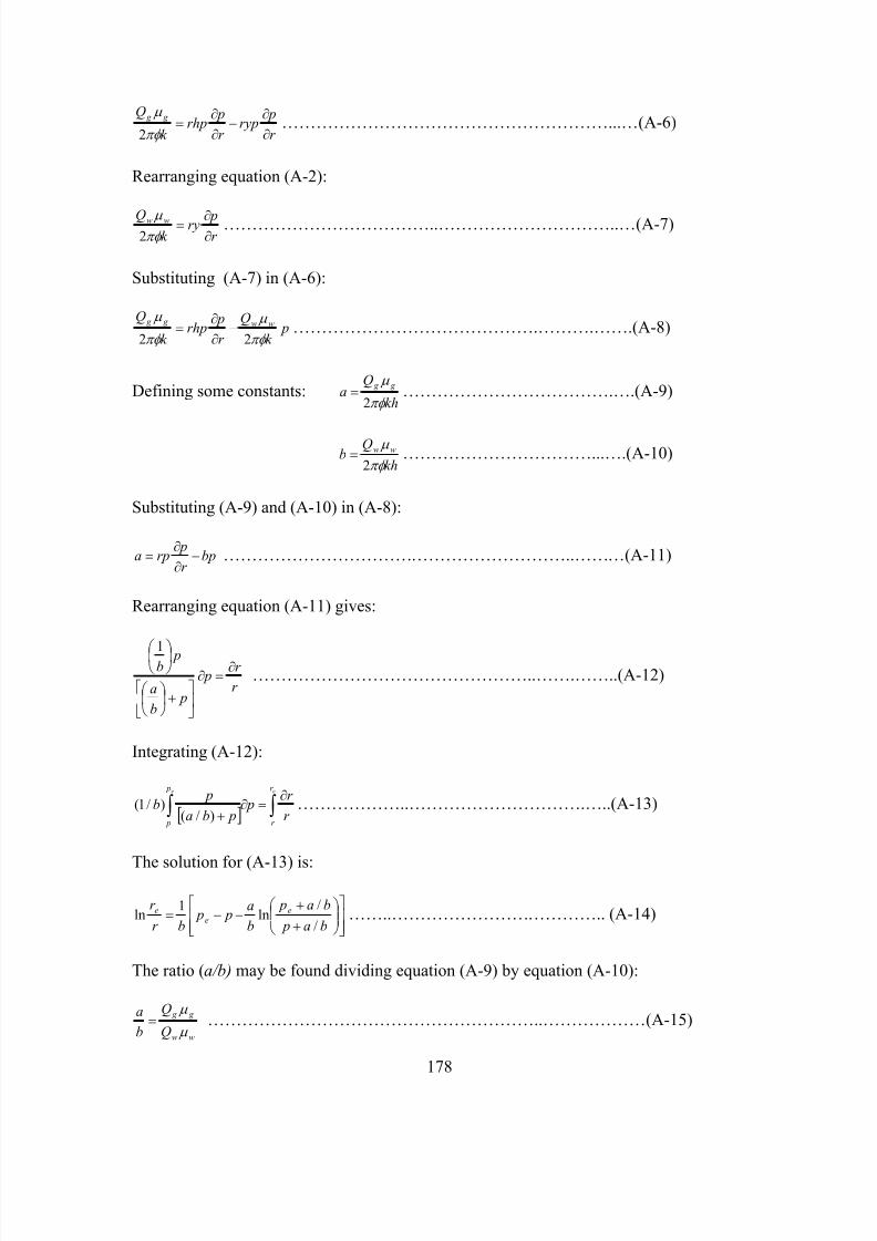
7/23/2019 Armenta Dis
http://slidepdf.com/reader/full/armenta-dis 196/263
r
pryp
r
prhp
k
Q g g
∂
∂−
∂
∂=
πφ
µ
2…………………………………………………...…(A-6)
Rearranging equation (A-2):
r pry
k Q ww
∂∂=
πφ µ
2………………………………..…………………………..…(A-7)
Substituting (A-7) in (A-6):
pk
Q
r
prhp
k
Qww g g
πφ
µ
πφ
µ
22−
∂
∂= …………………………………….……….…….(A-8)
Defining some constants:kh
Qa
g g
πφ
µ
2= ……………………………….….(A-9)
kh
Qb
ww
πφ
µ
2= ……………………………...….(A-10)
Substituting (A-9) and (A-10) in (A-8):
bpr
prpa −
∂
∂= ……………………………………………………..………(A-11)
Rearranging equation (A-11) gives:
r
r p
pb
a
pb ∂
=∂
+
1
…………………………………………..…….……..(A-12)
Integrating (A-12):
[ ] ∫∫ ∂
=∂+
ee r
r
p
p r
r p
pba
pb
)/()/1( ………………..………………………….…..(A-13)
The solution for (A-13) is:
+
+−−=
ba p
ba p
b
a p p
br
r ee
e
/
/ln
1ln ……..……………………………….. (A-14)
The ratio (a/b) may be found dividing equation (A-9) by equation (A-10):
ww
g g
Q
Q
b
a
µ
µ = …………………………………………………..………………(A-15)
178

7/23/2019 Armenta Dis
http://slidepdf.com/reader/full/armenta-dis 197/263
From equation (A-4):
b
a p
h y
h y
Q
Qe
e
e
ww
g g =
−=
)/(
)/(1
µ
µ ………………………………………..…………(A-16)
The ratio (1/b) can be found from equation (A-14) at the wellbore (r = r w ⇒ p = pw):
+
+
−−
=
)/(
)/(ln)(
ln1
ba p
ba p
b
a p p
r
r
b
w
ewe
w
e
…………………………………………(A-17)
Finally, y may be solved from equation (A-3) and (A-15):
b
a
y
p yh
Q
Q
ww
g g =
−=
)(
µ
µ ⇒
[ ] pba
hp y
+
=)/(
……………………………………..(A-18)
Repeating the same analysis for the oil-water system:
r
pk yhr Q
o
o∂
∂−=
µ
φ π )(2…………………………………………….……..…..(A-19)
r
pryk Q
w
w∂
∂=
µ
φ π 2………………………………………………………..…..(A-20)
y
yh
Q
Q
Ro
w
w
o
µ
µ )( −
== ………………………………………………………...(A-21)
If:kh
Qa oo
πφ
µ
2= , and
kh
Q ww
πφ b
µ
2= , then
e
e
ww
oo
y
yh
Q
Q
b
a )( −==
µ
µ ………….……..(A-22)
Rearranging Eq. A-19:r
pry
r
prh
k
Q oo
∂
∂−
∂
∂=
πφ
µ
2………………………...…..(A-23)
Integrating (A-23):
∫∫ ∂=∂
+
ee p
p
r
r p
br r
ba 11 …………………………………………………….(A-24)
( )
+
−
=
1
1
ln
b
a
p pb
r
r e
e ……………………………………………….……..(A-25)
179

7/23/2019 Armenta Dis
http://slidepdf.com/reader/full/armenta-dis 198/263
Solving for y:
+
=
1b
a
h y ……………………………………….……..(A-26)
180

7/23/2019 Armenta Dis
http://slidepdf.com/reader/full/armenta-dis 199/263
APPENDIX B
EXAMPLE ECLIPSE DATA DECK FOR COMPARISON OF WATER CONING
IN OIL AND GAS WELLS AFTER WATER BREAKTHROUGH
GAS-WATER MODEL
RunspecTitleComparison of Water Coning in Oil and Gas Wells After WaterBreakthroughGas-Water Model
MESSAGES
6* 3*5000 /RadialDimens-- NR Theta NZ
26 1 128 /
GasWaterFieldRegdims2 /
Welldims-- Wells Con Group Well in group
2 100 1 2 /
VFPPDIMS10 10 10 10 0 2 /
Start1 'Jan' 2002 /
Nstack300 /
Unifout-------------------------------------------------------------GridTops26*5000 /
Inrad0.333 /
DRV0.4170 0.3016 0.4229 0.5929 0.8313 1.1661.634 2.292 3.213 4.505 6.317 8.85712.42 17.41 24.41 34.23 48.00 67.3094.36 132.3 185.5 260.1 364.7 511.4717.0 2500 /
DZ
3120*0.5182*526*550
/Equals'DTHETA' 360 /'PERMR' 10 /
'PERMTHT' 100 /'PERMZ' 5 /'PORO' 0.25 /'PORO' 0 26 26 1 1 1 100 /'PORO' 10 26 26 1 1 101 128 /
181

7/23/2019 Armenta Dis
http://slidepdf.com/reader/full/armenta-dis 200/263
/INIT--RPTGRID--1 /-------------------------------------------------------------
PROPSDENSITY
45 64 0.046 /ROCK
2500 10E-6 /PVTW
2500 1 2.6E-6 0.68 0 /
PVZG-- Temperature120 /
-- Press Z Visc100 0.989 0.0122300 0.967 0.0124
500 0.947 0.0126700 0.927 0.0129900 0.908 0.0133
1100 0.891 0.01371300 0.876 0.01411500 0.863 0.01461700 0.853 0.0151
1900 0.845 0.01572100 0.840 0.01632300 0.837 0.01672500 0.837 0.01772700 0.839 0.01843200 0.844 0.0202
/
--Saturation Functions--Sgc = 0.20--Krg @ Swir = 0.9--Swir = 0.3--Sorg = 0.0SGFN--Using Honarpour Equation 71
-- Sg Krg Pc0.00 0.000 0.00.10 0.000 0.00.20 0.020 0.00.30 0.030 0.00.40 0.081 0.0
0.50 0.183 0.00.60 0.325 0.00.70 0.900 0.0
/SWFN
--Using Honarpour Equation 67-- Sw Krw Pc
0.3 0.000 0.00.4 0.035 0.00.5 0.076 0.00.6 0.126 0.00.7 0.193 0.00.8 0.288 0.00.9 0.422 0.0
1.0 1.000 0.0/
182

7/23/2019 Armenta Dis
http://slidepdf.com/reader/full/armenta-dis 201/263
-------------------------------------------------------------REGIONSFipnum2600*1728*2
/-------------------------------------------------------------
SOLUTIONEQUIL
5000 1500 5050 0 5050 0 /RPTSOL6* 2 2 /
-------------------------------------------------------------SUMMARYSEPARATERPTONLYWGPR/
WWPR/WBHP
/WTHP/WGPT
/WWPT/WBP/RGIP/
RPR1 2 /TCPU-------------------------------------------------------------SCHEDULENOECHOINCLUDE
'WELL-5000-VI.VFP' /ECHORPTSCHED
6* 2 /RPTRST
4 / restarts once a year
TUNING0.0007 30.4 0.0007 0.0007 1.2 /3* 0.00001 3* 0.0001 /2* 500 1* 100 /
WELSPECS
'P' 'G' 1 1 5000 'GAS' 2* 'STOP' 'YES' //
COMPDAT'P' 1 1 1 100 'OPEN' 2* 0.666 /
/WCONPROD'P' 'OPEN' 'THP' 6* 300 1 /
/WECON
'P' 1* 1000 3* 'WELL' 'YES' //
183

7/23/2019 Armenta Dis
http://slidepdf.com/reader/full/armenta-dis 202/263
TSTEP6*30.4 /
TSTEP48*30.4 /
TSTEP
35*30.4 /TSTEP
48*30.4 /TSTEP48*30.4 /
TSTEP48*30.4 /
TSTEP48*30.4 /
TSTEP48*30.4 /
TSTEP48*30.4 /
TSTEP48*30.4 /
TSTEP
48*30.4 /TSTEP48*30.4 /
TSTEP
48*30.4 /TSTEP48*30.4 /
TSTEP48*30.4 /
TSTEP48*30.4 /
TSTEP48*30.4 /
TSTEP48*30.4 /
TSTEP48*30.4 /
TSTEP
48*30.4 /TSTEP48*30.4 /
TSTEP48*30.4 /
TSTEP
48*30.4 /TSTEP48*30.4 /
TSTEP48*30.4 /
TSTEP48*30.4 /
TSTEP48*30.4 /
TSTEP48*30.4 /
TSTEP48*30.4 /
End
184

7/23/2019 Armenta Dis
http://slidepdf.com/reader/full/armenta-dis 203/263
ECLIPSE VFP INCLUDED FILE: WELL-5000-VI
VFPPROD
1 5.00000E+003 'GAS' 'WGR' 'OGR' 'THP' '' 'FIELD' 'BHP'/
5.00000E+002 1.00000E+003 3.00000E+003 5.00000E+0031.00000E+004 1.50000E+004 1.80000E+004 /
3.00000E+002 5.00000E+002 7.00000E+002 /0.00000E+000 5.00000E-002 1.00000E-001 2.00000E-0014.00000E-001 6.00000E-001 8.00000E-001 1.00000E+000 /
0.00000E+000 /0.00000E+000 /
1 1 1 1 3.37024E+002 3.45916E+002 4.25316E+002 5.47796E+0029.16800E+002 1.30649E+003 1.53942E+003 /
2 1 1 1 5.59849E+002 5.65127E+002 6.15848E+002 7.04360E+002
1.01422E+003 1.37324E+003 1.59511E+003 /3 1 1 1 7.84870E+002 7.88564E+002 8.24884E+002 8.91574E+002
1.14823E+003 1.47144E+003 1.67903E+003 /1 2 1 1 1.00767E+003 6.85715E+002 5.26979E+002 6.66317E+002
1.17821E+003 1.69683E+003 2.00157E+003 /
2 2 1 1 1.33083E+003 1.14235E+003 7.95789E+002 8.23119E+0021.26153E+003 1.75038E+003 2.04461E+003 /
3 2 1 1 1.63681E+003 1.43549E+003 1.08259E+003 1.05816E+0031.38041E+003 1.83132E+003 2.11135E+003 /
1 3 1 1 1.02840E+003 7.98358E+002 6.46858E+002 7.92196E+0021.40325E+003 2.01561E+003 2.37484E+003 /
2 3 1 1 1.35532E+003 1.17999E+003 9.33680E+002 9.70272E+0021.48036E+003 2.06380E+003 2.41335E+003 /
3 3 1 1 1.66413E+003 1.46993E+003 1.24089E+003 1.22716E+003
1.59380E+003 2.13846E+003 2.47443E+003 /1 4 1 1 1.06877E+003 9.06174E+002 8.40372E+002 1.03062E+003
1.79136E+003 2.60038E+003 3.08950E+003 /2 4 1 1 1.40292E+003 1.23965E+003 1.14544E+003 1.22814E+003
1.87547E+003 2.65034E+003 3.12890E+003 /
3 4 1 1 1.71647E+003 1.53687E+003 1.43807E+003 1.50399E+0032.00566E+003 2.72983E+003 3.19348E+003 /
1 5 1 1 1.14745E+003 1.03248E+003 1.14282E+003 1.50309E+0032.63140E+003 3.81908E+003 4.60402E+003 /
2 5 1 1 1.49259E+003 1.35495E+003 1.42442E+003 1.68890E+0032.70978E+003 3.86469E+003 4.64024E+003 /
3 5 1 1 1.81241E+003 1.66240E+003 1.68147E+003 1.92590E+0032.82769E+003 3.93860E+003 4.70113E+003 /
1 6 1 1 1.22282E+003 1.13624E+003 1.39809E+003 1.90174E+0033.33657E+003 4.76408E+003 5.69293E+003 /
2 6 1 1 1.57486E+003 1.46356E+003 1.65458E+003 2.07013E+0033.40719E+003 4.80311E+003 5.72329E+003 /
3 6 1 1 1.89758E+003 1.77592E+003 1.89757E+003 2.26855E+0033.51185E+003 4.86696E+003 5.77621E+003 /
1 7 1 1 1.29426E+003 1.23434E+003 1.62877E+003 2.24629E+0033.93384E+003 5.78065E+003 7.03960E+003 /2 7 1 1 1.65009E+003 1.56415E+003 1.86048E+003 2.39607E+003
4.00224E+003 5.81806E+003 7.06883E+003 /3 7 1 1 1.97324E+003 1.87771E+003 2.09286E+003 2.57229E+003
4.09229E+003 5.87715E+003 7.11864E+003 /1 8 1 1 1.36153E+003 1.32752E+003 1.83827E+003 2.56051E+003
4.54574E+003 6.91460E+003 8.57619E+003 /
2 8 1 1 1.71853E+003 1.65684E+003 2.04934E+003 2.69480E+0034.60380E+003 6.95034E+003 8.60433E+003 /
3 8 1 1 2.04060E+003 1.96914E+003 2.27214E+003 2.85658E+0034.68526E+003 7.00651E+003 8.65222E+003 /
185

7/23/2019 Armenta Dis
http://slidepdf.com/reader/full/armenta-dis 204/263
EXAMPLE ECLIPSE DATA DECK FOR COMPARISON OF WATER CONING
IN OIL AND GAS WELLS AFTER WATER BREAKTHROUGH
OIL-WATER MODEL
RunspecTitleComparison of Water Coning in Oil and Gas Well After Water
BreakthroughOil-Water Model
MESSAGES6* 3*5000 /Radial
Dimens-- NR Theta NZ
26 1 128 /NONNCOil
--Gas--Disgas
WaterFieldRegdims2 /
Welldims-- Wells Con Group Well in group
2 100 1 2 /
VFPPDIMS10 10 10 10 0 2 /
Start1 'Jan' 2002 /
Nstack
300 /Unifout-------------------------------------------------------------GridTops26*5000 /
Inrad0.333 /
DRV0.4170 0.3016 0.4229 0.5929 0.8313 1.1661.634 2.292 3.213 4.505 6.317 8.85712.42 17.41 24.41 34.23 48.00 67.3094.36 132.3 185.5 260.1 364.7 511.4717.0 2500 /
DZ3120*0.5182*526*550
/Equals'DTHETA' 360 /
'PERMR' 10 /'PERMTHT' 100 /'PERMZ' 5 /'PORO' 0.25 /'PORO' 0 26 26 1 1 1 100 /
186

7/23/2019 Armenta Dis
http://slidepdf.com/reader/full/armenta-dis 205/263
'PORO' 10 26 26 1 1 101 128 //INIT--RPTGRID--1 /
-------------------------------------------------------------PROPS
DENSITY45 64 0.046 /
ROCK2500 10E-6 /
PVTW
2500 1 2.6E-6 0.68 0 /
SWOF-- Sw Krw Krow Pcow
0.27 0.000 0.900 00.35 0.012 0.596 0
0.40 0.032 0.438 00.45 0.061 0.304 00.50 0.099 0.195 0
0.55 0.147 0.110 00.60 0.204 0.049 00.65 0.271 0.012 00.70 0.347 0.000 0 /
PVCDO2500 1.15 1.5E-5 0.5 0 /
RSCONST0.379 1000
/-------------------------------------------------------------
REGIONSFipnum2600*1728*2
/-------------------------------------------------------------SOLUTION
EQUIL5000 3000 5050 0 100 0 1 1 2* /
RPTSOL6* 2 2 /
-------------------------------------------------------------SUMMARY
SEPARATERPTONLYWOPR/WWPR
/WBHP
/WTHP/WOPT/WWPT/
WBP/
187

7/23/2019 Armenta Dis
http://slidepdf.com/reader/full/armenta-dis 206/263
RGIP/RPR1 2 /TCPU
-------------------------------------------------------------SCHEDULE
NOECHO--INCLUDE--'WELL-5000-VI.VFP' /ECHORPTSCHED
6* 2 /RPTRST
4 / restarts once a yearTUNING0.0007 30.4 0.0007 0.0007 1.2 /3* 0.00001 3* 0.0001 /
2* 500 1* 100 /WELSPECS'P' 'G' 1 1 5000 'GAS' 2* 'STOP' 'YES' /
/COMPDAT'P' 1 1 1 100 'OPEN' 2* 0.666 /
/
WCONPROD'P' 'OPEN' 'ORAT' 630 /
/WECON'P' 2* 1.0 2* 'WELL' 'YES' /
/TSTEP
6*30.4 /TSTEP48*30.4 /
TSTEP35*30.4 /
TSTEP48*30.4 /
TSTEP48*30.4 /
TSTEP48*30.4 /
TSTEP48*30.4 /
TSTEP48*30.4 /
TSTEP48*30.4 /
TSTEP
48*30.4 /TSTEP
48*30.4 /TSTEP48*30.4 /
TSTEP48*30.4 /
TSTEP48*30.4 /
TSTEP48*30.4 /
188

7/23/2019 Armenta Dis
http://slidepdf.com/reader/full/armenta-dis 207/263
189
TSTEP48*30.4 /
TSTEP48*30.4 /
TSTEP
48*30.4 /TSTEP
48*30.4 /TSTEP48*30.4 /
TSTEP48*30.4 /
TSTEP48*30.4 /
TSTEP48*30.4 /
TSTEP48*30.4 /
TSTEP48*30.4 /
TSTEP
48*30.4 /TSTEP48*30.4 /
TSTEP
48*30.4 /TSTEP48*30.4 /
TSTEP48*30.4 /
TSTEP48*30.4 /
TSTEP48*30.4 /
TSTEP48*30.4 /
TSTEP48*30.4 /
TSTEP
48*30.4 /TSTEP48*30.4 /
TSTEP48*30.4 /
TSTEP
48*30.4 /TSTEP48*30.4 /
TSTEP48*30.4 /
TSTEP48*30.4 /
End

7/23/2019 Armenta Dis
http://slidepdf.com/reader/full/armenta-dis 208/263
APPENDIX C
EXAMPLE ECLIPSE DATA DECK FOR EFFECT OF VERTICAL
PERMEABILITY ON WATER CONING
Runspec
TitleEffect of Vertical Permeability on Water ConingVertical Permeability equal to 30% Horizontal Permeability
MESSAGES6* 3*5000 /RadialDimens-- NR Theta NZ
26 1 110 /GasWaterField
Regdims2 /Welldims-- Wells Con
1 100 /VFPPDIMS10 10 10 10 0 1 /
Start1 'Jan' 1998 /
Nstack100 /
Unifout-------------------------------------------------------------Grid
Tops26*5000 /
Inrad0.333 /
DRV0.4170 0.3016 0.4229 0.5929 0.8313 1.1661.634 2.292 3.213 4.505 6.317 8.85712.42 17.41 24.41 34.23 48.00 67.3094.36 132.3 185.5 260.1 364.7 511.4717.0 2500 /
DZ2600*1234*10
26*110/Equals'DTHETA' 360 /'PERMR' 10 /'PERMTHT' 10 /'PERMZ' 3 /'PORO' 0.25 /'PORO' 0 26 26 1 1 1 100 /'PORO' 10 26 26 1 1 101 110 /
/
190

7/23/2019 Armenta Dis
http://slidepdf.com/reader/full/armenta-dis 209/263
INIT--RPTGRID--1 /-------------------------------------------------------------PROPSDENSITY45 64 0.046 /
ROCK2500 10E-6 /
PVTW2500 1 2.6E-6 0.68 0 /
PVZG-- Temperature120 /
-- Press Z Visc100 0.989 0.0122300 0.967 0.0124500 0.947 0.0126700 0.927 0.0129900 0.908 0.0133
1100 0.891 0.01371300 0.876 0.01411500 0.863 0.01461700 0.853 0.01511900 0.845 0.01572100 0.840 0.01632300 0.837 0.01672500 0.837 0.01772700 0.839 0.0184
/--Saturation Functions--Sgc = 0.20--Krg @ Swir = 0.9--Swir = 0.3--Sorg = 0.0SGFN--Using Honarpour Equation 71-- Sg Krg Pc
0.00 0.000 0.00.20 0.000 0.00.30 0.020 0.00.40 0.081 0.00.50 0.183 0.00.60 0.325 0.00.70 0.900 0.0
/SWFN
--Using Honarpour Equation 67-- Sw Krw Pc0.3 0.000 0.00.4 0.035 0.00.5 0.076 0.00.6 0.126 0.00.7 0.193 0.00.8 0.288 0.00.9 0.422 0.01.0 1.000 0.0
/
191

7/23/2019 Armenta Dis
http://slidepdf.com/reader/full/armenta-dis 210/263
-------------------------------------------------------------REGIONSFipnum2600*1260*2
/-------------------------------------------------------------SOLUTIONEQUIL
5000 2300 5100 0 5100 0 /RPTSOL6* 2 2 /
-------------------------------------------------------------SUMMARYSEPARATERPTONLYWGPR/WWPR/
WBHP/WTHP/WGPT/WWPT/WBP/RGIP/RPR1 2 /TCPU-------------------------------------------------------------SCHEDULENOECHOINCLUDE'WELL-5000-VI.VFP' /
ECHORPTSCHED
6* 2 /RPTRST
4 / restarts once a yearTUNING0.0007 30.4 0.0007 0.0007 1.2 /
3* 0.00001 3* 0.0001 /2* 100 /
WELSPECS'P' 'G' 1 1 5000 'GAS' 2* 'STOP' 'YES' /
/COMPDAT'P' 1 1 1 30 'OPEN' 2* 0.666 /
/WCONPROD'P' 'OPEN' 'THP' 5* 550 500 1 /
/
192

7/23/2019 Armenta Dis
http://slidepdf.com/reader/full/armenta-dis 211/263
WECON'P' 1* 1220 4* 'YES' /
/TSTEP48*30.4 /
TSTEP48*30.4 /
TSTEP48*30.4 /
TSTEP48*30.4 /
TSTEP48*30.4 /
TSTEP48*30.4 /
TSTEP48*30.4 /
TSTEP48*30.4 /
TSTEP
48*30.4 /TSTEP48*30.4 /
TSTEP48*30.4 /
TSTEP48*30.4 /
End
193

7/23/2019 Armenta Dis
http://slidepdf.com/reader/full/armenta-dis 212/263
EXAMPLE ECLIPSE DATA DECK FOR EFFECT OF AQUIFER SIZE ON
WATER CONING
RunspecTitleEffect of Aquifer Size on Water Coning
VAD equal to 519
MESSAGES6* 3*5000 /RadialDimens-- NR Theta NZ
26 1 110 /GasWaterFieldRegdims2 /
Welldims-- Wells Con
1 100 /VFPPDIMS10 10 10 10 0 1 /
Start1 'Jan' 1998 /
Nstack100 /
Unifout-------------------------------------------------------------GridTops26*5000 /
Inrad0.333 /
DRV0.4170 0.3016 0.4229 0.5929 0.8313 1.1661.634 2.292 3.213 4.505 6.317 8.85712.42 17.41 24.41 34.23 48.00 67.3094.36 132.3 185.5 260.1 364.7 511.4717.0 2500 /
DZ2600*1234*1026*410
/Equals'DTHETA' 360 /'PERMR' 10 /'PERMTHT' 10 /'PERMZ' 1 /'PORO' 0.25 /'PORO' 0 26 26 1 1 1 100 /'PORO' 10 26 26 1 1 101 110 /
/INIT--RPTGRID--1 /
194

7/23/2019 Armenta Dis
http://slidepdf.com/reader/full/armenta-dis 213/263
-------------------------------------------------------------PROPSDENSITY45 64 0.046 /
ROCK2500 10E-6 /
PVTW2500 1 2.6E-6 0.68 0 /
PVZG-- Temperature120 /
-- Press Z Visc100 0.989 0.0122300 0.967 0.0124500 0.947 0.0126700 0.927 0.0129900 0.908 0.01331100 0.891 0.01371300 0.876 0.01411500 0.863 0.0146
1700 0.853 0.01511900 0.845 0.01572100 0.840 0.01632300 0.837 0.01672500 0.837 0.01772700 0.839 0.0184
/--Saturation Functions--Sgc = 0.20--Krg @ Swir = 0.9--Swir = 0.3--Sorg = 0.0SGFN--Using Honarpour Equation 71-- Sg Krg Pc
0.00 0.000 0.00.20 0.000 0.00.30 0.020 0.00.40 0.081 0.00.50 0.183 0.00.60 0.325 0.00.70 0.900 0.0
/SWFN--Using Honarpour Equation 67-- Sw Krw Pc0.3 0.000 0.0
0.4 0.035 0.00.5 0.076 0.00.6 0.126 0.00.7 0.193 0.00.8 0.288 0.00.9 0.422 0.01.0 1.000 0.0
/-------------------------------------------------------------REGIONSFipnum
195

7/23/2019 Armenta Dis
http://slidepdf.com/reader/full/armenta-dis 214/263

7/23/2019 Armenta Dis
http://slidepdf.com/reader/full/armenta-dis 215/263
TSTEP48*30.4 /
TSTEP48*30.4 /
TSTEP48*30.4 /
TSTEP48*30.4 /
TSTEP48*30.4 /
TSTEP48*30.4 /
TSTEP48*30.4 /
TSTEP48*30.4 /
TSTEP48*30.4 /
TSTEP48*30.4 /
TSTEP48*30.4 /
TSTEP48*30.4 /
End
197

7/23/2019 Armenta Dis
http://slidepdf.com/reader/full/armenta-dis 216/263
EXAMPLE ECLIPSE DATA DECK FOR EFFECT OF FLOW BEHIND CASING
ON WATER CONING
Runspec
TitleEffect of Flow Behind CasingChannel Size 1.3 inches (Permeability in the first grid 1,000,000 md)Channel Initially in the Water Zone
6* 3*5000 /RadialDimens-- NR Theta NZ
26 1 110 /GasWaterFieldRegdims2 /
Welldims-- Wells Con
1 100 /VFPPDIMS10 10 10 10 0 1 /
Start1 'Jan' 1998 /
Nstack100 /
Unifout-------------------------------------------------------------Grid
Tops26*5000 /
Inrad0.333 /
DRV0.4170 0.3016 0.4229 0.5929 0.8313 1.1661.634 2.292 3.213 4.505 6.317 8.85712.42 17.41 24.41 34.23 48.00 67.3094.36 132.3 185.5 260.1 364.7 511.4717.0 2500 /
DZ2600*1234*1026*110
/Equals'DTHETA' 360 /'PERMR' 100 /'PERMTHT' 100 /'PERMZ' 10 /'PORO' 0.25 /'PORO' 0 26 26 1 1 1 100 /'PORO' 10 26 26 1 1 101 110 /'PERMZ' 1000000 1 1 1 1 1 101 /'PERMR' 0 1 1 1 1 51 100 /
198
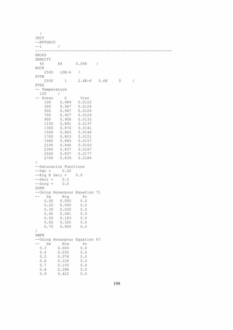
7/23/2019 Armenta Dis
http://slidepdf.com/reader/full/armenta-dis 217/263
/
INIT--RPTGRID--1 /-------------------------------------------------------------PROPSDENSITY45 64 0.046 /
ROCK2500 10E-6 /
PVTW2500 1 2.6E-6 0.68 0 /
PVZG-- Temperature120 /
-- Press Z Visc100 0.989 0.0122300 0.967 0.0124500 0.947 0.0126
700 0.927 0.0129900 0.908 0.01331100 0.891 0.01371300 0.876 0.01411500 0.863 0.01461700 0.853 0.01511900 0.845 0.01572100 0.840 0.01632300 0.837 0.01672500 0.837 0.01772700 0.839 0.0184
/--Saturation Functions--Sgc = 0.20--Krg @ Swir = 0.9--Swir = 0.3--Sorg = 0.0SGFN--Using Honarpour Equation 71-- Sg Krg Pc
0.00 0.000 0.00.20 0.000 0.00.30 0.020 0.00.40 0.081 0.00.50 0.183 0.00.60 0.325 0.00.70 0.900 0.0
/SWFN--Using Honarpour Equation 67-- Sw Krw Pc0.3 0.000 0.00.4 0.035 0.00.5 0.076 0.00.6 0.126 0.00.7 0.193 0.00.8 0.288 0.00.9 0.422 0.0
199

7/23/2019 Armenta Dis
http://slidepdf.com/reader/full/armenta-dis 218/263
1.0 1.000 0.0/-------------------------------------------------------------REGIONSFipnum2600*1260*2
/-------------------------------------------------------------SOLUTIONEQUIL
5000 2500 5100 0 5100 0 /RPTSOL6* 2 2 /
-------------------------------------------------------------SUMMARYSEPARATERPTONLYWGPR/
WWPR/WBHP/WTHP/WGPT/WWPT/WBP/RGIP/RPR1 2 /TCPU-------------------------------------------------------------SCHEDULENOECHOINCLUDE'GWVFP.VFP' /
ECHORPTSCHED
6* 2 /RPTRST
4 / restarts once a year
TUNING0.0007 30.4 0.0007 0.0007 1.2 /3* 0.00001 3* 0.0001 /2* 100 /
WELSPECS'P' 'G' 1 1 5000 'GAS' 2* 'STOP' 'YES' /
/COMPDAT'P' 1 1 1 50 'OPEN' 2* 0.666 /
/WCONPROD
200

7/23/2019 Armenta Dis
http://slidepdf.com/reader/full/armenta-dis 219/263
'P' 'OPEN' 'BHP' 2* 25000 2* 2000 1* 1 //WECON'P' 1* 1220 4* 'YES' /
/TSTEP12*30.4 /
TSTEP12*30.4 /
TSTEP6*30.4 /TSTEP48*30.4 /
TSTEP48*30.4 /
TSTEP48*30.4 /
TSTEP48*30.4 /
TSTEP
48*30.4 /TSTEP48*30.4 /
TSTEP48*30.4 /
TSTEP48*30.4 /
End
201

7/23/2019 Armenta Dis
http://slidepdf.com/reader/full/armenta-dis 220/263
EXAMPLE IMEX DATA DECK FOR EFFECT OF NON-DARCY FLOW ON
WATER CONING
Effect of Non-Darcy Effect on Water ConingNon-Darcy Flow Effect Distributed in the Reservoir
RESULTS SIMULATOR IMEXRESULTS SECTION INOUT**SS-UNKNOWN** REGDIMS** 2 /**SS-ENDUNKNOWN**SS-UNKNOWN** INIT** --RPTGRID** --1 /** -------------------------------------------------------------**SS-ENDUNKNOWN*DIM *MAX_WELLS 1
*DIM *MAX_LAYERS 100
******************************************************************************** *IO*******************************************************************************TITLE1
**Effect of Non-Darcy Effect on Water Coning**Non-Darcy Flow Effect Distributed in the Reservoir**------------------------------------------------------------
**SS-NOEFFECT** MESSAGES** 6* 3*5000 /**SS-ENDNOEFFECT**------------------------------------------------------------*INUNIT *FIELD
*OUTUNIT *FIELD
GRID RADIAL 26 1 110 RW 3.33000000E-1KDIR DOWN
DI IVAR
0.417 0.3016 0.4229 0.5929 0.8313 1.166 1.634 2.292 3.213 4.5056.317 8.85712.42 17.41 24.41 34.23 48. 67.3 94.36 132.3 185.5 260.1 364.7
511.4 717.2500.
DJ CON 360.
DK KVAR100*1. 9*10. 210.
202

7/23/2019 Armenta Dis
http://slidepdf.com/reader/full/armenta-dis 221/263
DTOP26*5000.
RESULTS SECTION GRIDRESULTS SECTION NETPAYRESULTS SECTION NETGROSSRESULTS SECTION POR
**$ RESULTS PROP POR Units: Dimensionless**$ RESULTS PROP Minimum Value: 0 Maximum Value: 1POR ALL
2860*1.MOD 1:26 1:1 1:110 = 0.1
26:26 1:1 1:100 = 026:26 1:1 101:110 = 1
RESULTS SECTION PERMS
**$ RESULTS PROP PERMI Units: md
**$ RESULTS PROP Minimum Value: 10 Maximum Value: 10PERMI ALL
2860*1.MOD 1:26 1:1 1:110 = 10
**$ RESULTS PROP PERMJ Units: md**$ RESULTS PROP Minimum Value: 10 Maximum Value: 10PERMJ ALL
2860*1.MOD 1:26 1:1 1:110 = 10
**$ RESULTS PROP PERMK Units: md**$ RESULTS PROP Minimum Value: 1 Maximum Value: 1PERMK ALL
2860*1.MOD 1:26 1:1 1:110 = 1RESULTS SECTION TRANSRESULTS SECTION FRACSRESULTS SECTION GRIDNONARRAYSCPOR MATRIX 1.E-05PRPOR MATRIX 2500.
RESULTS SECTION VOLMODRESULTS SECTION SECTORLEASE**$ SECTORARRAY 'SECTOR1' Definition.SECTORARRAY 'SECTOR1' ALL
2600*1 260*0
**$ SECTORARRAY 'SECTOR2' Definition.SECTORARRAY 'SECTOR2' ALL
2600*0 260*1
RESULTS SECTION ROCKCOMPACTIONRESULTS SECTION GRIDOTHERRESULTS SECTION MODELMODEL *BLACKOIL**$ OilGas Table 'Table A'
203

7/23/2019 Armenta Dis
http://slidepdf.com/reader/full/armenta-dis 222/263
*TRES 120.*PVT *EG 1** P Rs Bo EG VisO VisG
14.7 5.51 1.0268 5.05973 1.2801 0.011983213.72 47.23 1.0414 75.1695 1.0556 0.01216412.74 97.95 1.0599 148.3052 0.8894 0.0124611.76 153.78 1.0811 224.457 0.7705 0.01268810.78 213.36 1.1045 303.5186 0.6824 0.0129931009.8 275.94 1.1299 385.257 0.6146 0.0133351208.82 341.06 1.1571 469.289 0.5609 0.0137051407.84 408.36 1.1859 555.068 0.5173 0.0141031606.86 477.62 1.2163 641.895 0.481 0.0145281805.88 548.62 1.2481 728.959 0.4504 0.014982004.9 621.23 1.2813 815.4 0.4241 0.015462203.92 695.32 1.3158 900.389 0.4013 0.0159692402.94 770.77 1.3515 983.192 0.3813 0.0165082601.96 847.5 1.3885 1063.222 0.3636 0.0170772800.98 925.44 1.4265 1140.054 0.3479 0.0176783000. 1004.5 1.4657 1213.424 0.3337 0.018313
*DENSITY *OIL 50.0004
*DENSITY *GAS 0.046*DENSITY *WATER 63.9098*CO 1.777275E-05*BWI 1.003357*CW 2.934065E-06*REFPW 2500.*VWI 0.658209*CVW 0
RESULTS SECTION MODELARRAYSRESULTS SECTION ROCKFLUID******************************************************************************** *ROCKFLUID******************************************************************************
*ROCKFLUID
*RPT 1*SWT0.300000 0.000000 1.000000 0.0000000.400000 0.035000 0.857142857142857 0.0000000.500000 0.076000 0.714285714285714 0.000000
0.600000 0.126000 0.571428571428572 0.0000000.700000 0.193000 0.428571428571429 0.0000000.800000 0.288000 0.285714285714286 0.0000000.900000 0.422000 0.142857142857143 0.0000001.000000 1.000000 0.000000 0.000000
*SGT *NOSWC0.000000 0.000000 1.000000 0.0000000.200000 0.000000 0.714285714285714 0.0000000.300000 0.020000 0.571428571428572 0.0000000.400000 0.081000 0.428571428571429 0.000000
204
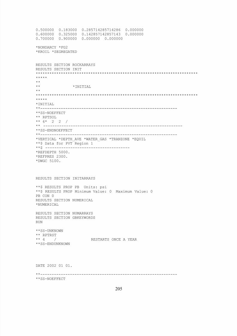
7/23/2019 Armenta Dis
http://slidepdf.com/reader/full/armenta-dis 223/263
0.500000 0.183000 0.285714285714286 0.0000000.600000 0.325000 0.142857142857143 0.0000000.700000 0.900000 0.000000 0.000000
*NONDARCY *FG2*KROIL *SEGREGATED
RESULTS SECTION ROCKARRAYSRESULTS SECTION INIT******************************************************************************** *INITIAL*******************************************************************************INITIAL**------------------------------------------------------------**SS-NOEFFECT
** RPTSOL** 6* 2 2 /** -------------------------------------------------------------**SS-ENDNOEFFECT**------------------------------------------------------------*VERTICAL *DEPTH_AVE *WATER_GAS *TRANZONE *EQUIL**$ Data for PVT Region 1**$ -------------------------------------*REFDEPTH 5000.*REFPRES 2300.*DWGC 5100.
RESULTS SECTION INITARRAYS
**$ RESULTS PROP PB Units: psi**$ RESULTS PROP Minimum Value: 0 Maximum Value: 0PB CON 0RESULTS SECTION NUMERICAL*NUMERICAL
RESULTS SECTION NUMARRAYSRESULTS SECTION GBKEYWORDSRUN
**SS-UNKNOWN
** RPTRST** 4 / RESTARTS ONCE A YEAR**SS-ENDUNKNOWN
DATE 2002 01 01.
**------------------------------------------------------------**SS-NOEFFECT
205

7/23/2019 Armenta Dis
http://slidepdf.com/reader/full/armenta-dis 224/263
** NOECHO**SS-ENDNOEFFECT**------------------------------------------------------------PTUBE WATER_GAS 1DEPTH 5000.QG5.E+05 1.E+06 3.E+06 5.E+06 1.E+07 1.5E+07 1.8E+07WGR0 5.E-05 1.E-04 0.0002 0.0004 0.0006 0.0008 0.001WHP300. 500. 700.BHPTG
1 1 3.37024000E+02 5.59849000E+02 7.84870000E+022 1 1.00767000E+03 1.33083000E+03 1.63681000E+033 1 1.02840000E+03 1.35532000E+03 1.66413000E+034 1 1.06877000E+03 1.40292000E+03 1.71647000E+035 1 1.14745000E+03 1.49259000E+03 1.81241000E+036 1 1.22282000E+03 1.57486000E+03 1.89758000E+037 1 1.29426000E+03 1.65009000E+03 1.97324000E+038 1 1.36153000E+03 1.71853000E+03 2.04060000E+03
1 2 3.45916000E+02 5.65127000E+02 7.88564000E+022 2 6.85715000E+02 1.14235000E+03 1.43549000E+033 2 7.98357000E+02 1.17999000E+03 1.46993000E+034 2 9.06174000E+02 1.23965000E+03 1.53687000E+035 2 1.03248000E+03 1.35495000E+03 1.66240000E+036 2 1.13624000E+03 1.46356000E+03 1.77592000E+037 2 1.23434000E+03 1.56415000E+03 1.87771000E+038 2 1.32752000E+03 1.65684000E+03 1.96914000E+031 3 4.25316000E+02 6.15848000E+02 8.24883000E+022 3 5.26979000E+02 7.95789000E+02 1.08259000E+033 3 6.46858000E+02 9.33680000E+02 1.24089000E+034 3 8.40372000E+02 1.14544000E+03 1.43807000E+035 3 1.14282000E+03 1.42442000E+03 1.68147000E+036 3 1.39809000E+03 1.65458000E+03 1.89757000E+037 3 1.62877000E+03 1.86048000E+03 2.09286000E+038 3 1.83827000E+03 2.04934000E+03 2.27214000E+031 4 5.47796000E+02 7.04360000E+02 8.91575000E+022 4 6.66316000E+02 8.23118000E+02 1.05816000E+033 4 7.92196000E+02 9.70272000E+02 1.22716000E+034 4 1.03062000E+03 1.22814000E+03 1.50399000E+035 4 1.50309000E+03 1.68890000E+03 1.92590000E+036 4 1.90174000E+03 2.07013000E+03 2.26855000E+037 4 2.24629000E+03 2.39607000E+03 2.57229000E+038 4 2.56051000E+03 2.69480000E+03 2.85658000E+031 5 9.16800000E+02 1.01422000E+03 1.14823000E+032 5 1.17821000E+03 1.26153000E+03 1.38041000E+033 5 1.40325000E+03 1.48036000E+03 1.59380000E+03
4 5 1.79136000E+03 1.87547000E+03 2.00566000E+035 5 2.63140000E+03 2.70978000E+03 2.82769000E+036 5 3.33657000E+03 3.40719000E+03 3.51185000E+037 5 3.93384000E+03 4.00224000E+03 4.09229000E+038 5 4.54574000E+03 4.60380000E+03 4.68526000E+031 6 1.30649000E+03 1.37324000E+03 1.47144000E+032 6 1.69683000E+03 1.75038000E+03 1.83132000E+033 6 2.01561000E+03 2.06380000E+03 2.13846000E+034 6 2.60038000E+03 2.65034000E+03 2.72983000E+035 6 3.81908000E+03 3.86469000E+03 3.93860000E+036 6 4.76408000E+03 4.80311000E+03 4.86696000E+03
206

7/23/2019 Armenta Dis
http://slidepdf.com/reader/full/armenta-dis 225/263
7 6 5.78065000E+03 5.81806000E+03 5.87715000E+038 6 6.91460000E+03 6.95034000E+03 7.00651000E+031 7 1.53942000E+03 1.59511000E+03 1.67903000E+032 7 2.00157000E+03 2.04461000E+03 2.11135000E+033 7 2.37484000E+03 2.41335000E+03 2.47443000E+034 7 3.08950000E+03 3.12890000E+03 3.19348000E+035 7 4.60402000E+03 4.64024000E+03 4.70113000E+036 7 5.69293000E+03 5.72329000E+03 5.77622000E+037 7 7.03960000E+03 7.06884000E+03 7.11864000E+038 7 8.57618000E+03 8.60434000E+03 8.65223000E+03
GROUP 'G' ATTACHTO 'FIELD'
WELL 1 'P' ATTACHTO 'G'PRODUCER 'P'PWELLBORE TABLE 5000. 1OPERATE MAX STG 1.E+07 CONTOPERATE MIN BHP 14.7 CONTMONITOR MIN STG 1.2E+06 STOP
GEOMETRY K 0.333 0.37 1. 5.PERF GEO 'P'
1 1 1 1. OPEN1 1 2 1. OPEN1 1 3 1. OPEN1 1 4 1. OPEN1 1 5 1. OPEN1 1 6 1. OPEN1 1 7 1. OPEN1 1 8 1. OPEN1 1 9 1. OPEN1 1 10 1. OPEN1 1 11 1. OPEN1 1 12 1. OPEN1 1 13 1. OPEN1 1 14 1. OPEN1 1 15 1. OPEN1 1 16 1. OPEN1 1 17 1. OPEN1 1 18 1. OPEN1 1 19 1. OPEN1 1 20 1. OPEN1 1 21 1. OPEN1 1 22 1. OPEN1 1 23 1. OPEN1 1 24 1. OPEN
1 1 25 1. OPEN1 1 26 1. OPEN1 1 27 1. OPEN1 1 28 1. OPEN1 1 29 1. OPEN1 1 30 1. OPEN1 1 31 1. OPEN1 1 32 1. OPEN1 1 33 1. OPEN1 1 34 1. OPEN1 1 35 1. OPEN
207

7/23/2019 Armenta Dis
http://slidepdf.com/reader/full/armenta-dis 226/263
1 1 36 1. OPEN1 1 37 1. OPEN1 1 38 1. OPEN1 1 39 1. OPEN1 1 40 1. OPEN1 1 41 1. OPEN1 1 42 1. OPEN1 1 43 1. OPEN1 1 44 1. OPEN1 1 45 1. OPEN1 1 46 1. OPEN1 1 47 1. OPEN1 1 48 1. OPEN1 1 49 1. OPEN1 1 50 1. OPEN1 1 51 1. OPEN1 1 52 1. OPEN1 1 53 1. OPEN1 1 54 1. OPEN1 1 55 1. OPEN
1 1 56 1. OPEN1 1 57 1. OPEN1 1 58 1. OPEN1 1 59 1. OPEN1 1 60 1. OPEN1 1 61 1. OPEN1 1 62 1. OPEN1 1 63 1. OPEN1 1 64 1. OPEN1 1 65 1. OPEN1 1 66 1. OPEN1 1 67 1. OPEN1 1 68 1. OPEN1 1 69 1. OPEN1 1 70 1. OPEN1 1 71 1. OPEN1 1 72 1. OPEN1 1 73 1. OPEN1 1 74 1. OPEN1 1 75 1. OPEN1 1 76 1. OPEN1 1 77 1. OPEN1 1 78 1. OPEN1 1 79 1. OPEN1 1 80 1. OPEN1 1 81 1. OPEN1 1 82 1. OPEN
1 1 83 1. OPEN1 1 84 1. OPEN1 1 85 1. OPEN1 1 86 1. OPEN1 1 87 1. OPEN1 1 88 1. OPEN1 1 89 1. OPEN1 1 90 1. OPEN1 1 91 1. OPEN1 1 92 1. OPEN1 1 93 1. OPEN
208

7/23/2019 Armenta Dis
http://slidepdf.com/reader/full/armenta-dis 227/263
1 1 94 1. OPEN1 1 95 1. OPEN1 1 96 1. OPEN1 1 97 1. OPEN1 1 98 1. OPEN1 1 99 1. OPEN1 1 100 1. OPEN
XFLOW-MODEL 'P' FULLY-MIXED
OPEN 'P'
TIME 30.4
TIME 60.8
TIME 91.2
TIME 121.6
TIME 152
TIME 182.4
TIME 212.8
TIME 243.2
TIME 273.6
TIME 304
TIME 334.4
TIME 364.8
TIME 395.2
TIME 425.6
TIME 456
TIME 486.4
TIME 516.8
TIME 547.2
TIME 577.6
TIME 608
TIME 638.4
TIME 668.8
TIME 699.2
209
7/23/2019 Armenta Dis
http://slidepdf.com/reader/full/armenta-dis 228/263
TIME 729.6
TIME 760
TIME 790.4
TIME 820.8
TIME 851.2
TIME 881.6
TIME 912
TIME 942.4
TIME 972.8
TIME 1003.2
TIME 1033.6
TIME 1064
TIME 1094.4
TIME 1124.8
TIME 1155.2
TIME 1185.6
TIME 1216
TIME 1246.4
TIME 1276.8
TIME 1307.2
TIME 1337.6
TIME 1368
TIME 1398.4
TIME 1428.8
TIME 1459.2
TIME 1489.6
TIME 1520
TIME 1550.4
TIME 1580.8
210

7/23/2019 Armenta Dis
http://slidepdf.com/reader/full/armenta-dis 229/263
TIME 1611.2
TIME 1641.6
TIME 1672
TIME 1702.4
TIME 1732.8
TIME 1763.2
TIME 1793.6
TIME 1824
TIME 1854.4
TIME 1884.8
TIME 1915.2
TIME 1945.6
TIME 1976
TIME 2006.4
TIME 2036.8
TIME 2067.2
TIME 2097.6
TIME 2128
TIME 2158.4
TIME 2188.8
TIME 2219.2
TIME 2249.6
TIME 2280
TIME 2310.4
TIME 2340.8
TIME 2371.2
TIME 2401.6
TIME 2432
TIME 2462.4
211

7/23/2019 Armenta Dis
http://slidepdf.com/reader/full/armenta-dis 230/263
212
TIME 2492.8
TIME 2523.2
TIME 2553.6
TIME 2584
TIME 2614.4
TIME 2644.8
TIME 2675.2
TIME 2705.6
TIME 2736
TIME 2766.4
TIME 2796.8
TIME 2827.2
TIME 2857.6
TIME 2888
TIME 2918.4
TIME 2948.8
TIME 2979.2
STOP***************************** TERMINATE SIMULATION*****************************
RESULTS SECTION WELLDATARESULTS SECTION PERFS

7/23/2019 Armenta Dis
http://slidepdf.com/reader/full/armenta-dis 231/263
APPENDIX D
ANALYTICAL MODEL FOR NON-DARCY EFFECT IN LOW PRODUCTIVITY
GAS RESERVOIRS
Analytical Model of Pressure Drawdown with N-D Flow Effect
For constant-rate production from a well in a gas reservoir with closed outer
boundaries, the late-time (stabilized) solution to the diffusivity equation is (Lee &
Wattenbarger, 1996):
)()( wf p p p p p p p p −=∆ ………………………………………………………(D-1)
++−
=∆ Dq s
r C
A
hk
qT p
w A g
p4
306.10log151.1
10*422.12
6
……………………………(D-2)
Houpeurt (1959) wrote equation 2 in a simple form:
2)()( bqaq p p p p p wf p p p +=−=∆ ………………….………………………….(D-3)
Where,
+−
= s
r C
A
hk
T
w A g 4
306.10log151.1
10*422.12
6
a ………….…………………………(D-4)
And,
hk
TD
g
610*422.1
=b ..………………………………………………………..…(D-5)
Equation D-3 is the basis for Houpeurt’s procedure to analyze well deliverability
tests in gas wells. The coefficient a represents the pressure drop generated by viscous
forces, and b represents the inertial resistance. The N-D flow coefficient, D, is defined in
terms of the inertia coefficient, β,
scwwf g
sc g
T r ph
Mpk D
)(
10*715.212
µ
β −
= ……………………………………………………….(D-6)
213

7/23/2019 Armenta Dis
http://slidepdf.com/reader/full/armenta-dis 232/263
This expression is based on an integration of Forchheimer’s equation assuming
steady state flow (Dake, 1978).
Lee and Wattenbarger (1996) recommend using the following correlation for β
calculations (Jones, 1987):
53.047.11010*88.1 −−= φ β k ……………………………………………………….(D-7)
One analytical model was built, using the equations shown above, to evaluate the
effect of rock properties, porosity and permeability, and the gas flow rate on the N-D
flow. For this model, following Dake (1978) and Golan (1991), h was replaced by h per in
Eq. 5. A new variable, F, was defined (White, 2002). F is the fraction of the total
pressure drop generated by the N-D flow when gas flows through porous media.
Mathematically, F was defined using Eq. 3 as:
bqa
bq F
+= ……………………………………………………………………(D-8)
214

7/23/2019 Armenta Dis
http://slidepdf.com/reader/full/armenta-dis 233/263
APPENDIX E
EXAMPLE IMEX DATA DECK FOR NON-DARCY FLOW IN LOW
PRODUCTIVITY GAS RESERVOIRS
RESULTS SIMULATOR IMEXRESULTS SECTION INOUT**SS-UNKNOWN** REGDIMS** 2 /**SS-ENDUNKNOWN**SS-UNKNOWN** INIT** --RPTGRID** --1 /** -------------------------------------------------------------**SS-ENDUNKNOWN
*DIM *MAX_WELLS 1*DIM *MAX_LAYERS 100
******************************************************************************** *IO*******************************************************************************TITLE1 'Non-Darcy Flow Effect in Low-Productivity Gas Reservoir'**Non-Darcy Effect Distribute in the Reservoir**Water Drive Gas Reservoir**------------------------------------------------------------**SS-NOEFFECT** MESSAGES** 6* 3*5000 /**SS-ENDNOEFFECT**------------------------------------------------------------*INUNIT *FIELD
*OUTUNIT *FIELD
GRID RADIAL 26 1 110 RW 3.33000000E-1KDIR DOWN
DI IVAR0.417 0.3016 0.4229 0.5929 0.8313 1.166 1.634 2.292 3.213 4.505
6.317 8.85712.42 17.41 24.41 34.23 48. 67.3 94.36 132.3 185.5 260.1 364.7
511.4 717.2500.
DJ CON 360.
DK KVAR100*1. 9*10. 710.
215

7/23/2019 Armenta Dis
http://slidepdf.com/reader/full/armenta-dis 234/263
DTOP
26*5000.
RESULTS SECTION GRIDRESULTS SECTION NETPAYRESULTS SECTION NETGROSSRESULTS SECTION POR
**$ RESULTS PROP POR Units: Dimensionless**$ RESULTS PROP Minimum Value: 0 Maximum Value: 1POR ALL
2860*1.MOD 1:26 1:1 1:110 = 0.1
26:26 1:1 1:100 = 0
RESULTS SECTION PERMS
**$ RESULTS PROP PERMI Units: md**$ RESULTS PROP Minimum Value: 10 Maximum Value: 10PERMI ALL
2860*1.MOD 1:26 1:1 1:110 = 10
**$ RESULTS PROP PERMJ Units: md**$ RESULTS PROP Minimum Value: 10 Maximum Value: 10PERMJ ALL
2860*1.MOD 1:26 1:1 1:110 = 10
**$ RESULTS PROP PERMK Units: md**$ RESULTS PROP Minimum Value: 5 Maximum Value: 5PERMK ALL
2860*1.MOD 1:26 1:1 1:110 = 5RESULTS SECTION TRANSRESULTS SECTION FRACSRESULTS SECTION GRIDNONARRAYSCPOR MATRIX 1.E-05PRPOR MATRIX 2500.
RESULTS SECTION VOLMODRESULTS SECTION SECTORLEASE**$ SECTORARRAY 'SECTOR1' Definition.SECTORARRAY 'SECTOR1' ALL
2600*1 260*0
**$ SECTORARRAY 'SECTOR2' Definition.SECTORARRAY 'SECTOR2' ALL
2600*0 260*1
RESULTS SECTION ROCKCOMPACTIONRESULTS SECTION GRIDOTHERRESULTS SECTION MODELMODEL *BLACKOIL
216
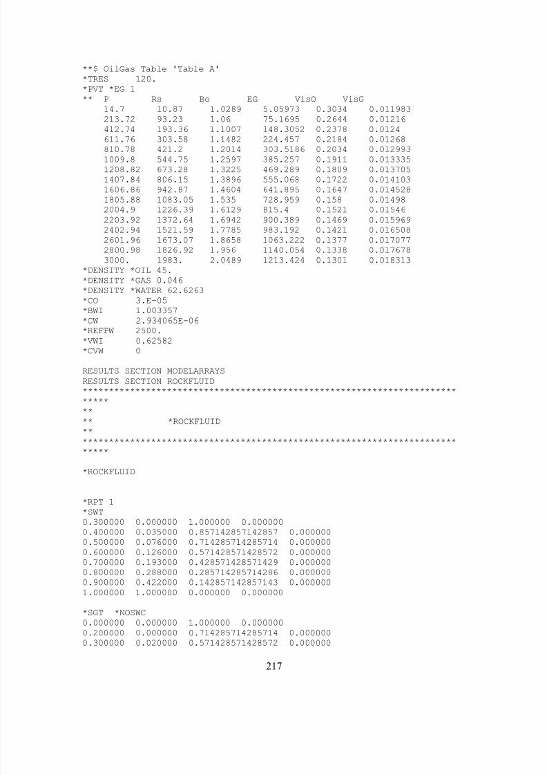
7/23/2019 Armenta Dis
http://slidepdf.com/reader/full/armenta-dis 235/263
**$ OilGas Table 'Table A'*TRES 120.*PVT *EG 1** P Rs Bo EG VisO VisG
14.7 10.87 1.0289 5.05973 0.3034 0.011983213.72 93.23 1.06 75.1695 0.2644 0.01216412.74 193.36 1.1007 148.3052 0.2378 0.0124611.76 303.58 1.1482 224.457 0.2184 0.01268810.78 421.2 1.2014 303.5186 0.2034 0.0129931009.8 544.75 1.2597 385.257 0.1911 0.0133351208.82 673.28 1.3225 469.289 0.1809 0.0137051407.84 806.15 1.3896 555.068 0.1722 0.0141031606.86 942.87 1.4604 641.895 0.1647 0.0145281805.88 1083.05 1.535 728.959 0.158 0.014982004.9 1226.39 1.6129 815.4 0.1521 0.015462203.92 1372.64 1.6942 900.389 0.1469 0.0159692402.94 1521.59 1.7785 983.192 0.1421 0.0165082601.96 1673.07 1.8658 1063.222 0.1377 0.0170772800.98 1826.92 1.956 1140.054 0.1338 0.0176783000. 1983. 2.0489 1213.424 0.1301 0.018313
*DENSITY *OIL 45.*DENSITY *GAS 0.046*DENSITY *WATER 62.6263*CO 3.E-05*BWI 1.003357*CW 2.934065E-06*REFPW 2500.*VWI 0.62582*CVW 0
RESULTS SECTION MODELARRAYSRESULTS SECTION ROCKFLUID******************************************************************************** *ROCKFLUID******************************************************************************
*ROCKFLUID
*RPT 1*SWT0.300000 0.000000 1.000000 0.0000000.400000 0.035000 0.857142857142857 0.000000
0.500000 0.076000 0.714285714285714 0.0000000.600000 0.126000 0.571428571428572 0.0000000.700000 0.193000 0.428571428571429 0.0000000.800000 0.288000 0.285714285714286 0.0000000.900000 0.422000 0.142857142857143 0.0000001.000000 1.000000 0.000000 0.000000
*SGT *NOSWC0.000000 0.000000 1.000000 0.0000000.200000 0.000000 0.714285714285714 0.0000000.300000 0.020000 0.571428571428572 0.000000
217

7/23/2019 Armenta Dis
http://slidepdf.com/reader/full/armenta-dis 236/263
0.400000 0.081000 0.428571428571429 0.0000000.500000 0.183000 0.285714285714286 0.0000000.600000 0.325000 0.142857142857143 0.0000000.700000 0.900000 0.000000 0.000000
*NONDARCY *FG1*KROIL *SEGREGATED
RESULTS SECTION ROCKARRAYSRESULTS SECTION INIT******************************************************************************** *INITIAL*******************************************************************************INITIAL**------------------------------------------------------------
**SS-NOEFFECT** RPTSOL** 6* 2 2 /** -------------------------------------------------------------**SS-ENDNOEFFECT**------------------------------------------------------------*VERTICAL *DEPTH_AVE *WATER_GAS *TRANZONE *EQUIL**$ Data for PVT Region 1**$ -------------------------------------*REFDEPTH 5000.*REFPRES 2300.*DWGC 5100.
RESULTS SECTION INITARRAYS
**$ RESULTS PROP PB Units: psi**$ RESULTS PROP Minimum Value: 0 Maximum Value: 0PB CON 0RESULTS SECTION NUMERICAL*NUMERICAL
RESULTS SECTION NUMARRAYSRESULTS SECTION GBKEYWORDSRUN
**SS-UNKNOWN** RPTRST** 4 / RESTARTS ONCE A YEAR**SS-ENDUNKNOWN
DATE 2002 01 01.
**------------------------------------------------------------
218

7/23/2019 Armenta Dis
http://slidepdf.com/reader/full/armenta-dis 237/263
**SS-NOEFFECT** NOECHO**SS-ENDNOEFFECT**------------------------------------------------------------PTUBE WATER_GAS 1DEPTH 5000.QG5.E+05 1.E+06 3.E+06 5.E+06 1.E+07 1.5E+07 1.8E+07WGR0 5.E-05 1.E-04 0.0002 0.0004 0.0006 0.0008 0.001WHP300. 500. 700.BHPTG
1 1 3.37024000E+02 5.59849000E+02 7.84870000E+022 1 1.00767000E+03 1.33083000E+03 1.63681000E+033 1 1.02840000E+03 1.35532000E+03 1.66413000E+034 1 1.06877000E+03 1.40292000E+03 1.71647000E+035 1 1.14745000E+03 1.49259000E+03 1.81241000E+036 1 1.22282000E+03 1.57486000E+03 1.89758000E+037 1 1.29426000E+03 1.65009000E+03 1.97324000E+03
8 1 1.36153000E+03 1.71853000E+03 2.04060000E+031 2 3.45916000E+02 5.65127000E+02 7.88564000E+022 2 6.85715000E+02 1.14235000E+03 1.43549000E+033 2 7.98357000E+02 1.17999000E+03 1.46993000E+034 2 9.06174000E+02 1.23965000E+03 1.53687000E+035 2 1.03248000E+03 1.35495000E+03 1.66240000E+036 2 1.13624000E+03 1.46356000E+03 1.77592000E+037 2 1.23434000E+03 1.56415000E+03 1.87771000E+038 2 1.32752000E+03 1.65684000E+03 1.96914000E+031 3 4.25316000E+02 6.15848000E+02 8.24883000E+022 3 5.26979000E+02 7.95789000E+02 1.08259000E+033 3 6.46858000E+02 9.33680000E+02 1.24089000E+034 3 8.40372000E+02 1.14544000E+03 1.43807000E+035 3 1.14282000E+03 1.42442000E+03 1.68147000E+036 3 1.39809000E+03 1.65458000E+03 1.89757000E+037 3 1.62877000E+03 1.86048000E+03 2.09286000E+038 3 1.83827000E+03 2.04934000E+03 2.27214000E+031 4 5.47796000E+02 7.04360000E+02 8.91575000E+022 4 6.66316000E+02 8.23118000E+02 1.05816000E+033 4 7.92196000E+02 9.70272000E+02 1.22716000E+034 4 1.03062000E+03 1.22814000E+03 1.50399000E+035 4 1.50309000E+03 1.68890000E+03 1.92590000E+036 4 1.90174000E+03 2.07013000E+03 2.26855000E+03
7 4 2.24629000E+03 2.39607000E+03 2.57229000E+038 4 2.56051000E+03 2.69480000E+03 2.85658000E+031 5 9.16800000E+02 1.01422000E+03 1.14823000E+03
2 5 1.17821000E+03 1.26153000E+03 1.38041000E+033 5 1.40325000E+03 1.48036000E+03 1.59380000E+034 5 1.79136000E+03 1.87547000E+03 2.00566000E+035 5 2.63140000E+03 2.70978000E+03 2.82769000E+036 5 3.33657000E+03 3.40719000E+03 3.51185000E+037 5 3.93384000E+03 4.00224000E+03 4.09229000E+038 5 4.54574000E+03 4.60380000E+03 4.68526000E+031 6 1.30649000E+03 1.37324000E+03 1.47144000E+032 6 1.69683000E+03 1.75038000E+03 1.83132000E+033 6 2.01561000E+03 2.06380000E+03 2.13846000E+034 6 2.60038000E+03 2.65034000E+03 2.72983000E+03
219

7/23/2019 Armenta Dis
http://slidepdf.com/reader/full/armenta-dis 238/263
5 6 3.81908000E+03 3.86469000E+03 3.93860000E+036 6 4.76408000E+03 4.80311000E+03 4.86696000E+037 6 5.78065000E+03 5.81806000E+03 5.87715000E+038 6 6.91460000E+03 6.95034000E+03 7.00651000E+031 7 1.53942000E+03 1.59511000E+03 1.67903000E+032 7 2.00157000E+03 2.04461000E+03 2.11135000E+033 7 2.37484000E+03 2.41335000E+03 2.47443000E+034 7 3.08950000E+03 3.12890000E+03 3.19348000E+035 7 4.60402000E+03 4.64024000E+03 4.70113000E+036 7 5.69293000E+03 5.72329000E+03 5.77622000E+037 7 7.03960000E+03 7.06884000E+03 7.11864000E+038 7 8.57618000E+03 8.60434000E+03 8.65223000E+03
GROUP 'G' ATTACHTO 'FIELD'
WELL 1 'P' ATTACHTO 'G'PRODUCER 'P'PWELLBORE TABLE 5000. 1OPERATE MAX STW 3000. CONT
OPERATE MIN WHP IMPLICIT 300. CONTOPERATE MIN BHP 14.7 CONTMONITOR MAX WGR 1. STOPMONITOR MIN STG 0 STOP
GEOMETRY K 0.333 0.37 1. 0.PERF GEO 'P'
1 1 1 1. OPEN1 1 2 1. OPEN1 1 3 1. OPEN1 1 4 1. OPEN1 1 5 1. OPEN1 1 6 1. OPEN1 1 7 1. OPEN1 1 8 1. OPEN1 1 9 1. OPEN1 1 10 1. OPEN1 1 11 1. OPEN1 1 12 1. OPEN1 1 13 1. OPEN1 1 14 1. OPEN1 1 15 1. OPEN1 1 16 1. OPEN1 1 17 1. OPEN1 1 18 1. OPEN1 1 19 1. OPEN1 1 20 1. OPEN
1 1 21 1. OPEN1 1 22 1. OPEN1 1 23 1. OPEN1 1 24 1. OPEN1 1 25 1. OPEN
XFLOW-MODEL 'P' FULLY-MIXED
OPEN 'P'
TIME 30.4
220

7/23/2019 Armenta Dis
http://slidepdf.com/reader/full/armenta-dis 239/263
TIME 60.8
TIME 91.2
TIME 121.6
TIME 152
TIME 182.4
TIME 212.8
TIME 243.2
TIME 273.6
TIME 304
TIME 334.4
TIME 364.8
TIME 395.2
TIME 425.6
TIME 456
TIME 486.4
TIME 516.8
TIME 547.2
TIME 577.6
TIME 608
TIME 638.4
TIME 668.8
TIME 699.2
TIME 729.6
TIME 760
TIME 790.4
TIME 820.8
TIME 851.2
TIME 881.6
TIME 912
221

7/23/2019 Armenta Dis
http://slidepdf.com/reader/full/armenta-dis 240/263
TIME 942.4
TIME 972.8
TIME 1003.2
TIME 1033.6
TIME 1064
TIME 1094.4
TIME 1124.8
TIME 1155.2
TIME 1185.6
TIME 1216
TIME 1246.4
TIME 1276.8
TIME 1307.2
TIME 1337.6
TIME 1368
TIME 1398.4
TIME 1428.8
TIME 1459.2
TIME 1489.6
TIME 1520
TIME 1550.4
TIME 1580.8
TIME 1611.2
TIME 1641.6
TIME 1672
TIME 1702.4
TIME 1732.8
TIME 1763.2
TIME 1793.6
222

7/23/2019 Armenta Dis
http://slidepdf.com/reader/full/armenta-dis 241/263
TIME 1824
TIME 1854.4
TIME 1884.8
TIME 1915.2
TIME 1945.6
TIME 1976
TIME 2006.4
TIME 2036.8
TIME 2067.2
TIME 2097.6
TIME 2128
TIME 2158.4
TIME 2188.8
TIME 2219.2
TIME 2249.6
TIME 2280
TIME 2310.4
TIME 2340.8
TIME 2371.2
TIME 2401.6
TIME 2432
TIME 2462.4
TIME 2492.8
TIME 2523.2
TIME 2553.6
TIME 2584
TIME 2614.4
TIME 2644.8
TIME 2675.2
223

7/23/2019 Armenta Dis
http://slidepdf.com/reader/full/armenta-dis 242/263
TIME 2705.6
TIME 2736
TIME 2766.4
TIME 2796.8
TIME 2827.2
TIME 2857.6
TIME 2888
TIME 2918.4
TIME 2948.8
TIME 2979.2
TIME 3009.6
TIME 3040
TIME 3070.4
TIME 3100.8
TIME 3131.2
TIME 3161.6
TIME 3192
TIME 3222.4
TIME 3252.8
TIME 3283.2
TIME 3313.6
TIME 3344
TIME 3374.4
TIME 3404.8
TIME 3435.2
TIME 3465.6
TIME 3496
TIME 3526.4
TIME 3556.8
224

7/23/2019 Armenta Dis
http://slidepdf.com/reader/full/armenta-dis 243/263
TIME 3587.2
TIME 3617.6
TIME 3648
TIME 3678.4
TIME 3708.8
TIME 3739.2
TIME 3769.6
TIME 3800
TIME 3830.4
TIME 3860.8
TIME 3891.2
TIME 3921.6
TIME 3952
TIME 3982.4
TIME 4012.8
TIME 4043.2
TIME 4073.6
TIME 4104
TIME 4134.4
TIME 4164.8
TIME 4195.2
TIME 4225.6
TIME 4256
TIME 4286.4
TIME 4316.8
TIME 4347.2
TIME 4377.6
TIME 4408
TIME 4438.4
225

7/23/2019 Armenta Dis
http://slidepdf.com/reader/full/armenta-dis 244/263
226
TIME 4468.8
TIME 4499.2
TIME 4529.6
TIME 4560
TIME 4590.4
TIME 4620.8
TIME 4651.2
TIME 4681.6
TIME 4712
TIME 4742.4
TIME 4772.8
TIME 4803.2
STOP***************************** TERMINATE SIMULATION*****************************
RESULTS SECTION WELLDATARESULTS SECTION PERFS

7/23/2019 Armenta Dis
http://slidepdf.com/reader/full/armenta-dis 245/263
APPENDIX F
EXAMPLE ECLIPSE DATA DECK FOR COMPARISON OF CONVENTIONAL
WELLS AND DWS WELLS
Runspec
Title
Effect of Completion Length on Conventional Wells
--Normal Reservoir Pressure (2300 psia), Horizontal Permeability 10 md,
--Length of Perforations: 20 ft.
MESSAGES
6* 3*5000 /
Radial
Dimens
-- NR Theta NZ
26 1 110 /
Gas
Water
Field
Regdims2 /
Welldims
-- Wells Con
1 100 /
VFPPDIMS
10 10 10 10 0 1 /
Start
1 'Jan' 2002 /
Nstack
100 /
Unifout
-------------------------------------------------------------
Grid
Tops
26*5000 /
Inrad
0.333 /
DRV
0.4170 0.3016 0.4229 0.5929 0.8313 1.166
1.634 2.292 3.213 4.505 6.317 8.857
12.42 17.41 24.41 34.23 48.00 67.30
94.36 132.3 185.5 260.1 364.7 511.4
717.0 2500 /
DZ
2600*1
234*10
26*1410/
Equals
'DTHETA' 360 /
'PERMR' 10 /
'PERMTHT' 10 /
'PERMZ' 5 /
'PORO' 0.25 /
'PORO' 0 26 26 1 1 1 100 /
'PORO' 10 26 26 1 1 101 110 /
/
227

7/23/2019 Armenta Dis
http://slidepdf.com/reader/full/armenta-dis 246/263
INIT
--RPTGRID
--1 /
-------------------------------------------------------------
PROPS
DENSITY
45 64 0.046 /
ROCK
2500 10E-6 /
PVTW
2500 1 2.6E-6 0.68 0 /
PVZG
-- Temperature
120 /
-- Press Z Visc
100 0.989 0.0122
300 0.967 0.0124
500 0.947 0.0126
700 0.927 0.0129
900 0.908 0.0133
1100 0.891 0.01371300 0.876 0.0141
1500 0.863 0.0146
1700 0.853 0.0151
1900 0.845 0.0157
2100 0.840 0.0163
2300 0.837 0.0167
2500 0.837 0.0177
2700 0.839 0.0184
3200 0.844 0.0202
/
--Saturation Functions
--Sgc = 0.20
--Krg @ Swir = 0.9
--Swir = 0.3
--Sorg = 0.0
SGFN
--Using Honarpour Equation 71
-- Sg Krg Pc
0.00 0.000 0.0
0.20 0.000 0.0
0.30 0.020 0.0
0.40 0.081 0.0
0.50 0.183 0.0
0.60 0.325 0.0
0.70 0.900 0.0
/
SWFN--Using Honarpour Equation 67
-- Sw Krw Pc
0.3 0.000 0.0
0.4 0.035 0.0
0.5 0.076 0.0
0.6 0.126 0.0
0.7 0.193 0.0
0.8 0.288 0.0
0.9 0.422 0.0
1.0 1.000 0.0
228

7/23/2019 Armenta Dis
http://slidepdf.com/reader/full/armenta-dis 247/263
/
-------------------------------------------------------------
REGIONS
Fipnum
2600*1
260*2
/
-------------------------------------------------------------
SOLUTION
EQUIL
5000 2300 5100 0 5100 0 /
RPTSOL
6* 2 2 /
-------------------------------------------------------------
SUMMARY
SEPARATE
RPTONLY
WGPR
/
WWPR
/WBHP
/
WTHP
/
WGPT
/
WWPT
/
WBP
/
RGIP
/
RPR
1 2 /
TCPU
-------------------------------------------------------------
SCHEDULE
NOECHO
INCLUDE
'WELL-5000-VI.VFP' /
ECHO
RPTSCHED
6* 2 /
RPTRST
4 / restarts once a year
TUNING
0.0007 30.4 0.0007 0.0007 1.2 /3* 0.00001 3* 0.0001 /
2* 500 1* 50 /
WELSPECS
'P' 'G' 1 1 5000 'GAS' 2* 'STOP' 'YES' /
/
COMPDAT
'P' 1 1 1 20 'OPEN' 2* 0.666 /
/
WCONPROD
'P' 'OPEN' 'THP' 1* 3000 40000 3* 300 1 /
229

7/23/2019 Armenta Dis
http://slidepdf.com/reader/full/armenta-dis 248/263
/
WECON
'P' 4* 1.0 'WELL' 'YES' /
/
TSTEP
48*30.4 /
TSTEP
48*30.4 /
TSTEP
48*30.4 /
TSTEP
48*30.4 /
TSTEP
48*30.4 /
TSTEP
48*30.4 /
TSTEP
48*30.4 /
TSTEP
48*30.4 /
TSTEP48*30.4 /
TSTEP
48*30.4 /
TSTEP
48*30.4 /
TSTEP
48*30.4 /
TSTEP
48*30.4 /
TSTEP
48*30.4 /
TSTEP
48*30.4 /
TSTEP
48*30.4 /
TSTEP
48*30.4 /
TSTEP
48*30.4 /
TSTEP
48*30.4 /
TSTEP
48*30.4 /
TSTEP
48*30.4 /
TSTEP
48*30.4 /End
230

7/23/2019 Armenta Dis
http://slidepdf.com/reader/full/armenta-dis 249/263
EXAMPLE ECLIPSE DATA DECK FOR COMPARISON OF DWS AND DGWS
DWS MODEL
Runspec
Title
Comparison of DWS and DGWS
--DWS-2 Model: Top completion 70 ft; Bottom Completion 60 ft
MESSAGES
6* 3*5000 /
Radial
Dimens
-- NR Theta NZ
26 1 110 /
Gas
Water
Field
Regdims
2 /Welldims
-- Wells Con Group Well in group
2 100 1 2 /
VFPPDIMS
10 10 10 10 0 2 /
Start
1 'Jan' 2002 /
Nstack
300 /
Unifout
-------------------------------------------------------------
Grid
Tops
26*5000 /
Inrad
0.333 /
DRV
0.4170 0.3016 0.4229 0.5929 0.8313 1.166
1.634 2.292 3.213 4.505 6.317 8.857
12.42 17.41 24.41 34.23 48.00 67.30
94.36 132.3 185.5 260.1 364.7 511.4
717.0 2500 /
DZ
2600*1
234*10
26*1410
/Equals
'DTHETA' 360 /
'PERMR' 1 /
'PERMTHT' 1 /
'PERMZ' .5 /
'PORO' 0.25 /
'PORO' 0 26 26 1 1 1 100 /
'PORO' 10 26 26 1 1 101 110 /
/
INIT
231

7/23/2019 Armenta Dis
http://slidepdf.com/reader/full/armenta-dis 250/263
--RPTGRID
--1 /
-------------------------------------------------------------
PROPS
DENSITY
45 64 0.046 /
ROCK
2500 10E-6 /
PVTW
2500 1 2.6E-6 0.68 0 /
PVZG
-- Temperature
120 /
-- Press Z Visc
100 0.989 0.0122
300 0.967 0.0124
500 0.947 0.0126
700 0.927 0.0129
900 0.908 0.0133
1100 0.891 0.0137
1300 0.876 0.01411500 0.863 0.0146
1700 0.853 0.0151
1900 0.845 0.0157
2100 0.840 0.0163
2300 0.837 0.0167
2500 0.837 0.0177
2700 0.839 0.0184
3200 0.844 0.0202
/
SGFN
--Using Honarpour Equation 71
-- Sg Krg Pc
0.00 0.000 0.0
0.20 0.000 0.0
0.30 0.020 0.0
0.40 0.081 0.0
0.50 0.183 0.0
0.60 0.325 0.0
0.70 0.900 0.0
/
SWFN
--Using Honarpour Equation 67
-- Sw Krw Pc
0.3 0.000 0.0
0.4 0.035 0.0
0.5 0.076 0.00.6 0.126 0.0
0.7 0.193 0.0
0.8 0.288 0.0
0.9 0.422 0.0
1.0 1.000 0.0
/
-------------------------------------------------------------
REGIONS
Fipnum
2600*1
232

7/23/2019 Armenta Dis
http://slidepdf.com/reader/full/armenta-dis 251/263
260*2
/
-------------------------------------------------------------
SOLUTION
EQUIL
5000 1500 5100 0 5100 0 /
RPTSOL
6* 2 2 /
-------------------------------------------------------------
SUMMARY
SEPARATE
RPTONLY
WGPR
/
WWPR
/
WBHP
/
WTHP
/
WGPT/
WWPT
/
WBP
/
RGIP
/
RPR
1 2 /
TCPU
-------------------------------------------------------------
SCHEDULE
NOECHO
INCLUDE
'WELL-5000-DGWS.VFP' /
ECHO
RPTSCHED
6* 2 /
RPTRST
4 / restarts once a year
TUNING
0.0007 30.4 0.0007 0.0007 1.2 /
3* 0.00001 3* 0.0001 /
2* 500 1* 100 /
WELSPECS
'P' 'G' 1 1 5000 'GAS' 2* 'STOP' 'YES' /
'W' 'G' 1 1 5100 'WATER' 2* 'STOP' 'YES' //
COMPDAT
'P' 1 1 1 70 'OPEN' 2* 0.666 /
'W' 1 1 71 103 'OPEN' 2* 0.666 /
/
WCONPROD
'P' 'OPEN' 'THP' 6* 300 1 /
'W' 'OPEN' 'THP' 6* 300 2 /
/
WECON
233

7/23/2019 Armenta Dis
http://slidepdf.com/reader/full/armenta-dis 252/263
'P' 1* 400 3* 'WELL' 'YES' /
/
TSTEP
35*30.4 /
TSTEP
48*30.4 /
TSTEP
48*30.4 /
/
WCONPROD
'W' 'OPEN' 'THP' 6* 14.7 2 /
/
TSTEP
48*30.4 /
TSTEP
48*30.4 /
TSTEP
48*30.4 /
TSTEP
48*30.4 /
TSTEP48*30.4 /
TSTEP
48*30.4 /
TSTEP
48*30.4 /
TSTEP
48*30.4 /
TSTEP
48*30.4 /
TSTEP
48*30.4 /
TSTEP
48*30.4 /
TSTEP
48*30.4 /
TSTEP
48*30.4 /
TSTEP
48*30.4 /
TSTEP
48*30.4 /
TSTEP
48*30.4 /
TSTEP
48*30.4 /
TSTEP
48*30.4 /TSTEP
48*30.4 /
TSTEP
48*30.4 /
TSTEP
48*30.4 /
TSTEP
48*30.4 /
TSTEP
48*30.4 /
234

7/23/2019 Armenta Dis
http://slidepdf.com/reader/full/armenta-dis 253/263
TSTEP
48*30.4 /
TSTEP
48*30.4 /
TSTEP
48*30.4 /
TSTEP
48*30.4 /
TSTEP
48*30.4 /
TSTEP
48*30.4 /
TSTEP
48*30.4 /
TSTEP
48*30.4 /
TSTEP
48*30.4 /
TSTEP
48*30.4 /
TSTEP48*30.4 /
TSTEP
48*30.4 /
TSTEP
48*30.4 /
TSTEP
48*30.4 /
TSTEP
48*30.4 /
TSTEP
48*30.4 /
TSTEP
48*30.4 /
TSTEP
48*30.4 /
TSTEP
48*30.4 /
TSTEP
48*30.4 /
TSTEP
48*30.4 /
TSTEP
48*30.4 /
TSTEP
48*30.4 /
TSTEP
48*30.4 /TSTEP
48*30.4 /
TSTEP
48*30.4 /
TSTEP
48*30.4 /
TSTEP
48*30.4 /
TSTEP
48*30.4 /
235
7/23/2019 Armenta Dis
http://slidepdf.com/reader/full/armenta-dis 254/263
TSTEP
48*30.4 /
TSTEP
48*30.4 /
TSTEP
48*30.4 /
TSTEP
48*30.4 /
TSTEP
48*30.4 /
TSTEP
48*30.4 /
End
236
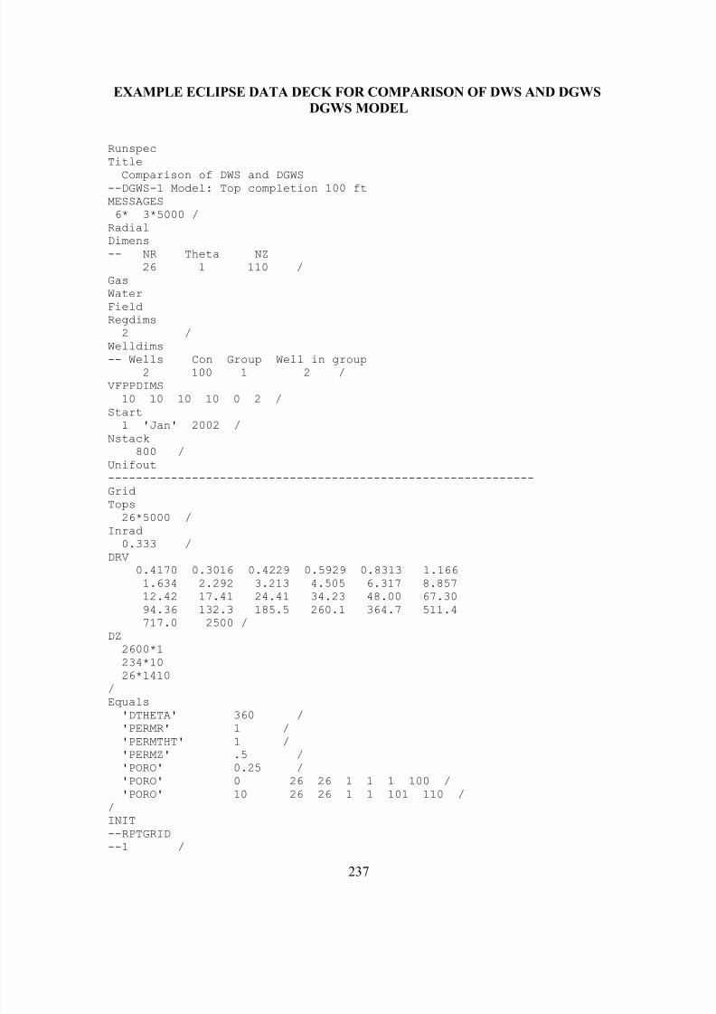
7/23/2019 Armenta Dis
http://slidepdf.com/reader/full/armenta-dis 255/263
EXAMPLE ECLIPSE DATA DECK FOR COMPARISON OF DWS AND DGWS
DGWS MODEL
Runspec
Title
Comparison of DWS and DGWS--DGWS-1 Model: Top completion 100 ft
MESSAGES
6* 3*5000 /
Radial
Dimens
-- NR Theta NZ
26 1 110 /
Gas
Water
Field
Regdims
2 /
Welldims
-- Wells Con Group Well in group
2 100 1 2 /
VFPPDIMS
10 10 10 10 0 2 /
Start
1 'Jan' 2002 /
Nstack
800 /
Unifout
-------------------------------------------------------------
Grid
Tops
26*5000 /
Inrad0.333 /
DRV
0.4170 0.3016 0.4229 0.5929 0.8313 1.166
1.634 2.292 3.213 4.505 6.317 8.857
12.42 17.41 24.41 34.23 48.00 67.30
94.36 132.3 185.5 260.1 364.7 511.4
717.0 2500 /
DZ
2600*1
234*10
26*1410
/
Equals
'DTHETA' 360 /
'PERMR' 1 /
'PERMTHT' 1 /
'PERMZ' .5 /
'PORO' 0.25 /
'PORO' 0 26 26 1 1 1 100 /
'PORO' 10 26 26 1 1 101 110 /
/
INIT
--RPTGRID
--1 /
237
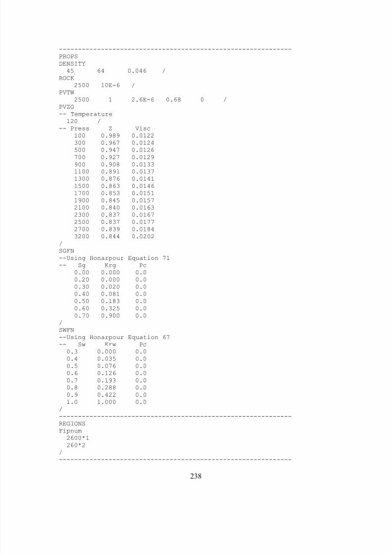
7/23/2019 Armenta Dis
http://slidepdf.com/reader/full/armenta-dis 256/263
-------------------------------------------------------------
PROPS
DENSITY
45 64 0.046 /
ROCK
2500 10E-6 /
PVTW
2500 1 2.6E-6 0.68 0 /
PVZG
-- Temperature
120 /
-- Press Z Visc
100 0.989 0.0122
300 0.967 0.0124
500 0.947 0.0126
700 0.927 0.0129
900 0.908 0.0133
1100 0.891 0.0137
1300 0.876 0.0141
1500 0.863 0.0146
1700 0.853 0.01511900 0.845 0.0157
2100 0.840 0.0163
2300 0.837 0.0167
2500 0.837 0.0177
2700 0.839 0.0184
3200 0.844 0.0202
/
SGFN
--Using Honarpour Equation 71
-- Sg Krg Pc
0.00 0.000 0.0
0.20 0.000 0.0
0.30 0.020 0.0
0.40 0.081 0.0
0.50 0.183 0.0
0.60 0.325 0.0
0.70 0.900 0.0
/
SWFN
--Using Honarpour Equation 67
-- Sw Krw Pc
0.3 0.000 0.0
0.4 0.035 0.0
0.5 0.076 0.0
0.6 0.126 0.0
0.7 0.193 0.0
0.8 0.288 0.00.9 0.422 0.0
1.0 1.000 0.0
/
-------------------------------------------------------------
REGIONS
Fipnum
2600*1
260*2
/
-------------------------------------------------------------
238

7/23/2019 Armenta Dis
http://slidepdf.com/reader/full/armenta-dis 257/263
SOLUTION
EQUIL
5000 1500 5100 0 5100 0 /
RPTSOL
6* 2 2 /
-------------------------------------------------------------
SUMMARY
SEPARATE
RPTONLY
WGPR
/
WWPR
/
WBHP
/
WTHP
/
WGPT
/
WWPT
/WBP
/
RGIP
/
RPR
1 2 /
TCPU
-------------------------------------------------------------
SCHEDULE
NOECHO
INCLUDE
'WELL-5000-DGWS.VFP' /
ECHO
RPTSCHED
6* 2 /
RPTRST
4 / restarts once a year
TUNING
0.0007 30.4 0.0007 0.0007 1.2 /
3* 0.00001 3* 0.0001 /
2* 1000 1* 500 /
WELSPECS
'P' 'G' 1 1 5000 'GAS' 2* 'STOP' 'YES' /
'W' 'G' 1 1 5000 'WATER' 2* 'STOP' 'YES' /
/
COMPDAT
'P' 1 1 1 100 'OPEN' 2* 0.666 /'W' 1 1 1 100 'SHUT' 2* 0.666 /
/
WCONPROD
'P' 'OPEN' 'THP' 1* 3000 40000 2* 50 300 1 /
'W' 'SHUT' 'THP' 6* 300 2 /
/
WECON
'P' 1* 400 3* 'WELL' 'YES' /
/
TSTEP
239

7/23/2019 Armenta Dis
http://slidepdf.com/reader/full/armenta-dis 258/263
48*30.4 /
TSTEP
31*30.4 /
/
COMPDAT
'W' 1 1 1 100 'OPEN' 2* 0.666 /
/
WCONPROD
'W' 'OPEN' 'THP' 6* 300 2 /
'P' 'SHUT' 'THP' 6* 300 1 /
/
TSTEP
48*30.4 /
TSTEP
48*30.4 /
TSTEP
48*30.4 /
TSTEP
48*30.4 /
TSTEP48*30.4 /
TSTEP
48*30.4 /
TSTEP
48*30.4 /
TSTEP
48*30.4 /
TSTEP
48*30.4 /
TSTEP
48*30.4 /
TSTEP
48*30.4 /
TSTEP
48*30.4 /
TSTEP
48*30.4 /
TSTEP
48*30.4 /
TSTEP
48*30.4 /
TSTEP
48*30.4 /
TSTEP
48*30.4 /
TSTEP
48*30.4 /TSTEP
48*30.4 /
TSTEP
48*30.4 /
TSTEP
48*30.4 /
TSTEP
48*30.4 /
TSTEP
48*30.4 /
240

7/23/2019 Armenta Dis
http://slidepdf.com/reader/full/armenta-dis 259/263
TSTEP
48*30.4 /
TSTEP
48*30.4 /
TSTEP
48*30.4 /
TSTEP
48*30.4 /
TSTEP
48*30.4 /
TSTEP
48*30.4 /
TSTEP
48*30.4 /
TSTEP
48*30.4 /
TSTEP
48*30.4 /
TSTEP
48*30.4 /
TSTEP48*30.4 /
TSTEP
48*30.4 /
TSTEP
48*30.4 /
TSTEP
48*30.4 /
TSTEP
48*30.4 /
TSTEP
48*30.4 /
TSTEP
48*30.4 /
TSTEP
48*30.4 /
TSTEP
48*30.4 /
TSTEP
48*30.4 /
TSTEP
48*30.4 /
TSTEP
48*30.4 /
TSTEP
48*30.4 /
TSTEP
48*30.4 /TSTEP
48*30.4 /
TSTEP
48*30.4 /
TSTEP
48*30.4 /
TSTEP
48*30.4 /
TSTEP
48*30.4 /
241

7/23/2019 Armenta Dis
http://slidepdf.com/reader/full/armenta-dis 260/263
TSTEP
48*30.4 /
TSTEP
48*30.4 /
TSTEP
48*30.4 /
TSTEP
48*30.4 /
TSTEP
48*30.4 /
TSTEP
48*30.4 /
End
242

7/23/2019 Armenta Dis
http://slidepdf.com/reader/full/armenta-dis 261/263
ECLIPSE VFP INCLUDED FILE: WELL-5000-DGWS
VFPPROD
1 5.00000E+003 'GAS' 'WGR' 'OGR' 'THP' '' 'FIELD' 'BHP'/
5.00000E+002 1.00000E+003 3.00000E+003 5.00000E+003
1.00000E+004 1.50000E+004 1.80000E+004 /
3.00000E+002 5.00000E+002 7.00000E+002 /
0.00000E+000 5.00000E-002 1.00000E-001 2.00000E-001
4.00000E-001 6.00000E-001 8.00000E-001 1.00000E+000 /
0.00000E+000 /
0.00000E+000 /
1 1 1 1 3.37024E+002 3.45916E+002 4.25316E+002 5.47796E+002
9.16800E+002 1.30649E+003 1.53942E+003 /
2 1 1 1 5.59849E+002 5.65127E+002 6.15848E+002 7.04360E+002
1.01422E+003 1.37324E+003 1.59511E+003 /
3 1 1 1 7.84870E+002 7.88564E+002 8.24884E+002 8.91574E+002
1.14823E+003 1.47144E+003 1.67903E+003 /
1 2 1 1 1.00767E+003 6.85715E+002 5.26979E+002 6.66317E+0021.17821E+003 1.69683E+003 2.00157E+003 /
2 2 1 1 1.33083E+003 1.14235E+003 7.95789E+002 8.23119E+002
1.26153E+003 1.75038E+003 2.04461E+003 /
3 2 1 1 1.63681E+003 1.43549E+003 1.08259E+003 1.05816E+003
1.38041E+003 1.83132E+003 2.11135E+003 /
1 3 1 1 1.02840E+003 7.98358E+002 6.46858E+002 7.92196E+002
1.40325E+003 2.01561E+003 2.37484E+003 /
2 3 1 1 1.35532E+003 1.17999E+003 9.33680E+002 9.70272E+002
1.48036E+003 2.06380E+003 2.41335E+003 /
3 3 1 1 1.66413E+003 1.46993E+003 1.24089E+003 1.22716E+003
1.59380E+003 2.13846E+003 2.47443E+003 /
1 4 1 1 1.06877E+003 9.06174E+002 8.40372E+002 1.03062E+003
1.79136E+003 2.60038E+003 3.08950E+003 /2 4 1 1 1.40292E+003 1.23965E+003 1.14544E+003 1.22814E+003
1.87547E+003 2.65034E+003 3.12890E+003 /
3 4 1 1 1.71647E+003 1.53687E+003 1.43807E+003 1.50399E+003
2.00566E+003 2.72983E+003 3.19348E+003 /
1 5 1 1 1.14745E+003 1.03248E+003 1.14282E+003 1.50309E+003
2.63140E+003 3.81908E+003 4.60402E+003 /
2 5 1 1 1.49259E+003 1.35495E+003 1.42442E+003 1.68890E+003
2.70978E+003 3.86469E+003 4.64024E+003 /
3 5 1 1 1.81241E+003 1.66240E+003 1.68147E+003 1.92590E+003
2.82769E+003 3.93860E+003 4.70113E+003 /
1 6 1 1 1.22282E+003 1.13624E+003 1.39809E+003 1.90174E+003
3.33657E+003 4.76408E+003 5.69293E+003 /
2 6 1 1 1.57486E+003 1.46356E+003 1.65458E+003 2.07013E+003
3.40719E+003 4.80311E+003 5.72329E+003 /3 6 1 1 1.89758E+003 1.77592E+003 1.89757E+003 2.26855E+003
3.51185E+003 4.86696E+003 5.77621E+003 /
1 7 1 1 1.29426E+003 1.23434E+003 1.62877E+003 2.24629E+003
3.93384E+003 5.78065E+003 7.03960E+003 /
2 7 1 1 1.65009E+003 1.56415E+003 1.86048E+003 2.39607E+003
4.00224E+003 5.81806E+003 7.06883E+003 /
3 7 1 1 1.97324E+003 1.87771E+003 2.09286E+003 2.57229E+003
4.09229E+003 5.87715E+003 7.11864E+003 /
1 8 1 1 1.36153E+003 1.32752E+003 1.83827E+003 2.56051E+003
4.54574E+003 6.91460E+003 8.57619E+003 /
243

7/23/2019 Armenta Dis
http://slidepdf.com/reader/full/armenta-dis 262/263
244
2 8 1 1 1.71853E+003 1.65684E+003 2.04934E+003 2.69480E+003
4.60380E+003 6.95034E+003 8.60433E+003 /
3 8 1 1 2.04060E+003 1.96914E+003 2.27214E+003 2.85658E+003
4.68526E+003 7.00651E+003 8.65222E+003 /
VFPPROD
2 5.00000E+003 'GAS' 'WGR' 'OGR' 'THP' '' 'FIELD' 'BHP'/
5.00000E+002 1.00000E+003 3.00000E+003 5.00000E+003
1.00000E+004 1.50000E+004 /
1.00000E+002 3.00000E+002 5.00000E+002 7.00000E+002 /
0.00000E+000 1.20000E+000 /
0.00000E+000 /
0.00000E+000 /
1 1 1 1 1.20764E+002 1.44218E+002 2.88734E+002 4.52423E+002
8.67338E+002 1.27581E+003 /
2 1 1 1 3.37024E+002 3.45916E+002 4.25316E+002 5.47796E+002
9.16800E+002 1.30649E+003 /
3 1 1 1 5.59849E+002 5.65127E+002 6.15848E+002 7.04360E+0021.01422E+003 1.37324E+003 /
4 1 1 1 7.84870E+002 7.88564E+002 8.24884E+002 8.91574E+002
1.14823E+003 1.47144E+003 /
1 2 1 1 1.20764E+002 1.44218E+002 2.88734E+002 4.52423E+002
8.67338E+002 1.27581E+003 /
2 2 1 1 3.37024E+002 3.45916E+002 4.25316E+002 5.47796E+002
9.16800E+002 1.30649E+003 /
3 2 1 1 5.59849E+002 5.65127E+002 6.15848E+002 7.04360E+002
1.01422E+003 1.37324E+003 /
4 2 1 1 7.84870E+002 7.88564E+002 8.24884E+002 8.91574E+002
1.14823E+003 1.47144E+003 /

7/23/2019 Armenta Dis
http://slidepdf.com/reader/full/armenta-dis 263/263
VITA
Miguel A. Armenta Sanchez, son of Miguel A. Armenta Van-Strahalen and