Arrow-Debreu Equilibrium

Econ 2100 Fall 2017

Lecture 22, November 16

Outline

1 Time and Uncertainty: dated events2 Uncertainty in General Equilibrium: Arrow-Debreu Economies

1 State-Contingent Commodities2 Preferences3 Production Sets4 Budget Sets

3 Arrow-Debreu Equilibrium

1 Examples

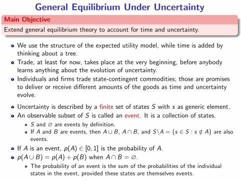
General Equilibrium Under UncertaintyMain ObjectiveExtend general equilibrium theory to account for time and uncertainty.

We use the structure of the expected utility model, while time is added bythinking about a tree.Trade, at least for now, takes place at the very beginning, before anybodylearns anything about the evolution of uncertainty.Individuals and firms trade state-contingent commodities; those are promisesto deliver or receive different amounts of the goods as time and uncertaintyevolve.

Uncertainty is described by a finite set of states S with s as generic element.An observable subset of S is called an event. It is a collection of states.

S and ∅ are events by definition.If A and B are events, then A ∪ B , A ∩ B , and S\A = {s ∈ S : s /∈ A} are alsoevents.

If A is an event, p(A) ∈ [0, 1] is the probability of A.p(A ∪ B) = p(A) + p(B) when A ∩ B = ∅.

The probability of an event is the sum of the probabilities of the individualstates in the event, provided these states are themselves events.

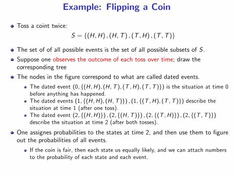
Example: Flipping a Coin

Toss a coint twice:

S = {(H,H) , (H,T ) , (T ,H) , (T ,T )}

The set of of all possible events is the set of all possible subsets of S .

Suppose one observes the outcome of each toss over time; draw thecorresponding tree

The nodes in the figure correspond to what are called dated events.

The dated event (0, {(H ,H), (H ,T ), (T ,H), (T ,T )}) is the situation at time 0before anything has happened.The dated events (1, {(H ,H), (H ,T )}) , (1, {(T ,H), (T ,T )}) describe thesituation at time 1 (after one toss).The dated event (2, {(H ,H)}) , (2, {(H ,T )}) , (2, {(T ,H)}) , (2, {(T ,T )})describe the situation at time 2 (after both tosses).

One assignes probabilities to the states at time 2, and then use them to figureout the probabilities of all events.

If the coin is fair, then each state us equally likely, and we can attach numbersto the probability of each state and each event.

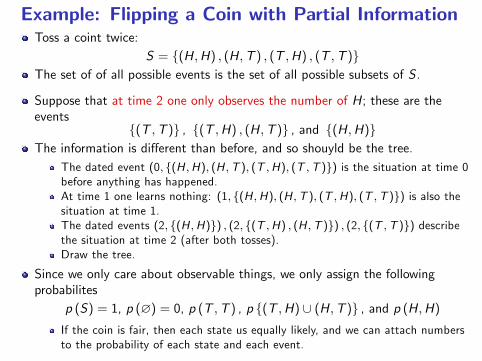
Example: Flipping a Coin with Partial InformationToss a coint twice:

S = {(H,H) , (H,T ) , (T ,H) , (T ,T )}The set of of all possible events is the set of all possible subsets of S .

Suppose that at time 2 one only observes the number of H; these are theevents

{(T ,T )} , {(T ,H) , (H,T )} , and {(H,H)}The information is different than before, and so shouyld be the tree.

The dated event (0, {(H ,H), (H ,T ), (T ,H), (T ,T )}) is the situation at time 0before anything has happened.At time 1 one learns nothing: (1, {(H ,H), (H ,T ), (T ,H), (T ,T )}) is also thesituation at time 1.The dated events (2, {(H ,H)}) , (2, {(T ,H) , (H ,T )}) , (2, {(T ,T )}) describethe situation at time 2 (after both tosses).Draw the tree.

Since we only care about observable things, we only assign the followingprobabilites

p (S) = 1, p (∅) = 0, p (T ,T ) , p {(T ,H) ∪ (H,T )} , and p (H,H)

If the coin is fair, then each state us equally likely, and we can attach numbersto the probability of each state and each event.

Partitions and Refinements

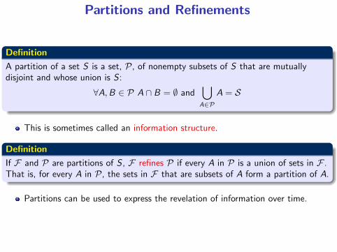
DefinitionA partition of a set S is a set, P, of nonempty subsets of S that are mutuallydisjoint and whose union is S :

∀A,B ∈ P A ∩ B = ∅ and⋃A∈P

A = S

This is sometimes called an information structure.

DefinitionIf F and P are partitions of S , F refines P if every A in P is a union of sets in F .That is, for every A in P, the sets in F that are subsets of A form a partition of A.

Partitions can be used to express the revelation of information over time.

Information Over Time and Dated Events

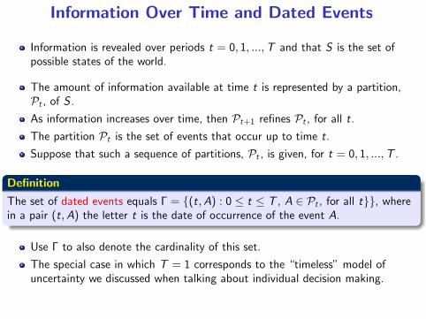
Information is revealed over periods t = 0, 1, ...,T and that S is the set ofpossible states of the world.

The amount of information available at time t is represented by a partition,Pt , of S .As information increases over time, then Pt+1 refines Pt , for all t.The partition Pt is the set of events that occur up to time t.Suppose that such a sequence of partitions, Pt , is given, for t = 0, 1, ...,T .

Definition

The set of dated events equals Γ = {(t,A) : 0 ≤ t ≤ T , A ∈ Pt , for all t}}, wherein a pair (t,A) the letter t is the date of occurrence of the event A.

Use Γ to also denote the cardinality of this set.

The special case in which T = 1 corresponds to the “timeless”model ofuncertainty we discussed when talking about individual decision making.

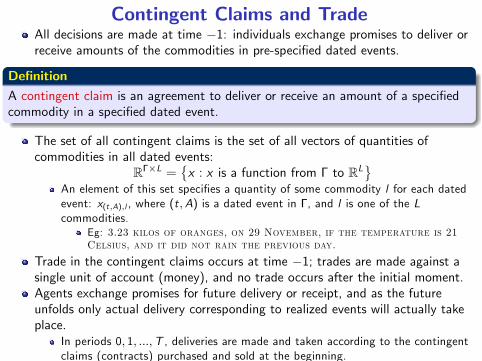
Contingent Claims and TradeAll decisions are made at time −1: individuals exchange promises to deliver orreceive amounts of the commodities in pre-specified dated events.

DefinitionA contingent claim is an agreement to deliver or receive an amount of a specifiedcommodity in a specified dated event.

The set of all contingent claims is the set of all vectors of quantities ofcommodities in all dated events:

RΓ×L ={x : x is a function from Γ to RL

}An element of this set specifies a quantity of some commodity l for each datedevent: x(t,A),l , where (t,A) is a dated event in Γ, and l is one of the Lcommodities.

Eg: 3.23 kilos of oranges, on 29 November, if the temperature is 21Celsius, and it did not rain the previous day.

Trade in the contingent claims occurs at time −1; trades are made against asingle unit of account (money), and no trade occurs after the initial moment.Agents exchange promises for future delivery or receipt, and as the futureunfolds only actual delivery corresponding to realized events will actually takeplace.

In periods 0, 1, ...,T , deliveries are made and taken according to the contingentclaims (contracts) purchased and sold at the beginning.

General Equilibrium Under UncertaintyDefinitions

For each commodity l = 1, .., L, and each dated event in (t,A) ∈ Γ, one unitof state-contingent commodity l (t,A) is a title to receive one unit of good l ifand only if event A at time t occurs.

A state-contingent commodity vector

x ∈ RΓ×L

is a title to receive the commodity vector x(t,A) ∈ RL if and only if dated event(t,A) occurs.

These are binding promises to obtain certain quantities of each of the goods ina given state, after that state is realized:

state-contingent commodities are ‘contracts’.

A state-contingent commodity vector is a random variable: it assigns a vectorin RL to each dated event.

REMARK: All State Contingent Commodities Are TradedWe assume that there is a market for each of these state contingentcommodities.

Preferences Over State Contingent Goods

Expected Utility Preferences Over State Contingent Commodities

Agent i’s consumption set Xi ⊂ RΓ×L+ contains state-contingent commodities.

Agent i’s preferences %i are over Xi .Preferences take into account the passage of time time as well as uncertainty.Typically, later consumption is less “valuable” than earlier consumption, andless likely events are not as “valuable” as more likely events.

These are ex-ante preferences; they describe what i thinks at time −1 aboutwhat she would like to consume in the future.

i makes trade-offs between random variables; one more unit of good l in datedevent (t,A) versus one less unit of good l ′ in dated event (t ′,A′);

Preferences reflect consumers probability distributions across dated events.

The latter are ‘subjective’probabilities.

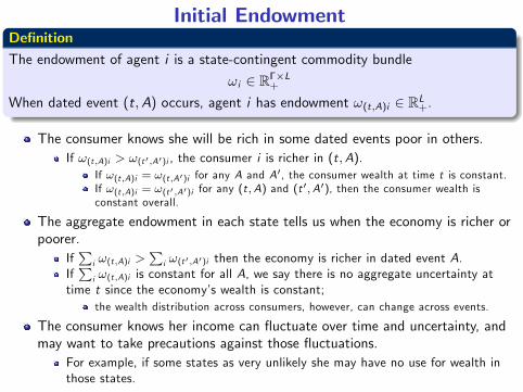
Initial EndowmentDefinitionThe endowment of agent i is a state-contingent commodity bundle

ωi ∈ RΓ×L+

When dated event (t,A) occurs, agent i has endowment ω(t,A)i ∈ RL+.

The consumer knows she will be rich in some dated events poor in others.If ω(t,A)i > ω(t′,A′)i , the consumer i is richer in (t,A).

If ω(t,A)i = ω(t,A′)i for any A and A′, the consumer wealth at time t is constant.If ω(t,A)i = ω(t′,A′)i for any (t ,A) and (t ′,A′), then the consumer wealth isconstant overall.

The aggregate endowment in each state tells us when the economy is richer orpoorer.

If∑

i ω(t,A)i >∑

i ω(t′,A′)i then the economy is richer in dated event A.If∑

i ω(t,A)i is constant for all A, we say there is no aggregate uncertainty attime t since the economy’s wealth is constant;

the wealth distribution across consumers, however, can change across events.

The consumer knows her income can fluctuate over time and uncertainty, andmay want to take precautions against those fluctuations.

For example, if some states as very unlikely she may have no use for wealth inthose states.

Trade Under Uncertainty

Consumers know that their wealth may fluctuate.

This is because consumer i’s initial endowment ω(t,A) changes with the (t,A).

maybe i’s endowment is large in one dated event and small in another; ormaybe i’s endowment of desirable goods is large in some dated events andsmall in others.

Without trade, consumers cannot insure themselves against these income andconsumpion fluctuations.

Trade allows for insurance.

They can sell their initial endowment in some dated events, and use theproceeds to buy consumption in other states; orthey can sell some their initial endowment of particular goods in dated events inwhich they will have a lot of those, and use the proceeds to buy more of othergoods in those states; or a combination of all these things.

Markets for state-contingent commodities make these trades possible.

Production Plans for State Contingent Goods

Like consumers, firms make decisions at time −1 while actual production takesplace from time 0 onward.

They decide what output vector to produce in each dated event.

Production plans are also state-contingent vectors.

Definition

The production possibility set is represented by a set Yj ⊂ RΓ×L for each firm j .

Firms ‘produce’state-contingent commodities.

A y ∈ RΓ×L is a binding promise to buy the corresponding inputs and sell thecorresponding outputs in each dated event.

The firm sells future production and makes a profit that is distributed toconsumers.

Shares in the firms are not state contingent, nor are they traded, but this isjust to keep notation simple.

Markets and Prices in an Arrow-Debreu EconomyIn the Arrow-Debreu model each state-contingent commodity is traded.

Arrow-Debreu MarketsThere are Γ× S markets open at date −1.In these markets, a trade specifies various amounts of goods to be delivered invarious states:

there is a price for each good in each state

pl(t,A) is the price agreed upon now for one unit of good l to be delivered indated event (t ,A).

Agents trade promises to receive, or give, amounts of good l if and when eventA occurs at time t.

In finance lingo, these are “forward”markets where “futures” are traded.

Trades of these ‘contracts’are agreed upon now by all parties involved.Even though decisions are made now, the ‘physical’exchange of goods onlyhappens after uncertainty is resolved.This system of payments and deliveries is well defined only if everyone knowswhich state occurred: symmetric information.

We prevent situations where i says “This is event A” and j says “No, this isevent A′”; if that happens, state-contingent markets may not function properly.

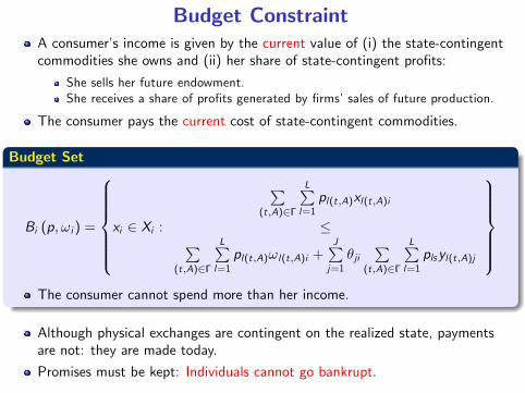
Budget ConstraintA consumer’s income is given by the current value of (i) the state-contingentcommodities she owns and (ii) her share of state-contingent profits:

She sells her future endowment.She receives a share of profits generated by firms’sales of future production.

The consumer pays the current cost of state-contingent commodities.

Budget Set

Bi (p, ωi ) =

xi ∈ Xi :

∑(t,A)∈Γ

L∑l=1pl(t,A)xl(t,A)i

≤∑(t,A)∈Γ

L∑l=1pl(t,A)ωl(t,A)i +

J∑j=1

θji∑

(t,A)∈Γ

L∑l=1plsyl(t,A)j

The consumer cannot spend more than her income.

Although physical exchanges are contingent on the realized state, paymentsare not: they are made today.

Promises must be kept: Individuals cannot go bankrupt.

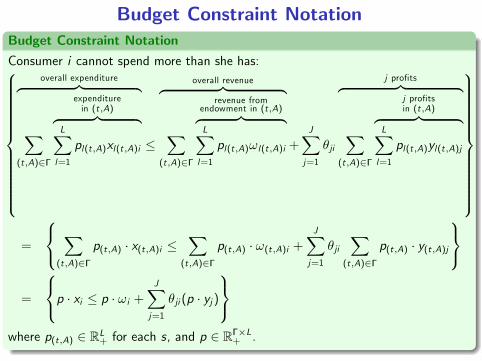
Budget Constraint NotationBudget Constraint NotationConsumer i cannot spend more than she has:

overall expenditure︷ ︸︸ ︷∑

(t,A)∈Γ

expenditurein (t,A)︷ ︸︸ ︷

L∑l=1

pl(t,A)xl(t,A)i ≤

overall revenue︷ ︸︸ ︷∑

(t,A)∈Γ

revenue fromendowment in (t,A)︷ ︸︸ ︷L∑l=1

pl(t,A)ωl(t,A)i +J∑j=1

θji

j profits︷ ︸︸ ︷∑

(t,A)∈Γ

j profitsin (t,A)︷ ︸︸ ︷

L∑l=1

pl(t,A)yl(t,A)j

=

∑(t,A)∈Γ

p(t,A) · x(t,A)i ≤∑

(t,A)∈Γ

p(t,A) · ω(t,A)i +J∑j=1

θji∑

(t,A)∈Γ

p(t,A) · y(t,A)j

=

p · xi ≤ p · ωi +J∑j=1

θji (p · yj )

where p(t,A) ∈ RL+ for each s, and p ∈ RΓ×L

+ .

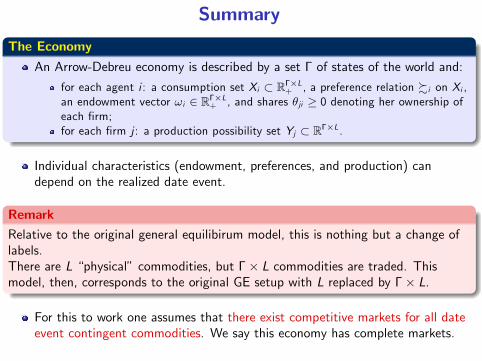
Summary

The EconomyAn Arrow-Debreu economy is described by a set Γ of states of the world and:

for each agent i : a consumption set Xi ⊂ RΓ×L+ , a preference relation %i on Xi ,

an endowment vector ωi ∈ RΓ×L+ , and shares θji ≥ 0 denoting her ownership of

each firm;for each firm j : a production possibility set Yj ⊂ RΓ×L.

Individual characteristics (endowment, preferences, and production) candepend on the realized date event.

RemarkRelative to the original general equilibirum model, this is nothing but a change oflabels.There are L “physical” commodities, but Γ× L commodities are traded. Thismodel, then, corresponds to the original GE setup with L replaced by Γ× L.

For this to work one assumes that there exist competitive markets for all dateevent contingent commodities. We say this economy has complete markets.

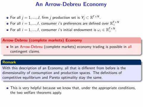
An Arrow-Debreu Economy

For all j = 1, ..., J, firm j production set is Yj ⊂ RΓ×N .

For all i = 1, ..., I , consumer i’s preferences are defined over RΓ×N+

For all i = 1, ..., I , consumer i’s initial endowment is ωi ∈ RΓ×N+ .

Arrow-Debreu (complete markets) Economy

In an Arrow-Debreu (complete markets) economy trading is possible in allcontingent claims.

RemarkWith this description of an Economy, all that is different from before is thedimensionality of consumption and production spaces. The definitions ofcompetitive equilibrium and Pareto optimality stay the same.

This is very helpful because we know that, under the appropriate conditions,the two welfare theorems apply.

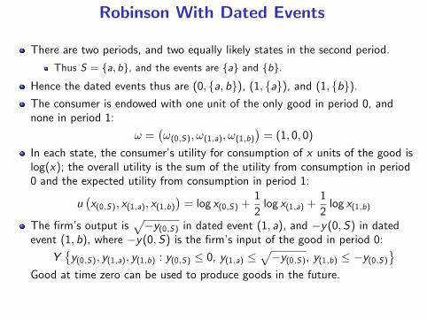
Robinson With Dated Events

There are two periods, and two equally likely states in the second period.

Thus S = {a, b}, and the events are {a} and {b}.

Hence the dated events thus are (0, {a, b}), (1, {a}), and (1, {b}).The consumer is endowed with one unit of the only good in period 0, andnone in period 1:

ω =(ω(0,S), ω(1,a), ω(1,b)

)= (1, 0, 0)

In each state, the consumer’s utility for consumption of x units of the good islog(x); the overall utility is the sum of the utility from consumption in period0 and the expected utility from consumption in period 1:

u(x(0,S), x(1,a), x(1,b)

)= log x(0,S) +

12log x(1,a) +

12log x(1,b)

The firm’s output is√−y(0,S) in dated event (1, a), and −y(0,S) in dated

event (1, b), where −y(0, S) is the firm’s input of the good in period 0:

Y{y(0,S), y(1,a), y(1,b) : y(0,S) ≤ 0, y(1,a) ≤

√−y(0,S), y(1,b) ≤ −y(0,S)

}Good at time zero can be used to produce goods in the future.

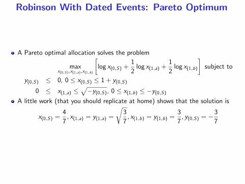
Robinson With Dated Events: Pareto Optimum

A Pareto optimal allocation solves the problem

maxx(0,S),x(1,a),x(1,b)

[log x(0,S) +

12log x(1,a) +

12log x(1,b)

]subject to

y(0,S) ≤ 0, 0 ≤ x(0,S) ≤ 1+ y(0,S)

0 ≤ x(1,a) ≤√−y(0,S), 0 ≤ x(1,b) ≤ −y(0,S)

A little work (that you should replicate at home) shows that the solution is

x(0,S) =47, x(1,a) = y(1,a) =

√37, x(1,b) = y(1,b) =

37, y(0,S) = −3

7

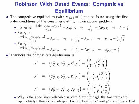
Robinson With Dated Events: CompetitiveEquilibrium

The competitive equilibrium (with p(0,S) = 1) can be found using the firstorder conditions of the consumer’s utility maximization problem.

For x(0,S):∂u(x(0,S),x(1,a),x(1,b))

∂x(0,S)= λp(0,S) ⇒ 1

x(0,S)= λp(0,S) ⇒ λ = 7

4

For x(1,a):∂u(x(0,S),x(1,a),x(1,b))

∂x(1,a)= λp(1,a) ⇒ 1

21

x(1,a)= λp(1,a) ⇒ p(1,a) = 2

7

√73

For x(1,b):∂u(x(0,S),x(1,a),x(1,b))

∂x(1,b)= λp(1,b) ⇒ 1

21

x(1,b)= λp(1,b) ⇒ p(1,b) = 2

3

Therefore the competitive equilibirum is

x∗ =(x∗(0,S), x

∗(1,a), x

∗(1,b)

)=

(47,

√37,37

)

y∗ =(y∗(0,S), y

∗(1,a), y

∗(1,b)

)=

(−37,

√37,37

)

p∗ =(p∗(0,S), p

∗(1,a), p

∗(1,b)

)=

(1,27

√73,23

)Why is the good more valueable in state b even though the two states areequilly likely? How do we interpret the numbers for x∗ and y∗? are they actualgoods being consumed?

General Equilibrium Under Uncertainty Alone

Suppose there is no time and there are S states.

The set of all vectors of contingent claims is RS×L

One can think of each commodity bundle as an S-dimensional random variable(a random vector).

If there is only one commodity, L = 1, one typically thinks of it as money.

Rather than labeling dated events as (0, {s}) for each s ∈ S we may as welldrop the 0 and just label each event by the realized state s.

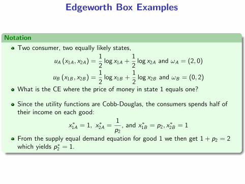
Edgeworth Box Examples

NotationTwo consumer, two equally likely states,

uA (x1A, x2A) =12log x1A +

12log x2A and ωA = (2, 0)

uB (x1B , x2B ) =12log x1B +

12log x2B and ωB = (0, 2)

What is the CE where the price of money in state 1 equals one?

Since the utility functions are Cobb-Douglas, the consumers spends half oftheir income on each good:

x∗1A = 1, x∗2A =1p2, and x∗1B = p2, x∗2B = 1

From the supply equal demand equation for good 1 we then get 1+ p2 = 2which yields p∗2 = 1.

Edgeworth Box Examples

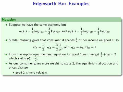
NotationSuppose we have the same economy but

uA (·) =14log x1A +

34log x2A and uB (·) =

12log x1B +

12log x2B

Similar reasning gives that consumer A spends 14 of her income on good 1, so

x∗1A =12, x∗2A =

321p2, and x∗1B = p2, x∗2B = 1

From the supply equal demand equation for good 1 we then get 12 + p2 = 2which yields p∗2 = 3

2 .

As one consumer gives more weight to state 2, the equilibrium allocation andprices change.

good 2 is more valuable.

Edgeworth Box Examples

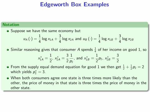
NotationSuppose we have the same economy but

uA (·) =14log x1A +

34log x2A and uB (·) =

14log x1B +

34log x2B

Similar reasoning gives that consumer A spends 14 of her income on good 1, so

x∗1A =12, x∗2A =

321p2, and x∗1B =

12p2, x∗2B =

32

From the supply equal demand equation for good 1 we then get 12 + 12p2 = 2

which yields p∗2 = 3.

When both consumers agree one state is three times more likely than theother, the price of money in that state is three times the price of money in theother state.

Next Week

Focus on the model in which there is no time.

Introduce financial markets.