article functional model of residential consumption
TRANSCRIPT

Elsevier 2021, 05, x; doi: FOR PEER REVIEW www.elsevier.com/locate/enbuild
Article
Functional Model of Residential Consumption
Elasticity under Dynamic Tariffs
Kamalanathan Ganesan 1,2*, João Tomé Saraiva 1,2 and Ricardo J. Bessa 2
1 Faculty of Engineering, University of Porto (FEUP), 4200-465 Porto, Portugal; [email protected] 2 INESC Technology and Science (INESC TEC), 4200-465 Porto, Portugal; [email protected],
* Correspondence: [email protected]
Abstract: One of the major barriers for the retailers is to understand the consumption elasticity they
can expect from their contracted demand response (DR) clients. The current trend of DR products
provided by retailers are not consumer-specific, which poses additional barriers for the active
engagement of consumers in these programs. The elasticity of consumers’ demand behavior varies
from individual to individual. The utility will benefit from knowing more accurately how changes
in its prices will modify the consumption pattern of its clients. This work proposes a functional
model for the consumption elasticity of the DR contracted consumers. The model aims to determine
the load adjustment the DR consumers can provide to the retailers or utilities for different price
levels. The proposed model uses a Bayesian probabilistic approach to identify the actual load
adjustment an individual contracted client can provide for different price levels it can experience.
The developed framework provides the retailers or utilities with a tool to obtain crucial information
on how an individual consumer will respond to different price levels. This approach is able to
quantify the likelihood with which the consumer reacts to a DR signal and identify the actual load
adjustment an individual contracted DR client provides for different price levels they can
experience. This information can be used to maximize the control and reliability of the services the
retailer or utility can offer to the System Operators.
Keywords: Bayesian probabilistic model, consumption elasticity; causal inference; data-driven;
demand response; residential consumers
1. Introduction
1.1 Context and Motivation
The current residential demand response (DR) programs’ engagement is far from its achievable
potential because of a lack of addressing the barriers that largely vary between contracted individual
consumers [1]. The aggregators and retailers must incorporate possible directions to modify
consumption patterns along with their DR signals to clients, who are allowed to take free actions in
reaction to the signals (e.g., economic, environmental) they receive. This will lead to confident
participation of the consumers without their current concerns of energy security and privacy. This
approach, on the other hand, will cause some concerns for the retailers regarding the reliability of the
bids they make in the wholesale market.
Engaging the residential consumers and providing the best tariffs for their randomized
behaviors is one of the major barriers identified in DR studies [2]. One of the major assumptions made
by competitive electricity markets around the world which envision implementing (or currently work
with) DR programs is that they assume the end-users (specifically residential consumers) will adopt
the best decision available to them [3]. This generally results to assuming they react to DR prices as
expected, accept direct load control and home automation, and participate in planned and predicted
household activities that facilitate response to the price signals sent to them. But this is not the case
from a behavioral economics perspective as consumers have limited knowledge of the benefits from

PRE-PRINT FOR PEER REVIEW 2 of 28
actively participating in these programs. The actors’ behaviors are more inclined to changes, which
will not always be predictably proportional to prices [2, 4].
The most common residential DR programs involve customers shifting load manually in
response to price signals. However, research has also looked at home automation systems that
monitor and control the consumption of typical household appliances, ranging from AC’s, washing
machines, dishwashers to electric water heaters. From a general perspective, even with advanced
metering technologies and reasonable experience with DR programs, the adoption of these strategies
at the residential level is still limited. This could be due to the reason that DR pricing schemes could
eventually lead to rebound effects, such cases when day-ahead hourly prices are applied new peak
demand periods may arise [5]. However, it is reported that a considerable amount of residential load
will be available for shifting for the utilities to balance the system. Nevertheless, the investments
made by households on smart devices will not prove to be economic from their perspective.
DR resources cannot yet completely compete on an equal level with traditional (generation)
resources. In addition, for household consumers, it is not easy to offer services on an individual basis.
Therefore, DR service providers could for instance aggregate demand response of multiple similar
end-consumers and sell it to the market as an aggregated bundle consumer [6-8]. In this case, service
providers can make a pool of combined loads that they sell as a single resource and as such help
individual consumers to value their flexibility potential.
1.2 Related Work and Contributions
One main challenge while studying a DR program is the ability of the model to distinguish a
normal consumption from a DR instigated consumption. Lopes et al. [9] and Navigant [10] used a
non-regression technique which compares the mean hourly consumption on event days to that of
non-event days for the same household. George et al. [11] and Ericson [12] used a multiple regression
technique where the regression coefficients are the estimates of the program effects and the events
are the independent variables. Herter et al. [13] compares CPP households’ average peak-time
weekday loads to their normal-time average weekday loads for the same temperature (to avoid
temperature bias) to identify the change in demand. Zhou et al. [14] used machine learning
techniques to predict residential electricity consumption with non-parametric hypothesis to identify
the reduction in household consumption during DR events. However, all these studies fail to quantify
the likelihood with which the consumers alter their consumption behavior during DR events.
In [15], the author’s idea was also to model an adaptive learning agent with reinforcement
learning. A profit-seeking intelligent retailer makes repeated interactions with its clients to adapt its
DR strategy based on the price elasticity of demand. The consumers have assumed/allotted self-
elasticity values which determine their demand reduction potential during DR events. The drawback
with using reinforcement learning in understanding consumer behavior is that one cannot establish
a causal relationship linking the current state of the environment to the previous action. This could
lead to undesirable action selection policy for the next state, and thus deviate from the actual behavior
of a consumer. This is one of the reasons why both these studies have resorted to using clustered
consumers’ load and elasticity profile instead of individual consumers.
In a theoretical study done by H. C. Gils [16], substantial potential for demand response was
found amongst residential consumers. According to some sources, “It is now clear to policymakers that
Europe will not be able to achieve its energy policy goals in a secure and cost-efficient manner unless the energy
system becomes more flexible. DR and consumer empowerment are understood as integral parts of the Energy
Union and the Clean Energy Package for all Europeans because they help to reach a competitive, secure, and
sustainable economy” [17]. Europe is now expanding on this model by giving individuals and
communities the right to produce, store and sell energy. The revised Renewable Energy Directive
RED II [18] and the Internal Electricity Market (IEM) Directive [19] introduced the concepts of
Renewable Energy Community (REC) and of Citizen Energy Community (CEC), as part of the final
Clean Energy Package. As such, Europe is giving consumers a way to organize themselves
individually, or as a community, to ensure a more open energy-sector while empowering consumers
in the context of the energy markets.
PRE-PRINT FOR PEER REVIEW 3 of 28
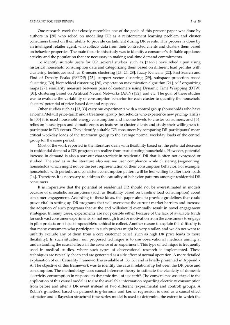
One research work that closely resembles one of the goals of this present paper was done by
authors in [20] who relied on modelling DR as a reinforcement learning problem and cluster
consumers based on their ability to provide curtailment during DR events. This process is done by
an intelligent retailer agent, who collects data from their contracted clients and clusters them based
on behavior properties. The main focus in this study was to identify a consumer’s shiftable appliance
activity and the population that are necessary in making real-time demand commitments.
To identify suitable users for DR, several studies, such as [21-27] have relied upon using
historical household consumption data and categorizing them based on different load profiles with
clustering techniques such as K-means clustering [23, 24, 28], fuzzy K-means [22], Fast Search and
Find of Density Peaks (FSFDP) [25], support vector clustering [29], subspace projection based
clustering [30], hierarchical clustering [26], expectation maximization algorithm [21], self-organizing
maps [27], similarity measure between pairs of customers using Dynamic Time Wrapping (DTW)
[31], clustering based on Artificial Neural Networks (ANN) [32], and etc. The goal of these studies
was to evaluate the variability of consumption behavior for each cluster to quantify the household
clusters’ potential of price-based demand response.
Other studies such as [13, 33] carry out experiments with a control group (households who have
a normal/default price-tariff) and a treatment group (households who experience new pricing-tariffs).
In [33] it is used household energy consumption and income levels to cluster consumers, and [34]
relies on house types and climatic zones as features to cluster clients and study their willingness to
participate in DR events. They identify suitable DR consumers by comparing DR participants’ mean
critical weekday loads of the treatment group to the average normal weekday loads of the control
group for the same period.
Most of the work reported in the literature deals with flexibility based on the potential decrease
in residential demand a DR program can realize from participating households. However, potential
increase in demand is also a sort-out characteristic in residential DR that is often not expressed or
studied. The studies in the literature also assume user compliance while clustering (segmenting)
households which might not be the best representation of their consumption behavior. For example,
households with periodic and consistent consumption pattern will be less willing to alter their loads
[14]. Therefore, it is necessary to address the causality of behavior patterns amongst residential DR
consumers.
It is imperative that the potential of residential DR should not be overestimated in models
because of unrealistic assumptions (such as flexibility based on baseline load consumption) about
consumer engagement. According to these ideas, this paper aims to provide guidelines that could
prove vital in setting up DR programs that will overcome the current market barriers and increase
the adoption of such programs that at the end will/should eventually result in novel engagement
strategies. In many cases, experiments are not possible either because of the lack of available funds
for such vast consumer experiments, or not enough trust or motivation from the consumers to engage
in pilot projects or it is just impossible/unethical to collect. Another reason to explain this difficulty is
that many consumers who participate in such projects might be very similar, and we do not want to
unfairly exclude any of them from a core customer belief (such as high DR price leads to more
flexibility). In such situation, our proposed technique is to use observational methods aiming at
understanding the causal effects in the absence of an experiment. This type of technique is frequently
used in medical studies, where such types of observational research is implemented. These
techniques are typically cheap and are generated as a side effect of normal operation. A more detailed
explanation of our Causality Framework is available at [35, 36] and is briefly presented in Appendix
A. The objective of this framework was to identify the causal relationship between the DR price and
consumption. The methodology uses causal inference theory to estimate the elasticity of domestic
electricity consumption in response to dynamic time-of-use tariff. The convenience associated to the
application of this causal model is to use the available information regarding electricity consumption
from before and after a DR event instead of two different (experimental and control) groups. A
Robin’s g-method based on parametric g-formula and kernel regression is used as a causal effect
estimator and a Bayesian structural time-series model is used to determine the extent to which the

PRE-PRINT FOR PEER REVIEW 4 of 28
price changes impact on the consumer’s consumption. This gives us a likelihood probability of the
price having a causal effect on the consumption. The model provides the potential to help the utilities
or retailers to estimate the available elasticity from each of their contracted consumers in the scope of
DR programs for each of the price signals they have experienced during the DR program.
Thus, in this paper, using the elasticity values we have from the causality inference framework,
we build a functional model for the consumer’s elasticity. This functional model will output a curve
relating the load adjustment (elasticity provided) to the prices experienced by the consumers under
different scenarios (outside temperature, time of day, day, month, etc.). This will eventually provide
us with an elasticity behavior model for each consumer. The upside of using this technique is that it
incorporates useful information, and the considered parameters will relate to the absolute effects that
can occur in electricity consumption changes.
The main original contributions from this paper can be classified into two folds. The first one is
a consumer probability score model based on the Dirichlet-multinomial distribution and Bayesian
inference. The model is built based on the observed elasticities and their weights from the causality
framework. With model parameters such as the beta-distribution and pseudo-counts relating to each
consumer, a Bayesian inference is used to identify the distribution of a consumer’s acceptance
probability (when a set of consumers are grouped together for an event). The second original
contribution is an approach using Bayesian probabilistic programming to use the elasticity of the
consumer’s demand response to the offers they receive from the market/retailers and use them to
estimate probabilities of elasticity values for unseen (unexperienced) tariffs. This will give a clear
picture to the retailers in terms of the impact such offers make on a specific client, i.e. if the tariff is
lower or increases twice its rate for a given period, how would that client react to such variations. It
gives an insight into what price levels each consumer was more susceptible to and what was the
untapped potential from underperforming consumers.
1.3 Structure of the Paper
After this introductory section, Section 2 describes the residential consumption data from
London electricity pricing trial (available in open access) and general methodology, Section 3
describes the developed Bayesian probabilistic methodology for estimating consumers probability
score for experienced DR prices and Section 4 describes the estimation of consumption elasticity to
unexperienced DR prices, and Section 5 enumerates the most relevant conclusions. Finally, Appendix
A provides a brief description of the adopted Causality model.
2. Data Collection and Methodology
2.1 Dataset Description
The Low Carbon London (LCL) project was UK’s first residential sector, time-of-use electricity
pricing trial. UK Power Networks and EDF Energy jointly performed this project. The trial involved
5667 households organized in two groups, one the target group and the other the control group. The
group that was influenced by dynamic Time-Of-Use tariffs (dToU group) consisted of 1122
households and the control group, which remained with existing non-dynamic Time-Of-Use tariff
(non-ToU), consisted of 4545 consumers [37]. The electricity consumption was measured every 30
mins from 2012 (July–December) till 2013 (full year) for the dynamic Time-Of-Use (dToU) group from
which we selected 81 clients. The dataset also contained tariff information, which comprised of three
rates for the year 2013: Default is 0.1176 £/kWh; high is 0.6720 £/kWh; low is 0.0390 £/kWh. These
rates were applicable to the dToU group only for the year 2013, whereas a flat tariff of 0.1176 £/kWh
was maintained for the year 2012. Customers were informed of upcoming price changes one day
ahead of delivery via notifications that appeared on their smart-meter linked in-home-display and
also, if requested, via short message service (SMS) messages to their mobile phones. The price events
were based on system balancing (lasted between 3 h to 12 h) and distribution network constraint
management signals (which lasted for nearly 24 h) received by the retailers.

PRE-PRINT FOR PEER REVIEW 5 of 28
We use 81 dToU clients who have the best-recorded values and after data cleaning provide the
best featured collection of consumers. The LCL dataset included an appliance survey dataset which
collected information such as appliance ownership, physical parameters of the premises (either,
house, apartment or mobile house) and basic details of its occupants such as energy decision maker,
household size and age). In our analysis, all 81 clients were considered from the “house” category,
and with household size “2 and higher” to have a consistent result. Other demographic information
was collected in their survey but was not publicly available for using in our analysis. Since weather
related information was not provided with this dataset, daily as well as half-hourly weather data for
the years 2012 and 2013 were collected from an online source [38]. The new dataset was designed to
include the following features for each client:
a) average power (kW) per 30 min interval;
b) hour of consumption;
c) price associated with the consumption period;
d) atmospheric temperature, humidity, pressure, visibility, wind direction, wind speed and
weather conditions (example. Cloudy, clear, rainy fair, etc.);
e) current time of an event, minute, month, day of the week, week of the year, weekday
number;
Building electricity consumption does have a direct causal relationship with the building
occupancy rate. Specific loads such as, plug-loads have a stronger correlation with the occupancy
rates as shown by Kim et al. [39]. Their study estimates about 10%-40% of energy can be saved by
factoring occupancy rates into building energy consumption. As our dataset, does not include the
occupancy rate, we rely on differentiating the “daily routine” and “occupancy lifestyle” by the day
of the week feature in our Causality Inference model, that estimates our elasticities used in the
Elasticity Behavior model.
2.2 Methodology - Bayesian Probabilistic Programing Framework
2.2.1 General Modelling Aspects
The adopted approach to tackle this problem adopts a data-driven Bayesian inference with
probabilistic models. We need to include uncertainty in our estimate considering the data we have
collected about each consumer. Second, we also must incorporate prior beliefs about the situation
into this estimate. If we can assume the temperature variations during days & seasons, occupancy
rate during weekday & weekends, probability of acting towards DR signal, etc., then surely this
should play some role in our estimate. Thus, to allow our model to express such uncertainty and
incorporate prior information into the estimates, we rely on Bayesian inference techniques. This
section explores the problem of estimating probabilities from our data in a Bayesian Framework,
along the way learning about probability distributions, Bayesian Inference and probabilistic
programming.
Bayesian Inference is based in the fact that the truth is somewhere in-between the prior
knowledge of the scenario under consideration, and the observed data. Building a constructive
relationship between the prior belief and the observed data can result in the posterior belief of a
model. This is expressed using the Bayes Formula given by (1).
𝑝(𝜃|𝑋) = 𝑝(𝑋|𝜃) . 𝑝(𝜃)
𝑝(𝑋) (1)
𝑝(𝑋) = ∑ 𝑝(𝑋|𝜃) . 𝑝(𝜃)
𝜃
(2)
𝑝(𝜃|𝑋) = 𝑝(𝑋|𝜃) . 𝑝(𝜃) (3)
In (1), X is the data variable whose value we observe as x and estimate p(θ), a parameter of an
unknown variable Y. We see that the Bayes Theorem expresses the posterior density p(θ|X), in terms

PRE-PRINT FOR PEER REVIEW 6 of 28
of likelihood p(X|θ) and prior p(θ), along with the marginal likelihood p(X) which is usually the
normalization term given by Equation (2). We then can express the posterior probability distribution
function p(θ│X) as described by Equation (3).
The Markov Chain Monte Carlo (MCMC) method can be used for estimating the parameters (θ)
of a random model (such as Equation (1)), by running the model for a large number of iterations
within a reasonable amount of time. The model’s likelihood function and prior distribution will be
used to draw the trajectory (such as trees) through the space for all possible values of θ. So, in a way,
one should make sure the prior and the likelihood relationship to be as accurate as possible to
estimate the best estimate fit for θ based on the observations. The posterior density given by equation
(2) is used to guide the Markov chain S = (θ1,..θn) through the parameter space for all the possible
value settings of θ. After drawing many samples from the defined model, we converge to an
approximately desired posterior along with their uncertainties. Probabilistic Programing (PP) is a
programming technique to unify probability models and inferences for these models to help make
better decisions when faced with uncertain situations. The idea behind PP is to bring the inference
algorithms and theory from statistics combined with formal semantics, compilers, and other tools to
build efficient inference evaluators for models and applications from Machine Learning.
In other words, probabilistic programming is a tool for Bayesian statistical modeling.
Probabilistic thinking is an incredibly valuable tool for decision making. From economists to poker
players, people that can think in terms of probabilities tend to make better decisions when faced with
uncertain situations. Probabilistic programming (PP) allows flexible specification of Bayesian
statistical models in code. In our work, we use a Python framework called PYMC which performs the
probabilistic programming using Theano, that allows for automatic Bayesian inference on user-
defined probabilistic models. Model assumptions are recorded with prior distributions over the
variables that influence the model. At the execution level, the model will launch the inference
procedure to automatically compute the posterior distribution of the parameters of the model based
on observed data. This is done in a way that the inference adjusts the prior distribution using the
observed data as a base, to give a more precise mode. Recent advances in Markov Chain Monte Carlo
(MCMC) sampling allow inference on increasingly complex models. PYMC features next-generation
Markov Chain Monte Carlo (MCMC) sampling algorithms such as the No-U-Turn Sampler (NUTS,
[40]), a self-tuning variant of Hamiltonian Monte Carlo (HMC, [41]). HMC and NUTS take advantage
of gradient information from the likelihood to achieve much faster convergence than traditional
sampling methods, especially for larger models. NUTS also has several self-tuning strategies for
adaptively setting the tunable parameters of Hamiltonian Monte Carlo.
3. Consumer Response Probability Score
The first main original contribution from this paper is based on a methodology using the
Dirichlet-multinomial distribution [42]. In Bayesian statistics, the parameter vector for a multinomial
function is drawn from a Dirichlet Distribution, which forms the prior distribution for the parameter.
In Bayesian probability theory, conjugate distribution or conjugate pair means a pair of a sampling
distribution and a prior distribution for which the resulting posterior distribution belongs into the
same parametric family of distributions than the prior distribution, and the prior is called a conjugate
prior for this sampling distribution. Even with increasingly better computational tools, such as
MCMC, models based on conjugate distributions are advantageous. One such conjugate distribution
is the Beta-Binomial distribution which is based on binary choices, and a generalization of Beta
distribution is called the Dirichlet-Distribution which is based on multiple choices. It corresponds to
a family of discrete multivariate probability distributions on a finite support of non-negative integers.
The Dirichlet distribution models the probabilities of multiple mutually exclusive choices,
parameterized by “alpha” (which is referred to as the concentration parameter) and represents the
weights for each choice. In the literature, we encounter the Dirichlet distribution often in the context
of topic modeling in natural language processing, where it is commonly used as part of a Latent
Dirichlet Allocation (or LDA) model. However, for our purposes, we look at the Dirichlet-
PRE-PRINT FOR PEER REVIEW 7 of 28
Multinomial in the context of acceptance probability for the responses to the DR price signals received
by the consumers.
3.1 Methodology
To identify the probability of accepting/acting to change consumption for a given price signal,
we use Bayesian methods to look for the posterior probability. Thus, we construct a model for this
situation with the series of observed elasticities (as collected from the Causality Framework
developed in [36]) and their ranking (model defined weights). For our model, we have a case where
unlike in binomial distributions (just having 2 possible outcomes) we have many outcomes which
means that we are dealing with a multinomial distribution. Our multinomial distribution is
characterized by the following parameters;
n = sum of the weights associated with elasticity
theta (𝜃) = Dirichlet distribution of alpha (vector of probabilities for each of the
outcomes)
alpha (𝛼) = concentration parameter
p = event probability for each consumer (parameters of multinomial)
c = observed elasticity weights data
h = Time period (hour) of the observed data
i = Either “Price” or “Consumer” depending on model chosen
k = number of outcomes (either number of prices or consumers) depending
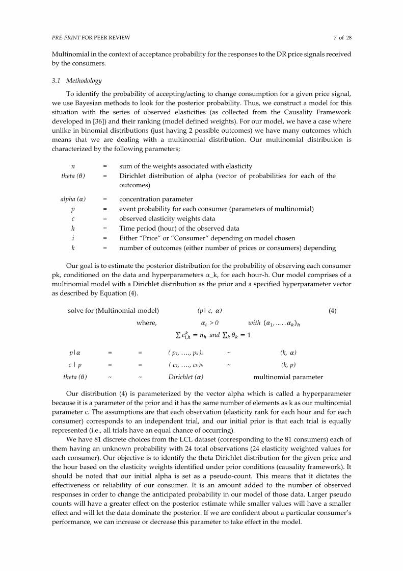
on model chosen Our goal is to estimate the posterior distribution for the probability of observing each consumer
pk, conditioned on the data and hyperparameters α_k, for each hour-h. Our model comprises of a
multinomial model with a Dirichlet distribution as the prior and a specified hyperparameter vector
as described by Equation (4).
solve for (Multinomial-model) (p| c, 𝛼) (4)
where, 𝛼𝑖 > 0 with (𝛼1, … . . 𝛼𝑘)ℎ
∑ 𝑐𝑖,ℎ𝑘 = 𝑛ℎ and ∑ 𝜃𝑘𝑘 = 1
p|𝛼 = = ( p1, …., pk )h ~ (k, 𝛼)
c | p = = ( c1, …., ck )h ~ (k, p)
theta (𝜃) ~ ~ Dirichlet (𝛼) multinomial parameter
Our distribution (4) is parameterized by the vector alpha which is called a hyperparameter
because it is a parameter of the prior and it has the same number of elements as k as our multinomial
parameter c. The assumptions are that each observation (elasticity rank for each hour and for each
consumer) corresponds to an independent trial, and our initial prior is that each trial is equally
represented (i.e., all trials have an equal chance of occurring).
We have 81 discrete choices from the LCL dataset (corresponding to the 81 consumers) each of
them having an unknown probability with 24 total observations (24 elasticity weighted values for
each consumer). Our objective is to identify the theta Dirichlet distribution for the given price and
the hour based on the elasticity weights identified under prior conditions (causality framework). It
should be noted that our initial alpha is set as a pseudo-count. This means that it dictates the
effectiveness or reliability of our consumer. It is an amount added to the number of observed
responses in order to change the anticipated probability in our model of those data. Larger pseudo
counts will have a greater effect on the posterior estimate while smaller values will have a smaller
effect and will let the data dominate the posterior. If we are confident about a particular consumer’s
performance, we can increase or decrease this parameter to take effect in the model.

PRE-PRINT FOR PEER REVIEW 8 of 28
We set up a model to estimate the posterior probability for theta (i.e., the probability of responses
for each price for each hour) for different consumers. We will use the Dirichlet distribution variable
from PYMC model for this purpose along with our observed variable (consumer elasticity ranking
and unobserved (theta) variables. For the prior on theta, we will assume a non-informative uniform
distribution, by initializing the Dirichlet prior with a series of 1s for the parameter alpha, one for each
of the k possible outcomes. This shows that for every hour, the possibility of accepting a price is
always available as our model is reduced to a 24 h scale for the elastic behavior. The expected value
of a multinomial for each hour with Dirichlet priors can be expressed as given by (5).
𝐸[𝑝 | 𝑐ℎ , 𝛼] = 𝑐𝑖 + 𝛼𝑖
𝑛 + ∑ 𝛼𝑘𝑘
(5)
And the Dirichlet probability density function is expressed as (5.6).
𝑝(𝜃1, … . . 𝜃𝑘 | 𝛼1, … . . 𝛼𝑘) = 1
𝐵(𝛼)∏ 𝜃𝑖
𝛼𝑖−1
𝑘
𝑖=1
(6)
In this expression, 𝐵(𝛼) is the multinomial beta function given by (5.7) which normalizes the
distribution (alpha) making sure that the integral equals 1.
𝐵(𝛼) = ∏ Γ(𝛼𝑖)
𝑘𝑖=1
Γ(∑ 𝛼𝑖𝑘𝑖=1 )
(7)
The posterior distribution given by Equation (8a) is solved using Bayesian inference, where we
build the model and then use it to sample (to identify discrete outcomes) from the posterior to
approximate the posterior with No-U-Turn Sampler method in PyMC3. We calculate the posterior
probability of “c” by integrating out theta (𝜃) as indicated from (8a) to (8d).
𝑃(𝑐|𝛼) = ∫ 𝑃(𝑐, 𝜃|𝛼) 𝑑𝜃 = ∫ 𝑃(𝑐|𝜃) 𝑃(𝜃|𝛼) 𝑑𝜃 (8a)
= ∫ (∏ 𝜃𝑖𝑁𝑖
𝑘
𝑖=1
) (1
𝐵(𝛼)∏ 𝜃𝑖
𝛼𝑖−1
𝑘
𝑖=1
) 𝑑𝜃 (8b)
= 1
𝐵(𝛼)∫ ∏ 𝜃𝑖
𝑁𝑖+ 𝛼𝑖−1
𝑘
𝑖=1
𝑑𝜃 (8c)
= 𝐵(𝑁 + 𝛼)
𝐵(𝛼)
(8d)
The result is not just one number but rather a range of samples that lets us quantify our
uncertainty. Our model draws 5000 samples from the posterior in parallel computing (5000 * 4 for a
4 core machine). We adjust the model to use the 1st 1000 samples as tuning samples, and the
inferences are made only after the 1st 1000 samples.
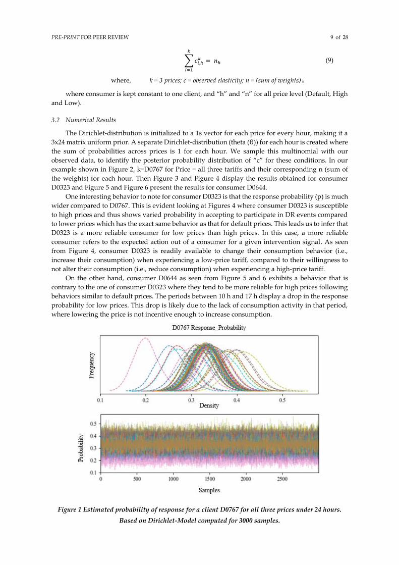
This results in trace samples as shown in Figure 1, which we use to estimate the posterior
probability distribution. The estimate p is the kernel density estimate for the sampled parameters
(PDF of the event probabilities) along with uncertainty. The point estimate of p is the mean of the
posterior trace samples and the Bayesian equivalent confidence interval (called credible interval) are
the 95% and 5% highest probability density. The uncertainty in our posterior reduces with a greater
number of observations. We have the different elasticity profiles for each consumer over different
hours for different prices.
In Figure 1 and Figure 2, the estimate ‘p’ is represented as “Response Probability”. The plot in
Figure 1 shows the p for client D0767 data including all three prices for all 24 hours and Figure 2
shows the mean values of the responses for each price signified by distinct colors and their relative
probability of response for each hour. This is represented as:
PRE-PRINT FOR PEER REVIEW 9 of 28
∑ 𝑐𝑖,ℎ𝑘
𝑘
𝑖=1
= 𝑛ℎ (9)
where, k = 3 prices; c = observed elasticity; n = (sum of weights) h
where consumer is kept constant to one client, and “h” and “n” for all price level (Default, High
and Low).
3.2 Numerical Results
The Dirichlet-distribution is initialized to a 1s vector for each price for every hour, making it a
3x24 matrix uniform prior. A separate Dirichlet-distribution (theta (θ)) for each hour is created where
the sum of probabilities across prices is 1 for each hour. We sample this multinomial with our
observed data, to identify the posterior probability distribution of “c” for these conditions. In our
example shown in Figure 2, k=D0767 for Price = all three tariffs and their corresponding n (sum of
the weights) for each hour. Then Figure 3 and Figure 4 display the results obtained for consumer
D0323 and Figure 5 and Figure 6 present the results for consumer D0644.
One interesting behavior to note for consumer D0323 is that the response probability (p) is much
wider compared to D0767. This is evident looking at Figures 4 where consumer D0323 is susceptible
to high prices and thus shows varied probability in accepting to participate in DR events compared
to lower prices which has the exact same behavior as that for default prices. This leads us to infer that
D0323 is a more reliable consumer for low prices than high prices. In this case, a more reliable
consumer refers to the expected action out of a consumer for a given intervention signal. As seen
from Figure 4, consumer D0323 is readily available to change their consumption behavior (i.e.,
increase their consumption) when experiencing a low-price tariff, compared to their willingness to
not alter their consumption (i.e., reduce consumption) when experiencing a high-price tariff.
On the other hand, consumer D0644 as seen from Figure 5 and 6 exhibits a behavior that is
contrary to the one of consumer D0323 where they tend to be more reliable for high prices following
behaviors similar to default prices. The periods between 10 h and 17 h display a drop in the response
probability for low prices. This drop is likely due to the lack of consumption activity in that period,
where lowering the price is not incentive enough to increase consumption.
Figure 1 Estimated probability of response for a client D0767 for all three prices under 24 hours.
Based on Dirichlet-Model computed for 3000 samples.

PRE-PRINT FOR PEER REVIEW 10 of 28
Figure 2 Consumer D0767’s estimated probability of response to all three prices for each hour from
the Dirichlet-Model
Figure 3 Estimated probability of response for a client D0323 for all three prices under 24 hours.
Based on Dirichlet-Model computed for 3000 samples.

PRE-PRINT FOR PEER REVIEW 11 of 28
Figure 4 Consumer D0323’s estimated probability of response to all three prices for each hour from
the Dirichlet-Model
Figure 5 Estimated probability of response for a client D0644 for all three prices under 24 hours.
Based on Dirichlet-Model computed for 3000 samples.
Figure 6 Consumer D0644’s estimated probability of response to all three prices for each hour from
the Dirichlet-Model

PRE-PRINT FOR PEER REVIEW 12 of 28
Comparing the estimated response probability plots for the three clients shown above, it is
evident that some clients are more susceptible to price changes and show elasticity based on the prices
they experience. This is seen in client D0767 and the price effect is pronounced for client D0323. On
the other hand, client D0644 seems not to be very price-sensitive, but it still shows probabilities of
higher elasticity for different hours. This is clearly seen in the probability density plot of Figure 5 and
Figure 6. It is also imperative for us to identify the difference in response probability for a pool of
consumers. This characterizes how the consumers would react when they are pooled into a selected
group for a given price. Thus, our data fed into the Dirichlet-model is modified to replicate a selected
group of consumers for a single DR price they have experienced. Figure 7 depicts the probability of
response for 5 clients grouped under the Low DR price. This is represented as:
∑ 𝑐𝑖,ℎ𝑘
𝑘
𝑖=1
= 𝑛ℎ (10)
Where, k = D0767, D0323, D0644, D0806 and D0556
n = (sum of weights) h
In our example shown in Figure 7, k = D0767, D0323, D0644, D0806 and D0556, with each price
level kept constant (either Default, High or Low) and their corresponding n (sum of the weights) for
each hour. The Dirichlet-distribution is initialized to a 1s vector for each consumer for every hour for
a fixed price, making it a 5x24 matrix with uniform prior. A separate Dirichlet-distribution (theta (θ))
for each hour is created where the sum of probabilities across prices, 1 for each hour. We sample this
multinomial with our observed data, to identify the posterior probability distribution of “c” for these
conditions.
Figure 7 Probability of accepting or acting to change consumption for a given price signal. Shows
Consumer Probability score for 5 consumers under Low Price Tariff.
4. Elasticity Behavior Model
4.1 Methodology
The second original contribution for this framework is based on a methodology using tailor-
made (bespoke) Generalized Linear Model (GLM) for each consumer. To understand GLM with
Bayesian Inference, we briefly describe the Bayesian linear regression. As mentioned earlier, for
inference studies using probabilistic models, we deal with distributions, so it is necessary to specify
0 0.2 0.4 0.6 0.8 1
123456789
101112131415161718192021222324
Consumer D0767 Consumer D0323 Consumer D0644
Consumer D0806 Consumer D0556
PRE-PRINT FOR PEER REVIEW 13 of 28
the linear regression as a distribution. A general standard linear regression is given by Equation (11a)
and its relative probabilistic reformulation is given by Equation (11b), a multiple-linear regression is
given by Equation (12a) and its corresponding probabilistic reformulation is given by (12b).
We note that the outcomes, y and Y, are normally distributed with their respective means μ and
Xβ along with a standard deviation of σ. These variables (priors), that define the distribution of our
outcome, are also considered to be obtained from some distribution. We also do not get a single
estimate for α and β, but instead a density distribution about how likely different the values of β are.
This quantifies the uncertainty in the estimation, and how spread out they are in identifying y (or Y).
𝜇 = 𝛼 + 𝛽1𝑋1 + 𝛽2𝑋2 (11a)
𝑦 ~ 𝒩(𝜇, 𝜎2) (11b)
𝑓(𝑋) = 𝛽0 + ∑ 𝑋𝑗𝛽𝑗
𝑝
𝑗=1
+ 𝜀 (12a)
𝑌 ~ 𝒩(𝑋𝛽, 𝜎2) (12b)
𝑤𝑖𝑡ℎ 𝜀 = 𝒩(0, 𝜎𝜀2), 𝛽 = 𝒩(0, 𝜎𝛽
2), 𝛼 = 𝒩(0, 𝜎𝛼2) (13)
Our goal in this model is to identify how the consumers react to different prices based on the
ones they have already experienced. This is one of the reasons why we chose to use probabilistic
techniques to address this price responsive behavior with uncertainties to quantify our model, as one
cannot accurately identify the exact behavior of a consumer regarding prices they have not
experienced (unobserved data). Thus, instead of relying on classical multiple-linear regression, we
use a probabilistic approach. The data for the elasticity behavior model is derived from the available
features from the consumption data, such as their temperature profiles, time components and data
derived from the causality framework – 24 hour average consumption along the year, the actual
elasticity, the prices experienced (Default, High and Low for LCL dataset). The temperature
component is split into temperature_high (th), temperature_low (tl) and temperature_average (ta) for
each hour and each price level. The model also includes a “difference in average” component which
corresponds to the difference between the default price consumption average to the high-price and
low-price consumption averages. This component is necessary to define the change in elasticity the
consumer shows for the change in price.
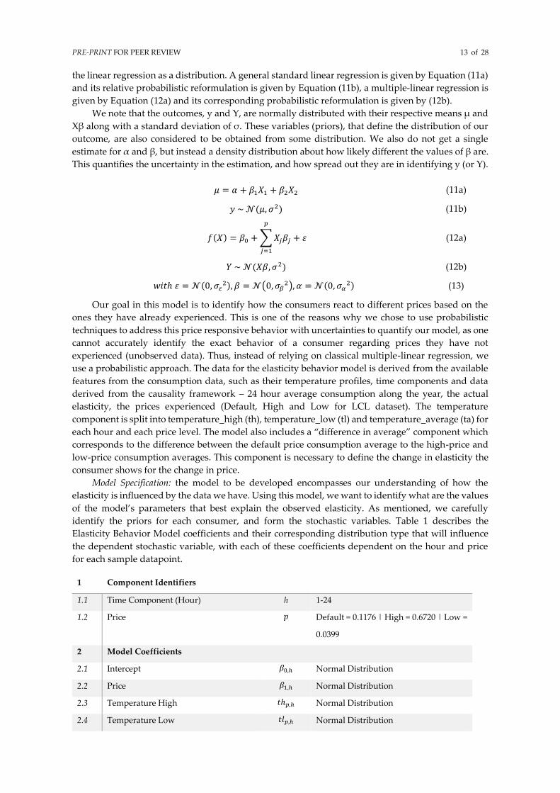
Model Specification: the model to be developed encompasses our understanding of how the
elasticity is influenced by the data we have. Using this model, we want to identify what are the values
of the model’s parameters that best explain the observed elasticity. As mentioned, we carefully
identify the priors for each consumer, and form the stochastic variables. Table 1 describes the
Elasticity Behavior Model coefficients and their corresponding distribution type that will influence
the dependent stochastic variable, with each of these coefficients dependent on the hour and price
for each sample datapoint.
1 Component Identifiers
1.1 Time Component (Hour) h 1-24
1.2 Price 𝑝 Default = 0.1176 | High = 0.6720 | Low =
0.0399
2 Model Coefficients
2.1 Intercept 𝛽0,ℎ Normal Distribution
2.2 Price 𝛽1,ℎ Normal Distribution
2.3 Temperature High 𝑡ℎ𝑝,ℎ Normal Distribution
2.4 Temperature Low 𝑡𝑙𝑝,ℎ Normal Distribution

PRE-PRINT FOR PEER REVIEW 14 of 28
2.5 Temperature Average 𝑡𝑎𝑝,ℎ Normal Distribution
2.6 Average Consumption 𝑦𝑎𝑣𝑔𝑝 Normal Distribution
2.7 Difference in consumption 𝑦𝑑𝑖𝑓𝑓𝑝 Normal Distribution
2.8 Observed Elasticity likelihood
(dependent variable)
𝑦 Student-T distribution
2.9 Degrees of freedom 𝜈 Uniform distribution
2.10 Standard Deviation 𝜎 Exponential distribution
Table 1. Elasticity Behaviour Model Components
The Student-T prior for the observed elasticity (dependent variable) y is considered instead of a
normal distribution, because it is better at handling outliers as it has a longer tail. From Figures 8,
and 9, we can see that our elasticity data has a significant amount of datapoints in the tail end of the
distribution, and it is pertinent to understand the elastic behavior of the consumers under all
conditions. Using the student-t distribution indicates our model to incorporate these outliers also as
data points to consider as they are not indicators of data abnormality. The Student’s T log-likelihood
of a normal variable (x) with gamma (Γ) distributed precision is given by (14), where the scalar
variable μ denotes the mean of the stochastic variable from our model (elasticity), ν degree of freedom
with a uniform distribution between 0 and 1, and λ given by the standard deviation (σ) with an
exponential log-likelihood.
𝑦 = 𝑓(𝑥 | 𝜇, 𝜆, 𝜈) = Γ (
𝜈 + 12
)
Γ (𝜈2
)(
𝜆
𝜋𝜈)
12⁄
[1 +𝜆(𝑥 − 𝜇)2
𝜈]
−𝜈+1
2
(14)
Figure 8 Grouping of elasticity values for all consumers for each hour under the high DR price

PRE-PRINT FOR PEER REVIEW 15 of 28
Figure 9 Grouping of elasticity values for all consumers for each hour under the low DR price
The mean 𝜇 (stochastic variable) of Equation (14) is the main component of our elasticity model
that describes the prior distributions over the observed data to link them with the response variable
𝑦. We also are specifically interested in whether different hours actually have different relationships
(slope) and different intercepts. This way, we can have the aggregated mean (𝜇) for all hours, as well
as individual hours, for every price along the distribution. Using Equation (15), we estimate the
probability distribution of 𝛽0 and 𝛽1 for each hour (note that all components are indexed for each
price). We also use a 𝑝𝑟𝑖𝑐𝑒2 and 𝑝𝑟𝑖𝑐𝑒3 terms to help with the model convergence.
𝜇 = 𝛽0,ℎ + 𝛽1,ℎ(𝑝𝑟𝑖𝑐𝑒)2 + 𝛽1,ℎ(𝑝𝑟𝑖𝑐𝑒)3 + 𝑡ℎ𝑝,ℎ(𝑇𝑒𝑚𝑝_ℎ𝑖𝑔ℎ) + 𝑡𝑙𝑝,ℎ(𝑇𝑒𝑚𝑝_𝑙𝑜𝑤) +
𝑡𝑎𝑝,ℎ(𝑇𝑒𝑚𝑝_𝑎𝑣𝑔) + 𝑦𝑎𝑣𝑔𝑝(𝑐𝑜𝑛𝑠𝑢𝑚𝑝𝑡𝑖𝑜𝑛_𝑎𝑣𝑔 ∗ ℎ𝑜𝑢𝑟) +
𝑦𝑑𝑖𝑓𝑓𝑝(𝑐𝑜𝑛𝑠𝑢𝑚𝑝𝑡𝑖𝑜𝑛_𝑑𝑖𝑓𝑓𝑒𝑟𝑒𝑛𝑐𝑒 ∗ ℎ𝑜𝑢𝑟)
(15)
4.2 Numerical Results
Similar to the Dirichlet-model, we implemented this Elasticity Behavior model using MCMC in
PYMC for 2000 samples (increasing the number of samples increases computation time, 2000 was
chosen as we had convergence already). Our model draws 2000 samples from the posterior in parallel
computing (2000 * 4 for a 4-core machine). We adjusted the model to use the first set of 1000 samples
as tuning samples to learn from, and the inferences are made only after the first set of 1000 samples
are used.
Model data contains the components responsible to make the desirable outcome 𝑦 for each hour
and each price, making it a dataset with 72 outcomes for every consumer. The posterior plot for
consumer D0346’s model components is given in Figures 10, 11 and 12. They describe the marginal
posterior distribution for the stochastic variables for each hour running from b_0 0 to b_0 23 for
coefficient 𝛽0 stacked on top of each other and b_1 0 to b_1 23 for coefficient 𝛽1 also stacked on top
of each other. These Figures summarize the posterior distributions of the parameters (from the
provided prior distributions and hyper-parameters) and present a 95% credible interval and the
posterior mean. The plots below are constructed with the 2000 samples from each of the 4-cores
(chains), pooled together. By looking at Figure 11 and 12, we also see that the marginals for 𝛽0 and
𝛽1 have distinctive differences in their values between hours, compared to the other model
components shown in Figure 10. This is the specific reason why we chose to incorporate hourly
changes to the intercept and price in our model. The more the measurements per hour (more than 72
outcomes), the higher will be our confidence in estimating the posterior density distribution. Looking
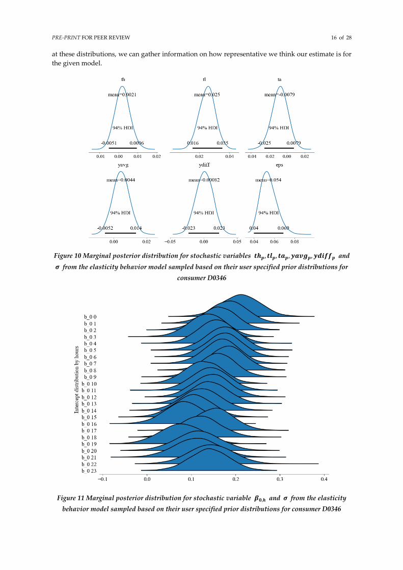
PRE-PRINT FOR PEER REVIEW 16 of 28
at these distributions, we can gather information on how representative we think our estimate is for
the given model.
Figure 10 Marginal posterior distribution for stochastic variables 𝒕𝒉𝒑, 𝒕𝒍𝒑, 𝒕𝒂𝒑, 𝒚𝒂𝒗𝒈𝒑, 𝒚𝒅𝒊𝒇𝒇𝒑 and
𝝈 from the elasticity behavior model sampled based on their user specified prior distributions for
consumer D0346
Figure 11 Marginal posterior distribution for stochastic variable 𝜷𝟎,𝒉 and 𝝈 from the elasticity
behavior model sampled based on their user specified prior distributions for consumer D0346

PRE-PRINT FOR PEER REVIEW 17 of 28
Figure 12 Marginal posterior distribution for stochastic variable 𝜷𝟏,𝒉 and 𝝈 from the elasticity
behavior model sampled based on their user specified prior distributions for consumer D0346
From the obtained traces containing the family of posteriors sampled for each consumer,
conditioned on the observations, we can plot the regression lines to compare them with their mean
and uncertainty (95% elasticity quantile). We plot the regression lines for some consumers in Figure
13 that show the estimated elasticity behavior measurements for different prices.
At this point, we must understand that our model derived these distributions based on 3 prices
that the consumers experienced during the recorded LCL DR program. In case we have a scenario
where consumers have experienced many price signals, for example dynamic DR tariffs, then this
model can be replaced with a comprehensive behavior model to get a better fit and estimate. This is
true as we will have more data points for identifying better behavior pattern.

PRE-PRINT FOR PEER REVIEW 18 of 28
Figure 13 Sampled range of posterior regression lines from the elasticity behaviour model for
consumers D0346, D0767, D0644 and D0557
These regression lines are formed from the posterior predictive distribution recreating the data
based on the parameters found at different moments in the chain. The recreated or predicted values
are subsequently compared to the real data points. The thick red line represents the mean estimate of
the regression line of the individual consumer and the thinner blue lines are the individual samples
from the posterior that give us a perspective of uncertainty in our estimates. The elasticity behavior
model can be used to identify how a consumer reacts to different prices for a given time-period and
temperature conditions.

PRE-PRINT FOR PEER REVIEW 19 of 28
(a) (b)
(c) (d)
Figure 14 Average elasticity profile compared to the actual elasticity profile from the causality
model, for all 72 response variables (y) for consumers (a) D0346, (b) D0767, (c) D0644 and (d) D0557
Figure 14 compares our elasticity behavior model’s mean estimates with the actual elasticity
provided by the causality model for each 72 response variables and depicts our model convergence.
The 1st 24 response variables (0-23) correspond to the default DR price - 0.1176 £/kWh, response
variables 24 to 47 correspond to high DR price - 0.6720 £/kWh, and response variables 48 to 71
correspond to low DR price - 0.0390 £/kWh. It should be noted that our model assumes that all the
prices considered in these posterior estimates are new DR prices, and this is the reason we see smaller
deviations in our modelled average elasticity in the first 24 response variables (which correspond to
the default DR price). The posterior probability distribution for each of the 72 response variables (𝑦)
for our estimates of elasticity with the elasticity behavior model is shown in Figure 15 for consumer
D0346.

PRE-PRINT FOR PEER REVIEW 20 of 28
Figure 15 Posterior probability density distribution of elasticity for each of the 72 response
variables obtained by the elasticity behaviour model
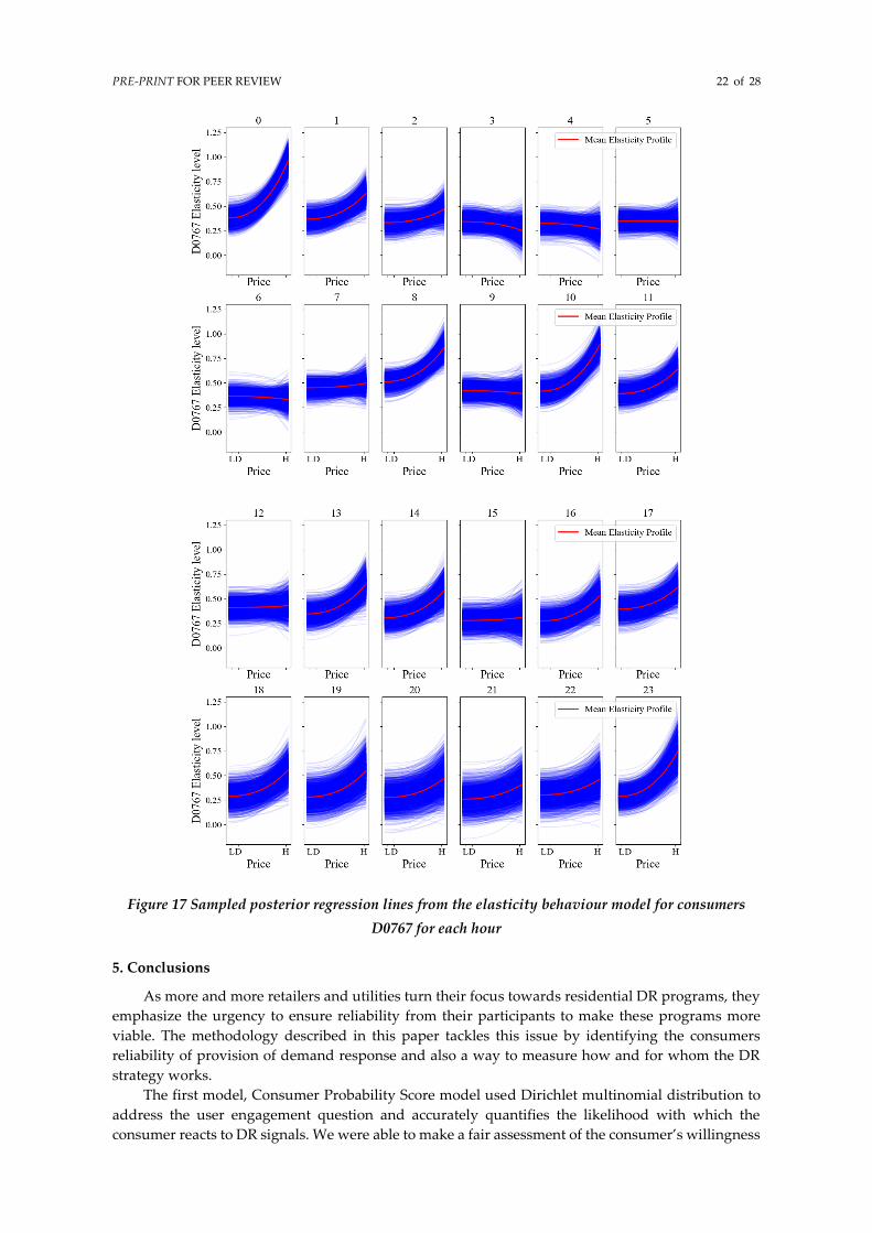
The model was constructed to identify the effects from the marginals for 𝛽0 and 𝛽1 as they
have distinctive differences in their values between hours of the day (Figure 11 and 12). From our
causality framework, it is also evident that the consumers behave differently for different hours of
the day. To show this pattern in our estimated behavioral model, we analyzed the impact of price
change on elasticity for each hour as shown in Figures 16 and 17. This gives us an inference that
consumer D0346 shows a typical elasticity profile (expected by utilities or retailers) where the
consumer is quite price responsive the early hours of the day. During the rest of the hours, namely
on midday and late-night hours, this consumer’s behavior is quite inelastic.
Compared to this, consumer D0767 seems to have a very price responsive behavior throughout
the day with one of the most elastic periods being hour 10:00 am of the day. Typically, this cannot be
seen in a general price responsive model, where they will follow the elasticity profile shown by
consumer D0346 as a general price responsive behavior for all their clients. This elasticity behavior

PRE-PRINT FOR PEER REVIEW 21 of 28
model is constructed in such a way that the utility or retailer can tune the features enumerated in
Table 1 to accurately identify the elasticity behavior profile for each consumer and use the consumer
probability score model to group and identify the exact probability of consumer responsiveness to
the new DR price offers. This way, the utility or retailers can know how a new DR strategy can
perform amongst its clients with greater reliability.
Figure 16 Sampled posterior regression lines from the elasticity behaviour model for consumers
D0346 for each hour
PRE-PRINT FOR PEER REVIEW 22 of 28
Figure 17 Sampled posterior regression lines from the elasticity behaviour model for consumers
D0767 for each hour
5. Conclusions
As more and more retailers and utilities turn their focus towards residential DR programs, they
emphasize the urgency to ensure reliability from their participants to make these programs more
viable. The methodology described in this paper tackles this issue by identifying the consumers
reliability of provision of demand response and also a way to measure how and for whom the DR
strategy works.
The first model, Consumer Probability Score model used Dirichlet multinomial distribution to
address the user engagement question and accurately quantifies the likelihood with which the
consumer reacts to DR signals. We were able to make a fair assessment of the consumer’s willingness

PRE-PRINT FOR PEER REVIEW 23 of 28
to participate in DR events. Using the LCL dataset, we conclude that consumers who show low
variations in response probability are more reliable and less risky to be considered for targeted DR
signals rather than consumers who have high variations in their responses. Regarding the second
model, the Elasticity Behavior Model uses a Bayesian probabilistic approach and identifies the actual
load adjustment an individual contracted DR client provides for different price levels they can
experience. This allows the retailers to understand the full potential of consumption elasticity
behavior from their contracted clients from the already available data without the need to send new
price signals and strategies to the same consumers. Thus, this work provides a holistic approach to
capture the customers uncertainty in modeling the consumer selection problem for new targeted DR
strategies.
The framework proposed in this paper was developed with the goal for it to be scalable. This
framework can be effectively extended to other consumers such as small and medium service
buildings and even community buildings where extracting a larger amount of controlled and
aggregated services can become highly effective. With predicting a consumer’s kWh consumption
becoming a more widely and common study, using the elasticity measure as a feature for such model
would help the model in achieving higher accuracies. This has already been proved by a research
work [43, 44] where the authors, using Conditional Variational Autoencoders, generate daily
consumption profiles of consumer segmented in different clusters (based on response to electricity
tariff). We used dynamic Time-Of-Use (TOU) tariffs for our elasticity behavior model. A continuous
dynamic pricing such as RTP tariffs can bring more granularity and better insights into a consumer’s
consumption behavior. Extending this work towards this direction would enable understanding
what is the best-fit pricing strategy for residential consumers before hitting elasticity saturation and
eventual indifference towards price changes.
Appendix A
6. Causality Inference Algorithms
Data analysis and causal inference for our framework was performed using Robin’s g-method
to estimate the average consumption and elasticity for each hour. The Robin g-method enables the
identification and estimation of the effects of generalized treatment, exposure, and intervention
plans. It provides consistent estimates of contrasts of average potential outcomes under a less
restrictive set of identification conditions than standard regression models [45]. The estimated
consumption elasticity is then pooled together with all clients and ranked by hours. The modeled
approach helps in making a fair estimate of whether the consumers introduced any changes to their
consumption based on DR signals, as it can differentiate between a normal consumption and a DR
stimulated consumption. The algorithm used in our consumer elasticity model uses the parametric
g-formula (as the causal effect estimator) and arbitrary machine learning estimators to analyze and
plot causal effects [46]. Causal effect refers to the distribution or conditional expectation of Y given
X, controlling for an admissible set of covariates, Z, to make the effect identifiable. Covariates Z are
exogenous variables whose value is determined outside the model and is imposed on the developed
model. In our analysis (simple depiction in Figure A.1), X, being price, and Z, being time, are indeed
correlated; more precisely, they will be statistically dependent.
Figure A.1 Causal Graph of X and Y related by a common cause
PRE-PRINT FOR PEER REVIEW 24 of 28
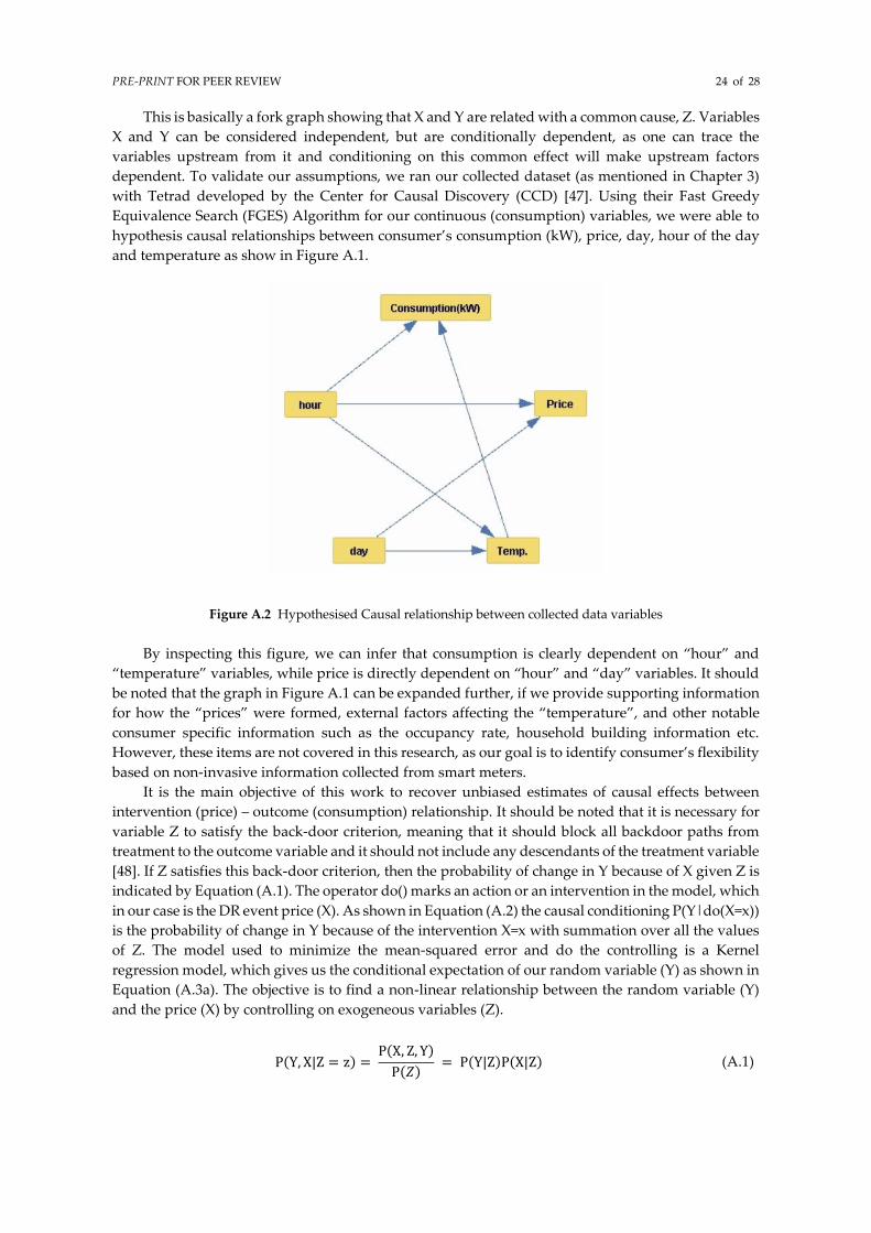
This is basically a fork graph showing that X and Y are related with a common cause, Z. Variables
X and Y can be considered independent, but are conditionally dependent, as one can trace the
variables upstream from it and conditioning on this common effect will make upstream factors
dependent. To validate our assumptions, we ran our collected dataset (as mentioned in Chapter 3)
with Tetrad developed by the Center for Causal Discovery (CCD) [47]. Using their Fast Greedy
Equivalence Search (FGES) Algorithm for our continuous (consumption) variables, we were able to
hypothesis causal relationships between consumer’s consumption (kW), price, day, hour of the day
and temperature as show in Figure A.1.
Figure A.2 Hypothesised Causal relationship between collected data variables
By inspecting this figure, we can infer that consumption is clearly dependent on “hour” and
“temperature” variables, while price is directly dependent on “hour” and “day” variables. It should
be noted that the graph in Figure A.1 can be expanded further, if we provide supporting information
for how the “prices” were formed, external factors affecting the “temperature”, and other notable
consumer specific information such as the occupancy rate, household building information etc.
However, these items are not covered in this research, as our goal is to identify consumer’s flexibility
based on non-invasive information collected from smart meters.
It is the main objective of this work to recover unbiased estimates of causal effects between
intervention (price) – outcome (consumption) relationship. It should be noted that it is necessary for
variable Z to satisfy the back-door criterion, meaning that it should block all backdoor paths from
treatment to the outcome variable and it should not include any descendants of the treatment variable
[48]. If Z satisfies this back-door criterion, then the probability of change in Y because of X given Z is
indicated by Equation (A.1). The operator do() marks an action or an intervention in the model, which
in our case is the DR event price (X). As shown in Equation (A.2) the causal conditioning P(Y|do(X=x))
is the probability of change in Y because of the intervention X=x with summation over all the values
of Z. The model used to minimize the mean-squared error and do the controlling is a Kernel
regression model, which gives us the conditional expectation of our random variable (Y) as shown in
Equation (A.3a). The objective is to find a non-linear relationship between the random variable (Y)
and the price (X) by controlling on exogeneous variables (Z).
P(Y, X|Z = z) = P(X, Z, Y)
P(𝑍) = P(Y|Z)P(X|Z) (A.1)

PRE-PRINT FOR PEER REVIEW 25 of 28
P(Y|do(X = x)) = ∑ P(Y|X, Z)P(Z)
Z
(A.2)
E(Y|x) = ∑ YP(Y|x)
Y
= ∑ YP(Y|X, Z)P(Z)
Y,Z
(A.3a)
𝑚(𝑥) = 𝐸[𝑌|𝑑𝑜(𝑋 = 𝑥)] = ∑ 𝐸[𝑌|𝑋, 𝑍]𝑃(𝑍)
𝑍
(A.3b)
E[Y|(X𝑗)] = ∑1
N
24
ℎ=1
∑ E[Y|X𝑗 , (Zℎ𝑖 , Z2i, Z3i, Z4i)]
N
i=1
(A.4)
Z − Interval = 𝐸[𝑌|𝑋, 𝑍] ± 𝑧𝛼2⁄ (𝜎) (A.5)
The model used by default to minimize the mean-squared error and do the controlling is a
Kernel regression model which gives us the conditional expectation as shown in Equation (A.3b). The
causal dataframe helps in finding the true dependency between the X (price) and Y (consumption)
with the confounders as the calendar variables, we consider X: price, Y: consumption and Z: calendar
variables (hour - Z1, day - Z2 and week - Z3). For every hour (Z1), the causal effect of (X) on (Y) is
obtained for each DR price (Xj) with constant (Z1) and variable (Z2 & Z3) with i=1 to N running over
all data points as shown in Equation (A.4). These calendar variables are confounders that have effects
on both price and consumption. The causal analysis model works by controlling the Z variables when
trying to estimate the effect of variable X on a continuous variable Y (Equation A.4). The model
returns Y estimates (E[y]) at each X=x value for every Z and provides the upper and lower average
consumption limits of the Y variable, which is used to determine the average elasticity. The upper
and the lower consumption limits of the average Y variable (for each price) is the z-intervals
calculated using the confidence levels (CI = 95% for our model). The z-interval for our consumption
average Y estimates is shown in Equation (A.5) where 𝑧𝛼 2⁄ is the alpha level’s z-score for a two tailed
test (based on the value of CI) and σ is the standard deviation of our average Y estimate. The
constructed causality model is then used to provide the estimates for each consumer demand on each
hour for each price.
Funding: This work was financially supported by the European Union’s Horizon 2020 research and innovation
programme, under Grant agreement No 857237 (InterConnect—Interoperable Solutions Connecting Smart
Homes, Buildings and Grid). Kamalanathan Ganesan was also supported by the European Social Fund (FSE)
through NORTE 2020 under PhD Grant NORTE-08-5369-FSE-000043. The sole responsibility for the content lies
with the authors. It does not necessarily reflect the opinion of the CNECT or the European Commission (EC).
CNECT or the EC are not responsible for any use that may be made of the information contained therein.
Conflicts of Interest: The authors declare no conflict of interest. The funders had no role in the design of the
study; in the collection, analyses, or interpretation of data; in the writing of the manuscript, or in the decision to
publish the results.
References
1. Belgium, C., Impact Assessment Support Study on Downstream Flexibility, Demand Response and Smart
Metering. 2016, European Commission.

PRE-PRINT FOR PEER REVIEW 26 of 28
2. Parrish, B., R. Gross, and P. Heptonstall, On demand: Can demand response live up to expectations in
managing electricity systems? Energy Research & Social Science, 2019. 51: p. 107-118.
3. Abi Ghanem, D. and S. Mander, Designing consumer engagement with the smart grids of the future: bringing
active demand technology to everyday life. Technology Analysis and Strategic Management, 2014. 26: p.
1163-1175.
4. Kim, J.-H. and A. Shcherbakova, Common failures of demand response. Energy, 2011. 36(2): p. 873-880.
5. Gottwalt, S., et al., Demand side management—A simulation of household behavior under variable prices.
Energy Policy, 2011. 39(12): p. 8163-8174.
6. Australia, E.C., Power Shift Final Report, E.C. Australia, Editor. 2020.
7. Finn, P., M. O’Connell, and C. Fitzpatrick, Demand side management of a domestic dishwasher: Wind energy
gains, financial savings and peak-time load reduction. Applied Energy, 2013. 101: p. 678-685.
8. Afzalan, M. and F. Jazizadeh, Residential loads flexibility potential for demand response using energy
consumption patterns and user segments. Applied Energy, 2019. 254: p. 113693.
9. Lopes, J. and P. Agnew. Florida Power & Light: Residential Thermostat Load Control Pilot Project Evaluation.
ACEEE.
10. Navigant, Evaluation of Time-of-Use Pricing Pilot, O.E. Board, Editor. 2008, Ontario Energy Board.
11. George, S., M. Perry, and P. Malaspina, 2013 Load Impact Evaluation for Pacific Gas and Electric Company's
SmartAC Program. 2011.
12. Ericson, T., Direct load control of residential water heaters. Energy Policy, 2009. 37(9): p. 3502-3512.
13. Herter, K., P. McAuliffe, and A. Rosenfeld, An exploratory analysis of California residential customer
response to critical peak pricing of electricity. Energy, 2007. 32(1): p. 25-34.
14. Zhou, D., M. Balandat, and C. Tomlin, Residential Demand Response Targeting Using Machine Learning
with Observational Data. 2016.
15. Karangelos, E. and F. Bouffard. Integrating Demand Response into agent-based models of electricity markets.
in 2012 50th Annual Allerton Conference on Communication, Control, and Computing (Allerton). 2012.
16. Gils, H.C., Assessment of the theoretical demand response potential in Europe. Energy, 2014. 67: p. 1-18.
17. SEDC, Explicit Demand Response in Europe - mapping the markets in 2017. 2017.
18. Directive 2018/2001/EU on the promotion of the use of energy from renewable sources, O.J.o.t.E. Union, Editor.
2018.
19. Directive 2019/944/EU on the internal electricity market, O.J.o.t.E. Union, Editor. 2019.
20. Ahmed, S. and F. Bouffard, Building load management clusters using reinforcement learning. 2017. 372-377.
21. Haben, S., C. Singleton, and P. Grindrod, Analysis and Clustering of Residential Customers Energy
Behavioral Demand Using Smart Meter Data. IEEE Transactions on Smart Grid, 2016. 7(1): p. 136-144.
22. Zhou, K.-l., S.-l. Yang, and C. Shen, A review of electric load classification in smart grid environment.
Renewable and Sustainable Energy Reviews, 2013. 24: p. 103-110.
23. Kwac, J., J. Flora, and R. Rajagopal, Household energy consumption segmentation using hourly data. IEEE
Transactions on Smart Grid, 2014. 5(1): p. 420-430.
24. Kwac, J., J. Flora, and R. Rajagopal, Lifestyle Segmentation Based on Energy Consumption Data. IEEE
Transactions on Smart Grid, 2018. 9(4): p. 2409-2418.
25. Wang, Y., et al., Clustering of Electricity Consumption Behavior Dynamics Toward Big Data Applications.
IEEE Transactions on Smart Grid, 2016. 7(5): p. 2437-2447.
26. Tsekouras, G.J., et al., A pattern recognition methodology for evaluation of load profiles and typical days of large
electricity customers. Electric Power Systems Research, 2008. 78(9): p. 1494-1510.

PRE-PRINT FOR PEER REVIEW 27 of 28
27. McLoughlin, F., A. Duffy, and M. Conlon, A clustering approach to domestic electricity load profile
characterisation using smart metering data. Applied Energy, 2015. 141: p. 190-199.
28. Biswas, S. and S.A. Abraham. Identification of Suitable Consumer Groups for Participation in Demand
Response Programs. in 2019 IEEE Power & Energy Society Innovative Smart Grid Technologies Conference
(ISGT). 2019.
29. Chicco, G. and I. Ilie, Support Vector Clustering of Electrical Load Pattern Data. IEEE Transactions on Power
Systems, 2009. 24(3): p. 1619-1628.
30. Piao, M., et al., Subspace Projection Method Based Clustering Analysis in Load Profiling. IEEE Transactions
on Power Systems, 2014. 29(6): p. 2628-2635.
31. Teeraratkul, T., D. O’Neill, and S. Lall, Shape-Based Approach to Household Electric Load Curve Clustering
and Prediction. IEEE Transactions on Smart Grid, 2018. 9(5): p. 5196-5206.
32. Shahzadeh, A., A. Khosravi, and S. Nahavandi. Improving load forecast accuracy by clustering consumers
using smart meter data. in 2015 International Joint Conference on Neural Networks (IJCNN). 2015.
33. Newsham, G.R., B.J. Birt, and I.H. Rowlands, A comparison of four methods to evaluate the effect of a utility
residential air-conditioner load control program on peak electricity use. Energy Policy, 2011. 39(10): p. 6376-
6389.
34. Herter, K. and S. Wayland, Residential response to critical-peak pricing of electricity: California evidence.
Energy, 2010. 35(4): p. 1561-1567.
35. Ganesan, K., J.T. Saraiva, and R.J. Bessa. Using Causal Inference to Measure Residential Consumers Demand
Response Elasticity. in 2019 IEEE Milan PowerTech. 2019.
36. Ganesan, K., J. Tomé Saraiva, and R.J. Bessa, On the Use of Causality Inference in Designing Tariffs to
Implement More Effective Behavioral Demand Response Programs. Energies, 2019. 12(14).
37. Schofield, J.R., Carmichael, R., Tindemans, S., Bilton, M., Woolf, M., Strbac, G., Low Carbon London
Project: Data from the Dynamic Time-of-Use Electricity Pricing Trial, 2013, L.P.N. PLC, Editor. 2016: UK
Data Service.
38. Underground, W., Historic Weather Data. 2014.
39. Kim, Y.-S. and J. Srebric, Impact of occupancy rates on the building electricity consumption in commercial
buildings. Energy and Buildings, 2017. 138: p. 591-600.
40. Homan, M.D. and A. Gelman, The No-U-turn sampler: adaptively setting path lengths in Hamiltonian Monte
Carlo. J. Mach. Learn. Res., 2014. 15(1): p. 1593–1623.
41. Duane, S., et al., Hybrid Monte Carlo. Physics Letters B, 1987. 195(2): p. 216-222.
42. Minka, T.P., Estimating a Dirichlet distribution, in Technical report Microsoft Research. 2003, Microsoft
Research.
43. Brégère, M., Stochastic bandit algorithms for demand side management. 2020, Université Paris-Saclay.
44. Brégère, M. and R.J. Bessa, Simulating Tariff Impact in Electrical Energy Consumption Profiles With
Conditional Variational Autoencoders. IEEE Access, 2020. 8: p. 131949-131966.
45. Naimi, A.I., S.R. Cole, and E.H. Kennedy, An introduction to g methods. International journal of
epidemiology, 2017. 46(2): p. 756-762.
46. Keil, A.P., et al., The parametric g-formula for time-to-event data: intuition and a worked example.
Epidemiology, 2014. 25(6): p. 889-97.
47. Cooper, G.F., et al., The center for causal discovery of biomedical knowledge from big data. Journal of the
American Medical Informatics Association, 2015. 22(6): p. 1132-1136.

PRE-PRINT FOR PEER REVIEW 28 of 28
48. Neuberg, L.G., CAUSALITY: MODELS, REASONING, AND INFERENCE, by Judea Pearl, Cambridge
University Press, 2000. Econometric Theory, 2003. 19(4): p. 675-685.