article in press - climatic research unit - university of east anglia

G

D

O

CS

TC

a

ARA

KTDSSRS

I

rfccuslttumbTiTmtrfiB

1h

ARTICLE IN PRESS Model

ENDRO-25256; No. of Pages 14

Dendrochronologia xxx (2013) xxx– xxx

Contents lists available at ScienceDirect

Dendrochronologia

j ourna l ho me page: www.elsev ier .com/ locate /dendro

riginal article

RUST: Software for the implementation of Regional Chronologytandardisation: Part 1. Signal-Free RCS

homas M. Melvin ∗, Keith R. Briffalimatic Research Unit, School of Environmental Sciences, University of East Anglia, Norwich NR4 7TJ, UK

r t i c l e i n f o

rticle history:eceived 16 February 2013ccepted 5 June 2013

eywords:ree rings

a b s t r a c t

This is the first of a two-part description of a new software tool CRUST (Climatic Research UnitStandardisation of Tree-ring data). This program has been designed primarily to allow the convenient,routine application of “Signal-Free Regional Chronology Standardisation” (SF RCS) to different types oftree-ring data. The program also enables the use of other popular standardisation methods. A series ofexperiments is described in which the ability of simple RCS and SF RCS to recover known tree-growth

endroclimatologytandardisationoftwareCSignal-Free

forcing signals is tested. In the comparatively rare situation where many sub-fossil data are distributedover a wide time range and there is no slope in the overall common-growth forcing signal, simple RCSis satisfactory. Simple RCS produces distortion in all other examples explored here. SF RCS is superior tosimple RCS and in all cases examined. SF RCS works well except when the span of starting dates of sampletrees is too narrow, a situation for which a test is available. Based on the results of the tests explored here,

ree R

igt

dlaabEoaRuiosogps

we conclude that Signal-F

ntroduction

In dendroclimatology the changes seen in series of annual tree-ing measurements are used to identify changes in the commonorcing of tree growth over time and in some circumstances thishanging growth rate of trees is used as a “proxy” for changinglimate. Tree-ring measurements also contain variations that arenrelated to climate: caused by biological and mechanical con-traints on tree growth encountered as the tree becomes older andarger. These changes are referred to as the “age-related-growthrend” or the “expected growth curve” i.e. the changes in a series ofree-ring measurements throughout the life of a tree growing in annchanging climate. These changes need to be removed from theeasurements in order to better isolate growth variations caused

y climate variability (Fritts, 1976, Chapter 6, Cook et al., 1990).he process of removing the age-related growth trend (detrend-ng) to produce indices of tree growth is called “standardisation”.raditional methods of detrending involved fitting a curve to theeasurement series and removing the variance represented by

he fitted curve. Depending on the longevity of trees, this processemoves substantial, and in many cases all, long-timescale variance

Please cite this article in press as: Melvin, T.M., Briffa, K.R., CRUST: SoftwaPart 1. Signal-Free RCS. Dendrochronologia (2013), http://dx.doi.org/10.10

rom a chronology and imposes serious low-frequency limitationsn subsequent dendroclimatic reconstructions (Cook et al., 1995;riffa et al., 1996). In order to overcome this frequency limitation

∗ Corresponding author. Tel.: +44 01603 593161; fax: +44 01603 507784.E-mail address: [email protected] (T.M. Melvin).

aticdTs

125-7865/$ – see front matter © 2013 Elsevier GmbH. All rights reserved.ttp://dx.doi.org/10.1016/j.dendro.2013.06.002

CS should be used as the standard method of RCS processing.© 2013 Elsevier GmbH. All rights reserved.

t is necessary to estimate and remove the expected non-climaterowth rate change in tree-ring measurements independently ofhe growth of individual trees.

Regional Curve Standardisation (RCS) was introduced to den-roclimatology (Briffa et al., 1992) to overcome the frequency

imitation of curve-fitting standardisation. It does so by using theverage of the measurements of the rings of all trees at each ringge as the expected growth value for each individual tree. RCS haseen used in various forms for nearly a century (Huntington, 1914;rlandsson, 1936; Briffa et al., 1992; Esper et al., 2002). A reviewf the background and implementation of RCS is provided in Briffand Melvin (2011). There are a number of problems associated withCS and these may to some extent have prevented the widespreadptake of this method. In RCS, as normally implemented to date, it

s assumed that any influence of the common signal on the shapef the RCS curve will be removed by the process of realigning mea-urement series by ring age and averaging. In effect, large numbersf sub-fossil (or historical or archaeologically sourced) trees whichrew over widely differing periods are needed for this averagingrocess to be effective (Briffa et al., 1992, 1996). This requirementeverely restricts the application of RCS to sites with substantialmounts of sub-fossil samples. Melvin and Briffa (2008) introducedhe concept of “signal-free” standardisation where the detrend-ng curve is estimated using measurement data from which the

re for the implementation of Regional Chronology Standardisation:16/j.dendro.2013.06.002

ommon growth-forcing signal has been removed i.e. where theetrending curve is not distorted by the effect of climate forcing.his method was originally described in the context of curve-fittingtandardisation. However, the signal-free method can also be used

dx.doi.org/10.1016/j.dendro.2013.06.002


http://www.sciencedirect.com/science/journal/11257865

http://www.elsevier.com/locate/dendro

mailto:[email protected]


ING Model

D

2 rochr

tteiulHoit

auomtbaai

B

P

tsmtsmmcitrtitatRou

S

acpchamamytvvmm

ciov

A

omBt

et

tioatwttrdhofuciiocu

nOdctsotw

ARTICLEENDRO-25256; No. of Pages 14

T.M. Melvin, K.R. Briffa / Dend

o create an RCS curve that is not biased by the common signal andhis largely reduces the need for many sub-fossil data. The ben-fits and limitations of the application of the signal-free methodn RCS, particularly for standardising “living tree” data are eval-ated and discussed here. Another factor that has, up until now,

imited the uptake of RCS is the lack of widely available software.ere we introduce CRUST (Climatic Research Unit Standardisationf Tree-ring data): a software package that can be used for routinemplementation of, and experimentation with, SF RCS and otherypes of tree-ring standardisation.

In the two companion papers, of which this is Part 1, we describe number of RCS implementation options. Herein, we focus on these of signal-free RCS (SF RCS) and describe the basic functionsf CRUST. In Part 2, we focus on other aspects of the use of CRUST,aking specific implementation recommendations and suggesting

he use of various diagnostic procedures when using SF RCS. Weegin here by providing some background to the concepts of simplend SF RCS. We then describe the implementation of RCS in CRUSTnd describe a number of examples selected to demonstrate howt performs in practice.

ackground

reservation of long-timescale variance

We define three frequency ranges, relative to the lengths ofree-ring series; firstly, low-frequency chronology variance is con-idered to be at timescales beyond the age of a tree; secondly,edium-frequency variance spans time scales from decades to

he age of a tree; and thirdly, high-frequency variance is that atub-decadal timescales. When using curve-fitting standardisationethods the mean of each series of tree indices is set to 1.0. Theean of the chronology indices over the length of a tree will be

lose to 1.0 and there will be no low-frequency variance in result-ng chronologies (Cook et al., 1995). When a sloping line is fittedo series of measurements the slope, over the life of the tree, isemoved from the resulting tree indices, further limiting the reten-ion of medium-frequency variance. In RCS, the value of each treendex is set relative to the value of the RCS curve at that ring age andhe average value of each index series can, therefore, vary consider-bly. The low-frequency variance of an RCS chronology is based onhe changing value of the mean growth rate of trees over time. InCS, the slope of each series of tree indices is set relative to the slopef the RCS curve and the resulting index series for a tree can slopep or down enabling RCS to preserve medium-frequency variance.

imple RCS method

It is possible to implement RCS in different ways and variouspproaches or refinements have been explored to date (see dis-ussion in Briffa and Melvin, 2011). We use some commonly usedrocedures to define “simple RCS” which forms the basis for theomparisons with alternative implementations of RCS discussedere. In simple RCS all series of ring measurements for a site areligned by cambial age and the arithmetic average of measure-ents is used to produce a curve of mean measurement by cambial

ge. When available, “pith-offset” estimates are used in the assess-ent of ring age, otherwise the first ring is presumed to be the first

ear of tree growth. The “mean measurement by ring age” curveends to be noisy and needs to be smoothed. Here we use a time-


arying response spline (Melvin et al., 2007), to create a smoothlyarying RCS curve. This RCS curve is taken to represent the expectedeasurement value for each year of growth in an unvarying cli-ate. Each ring-width measurement is then divided by the RCS

ostt

PRESSonologia xxx (2013) xxx– xxx

urve value for its particular ring age to give a dimensionless treendex. These indices are fractional deviations. The arithmetic meanf all tree indices for a particular calendar year is the chronologyalue for that year.

conceptual RCS model

Melvin (2004, p. 53–56) describes a simple multiplicative modelf tree growth and adapts this model for use with the signal-freeethod in the context of curve-fitting standardisation (Melvin and

riffa, 2008). This can be described by a series of conceptual equa-ions:

Ring width = Expected growth * Chronology index * ErrorTree index = Ring measurement/Expected growthTree index = Chronology index * ErrorSF measurement = Ring measurement/Chronology indexSF measurement = Expected growth * Error.

When using curve-fitting standardisation methods, the meanrror over the life of a tree will be close to one and this error can bereated as random noise.

For practical purposes a ring growth model need only definehose factors that can be effectively isolated in analysis, with thenfluence of un-resolvable factors considered as part of the chronol-gy error. In RCS, “Expected Growth” is the RCS curve value for theppropriate ring age and low-frequency variance is preserved inhe mean value of each series of tree indices. If, for convenience,e ignore any uncertainty in the RCS curve itself we can consider

he RCS chronology error as composed of separate parts. Firstly,here is the medium- plus high-frequency error (equivalent to thatesulting from the use of curve-fitting methods). This arises fromifferences in series of tree indices which have been rescaled toave mean values that are equal to the mean of the chronologyver their common period and represented as fractional deviationsrom chronology values. Secondly, there is the low-frequency error,nique to RCS, which is the error (as fractional deviations) in ahronology created by averaging series of mean values for each tree.e. where for each tree all index values are replaced by the meanndex value. The medium- to high-frequency error is independentf that for low frequencies. In this discussion we are principallyoncerned with aspects of the low-frequency chronology and itsncertainty.

For the RCS growth model we can write:

Ring width = RCS curve value * Chronology index * Mean offset *ErrorTree index = Ring measurement/Expected growthTree index = Chronology index * Mean offset * Error.

These equations suggest the use of several techniques for diag-osing problems and for reducing bias in the use of RCS. “Meanffset” is a factor by which a series of indices from one tree must beivided in order to adjust its mean to be the same as the mean of thehronology over their common period. In a signal and noise context,he average of mean offsets for all tree-index series provides a mea-ure of the chronology error representing within-site variations inverall tree growth rates. This also provides a benchmark for inves-igating the degree of homogeneity in low-frequency growth ratesithin sites, or across groups of sites in a wider-regional chronol-


gy, and for comparing different growth rates as represented ineparate sample sources (e.g. sub-fossil, archaeological or livingree samples). The “noise” represented by mean offset needs to beaken into account in the assessment of low-frequency chronology


ING Model

D

rochr

sp

m

eytaatrc

U

ecgrtwctsAdcttpwfdiwu

I

tticmMfpcsfsahifrc

rSuvutwgcnm

adR

123

4

vRid

1

2345

67

tiS

E

odcrabrTe



ignal strength. This is discussed in the companion (Part 2) to thisaper.

For the RCS growth model we can define signal-free measure-ents:

SF measurement = Ring measurement/Chronology index.SF measurement = RCS curve value * Mean offset * Error.

Dividing a ring measurement by the chronology index gives anstimate of growth that might have occurred in an average climateear (a signal-free measurement). Dividing ring measurements byhe appropriate RCS curve value and multiplying by the value atnother ring age provides an estimate of the expected growth ratet that alternative ring age and enables conversion of all rings tohose “expected” for any specific ring age. This is useful in the explo-ation of the efficiency of using “multiple” rather than “single” RCSurves and is also discussed in Part 2.

sing the Signal-Free method with RCS

An example of how an RCS curve can be distorted by the pres-nce of common signal would be where the “old” section of the RCSurve was made up of average ring widths only from old trees thaterminated at a similar date. The RCS curve would contain varianceepresenting the common climate signal in ring widths from theserees in addition to the non-climatic, “biological” decline in ringidth. However, because the pattern and magnitude of chronology

ommon signal is known (or at least can be reasonably estimated ashe chronology variance), this signal can be removed from all mea-urement series by division, creating series of SF measurements.n RCS curve created from SF measurements (SF RCS curve) willisplay minimal influence from the long-timescale variance of theommon forcing signal. The signal-free method thus has the poten-ial to remove, or reduce, the need for large numbers of sub-fossilrees when constructing an RCS chronology. The CRUST programrovides a convenient way of implementing this approach. Heree describe the SF RCS and show how the existence of medium-

requency variance in the common forcing of tree growth canistort the shape of the simple RCS curve leading to systematic bias

n the (non-signal-free) RCS chronology when this is constructedith insufficient sub-fossil samples. We also demonstrate how these of the signal-free method can mitigate this problem.

mplementing the Signal-Free method

Chronology indices, as the mean of tree indices which are frac-ional deviations, represent the magnitude of common forcing ofree growth in each year as a fraction of the average value of treendices. Dividing each ring measurement by the appropriate-yearhronology index will remove the variance representing the com-on forcing of tree growth from each series of measurements.elvin and Briffa (2008), describe the application of the signal-

ree method in the context of “curve-fitting” standardisation. Therocess is applied iteratively. When applied in the case of RCS, ahronology is first produced using RCS standardisation. Each mea-urement value is then divided by the appropriate chronology valueor that year to produce a set of SF measurements. If the commonignal has been effectively removed from all measurement series,

chronology created by standardising these SF measurements willave virtually zero variance. This will not be achieved in the first


teration. The SF residual-chronology represents distortion arisingrom the effect of residual common signal on the RCS curve and isemoved from the chronology by multiplication i.e. SF residual-hronology times chronology. Therefore, the standardisation is

4s“e

PRESSonologia xxx (2013) xxx– xxx 3

epeated but this time using the SF measurements, creating a newF RCS curve and a SF residual-chronology. The process is repeatedntil the point where the SF residual-chronology has near-zeroariance. In practice, the magnitude of the variance of the SF resid-al chronology is roughly 20% of its value from the previous itera-ion. A zero-variance SF residual-chronology is considered to be onehere all values are within the range 1.0 ± 0.002. This is achieved

enerally within 4 or 5 iterations. At this point the “final” SF RCSurve is unaffected by the medium-frequency variance of the exter-al growth-forcing signal and when used to standardise the originaleasurement series will yield an optimum SF RCS chronology.In CRUST, an “RCS standardisation” procedure, which creates

n RCS chronology, is called repeatedly as part of the process ofeveloping a SF RCS chronology. We can therefore, summarise theCS process as follows:

RCS Standardisation:

. Average the measurement data into a mean curve by ring age.

. Smooth the RCS curve.

. Divide measurements by appropriate cambial age values of thesmoothed RCS curve to create tree indices.

. Average tree indices by calendar year to create the RCS chronol-ogy.

In CRUST, RCS standardisation allows a selection from thearious available implementation options e.g. using multipleCS curves, using diameter based RCS curves, using basal area

ncrement, or using robust means etc. (see Principal CRUST stan-ardisation options).

Signal-Free method:

. Set the SF measurement values to the original measurementvalues.

. Set all SF residual-chronology values to 1.0.

. Set all chronology values to 1.0.

. Divide SF measurements by the SF residual-chronology values.

. Create a SF residual-chronology using SF measurements with“RCS Standardisation” as above.

. Multiply the chronology by the SF residual-chronology.

. Repeat 4 through 6 until all SF residual-chronology values areless than 0.002.

After the final iteration the accumulated chronology (from 6) ishe final SF RCS chronology and a final set of signal-free tree indicess created by the division of the original measurements by the finalF RCS curve values for the appropriate ring ages.

xamples of Signal-free in practice

To illustrate and compare the effectiveness of different aspectsf simple versus SF RCS processing in practice we use variousata sets. Simulated tree-ring data sets were created with knownommon-growth forcing. Various existing data sets, comprisingeal measurement series, are also used. The ability of both simplend SF RCS to recover an artificial change without bias is assessedy applying artificial changes to existing TRW data, processing theesulting data sets, and then comparing the results. The TorneträskRW data “torn-all.raw” (Grudd et al., 2002, updated by Melvint al., 2012), spanning the period from 500 BCE to 2010 CE from


67 sub-fossil and 163 living trees, are used to provide exampleub-fossil and living-tree chronologies. Here, the Yamal TRW datayml-all.raw” (Hantemirov and Shiyatov, 2002, updated by Briffat al., 2013), spanning the period from 500 BCE to 2005 CE from 473


ARTICLE IN PRESSG Model

DENDRO-25256; No. of Pages 14

4 T.M. Melvin, K.R. Briffa / Dendrochronologia xxx (2013) xxx– xxx

Sample

Count

300

225

150

750.5

1.0

Ring Width

Mean Ring Width Signal-free Ring Widt h

a) Tornetrask Living

Sample

Count

900

675

450

225

50 100 150 200 250 300 350 400

Ring Age

0.5

1.0

Ring Width b) Tornetrask TRW

Sample

Count

300

225

150

750.5

1.0

1.5

Index Value

One-curve RCS Chronolog y One-curve, Signal-free RCS Chronology

c) Tornetrask Living

Sample

Count

300

225

150

75

1300 1400 1500 1600 1700 1800 1900 2000

Calendar Year

0.5

1.0

1.5

Index Value d) Tornetrask TRW

Fig. 1. A subset of living-tree data (Torneträsk Living) was extracted from the Common Era portion of the Torneträsk TRW data set comprising sub-fossil and living-treem ays: fif re plotL thed

semte

L

ocdLfioRsf(aTtisa

c

yiit“RitHstt

S

eos(aaa

easurements. The data sets were each standardised using one-curve RCS in two wree method (red lines). The unsmoothed RCS curves for the Torneträsk Living data aiving are plotted in (c) and for Torneträsk TRW in (d). Chronologies have been smoo

ub-fossil and 160 living trees, are used as the basis for developingxample sub-fossil TRW data sets. The Finnish TRW data “Finn-rg.raw” (Melvin, 2004) derived from 100 living-trees, spanning

he period 1550–2000 CE, are also used as the basis for developingxample living-tree data sets.

iving-tree and sub-fossil chronologiesThe Common Era portion of the Torneträsk ring-width chronol-

gy (called Torneträsk TRW) is used as an example sub-fossilhronology. A separate “modern” chronology was created usingata from only those trees with rings after 1960 (called Torneträskiving). One-curve RCS was used to standardise both data sets,rstly without using the signal-free method (simple RCS) and sec-ndly using the signal-free method. The resulting unsmoothedCS curves and chronologies are compared in Fig. 1. For theub-fossil Torneträsk TRW chronology there is only a small dif-erence in the slopes of the simple RCS and the SF RCS curvesFig. 1b). The difference between the simple RCS chronologynd SF RCS chronology is consequently also very small (Fig. 1d).he sub-fossil trees in this chronology have effectively removedhe common-signal bias in the RCS curve demonstrating thatn situations where numerous sub-fossil data are available the


ignal-free method offers little advantage over the non-signal-freepproach.

However, for the Torneträsk Living chronology the simple RCSurve (Fig. 1a) has a shallower slope over ring ages from 50 to 200

iRT(

rst, without using the signal-free method (blue lines) and second, using the signal-ted in (a) and for all the Torneträsk TRW data in (b). The chronologies for Torneträskhere with a 50-year spline and sample counts are show by grey shading.

ears when compared with the SF RCS curve. This slope differences caused by what is known to be a temperature related increasen tree growth at around 1920. The effect of this is distributed overhe older ring ages of the RCS curve. This difference results in anend effect” bias in the simple RCS chronology relative to the SFCS chronology (Fig. 1c). The presence of the 20th century growth-

ncrease signal in the simple RCS curve reduces the amplitude ofhis growth increase in the simple RCS chronology (Fig. 1c blue).owever, the use of the signal-free method removes the common-

ignal bias from the RCS curve fulfilling the role of the sub-fossilrees and produces a substantially unbiased chronology withouthe use of sub-fossil trees.

tep change with sub-fossil treesThe Yamal TRW data set was adjusted by introducing differ-

nt step growth changes to all ring measurements from 1880nwards: firstly, the measurements were increased by 40% andecondly, they were decreased by 40%. Each of the three data setsstep-increase, original and step-decrease measurements) was sep-rately processed using one-curve RCS, without using signal-freend using signal-free. Fig. 2a shows the mean ring width by ringge (un-smoothed RCS curve) for the original values (black), step-


ncrease values (red), and step-decrease values (blue) using simpleCS. Fig. 2b shows un-smoothed SF RCS curves for the same data.he ratio of unsmoothed RCS series generated from step-increasered) and step-decrease (blue) measurements to the unadjusted




T.M. Melvin, K.R. Briffa / Dendrochronologia xxx (2013) xxx– xxx 5

Sample

Count

900

675

450

225

0.5

1.0

Ring Width

1880+ Rings *0.61880+ Rings *1.4 Measured Values

a) Yamal Trees - RCS Curves

0.5

1.0

Ring Width

b) Signal-Free RCS Curves

0.6

0.8

1.0

1.2

1.4

Ratio

c) Ratios Non-Signal-Free RCS

50 100 150 200 250 300 350 400

Ring Age

0.6

0.8

1.0

1.2

1.4

Ratio

d) Ratios Signal-free RCS

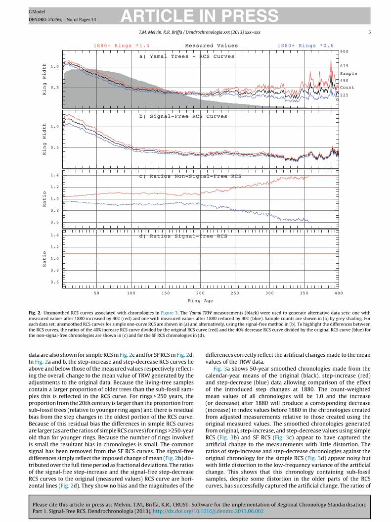
Fig. 2. Unsmoothed RCS curves associated with chronologies in Figure 3. The Yamal TRW measurements (black) were used to generate alternative data sets: one withmeasured values after 1880 increased by 40% (red) and one with measured values after 1880 reduced by 40% (blue). Sample counts are shown in (a) by grey shading. Foreach data set, unsmoothed RCS curves for simple one-curve RCS are shown in (a) and alternatively, using the signal-free method in (b). To highlight the differences betweent curvet n (d).

dIaiacppsbBaoisdtoRz

dv

caom((fofRaro

he RCS curves, the ratios of the 40% increase RCS curve divided by the original RCShe non-signal-free chronologies are shown in (c) and for the SF RCS chronologies i

ata are also shown for simple RCS in Fig. 2c and for SF RCS in Fig. 2d.n Fig. 2a and b, the step-increase and step-decrease RCS curves liebove and below those of the measured values respectively reflect-ng the overall change to the mean value of TRW generated by thedjustments to the original data. Because the living-tree samplesontain a larger proportion of older trees than the sub-fossil sam-les this is reflected in the RCS curve. For rings > 250 years, theroportion from the 20th century is larger than the proportion fromub-fossil trees (relative to younger ring ages) and there is residualias from the step changes in the oldest portion of the RCS curve.ecause of this residual bias the differences in simple RCS curvesre larger (as are the ratios of simple RCS curves) for rings >250-yearld than for younger rings. Because the number of rings involveds small the resultant bias in chronologies is small. The commonignal has been removed from the SF RCS curves. The signal-freeifferences simply reflect the imposed change of mean (Fig. 2b) dis-


ributed over the full time period as fractional deviations. The ratiosf the signal-free step-increase and the signal-free step-decreaseCS curves to the original (measured values) RCS curve are hori-ontal lines (Fig. 2d). They show no bias and the magnitudes of the

wcsc

(red) and the 40% decrease RCS curve divided by the original RCS curve (blue) for

ifferences correctly reflect the artificial changes made to the meanalues of the TRW data.

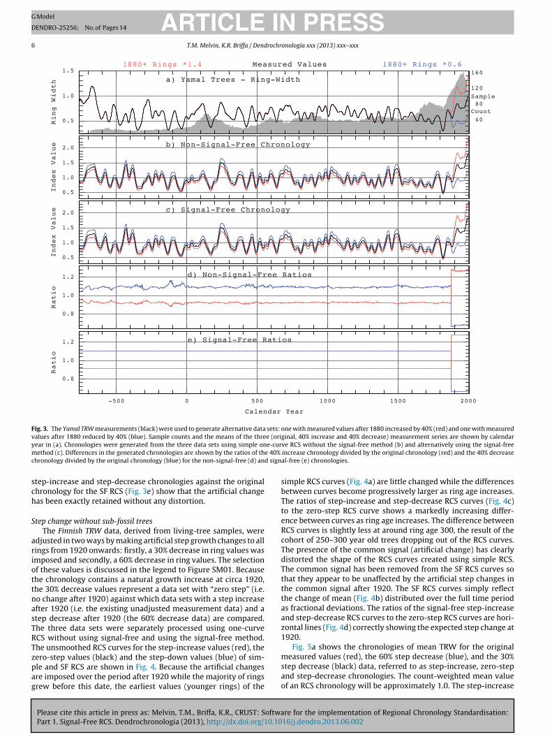
Fig. 3a shows 50-year smoothed chronologies made from thealendar-year means of the original (black), step-increase (red)nd step-decrease (blue) data allowing comparison of the effectf the introduced step changes at 1880. The count-weightedean values of all chronologies will be 1.0 and the increase

or decrease) after 1880 will produce a corresponding decreaseincrease) in index values before 1880 in the chronologies createdrom adjusted measurements relative to those created using theriginal measured values. The smoothed chronologies generatedrom original, step-increase, and step-decrease values using simpleCS (Fig. 3b) and SF RCS (Fig. 3c) appear to have captured thertificial change to the measurements with little distortion. Theatios of step-increase and step-decrease chronologies against theriginal chronology for the simple RCS (Fig. 3d) appear noisy but


ith little distortion to the low-frequency variance of the artificialhange. This shows that this chronology containing sub-fossilamples, despite some distortion in the older parts of the RCSurves, has successfully captured the artificial change. The ratios of





Sample

Count

160

120

80

400.5

1.0

1.5

Ring Width

1880+ Rings *0.61880+ Rings *1.4 Measured Values

a) Yamal Trees - Ring-Width

0.5

1.0

1.5

2.0

Index Value b) Non-Signal-Free Chronolog y

0.5

1.0

1.5

2.0

Index Value c) Signal-Free Chronology

0.8

1.0

1.2

Ratio

d) Non-Signal-Free Ratios

-500 0 500 1000 1500 2000

Calendar Year

0.8

1.0

1.2

Ratio

e) Signal-Free Ratios

Fig. 3. The Yamal TRW measurements (black) were used to generate alternative data sets: one with measured values after 1880 increased by 40% (red) and one with measuredvalues after 1880 reduced by 40% (blue). Sample counts and the means of the three (original, 40% increase and 40% decrease) measurement series are shown by calendary e-curm e 40%

c d sign

sch

S

ariottnasTRTzpag

sbTteRcTdTtttaaz1

ear in (a). Chronologies were generated from the three data sets using simple onethod (c). Differences in the generated chronologies are shown by the ratios of th

hronology divided by the original chronology (blue) for the non-signal-free (d) an

tep-increase and step-decrease chronologies against the originalhronology for the SF RCS (Fig. 3e) show that the artificial changeas been exactly retained without any distortion.

tep change without sub-fossil treesThe Finnish TRW data, derived from living-tree samples, were

djusted in two ways by making artificial step growth changes to allings from 1920 onwards: firstly, a 30% decrease in ring values wasmposed and secondly, a 60% decrease in ring values. The selectionf these values is discussed in the legend to Figure SM01. Becausehe chronology contains a natural growth increase at circa 1920,he 30% decrease values represent a data set with “zero step” (i.e.o change after 1920) against which data sets with a step increasefter 1920 (i.e. the existing unadjusted measurement data) and atep decrease after 1920 (the 60% decrease data) are compared.he three data sets were separately processed using one-curveCS without using signal-free and using the signal-free method.he unsmoothed RCS curves for the step-increase values (red), the


ero-step values (black) and the step-down values (blue) of sim-le and SF RCS are shown in Fig. 4. Because the artificial changesre imposed over the period after 1920 while the majority of ringsrew before this date, the earliest values (younger rings) of the

msao

ve RCS without the signal-free method (b) and alternatively using the signal-freeincrease chronology divided by the original chronology (red) and the 40% decreaseal-free (e) chronologies.

imple RCS curves (Fig. 4a) are little changed while the differencesetween curves become progressively larger as ring age increases.he ratios of step-increase and step-decrease RCS curves (Fig. 4c)o the zero-step RCS curve shows a markedly increasing differ-nce between curves as ring age increases. The difference betweenCS curves is slightly less at around ring age 300, the result of theohort of 250–300 year old trees dropping out of the RCS curves.he presence of the common signal (artificial change) has clearlyistorted the shape of the RCS curves created using simple RCS.he common signal has been removed from the SF RCS curves sohat they appear to be unaffected by the artificial step changes inhe common signal after 1920. The SF RCS curves simply reflecthe change of mean (Fig. 4b) distributed over the full time periods fractional deviations. The ratios of the signal-free step-increasend step-decrease RCS curves to the zero-step RCS curves are hori-ontal lines (Fig. 4d) correctly showing the expected step change at920.

Fig. 5a shows the chronologies of mean TRW for the original


easured values (red), the 60% step decrease (blue), and the 30%tep decrease (black) data, referred to as step-increase, zero-stepnd step-decrease chronologies. The count-weighted mean valuef an RCS chronology will be approximately 1.0. The step-increase





Sample

Count

100

75

50

25

0.5

1.0

Ring Width

1920+ Rings *0.4Measured Value s 1920+ Rings *0.7

a) Finnish Trees - RCS Curves

0.5

1.0

Ring Width

b) Signal-Free RCS Curves

0.6

0.8

1.0

1.2

1.4

Ratio

c) Ratios Non-Signal-Free RCS

50 100 150 200 250 300 350 400

Ring Age

0.6

0.8

1.0

1.2

1.4

Ratio

d) Ratios Signal-free RCS

Fig. 4. Unsmoothed RCS curves associated with chronologies from Fig. 5 created from Finnish TRW data. Sample counts (grey shading) are shown in (a). The means of TRWby ring age for the measured values (red), 30% decrease after 1920 chronology (black), and 60% decrease after 1920 chronology (blue) referred to as step-increase, zero-stepand step-decrease data are shown in (a) and (b). Unsmoothed RCS curves for one-curve RCS without using the signal-free method are shown in (a) and alternatively usingt s, thes RCS cu

(1ttscsebUftdcoifcTs

oumbz

C

tatltsTR

he signal-free method (b). To highlight the differences in the generated RCS curvehown in (red) and secondly the step-decrease RCS curve divided by the zero-step

step-decrease) chronology will have lower (higher) values before920 relative to the zero-step chronology. For simple RCS prioro 1920 (Fig. 5b), the slope of the step-increase chronology is lesshan the slope of the zero-step chronology and the slope of thetep-decrease chronology is greater than the slope of the zero-stephronology. The ratios of chronologies (Fig. 5d) of step-increase andtep-decrease divided by the zero-step chronology show that theffect of the artificial step changes is to produce a consistent slopeias in these non-signal-free chronologies over their full period.sing simple RCS the overall slope of a chronology without sub-

ossil trees is unpredictable. What has occurred is that the changeo the common signal at 1920 (step-increase or step-decrease) isistributed across the older section of the RCS curve because theonstituent tree ages vary considerably. This has changed the slopef the RCS curve and this change of slope produces the slope biasn the chronologies. The proportion of chronology slope generated


rom the changing mean values of tree index-series (caused byhanging common forcing over time) is captured by simple RCS.he proportion of chronology slope generated from the averagelope of series of tree indices (the average slope of common forcing

swsa

ratios of firstly the step-increase RCS curve divided by the zero-step RCS curve isrve is shown in (blue) for the non-signal free (c) and signal-free method (d).

ver the life of a tree) has been lost. The chronologies generatedsing SF RCS (Fig. 5c) have captured the artificial change to theeasurements with little distortion as is shown by the ratios of

oth step-increase and step-decrease chronologies against theero-step chronology for the SF RCS implementation (Fig. 5e).

hronology slope recovery using simulated treesIt is known that for RCS the existence of a tree-growth-forcing

rend over the length of the chronology can cause problems (Briffand Melvin, 2011). In this case, measurements from the “average”ree will contain the average chronology slope over the tree’sifetime. An RCS curve constructed from such trees will containhis slope and the division by RCS values when detrending eacheries will remove the slope (Briffa and Melvin, 2011, Figure 5.2).he effects of positive and negative growth-forcing slopes onCS curves and resulting chronologies are explored here using


imulated trees. Pseudo sub-fossil and living-tree chronologiesere generated from series of simulated TRW measurements. The

imulated chronology signals consisted of either a positive or neg-tive linear slope over the length of the chronology with a range





Sample

Count

100

75

50

25

0.5

1.0

Ring Width

1920+ Rings *0.4Measured Value s 1920+ Rings *0.7

a) Finnish Trees - Ring-Widt h

0.5

1.0

1.5

Index Value b) Non-Signal-Free Chronolog y

0.5

1.0

1.5


0.6

0.8

1.0

1.2

Ratio

d) Non-Signal-Free Ratios

1600 1650 1700 1750 1800 1850 1900 1950 2000

Calendar Year

0.6

0.8

1.0

1.2

Ratio

e) Signal-Free Ratios

Fig. 5. The Finnish TRW measurements (red) were used to generate alternative data sets: one with measured values after 1920 reduced by 30% (black) and one withmeasured values after 1920 reduced by 60% (blue). Sample counts and the mean of the three (original here containing a natural “step-increase”, 30% decrease “zero-step”,and 60% decrease “step-decrease”) measurement series are shown by calendar year in (a). Chronologies were generated from the three data sets with one-curve RCS withoutu . Diffei p-decrc

fvrotwRcfaoat2ctotteo

bRsimacuoat

C

nss

sing the signal-free method (b) and alternatively using the signal-free method (c)ncrease chronology divided by the zero-step chronology (red) and secondly, the stehronologies (d) and for the SF RCS chronologies (e).

rom 0.8 to 1.2. TRW measurements consist of the chronologyalues over the life of the tree multiplied by “white noise” with aange 0.95–1.05. All pseudo trees have start dates evenly-spacedver time. The pseudo-sub-fossil trees are all 200 years old andhe living trees all have the same final year. The four data setsere standardised using simple one-curve RCS and one-curve SFCS. The chronologies are shown in Fig. 7 and the associated RCSurves are shown in Fig. 6. The simple RCS chronologies derivedrom simulated sub-fossil trees, (Fig. 7a and b, blue lines), shown end-effect distortion. The average slope of the chronologyver the life of each tree appears in the RCS curve (Fig. 6a and b)nd is removed from each individual tree-series in detrending. Inhe central portions of the chronologies (between nominal years00 and 800) the chronology slope is correctly captured by thehanging mean values of tree-index series. The loss of slope ofrees (decrease at the start and increase at the end of each seriesf tree indices) in this section of the chronology does not change


he chronology because the beginning of one tree overlaps withhe end of another tree and these effects cancel. At the start (andnd) of the chronologies there are no second-halves (first halves)f trees to compensate and the loss of slope produces systematic

ayya

rences in the generated chronologies are shown by the ratios: firstly, of the step-ease chronology divided by the zero-step chronology (blue) for the non-signal-free

ias in the beginnings and ends of these chronologies. The simpleCS living-tree chronologies (Fig. 7c and d, blue curves) lose thelopes contained in the respective RCS curves (Fig. 6c and d) butn each case they do retain the slope related to the changing

ean values of each tree-index series. In this example the earlynd late end-effect biases effectively join in the middle of thehronology so that the living-tree chronology processed withoutsing the signal-free implementation suffers a serious partial lossf chronology slope. In the corresponding examples, where there is

wide distribution of tree ages, the signal-free method overcomeshis slope bias problem (Fig. 7c and d, red curves).

hronology slope change using living treesThe Finnish TRW measurements were adjusted to generate alter-

ative data sets: one with the chronology slope reduced (decreasedlope) and one with the chronology slope increased (increasedlope), where each measurement was multiplied by the appropri-


te factor for that year to rotate the chronology about the centreear of the chronology, with a change of slope of 0.001 mm perear. The unsmoothed RCS curves for the original, increased-slopend decreased-slope data with and without using the signal-free





Sample

Count

100

75

50

250.8

1.0

1.2

Ring Width

a) Sub-Fossil Negative Slope

Simple RCS Curve Signal-free RCS Curve

20 40 60 80 100 120 140 160 180 200

0.8

1.0

1.2

Ring Width

b) Sub-Fossil Positive Slope

Sample

Count

50

37

25

120.8

1.0

1.2

Ring Width

c) Living Tree Negative Slop e

50 100 150 200 250 300 350 400

Ring Age

0.8

1.0

1.2

Ring Width

d) Living Tree Positive Slop e

Fig. 6. Unsmoothed RCS curves associated with chronologies in Fig. 7. Sub-fossil and living chronologies were generated from series of simulated TRW measurements. Thesimulated chronology signals consisted of either a positive or negative linear slope over the length of the chronology. TRW measurements consist of the chronology valuesover the life of the tree with added random “noise”. The four data sets were standardised using simple one-curve RCS (blue) and one-curve SF RCS (red). In (a) and (b) theslope of the chronology over 1000 years appears identically in each 200-year long tree. This slope appears in the simple RCS curves but does not appear in the SF RCS curves.I se the( e RCS

r he RCS

mTRooctstm

tatcoiawo

aisoosSsscsits

L

n (c) and (d) the slope of the chronology over 400 years appears in each tree. Becaud) for the positive slope) than those of the oldest trees the RCS curves of the simplemoves the influence of the artificial signals added to these trees on the shape of t

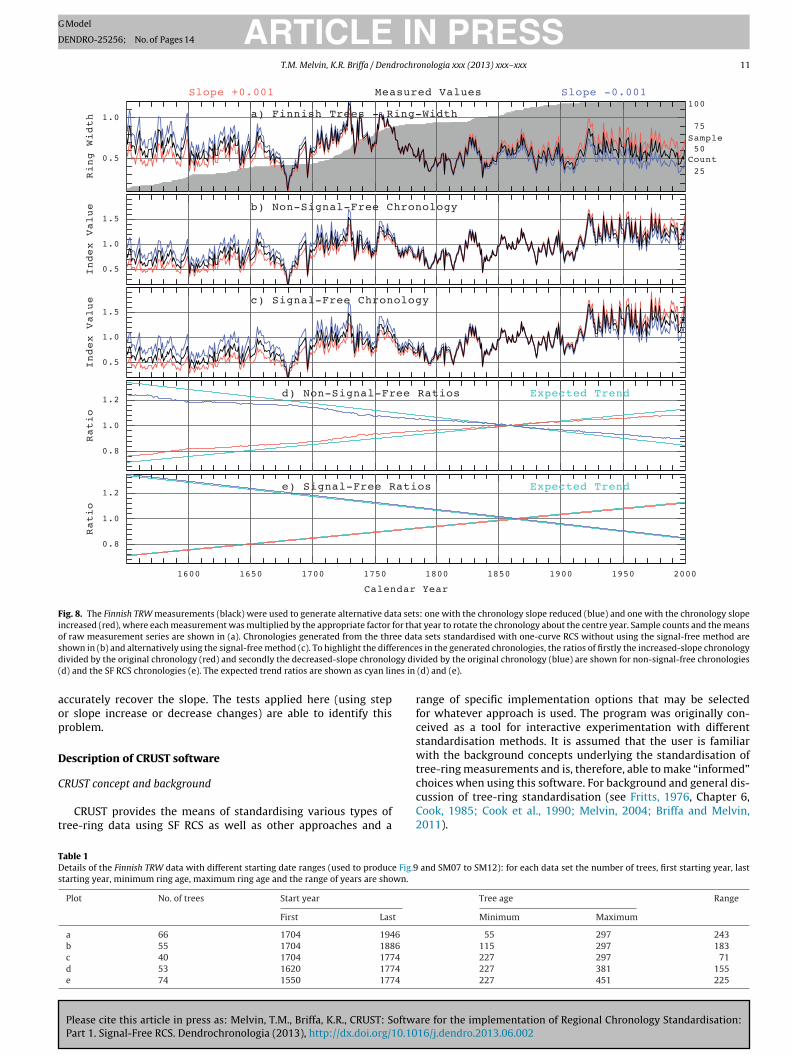
ethod are compared (see Figure SM02 and associated discussion).he simple RCS curves contain the slope changes whereas the SFCS curves are unbiased by the slope change. Chronologies for theriginal, increased-slope and decreased-slope data with and with-ut using the signal-free method are shown in Fig. 8. The simple RCShronology recovers the slope contained by the means of series ofree indices but loses the portion of slope contained in the slopes oferies of tree indices (Fig. 8d). The signal-free method recovers bothypes of slope and thus successfully recovers the artificial changes

ade to the original data (Fig. 8e).The slope of a living-tree RCS chronology comes from both

he changing mean values of series of tree indices over timend the mean of the slopes of series of tree indices. To evaluateheir separate contributions we explored the effects on living-treehronologies of changing the means of series of tree indices with-ut changing the slopes and changing the slopes of series of tree


ndices without changing the means. For this we used artificiallydjusted versions of the Finnish TRW data. Firstly, slope changesere applied to individual series of measurements but the mean

f each series was left unchanged (Figures SM03 and SM04 and

rdo

mean values of the younger trees are greater for the negative (c) slope (and lower(blue) are not straight lines but curve slightly. The signal-free method successfully

curves in all cases. Sample counts are shown by grey shading.

ssociated discussion). This demonstrates that the mean values ofndex series over time is an important contributor to chronologylope in a living-tree chronology and is necessary for the successfulperation of SF RCS. Secondly, the effect of changing the chronol-gy slope was applied to the mean TRW of individual measurementeries but the slopes of each series were left unchanged (FiguresM05 and SM06). This indicates that the slopes of measurementeries over time also make an important contribution to chronologylope in living-tree chronologies and are also necessary for the suc-essful operation of SF RCS. To recover the full chronology slope, theignal-free method requires that the two components of the slope.e. that contained in the mean values of index series and that con-ained in the slopes of those series, are present in the measurementeries.

iving trees with reduced time span


The requirement for large numbers of sub-fossil trees can beelaxed with the use of SF RCS provided rings of the same age areistributed over a wide time range. Incorporating a wider rangef tree starting years (i.e. a wide range of ring ages in living-tree





Sample

Count

50

37

25

120.8

1.0

1.2

Index Value

Expected Trend

a) Sub-Fossil Negative Slope

Simple RCS Chronology Signal-free RCS Chronology

100 200 300 400 500 600 700 800 900 1000

0.8

1.0

1.2

Index Value

b) Sub-Fossil Positive Slope

Sample

Count

50

37

25

12

1.0

1.2

1.4

Index Value

c) Living Tree Negative Slop e

50 100 150 200 250 300 350 400

Nominal Calendar Year

0.8

1.0

1.2

Index Value

d) Living Tree Positive Slop e

Fig. 7. Sub-fossil and living chronologies were generated from series of simulated TRW measurements consisting of either a positive or negative linear slope over the lengthof the chronology with added random “white noise”. The four data sets were standardised using simple one-curve RCS and one-curve SF RCS. In each case the expectedc SF RC( le cou

daoca(cetirtdoi

swssrR

(z61(arc(sasctatcf

hronology signal is plotted as a black line. The simple RCS chronologies (blue) andb) and those generated from simulated living trees are shown in (c) and (d). Samp

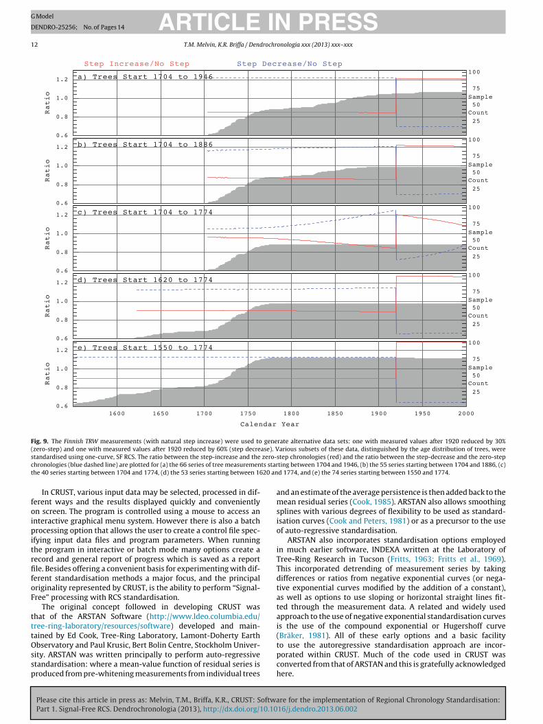
ata) produces a wider range of climate variability experiencedt each ring age and reduces the probability that climate fromne specific period will unduly influence the shape of the RCSurve. Here we consider how wide the time range must be tovoid distortion in chronologies. The three Finnish TRW data setsstep-increase, zero-step and step-decrease) as described in Stephange without sub-fossil trees are used. The trees in these data setsnd on the same year so the variation in start dates representshe spread over time of rings of the same ring-age. By systemat-cally removing trees, different data sets are created in which theange of start dates (and ages) of the remaining trees is reduced andhus each ring age of the RCS curve is represented by rings from aifferent restricted time range. Five data sets, (a) to (e), were devel-ped with different starting-date (and tree-age) ranges as shownn Table 1.

Detailed results are shown in Figures SM07 to SM11 for non-ignal-free and signal-free processing. These results show thatithout signal free, whatever the range of start dates for trees, the


imple RCS performs poorly with these adjusted-living-tree dataets and consistently creates chronologies whose slopes do noteflect the applied changes. Fig. 9 summarises the results for SFCS. The ratios of step decrease chronology to zero step chronology

esot

S chronologies (red) derived from simulated sub-fossil trees are shown in (a) andnts are shown by grey shading.

blue dashed lines) and the ratios of step increase chronology toero step chronology (red lines) are plotted using data from (a)6 trees with a 243-year range in starting years (from 1704 to946), (b) 55 trees with a 183-year range (from 1704 to 1882),c) 40 trees with a 71-year range (from 1704), (d) 53 trees with

155-year range (from 1620), and (e) 74 trees with a 225-yearange (from 1550). For (a) and (e) there is no distortion in theaptured signal, while for (b) and (d) there is slight distortion. Forc) there is considerable distortion in the recovered signals. As thetarting-year range is reduced below 200 years some distortionppears even when using the signal-free method and with atarting-year range of length less than 100 years distortion isonsiderable. Figure SM12 shows results similar to Fig. 9 excepthat the artificial adjustments in this case, instead of step changesre a slope increase and a slope decrease. This demonstrates thathe ability to capture slope changes is very similar to that for stephanges. With only 71 years variation in ring start dates the signal-ree method cannot recover the artificial changes correctly. In this


xample, simply including either 15 younger or 13 older treesubstantially corrects the problem and including either 26 youngerr 34 older trees completely corrects the problem. Provided thathere is a sufficiently wide distribution of tree ages, the SF RCS can





Sample

Count

100

75

50

25

0.5

1.0

Ring Width

Slope -0.001Slope +0.001 Measured Values

a) Finnish Trees - Ring-Width

0.5

1.0

1.5

Index Value b) Non-Signal-Free Chronology

0.5

1.0

1.5


0.8

1.0

1.2

Ratio

Expected Trendd) Non-Signal-Free Ratios

1600 1650 1700 1750 1800 1850 1900 1950 2000

Calendar Year

0.8

1.0

1.2

Ratio

Expected Trende) Signal-Free Ratios

Fig. 8. The Finnish TRW measurements (black) were used to generate alternative data sets: one with the chronology slope reduced (blue) and one with the chronology slopeincreased (red), where each measurement was multiplied by the appropriate factor for that year to rotate the chronology about the centre year. Sample counts and the meansof raw measurement series are shown in (a). Chronologies generated from the three data sets standardised with one-curve RCS without using the signal-free method ares renced gy div( es in

aop

D

C

t

rfcswt

TDs

hown in (b) and alternatively using the signal-free method (c). To highlight the diffeivided by the original chronology (red) and secondly the decreased-slope chronolod) and the SF RCS chronologies (e). The expected trend ratios are shown as cyan lin

ccurately recover the slope. The tests applied here (using stepr slope increase or decrease changes) are able to identify thisroblem.

escription of CRUST software


RUST concept and background

CRUST provides the means of standardising various types ofree-ring data using SF RCS as well as other approaches and a

ccC2

able 1etails of the Finnish TRW data with different starting date ranges (used to produce Fig.9

tarting year, minimum ring age, maximum ring age and the range of years are shown.

Plot No. of trees Start year

First Last

a 66 1704 1946

b 55 1704 1886

c 40 1704 1774

d 53 1620 1774

e 74 1550 1774

s in the generated chronologies, the ratios of firstly the increased-slope chronologyided by the original chronology (blue) are shown for non-signal-free chronologies

(d) and (e).

ange of specific implementation options that may be selectedor whatever approach is used. The program was originally con-eived as a tool for interactive experimentation with differenttandardisation methods. It is assumed that the user is familiarith the background concepts underlying the standardisation of

ree-ring measurements and is, therefore, able to make “informed”


hoices when using this software. For background and general dis-ussion of tree-ring standardisation (see Fritts, 1976, Chapter 6,ook, 1985; Cook et al., 1990; Melvin, 2004; Briffa and Melvin,011).

and SM07 to SM12): for each data set the number of trees, first starting year, last

Tree age Range

Minimum Maximum

55 297 243115 297 183227 297 71227 381 155227 451 225





Sample

Count

100

75

50

25

0.6

0.8

1.0

1.2

Ratio

Step Decrease/No StepStep Increase/No Step

a) Trees Start 1704 to 1946

Sample

Count

100

75

50

25

0.6

0.8

1.0

1.2

Ratio

b) Trees Start 1704 to 1886

Sample

Count

100

75

50

25

0.6

0.8

1.0

1.2

Ratio

c) Trees Start 1704 to 1774

Sample

Count

100

75

50

25

0.6

0.8

1.0

1.2

Ratio

d) Trees Start 1620 to 1774

Sample

Count

100

75

50

25

1600 1650 1700 1750 1800 1850 1900 1950 2000

Calendar Year

0.6

0.8

1.0

1.2

Ratio

e) Trees Start 1550 to 1774

Fig. 9. The Finnish TRW measurements (with natural step increase) were used to generate alternative data sets: one with measured values after 1920 reduced by 30%(zero-step) and one with measured values after 1920 reduced by 60% (step decrease). Various subsets of these data, distinguished by the age distribution of trees, weres zero-c ts start 20 an

foipitrfifoF

tttOssp

amsio

iTTdtatai(

tandardised using one-curve, SF RCS. The ratio between the step-increase and thehronologies (blue dashed line) are plotted for (a) the 66 series of tree measuremenhe 40 series starting between 1704 and 1774, (d) the 53 series starting between 16

In CRUST, various input data may be selected, processed in dif-erent ways and the results displayed quickly and convenientlyn screen. The program is controlled using a mouse to access annteractive graphical menu system. However there is also a batchrocessing option that allows the user to create a control file spec-

fying input data files and program parameters. When runninghe program in interactive or batch mode many options create aecord and general report of progress which is saved as a reportle. Besides offering a convenient basis for experimenting with dif-

erent standardisation methods a major focus, and the principalriginality represented by CRUST, is the ability to perform “Signal-ree” processing with RCS standardisation.

The original concept followed in developing CRUST washat of the ARSTAN Software (http://www.ldeo.columbia.edu/ree-ring-laboratory/resources/software) developed and main-ained by Ed Cook, Tree-Ring Laboratory, Lamont-Doherty Earth


bservatory and Paul Krusic, Bert Bolin Centre, Stockholm Univer-ity. ARSTAN was written principally to perform auto-regressivetandardisation: where a mean-value function of residual series isroduced from pre-whitening measurements from individual trees

tpch

step chronologies (red) and the ratio between the step-decrease and the zero-stepting between 1704 and 1946, (b) the 55 series starting between 1704 and 1886, (c)d 1774, and (e) the 74 series starting between 1550 and 1774.

nd an estimate of the average persistence is then added back to theean residual series (Cook, 1985). ARSTAN also allows smoothing

plines with various degrees of flexibility to be used as standard-sation curves (Cook and Peters, 1981) or as a precursor to the usef auto-regressive standardisation.

ARSTAN also incorporates standardisation options employedn much earlier software, INDEXA written at the Laboratory ofree-Ring Research in Tucson (Fritts, 1963; Fritts et al., 1969).his incorporated detrending of measurement series by takingifferences or ratios from negative exponential curves (or nega-ive exponential curves modified by the addition of a constant),s well as options to use sloping or horizontal straight lines fit-ed through the measurement data. A related and widely usedpproach to the use of negative exponential standardisation curvess the use of the compound exponential or Hugershoff curveBräker, 1981). All of these early options and a basic facility


o use the autoregressive standardisation approach are incor-orated within CRUST. Much of the code used in CRUST wasonverted from that of ARSTAN and this is gratefully acknowledgedere.


http://www.ldeo.columbia.edu/tree-ring-laboratory/resources/software

http://www.ldeo.columbia.edu/tree-ring-laboratory/resources/software

ING Model

D

rochr

wttcamu

P

wca

melv

p

uss

c

r

bs

o

R

ud

i

as

ic

i

Sc

C

RCfooti

slottrrsawctoDq

lcesHomctb

eiowRsupi

oTdotco

A

(HPsi

A

i0



A very basic outline of the major processing options availableithin CRUST is provided below. This is included here only to illus-

rate the scope of the software. More details are to be found inhe “CRUST: Program Documentation” available at http://www.ru.uea.ac.uk/cru/papers/melvin2013dendrochronologia/. There islso some online help provided when CRUST is used in interactiveode, through a number of drop-down dialogue boxes accessed

sing the right button of the mouse.

rincipal CRUST standardisation options

The following is a list of the major options available for selectionithin CRUST. The expressions in parentheses identify the specific

ontrol parameters used within CRUST. A number of these optionsre from those available within other standardisation software.

Detrending Method (IDT) select from: RCS method; no detrend;odified negative exponential or any slope line; modified negative

xponential or a negative slope line; any slope line; negative slopeine; horizontal line; Hugershoff curve; general exponential; andarious smoothing splines.

Transform options (ITN) select from: no transform; adaptiveower transform; or basal area transform.

RCS curve smoothing (RDT) select from: age dependant spline;nsmoothed RCS curve; modified negative exponential; fittedtraight line; Hugershoff curve; spline with selected stiffness; orpline with % length stiffness.

Index Creation options (IND) select from: ratios or residuals toreate tree index series.

Index Averaging options (KRB) select from: arithmetic mean orobust mean.

Variance Stabilisation options (ISB) select from: no variance sta-ilisation; variance stabilisation; or high-frequency-only variancetabilisation.

Signal-Free (SFO) select from: signal-free or not signal-free.Pith-Offset Estimates (POO) select from; use pith offset estimates

r do not use pith offset estimates.Single RCS Curve (SRC) select from: single RCS curve; multiple-

CS curves; or the use of pre-specified RCS curves.Type of RCS curve (TRC) select from: use age-based RCS curves;

se diameter-based RCS curves; or use the average of age- andiameter-based RCS curves.

RCS Transform options (GTR) select from: use un-transformedndices or indices transformed by mean growth rate.

Tree Sorting options (TST) select from: do not sort; sort by treege; sort by tree diameter; sort by growth rate; sort by tree name;ort by pith year; or sort by final year.

Chronology Mean options (BFC) select from: mean of all treendices; or arithmetic mean of chronologies; or the mean withhronology means set to 1.0.

Normal Distribution option (BFC) select from: use untransformedndices; or convert tree index distribution to normal.

Autoregressive Modelling options (BFC) select from: create theTD chronology; create the ARS chronology; or create the REShronology.

onclusions

We have reviewed the basic concepts of simple and signal-freeCS and described the implementation options available withinRUST. We have demonstrated superior performance of the signal-

ree approach in a number of examples selected to test the ability


f RCS to recover known growth-forcing signals. The overall slopef living-tree chronologies generated using simple RCS is uncer-ain because the chronology slope appears in the RCS curve ands largely removed from the chronology by division. This problem

R

B

PRESSonologia xxx (2013) xxx– xxx 13

everely limits the value of the simple RCS method for processingiving-tree chronologies. As previously described, the availabilityf large numbers of sub-fossil trees spanning a period much longerhan the length of individual trees will, in general, greatly reducehis problem so that it becomes only an “end effect” bias often ofelatively small magnitude. The signal-free method reduces theequirement for a large temporal distribution of trees (i.e. manyub-fossil trees) and mitigates the “end-effect” bias. RCS is unsuit-ble for processing the data from a near equal-aged cohort of treeshose growth terminates at the same time. A sample living-tree

hronology processed using the signal-free method showed no dis-ortion in the recovery of imposed signal changes where the rangef tree ages spanned at least half the length of the chronology.istortion was significant when the age range was less than oneuarter the length of the chronology.

By artificially adjusting chronologies it is possible to test theikely presence of bias in the slope of those chronologies. If appliedhanges representing known growth-forcing signals can be recov-red without serious distortion it is reasonable to assume that theignal recovered from the original chronology is also undistorted.owever, if the known signals are distorted then it may be that theriginal chronology is distorted. Only a limited extent of experi-entation with the SF approach has been done to date and there is

onsiderable scope for further work in other contexts. However, onhe basis of results to date we conclude that Signal-Free RCS shoulde used as the standard method of RCS processing.

The signal-free approach clearly improves the performance andxtends the situations in which RCS can be used. However, it ismportant to stress that its value lies in its ability to mitigate onlyne source of potential bias: the distortion in RCS curves associatedith residual common-signal variance. As with simple RCS the SFCS cannot overcome chronology bias caused by inhomogeneousamples, particularly the “modern sample bias” associated with thenintentional selection of recent, relatively fast-growing tree sam-les that are inconsistent compared with sample composition back

n time (Briffa and Melvin, 2011).In Part 2 of this paper we discuss the justification and make rec-

mmendations for the use of other CRUST implementation options.hese include: the use of pith offset data; using ratios rather thanifferences in calculating chronology indices; the transformationf tree indices so that they have a normal distribution; an alterna-ive calculation of EPS with a focus on low-frequency chronologyonfidence and the use of multiple rather than single RCS curves tovercome modern sample bias.

cknowledgements

TMM and KRB acknowledge support from UK NERCNE/G018863/1). We are grateful to Hakan Grudd and Rashitantemirov for the provision of tree-ring data and to Ed Cook,aul Krusic and Kurt Nicolussi for continuing discussions abouttandardisation concepts in general and detailed aspects of CRUSTmplementation.

ppendix A. Supplementary data

Supplementary data associated with this article can be found,n the online version, at http://dx.doi.org/10.1016/j.dendro.2013.6.002.


eferences

räker, O.U., 1981. Der Alterstrend bei Jahrringdichten und Jahrringbreiten vonNadelhölzern und sein Ausgleich. Mitteilungen der Forstlichen Bundesversuch-sanstalt Wien 142, 75–102.


http://www.cru.uea.ac.uk/cru/papers/melvin2013dendrochronologia/

http://www.cru.uea.ac.uk/cru/papers/melvin2013dendrochronologia/

http://dx.doi.org/10.1016/j.dendro.2013.06.002

http://dx.doi.org/10.1016/j.dendro.2013.06.002

http://refhub.elsevier.com/S1125-7865(13)00047-7/sbref0005





















ING Model

D

1 rochr

B

B

B

B

C

C

C

C

E

E

F

FF

G

H

H

M

M

Melvin, T.M., Briffa, K.R., Nicolussi, K., Grabner, M., 2007. Time-varying-responsesmoothing. Dendrochronologia 25, 65–69.


4 T.M. Melvin, K.R. Briffa / Dend

riffa, K.R., Jones, P.D., Bartholin, T.S., Eckstein, D., Schweingruber, F.H., Karlén, W.,Zetterberg, P., Eronen, M., 1992. Fennoscandian Summers from AD 500: tem-perature changes on short and long timescales. Climate Dynamics 7, 111–119.

riffa, K.R., Jones, P.D., Schweingruber, F.H., Karlén, W., Shiyatov, S.G., 1996. Tree-ring variables as proxy-climate indicators: problems with low frequency signals.In: Jones, P.D., Bradley, R.S., Jouzel, J. (Eds.), Climatic Variations and ForcingMechanisms of the Last 2000 Years. Springer-Verlag, Berlin, pp. 9–41.

riffa, K.R., Melvin, T.M., 2011. A closer look at Regional Curve Standardisationof tree-ring records: justification of the need, a warning of some pitfalls, andsuggested improvements in its application. In: Hughes, M.K., Diaz, H.F., Swet-nam, T.W. (Eds.), Dendroclimatology: Progress and Prospects. Springer Verlag,Dordrecht, pp. 113–145.

riffa, K.R., Melvin, T.M., et al., 2013. Reassessing the evidence for tree-growth andinferred temperature change during the Common Era in Yamalia, northwestSiberia. Quaternary Science Reviews 72, 83–107.

ook, E.R., 1985. A Time-Series Analysis Approach to Tree-Ring Standardisation.University of Arizona, Tucson.

ook, E.R., Briffa, K.R., Meko, D.M., Graybill, D.A., Funkhouser, G., 1995. The segmentlength curse in long tree-ring chronology development for paleoclimatic studies.Holocene 5, 229–237.

ook, E.R., Briffa, K.R., Shiyatov, S., Mazepa, V., 1990. Tree-ring standardisation andgrowth trend estimation. In: Cook, E.R., Kairiukstis, L.A. (Eds.), Methods of Den-drochronology. Kluwer Academic Publishers, Dordrecht, pp. 104–123.


ook, E.R., Peters, K., 1981. The smoothing spline: a new approach to standardiz-ing forest interior tree-ring width series for dendroclimatic studies. Tree-RingBulletin 41, 45–53.

rlandsson, S., 1936. Dendrochronological Studies. University of Upsala, Upsala,Sweden.

M

PRESSonologia xxx (2013) xxx– xxx

sper, J., Cook, E.R., Schweingruber, F.H., 2002. Low-frequency signals in long tree-ring chronologies for reconstructing past temperature variability. Science 295,2250–2253.

ritts, H.C., 1963. Computer programs for tree-ring research. Tree-Ring Bulletin 25,2–7.

ritts, H.C., 1976. Tree Rings and Climate. Academic Press, London, pp. 246–311.ritts, H.C., Mosimann, J.E., Bottorff, C.P., 1969. A revised computer program for

standardising tree-ring series. Tree-Ring Bulletin 29, 15–20.rudd, H., Briffa, K.R., Karlén, W., Bartholin, T.S., Jones, P.D., Kromer, B., 2002.

A 7400-year tree-ring chronology in northern Swedish Lapland: natural cli-matic variability expressed on annual to millennial timescales. Holocene 12,9657–665.

antemirov, R.M., Shiyatov, S.G., 2002. A continuous multimillennial ring-widthchronology in Yamal, northwestern Siberia. Holocene 12, 717–726.

untington, E., 1914. The Climate Factor as Illustrated in Arid America, Pub. No. 192.Carnegie Institute, Washington.

elvin, T.M., 2004. Historical Growth Rates and Changing Climatic Sen-sitivity of Boreal Conifers. University of East Anglia, Norwich (Thesis)http://www.cru.uea.ac.uk/cru/pubs/thesis/2004-melvin/

elvin, T.M., Briffa, K.R., 2008. A “Signal-Free” approach to dendroclimatic stan-dardisation. Dendrochronologia 26, 71–86.


elvin, T.M., Grudd, H., Briffa, K.R., 2012. Potential bias in “updating” tree-ringchronologies using Regional Curve Standardisation: re-processing 1500-yearsof Torneträsk density and ring-width data. Holocene 23, 364–373.























































































































































































































































































































http://www.cru.uea.ac.uk/cru/pubs/thesis/2004-melvin/











































article in press - climatic research unit - university of east anglia

Documents