article in press - materials technology · set-point variation in learning schemes with...
TRANSCRIPT

ARTICLE IN PRESS
Control Engineering Practice 17 (2009) 345–356
Contents lists available at ScienceDirect
Control Engineering Practice
0967-06
doi:10.1
� Corr
and Con
MD Ein
E-m
(M.F. He
journal homepage: www.elsevier.com/locate/conengprac
Set-point variation in learning schemes with applications to wafer scanners
Marcel F. Heertjes a,b,�, Rene M.J.G. van de Molengraft a
a Department of Mechanical Engineering, Dynamics and Control Technology, Eindhoven University of Technology, Den Dolech 2, 5600 MD Eindhoven, The Netherlandsb ASML, Mechatronic Systems Development, De Run 6501, 5504 DR Veldhoven, The Netherlands
a r t i c l e i n f o
Article history:
Received 17 November 2007
Accepted 18 August 2008Available online 5 November 2008
Keywords:
Finite impulse response modeling
Multi-input multi-output feed-forward
design
Motion control systems
(Nonlinear) Iterative learning control
Wafer scanners
61/$ - see front matter & 2008 Elsevier Ltd. A
016/j.conengprac.2008.08.004
esponding author at: Department of Mecha
trol Technology, Eindhoven University of Tec
dhoven, The Netherlands. Tel.: +3140 27 3342
ail addresses: [email protected], marcel.heer
ertjes), [email protected] (R.M.J.G.
a b s t r a c t
This paper presents a finite impulse response strategy to deal with set-point variation in learning
schemes. On the basis of converged learning forces obtained with learning control at a specific
acceleration set-point profile, a finite impulse response mapping is derived to generalize the learned
forces at a specific set-point toward arbitrary set-point profiles, thus relaxing the need for further
learning. The above strategy is applied to the motion control systems of a wafer scanner in a multi-input
multi-output feed-forward setting, where a variety of set-point profiles is used. Industrial potential is
demonstrated via robustness to set-point variation and the improvements obtained in settling-time
reduction.
& 2008 Elsevier Ltd. All rights reserved.
1. Introduction
In high-speed motion systems such as the reticle and the waferstages of a wafer scanner (Van de Wal, Van Baars, Sperling, &Bosgra, 2002) learning can significantly improve upon perfor-mance. This is because of the repetitive nature of its scanningmotion (Dijkstra & Bosgra, 2002; Rotariu, Ellenbroek, & Steinbuch,2003; Rotariu, Dijkstra, & Steinbuch, 2004). In learning, informa-tion of previous executions of a repeated motion is used to updatea command (usually a force) needed to counteract the effect ofsuch motion at future executions, see for example Bristow,Tharayil, and Alleyne (2006), Cai, Freeman, Lewin, and Rogers(2008), and Moore (1999) for learning algorithms and Gunnarssonand Norrlof (2001) and Tousain and Van der Meche (2001) forlearning designs. Variation in the scanning motion, however,avoids the application of the resulting commands learned at aspecific motion to be effective in achieving performance whenapplied during a different motion; see also Xu (1998), Xu and Tan(2002), Dixon and Chen (2003), Xu and Tan (2003), and Rotariu,Ellenbroek, Van Baars, and Steinbuch (2003) for a related problemstatement. For this purpose a finite impulse response mapping isused as proposed by Potsaid and Wen (2004). The forces learnedfor a representative acceleration set-point are mapped onto afinite impulse response (FIR) model. In the wafer scanningexample, this is done prior to the process of wafer illumination
ll rights reserved.
nical Engineering, Dynamics
hnology, Den Dolech 2, 5600
4; fax: +3140 27 33201.
van de Molengraft).
whereas during this process the learned forces are replaced bygeneralized learned forces being the result of the finite impulseresponse model and the acceleration set-points at hand; this isdifferent from a run-to-run control approach such as for exampleconsidered by Bode, Ko, and Edgar (2004) which lacks in situperformance measurement (the wafer needs to be furtherprocessed) and in which all set-points are known. In a generalmulti-input multi-output feed-forward setting, the advantages aretwofold. On one hand, learning during the process of waferscanning is avoided. This maintains the high standard ofperformance in terms of wafer throughput. On the other hand,learning is based on a small sub-set of a generally large variationof wafer set-points. This constitutes the efficiency of the method.
This paper has three contributions: (i) a generalized learningthrough FIR modeling for motion systems, (ii) a multi-input multi-output learning approach in case these motion systems areweakly coupled, and (iii) an application of learning in the fieldof industrial wafer scanners. The paper is further organized asfollows. In Section 2, the wafer scanner application, which servesas an experimental benchmark, is discussed in terms of itsrelevant motion control sub-systems, in particular, the reticle andwafer stage. Section 3 considers learning in the repetitive contextof scanning motion. Section 4 deals with FIR modeling for multi-input multi-output feed-forward design. A performance assess-ment using examples from an industrial wafer stage is presentedin Section 5. Section 6 summarizes the main findings of the paper.
2. Dynamics and control of wafer scanners
During the lithographic manufacturing of integrated circuits(ICs) wafer scanners achieve performance by combining nano-

ARTICLE IN PRESS
M.F. Heertjes, R.M.J.G. van de Molengraft / Control Engineering Practice 17 (2009) 345–356346
scale resolution with optimized wafer throughput. The waferscanning process, see for example Groot-Wassink, Van de Wal,Scherer, and Bosgra (2005) and Heertjes and Van de Wouw(2006), can be described as follows. Light from a laser passes froma reticle which contains an image, through a lens, which scalesdown the image, onto a wafer, see Fig. 1. Both reticle and wafer arepart of two separate sub-systems: the reticle stage and the waferstage. Each stage employs a dual stroke principle: a long stroke forlarge-range motion and a short stroke for accurate positioning.The short-stroke modules can be modeled as floating masseswhich are controlled in six degrees-of-freedom on a single-inputsingle-output basis. A distinction is made between scanningdirections and non-scanning directions. The scanning directions,for example the x- and y-directions of the short-stroke waferstage, are controlled on the basis of both feedback and feed-forward. The non-scanning directions, for example the x- andz-direction of the short-stroke reticle stage, are mainly controlledby feedback.
Each of the controlled short-stroke directions can be repre-sented by the simplified block diagram representation of Fig. 2which can be considered in the more general context of motioncontrol systems. On the basis of an acceleration set-point a andresulting command r, a servo error signal e is constructed via e ¼
r � y with y the actual position (or angle depending on the choiceof axis) of the considered plant P, in this case a short-stroke stage.The error signal e is fed into a feedback controller Cfb that aims atdisturbance rejection mainly induced by force disturbances f. Toobtain sufficient tracking accuracy, an SISO (and model-based)feed-forward controller Cff is added.
4.5m
2.5m
reticle stage
wafer stage
lens
Fig. 1. Wafer scanner representation and its main components.
a 1
s2
rCfb (s)
Cff (s)
+ e
-
Fig. 2. Simplified block diagram represe
The short-stroke (electro-)mechanics of both the reticle- andwafer stages in the individual directions are characterized bydouble integrator behavior along with the expression of higher-order dynamics. In controlling such dynamics, the feedbackcontroller Cfb is chosen as a series connection of three filterblocks: a proportional-integrator-derivative (PID) filter, whichaims at both disturbance rejection and robust stability, a second-order low-pass filter to avoid high-frequency noise amplification,and several notch filters to deal with resonant behavior in theplant. In the frequency-domain, the controlled electro-mechanicsare characterized by the open-loop frequency response functionOlðjoÞ ¼ CfbðjoÞPðjoÞ such as depicted in Fig. 3 for the scanningy-direction of both a reticle and a wafer stage. In Boderepresentation, this figure shows the characteristics derived froma closed-loop measurement (solid) along with the characteristicsof a model (dashed). From this figure, it is concluded that robuststability is sufficiently guaranteed.
The reticle and wafer stage can be considered in the simplifiedMIMO context of Fig. 4. Different from Fig. 2, interaction betweenthe feedback loops is modeled using cross-talk forces acting onthe considered plants: f xy acting on Pyy and f yx acting on Pxx.From stability point of view, these MIMO forces remain smallenough to justify the SISO feedback/feed-forward design approachrelated to Fig. 2. From performance standpoint, this is not the case.Given the tight performance specifications this industry is facedwith, it suffices to state that a zero settling control aim is notpossible without at least including some MIMO characteristics inthe feed-forward design. This is the purpose of the proposedlearning such as presented in the next sections. Herein the data-based MIMO feed-forward contributions are used atop the model-based SISO feed-forwards. The SISO feed-forwards, which strictlyspeaking become redundant, are kept as an initial estimate inachieving performance.
3. Iterative learning control
For controlled processes exhibiting repeated motion, iterativelearning control provides a means to learn updated commands(or forces) from past servo information and apply these com-mands at future executions (or trials) of such motion, see alsoChen and Hwang (2005), Mishra, Coaplen, and Tomizuka (2007),and Tayebi and Islam (2006). The latter with the aim to improveupon servo performance.
The MIMO context in which iterative learning control isapplied to the short-stroke stages of a wafer scanner is expressedby the simplified block diagram representation of Fig. 5. Differentfrom Fig. 4, each axis contains a set of learning controllers Cilc 2
fCilc;xx;Cilc;xy;Cilc;yx;Cilc;yyg used to counteract the recurring errorcontributions ex and ey induced by the acceleration set-pointprofiles ax and ay. For example, the x-axis contains a learningcontroller Cilc;xx which generates a force f ilc;xx. This force is used tocounteract the recurring part of the error response ex which isinduced by the acceleration set-point ax; note that this is the error
fff f
P (s)y+
+
ntation of a motion control system.

ARTICLE IN PRESS
101 102 103 104−80
0
50
101 102−180
0
180
ampl
itude
in d
Bph
ase
in d
egre
esrs modelledws modelledrs measuredws measured
f in Hz
103 104
Fig. 3. Bode representation of the measured open-loop frequency response functions of the short-stroke wafer (ws) and reticle (rs) stage dynamics in scanning direction
along with the characteristics of two double integrator-based models.
1s2
ax rx ex
fff, xx
Cfb, xx
Cff, xx
Pxxyx
fxy
1
s2
ay ry ey
fff, yy
Cfb, yy
Cff, yy
Pyyyy
fyx
+
+ +
++
+
Fig. 4. Simplified block diagram representation of the MIMO controller structure
such as encountered for both the short-stroke wafer and reticle stages.
1
s2
ax rx ex
filc, yx
filc, xx
fff, xx
Cfb, xx
Cff, xx
Cilc, yx
Cilc, xx
Pxxyx
fxy
1
s2
ay ry ey
filc, xy
filc, yy
fff, yy
Cfb, yy
Cff, yy
Cilc, xy
Cilc, yy
Pyy
yy
fyx
+
+
+
+
+
++
+ ++
++
++
Fig. 5. Simplified block diagram representation of a simplified linear feedback
connection of two coupled short-stroke axes having iterative learning control.
M.F. Heertjes, R.M.J.G. van de Molengraft / Control Engineering Practice 17 (2009) 345–356 347
response after application of the SISO model-based feed-forwardcontroller Cff ;xx. Additionally—but applied in the y-axis—Cilc;xy
generates a force f ilc;xy used to counteract the recurring errorresponse ey. The latter being the result of cross-talk induced bythe set-point ax. The effectiveness of such a coupled systemcompensation stems from the assumption that the coupling issmall enough to endanger SISO stability but large enough toimprove upon MIMO performance. Hence the wafer stage plant ofabout 22.5 kg, which is accelerated in the y-direction with27:5 m s�2, requires feed-forward forces near Cff ;yy � 620 N. Sincef ilc;yy and f ilc;yx are typically in the order of 1 N, see Heertjes andTso (2007a), a sufficiently small coupling validates an essentiallySISO-based stability approach. However given a typical controllergain of 2� 107 N m�1 such learning forces correspond to errors inthe order of 50 nm which are large enough to allow for asignificant MIMO performance enhancement.
The learned forces f ilc in Fig. 5 comply with the schematicsof Fig. 6; see Heertjes and Tso (2007a) for a detailed SISO
description. That is, the error signals e related to a single executionof the acceleration set-point are stored in a buffer to formthe error column eðkÞ where k 2 N refers to the k-th execution(or trial). The buffer output is subjected to the nonlinear

ARTICLE IN PRESS
M.F. Heertjes, R.M.J.G. van de Molengraft / Control Engineering Practice 17 (2009) 345–356348
weighting U, or
UðeðkÞÞ ¼ diagðfðeðkÞf1gÞ;fðeðkÞf2gÞ; . . . ;fðeðkÞfngÞÞX0, (1)
with
fðxÞ ¼1�
djxj
if jxj4d;
0 if jxjpd:
8><>:
(2)
All entries in eðkÞ that are bounded in absolute value by athreshold level dX0 are assumed to be noise contributions and assuch are excluded from learning; typically d is chosen equal to theL1-norm of the steady-state signals obtained after all transientshave sufficiently damped out. Though limited in fully capturingthe noise characteristics, the choice for d along with the structureof (2) stems from both (nonlinear) stability and performanceconsiderations such as given in Heertjes and Tso (2007a, 2007b).After this weighting, the error signals are subjected to a linearlearning gain L which is given by
L ¼ ðSTpSp þ lIÞ�1ST
p, (3)
with tuning parameter l40, see Ghosh and Paden (2002).Basically, l is given the smallest possible value for which thelearning process is stable, such that L closely resembles the
Φ (·) L z−1 I
e
e (k) filc (k)
filc
filc (k+1)
Cilcbuffer
++
buffer
Fig. 6. Block diagram representation of the iterative learning control.
0 0.05−40
0
40
0 0.05−15
−303
15
18.2482 250010-1
100
101
t in s
e y in
nm
E y in
nm
cpsd
of E y
in n
m
f in Hz
Fig. 7. Time-series measurement of the error signals in y- and z-directions of a short str
20 different scans.
inverse process sensitivity S�1p and a fast convergence is obtained.
Sp 2 Rncon�nobs is given by
Sp ¼
h1 0 � � � 0
h2 h1 � � � 0
..
. ... . .
. ...
hncon hncon�1 . . . hncon�nobsþ1
2666664
3777775
, (4)
where ncon 2 N is the number of samples accessible for thelearning force, the so-called controller window and nobs 2 N isthe number of samples used for error evaluation, named theobservation window (Dijkstra & Bosgra, 2002). Sp has a Toeplitzstructure where h1;h2; . . . ;hn represent the Markov parameters. h1
represents the first error response sample e to a unitary forceimpulse f. The Markov parameters are obtained from measure-ment and typically reflect the average of 25 subsequent impulseresponse measurements as to reduce the effect of measurementnoise, see also Ahn, Moore, and Chen (2006) and Moore, Chen, andBahl (2005) for dealing with model uncertainty in this regard. Thelearning filters Cilc;xx and Cilc;yx (see Fig. 5) are both based on Sp;xx,hence they relate to the error response ex induced by a unitaryforce impulse f x. With Sp, the updated learned forces f ilcðkþ 1Þ aregiven by
filcðkþ 1Þ ¼ f ilcðkÞ þ LUðeðkÞÞeðkÞ, (5)
where f ilcðkÞ after buffering (see Fig. 6) gives the learned forces f ilc .For a detailed treatment of the stability and convergence proper-ties of such a nonlinear learning controller, the reader is referredto Heertjes and Tso (2007a, 2007b).
For a short-stroke reticle stage module, the need for MIMOlearning in view of (settling) performance is illustrated in Fig. 7.Given a representative acceleration profile ay, which—in scaledform—is depicted in the upper left part of the figure (dashedcurve), the servo error signals in y- and z-directions showsignificant response to the variation included in this profile. Notethat this is the response encountered under SISO model-based
0 0.05−400
0
400
0 0.05−200
−300
30
200
18.2482 2500100
101
102
t in s
f in Hz
e z in
nm
E z in
nm
cpsd
of E z
in n
m
oke reticle stage (upper part) along with the non-recurring residuals (lower part) of
ARTICLE IN PRESS
−0.2 −0.15 −0.1 −0.05 0 0.05 0.1 0.15 0.2−0.2
−0.15
−0.1
−0.05
0
0.05
0.1
0.15
0.2wafer stage top view
300 mm wafer
wafer scanning path
x-position in mm
y-po
sitio
n in
mm
Fig. 9. Graphical representation of a wafer scanning path during a job.
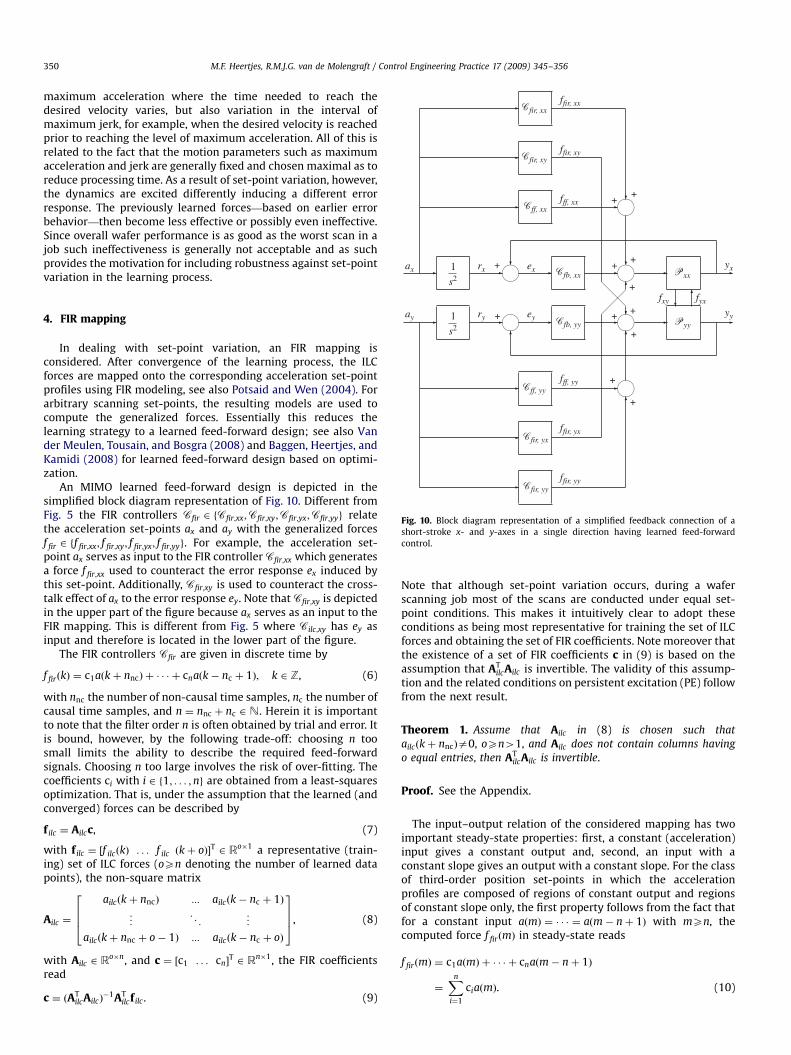
M.F. Heertjes, R.M.J.G. van de Molengraft / Control Engineering Practice 17 (2009) 345–356 349
feed-forward conditions. In the interval where performanceis required, i.e., the scanning interval of constant velocity, theresponses ey and ez induce an undesired settling time needed forthe error to become sufficiently small. The reproducibility of thesettling phenomenon is shown in the lower part of the figure.By comparing 20 separately measured error traces obtained insubsequent trials it can be seen that during constant velocity(beyond t ¼ 0:35 s) the residual errors E roughly remain inside anoise bound of �3 nm for the y-axis (left part) and �30 nm for thez-axis (right part); E is defined as Efig ¼ efig �
Pni¼1efig=n, with
n ¼ 20 and i referring to an error trace realization. A similarobservation follows for the root-mean-square values such asobtained via cumulative power spectral density (cpsd) analysis,which is shown in the lower part of the figure.
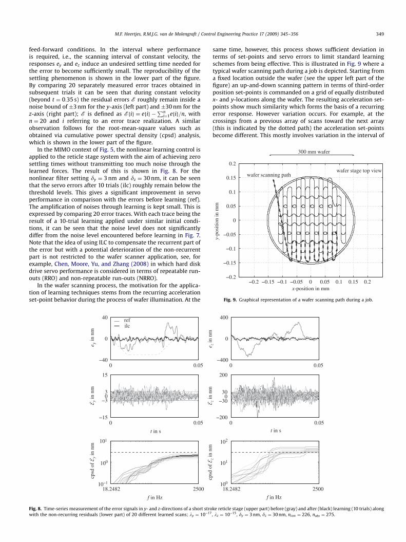
In the MIMO context of Fig. 5, the nonlinear learning control isapplied to the reticle stage system with the aim of achieving zerosettling times without transmitting too much noise through thelearned forces. The result of this is shown in Fig. 8. For thenonlinear filter setting dy ¼ 3 nm and dz ¼ 30 nm, it can be seenthat the servo errors after 10 trials (ilc) roughly remain below thethreshold levels. This gives a significant improvement in servoperformance in comparison with the errors before learning (ref).The amplification of noises through learning is kept small. This isexpressed by comparing 20 error traces. With each trace being theresult of a 10-trial learning applied under similar initial condi-tions, it can be seen that the noise level does not significantlydiffer from the noise level encountered before learning in Fig. 7.Note that the idea of using ILC to compensate the recurrent part ofthe error but with a potential deterioration of the non-recurrentpart is not restricted to the wafer scanner application, see, forexample, Chen, Moore, Yu, and Zhang (2008) in which hard diskdrive servo performance is considered in terms of repeatable run-outs (RRO) and non-repeatable run-outs (NRRO).
In the wafer scanning process, the motivation for the applica-tion of learning techniques stems from the recurring accelerationset-point behavior during the process of wafer illumination. At the
0 0.05−40
0
40
0 0.05−15
−303
15
18.2482 250010−1
100
101
t in s
f in Hz
e y in
nm
E y in
nm
cpsd
of E y
in n
m
refilc
Fig. 8. Time-series measurement of the error signals in y- and z-directions of a short stro
with the non-recurring residuals (lower part) of 20 different learned scans; ly ¼ 10�17
same time, however, this process shows sufficient deviation interms of set-points and servo errors to limit standard learningschemes from being effective. This is illustrated in Fig. 9 where atypical wafer scanning path during a job is depicted. Starting froma fixed location outside the wafer (see the upper left part of thefigure) an up-and-down scanning pattern in terms of third-orderposition set-points is commanded on a grid of equally distributedx- and y-locations along the wafer. The resulting acceleration set-points show much similarity which forms the basis of a recurringerror response. However variation occurs. For example, at thecrossings from a previous array of scans toward the next array(this is indicated by the dotted path) the acceleration set-pointsbecome different. This mostly involves variation in the interval of
0 0.05−400
0
400
0 0.05−200
−300
30
200
18.2482 2500100
101
102
t in s
f in Hz
e z in
nm
E z in
nm
cpsd
of E z
in n
m
ke reticle stage (upper part) before (gray) and after (black) learning (10 trials) along
, lz ¼ 10�15, dy ¼ 3 nm, dz ¼ 30 nm, ncon ¼ 226, nobs ¼ 275.
ARTICLE IN PRESS
1
s2
ax rx ex
ffir, xy
ffir, xx
fff, xx
Cfb, xx
Cff, xx
Cfir, xy
Cfir, xx
Pxxyx+
+
+
+
+
M.F. Heertjes, R.M.J.G. van de Molengraft / Control Engineering Practice 17 (2009) 345–356350
maximum acceleration where the time needed to reach thedesired velocity varies, but also variation in the interval ofmaximum jerk, for example, when the desired velocity is reachedprior to reaching the level of maximum acceleration. All of this isrelated to the fact that the motion parameters such as maximumacceleration and jerk are generally fixed and chosen maximal as toreduce processing time. As a result of set-point variation, however,the dynamics are excited differently inducing a different errorresponse. The previously learned forces—based on earlier errorbehavior—then become less effective or possibly even ineffective.Since overall wafer performance is as good as the worst scan in ajob such ineffectiveness is generally not acceptable and as suchprovides the motivation for including robustness against set-pointvariation in the learning process.
fxy
1
s2
ay ry ey
ffir, yx
ffir, yy
fff, yy
Cfb, yy
Cff, yy
Cfir, yx
Cfir, yy
Pyy
yy
fyx
+
+
+
+ +
+
+
Fig. 10. Block diagram representation of a simplified feedback connection of a
short-stroke x- and y-axes in a single direction having learned feed-forward
control.
4. FIR mapping
In dealing with set-point variation, an FIR mapping isconsidered. After convergence of the learning process, the ILCforces are mapped onto the corresponding acceleration set-pointprofiles using FIR modeling, see also Potsaid and Wen (2004). Forarbitrary scanning set-points, the resulting models are used tocompute the generalized forces. Essentially this reduces thelearning strategy to a learned feed-forward design; see also Vander Meulen, Tousain, and Bosgra (2008) and Baggen, Heertjes, andKamidi (2008) for learned feed-forward design based on optimi-zation.
An MIMO learned feed-forward design is depicted in thesimplified block diagram representation of Fig. 10. Different fromFig. 5 the FIR controllers Cfir 2 fCfir;xx;Cfir;xy;Cfir;yx;Cfir;yyg relatethe acceleration set-points ax and ay with the generalized forcesf fir 2 ff fir;xx; f fir;xy; f fir;yx; f fir;yyg. For example, the acceleration set-point ax serves as input to the FIR controller Cfir;xx which generatesa force f fir;xx used to counteract the error response ex induced bythis set-point. Additionally, Cfir;xy is used to counteract the cross-talk effect of ax to the error response ey. Note that Cfir;xy is depictedin the upper part of the figure because ax serves as an input to theFIR mapping. This is different from Fig. 5 where Cilc;xy has ey asinput and therefore is located in the lower part of the figure.
The FIR controllers Cfir are given in discrete time by
f firðkÞ ¼ c1aðkþ nncÞ þ � � � þ cnaðk� nc þ 1Þ; k 2 Z, (6)
with nnc the number of non-causal time samples, nc the number ofcausal time samples, and n ¼ nnc þ nc 2 N. Herein it is importantto note that the filter order n is often obtained by trial and error. Itis bound, however, by the following trade-off: choosing n toosmall limits the ability to describe the required feed-forwardsignals. Choosing n too large involves the risk of over-fitting. Thecoefficients ci with i 2 f1; . . . ;ng are obtained from a least-squaresoptimization. That is, under the assumption that the learned (andconverged) forces can be described by
f ilc ¼ Ailcc, (7)
with f ilc ¼ ½f ilcðkÞ . . . f ilc ðkþ oÞ�T 2 Ro�1 a representative (train-ing) set of ILC forces (oXn denoting the number of learned datapoints), the non-square matrix
Ailc ¼
ailcðkþ nncÞ ::: ailcðk� nc þ 1Þ
..
. . .. ..
.
ailcðkþ nnc þ o� 1Þ ::: ailcðk� nc þ oÞ
2664
3775, (8)
with Ailc 2 Ro�n, and c ¼ ½c1 . . . cn�
T 2 Rn�1, the FIR coefficientsread
c ¼ ðATilcAilcÞ
�1ATilcfilc . (9)
Note that although set-point variation occurs, during a waferscanning job most of the scans are conducted under equal set-point conditions. This makes it intuitively clear to adopt theseconditions as being most representative for training the set of ILCforces and obtaining the set of FIR coefficients. Note moreover thatthe existence of a set of FIR coefficients c in (9) is based on theassumption that AT
ilcAilc is invertible. The validity of this assump-tion and the related conditions on persistent excitation (PE) followfrom the next result.
Theorem 1. Assume that Ailc in (8) is chosen such that
ailcðkþ nncÞa0, oXn41, and Ailc does not contain columns having
o equal entries, then ATilcAilc is invertible.
Proof. See the Appendix.
The input–output relation of the considered mapping has twoimportant steady-state properties: first, a constant (acceleration)input gives a constant output and, second, an input with aconstant slope gives an output with a constant slope. For the classof third-order position set-points in which the accelerationprofiles are composed of regions of constant output and regionsof constant slope only, the first property follows from the fact thatfor a constant input aðmÞ ¼ � � � ¼ aðm� nþ 1Þ with mXn, thecomputed force f firðmÞ in steady-state reads
f firðmÞ ¼ c1aðmÞ þ � � � þ cnaðm� nþ 1Þ
¼Xn
i¼1
ciaðmÞ. (10)

ARTICLE IN PRESS
M.F. Heertjes, R.M.J.G. van de Molengraft / Control Engineering Practice 17 (2009) 345–356 351
The second property follows from re-writing (10), or
f firðmþ 1Þ ¼ f firðmÞ þXn
i¼1
ciDa, (11)
with Da ¼ aðmþ 1Þ � aðmÞ the fixed variation during one time-sample. For n ¼ nc ¼ 20 both properties can be distinguished fromthe FIR forces such as depicted in Fig. 11. This figure also shows thecorresponding ILC forces and acceleration profile; the latter beingscaled with the sum of the filter coefficients, i.e.,
Pnc
i¼1cðiÞ. In termsof FIR filter design, it can be seen that prior to the consideredphases of constant slope, the ILC forces do not demonstrate theneed for any non-causal filter contribution: the oscillationsexpressed by the ILC forces seem strictly noise related. Therefore,the mapping is studied in view of causal filter coefficients only,i.e., nnc ¼ 0 and n ¼ nc. Note that the application of non-causal FIRfilter coefficients can also be left to the least-squares optimization(by choosing nnca0) but with the possible effect of noisecorruption by including non-relevant noise-, nonlinearity-, andnon-set-point related contributions prior to the changes in theset-point profiles.
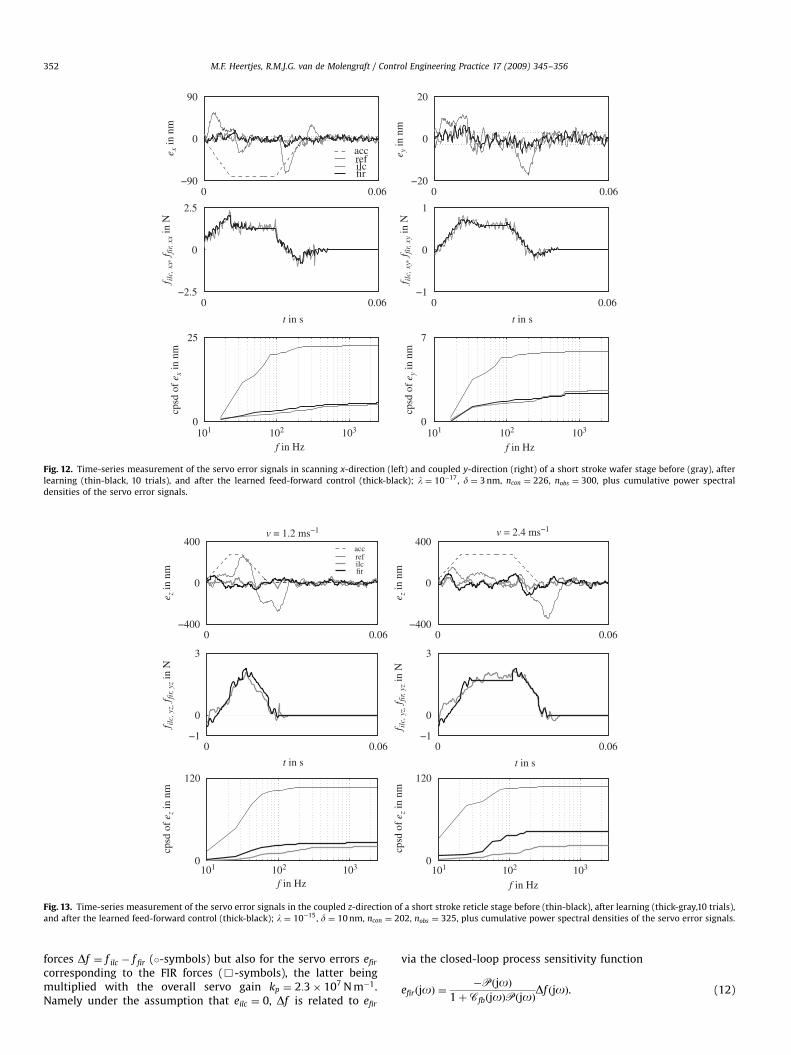
In the MIMO context of Figs. 4, 5, and 10, Fig. 12 shows theeffect of: (i) no learning, (ii) an ILC such as discussed in theprevious section, and (iii) a generalized learning control based onFIR modeling. At a short-stroke wafer stage and in the absenceof learning (ref), the effect of a single acceleration set-point in thex-axis (dashed curve) is clearly visible in terms of performancelimiting error levels and settling times, see the upper part ofthe figure. With learning (ilc), the error levels in both x andy-directions become significantly smaller. In the middle part ofthe figure, it can be seen that the ILC forces f ilc;xx and f ilc;xy clearlyrelate to the set-point characteristics and show a good corre-spondence with the generalized FIR forces f fir;xx and f fir;xy (fir). Thiscorrespondence also applies to the error responses which can beseen both in time-domain (upper part) as well as in frequency-domain (lower part), the latter via cpsd analysis.
The ability to generalize the learned forces while maintainingservo performance is considered in Fig. 13. In a cross validationexperiment where two scanning velocities are considered: v ¼
1:2 m s�1 (left part) and v ¼ 2:4 m s�1 (right part), the effect oflearning is shown in terms of improved settling behavior. Atv ¼ 2:4 m s�1, the learned forces (thick-gray) and correspondingset-point profile (dashed) are used to construct the FIR mapping.
0 0.06−2
0
1
t in s
f ilc,
f fir
in N
firilc
acc
Fig. 11. Time-series measurement of a learned force signal (thin) and the
corresponding approximation (thick) along with the acceleration profile scaled
withPnc
i¼1cðiÞ, nc ¼ 20.
On the basis of this mapping, generalized FIR forces (thick-black)are applied to the coupled z-direction of a short-stroke reticlestage. This is done at the set-point profile for which is learned butalso for the set-point profile at v ¼ 1:2 m s�1 for which in generalis not learned. Both in time-domain (upper part) as well as infrequency-domain representations (lower part), it can be seenthat the generalizing properties of the FIR approach relate to asignificant improvement in settling behavior, thereby showing areasonable match with learning at each set-point separately.
In designing an FIR filter, the number of FIR coefficients n
represents an important parameter in achieving servo perfor-mance. To study its effect, different pairs of ILC forces andcorresponding FIR models are compared, each pair related toa model based on a different number of FIR coefficientsn ¼ nc 2 f1; . . . ;55g. The corresponding FIR forces are applied toa short-stroke wafer stage. This is illustrated in Fig. 14 whereperformance is assessed through the infinity norm of the non-scanning (coupled) error signal erz . Additionally, the effect isshown at a fixed number of coefficients n ¼ 30 by time-seriesmeasurement and cpsd analysis. In a cross-validation contextcontaining two scanning velocities v ¼ 0:6 and 0:3 m s�1, it can beseen that beyond the large error reduction at n ¼ 5, only limitedextra reduction is obtained by increasing the number of FIRcoefficients. The infinity norm is minimal at n ¼ 30, beyond whichhardly any settling-induced behavior is found in the error signals.The observation that a low-order feed-forward control designsolves the performance problem to a large extent is widely-acknowledged in industrial motion control. In this regard, thegeneralized FIR forces form no exception.
Apart from the number of FIR coefficients, the data intervalused to construct the FIR mapping (this is indicated by nfirpnobs)is an important design parameter. This is because the linearmapping at hand demonstrates sensitivity to actuator/amplifiernonlinearity,1 which is encountered when changing the directionof motion, the so-called direction dependency, but also whencomparing the acceleration phase with the deceleration phasewithin a single motion. Even when comparing the positive jerk(derivative of acceleration) phase with the negative jerk phasewithin a single acceleration (or deceleration) phase. The effect isshown in Fig. 15 at a reticle stage by considering two FIRcontrollers. Each controller uses a different (but overlapping)interval of training data along the execution of the sameacceleration set-point profile. In the first interval, data is recordedfrom t ¼ 3:3� 10�3 to 5:5� 10�2 s (nfir ¼ 260) which covers theacceleration phase almost entirely. In the second interval, data isrecorded from t ¼ 3:02� 10�2 to 5:5� 10�2 s (nfir ¼ 118) whichonly contains data near the end of the acceleration phase. Fromforce time-series measurement, it becomes clear that the resultsrelated to interval 1 give a better approximation along the entireacceleration profile. Since interval 2 only takes into account datanear the end of the acceleration profile, the generalized forces atthis part of the profile are very accurate accordingly. From errortime-series measurement—this is the middle part of the figure—itis shown that the forces based on interval 2 reduce the effect ofsettling behavior beyond the acceleration phase in a way similarto the ILC forces (indicated area). By evaluating the data (throughthe infinity norm) at the constant velocity phase, it can be seenthat an optimum for nfir appears near the end of the accelerationphase (lower part). This is clear from the fact that earlier set-pointexcitation is largely excluded from the FIR mapping. As a result,the FIR forces exactly match with the ILC forces beyond this phase.The optimum is shown for the difference between the ILC and FIR
1 The amplifiers/actuators possess hysteresis as well as motor constant
variation.
ARTICLE IN PRESS
0 0.06−90
0
90
0 0.06−20
0
20
0 0.06−2.5
0
2.5
0 0.06−1
0
1
101 102 1030
25
101 102 1030
7
t in s t in s
e x in
nm
e y in
nm
f ilc,
xx,
f fir
, xx
in N
f ilc,
xy,
f fir
, xy
in N
cpsd
of
e x in
nm
cpsd
of
e y in
nm
refilcfir
acc
f in Hz f in Hz
Fig. 12. Time-series measurement of the servo error signals in scanning x-direction (left) and coupled y-direction (right) of a short stroke wafer stage before (gray), after
learning (thin-black, 10 trials), and after the learned feed-forward control (thick-black); l ¼ 10�17, d ¼ 3 nm, ncon ¼ 226, nobs ¼ 300, plus cumulative power spectral
densities of the servo error signals.
0 0.06−400
0
400
0 0.06−400
0
400
0 0.06−1
0
3
0 0.06−1
0
3
0
120
0
120
e z in
nm
e z in
nm
f ilc,
yz, f f
ir, y
z in
N
f ilc,
yz, f f
ir, y
z in
N
cpsd
of
e z in
nm
cpsd
of
e z in
nm
v = 1.2 ms−1
accrefilcfir
f in Hz f in Hz103102101103102101
t in st in s
v = 2.4 ms−1
Fig. 13. Time-series measurement of the servo error signals in the coupled z-direction of a short stroke reticle stage before (thin-black), after learning (thick-gray,10 trials),
and after the learned feed-forward control (thick-black); l ¼ 10�15, d ¼ 10 nm, ncon ¼ 202, nobs ¼ 325, plus cumulative power spectral densities of the servo error signals.
M.F. Heertjes, R.M.J.G. van de Molengraft / Control Engineering Practice 17 (2009) 345–356352
forces Df ¼ f ilc � f fir (�-symbols) but also for the servo errors efir
corresponding to the FIR forces (&-symbols), the latter beingmultiplied with the overall servo gain kp ¼ 2:3� 107 N m�1.Namely under the assumption that eilc ¼ 0, Df is related to efir
via the closed-loop process sensitivity function
efirðjoÞ ¼�PðjoÞ
1þCfbðjoÞPðjoÞDf ðjoÞ. (12)

ARTICLE IN PRESS
1 5 10 15 20 25 30 35 40 45 50 550
1
0 0.03−1
0
0.5
0 0.03−1
0
0.5
102 1030
0.6
102 1030
0.6
nc
||er z|| ∞
in �
rad
t in s
e rz in
� r
ad
e rz in
� r
ad
cpsd
of
e rz in
� r
ad
cpsd
of
e rz in
� r
ad
v = 0.6 ms−1 at n = 30 v = 0.3 ms−1 at n = 30
accreffir
fir (0.6)fir (0.3)
f in Hz f in Hz
t in s
Fig. 14. Time-series measurement of the error signal erz evaluated (and cross-validated at two different scanning speeds) through the infinity norm and using FIR learning
for a different number of FIR coefficients n 2 f1; . . . ;55g in the non-scanning direction of a short-stroke wafer stage.
0 0.06−3
0
1
0 0.06−4
0
2
0 0.06−40
0
40
0 0.06−40
0
40
0 0.040
0.6
e y in
nm
f ilc,
ffir
in N
||·|| ∞
in N
interval 1 (nfir = 260) interval 2 (nfir = 118)
interval 1 interval 2
refilcfir
t in s
Fig. 15. Sensitivity of the finite impulse response mapping to expressions of nonlinear system behavior in the learned forces for the scanning y-direction of a short stroke
reticle stage; l ¼ 10�17 m2 N�2, d ¼ 5 nm, ncon ¼ 226, nobs ¼ 275, n ¼ nc ¼ 45.
M.F. Heertjes, R.M.J.G. van de Molengraft / Control Engineering Practice 17 (2009) 345–356 353
Below the bandwidth, it follows that kefirðjoÞk � kCfbðjoÞk�1k
Df ðjoÞk. For the considered PID design this can be simplified tokefirðjoÞk � kDf ðjoÞk=kp. From Fig. 15, it is concluded that the
presence of nonlinearity can severely limit the output of themapping to resemble with the ILC forces and therefore with theILC error response.
ARTICLE IN PRESS
M.F. Heertjes, R.M.J.G. van de Molengraft / Control Engineering Practice 17 (2009) 345–356354
5. Performance assessment on a short-stroke wafer stage
To demonstrate the potential of the learned feed-forwarddesign in achieving robust performance, an industrial perfor-mance assessment is conducted on a short-stroke wafer stage.In the analysis, robustness to set-point variation is tested byincluding different die sizes and scan velocities. Performance isevaluated in terms of settling-time reduction. In this regard, twoindustrial performance measures are considered: the movingaverage filter operation and the moving standard deviation filteroperation (Heertjes & Van de Wouw, 2006).
The moving average filter operation expresses the level ofposition accuracy that can be obtained during the process of waferscanning. It has a strong relation with so-called scanning overlay(see also Bode et al., 2004) and is defined as
MaðiÞ ¼1
nwin
Xiþnwin=2�1
j¼i�nwin=2
eðjÞ; 8i 2 Z, (13)
with nwin 2 N an application specific time frame. This filteroperation basically represents a low-pass filtering of the error
00.35
0.7
0
20
400
30
60
die size in mmscan velocity in ms−
1
||ex||
∞ in
nm
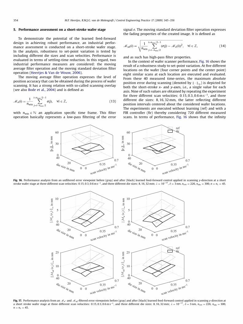
Fig. 16. Performance analysis from an unfiltered error viewpoint before (gray) and aft
stroke wafer stage at three different scan velocities: 0:15;0:3;0:6 m s�1, and three differe
00.35
0.7
0
20
400
5
10
00.35
0.7
0
20
400
10
25
die size in mm
die size in mm
scan velocity in ms−1
scan velocity in ms−1
a (e
x)∞
in n
msd
(e x
)∞
in n
m
Fig. 17. Performance analysis from an Ma- and Msd-filtered error viewpoints before (gra
a short stroke wafer stage at three different scan velocities: 0:15;0:3;0:6 m s�1, and th
n ¼ nc ¼ 45.
signal e. The moving standard deviation filter operation expressesthe fading properties of the created image. It is defined as
MsdðiÞ ¼
ffiffiffiffiffiffiffiffiffiffiffiffiffiffiffiffiffiffiffiffiffiffiffiffiffiffiffiffiffiffiffiffiffiffiffiffiffiffiffiffiffiffiffiffiffiffiffiffiffiffiffiffiffiffiffiffiffiffiffi1
nwin
Xiþnwin=2�1
j¼i�nwin=2
ðeðjÞ �MaðiÞÞ2
vuut ; 8i 2 Z, (14)
and as such has high-pass filter properties.In the context of wafer scanner performance, Fig. 16 shows the
result of a robustness study to set-point variation. At five differentlocations on the wafer (four corner points and the center point)eight similar scans at each location are executed and evaluated.From these 40 measured time-series, the maximum absoluteposition error during scanning (denoted by k � k1) is depicted forboth the short-stroke x- and y-axes, i.e., a single value for eachaxis. Nine of such values are obtained by repeating the experimentfor three different scan velocities: 0:15;0:3;0:6 m s�1, and threedifferent die sizes: 8;16;32 mm, the latter reflecting differentposition intervals centered about the considered wafer locations.The experiments are executed without learning (ref) and with aFIR controller (fir) thereby considering 720 different measuredscans. In terms of performance, Fig. 16 shows that the infinity
00.35
0.7
0
20
400
30
60reffir
die size in mmscan velocity in ms−
1
||ey||
∞ in
nm
er (black) learned feed-forward control applied in scanning y-direction at a short
nt die sizes: 8;16;32 mm; l ¼ 10�17, d ¼ 3 nm, ncon ¼ 226, nobs ¼ 300, n ¼ nc ¼ 45.
00.35
0.7
0
20
400
5
10
00.35
0.7
0
20
400
10
25 firref
die size in mm
die size in mm
scan velocity in ms−1
scan velocity in ms−1
a (e
y)∞
in n
msd
(e y
)∞
in n
m
y) and after (black) learned feed-forward control applied in scanning y-direction at
ree different die sizes: 8;16;32 mm; l ¼ 10�17, d ¼ 3 nm, ncon ¼ 226, nobs ¼ 300,

ARTICLE IN PRESS
M.F. Heertjes, R.M.J.G. van de Molengraft / Control Engineering Practice 17 (2009) 345–356 355
norm of the error, which is mainly induced by the settlingphenomenon, is significantly reduced under the given MIMOlearned feed-forward; the case without learning demonstrateswhat is obtained under model-based SISO feed-forward control. Interms of scan velocity and die size variation, Fig. 16 shows limitedsensitivity, hence sufficient robustness, along the consideredparameter plane.
Performance in terms of Ma and Msd is considered in Fig. 17. Itshows that small scan velocities give rise to small error levels.Apart from the reduced amount of excitation related to suchvelocities, this is clear from the fact that nwinscan velocity�1.Decreasing the scan velocity increases nwin which in Eqs. (13)and (14) has the effect of averaging out the settling phenomenon.Figs. 16 and 17 clearly demonstrate the ability of the generalizedlearned forces to achieve robust performance.
6. Conclusions
For industrial wafer scanners, learning control provides a power-ful means to improve upon settling performance. The generalizationof the learned forces through FIR modeling adds the necessaryrobustness to set-point variation which would otherwise severelylimit the benefits of learning. This is because the wafer scanningindustry lacks an exact repetition of set-points and demands a first-time-right strategy during scanning.
In an MIMO learned feed-forward context, the occurrenceof settling behavior, one of the major servo limitations on waferthroughput, is shown to effectively disappear. Contrarily, the FIRapproach appears sensitive in the presence of nonlinear systembehavior. This avoids posing a general design rule regarding thedata interval needed to construct the FIR mapping. Regarding thenumber of FIR coefficients, a design argument other than keepingits number small cannot be deduced from the considered cross-validation experiments.
The FIR approach shows a good robustness to set-point variationwhereas servo performance is not severely compromised whencompared to the application of the ILC forces at the set-point forwhich is learned. This is the outcome of a cross validationexperiment. At the same time, the FIR approach demonstrates itsability to achieve performance in an industrial environment. In thisregard, the approach shows potential in the broader context ofindustrial motion control systems.
Appendix
The proof of Theorem 1 is given as follows. By adopting thenotation ailcðkþ nncÞ ¼ an, it follows from (8) that
ATilcAilc ¼
a2n þ � � � þ a2
nþo�1 % ::: %
an�1an þ � � � þ anþo�2anþo�1 a2n�1 þ � � � þ a2
nþo�2 ::: %
..
. ... . .
. ...
a1an þ � � � þ aoanþo�1 a1an�1 þ � � � þ aoanþo�2 ::: a21 þ :::þ a2
o
2666664
3777775
,
(15)
where % indicates the symmetric counterparts. Invertibility of(15) implies that all columns are independent. Consider the firstand the second column, or
a2n þ � � � þ a2
nþo�1 an�1an þ � � � þ anþo�2anþo�1
an�1an þ � � � þ anþo�2anþo�1 a2n�1 þ :::þ a2
nþo�2
..
. ...
2664
3775.
(16)
In view of symmetry, both columns are independent if the twodiagonal terms differ. In fact, this holds true for each consecutive
pair of columns, i.e., the second and the third, the third and thefourth, and so on. If both diagonal terms are equal, or
a2n þ � � � þ a2
nþo�1 ¼ a2n�1 þ � � � þ a2
nþo�2 ) a2n�1 ¼ a2
nþo�1, (17)
independency results from the fact that the symmetric off-diagonal terms differ from the diagonal terms. Namely assumeall four terms in (16) are equal, or
a2n þ � � � þ a2
nþo�1 ¼ an�1an þ � � � þ anþo�2anþo�1
¼ 12a2
n þ � � � þ12a2
nþo�1 þ12a2
n�1 þ � � � þ12a2
nþo�2
� 12ðan � an�1Þ
2� � � � � 1
2ðanþo�1 � anþo�2Þ2.
(18)
Then (18) combined with (17) gives
�12a2
n�1 þ12a2
nþo�1 ¼ �12ðan � an�1Þ
2� � � � � 1
2ðanþo�1 � anþo�2Þ2¼ 0,
(19)
or an � an�1 ¼ � � � ¼ anþo�1 � anþo�2 ¼ 0, which under the assump-tion that ailcðkþ nncÞ ¼ ana0, reduces to an�1 ¼ an ¼ � � � ¼
anþo�1a0. But this contradicts the earlier assumption that Ailc
contains no columns with o equal entries. Hence the symmetricoff-diagonal terms differ from the diagonal terms rendering thecolumns in (16) independent. The remainder of the proof followsfrom repeating the previous steps for each consecutive pair ofcolumns.
References
Ahn, H.-S., Moore, K. L., & Chen, Y. Q. (2006). Monotonic convergent iterativelearning controller design based on interval model conversion. IEEE Transac-tions on Automatic Control, 51(2), 366–371.
Baggen, M., Heertjes, M. F., & Kamidi, R. (2008). Data-based feedforward control inMIMO motion systems. In Proceedings of the American control conference,Seattle, WA (pp. 3011–3016).
Bode, C. A., Ko, B. S., & Edgar, T. F. (2004). Run-to-run control and performancemonitoring of overlay in semiconductor manufacturing. Control EngineeringPractice, 12, 893–900.
Bristow, D. A., Tharayil, M., & Alleyne, A. G. (2006). A survey of iterative learningcontrol—A learning-based method for high-performance tracking. IEEE ControlSystems Magazine, 96–114.
Cai, Z., Freeman, C. T., Lewin, P. L., & Rogers, E. (2008). Iterative learning control fora non-minimum phase plant based on a reference shift algorithm. ControlEngineering Practice, 16, 633–643.
Chen, C. K., & Hwang, J. (2005). Iterative learning control for position tracking of apneumatic actuated X–Y table. Control Engineering Practice, 13(12), 1455–1461.
Chen, Y. Q., Moore, K. L., Yu, J., & Zhang, T. (2008). Iterative learning control andrepetitive control in hard disk drive industry—A tutorial. International Journalof Adaptive Control and Signal Processing, 22(4), 325–343.
Dijkstra, B. G., & Bosgra, O. H. (2002). Extrapolation of optimal lifted system ILCsolution, with application to a waferstage. In Proceedings of the Americancontrol conference, Anchorage, AK (pp. 2595–2600).
Dixon, W. E., & Chen, J. (2003). Comments on ‘‘A composite energy function-basedlearning control approach for nonlinear systems with time-varying parametricuncertainties’’. IEEE Transactions on Automatic Control, 48(9), 1671–1672.
Ghosh, J., & Paden, B. (2002). A pseudoinverse-based iterative learning control. IEEETransactions on Automatic Control, 47(5), 831–837.
Groot-Wassink, M., Van de Wal, M., Scherer, C., & Bosgra, O. (2005). LPV control fora wafer stage: Beyond the theoretical solution. Control Engineering Practice, 13,231–245.
Gunnarsson, S., & Norrlof, M. (2001). On the design of ILC algorithms usingoptimization. Automatica, 37, 2011–2016.
Heertjes, M. F., & Tso, T. (2007a). Nonlinear iterative learning control withapplications to lithographic machinery. Control Engineering Practice, 15,1545–1555.
Heertjes, M. F., & Tso, T. (2007b). Robustness, convergence, and Lyapunov stabilityof a nonlinear iterative learning control aplied at a wafer scanner. InProceedings of the American control conference, New York, WA (pp. 5490–5495).
Heertjes, M. F., & Van de Wouw, N. (2006). Variable control design and itsapplication to wafer scanners. In Proceedings of conference on decision andcontrol, San Diego, CA (pp. 3724–3729).
Mishra, S., Coaplen, J., & Tomizuka, M. (2007). Precision positioning of waferscanners; segmented iterative learning control for nonrepetitive disturbances.IEEE Control Systems Magazine, August, 20–25.
Moore, K. L. (1999). An iterative learning control algorithm for systems withmeasurement noise. In Proceedings of the conference on decision and control,Phoenix, AZ (pp. 270–275).

ARTICLE IN PRESS
M.F. Heertjes, R.M.J.G. van de Molengraft / Control Engineering Practice 17 (2009) 345–356356
Moore, K. L., Chen, Y. Q., & Bahl, V. (2005). Monotonically convergent iterativelearning control for linear discrete-time systems. Automatica, 41, 1529–1537.
Potsaid, B., & Wen, J. (2004). High performance motion tracking control. InProceedings of the 2004 IEEE international conference on control applications,Taipei, Taiwan (pp. 718–723).
Rotariu, I., Dijkstra, B. G., & Steinbuch, M. (2004). Comparison of standard and liftedILC on a motion system. In Proceedings of the third IFAC symposium onmechatronic systems, Sydney, Australia.
Rotariu, I., Ellenbroek, R., & Steinbuch, M. (2003). Time–frequency analysis of amotion system with learning control. In IEEE Proceedings of the Americancontrol conference, Denver, CO (pp. 3650–3654).
Rotariu, I., Ellenbroek, R., Van Baars, G., & Steinbuch, M. (2003). Iterative learningcontrol for variable setpoints, applied to a motion system. In Proceedings of theEuropean control conference, Cambridge, UK (pp. 2732–2739).
Tayebi, A., & Islam, S. (2006). Adaptive iterative learning control for robotmanipulators: Experimental results. Control Engineering Practice, 14(7),843–851.
Tousain, R. L., & Van der Meche, E. (2001). Design strategies for iterative learningcontrol based on optimal control. In Proceedings of the 40th conference ondecision and control, Orlando, FL (pp. 4463–4468).
Van de Wal, M., Van Baars, G., Sperling, F., & Bosgra, O. (2002). MultivariableH1=m feedback control design for high-precision wafer stage motion. ControlEngineering Practice, 10, 739–755.
Van der Meulen, S. H., Tousain, R. L., & Bosgra, O. H. (2008). Fixed structurefeedforward controller design exploiting iterative trials: Application to a waferstage and a desktop printer. Journal of Dynamic Systems, Measurement, andControl, 130(051006), 1–16.
Xu, J.-X. (1998). Direct learning of control efforts for trajectories with different timescales. IEEE Transactions on Automatic Control, 43(7), 1027–1030.
Xu, J.-X., & Tan, Y. (2002). A composite energy function-based learning controlapproach for nonlinear systems with time-varying parametric uncertainties.IEEE Transactions on Automatic Control, 47(11), 1940–1945.
Xu, J.-X., & Tan, Y. (2003). Author’s reply. IEEE Transactions on Automatic Control,48(9), 1672–1674.