i_'': _:_i

Applications of Artificial Neural Networks in Structural

Engineering with Emphasis on Continuum Models

by Rakesh K. Kapania* and Youhua Liu**

Department of Aerospace and Ocean Engineering

Virginia Polytechnic Institute and State University

Blacksburg, VA 24061-0203

June, 1998

.: Professor

**: Graduate Research Assistant

Abstract

The use of continuum models for the analysis of discrete built-up complex aerospace struc-

tures is an attractive idea especially at the conceptual and preliminary design stages. But

the diversityof available continuum models and hard-to-use qualities of these models have

prevented them from finding wide applications. In this regard, Artificial Neural Networks

(ANN or NN) may have a great potential as these networks are universal approximators

that can realize any continuous mapping, and can provide general mechanisms for building

models from data whose input-output relationship can be highly nonlinear.

The ultimate aim of the present work is to be able to build high fidelity continuum models

for complex aerospace structures using the ANN. As a first step, the concepts and features

of ANN are familarized through the MATLAB NN Toolbox by simulating some represen-

tative mapping examples, including some problems in structural engineering. Then some

further aspects and lessons learned about the NN training are discussed, including the

performances of Feed-Forward and Radial Basis Function NN when dealing with noise-

polluted data and the technique of cross-validation. Finally, as an example of using NN in

continuum models, a lattice structure with repeating cells is represented by a continuum

beam whose properties are provided by neural networks.

1. Introduction

It is estimated that about 90_ of the cost of an aerospace product is committed

during the first 10% of the design cycle. As a result, the aerospace industry is increasingly

coming to the conclusion that physics-based high fidelity models (Finite Element Analysis

for structures, Computational Fluid Dynamics for aerodynamic loads etc.) need to be used

earlier at the conceptual design stage, not only at a subsequent preliminary design stage.

But an obstacle to using the high fidelity models at the conceptual level is the high CPU

time that are typically needed for these models, despite the enormous progress that has

been made in both the computer hardware and software.

During the late seventies and early eighties, there was a significant interest in

obtaining continuum models to represent discreet built-up complex lattice, wing, and

laminated wing structures. These models use very few parameters to express the original

structure geometry and layout. The initial model generation and set-up is fast as com-

pared to a full finite element model. Assembly of stiffness and mass matrices and solution

times for static deformation and stresses or natural modes are significantly less than those

needed in a finite element analysis. All these make continuum models very attractive for

preliminary design and optimization studies.

Despite its great potential, the continuum approach has gained a limited popu-

larity in the aerospace designers community. This is, perhaps, due to the fact that all

the developments have been made by keeping specific examples (eg. periodic lattices or

specific wings) in mind. Also, with some exceptions, most of these approaches were rather

complex. The key obstacle though appears to be the fact that if the designer makes a

change in the actual built-up structures, the continuum model has to be determined from

2

scratch.

The complex nature of the various methods and the large number of problems

encountered in determining the equivalent models are not surprising given the fact that

determining these models for a given complex structure (a large space structure or a wing)

belongs to a class of problems called inverse problems. These problems are inherently ill-

posed and it is fruitless to attempt to determine unique continuum models. The present

work deals with investigating the possibility that a more rational and efficient approach

of determining the continuum models can be achieved by using artificial neural networks.

The working mechanism in brains of biological creatures has long been an area of

intense study. It was found around the first decade of this century that neurons (nerve

cells) are the structural constituents of the brain. The neurons interact with each other

through synapses, and are connected by axons (transmitting lines) and dentrites (receiv-

ing branches). It is estimated that there are on the order of 10 billion neurons in the

human cortex, and about 60 trillion synapses (Ref. 1). Although neurons are 5,-_6 orders

of magnitude slower than silicon logic gates, the organization of them is such that the

brain has the capability of performing certain tasks (for example, pattern recognition, and

motor control etc.) much faster than the fastest digital computer nowadays. Besides, the

energetic efficiency of the brain is about 10 orders of magnitude lower than the best com-

puter today. So it can be said, in the sense that a computer is an information-processing

system, the brain is a highly complex, nonlinear, and efficient parallel computer.

Artificial Neural Networks (ANN), or simply Neural Networks (NN) are compu-

tational systems inspired by the biological brain in their structure, data processing and

restoring method, and learning ability. More specifically, a neural network is defined as

a massively parallel distributed processor that has a natural propensity for storing ex-

periential knowledgeand making it available for future use by resembling the brain in

two aspects: (a) Knowledge is acquired by the network through a learning process; (b)

Inter-neuron connectionstrengthsknown assynaptic weights (or simply weights) are used

to store the knowledge(Ref. 1).

With a history traced to the early 1940s,and two periods of major increasesin

researchactivities in the early 1960sand after the mid-1980s.ANNs havenow evolved to

be a mature branch in the computational scienceand engineeringwith a large number

of publications, a lot of quite different methods and algorithms and many commercial

software and some hardware. They have found numerous applications in scienceand

engineering, from biological and medical sciences,to information technologies such as

artificial intelligence,pattern recognition, signalprocessingand control, and to engineering

areasas civil and structural engineering.

In this report a brief description is given to the most extensively used neural net-

work in civil and structural engineering,Multi-Layer Feed-ForwardNN, and another kind

of NN, Radial Basis Function NN, which is very efficient in somecases. Someconcep-

tional features of NN are listed. Someexamplesof the application of neural network are

given, among which severalare published real problems in civil and structural engineer-

ing. Based on our experienceof using the MATLAB NN Toolbox, some important and

very practical issueson the application of NN will be brought out.

Then a section of the report is dedicated to the developmentof algorithms car-

rying out the very useful concept of cross-validation. Through the results for several

examplesobtained from the algorithms, someobservationson issuessuchasover-training

and network complexity are given.

4

In the last section an exampleof using NN in continuum models is given. A lattice

structure with repeating cells is represented_, a continuum beam whoseproperties, as

functions of the repeating cell particulars, are provided by neural networks.

2. Examples of NN

As simplified models of the biological brain, ANNs have lots of variations due

to specific requirements of their tasks by adopting different degree of network complex-

ity, type of inter-connection, choice of transfer function, and even differences in training

method.

According to the types of network, there are Single Neuron network (1-input 1-

output, no hidden layer), Single-Layer NN or Percepton (no hidden layer), and Multi-

Layer NN (1 or more hidden layers). According to the types of inter-connnection, there

are Feed-Forward network (values can only be sent from neurons of a layer to the next

layer), Feed-Backward network (values can only be sent in the different direction, i.e.

from the present layer to the previous layer), and Recurrent network (values can be sent

in both directions).

In the following a brief description is given to two kinds of extensively used neural

networks and some of the pertinent concepts.

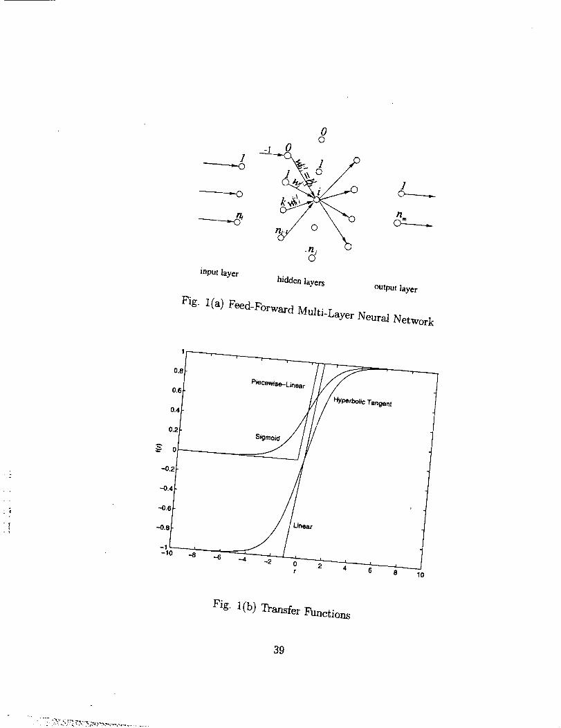
2.1 Feed-Forward Multi-layer Neural Network

As shown in Fig. l(a), in the j-th layer, the i-th neural has inputs from the

(j - l)-th layer of value _-l(k = 1, ...,nj_l), and has the following output

5

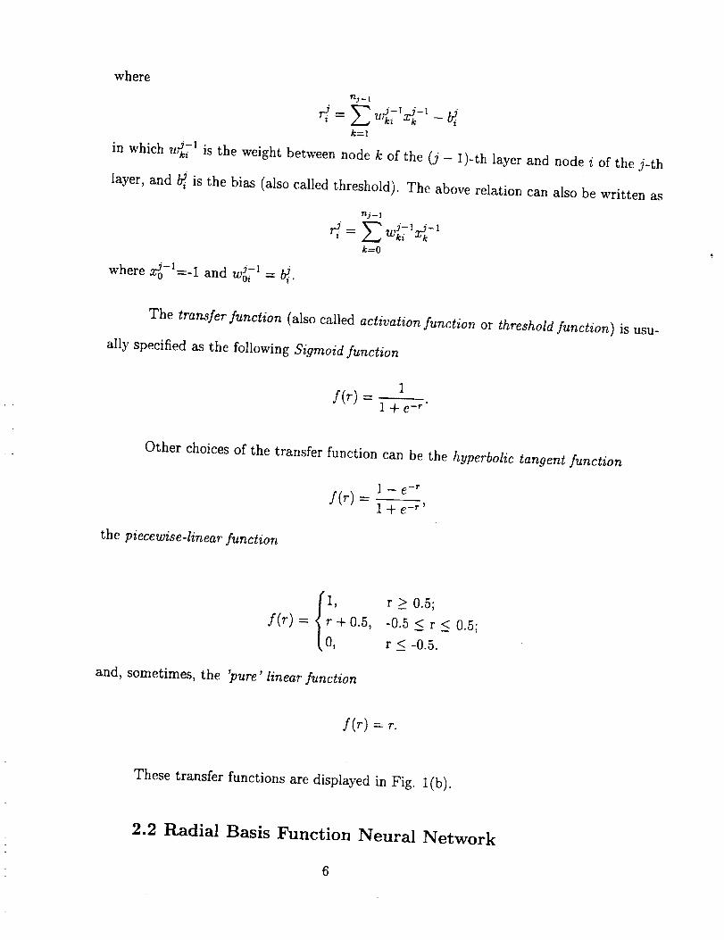
where

nj _ lj 1

_ j--1 "-ri

k=l

j-1 is the weight between node k of the (j - 1)-th layer and node i of the j-thin which w_i

layer, and _ is the bias (also called threshold). The above relation can also be written as

n j- 1

"Wki X k

k---0

• j-1 = _.where _0-1 =- I and Woi

The transfer function (also called activation function or threshold function) is usu-

all), specified as the following Sigmoid function

1

f(r) -- 1 + e-r"

Other choices of the transfer function can be the hyperbolic tangent function

1 _ e -r

f(r) = 1+ e-r'

the piecewise-linear function

and, sometimes, the 'pure

1,f(r) = r + 0.5,

0,

' linear function

r _> 0.5;

-0.5 < r _< 0.5;

r < -0.5.

f(r) =r.

These transfer functions are displayed in Fig. l(b).

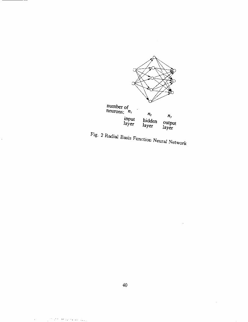
2.2 Radial Basis Function Neural Network

6

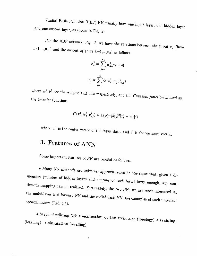
Radial Basis Function (RBF) NN usually have one input layer, one hidden layer

and one output layer, asshown in Fig. 2.

I (hereFor the RBF network, Fig. 2, we have the relations betweenthe input x i

i=l,...,nl ) and the output x_ (here k=l,...,n3) as follows.

n2

j=i

rj = a(z_, w¢,b,j)

where w 2, b2 are the weights and bias respectively, and the Gaussian function is used as

the transfer function:

1 b 1 [b_ ]2a(x:, wj, ,,;1= _xp(-t ,o_ [x_- w_?)

where w _ is the center vector of the input data, and b 1 is the variance vector.

3. Features of ANN

Some important features of NN are briefed as follows.

,, Many NN methods are universal approximators, in the sense that, given a di-

mension (number of hidden layers and neurons of each layer) large enough, any con-

tinuous mapping can be realized. Fortunately, the two NNs we are most interested in,

the multi-layer feed-forward NN and the radial basis NN, are examples of such universal

approximators (Ref. 4,5).

,, Steps of utilizing NN: specification of the structure (topology)--+ training

(learning) _ simulation (recalling).

7

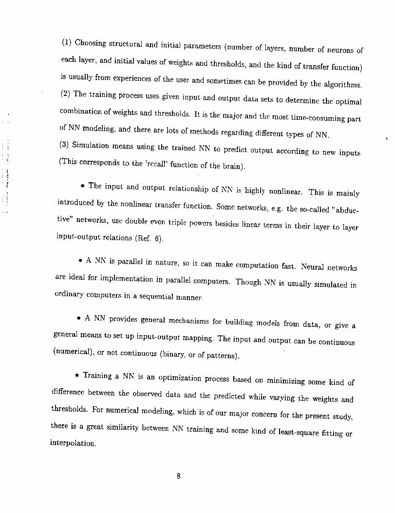
(1) Choosing structural and initial parameters (number of layers, number of neuronsof

eachlayer, and initial valuesof weights and thresholds,and the kind of transfer function)

is usually from experiencesof the userand sometimescanbe provided by the algorithms.

(2) The training processusesgiven input and output data sets to determine the optimal

combination of weightsand thresholds. It is the major and the most time-consuming part

of NN modeling, and there are lots of methods regarding different types of NN.

(3) Simulation means using the trained NN to predict output according to new inputs

(This correspondsto the 'recall' function of the brain).

• The input and output relationship of NN is highly nonlinear. This is mainly

introduced by the nonlinear transfer function. Some networks, e.g. the so-called "abduc-

tive" networks, use double even triple powers besides linear terms in their layer to layer

input-output relations (Ref. 6).

• ANN is parallel in nature, so it can make computation fast. Neural networks

are ideal for implementation in parallel computers. Though NN is usually simulated in

ordinary computers in a sequential manner.

• ANN provides general mechanisms for building models from data, or give a

general means to set up input-output mapping. The input and output can be continuous

(numerical), or not continuous (binary, or of patterns).

• Training a NN is an optimization process based on minimizing some kind of

difference between the observed data and the predicted while varying the weights and

thresholds. For numerical modeling, which is of our major concern for the present study,

there is a great similarity between NN training and some kind of least-square fitting or

interpolation.

8

• Where and when to useNN depend on the situation, and NN is not a panacea.

The following comment on NN application on structural engineeringseemingly can be

generalizedin other areas:

"The real usefulness of neural networks in structural engineering is not in repro-

ducing existing algorithmic approaches .for predicting structural responses, as a computa-

tionally efficient alternative, but in providing concise relationships that capture previous

design and analysis experiences that are useful for making design decisions" (Ref. 9).

4. Algorithms

Toolbox

in the MATLAB Neural Network

When using MATLAB NN Toolbox, one should first choose the number of input and

output variables. This is accomplished by specifying the two matrices p and t; where p is

a m× n matrix; m is the number of input variables, and n the number of sets of training

data; and t is a l×n matrix; I is the number of output variables. Then the number of

network layers, and numbers of neurons of each layer should be specified.

MATLAB gives algorithms for specifying initial values of weights and thresholds in

order that training can be started. For feed-forward NN, function initff is given for this

purpose. The following is an example of using the algorithm

[w l , b l , w2, b 2, w3, b3]-initff (p , n l , 'logsig ', n2, 'logsig ',t, 'logsig ') ;

where wl, w2, w3 are initial values for the weight matrices of the 1st (hidden), 2nd

(hidden) and 3rd (output) layer respectively, bl, b2, b3 are the bias (threshold) vectors,

nl and n2 the number of neurons in the 1st and 2nd hidden layer respectively, and 'Iogsig'

9

meansthat the Sigmoid transfer function is used.

The presentversionof MATLAB NN Toolbox cansupport only 2 hidden layers,but

the number of neurons is only limited by the available memory of the computer system

being used. For the transfer function, one can also use other choices,such as 'tansig'

(hyperbolic tangent sigmoid), 'radbas' (radial basis) and 'purelin' (linear) etc.

Experiences of using initff indicated that it seems to be a random process since

it is found that the result of the execution of this algorithm each time is different. And

other conditions kept the same, two execution of this function usually give quite different

converging histories of training by the training algorithm (see Fig. 3 (a) and (b)). We

shall discuss this later in 6.3.

Shown in the following is the MATLAB algorithm for training feed-forward network

with back-propagation:

[wl, bl, w2, b2, w3, b3, ep, tr]=trainbp (wl, bl, 'logsig ', w2, b2, 'logsig ', w3, b3, 'logsig ',p, t, tp);

where most of the parameters which the user should take care of have been mentioned

in the above paragraphs• The only set of parameters that the user sometimes need to

specify is the 1 x4 vector tp , where the first element indicates the number of iterations

between updating displays, the second the maximum number of iterations of training after

which the algorithm terminates the training process, the third the converging criterion

(sum-squared error goal), and the last being the learning rate. The default value of tp is

[25,loo,0.02,o.ol].

Other algorithms for training: trainbpa (train feed-forward NN with back-propagation

and adaptive learning), solverb (design and train radial basis network), and trainlm (train

10

feed-forwardNN with Levenberg-Marquardt) etc.

trainbpa and trainlm have very similar formats for using as that of trainbp.

radial basis network designing and training algorithm has the following format

The

[wl, b i, w2, b2, nr, err]---solverb (p, t, tp).

where the algorithm chooses centers for the Gaussians and increases the neuron number

of the hidden layer automatically if the training cannot converge to the given error goal.

So it is also a designing algorithm.

After the NN is trained, one can predict output from input by using simulation

algorithms in terms of the obtained parameters wl, bl, w2, b2, etc. For feed-forward

network one use

y=simu ff (x, w I , b l , 'logsig ', w2, b2, 'logsig ')

where x is the input matrix, and y the predicted output matrix. Similarly, after a radial

basis network has been trained one uses

y--simurb (x, w l , bl , w2, b2)

to predict the output.

Once a NN is trained, we can use the formulations in 2.1 or 2.2 together with the

obtained parameters (weights etc.) to setup the network to do prediction anywhere and

not necessarily within the MATLAB environment.

11

5. Examples of Application Using MATLAB Neu-

ral Network Toolbox

5.1 A Single Input Single Output Function

The training data set are

p=[0.1, 0.2, 0.3, 0.4, 0.5, 06, 0.7, 0.8, 0.9, 1.0];

t=[o.01, o.o4, 0.09, 0.16, 0.25, 0.36, 0.49, 0.36, 0.25, 0.16];

A 1-9-1 (a input layer with 1 input, a hidden layer with 9 neurons, and an output

layer with 1 output) feed-forward NN was trained with trainbp. The comparison between

the desired (with symbol '+') and the predicted (smooth line) values and the training

history are shown in Figs. 4 (a) and (b) respectively. Another 1-9-6-1 (an input layer

with 1 input, two hidden layer with 9 and 6 neurons respectively, and a output layer with

1 output) feed-forward NN was also trained, and the comparison between the desired

values and the predicted values and the training history are shown in Figs. 5 (a) and (b),

respectively.

By adjusting the learning rate according to the circumstances, adaptive learning

usally can give better results than with a constant learning rate 'specified before the

training begins, as displayed in Fig. 6 (a) and (b). In Fig. 6 (b), the dotted curve is the

variation of learning rate, and the continuous curve is the variation of error.

5.2 Training of Multiple Variable Mappings

A multi-variable mapping is much more complicated than a single input single

12

output function. If wesay for the single input singleoutput function in Sect. 5.1, 10sets

of data can give a somewhat completedescription of the relation betweenthe input and

the output, for a mapping with k input variables and one output variable, we will need

10 k sets of data to obtain the same degree of completeness of description. That means

the efforts of training a neural network to simulate a multiple variable mapping increases

exponentially with the number of input variables.

For many practical cases, one must obtain a multiple variable mapping from a quite

limited data set. The worse is, the data are usually randomly distributed in the input

domain, rather than distributed uniformly as in the cases of experiments designed by the

DOF (degree of freedom) method. It will be of interest to know the behaviors of NNs for

such kind of data.

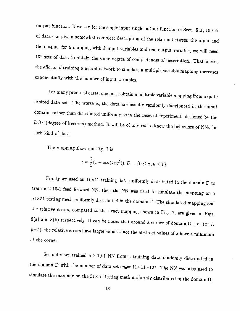
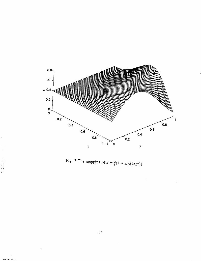
The mapping shown in Fig. 7 is

z = 2(1 + sin(4xy2)),D = {0 < x,y <_ 1}.

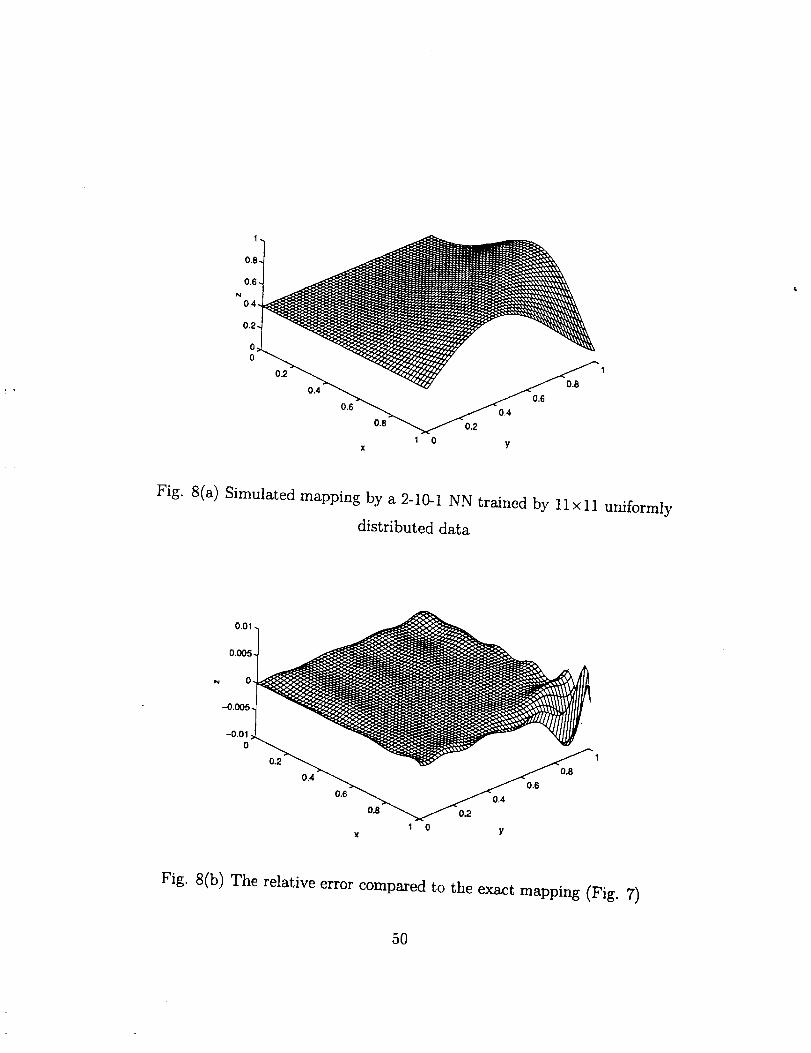
Firstly we used an 11 xll training data uniformly distributed in the domain D to

train a 2-10-1 feed forward NN, then the NN was used to simulate the mapping on a

51 x51 testing mesh uniformly distributed in the domain D. The simulated mapping and

the relative errors, compared to the exact mapping shown in Fig..7, are given in Figs.

8(a) and 8(b) respectively. It can be noted that around a corner of domain D, i.e. (x=l,

y--1 ), the relative errors have larger values since the abstract values of z have a minimum

at the corner.

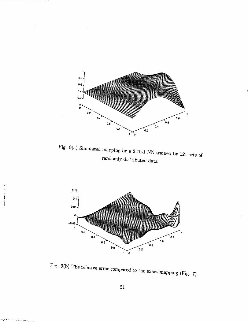
Secondly we trained a 2-10-1 NN froma training data randomly distributed in

the domain D with the number of data sets no- 11x11=121. The NN was also used to

simulate the mapping on the 51x51 testing mesh uniformly distributed in the domain D,

13

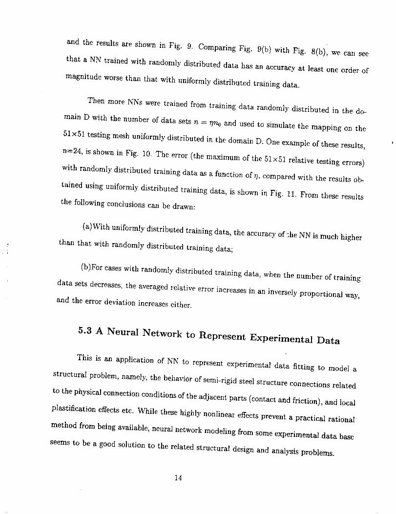
and the results are shown in Fig. 9. Comparing Fig. 9(b) with Fig. 8(b), we can see

that a NN trained with randomly distributed data has an accuracy at least one order of

magnitude worsethan that with uniformly distributed training data.

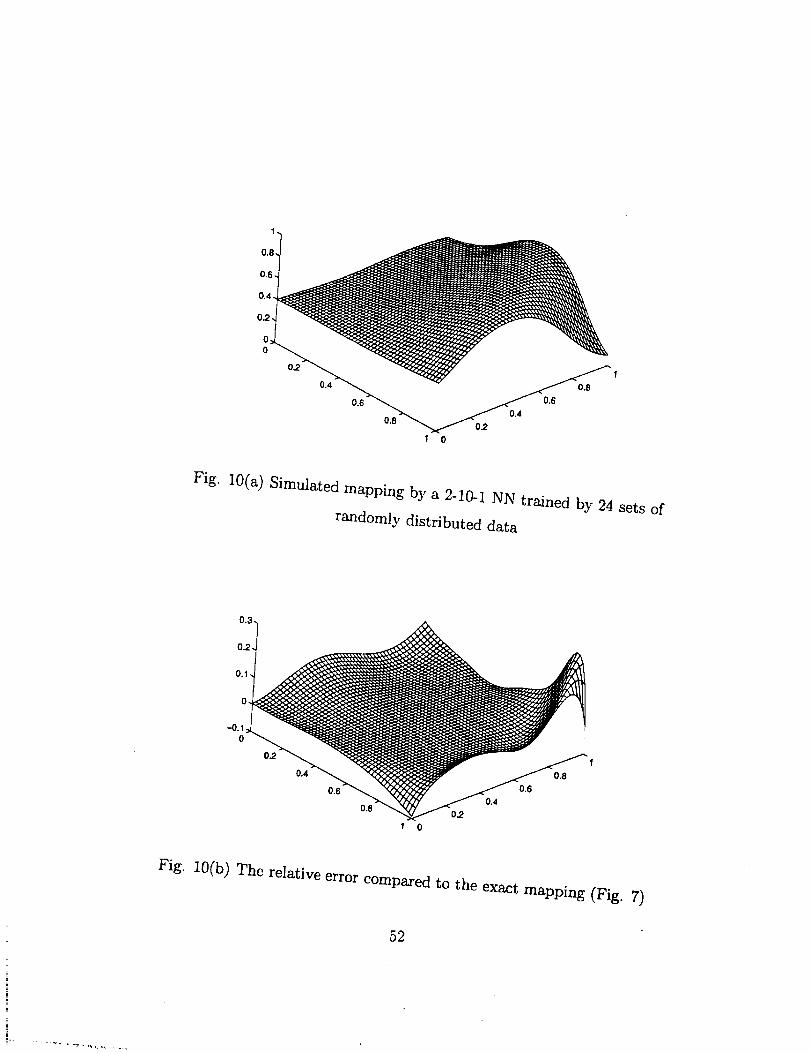
Then more NNs were trained from training data randomly distributed in the do-

main D with the number of data sets n - 77n0 and used to simulate the mapping on the

51x51 testing mesh uniformly distributed in the domain D. One example of these results,

n=24, is shown in Fig. 10. The error (the maximum of the 51x51 relative testing errors)

with randomly distributed training data as a function of r/, compared with the results ob-

tained using uniformly distributed training data, is shown in Fig. 11. From these results

the following conclusions can be drawn:

(a)With uniformly distributed training data, the accuracy of the NN is much higher

than that with randomly distributed training data;

(b)For cases with random]y distributed training data, when the number of training

data sets decreases, the averaged relative error increases in an inversely proportional way,

and the error deviation increases either.

5.3 A Neural Network to Represent Experimental Data

This is an application of NN to represent experimental data fitting to model a

structural problem, namely, the behavior of semi-rigid steel structure connections related

to the physical connection conditions of the adjacent parts (contact and friction), and local

plastification effects etc. While these highly nonlinear effects prevent a practical rational

method from being available, neural network modeling from some experimental data base

seems to be a good solution to the related structural design and analysis problems.

14

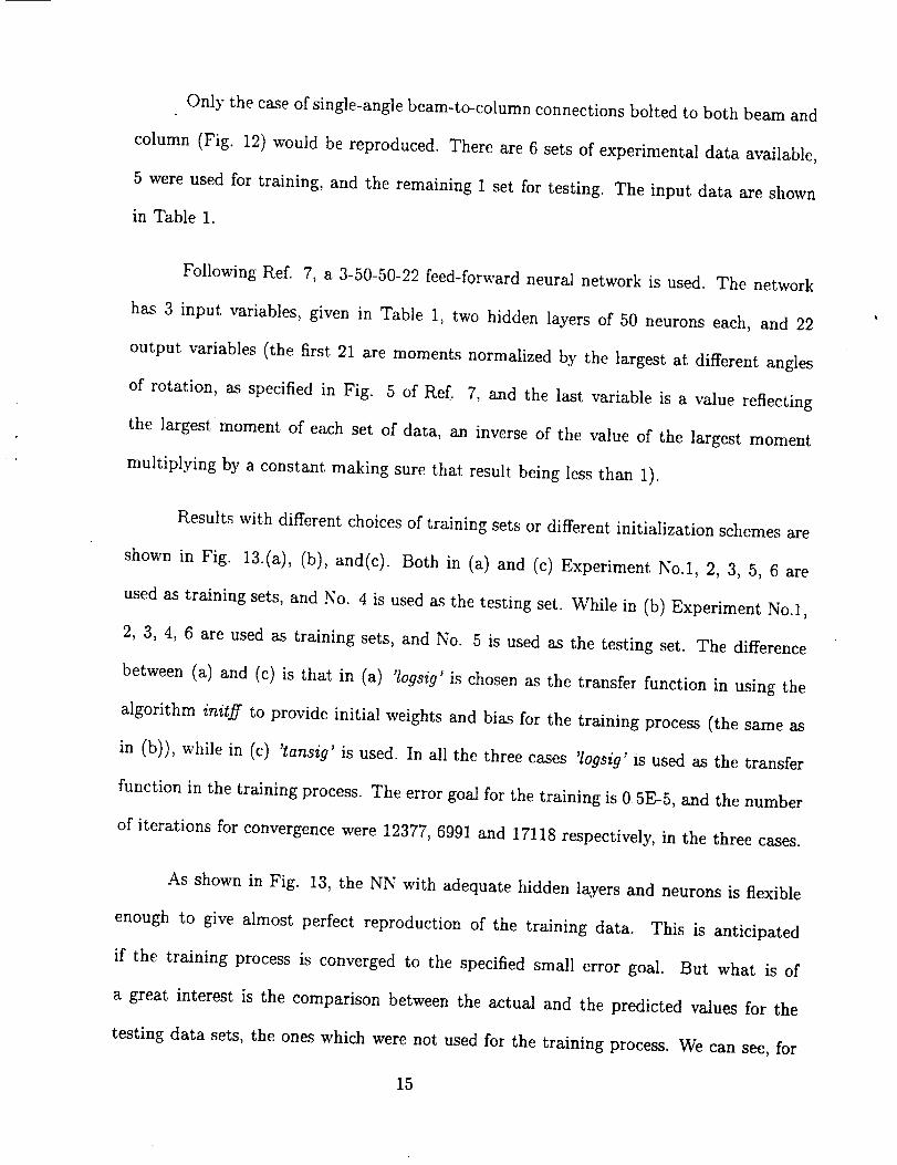
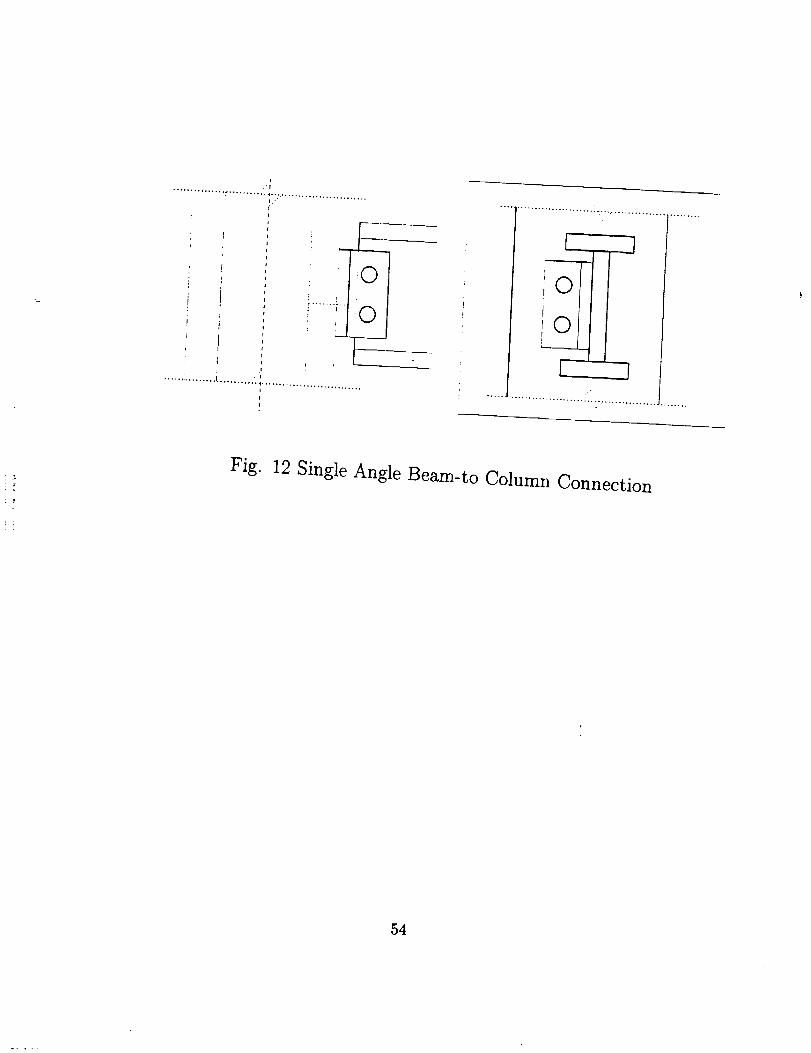
Only the caseof single-anglebeam-to-columnconnectionsbolted to both beam and

column (Fig. 12) would be reproduced. There are 6 sets of experimental data available,

5 were used for training, and the remaining 1 set for testing. The input data are shown

in Table 1.

Following Ref. 7, a 3-50-50-22feed-forwardneural network is used. The network

has 3 input variables, given in Table 1, two hidden layers of 50 neurons each, and 22

output variables (the first 21 are momentsnormalized by the largest at different angles

of rotation, as specified in Fig. 5 of Ref. 7, and the last variable is a value reflecting

the largest moment of each set of data, an inverse of the value of the largest moment

multiplying by a constant making sure that result being less than 1).

Results with different choices of training sets or different initialization schemes are

shown in Fig. 13.(a), (b), and(c). Both in (a) and (c) Experiment No.l, 2, 3, 5, 6 are

used as training sets, and No. 4 is used as the testing set. While in (b) Experiment No.l,

2, 3, 4, 6 are used as training sets, and No. 5 is used as the testing set. The difference

between (a) and (c) is that in (a) 'logsig' is chosen as the transfer function in using the

algorithm initff to provide initial weights and bias for the training process (the same as

in (b)), while in (c) 'tansig' is used. In all the three cases 'logsig' is used as the transfer

function in the training process. The error goal for the training is 0 5E-5, and the number

of iterations for convergence were 12377, 6991 and 17118 respectively, in the three cases.

As shown in Fig. 13, the NN with adequate hidden layers and neurons is flexible

enough to give almost perfect reproduction of the training data. This is anticipated

if the training process is converged to the specified small error goal. But what is of

a great interest is the comparison between the actual and the predicted values for the

testing data sets, the ones which were not used for the training process. We can see, for

15

the steel connection example, the NN modeling is not reliable, the predicted result can

either overestimate[asin (a)], underestimate [as in (b)], or give good approximation of

the desiredvalue [asin (e)]. This is mainly due to the fact that different combinations of

transfer functions are used.As will be seenin the following sections (6.3 and 5.5), when

the transfer function 'tansig', instead of 'logsig', is used in the algorithm initff , together

with 'logsig' used in the training algorithm trainbp, (that is, Formulation H instead of

Formulation I in 6.3), the network is more robust to give smooth approximations, and

more importantly, a much better testing accuracy is obtained. Another reason might be

that the input data lack enough variances to indicate their influence on the relationship

and cover the range of practical possibilities (especially for the angle thickness).

5.4 Neural Networks Applied to More Structural Problems

More applications of neural network in structural engineering can be found in Ref.

8. All the problems treated in Ref. 8 had been reproduced in Ref. 9 with a conclusion that

representational change of a problem based on dimensional analysis and domain knowledge

can improve the performance of the networks. We shall reproduce the results of the first

two problems with an aim to compare the performances of MATLAB NN Toolbox and

those of the software used in Ref. 8 and Ref. 9, and to increase our experiences of dealing

with real structural problems.

5.4.1 A Pattern Recognition Problem

The first problem is related to pattern recognition. The neural network will be

trained using the bending moment patterns in a simply supported beam subjected to

a concentrated load at several different locations. The input variables are the bending

16

momentsat 10sectionsalong the span,and the location of the load representsthe output

value. As mentioned in Ref. 9, the training data sets in Ref. 8 have somemistakes in

them. The data sets shownin Table 2 are the corrected ones.

We use both multi-layer feed-forward network with backward propagation training

and the radial basis function network to attack the problem. A 10-3-1 feed-forward NN

is used, and the results are shown in Fig. 14. With only one hidden layer and 3 neurons

in the hidden layer, we have produced results that are comparable to those in Refs. 8

and 9 achieved using 2 hidden layers, each with 10 neurons. This seems to be because

our neuron number has already been of the order of the number of training data sets (the

latter is 4).

The radial basis NN performed better for this problem. With only 3 iterations

(which means that the MATLAB algorithm solverb has changed the network structure only

3 times, each time increasing a neuron in the hidden layer, until 3 sets of the training data

have been taken as the center vector), it gives results (see Fig. 15) which are comparable

with those obtained from the feed-forward network after thousands of iterations. This is

consistent with the finding that radial basis networks behave well for modeling systems

with low dimension or isolated "bumps" (Ref. 3) ( the pattern of the beam moment

distribution is bump-shaped).

5.4.2 An Ultimate Moment Capacity of a Beam

The second problem is about the design of a simple concrete beam, that is, selecting

the depth of a singly reinforced rectangular concrete beam to provide the required ultimate

moment capacity.

17

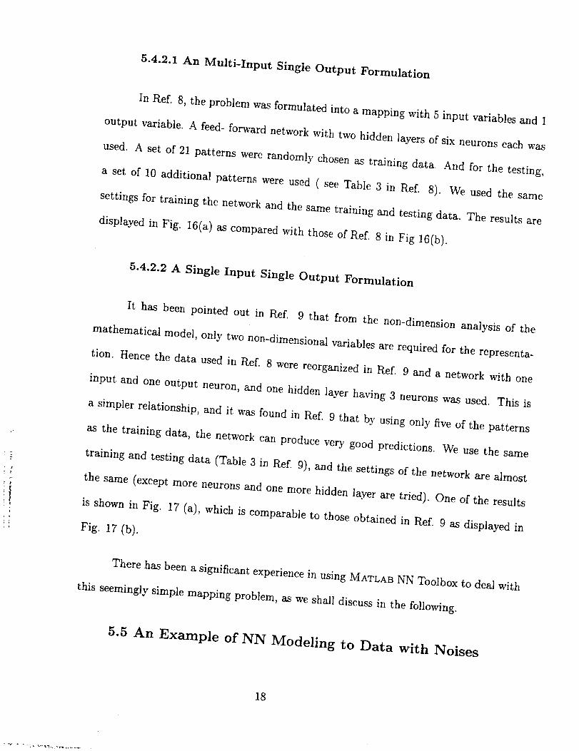
5.4.2.1 An Multi-Input Single Output Formulation

In Ref. 8, the problem was formulated into a mapping with 5 input variables and 1

output variable. A feed- forward network with two hidden layers of six neurons each was

used. A set of 21 patterns were randomly chosen as training data. And for the testing,

a set of 10 additional patterns were used ( see Table 3 in Ref. 8). We used the same

settings for training the network and the same training and testing data. The results are

displayed in Fig. 16(a) as compared with those of Ref. 8 in Fig 16(b).

:1: !

5.4.2.2 A Single Input Single Output Formulation

It has been pointed out in Ref. 9 that from the non-dimension analysis of the

mathematical model, only two non-dimensional variables are required for the representa-

tion. Hence the data used in Ref. 8 were reorganized in Ref. 9 and a network with one

input and one output neuron, and one hidden layer having 3 neurons was used. This is

a simpler relationship, and it was found in Ref. 9 that by using only five of the patterns

as the training data, the network can produce very good predictions. We use the same

training and testing data (Table 3 in Ref. 9), and the settings of the network are almost

the same (except more neurons and one more hidden layer are tried). One of the results

is shown in Fig. 17 (a), which is comparable to those obtained in l_ef. 9 as displayed in

Fig. 17 (b).

There has been a significant experience in using MATLAB NN Toolbox to deal with

this seemingly simple mapping problem, as we shall discuss in the following.

5.5 An Example of NN Modeling to Data with Noises

18

The exampleproblem usedin Ref. 11will besolvedhere by both feed-forward NN

and radial basis function (RBF) NN to show their respective abilities of modeling data

with noises.

A set of 51points sampleduniformly in the x-direction but with randomly chosen

noisesin the y-direction can be generatedby the MATLAB code as follows.

p=51;

x=O:. 02:1;

sigma=O. 15;

y=. 5 +.4 *sin(10 *x) + sigma * (. 5-raud(1,p ) ) ;

plot (x, y, 'c + ')

The true function, y(x)=.5+.4sin(10x), which will be generated with a more dense

set of points and plotted by dashed line, is sampled without noise.

pt=500;

xt=linspace(O, 1,pt) ;

yt=. 5 +.4 *sin(1 O'x) +sigma *(. 5-rand(1,p)) ;

hold on

plot(xt, yt, 'b- ')

The comparison of the training points with noises specified above, feed-forward

NN simulation with two hidden layers (1-20-20-1), and the true function is shown in Fig.

18(a). A similar comparison with a RBF NN simulation is shown in Fig. 18(b). We can

see that in both cases that the neural networks give reasonable and smooth simulation of

the true function even though the training data has noise.

19

Another set of training points is generatedwith noisesin both x- and y- direction.

This gives an evenworsesituation for the neural network to deal with.

p=51;

x=O:. 02:1;

sigmal=O. 01;

sigma2= O. 15;

x=x+sigmal *(. 5-rand(1,p));

y--.5+.4 *sin(l O*x) +sigma2 _(. 5-rand(1,p)) ;

plot(x,y, 'c+ ')

Comparison of the results in this case is shown in Fig. 19(a) through (d), where (a)

is about the results by a (1-20-20-1) Feed-Forward NN, (b) is about a RBF NN simulation,

(c) is a summation of the results in (a) and (b), and (d) is about the results by a (1-40-1)

FF NN trained with adaptive learning. Very good results are also obtained by all neural

network modeling. As in the first case, the RBF neural network gives the best results.

Shown in Fig. 20 is the result from the feed-forward NN with transfer function

combination Formulation I (see 6.3 in the following). In this case, it is difficult for

the training to converge, and back-propagation with adaptive learning (that means the

learning rate is adjusted in each epoch) has to be adopted. Moreover, the simulated result

curve is quite rough for both 1 and 2 hidden layer cases. We shall discuss this further in

6.3,

6. On Some Issues of Neural Network Modeling

6.1 About the Accuracy and Error Goal

2O

In a sense NN modeling is something similar to fitting a curve or interpolation. It

seems almost impossible that in the presence of a limited information set (the training

data) a NN can simulate the performance of a system under all possible input scenarios.

Quite often, both the training and the input data sets include all sorts of noises.

Generally, it is expected that the accuracy of a NN could be better in the case of

"interpolation" than in the case of "extrapolation" (for instance, see Figs. 14 and 15).

The error goal for the training of a NN has a direct impact on the training time and

some influence on the prediction accuracs;. It seems that since usually the data (whether

for training or for testing) is polluted by noise, a very small error goal would not be a good

strate_, for the training process. Besides a long training time or even failure to converge,

that sometimes may mean worse accuracy for the testing data outside the training set.

These have been clearly shown in Fig. 21. In Fig. 21(a) we can see that as a result

of very small error goal, the accuracy of testing is very poor despite a perfect training

accuracy, and in Fig. 21(b) and (c) through the choice of a moderate error goal, both

the testing and training accuracy are of the same order. For the case in Fig. 21(a) the

training time was about 5 times longer.

6.2 Normalization of the Training Data

When the Sigmoid or other transfer functions which squash the output in the range

[-1,1] are used, preparation of data is very important before modeling by NN and training.

For feed-forward neural networks, the input and output data must be normalized, that is

to say, they must be scaled to values less than 1. This is because the Sigmoid function

cannot give values larger than 1. Usually the largest value should be kept to a value that

21

is closeand tessthan 1, say0.98. If the original valuesof the input and output are much

lessthan 1, it should also be normalized and scaledto a value closeto 1.

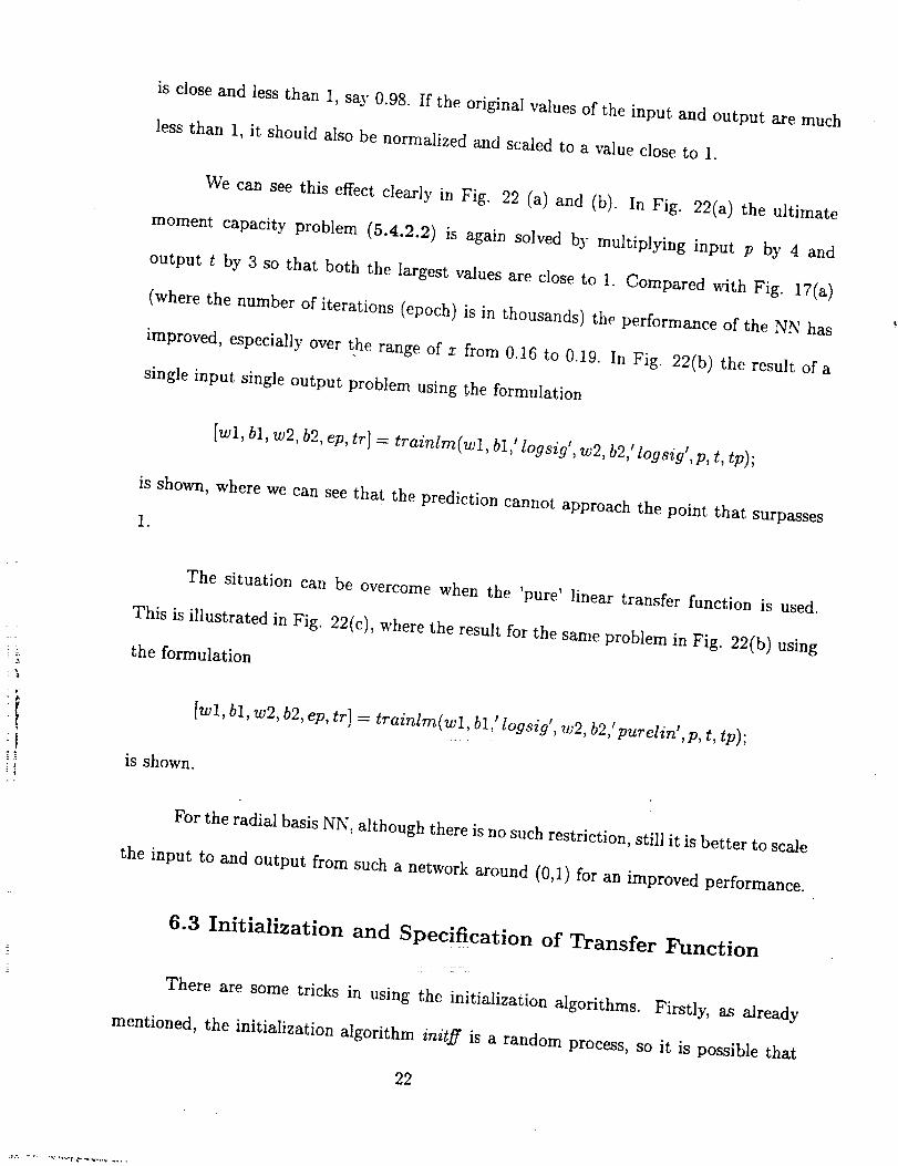
We can seethis effect clearly in Fig. 22 (a) and (b). In Fig. 22(a) the ultimate

moment capacity problem (5.4.2.2) is again solved by multiplying input p by 4 and

output t by 3 so that both the largest values are close to 1. Compared with Fig. 17(a)

(where the number of iterations (epoch) is in thousands) the performance of the NN has

improved, especially over the range of x from 0.16 to 0.19. In Fig. 22(b) the result of a

single input single output problem using the formulation

[wl, bl, w2, b2, ep, tr] = trainlm(wl, bl ,' logsig', w2, b2,' logsig', p, t, tp);

is shown, where we can see that the prediction cannot approach the point that surpasses

1.

The situation can be overcome when the 'pure' linear transfer function is used.

This is illustrated in Fig. 22(c), where the result for the same problem in Fig. 22(b) using

the formulation

[wl, bl, w2, b2, ep, tr] - trainlm(wl, bl, f logsig r, w2, b2/ purelin',p, t, tp);

is shown.

For the radial basis NN, although there is no such restriction, still it is better to scale

the input to and output from such a network around (0,1) for an improved performance.

6.3 Initialization and Specification of Transfer Function

There are some tricks in using the initialization algorithms. Firstly, as already

mentioned, the initialization algorithm initff is a random process, so it is possible that

22

training histories of a given problem may be quite different, with one showing a quick

convergence and the other needing thousands of extra iterations.

Secondly, the specification of the transfer function involved in initff and trainbp

has very large influences on the training history and the performance of the network. It

has been found that there are only two combinations of initff and trainbp that are feasible

in practice, as shown below:

Formulation I:

[w I , b 1, w2, b2, w3, b3]=init ff (p , n l , 'logsig ', n2, 'logsig ', t, 'logsig ');

[wl, b1, w2, b2, w3, b3, ep, tr]=trainbp (wl, b i, 'logsig ', w2, b2, 'logsig ', w3, b3, 'logsig ',p, t, tp);

Formulation II:

[w l , b 1, w2, b2, w3, b3]-init ff (p, nl , 'tansig ', n2, 'tansig ', t, 'tansig ');

[wl,b l,wg, b2,w3,b3,ep,tr]=trainbp(wl,b l, 'logsi9 ',w2,b2, 'logsi9 ', vo3,b$, 7ogsig',p,t, tp) ;

Formulation I usually makes the training process oscillate (the error-epoch line

quite rough) but approach the error goal more directly while the error-epoch line of

Formulation II is usually quite smooth but at the later part of training the error decreases

very slowly. See Figs. 4(b), 5(b) (Formulation//), and Fig. 3(a), 3(b) (Formulation I)

As to the performance of a NN, although Formulation I can predict the output in

the training data set quite well, it sometimes gives very poor testing results outside the

training data. See Fig. 23 and Fig. 13 (a) and (b). Further, from Fig. 18 to 20, we can

see while Formulation II gives quite robust and smooth performance Formulation I, in

contrast, gives unstable and rough predictions when the training data includes noise.

23

So we prefer Formulation II.

!

6.4 NN Structural Problem

The number of the hidden lavers and the number of neurons in each layer determine

the freedom or dimension of a NN. Generally speaking, more hidden layers and more

neurons in the layers mean a larger flexibility of the NN, and accordingly smaller error

goal can be specified.

The relation between the training time and the numbers of hidden layers and

neurons is a complicated one. A more complex NN (with more hidden layers and neurons)

certainly needs more execution time in each training iteration. But a network with more

layers or neurons may need less iterations for training to reach the desired error goal.

From Fig. 24 (a) through (h), we can say the adequate degree of freedom of a NN

(total number of neurons) is about the same order of the number of the training data sets.

More hidden layers and neurons not only increase the training effort, but sometimes also

give poor performance for the network.

7. Cross-Validation Algorithms and Some Obser-

vations

Cross-validation is a standard tool in statistics (Ref. 1). This technique can be

used to optimize neural network structural parameters, i.e. numbers of hidden layers and

neurons of each hidden layer etc. It can also be utilized to determine the proper training

epoch in order to avoid over-training, the case that usually occurs when the number of

training iteration is too high, with the symptom that errors for the training data approach

24

zero while those for the testing data increaseexcessively.

When a network is being trained using the cross-validation technique, the training

data is divided into two subsets,one subset being used for training of the network, the

other being used for validation (i.e. testing). The validation subset is typically 10 to 20

percent of the training set.

For the caseof single output, the error can be defined as the following combined

erTOr

= 1 s.) 2+_r Q- Us i=l i=I

t/2

where n_ and n_ are numbers of data sets in the training and testing subset respectively, tr

and t, are the target value for the training and testing subset, and st and ss are the values

predicted by the network for the training and testing subset. Other two error measures

are:

and

Et a -'-"

1 n, )i=l

1 n_ )i=l

1/2

i/2

are also of interest and so is the error ratio Et_/Et_.

MATLAB algorithms cvtrain, cvtrainl are available to train Feed-forward NN using

cross-validation. They are invoked in the following format

25

[wl , b l, w2, b2, w3, b3]= cvtrain (nI, n2,ic, dn, ran,p, t);

or

[wl, b 1, w2, b2, w3, b3]=cvtrain I (n 1, n2,ic, dn, mn,pr, tr, ps, ts);

where the training is accomplished by invoking trainbp or trainbpa, and descriptions of

the parameters can be found in their help message (see Appendix:. The only difference

between cvtrain and cvtrainl is that in the former the testing subset is determined in the

alogorithm in a random manner and takes about 20 percent of the training set, while in

the latter they are provided beforehand as pr, tr, ps, ts.

Several calculations have been carried out for two problems. The first problem is

the example problem used in 5.5, now with 21 points as training subset and 20 points as

testing subset, and the noise level still being at sigma = 0.15. The second is that in the

ultimate moment capacity problem (5.4.2.1), with the 21 sets of original training data

as training subset, and the 10 sets of testing data as testing subset. 'Feed-forward neural

networks with different configurations are used and some of the results are displayed in

Figs. 25 through 30. It should be noted that for the first problem since there exists a

real function, we can have two kinds of errors, one based on the noise polluted training

set, another based on points on the real function curve. Since what' we want to model is

the exact mapping in terms of the real function, and in practical problems this mapping

is usually nowhere to be found, the error based on real function should be paid more

attention.

Hereafter we look through the results, and some conclusions can be drawn, which

are true at least for the specific problems.

26

4

• There indeed exists an optimum epoch or range of epoch where the

combined error tends to be minimum, as can be seen clearly in Figs.

25(a), 26(a), 27(a) and 30(a), and partly in Figs. 28(a) and 29(a). The

optimum epoch for the error based on the real function is less than

that for the error based on the training data, the former being about

one half of the latter. The optimum epoch number decreases as the

network complexity increases.

• As number of the training epoch ir_creases_ the error on the training

subset, Eta, tends to decrease indefinitely and approaches zero, pro-

vided the network neuron number is large enough, as shown in Fig.

26(c), 27(c), 29(c), and 30(5). This results in the ratio Eta/Err based

on training data to increase drastically, as in Fig. 26(b), 27(b), and

29(b). But the ratio Ets/Et,. based on the real function is always in

the vicinty of 1.0 and very stable (see Fig. 25(b) through 29(b)). The

latter is expected since both Ets and Et_ here represent the average

difference between the network generalization and the real function.

• As to the problem of network complexity, at least for the choices having

been made, it seems that the best performance is given by a network

having about the same number of neurons as that of the training data

sets, a fact mentioned earlier. This observation is based on the assump-

tion that the real mapping is smooth and is unaffected by the noise in

the training and testing data.

• Cross-validation technique can be used to investigate a lot of problems

in NN training. But it is time-consuming and not mature enough to

27

be incorporated into a routine training process. A tentative standard

for stop to avoid over-training can be Ets/Etr=2 and Epoch>ran (a

minimum training number). But this strategy is not so successful (for

instance, it is not clear how to determine mn).

• Over-training is not so serious a problem as it seems to be. At least

beyond the optimum epoch the combined error only increases slowly.

As to the error ratio of testing over training, it is almost a constant (1.0)

if it is based on the real mapping and if the training and testing data

are uniformly noise-polluted. This means that training epoch should

be high enough. Under-training is worse than over-training and should

be avoided.

• From the figures it can be seen that for the example problem the train-

ing of network is locally unstable with one hidden layer while not with

two hidden layers. From Fig. 30(a) and some other results not included

here, we can see the situation for the ultimate moment capacity prob-

lem in 5.4.2.1 is the same. Obviously, in some way networks with two

hidden layers are superior to those with only one (Ref. 1).

• If a testing data is incorporated into a cross-validation process to train

a network, it contributes (at least indirectly) to the training and loses

its status as independent testing data.

8. Methods of Obtaining Continuum Models

A lot of methods have been used to develop continuum models to represent corn-

28

=

J

plex structures. Many of these methods involve the determination of the appropriate

relationships between the geometric and material properties of the original structure and

its continuum models. An important observation is that the continuum model is not

unique, and determining the continuum model for a given complex structure is inherently

ill-posed therefore diverse approaches can be used. This can be clearly shown in the

following example of determining continuum models for a lattice structure.

The single-bay double-laced lattice structure shown in Fig. 31 has been studied

in l_ef. 12, 13 and 14 with different approaches to the continuum modeling. This lat-

tice structure with repeating cells can be modeled by a continuum beam if the beam's

properties is properly provided.

Noor et al's method include the follwing steps (Ref. 12): (1)introducing assump-

tions regarding the variation of the displacements and temperature in the plane of the

cross section for the beamlike lattice, (2)expressing the strains in the individual elements

in terms of the strain components in the assumed coordinate directions, (3)expanding each

of the strain components in a Taylor series, and (4)summing up the thermoelastic strain

energy of the repeating elements which then gives the thermoelastic and dynamic coef-

ficients for the beam model in terms of material properties and geometry of the original

lattice structure.

In Sun et al (Ref. 13), the properties of the continuum model is obtained respectively

by relating the deformation of the repeating cell to different load settings under specified

boundary conditions. For example, the shear rigidity GA is obtained by performing a

numerical shear test in which a unit shear force is applied at one end of the repeating cell

and the corresponding shear deformation is calculated by using a finite element program.

The mass and rotatory inertia are calculated with a averaging procedure.

29

Lee put forward a method that he thought to be more straightforward (Ref. 14).

He used an extended Timishenko beam to model the equivalent continuum beam. By

expressingthe total strain and kinetic energ_of the repeating cell in terms of the dis-

placement vector at both ends of the continuum model, and equating them to those

obtained through the extendedTimishenko beam theory, he got a group of relations. The

number of theserelations, 2N(1÷2N), where N is the degree of freedom of the contnuum

model, is usually larger than that of the equivalent continuum beam properties to be

determined. Lee then introduced a procedure in which the stiffness and mass matrices for

both the lattice cell and the continuum model are reduced and so is the number of rela-

tions. Yet how to reduce the number of relations to be equal to the number of unkowns

seems depend on tuck.

All the above three methods give close results for the continuum model properties,

and the continuum models also generate promising results for the lattice structure.

9. An Example of NN

Models

Modeling of Continuum

Emphasizing the application of NN, we choose an approach similar to that in Ref.

13, that is, to derive the properties of the beam by investigating the force-deformation

relationships of the repeating cell in certain boundary conditions. The approach is illus-

trated in Figs. 32 (a), (b) and (c), where the beam's axial rigidity EA, bending rigidity

EI, and shearing ridigity GA are calculated respectively by using the results of finite

element analysis of the repeating cell in different load conditions. Concerning the finite

element analysis of 3-D lattice structures one can consult l_ef. 15.

There are five parameters of the repeating cell for the lattice structure in Fig.

3O

r

i

!1

i

!

31 that can be varied, the longitudinal bar length Lc, the batten length Lg, and the

longitudinal, batten and diagonal bar area, Ac, Ag and Ad. Generally, a function with

more variables will be more complex and it will be more difficult for a neural network

to simulate its performance. A NN with more input variables needs much more training

data since in the training data each variable should vary separately. As can be shown in

the following, this kind of "coarse" training data pose an obstacle to most of the training

algorithms.

Three scenarios were investigated, with the number of input variables set to be 2,

3 and 4 respectively.

9.1 Neural Network with 2 Input Variables

The input variables are Lc and Ac. The number of training data sets is 400=20x20.

The number of testing data, most of which are located at centers among the training data

mesh, is also 400=20x20. Part of the results, about GA, is shown in Fig. 33. Simulations

on the testing data and the relative errors of a FF NN (2-10-1) trained with Levenberg-

Marquardt (trainlm) are shown in Figs. 33 (b) and (c). Results of a RBF NN doing the

same job are shown in Figs. 33 (d) and (e).

We could not say that FF is superior over RBF just because its testing accuracy

shown in Fig. 33 (c) is higher than RBF's shown in Fig. 33 (e). We can adjust the

training criterion to change a RBF NN's behavior and it should be noted that what is

shown in Figs. 33 (d) and (e) are not RBF NN's best performances.

9.2 Neural Network with 3 Input Variables

31

The input variables were chosenas Lc, Ac and Ad. The number of training data

sets is 343=7xTx7. For this case, the effectiveness of different training algorithms can be

seen clearly in Fig. 34. When ordinary back-propagation training algorithm, i.e. trainbp

is used, it is very hard to train the NN to the error level of 10 -1, as shown in Fig. 34 (a).

When the adaptive learning technique is included, an improvement can be made, but it is

still hard to reach the 10 -_ error level, as can be seen in Fig. 34 (b). Now if the algorithm

with Levenberg-Marquardt (trainlm) is used, it is quite easy to push the training error

level to the order of 10 -4 .

The improvement by trainlm is really amazing. All the training algorithms carry

out an optimization process. While trainbp uses steepest-descent method with constant

step size, trainbpa accelerates the process by adjusting the step size. On the other hand,

trainlm adopts a kind of modified Newton's Methods, which adjusts both the searching

direction and the step size. Concerning the optimization methods one can consult Ref.

16.

Samples of the NN simulation results are given in Table 3, where the desired values

and values obtained by Noor et al (Ref. 12) and Lee (Ref. 14) are also presented.

9.3 Neural Network with 4 Input Variables

The input variables were chosen as Lc, Ac , Ag and Ad. The number of training

data sets is 625=5x5x5x5. For this case only trainlm could trait a FF NN that could

give resonable results. Samples of the NN simulation results are given in Table 4.

32

10. References

[1]L. P. J. Veelenturf, Analysis and Application o/Artificial Neural Networks, Pren-

tice Hall, 1995

[2]S. Haykin, Neural Networks: A Comprehensive Foundation, Macmillan College

Publishing Company, 1994

[3]G. Cybenko, "Neural Networks in Computational Science and Engineering",

IEEE Computational Science and Engineering, Spring 1996

[4]K. Hornik, M. Stinchcombe and H. White, "Multilayer Feedforward Networks

are Universal Approximators", Neural Networks, Vol. 2, 359-366, 1989

[5]E. J. Hartman, J. D. Keeler and J. M. Kowaski, "Layered Neural Networks

with Gaussian Hidden Units as Universal Approximators",Neural Computation, Vol. 2,

210-215, 1990

[6]L. C. Rabelo, V. Shastri, E. Onyejekwe, and J. Vila, "Using Neural Networks

and Abductive Modeling for Device-Independent Color Correction", Scientific Computing

and Automation, May 1996

[7]K. M. Abdalla, G. E. Stavroulakis, "A Backpropagation Neural Network Model

for Semi-rigid Steel Connections", Microcomputers in Civil Engineering, 10 (1995) 77-87

[8]R. D. Vanluchene, R. Sun, "Neural Network in Structural Engineering", Micro-

computers in Civil Engineering, 5 (1990) 207-215

[9]D. J. Gunaratnam, J. S. Gero, "Effect of Representation on the Performance

of Neural Networks in Structural Engineering Applications", Microcomputers in Civil

33

Engineering, 9 (1994) 97-108

[10]S. L Lipson, "Single-Angle and Single-Plate Beam Framing Connections", Pro-

ceedings of Canadian Structure Engineering Conference, Toronto, Ontario 1968, 141-162

Ill]Mark J. L. Orr, "MATLAB Routines for Subset Selection and Ridge Regression

in Linear Neural Networks", Center for Cognitive Science Edinburg University, Scotland,

UK.

Accessible at http ://www. cns. ed. ac. uk/people /mark/rb f .html

[12]A. K. Noor, M. S. Anderson and W. H. Greene, "Continuum Models for Beam-

and Platelike Lattice Structures", AIAA Journal, Vol. 16, No. 12, Dec. 1978, pp. 1219-

1228

[13]C. T. Sun, B. J. Kim and J. L. Bogdanoff, "On the Derivation of Equivalent

Simple Models for Beam- and Plate-Like Structures in Dynamic Analysis", AIAA Paper

81-0624, 1981, pp. 523-532

[14]U. Lee, "Dynamic Continuum Modeling of Beamlike Space Structures Using

Finite-Element Matrices", AIAA Journal, Vol. 28, No. 4, Apri. 1990, pp. 725-731

[15]C. T. F. Ross, Finite Element Methods in Structural Mechanics, Ellis Horwood

Ltd., 1985

[16]J.-S. R. Jang, C.-T. Sun and E. Mizutani, Neuro-Fuzzy and Soft Computing: A

Computational Approach to Learning and Machine Intelligence, Prentice Hall, Inc., 1997

34

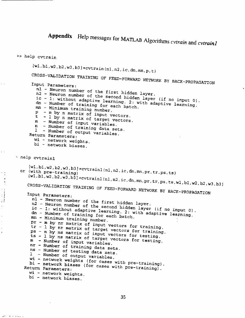
Appendix Help messages for MATLAB Algorithms cvtrain and cvtrainl

>> help cvtrain

[wl,bl,w2,b2,w3,b3]=cvtrain(nl,n2,ic,dn,mn,p,t)

CROSS-VALIDATION TRAINING OF FEED-FORWARD NETWORK BY BACK-PROPAGATION

Input Parameters:

nl - Neuron number of the first hidden layer.

n2 - Neuron number of the second hidden layer (if no input 0).

ic - i: without adaptive learning. 2: with adaptive learning.

cln - Number of training for each batch.

mn - Minimum training number.

p - m by n matrix of input vectors.

t - 1 by n matrix of target vectors.

m - Number of input variables.

n - Number of training data sets.

1 - Number of output variables.

Return Parameters:

wi - network weights.

bi - network biases.

11

- help cvtrainl

[wl,bl,w2,b2,w3,b3]=cvtrainl(nl,n2,ic,dn,mn,pr,tr,ps,ts)

or (with pre-training)

[wl,bl,w2,b2,w3,b3]=cvtrainl(nl,n2,ic,dn,mn,pr,tr,ps,ts,wl,bl,w2,b2,w3,b3)

CROSS-VALIDATION TRAINING OF FEED-FORWARD NETWORK BY BACK-PROPAGATION

Input Paralneters:

nl - Neuron number of the first hidden layer.

n2 - Neuron number of the second hidden layer (if no input 0).

ic - i: without adaptive learning. 2: with adaptive learning.

dn - Number of training for each batch.

mn - Minimum training number.

pr - m by nr matrix of input vectors for training.

tr - 1 by nr matrix of target vectors for training.

ps - m by ns matrix of input vectors for testing.

ts - 1 by ns matrix of target vectors for testing.

m - Number of input variables.

nr - Number of training data sets.

ns - Number of testing data sets.

1 - Number of output variables.

wi - network weights (for cases with pre-training).

bi - network biases (for cases with pre-training).

Return Parameters:

wi - network weights.

bi - network biases.

35

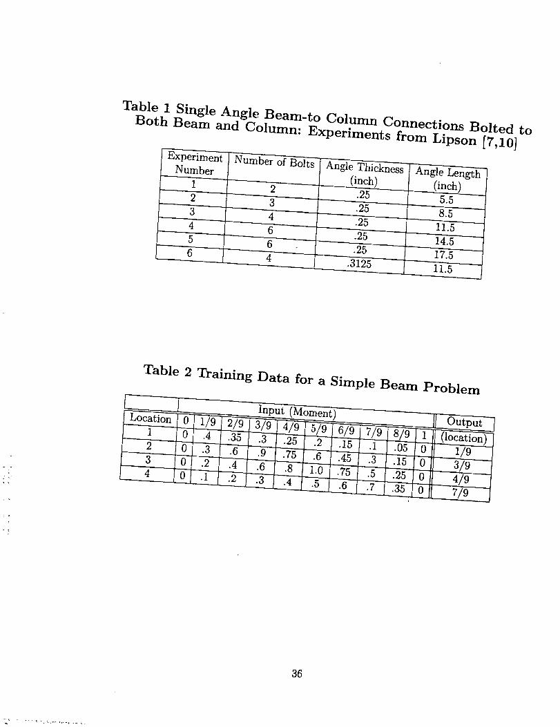
Table 1 Single Angle Beam-to Column Connections Bolted toBoth Beam and Column: Experiments from Lipson [7,10]

Experiment

Number

1

2

3

Number of Bolts

2

3

Angle Thickness

(inch)

Angle Length

L. .. (inch,).25 5.5

.25 8.5i - - -

.25 11.5

4 6 .25 14.5

5 6...... .25- 17.56 4 .3125 11.5

Table 2 Training Data for a Simple Beam Problem

Input Moment) Output

Location 6' "1/9 2/91, 3/91 4/9 5/9 6/9 7/9 8!9' i (location)

1 0 .4 .35 .3i.25 .2 .15 .1 .05 0 2/92 0 .3 ".6 .9 .75 .6 .4:5 .3 .i5 0 3/9

3 '0 .2 .'4 ".6 .8 _[.0 .35" .5 .25 0 4/9

4 0 -.1 .2 .3 .4 .5 .6 .7 .35 0 7/9

36

t_

C_o

oo

_o

0o

c_

oo _r_

t_ L_

O0 _

i- I

_....

o°

t_

oo_t_

X_

X _

_×

C_

luQe

?_-

C_

I,Wbe

r_

37

_...Jo

b..l°

w _

_D

rw_c_

× II

_×

Jt_

& JI

IfC_

×

IC31

_J

ImJo

_ _°

c_

38

r _ _..... t ._ .....

0©

-1 0

: = © C 1

n

input layer hidden layers output layer

Fig. l(a) Feed-Forward Multi-Layer Neural Network

1

0.8

0.6

0.4

0.2

0

-0.2

-0.4

-0.6

-0.8

-1-10

,,, t

angent

Linear

.I. | o J / i

0 2 4 6 8

r

10

Fig. l(b) Transfer Functions

39

number ofneurons- /'/l

/_/2 i/3

input hidden outputlayer layer layer

Fig. 2 Radial Basis Function Neural Network

40

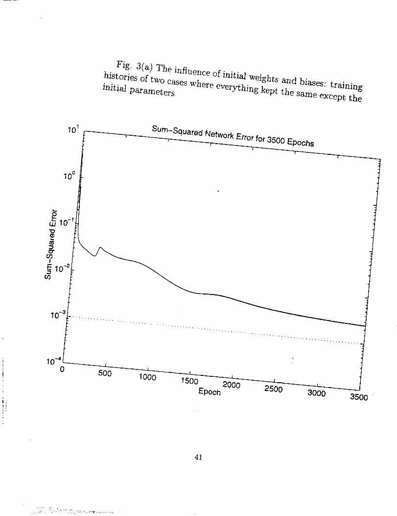
Fig. 3(a) The influence of initial weights and biases: training

histories of two cases where everything kept the same except theinitial parameters

Sum-Squared Network Error for 3500 Epochs

100

10 -3

5001000

1500 2000Epoch 2500 3000

3500

41

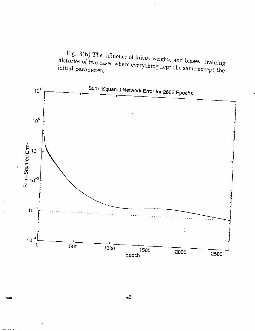
Fig. 3(b) The influence of initial weights and biases: training

histories of two cases where everything kept the same except theinitial parameters

Sum-Squared Network Error for 2666 Epochs

100

10 .3

10 -4

0I

500 1000J.

1500Epoch

I

2000 2500

42

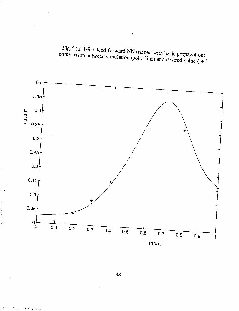
Fig.4 (a) 1-9-1 feed-forward NN trained with back-propagation:

comparison between simulation (solid line) and desired value ('+')

0.45

-.I

4.-,1

0 0.35

0.25

0.15

0.05

00

0.7 0.8 0.9

input

43

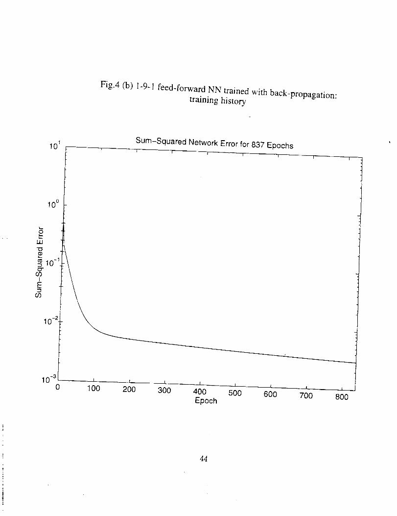
Fig.4 (b) 1-9-1 feed-forward NN trained with back-propagation:

training history

101

100

UJ"0

= 10 -I

09I

E

10 -2.

10 -30

I

100 200

Sum-Squared Network Error for 837 EpochsI

I | I I '

1. I I 1

300 400 500 600Epoch

I I

700 800

44

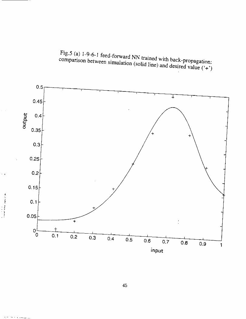
Fig.5 (a) 1-9-6-I feed-forward NN trained with back-propagation:

comparison between simulation (solid line) and desired value ('+')

0.45

0.25

0.15

0.05

00

+

+

O.6 0.7 0.8 0.9

input

45

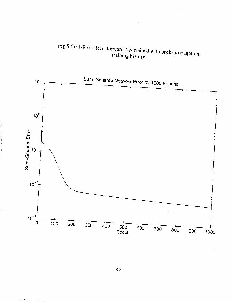
Fig.5 (b) 1-9-6-1 feed-forward NN trained with back-propagation:training history

Sum-Squared Network Error for 1000 Epochs

100

100 200 300400 500 600

Epoch700 800 900 1000

46

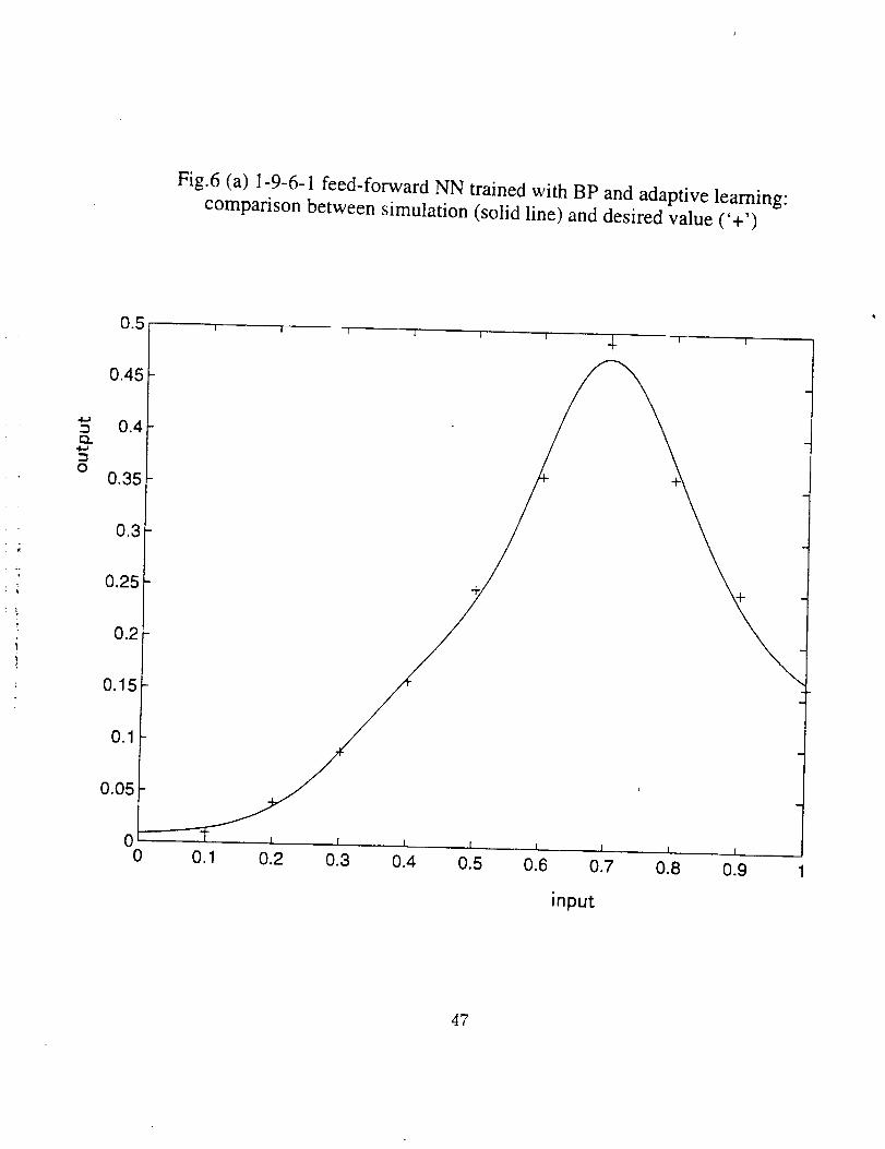
Fig.6 (a) 1-9-6-1 feed-forward NN trained with BP and adaptive learning:

comparison between simulation (solid line) and desired value ('+')

0,45

= 0.4

O0.35

0.3

0.25

0.2

0.15

0.1

0.05

00

, [ I I i I 1 I I

0,1 0.2 0.3 0.4 0.5 0.6 0.7 0.8 0.9

input

47

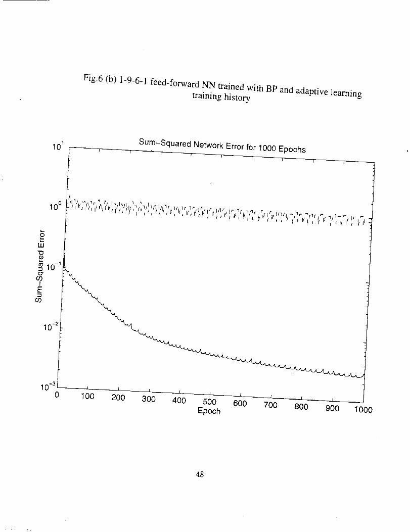
Fig.6 (b) 1-9-6-l feed-forward NN trained with BP and adaptive learning

training history

101

100

LB

"Z3,m

10 -_

03I

E

03

10 -2

Sum-Squared Network Error for 1000 Epochs1 I 1 t I I I I I

10 -3 , _ _ i 1 i _ _ _. . t0 1O0 200 300 400 500 600 700 800 900 1000

Epoch

48

0.8

0.6

0.4

0 80.40.40.6

0.8 0.2

" 1 0x Y

Fig. 7 The mapping of z -- 2(1 + sin(4xy_))

49

0.8

W0.6

0.4

0.2

o.__ _;o., -0.8 0.2

1 0x Y

Fig. 8(a) Simulated mapping by a 2-10-1 NN trained by llxll uniformly

distributed data

°°'1

-0.005

o, -.._ _oo --

1 0 yx

Fig. 8(b) The relative error compared to the exact mapping (Fig. 7)

5O

1.

0.8

0.6

0.4

0.2

o.__ _/._., _.°0.8 O.2

I 0

Fig. 9(a) Simulated mapping by a 2-10-] NN trained by 121 sets of

randomly distributed data

0.151

0"1t0.05

0-'

-0.050

O.2 1

0.6

0.6 O.6

1 0

Fig. 9(b) The relative error compared to the exact mapping (Fig. 7)

51

0.8.

0.6.

0.4.

0.2,

O_

0.4

• 0.4

0.8 0.2

1 0

Fig.

10(a) Simulated mapping by a 2-10-1 NN trained by 24 sets of

randomly distributed data

0.3,

0.2 •

0.1

O.

-0.1,

0

,41

1 0

Fig. 10(b) The relative error compared to the exact mapping (Fig. 7)

52

1.2Relative Error as a function of n/n0

0.8

> 0.6

-$rr

0.4

0.2

O o: Relative Error with randomly distributed training data

o" Averaged Relative Error with randomly distributed training data

00

--: Averaged Relative Error with uniformlydistributed training data

-.-: y=0.07/x8

O

o \0 o_'_\ • 0 0

0

8-"_ o o

o O

J _ " -- I

0.2 0.4 0.6 0.8 1 1.2n/n0

Fig. 11 The relative error as a function of 77= ,_o

53

°, .'!

i ...... :

, !I

, I

I

I

I

I i

...... -......... i "1

........... ,_... ........i .............

I

I

_ J

Fig.12 Single Angle Beam-to Column Connection

54

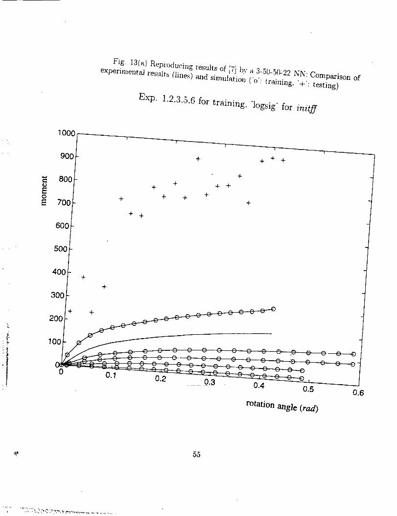
Fig. 13(a) Reproducing results of [71 by a 3-50-50-22 NN: Comparison of

experimental results (lines) aad simulation ('o': training. "+,: testing)

Exp. 1.2.3,,5.6 for training. "logsig" for initff

1000

E0E

9OO

80O

700

6O0

+

++

+ + + +

+ + + +

++ +

+

+

500

400

300

200

100

0

+

+ +

+

0.4 0.5

rotation angle (rad)

0.6

55

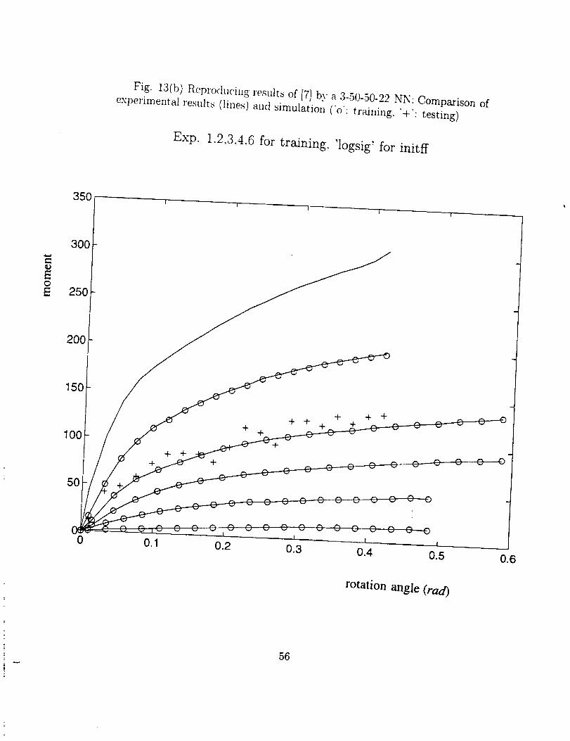
Fig. 13(b) Reproducing results of [7] by a 3-50-50-22 NN: Comparison of

experimental results (lines) and simulation ('o'- training. "+'. testing)

Exp. 1.2,3,4.6 for training, 'logsig' for initff

EO

E 250

200

150

100

5O

+ +

+ +

++

+ + ++ +

+ +

0 I I

0.4 0.5

rotation angle (tad)

0.6

56

Fig. 13(c) Reproducing results of [7] by a 3-50-50-22 NN: Comparison of

experimental results (|ines) and simulation ('o'- training. "+,: testing)

Exp. 1,2.3.5.6 for training. 'tansig' for initff

200

+ ++

150

IO0

5O

01

.J.

0.4 0.5

rotation angle (rad)

0.6

57

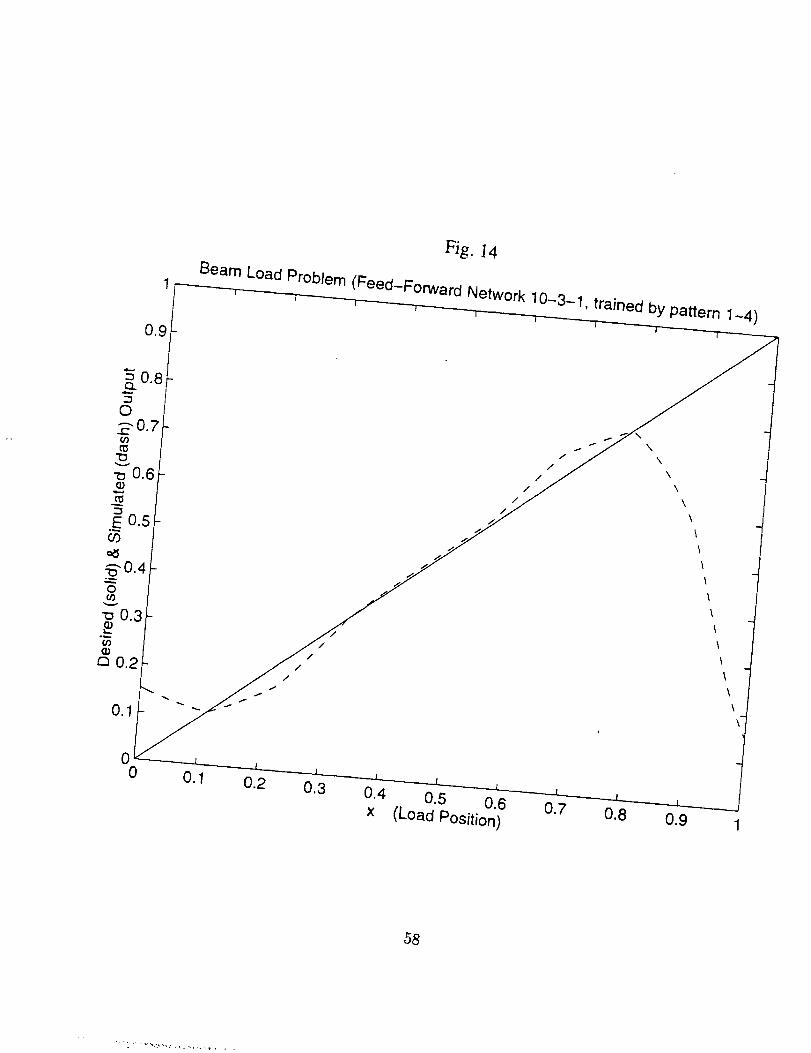
Fig. 14

Beam Load Problem (Feed-Forward Network 10-3-1, trained by pattern 1~4)

00

/

/

0.4 0.5 0.6

x ('Load Position)

/

/

\

\

\

\

\

58

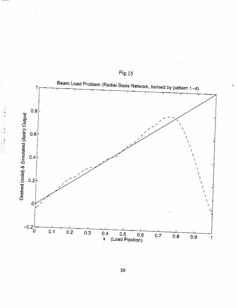
Fig.15

Beam Load Problem (Radial Basis Network, trained by pattern 1-4)

OA

r-

"O

'-IE

.m

O9

.i

Oo9

¢9

tm0

-0.2 f

0

/

I

0.1

/ \f

/ \

/ \/

l { { • I l I I

0.2 0.3 0.4 0.5 0.6 0.7 0.8 0.9x (Load Position)

\

\

\

\

\

\

\

\

\

\

\

\

\

\

\

1

59

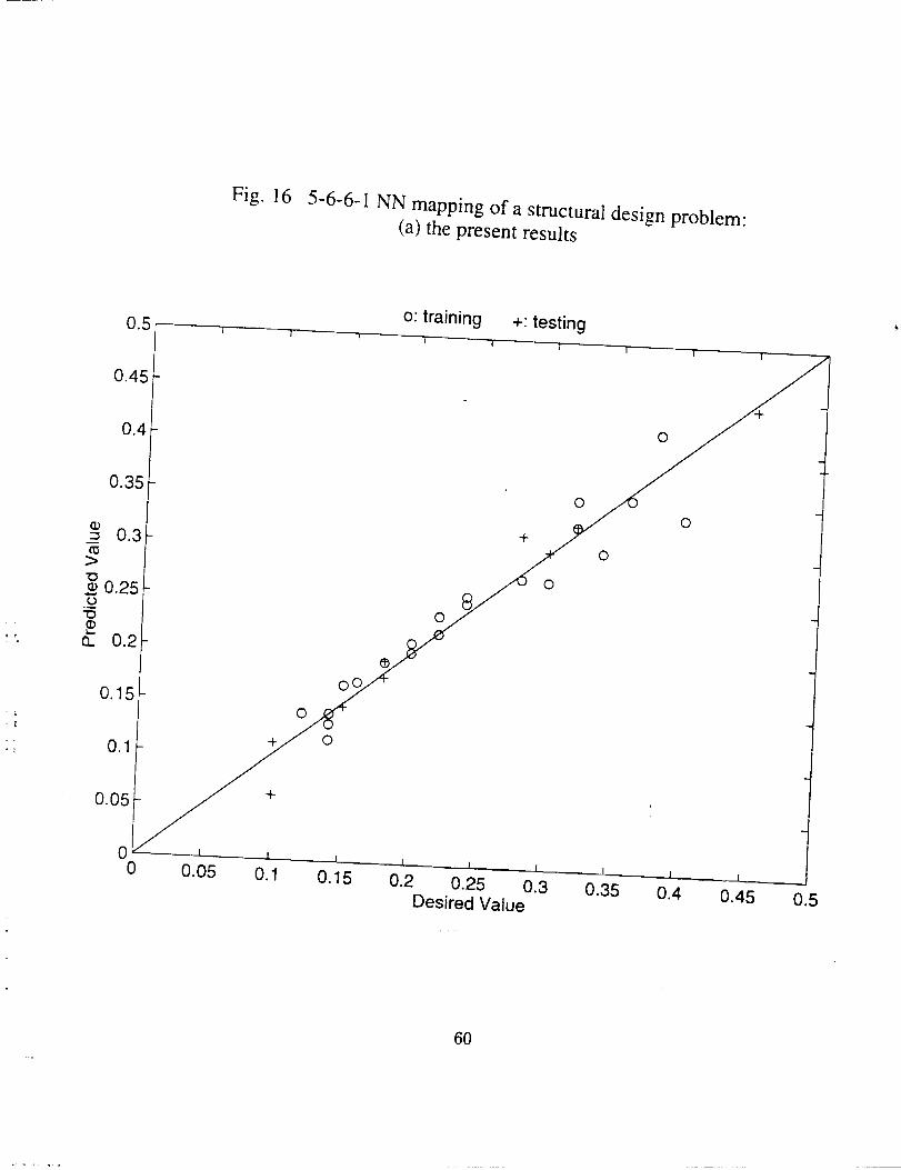
Fig. 16 5-6-6-1 NN mapping of a structural design problem:(a) the present results

o: training +: testing

0.45

O

0.35

O

©

O

O

O

0.15

+

O

©

O

0.05 +

00

0.05 0.1 0.15 I I

0.2 0.25 0.3 0.35 0.4Desired Value 0.45 0.5

60

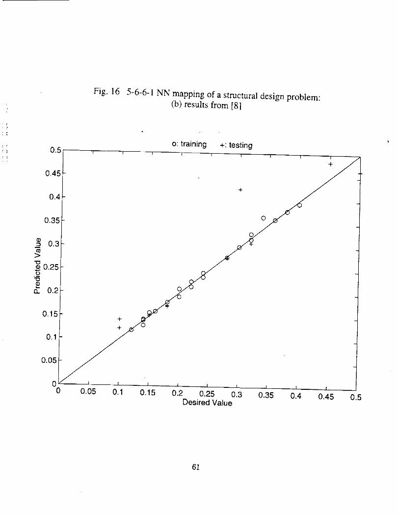
Fig. 165-6-6-l NN mapping of a structural design problem:

(b) results from [8]

0.45

I I I

o: training +: testingI I I

+

Jr

0.35 O

0.15Jr

Jr

0.05

0 I I

0 0.05 0.1 0.15I I I

0.2 O.25 0.3Desired Value

0.35 0.4 0.45 0.5

61

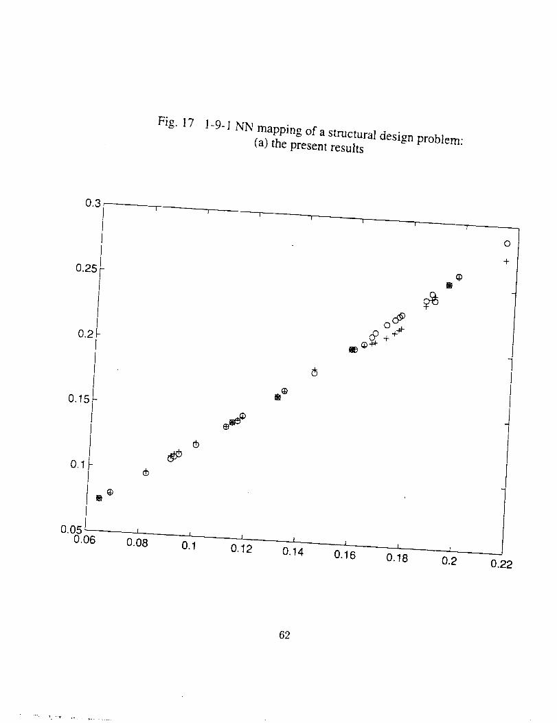
Fig. 17

1-9-1 NN mapping of a structural design problem:(a) the present results

0.25

0.2

0.15

0.1

@

0.050.06 0.08

(:b

0.12 0.14 0.16 0.18 0.2

0

+

0.22

62

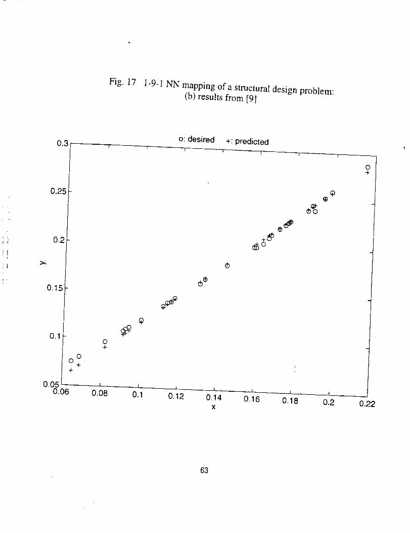
Fig. 17 1-9-1 NN mapping of a structural design problem:

(b) results from [9]

o: desired +: predicted

0.25

0.15

0

+

0.050.06

0+

0

+

I I

0.08 0.1 0.12I

0.14X

I

0.16I

0.18I

0.2 0.22

63

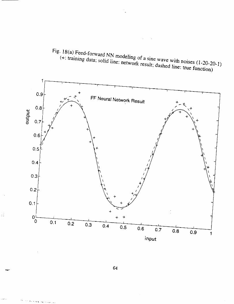
Fig. 18(a) Feed-forward NN modeling of a sine wave with noises (1-20-20-1)

(+: training data; solid line: network result; dashed line: true function)

I | | I | I 'l I '1

O

0.9

0.8

0.7

0.4

0.3

0.2

0.1

00

+

- _+ FF Neural Network Result +.-- +,,+"+_ \ - / \+

,+y-+_. /_,

// '\ /1 -,-'_

+t s ti +k+ ,l t,,

\, ,'/ \,

k ,,/ t-), ,q\,+ ,7'

x +

+

+ +

. 1 _ _. ! . _. 1 t. . I I 1 ! ,, I , ,,

0.1 0.2 0.3 0.4 0.5 0.6 0.7 0.8 0.9 1

input

64

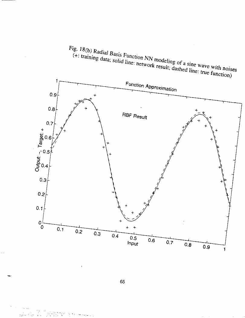
Fig. 18 (b) Radial Basis Function NN modeling of a sine wave with noises

(+: training data; solid line: network result; dashed line: true function)

0.9

0.B

0.7

+.

,-o.5!• •

Q.-" 0.4O

0.3

0.2

0.1

00

Function ,_pproximation| | I I I _ ] I 'l " "

+

2 + \RBF Result +(f,"' + 'k_\+

¢ ) ,i \\- ,/ \

*\ +,,/

'\;+/+

+ +

I , I I I I _ I I I , .

0.1 0.2 0.3 0.4 0.5 0.6 0.7 0.8 0.9Input

65

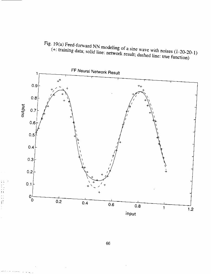
Fig. 19(a) Feed-forward NN modeling of a sine wave with noises (1-20-20-1)

(+: training data; solid line: network result; dashed line: true function)

FF Neural Network Result1

i ++0.9 i- +

_ 0.7

0.6

0.5

0.4

0.3 /"

0.2 + //

\ +

O"I +\_ //++

J" .L

0 0.2 0.4 0.6

++

+

+

4-

66

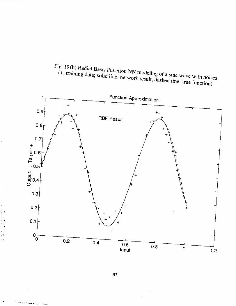
Fig. 19 (b) Radial Basis Function NN modeling of a sine wave with noises

(+: training data; solid line: network result; dashed line: true function)

- +++

RBF Result ++.

+

+

01

0 0.2 0.4

++

+

._L-L

0.6 0.8 ..LInput 1 1.2

67

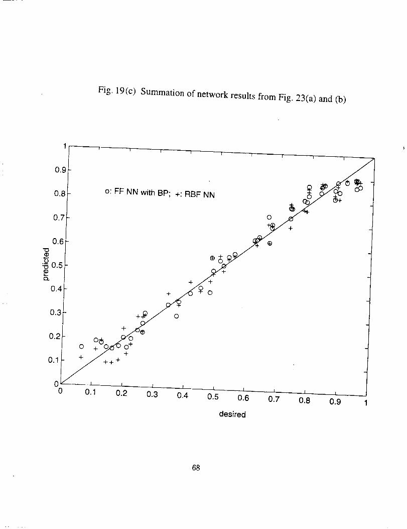
Fig. 19(c) Summation of network results from Fig. 23(a) and (b)

©

+

o: FF NN with BP; +: RBF NN

+

+ ©

O

00

desired

68

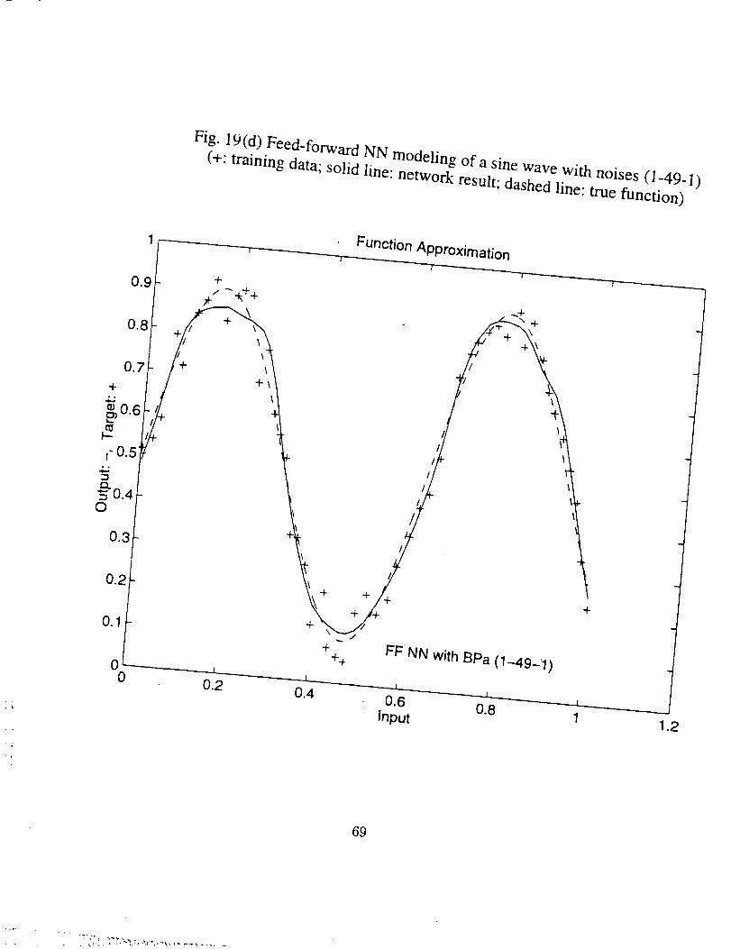
Fig. 19(d) Feed-forward NN modeling of a sine wave with noises (1-49-1)

(+: training data; solid line: network result; dashed line: true function)

0.7 +

+• ,

0.6

1"0.5. o

= 0.4O

0.1

00.2

+

J_

0.4

+

\

+

++

Function ApProximation

+

FF NN with BPa (1-49-'1)

-L

0.6Input 0.8

.L

1

t

69

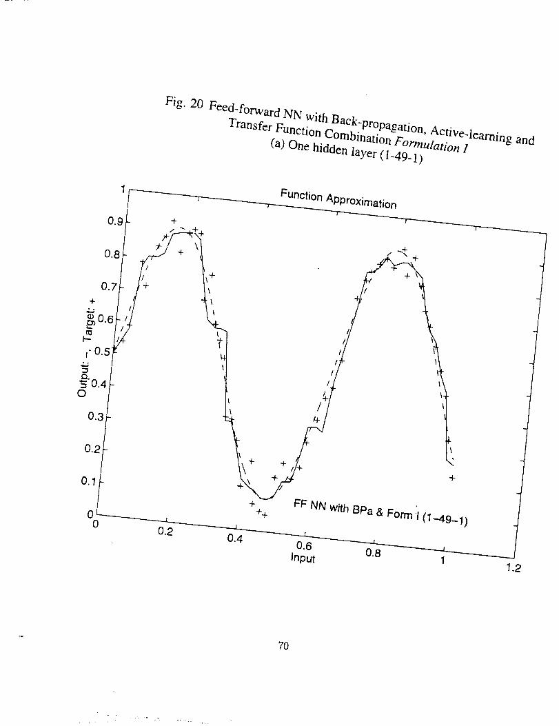
Fig. 20 Feed-forward NN with Back-propagation, Active-learning andTransfer Function Combination Formulation 1

(a) One hidden layer (1-49-1 )

Function ApProximation

+ +

+

+

++

+

+

/+

+

FF NN With BPa & Form '1(1-49-1)

M.

0.6 .LInput 0.8 _1

7O

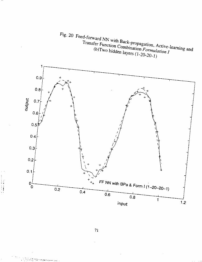
Fig. 20 Feed-forward NN with Back-propagation, Active-learning andTransfer FUnction Combination Formulation 1

(b)Two hidden layers (1-20_20_ 1)

00

+

+

+

+

++

3.

0.4

71

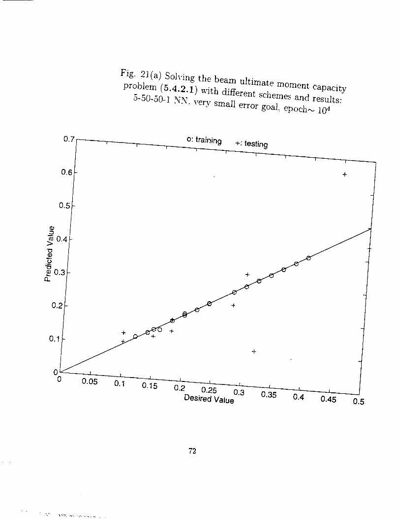
Fig. 2l(a) Solving the beam ultimate moment capacity

problem (5.4.2.1) with different schemes and results:

5-50-50-1 NN. very small error goal, epoch_ 104

° o

+

+

+ +

+

00 0.05

0.150.2 0.25 0.3

Desired Value0.35

0.45

72

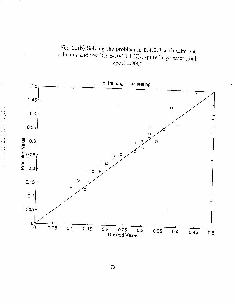
Fig. 21(b) Solving the problem in 5.4.2.1 with different

schemes and results: 5-10-10-1 NN. quite large error goal,epoch=2000

0.5

0.45

0.4

0.35

(D0.3

>

0.25.o

o.. 0.2

0.15

0.1

0.05

00

/"0.05 0.1

o: training +: testing

! I f I f I I

- 0 4"

0 0

o

l t I I I I

0.15 0.2 0.25 0.3 0.35 0.4Desired Value

0.45 0.5

73

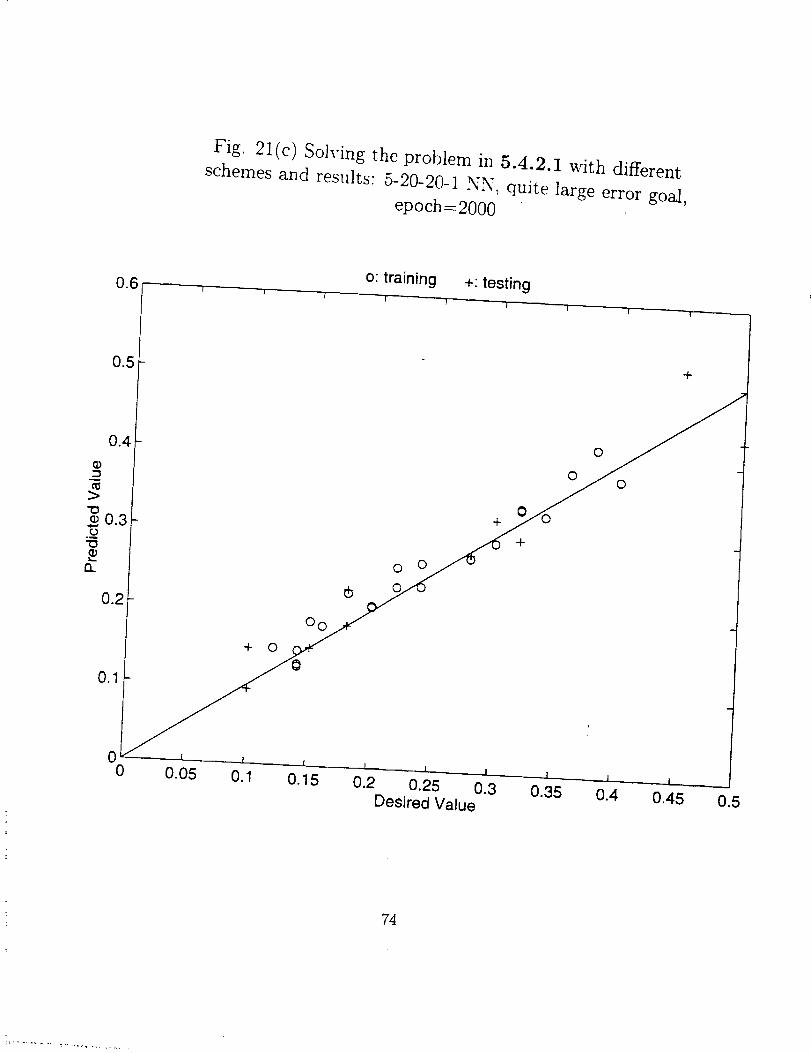
Fig. 21(c) Soh'ing the problem in 5.4.2.1 with different

schemes and results: 5-20-20-1 NN, quite large error goal,

epoch=2000

0.6o: training +: testing

t l I I 1 1 1 [ !

0.5

0.4

cD

>"0

0.3

D-

0.2

0.1

00

+ 0

cb

O0

0 0

+

I [ J I I

O.15 0.2 0.25 0.3 0.35Desired Value

+

0

0 0

1

0.4I

0,45

74

Fig.22(a) Normalization of input and output variables: the

problem in 5.4.2.2. 1-9-1, 4*p. 3*t. epoch=468

o: desired +: predicted *: training data

0

>.,

0.25

0.15

+

0.050.06 0.08 0.12 0.14

X0.16

0.18 0.2 0.22

75

1.4

I._

I

O,,q

0.4

0.2

4.

0.1 0,2 03 0.4 5 0.6 0.7 O.8 0

X

Fig. 22 (b) Normalization of input and output variables: 'logsig', 1-10-1,

training data t(.7) = 1.22 > 1, symbols: desired values, line: simulation

s

i

1

0.8

0,6

0.4

0,2

0

,. ,. , ,- , , ,, , ,, • • ..... ,

r

o:, 0:2 -o_ o:, 0:5 o:e o:, o:8 o:0X

Fig. 22 (c) Normalization of input and output variables: 'purelin I

76

i

i

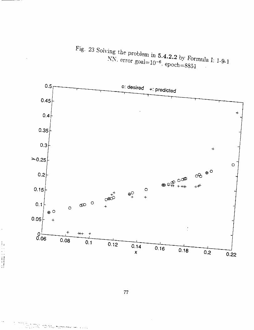
Fig.

23 Solving the problem in 5.4.2.2 by Formula I: 1-9-1NN. error goa]_lO_6 epoch=8851

0.5

0"45 t

0.4-

o: desired+: predicted

0.35

0.3

_'0.25

0.2

0.15

0.1

0.05 +

+

0_o

0+

0

0 4- -N-+ +

0.06

0,16 0.18x 0.2 0.22

77

-......

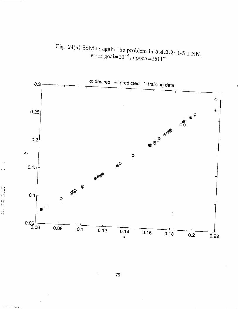
Fig.

24(a) Solving again the problem in 5.4.2.2:1-5-1 NN,

error goal= 10 -6, epoch = 15117

o: desired +: predicted *: training data

0

0.25

0.15

®

0.05O.O6 0.08

0.12 0.14X

0.160.18 0.2

+

0.22

78

Fig.24(b) Solving again the problem in 5.4.2.2:

error goal=lO-6, epoch=21551-6-1 NN,

O

0.25

0.15

0+

+

0.050.06

0.08 0.1 0.12 0.141

0.16 0.18 0.2 0.22

79

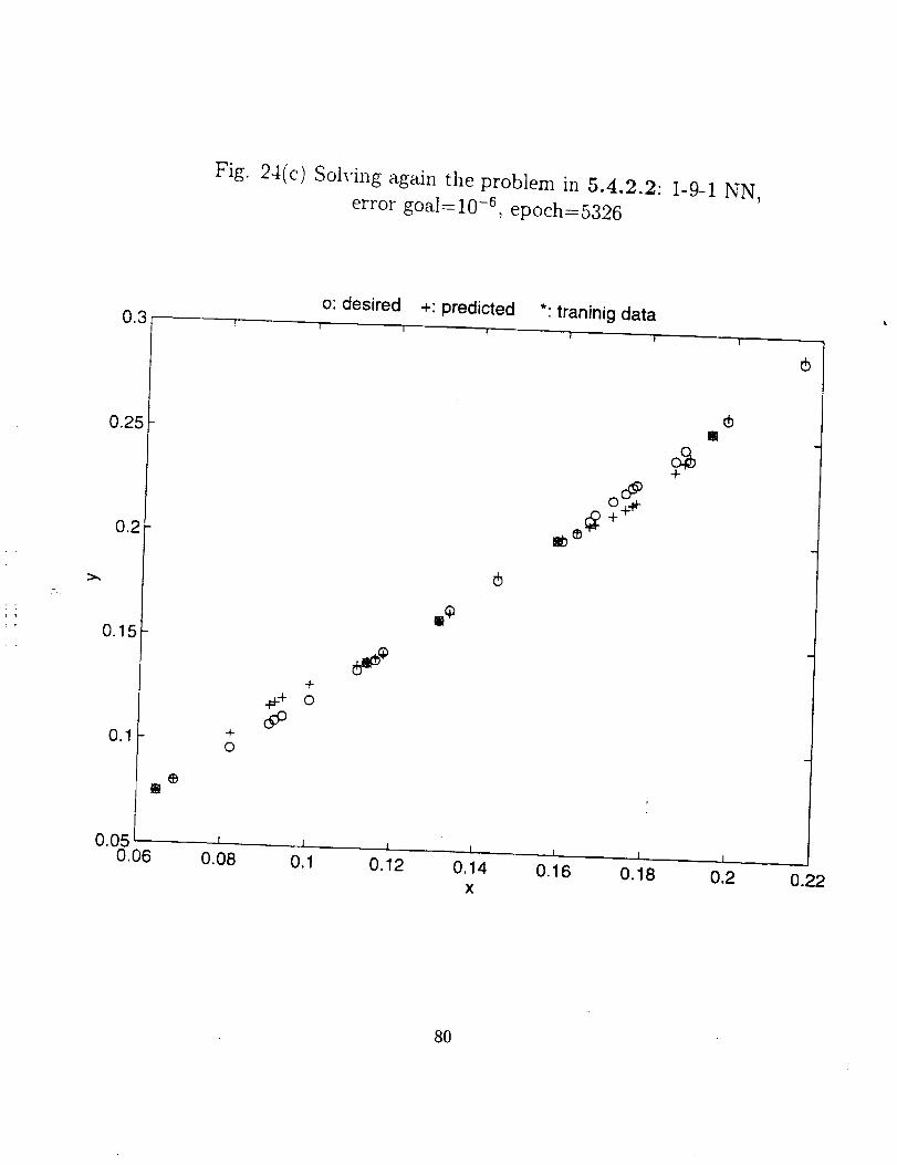
Fig.24(c) Soh'ing again the problem in 5.4.2.2:1-9-1 NN,

error goal=10-6, epoch=5326

03o: desired

r _T+: predicted *" traninig data

0.25

0.15

@

÷0

+

0

0.050.06 0.08

0.22

8O

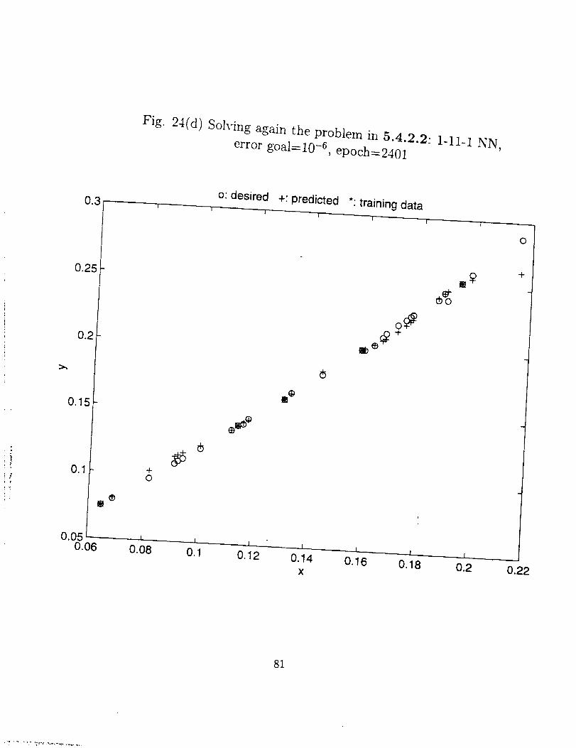
Fig.

24(d) Soh'ing again the problem in 5.4.2.2:1-11-1 NN,error goal=10-6, epoch=2401

o: desired +: predicted *: training data

0.25

0.15

0.1

®

0.050.06

+0

0.08 0.1 0.120.14 0.16 0.18 0.2

x

0

+

0.22

81

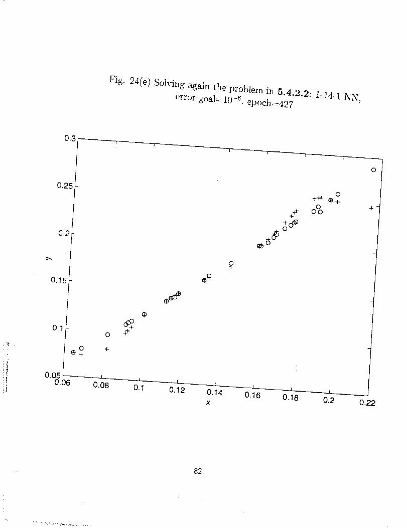
Fig. 24(e) Solving again the problem in 5.4.2.2:

error goal=10-6, epoch=4271-14-1 NN,

0.3

0.25

0.2

0

O+44 lit+

& +

0.15 • q_

O. . . • u. _o 0.2 0.22

82

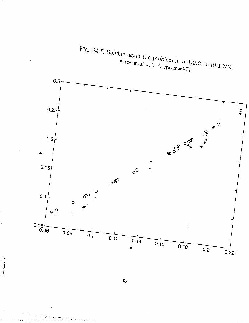
Fig. 24(f) Solving again the problem in 5.4.2.2:1-19-1 NN,

error goal=10 -6, epoch=971

0.3;

0.25

0.2

0.15

0.1

0_+

0.050.06

1 I ! ! | 1 I

0

+

0

+

0

+

i , I t , I I

0.08 0.1 0.12 0.14 0.16

×

ooo+

+

+

,I

0,18

+0

I

0.2

83

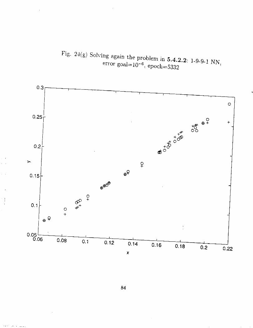
Fig.24(g) Soh-ing again the problem in 5.4.2.2:

error goal=lO-6 epoch=53321-9-9-1 NN,

O

0.25

0.15

©

+

0+

+-,-

+

0.050.06 0.08

I

0.1 0.12 0.14

X

0.16 0.18 0.2 0.22

84

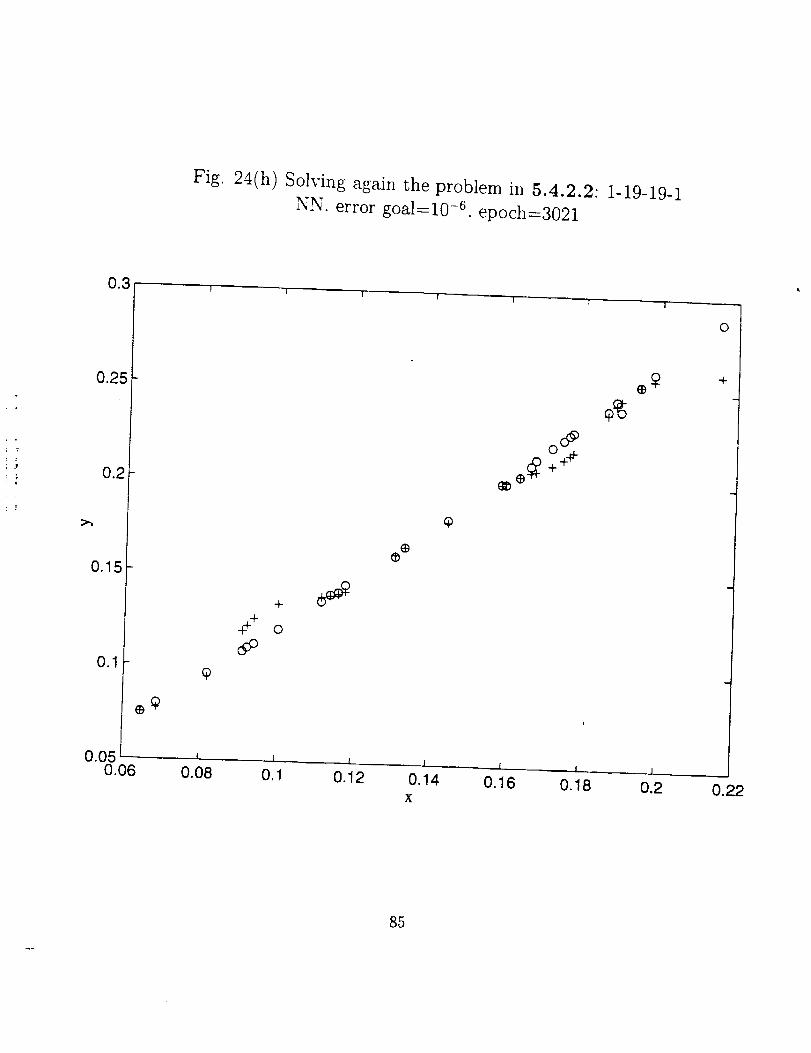
Fig. 24(h) Solving again the problem in 5.4.2.2:1-19-19-1

NN. error goal=10-6, epoch=3021

O

0.25

0.15

+

0

+

0.050.06

0.22

85

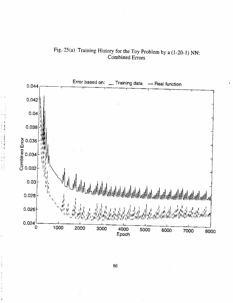
Fig. 25(a) Training History for the Toy Problem by a (1-20-I) NN:Combined Errors

0.044Error based on: __ Training data -- Real function

0.042

0.04

0.038

_,°°3°_1o.o34t-",I',&

0.032_-I';,, 'k I

t'i!0.03 , ,_1

0.028 - " I

O.026

0.0240

tI I _ ! l l I

1000 2000 3000 4000 5000 6000 7000 8000

Epoch

86

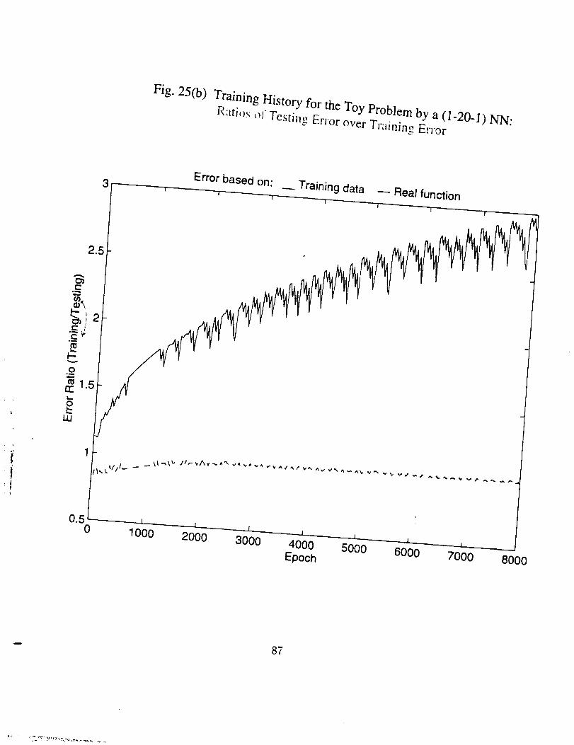
Fig. 25(b) Training History for the Toy Problem by a (1-20-1) NN:

R'ati_s ,_1 Testing Error over Training Error

3

Error based on: _Training data -- Real function

I I I I I

1 , I I I I , I .....

2000 3000 4000 5000 6000 7000

Epoch

8OOO

87

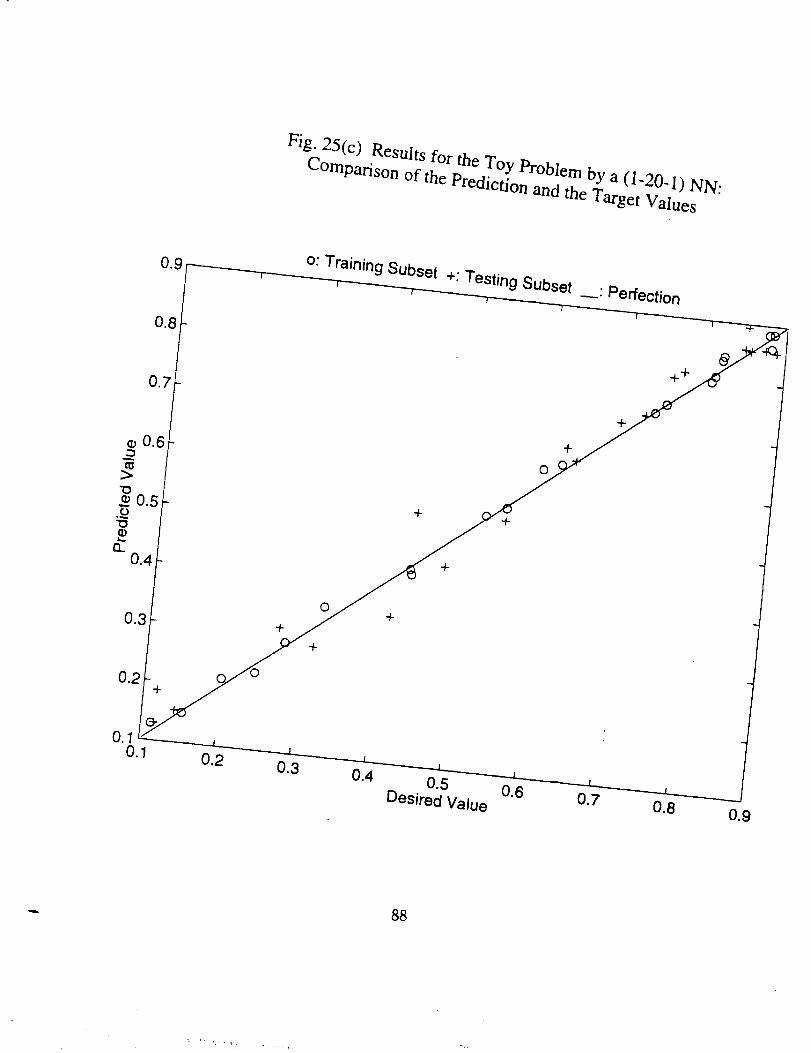
Fig. 25(c) Results for the Toy Problem by a (1-20-1) NN:

Comparison of the Prediction and the Target Values

o: Training Subset +: Testing Subset"Perfection

++

+

+

+

0

+

+

+

+

0

+

+

0.5 0.6Desired Value 0.7

88

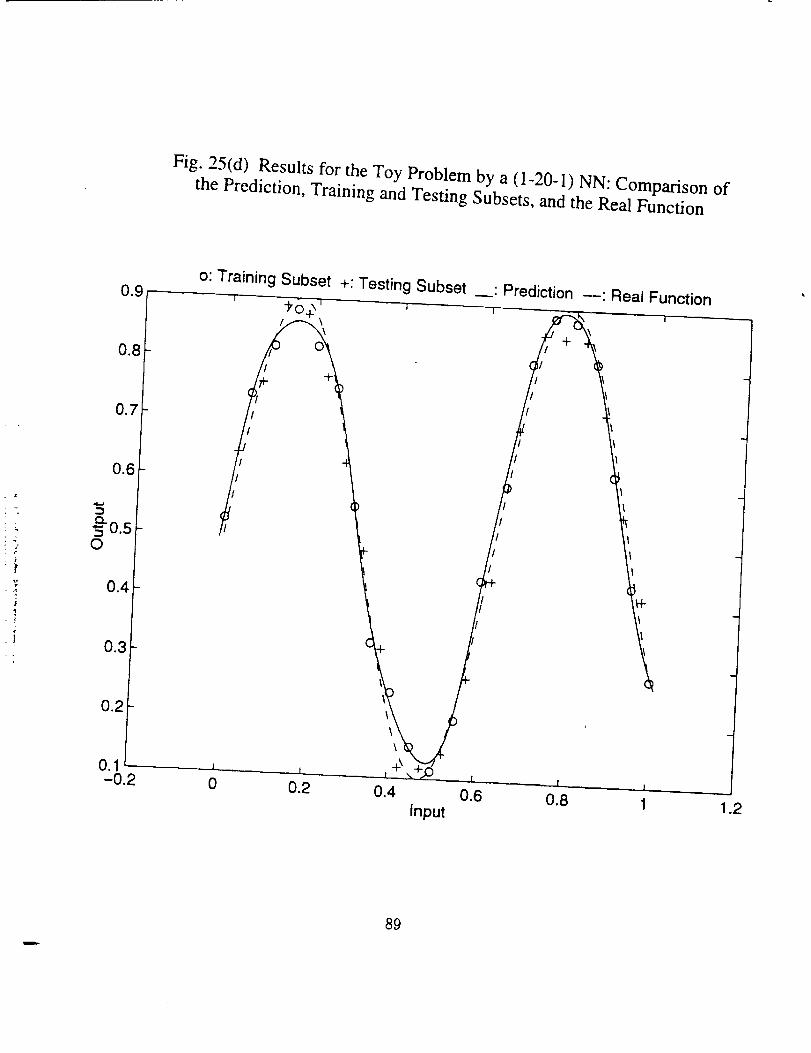
Fig. 25(d) Results for the Toy Problem by a (1-20-1) NN: Comparison of

the Prediction, Training and Testing Subsets, and the Real Function

o: Training Subset +: Testing Subset " Prediction __: Real Function

/ \

" /

i I

t-

I I0 0.2 0.4 0.6 0.8 1

Input 1.2

89

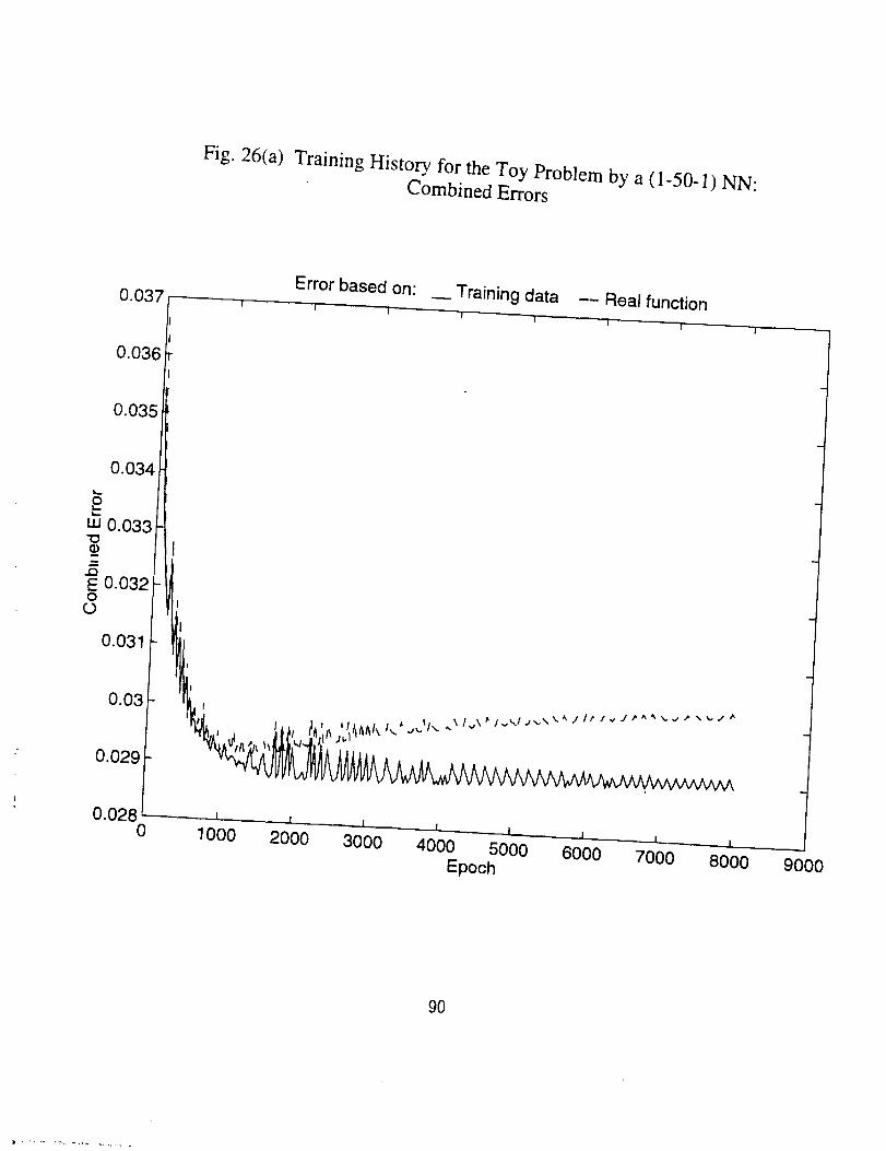
Fig. 26(a) Training History for the Toy Problem by a (1-50-1) NN:Combined Errors

0.037Error based on: _Training data -- Real function

0.036

0.035

0.034

t.u 0.033"O

E 0.032Oo

0.031

0.03

0.029

0.028 1. ..i , , , I I i0 1000 2000 3000 4000 5000 6000 7000 8000

Epoch

9000

90

Fig. 26(b) Training History for the Toy Problem by a (1-50-l) NN:

R_tios or Testify,, Error over Tr:tinin,, Error

Error based on:3O

_ 25

e-

Training data -- Real function

_------------T-----------r----_---r

5

0I I I I I 1

1000 2000 3000 4000 5000 6000 7000 8000Epoch

0

9000

91

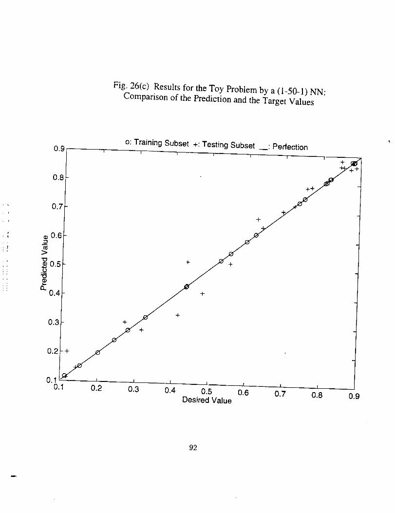
Fig. 26(c) Results for the Toy Problem by a (1-50-1) NN:

Comparison of the Prediction and the Target Values

!

o: Training Subset +: Testing Subset __. Perfection

I I I I l

++

+

+ +

+

I

+

+

+

+

0.2 +

I

0.2I I

0.5Desired Value

I

0.7

92

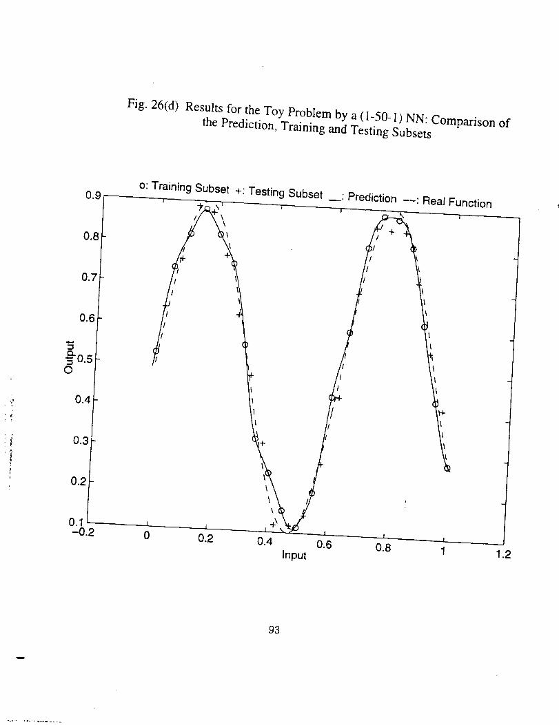
Fig. 26(d) Results for the Toy Problem by a (1-50-1) NN: Comparison ofthe Prediction, Training and Testing Subsets

o: Training Subset +: Testing Subset

\\

• Prediction __: Real Function

0.6

0.50

0 0.2

\

\

0.6 0.8 1Input 1.2

93

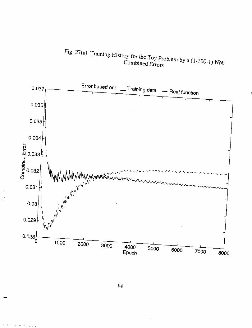
Fig. 27(a) Training History for the Toy Problem by a (I-100-1) NN:

Combined Errors

0.037

Error based on: m Training data -- Real function

| I I 1 I

0.036

0.035

0.034

uJ 0.033'1

.__d_E 0.032OO

0.031

0.03

0.029

0.028 i i ,0 1000 2000 3000

vl

! I

4000 5000

Epoch

I I

6000 7000 8000

94

Fig. 27(b)

Training History for the Toy Problem by a (1-100-1) NN:Ratios of Testing Error over Training Error

100 Error based on: _ Training data -- Real function

9O

8O

2O

10

00 1000

2000 3000 4000 5000Epoch

6000 7OOO 8O0O

95

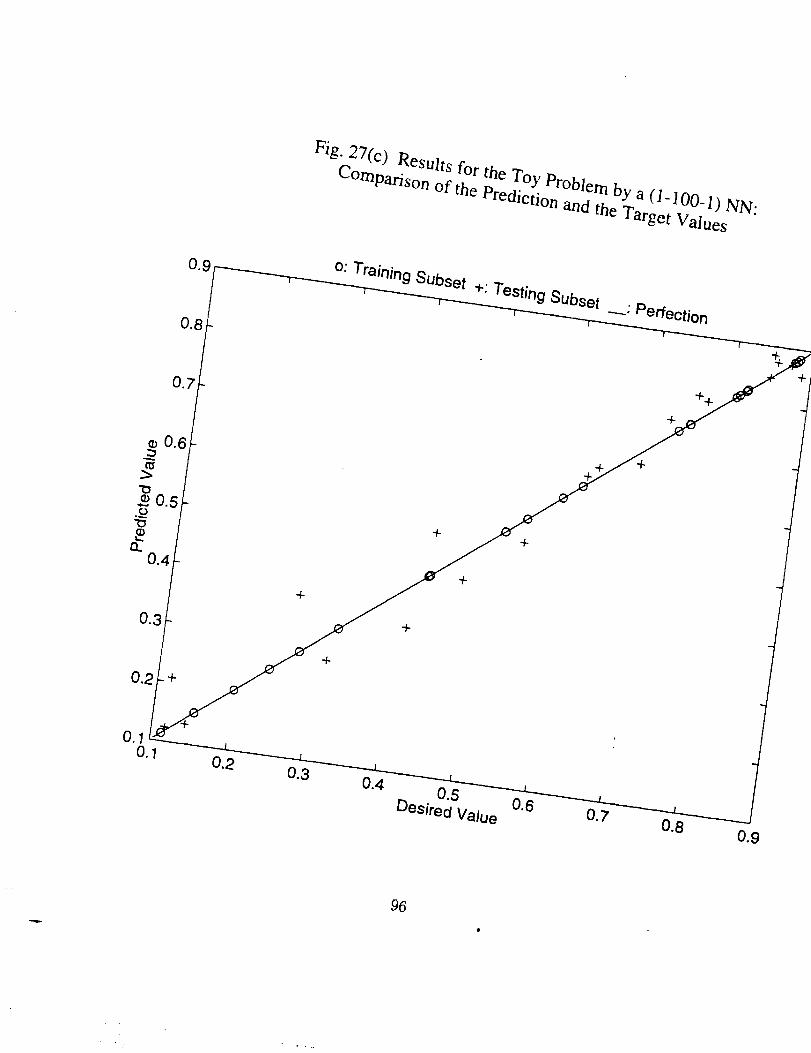
Fig-27(c) Results for the Toy Problem by a (I-100-I) NN:

L'°mparison of the Prediction and the Target Values

o: Training SUbset ÷: Testing Subset

----" Perfection

÷

÷

+

÷

÷

+

+÷

0.50.6

Desired Value 0.7

96

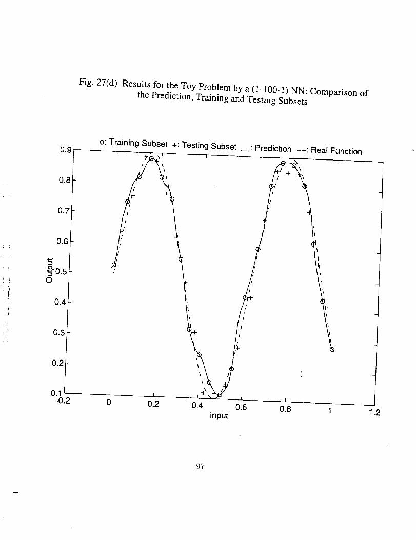
Fig. 27(d) Results for the Toy Problem by a (I-100-I) NN: Comparison ofthe Prediction, Training and Testing Subsets

0.2

0.1 t

-0.2

o: Training Subset +: Testing Subset

1 [

0 0.2

\

\

+\

0.4

Input

' Prediction --: Real Function

II

/

I

I

97

Fig. 28(a) Training History for the Toy Problem by a (1-20-20-1) NN:Combined Errors

0.07

0.06

Error based on:

I

Training data

| I

-- Real function

0.03

\

\

\

I I

0 1000 20001 I

3000 4000

Epoch

1

5000.I

6000I

70O0 8OO0

98

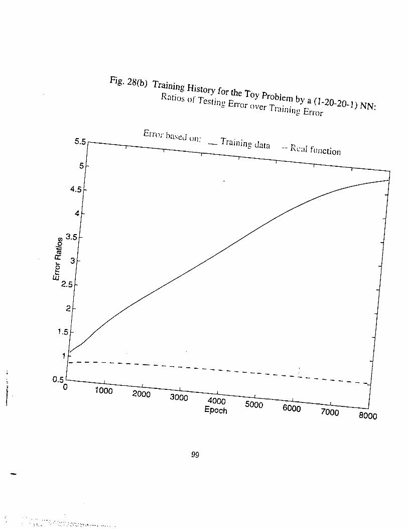
Fig. 28(b)

Training History for the Toy Problem by a (1-20-20-1) NN:Ratios o/ Testing Error (wet Training Error

5

Training data

4

2

0.50

1000 2000 3000

4000 5000 6000Epoch 7000

8000

99

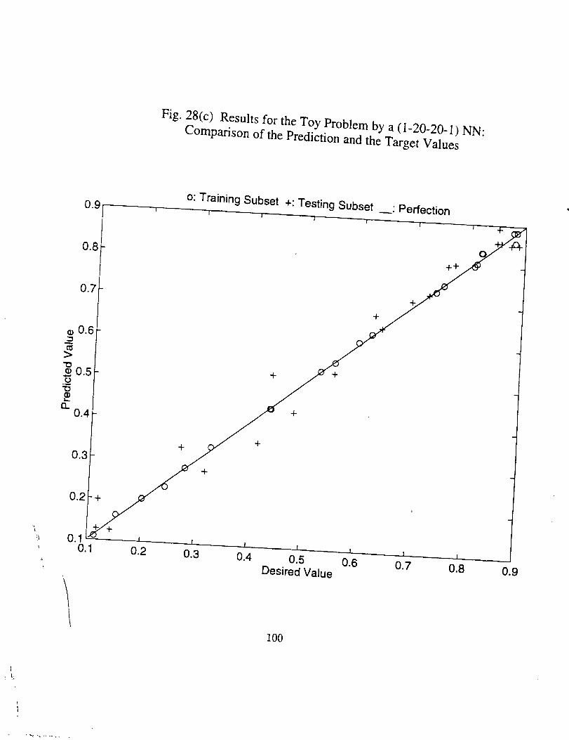
Fig. 28(c) Results for the Toy Problem by a (I-20-20-1) NN:

Comparison of the Prediction and the Target Values

o: Training Subset +: Testing Subset " Perfection

++

+ +

+

+

t

0.2 +

+

+

+

0.5 0.6 0.7Desired Value

100

0.8 0.9

Fig. 28(d)

Results for the Toy Problem by a (1-20-20-1) NN: Comparison ofthe Prediction, Training and Testing. Subsets

o: Training Subset +: Testing Subset"t'0 x

\

Prediction

_'0.50

0

Input

101

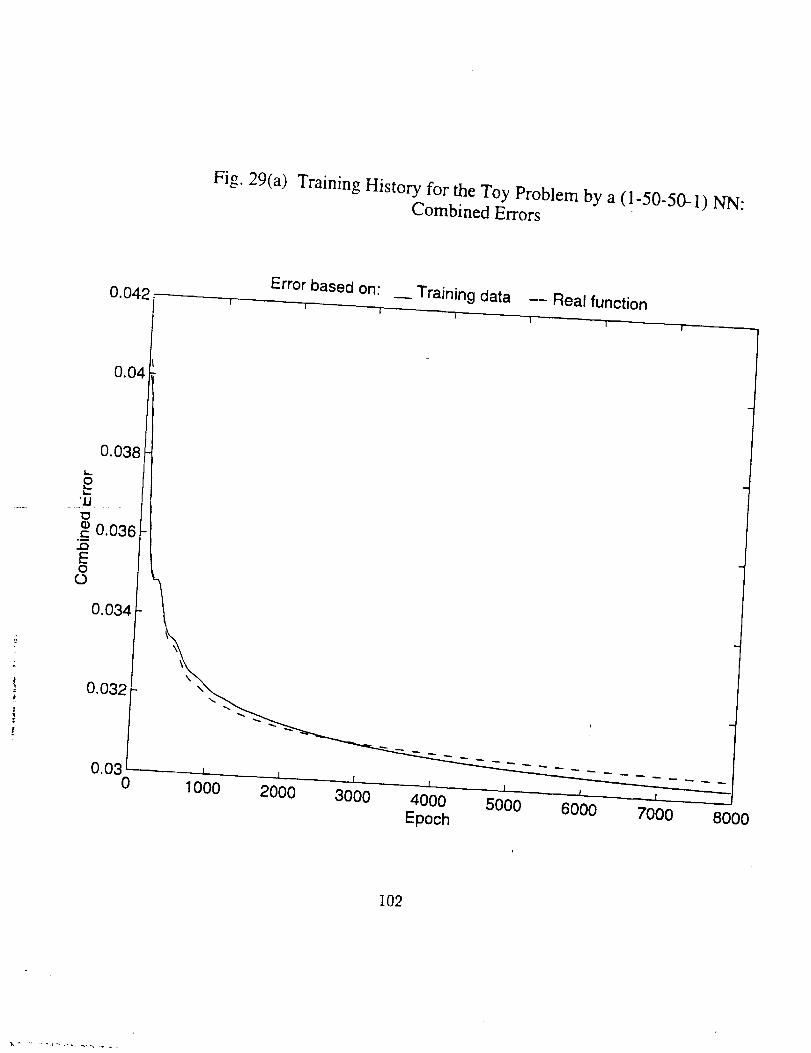
Fig. 29(a) Training History for the Toy Problem by a (1-50-50-1) NN:Combined Errors

0.042Error based on: __ Training data -- Real function

I I | | 1

0.04

0.038

0.034

0.032

0.030

I I 1 l J I

1000 2000 3000 4000 5000 6000 7000Epoch

8000

102

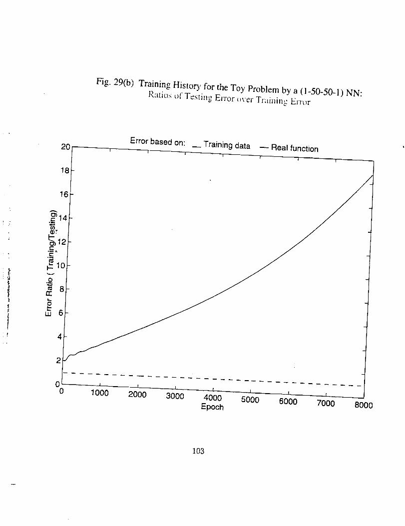
Fig. 29(b)Training History tbr the Toy Problem by a (1-50-50-1) NN:

l'_atios of Testing Error _wer Training Error

2O Error based on: _ Training data -- Real function

18

16

2

00 1000 L__ J l I

2000 3000 4000 5000 6000 7000Epoch

I

800O

103

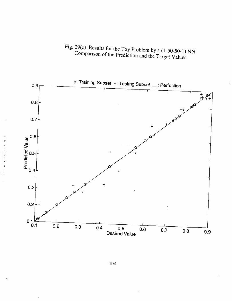
Fig. 29(c) Results for the Toy Problem by a (1-50-50-1) NN:

Comparison of the Prediction and the Target Values

o: Training Subset +: Testing Subset • PerfectionI "t i I

++

+

+ +

+

++

+

I I

0.2 0.3

I ! I I !

0.4 0.5 0.6 0.7 0.8Desired Value

+

104

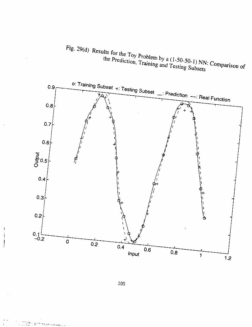
Fig. 29(d)

Results for the Toy Problem by a (1-50-50-I) NN: Comparison ofthe Prediction, Training and Testing Subsets

o: Training Subset +: Testing Subset"Prediction

--: Real Function

/i I

/

0

\

Input1.2

108

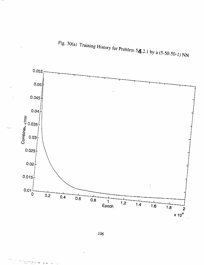
Fig. 30(a)

Training History for Problem 54.2" l by a (5-50-50_ 1) NN

0.055

0.05

0.045

,.. 0.04/

"'J 0.035/-

0.03/-

0.025 -

0.02

0.015/

0.01 L0

Epoch 1.4 1.6 1.8 2

x 104

I06

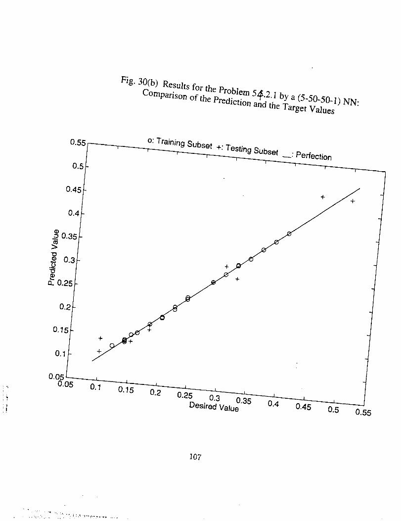
Fig. 30(b) Results for the Problem 54;.2. I by a (5-50-50_ I) NN:

Comparison of the Prediction and the Target Values

0.55_°: Training Subset +: Testing : PerfectionSubset

o:/0.4

/_ o.35

ca.0.25

0.15

0.050.05

0.15

0.25 0.3 0.35 0.4 0.45Desired Value 0.5

0.55

107

., i _?'i_'•_ • _:_ ,-_- ........

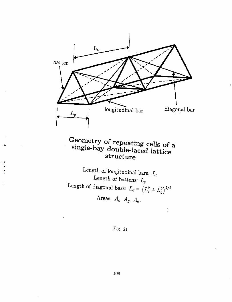
batten

longitudinal bardiagonal bar

Geometry of repeating cells of asingle-bay double-laced lattice

structure

Length of longitudinal bars: Lc

Length of battens: Lg

Length of diagonal bars: Ld = (L_ + L_)1/2

Areas: Ac, Ag, Ad.

Fig. 3]

108

#.

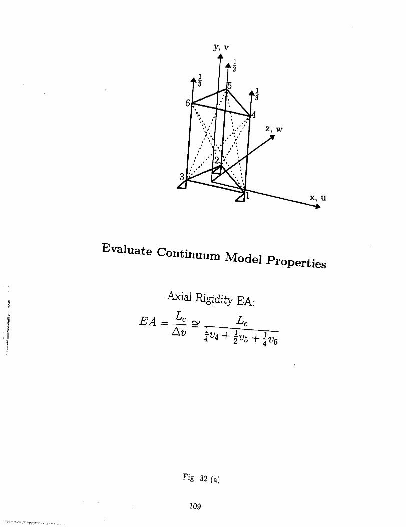
y_ v

+J ,

1

.i ,+

ii

i i ++I+I+ + i • i

", " + ,'. Z+ Wq +I I Io •

+ ++

l.l+ • I,+ I+ i + II

l <+. +i. ++I+ 1 il ,i

• . ++ • ++

i •

++ r

X_ U

Evaluate Continuum Model Properties

1

Axial Rigidity EA:

Lc LcEA=--

Av :'v_+ _.v,:,+ ¼_+,

Fig. 32 (a)

109

_ p. + ,_.....+ .st%+_v +,+.-t + ......

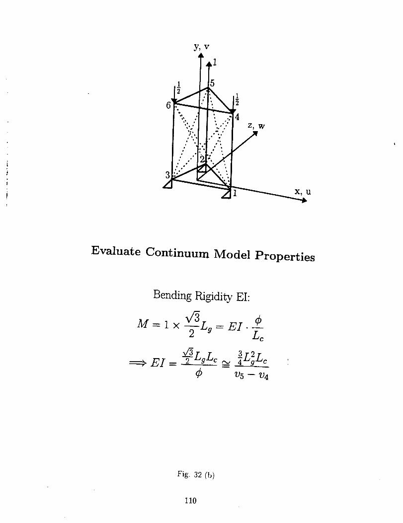
1 5

6'

• .. '.'. Z, W• a "o •

3 ,:i-"' ""

Evaluate Continuum Model Properties

Bending Rigidity El:

v3- ¢M = 1 x --_g : EI.L---_c

E1 = -_LqL_¢

3 2_LgLc

V 5 -- V 4

Fig. 32 (b)

110

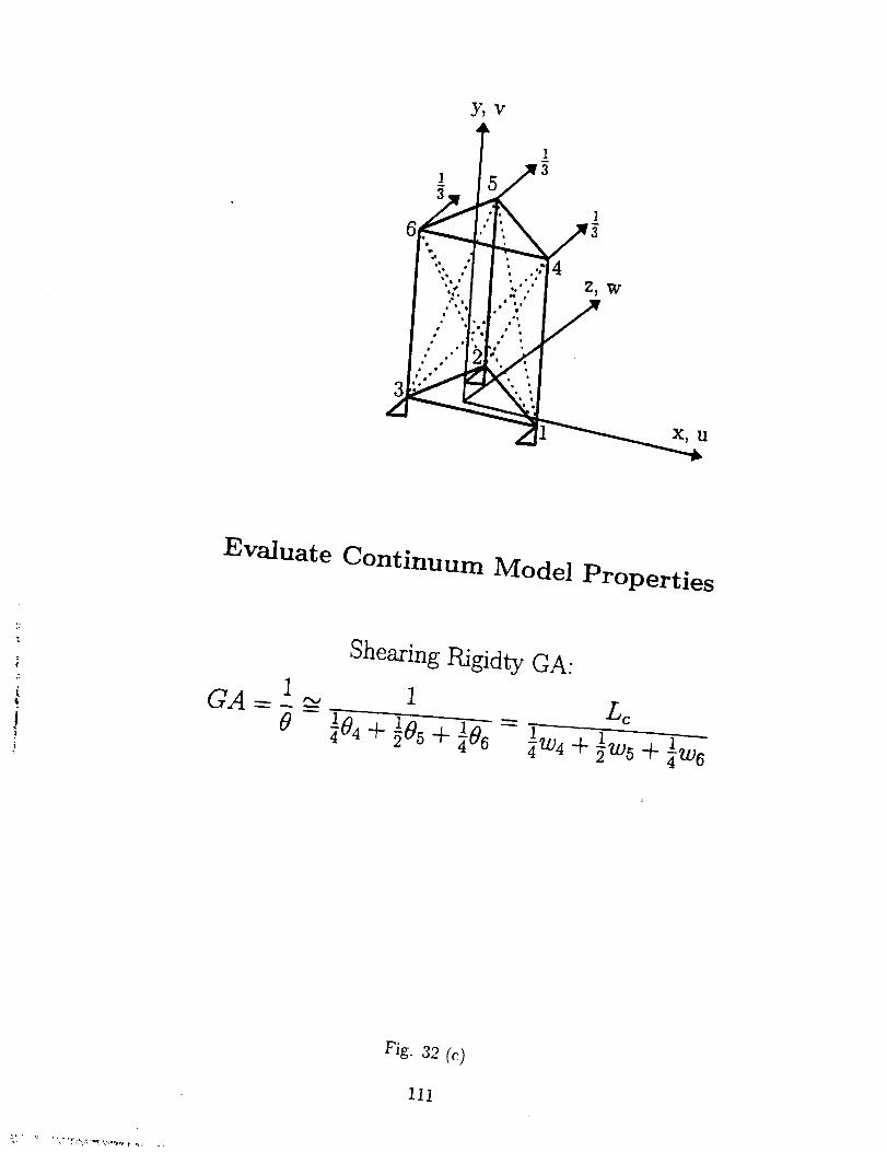
y,v

6 -

""' "/I z,w.e _f

X_ tl

Evaluate Continuum Model Properties

1

8

Shearing Rigidty GA.

1

2 5 _- _6 _w4 + 5w5 + _w6

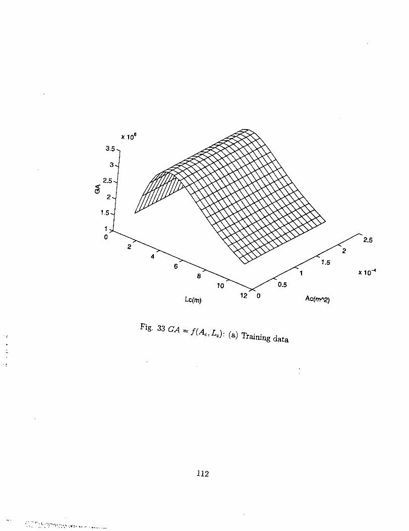
x 10s

2

6

8

Lc(m)

1.5

1

10 0.5

12 0 Ac(,rnA2)

x 10_

Fig.

33 CA = f(Ac, Lc): (a) Training data

112

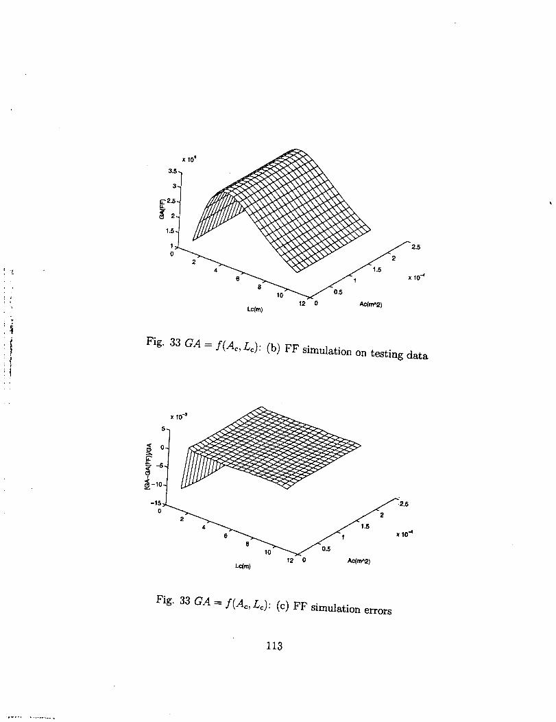
xl

3.5-

3-

_._._2.5.

1.5.

,,k_ _',._

4 6__.,_ _ • -4

1.5 x 101.5 _1_6

- ,o---..._ o._12 0 Ac(rr_2)

Lc(m)

Fig. 33 CA = f(Ac, Lc): (b) FF simulation on testing data

5 xl0_

0 2 2

6" _,,._ Jl x 10"4

8 10 0.5

12 0 Ac(mA2)Lc(m)

Fig. 33 CA = f(Ac, Lc): (c) FF simulation errors

113

xl

3.5.

3.

E

1.5 _

;J ,.,

10 0.5

12 0 Ac.,,A,,,Lc(m)

Fig. 33 CA = f(Ac, Lc): (d) RBF simulation on testing data

0.1

_-_ 0,05.

_ o.--0.05

0

4 _ / ,.5

10 0.5

Lc(m) 12 0 Ac(m_2)

Fig. 33 CA = f(Ac, Lc): (e) RBF simulation errors

114

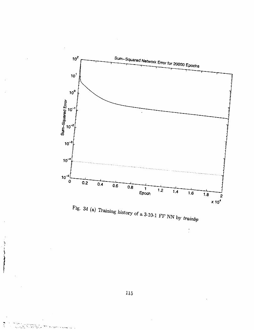
10 2 .,,Sum-Squared Network Errorfor 20000 Epochs

i .... i .... [ i "1 1 ' _ --1 I ' "

101

100

LU

•_ 10-I

10-_O3

10-a

10 "4

10-s0

I , |, .. I , l , I I l ., I . ]

0.2 0.4 0.6 0.8 1 1.2 1.4 1.6 1.8 2

Epoch x 10 4

Fig. 34 (a) Training history of a 3-10-1 FF NN by trainbp

i

115

• _ , _,, -_: ,,._ _-,.,

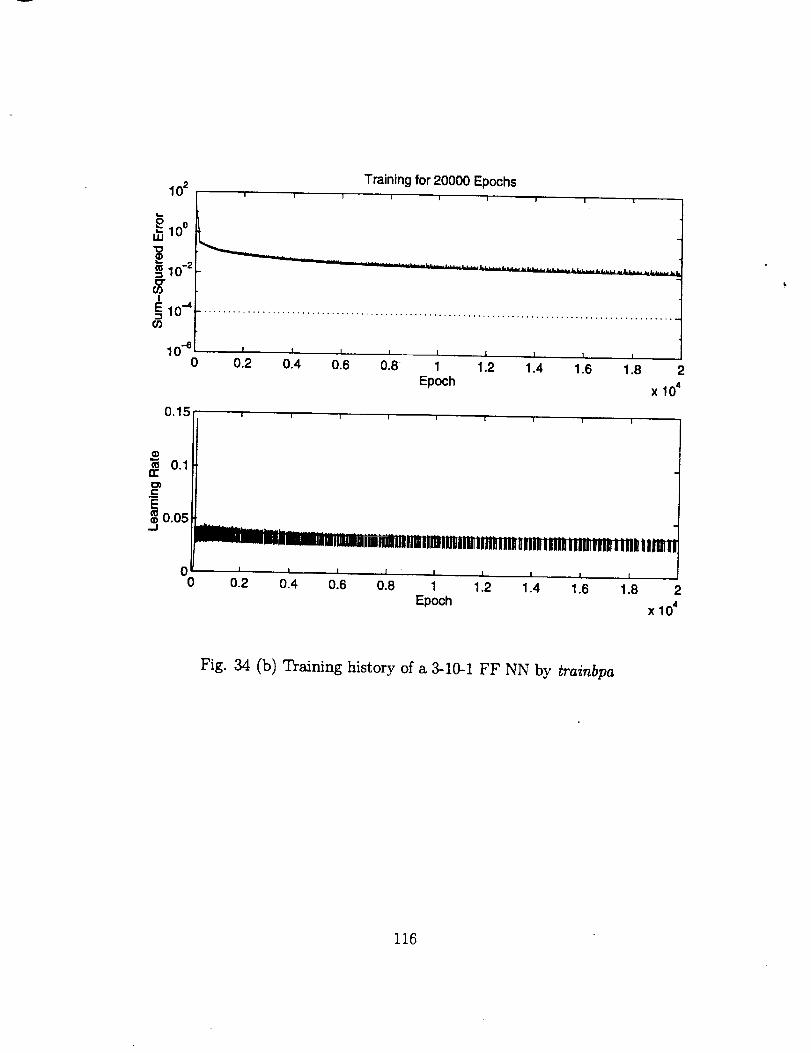
Training for 20000 Epochs

•- 102_| ' ' ' ' ' ' ' ' ' 1

/0 0.2 0.4 0.6 0.8 1 1.2 1.4 1.6 1.8 2

Epoch x 104

0.15 ! I I 1 ] [ 1 I !

"_ 0.1rr

cE

3 0.05

00

I | I ,l I I ,, ! ,J, I

0.2 0.4 0.6 0.8 1 1.2 1.4 1.6 1.8Epoch

2

x 104

Fig. 34 (b) Training history of a 3-10-1 FF NN by trainbpa

116

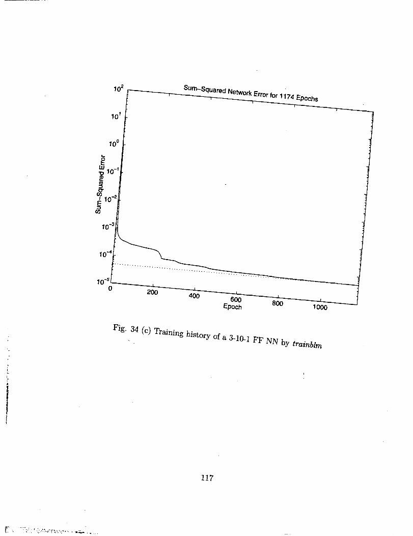
Sum-Squared Network Error for 1174 Epochs

100

200400 600

Epoch 800 1000

Fig.. 34 (c) Training history of a 3-10-1 FF NN by trainblrn

117