artificial bee colony using mpi - university at buffalo · artificial bee colony algorithm using...
TRANSCRIPT

Artificial Bee Colony Algorithm
using MPI
Pradeep Yenneti
CSE633, Fall 2012
Instructor : Dr. Russ Miller
University at Buffalo, the State University of New York
OVERVIEW
Introduction
Components
Working
Artificial Bee Colony algorithm (RAM)
Artificial Bee Colony algorithm (Parallel)
Performance
An Alternative Parallel Approach
Observations / Limitations
Future goals
References

INTRODUCTION
Artificial Bee Colony (ABC) algorithm is a swarm-based meta-heuristic optimization algorithm.
Algorithm based on the foraging behavior of bees in a colony.
Applications :
Optimal multi-level thresholding, MR brain image classification, face pose estimation, 2D protein folding

COMPONENTS
Food Source :
A food source location denotes the possible solution (vector with n parameters) .eg. Amount of food in the source denotes quality (fitness).
Employed Bees :
Retrieve food from source and report back neighboring sources. One bee per source.
Scout Bees :
Find and update different sources. Employed bees whose food source is exhausted become Scout bees.
Onlooker Bees :
Choose food source based on inputs from Employed bees.
WORKING
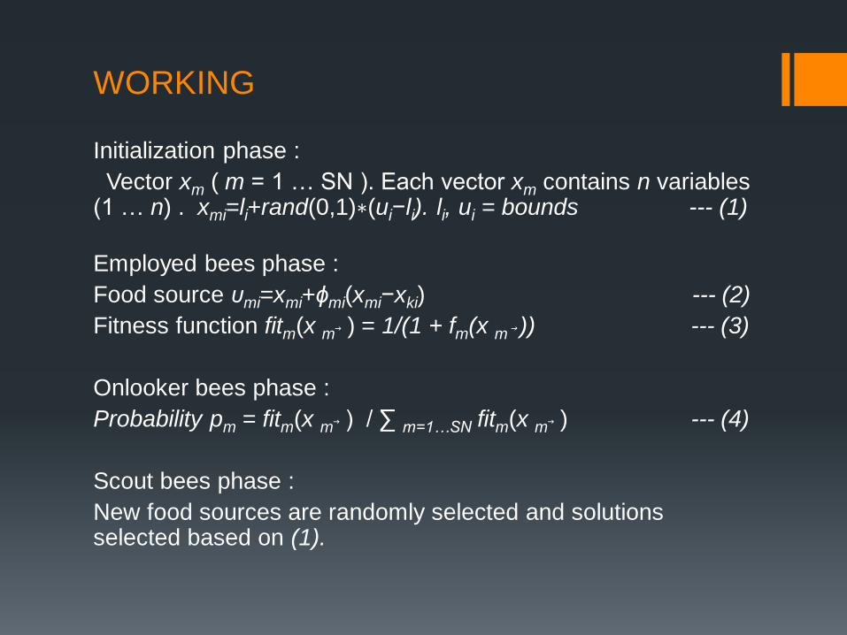
Initialization phase :
Vector xm ( m = 1 … SN ). Each vector xm contains n variables (1 … n) . xmi=li+rand(0,1)∗(ui−li). li, ui = bounds --- (1)
Employed bees phase :
Food source υmi=xmi+ϕmi(xmi−xki) --- (2)
Fitness function fitm(x m⃗ ) = 1/(1 + fm(x m⃗ )) --- (3)
Onlooker bees phase :
Probability pm = fitm(x m⃗ ) / ∑ m=1…SN fitm(x m⃗ ) --- (4)
Scout bees phase :
New food sources are randomly selected and solutions selected based on (1).

WORKING

WORKING
1 4.113152 7.630029 18.6177 9.005129 17.91446
2 9.935555 13.37011 4.745863 10.6545 19.78366
3 10.95558 19.49226 17.84674 10.75404 18.06841
4 18.53284 0.792465 18.59932 3.516931 14.82533
5 14.34575 3.136435 5.886008 6.576565 7.916828
6 17.86021 14.02121 17.46455 14.59524 16.75909
7 3.731504 5.224778 16.29288 11.44785 0.314989
8 0.627248 13.82126 3.269592 13.46171 13.24224
Serial representation – n Rows, single processor (n food sources)

WORKING
1 4.113152 7.630029 18.6177 9.005129 17.91446
2 9.935555 13.37011 4.745863 10.6545 19.78366
3 10.95558 19.49226 17.84674 10.75404 18.06841
4 18.53284 0.792465 18.59932 3.516931 14.82533
5 14.34575 3.136435 5.886008 6.576565 7.916828
6 17.86021 14.02121 17.46455 14.59524 16.75909
7 3.731504 5.224778 16.29288 11.44785 0.314989
8 0.627248 13.82126 3.269592 13.46171 13.24224
Parallel representation - n Rows split among m processors
(n/m food sources per processor)

DATA AND PROCESSORS USED
Programming Language : C++ with MPI
# of Processors : 1-16. 8 cores per processor. (Total 128 cores).
Size of data (data type = float):
• 65536 X 5
• 65536 X 40
• 512000 X 10
• 768000 X 10
• 8192 X 20
Upper limit = 10, Lower limit = -10
Criterion for termination of program :
• global_minimum = 0.000001 (OR) max_cycle = 1000
Number of runs for each data set and processor # : 10
Functions used :
• Sphere : f(x) = Ʃ xi2 (i = 1 – D)
• Rastringin : f(x) = Ʃ (xi2 - 10*cos(2π*xi)
+10 ) --- (i = 1 – D)

RAM ALGORITHM
Start
Initialize parameters
Initial solution
REPEAT
o Find and evaluate solution by Employed bees
o Select and update food source by Onlooker bees
o Evaluate solution by Onlooker bees
o If solution is abandoned, generate new solution by
Scout bees
UNTIL criteria are met
End

PARALLEL ALGORITHM
Start
Initialize parameters
Divide populations into sub-groups for each processor
Initial solution
REPEAT
o Find and evaluate solution by Employed bees
o Select and update food source by Onlooker bees
o Evaluate solution by Onlooker bees
o If solution is abandoned, generate new solution for Scout bees
o Exchange information within sub-groups (local worst/best solutions)
UNTIL criteria are met
End

PARALLEL ALGORITHM
1. For each cycle, Processor 0 generates random pairs
and communicates the pairing to the remaining
processors (MPI_Send, MPI_Recv)
2. At the end of each cycle, the processors replace the
local worst solution with the local best solution
obtained from their respective partners.
3. After the desired criteria are met, the processors
exchange local best solutions and receive the overall
best solution (MPI_Allreduce)

VALUES OBTAINED
Time taken for different data sizes and # cores
Input data = #Food sources, #Parameters per food
source
65536, 40 65536, 5 512000, 10 8192, 20 768000, 10
1 970.23 38.11 448.37 37.56 677.45
2 513.21 19.21 227.46 19.13 344.87
4 269.41 9.94 114.34 9.61 174.15
8 139.84 5.42 59.26 4.98 88.85
16 71.91 2.96 30.32 2.69 45.77
32 37.81 1.59 15.96 1.32 23.06
64 19.83 0.92 8.33 0.83 12.40
128 10.67 0.51 4.62 0.65 6.57

PERFORMANCE – Time vs # cores
0.10
1.00
10.00
100.00
1000.00
0 20 40 60 80 100 120 140
T
i
m
e
(
s
e
c
o
n
d
s)
# Cores
65536, 40
65536, 5
512000, 10
8192, 20
768000, 10

PERFORMANCE - speedup
0.000
20.000
40.000
60.000
80.000
100.000
120.000
140.000
0 20 40 60 80 100 120 140
S
p
e
e
d
u
p
# cores
65536, 40
65536, 5
512000, 10
8192, 20
768000, 10
Ideal

AN ALTERNATIVE PARALLEL APPROACH
Best solutions are not exchanged between processors
between cycles.
After criteria are met, Local best solutions are
exchanged between processors and the overall best
solution is chosen.

VALUES OBTAINED
Time taken for different data sizes and # cores
Input data = #Food sources, #Parameters per food
source
65536, 40 65536, 5 512000, 10 8192, 20 768000, 10
1.00 970.23 38.11 448.37 37.56 677.45
2.00 506.11 19.83 230.47 19.04 344.03
4.00 263.85 10.51 116.64 9.89 175.59
8.00 138.73 5.89 61.72 5.06 89.67
16.00 69.34 3.05 20.15 2.67 45.65
32.00 35.29 1.61 15.22 1.45 22.89
64.00 18.64 0.89 8.14 0.92 12.08
128.00 9.45 0.48 4.45 0.63 6.26

PERFORMANCE – Comparison of both
approaches
1.00
10.00
100.00
1000.00
1.00 10.00 100.00 1000.00
T
i
m
e
(
s
e
c
o
n
d
s)
# Cores
65536, 40 - II
65536, 40 - I
768000, 10 - II
768000, 10 - I

OBSERVATIONS / LIMITATIONS
Time taken to execute increases based on the number
of Food Sources (linear) and number of Parameters
per Food Source (non-linear, possibly polynomial).
For a given number of processors, speedup increases
as the number of parameters. (Increase w.r.t. time in
inter-process communication is linear while increase
within each processor is non-linear).
For a fixed number of food sources, speedup gradually
decreases as the number of processors increase, as
seen in the speedup of the data set (8192 X 20).

OBSERVATIONS / LIMITATIONS
For a lower number of processors, the first parallel
approach was found to be (marginally) faster.
As the number of processors increases, the alternative
approach appears to be (marginally) faster. Less
communication is a factor.
Beyond a certain number of parameters (eg.20), the
output does not converge adequately even after >
1000 cycles

FUTURE GOALS
Implement in OpenMP and CUDA
Compare performances between MPI, OpenMP and
CUDA
REFERENCES
Artificial bee colony algorithm on distributed environments (Banharnsakun, A.; Achalakul, T.; Sirinaovakul, B.) http://ieeexplore.ieee.org/xpl/login.jsp?tp=&arnumber=5716309&url=http%3A%2F%2Fieeexplore.ieee.org%2Fxpls%2Fabs_all.jsp%3Farnumber%3D5716309
A powerful and efficient algorithm for numerical function optimization : artificial bee colony (ABC) algorithm (D. Karaboga, B. Basturk) http://www.springerlink.com/content/1x7x45uw7q7w3x35/
A comparative study of Artificial Bee Colony algorithm
http://chern.ie.nthu.edu.tw/gen/comparative-study.pdf
http://en.wikipedia.org/wiki/Artificial_bee_colony_algorithm

QUESTIONS ?

THANK YOU