artificial intelligence - vilniaus universitetascyras/ai/ai-cyras.pdf · artificial intelligence,...
TRANSCRIPT
Vilnius University
Faculty of Mathematics and Informatics
Institute of Computer Science
Vytautas Čyras
ARTIFICIAL INTELLIGENCE
https://www.mif.vu.lt/~cyras/AI/ai-cyras.pdf
Vilnius
2020
- 2 -
Artificial Intelligence, 18-05-2020
Table of Contents
1. Introduction ........................................................................................................................ 5
1.1. The subject matter of artificial intelligence ................................................................ 5
1.2. The Towers of Hanoi .................................................................................................. 7
1.3. Dynamic nature of artificial intelligence ................................................................... 10
1.4. Methods of problem solving ..................................................................................... 11
2. Artificial intelligence system as a production system .................................................... 12
2.1. Testing ....................................................................................................................... 16
3. Control with backtracking and procedure BACKTRACK .......................................... 17
3.1. An example of the DEADEND predicate ................................................................. 18
4. The 8-queens puzzle.......................................................................................................... 19
5. Heuristic ............................................................................................................................ 22
5.1. Heuristic search in N-queens problem ...................................................................... 22
5.2. Knight’s move heuristic in the N-queens problem ................................................... 25
6. BACKTRACK1 – a cycle-avoiding algorithm ............................................................... 31
7. Depth-first search in a labyrinth ..................................................................................... 32
7.1. Testing depth-first search in a labyrinth .................................................................... 35
8. Breadth-first search in a labyrinth ................................................................................. 37
8.1. Testing breadth-first search in a labyrinth ................................................................ 41
9. Breadth-first search in a graph ....................................................................................... 43
10. Shortest path problem in a graph with edge weights .................................................... 46
11. Depth-first search in a graph with no weights. The solver and the planner ............... 49
12. The prefix, infix and postfix order of tree traversal ...................................................... 51
13. GRAPHSEARCH algorithm ........................................................................................... 56
14. Differences between BACKTRACK1 and GRAPHSEARCH-DEPTH-FIRST ......... 57
14.1. Searching in a graph .................................................................................................. 57
14.2. Multiple cycles in a labyrinth .................................................................................... 58
14.3. A counterexample of better performance with BACKTRACK1 .............................. 60
15. Hill-climbing strategy ....................................................................................................... 62
16. Manhattan distance .......................................................................................................... 65
17. A* search algorithm ......................................................................................................... 67
17.1. Manhattan distance in the tile world ......................................................................... 67
17.2. An example from Russell & Norvig 2003 ................................................................ 70
18. Forward chaining and backward chaining .................................................................... 73
- 3 -
Artificial Intelligence, 18-05-2020
18.1. Forward chaining ...................................................................................................... 73
18.2. Backward chaining .................................................................................................... 74
18.3. Program synthesis ..................................................................................................... 75
18.4. Superfluous rules in forward chaining ...................................................................... 76
18.5. Superfluous rules in backward chaining ................................................................... 77
18.6. Complexity of forward chaining ............................................................................... 77
18.7. Testing forward chaining .......................................................................................... 78
18.8. Testing backward chaining ....................................................................................... 80
19. Resolution .......................................................................................................................... 83
19.1. Inference example ..................................................................................................... 85
19.2. Example with three rules ........................................................................................... 87
19.3. Using resolution to prove theorem ............................................................................ 90
20. Expert systems .................................................................................................................. 91
21. Internet shopping .............................................................................................................. 94
22. The Turing test................................................................................................................ 100
23. Intension, extension and ontology ................................................................................. 101
23.1. Signs ........................................................................................................................ 102
23.2. What is a conceptualization? ................................................................................... 103
23.3. What is a proper formal, explicit specification? ..................................................... 107
23.4. Distinct models of a specification ........................................................................... 112
24. Examination questions ................................................................................................... 115
25. References ........................................................................................................................ 116
- 4 -
Artificial Intelligence, 18-05-2020
Preface
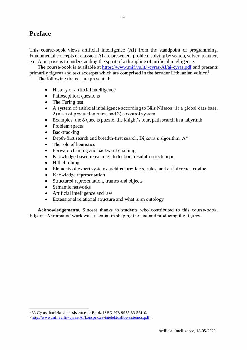
This course-book views artificial intelligence (AI) from the standpoint of programming.
Fundamental concepts of classical AI are presented: problem solving by search, solver, planner,
etc. A purpose is to understanding the spirit of a discipline of artificial intelligence.
The course-book is available at https://www.mif.vu.lt/~cyras/AI/ai-cyras.pdf and presents
primarily figures and text excerpts which are comprised in the broader Lithuanian edition1.
The following themes are presented:
History of artificial intelligence
Philosophical questions
The Turing test
A system of artificial intelligence according to Nils Nilsson: 1) a global data base,
2) a set of production rules, and 3) a control system
Examples: the 8 queens puzzle, the knight’s tour, path search in a labyrinth
Problem spaces
Backtracking
Depth-first search and breadth-first search, Dijkstra’s algorithm, A*
The role of heuristics
Forward chaining and backward chaining
Knowledge-based reasoning, deduction, resolution technique
Hill climbing
Elements of expert systems architecture: facts, rules, and an inference engine
Knowledge representation
Structured representation, frames and objects
Semantic networks
Artificial intelligence and law
Extensional relational structure and what is an ontology
Acknowledgements. Sincere thanks to students who contributed to this course-book.
Edgaras Abromaitis’ work was essential in shaping the text and producing the figures.
1 V. Čyras. Intelektualios sistemos. e-Book. ISBN 978-9955-33-561-0.
<http://www.mif.vu.lt/~cyras/AI/konspektas-intelektualios-sistemos.pdf>.
- 5 -
Artificial Intelligence, 18-05-2020
1. Introduction
American scientist Marvin Minsky defined AI as “the science of making machines do things
that would require intelligence if done by men.”2 A similar definition is “the science of
designing computer systems to perform tasks that would normally require human intelligence”
(Sowa 2000, p. XI). The term “artificial intelligence” was coined in a research project proposed
for the 1956 summer workshop at Dartmouth College in Hanover, New Hampshire, United
States.3 The term is attributed to John McCarthy.4
The term “artificial intelligence” is used to describe machines that mimic “cognitive”
functions that humans associate with other human minds, such as “learning” and “problem
solving”, see (Russell, Norvig 2010, p. 2).
1.1. The subject matter of artificial intelligence
The subject matter of AI also shows the place of AI within the discipline of computer science.
Following is a classification of computing according to the ACM Computing Classification
System in US; see https://www.acm.org/publications/class-2012 by the Association for
Computer Machinery.
General Literature
Hardware
Computer systems organization
Networks
Software
Data
Theory of computation
Mathematics of computing
Information systems
Security and privacy
Human-centered computing
Computing methodologies
Computer applications
Social and professional topics
Artificial intelligence is comprised by the branch Computing methodologies above which
is classified further:
Symbolic and algebraic manipulation
2 See generally Marvin L. Minsky (1968) Introduction, in: Semantic Information Processing, M. L. Minsky (ed.),
MIT Press, Cambridge (Massachusetts). See also https://www.britannica.com/biography/Marvin-Lee-Minsky. 3 John MaCarthy, Marvin Minsky, Nathaniel Rochester, Claude Shannon, A Proposal for the Dartmouth Summer
Research Project on Artificial Intelligence (31 August 1955), AI Magazine, vol. 27 (2006), no. 4, pp. 12–14,
https://www.aaai.org/ojs/index.php/aimagazine/article/view/1904/1802. 4 John McCarthy’s answer to the question “What is artificial intelligence?” is “It is the science and engineering of
making intelligent machines, especially intelligent computer programs. It is related to the similar task of using
computers to understand human intelligence, but AI does not have to confine itself to methods that are biologically
observable.” McCarthy continues answering what intelligence is: “Intelligence is the computational part of the
ability to achieve goals in the world.” McCarthy is sceptical about parallel machines: “Parallelism itself presents
no advantages, and parallel machines are somewhat awkward to program” (see McCarthy 2007, pp. 2–4,
http://www-formal.stanford.edu/jmc/whatisai.pdf).
- 6 -
Artificial Intelligence, 18-05-2020
Parallel computing methodologies
Artificial intelligence Machine learning
Modeling and simulation
Computer graphics
Distributed computing methodologies
Concurrent computing methodologies
Artificial intelligence is classified further:
Natural language processing
o Information extraction; Machine translation; Discourse, dialogue and
pragmatics; Natural language generation; Speech recognition; Lexical
semantics; Phonology / morphology; Language resources
Knowledge representation and reasoning o Description logics; Semantic networks; Nonmonotonic, default
reasoning and belief revision; Probabilistic reasoning; Vagueness and
fuzzy logic; Causal reasoning and diagnostics; Temporal reasoning;
Cognitive robotics; Ontology engineering; Logic programming and
answer set programming; Spatial and physical reasoning; Reasoning
about belief and knowledge
Planning and scheduling
o Planning for deterministic actions; Planning under uncertainty; Multi-
agent planning; Planning with abstraction and generalization; Robotic
planning
Search methodologies
o Heuristic function construction; Discrete space search; Continuous
space search; Randomized search; Game tree search; Abstraction and
micro-operators; Search with partial observations
Control methods
o Robotic planning; Computational control theory; Motion path planning
Philosophical/theoretical foundations of artificial intelligence
o Cognitive science; Theory of mind
Distributed artificial intelligence
o Multi-agent systems; Intelligent agents; Mobile agents; Cooperation
and coordination
Computer vision
o Computer vision tasks
Biometrics; Scene understanding; Activity recognition and
understanding; Video summarization; Visual content-based
indexing and retrieval; Visual inspection; Vision for robotics;
Scene anomaly detection
o Image and video acquisition
Camera calibration; Epipolar geometry; Computational
photography; Hyperspectral imaging; Motion capture; 3D
imaging; Active vision
o Computer vision representations
Image representations; Shape representations; Appearance and
texture representations; Hierarchical representations
o Computer vision problems
- 7 -
Artificial Intelligence, 18-05-2020
Interest point and salient region detections; Image segmentation;
Video segmentation; Shape inference; Object detection/recog-
nition/identification; Tracking; Reconstruction; Matching
What means “artificially intelligent”? Intelligent entities have the abilities to perceive,
understand, predict, and manipulate. AI is related with logic. Logic (from the Ancient Greek
logikḗ, “the word” or “what is spoken” (but coming to mean “thought” or “reason”), is generally
held to consist of the systematic study of the form of arguments. Also related to logos, “word,
thought, idea, argument, account, reason, or principle” (https://en.wikipedia.org/wiki/Logic).
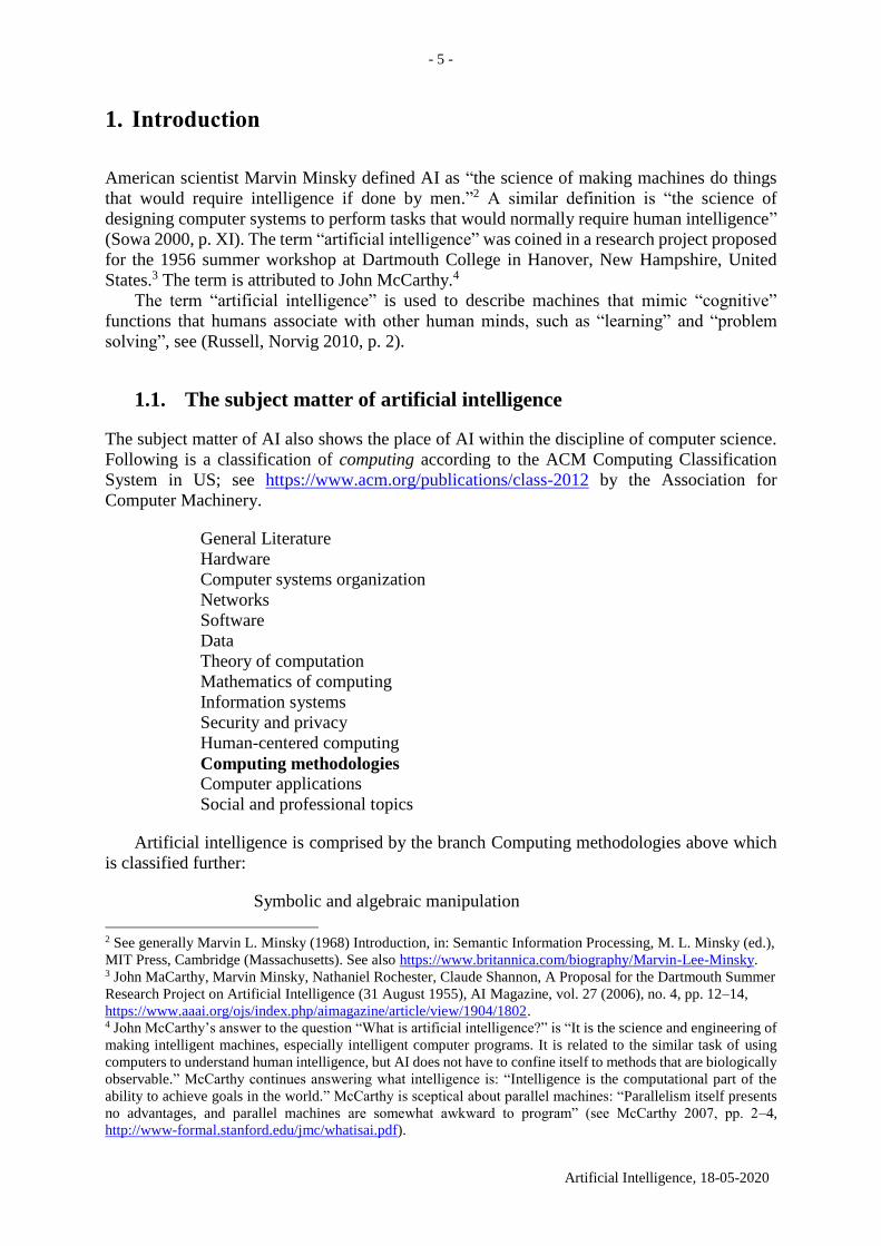
1.2. The Towers of Hanoi
See https://en.wikipedia.org/wiki/Towers_of_Hanoi.
Fig. 1.1. a) Initial state A=(3,2,1), B=(), C=(). b) Terminal state
A=(), B=(), C=(3,2,1)
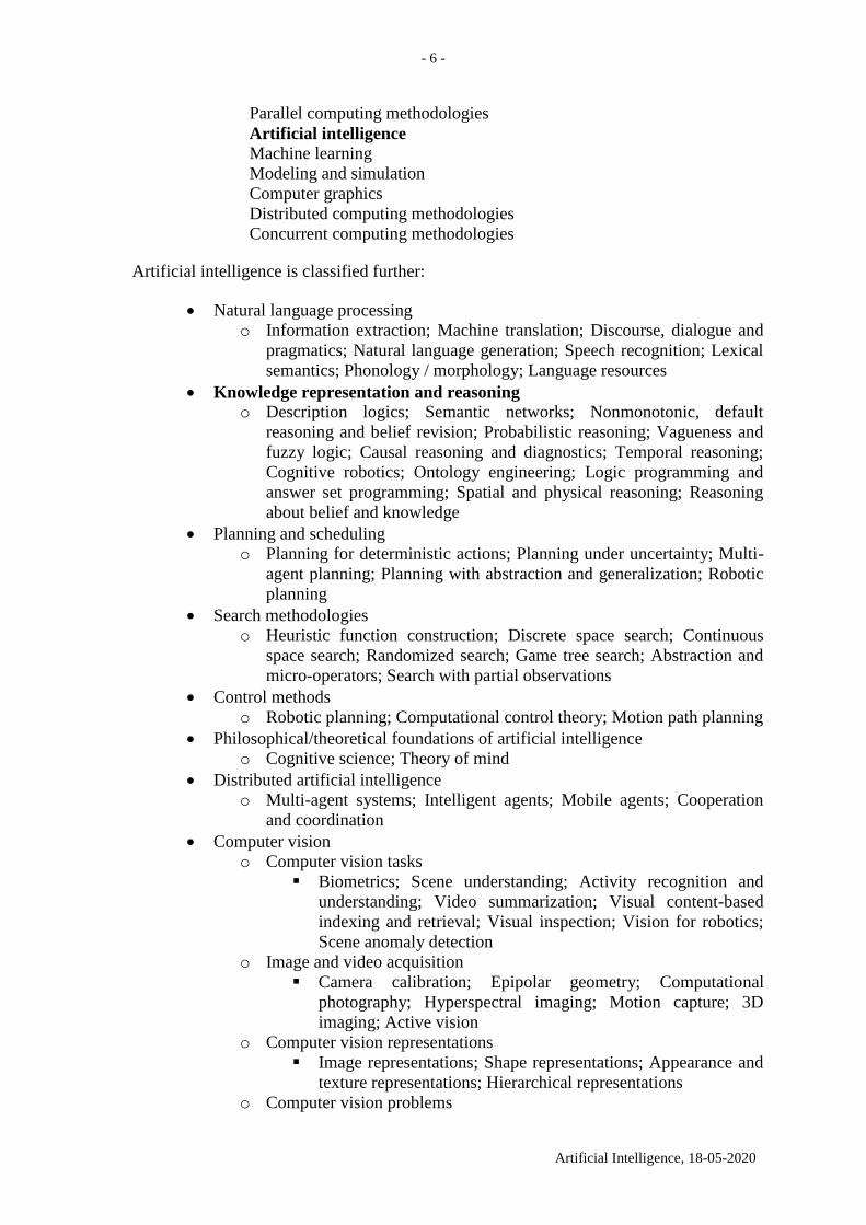
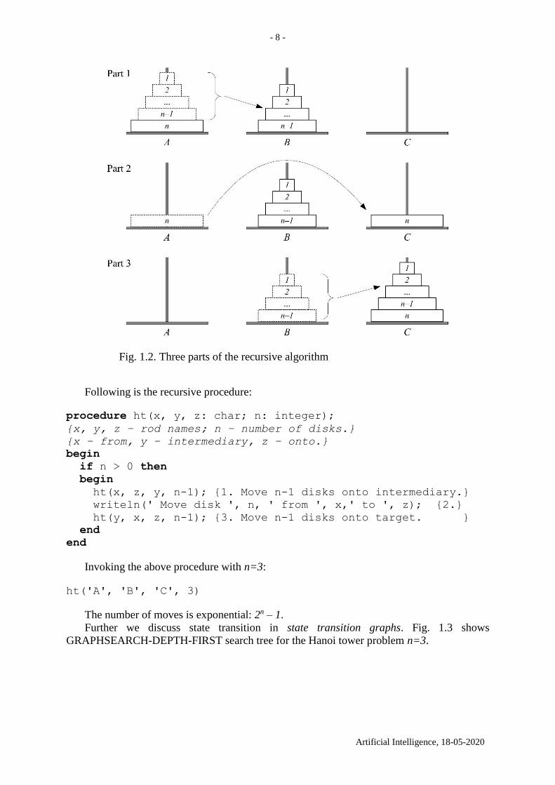
Finding a sequence of moves is an intelligent task. Intelligence is hidden in the recursive
algorithm below (Fig. 1.2):
Part 1. Move n–1 disks from A to B;
Part 2. Move disk n from A to C;
Part 3. Move n–1 disks from B to C.
The sequence of moves for n=3:
Initial state A=(3,2,1), B=(), C=().
1. Move disk 1 from A to C. A=(3,2), B=(), C=(1).
2. Move disk 2 from A to B. A=(3), B=(2), C=(1).
3. Move disk 1 from C to B. A=(3), B=(2,1), C=().
4. Move disk 3 from A to C. A=(), B=(2,1), C=(3).
5. Move disk 1 from B to A. A=(1), B=(2), C=(3).
6. Move disk 2 from B to C. A=(1), B=(), C=(3,2).
7. Move disk 1 from A to C. A=(), B=(), C=(3,2,1).
- 8 -
Artificial Intelligence, 18-05-2020
Fig. 1.2. Three parts of the recursive algorithm
Following is the recursive procedure:
procedure ht(x, y, z: char; n: integer);
{x, y, z – rod names; n – number of disks.}
{x – from, y – intermediary, z – onto.}
begin
if n > 0 then
begin
ht(x, z, y, n-1); {1. Move n-1 disks onto intermediary.}
writeln(' Move disk ', n, ' from ', x,' to ', z); {2.}
ht(y, x, z, n-1); {3. Move n-1 disks onto target. }
end
end
Invoking the above procedure with n=3:
ht('A', 'B', 'C', 3)
The number of moves is exponential: 2n – 1.
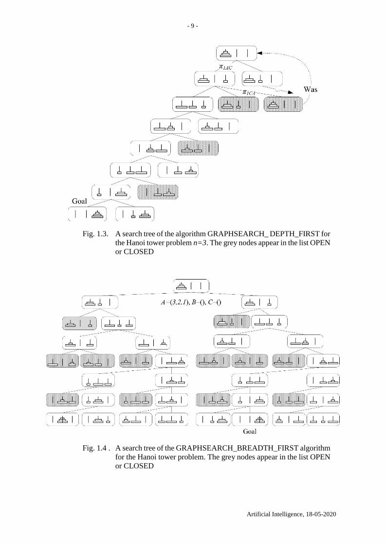
Further we discuss state transition in state transition graphs. Fig. 1.3 shows
GRAPHSEARCH-DEPTH-FIRST search tree for the Hanoi tower problem n=3.
- 9 -
Artificial Intelligence, 18-05-2020
Fig. 1.3. A search tree of the algorithm GRAPHSEARCH_ DEPTH_FIRST for
the Hanoi tower problem n=3. The grey nodes appear in the list OPEN
or CLOSED
Fig. 1.4 . A search tree of the GRAPHSEARCH_BREADTH_FIRST algorithm
for the Hanoi tower problem. The grey nodes appear in the list OPEN
or CLOSED
- 10 -
Artificial Intelligence, 18-05-2020
Exercise 1. The iterative Hanoi tower solution. The iterative algorithm for the Hanoi
tower problem is less well-known as the recursive one. First, we arrange the pegs in a circle, so
that clockwise we have A, B, C, and then A again. Following this, assuming we never move the
same disk twice in a row, there will always only be one disk that can be legally moved, and we
transfer it to the first peg it can occupy, moving in a clockwise direction, if n is even (2, 4, 6,…),
and counterclockwise, in n is odd (1, 3, 5,…). (See Brachman & Levesque (2004), “Knowledge
representation and reasoning”, p. 133–134, Exercise 2). Write a program.
Exercise 2. On the complexity of the Hanoi tower problem. Suppose one move takes 1
second. How many years will it take to solve the Hanoi tower problem for n=64?
Exercise 3. Monkey and banana problem. A monkey is in a room. Suspended from the
ceiling is a bunch of bananas, beyond the monkey’s reach. However, in the room there are also
a chair and a stick. The ceiling is just the right height so that a monkey standing on a chair could
knock the bananas down with the stick. The monkey knows how to move around, carry other
things around, reach for the bananas, and wave a stick in the air. What is the best sequence of
actions for the monkey? (https://en.wikipedia.org/wiki/Monkey_and_banana_problem)
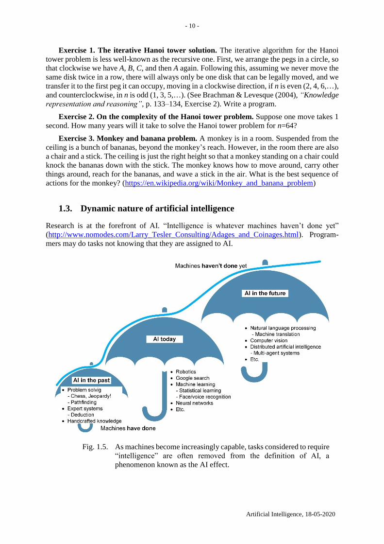
1.3. Dynamic nature of artificial intelligence
Research is at the forefront of AI. “Intelligence is whatever machines haven’t done yet”
(http://www.nomodes.com/Larry_Tesler_Consulting/Adages_and_Coinages.html). Program-
mers may do tasks not knowing that they are assigned to AI.
Fig. 1.5. As machines become increasingly capable, tasks considered to require
“intelligence” are often removed from the definition of AI, a
phenomenon known as the AI effect.
- 11 -
Artificial Intelligence, 18-05-2020
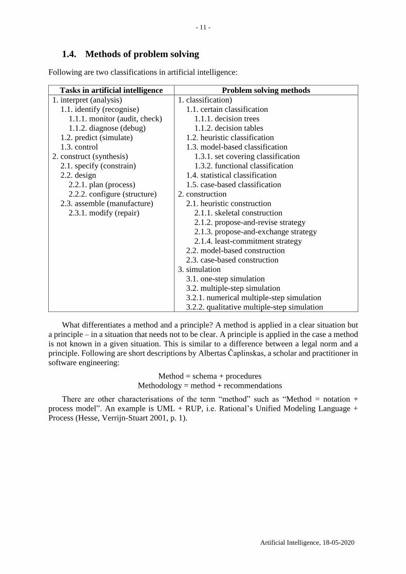
1.4. Methods of problem solving
Following are two classifications in artificial intelligence:
Tasks in artificial intelligence Problem solving methods
1. interpret (analysis)
1.1. identify (recognise)
1.1.1. monitor (audit, check)
1.1.2. diagnose (debug)
1.2. predict (simulate)
1.3. control
2. construct (synthesis)
2.1. specify (constrain)
2.2. design
2.2.1. plan (process)
2.2.2. configure (structure)
2.3. assemble (manufacture)
2.3.1. modify (repair)
1. classification)
1.1. certain classification
1.1.1. decision trees
1.1.2. decision tables
1.2. heuristic classification
1.3. model-based classification
1.3.1. set covering classification
1.3.2. functional classification
1.4. statistical classification
1.5. case-based classification
2. construction
2.1. heuristic construction
2.1.1. skeletal construction
2.1.2. propose-and-revise strategy
2.1.3. propose-and-exchange strategy
2.1.4. least-commitment strategy
2.2. model-based construction
2.3. case-based construction
3. simulation
3.1. one-step simulation
3.2. multiple-step simulation
3.2.1. numerical multiple-step simulation
3.2.2. qualitative multiple-step simulation
What differentiates a method and a principle? A method is applied in a clear situation but
a principle – in a situation that needs not to be clear. A principle is applied in the case a method
is not known in a given situation. This is similar to a difference between a legal norm and a
principle. Following are short descriptions by Albertas Čaplinskas, a scholar and practitioner in
software engineering:
Method = schema + procedures
Methodology = method + recommendations
There are other characterisations of the term “method” such as “Method = notation +
process model”. An example is UML + RUP, i.e. Rational’s Unified Modeling Language +
Process (Hesse, Verrijn-Stuart 2001, p. 1).
- 12 -
Artificial Intelligence, 18-05-2020
2. Artificial intelligence system as a production system
This chapter follows (Nilsson 1982, Section 1.1)
DEFINITION 2.1. A production system is a triple:
1. A global database (GDB);
2. A production (rule) set {1, 2,..., m};
3. A control system.
The basic production system algorithm for solving a problem such as the 8-puzzle, the
knight’s tour, the 8 queens puzzle, etc. can be written in nondeterministic form as follows:
procedure PRODUCTION
{1} DATA := initial GDB;
{2} until DATA will satisfy the termination condition, do
{3} begin
{4} select some rule, , in the set of rules that can be applied to DATA
{5} DATA := (DATA) {Result of applying to DATA} {6} end
The output is a sequence of productions i1, i2,...,in. This is a non-determinate
procedure. PRODUCTION performs depth-first search. The procedure is treated as a paradigm
of a control system. A meaning of the word “paradigm” can be found, for instance, in Oxford
English Dictionary, http://www.oed.com/: “A pattern or model, an exemplar; (also) a typical
instance of something, an example.”
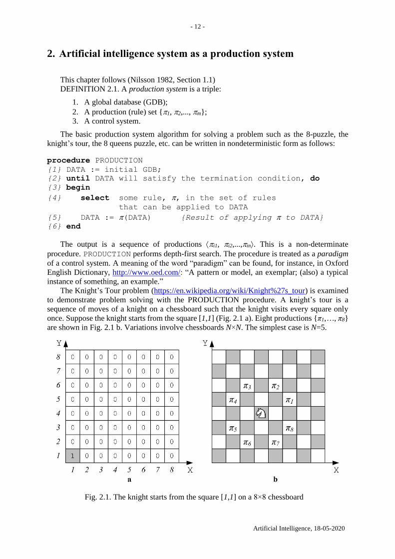
The Knight’s Tour problem (https://en.wikipedia.org/wiki/Knight%27s_tour) is examined
to demonstrate problem solving with the PRODUCTION procedure. A knight’s tour is a
sequence of moves of a knight on a chessboard such that the knight visits every square only
once. Suppose the knight starts from the square [1,1] (Fig. 2.1 a). Eight productions {π1,…, π8}
are shown in Fig. 2.1 b. Variations involve chessboards N×N. The simplest case is N=5.
Fig. 2.1. The knight starts from the square [1,1] on a 8×8 chessboard
- 13 -
Artificial Intelligence, 18-05-2020
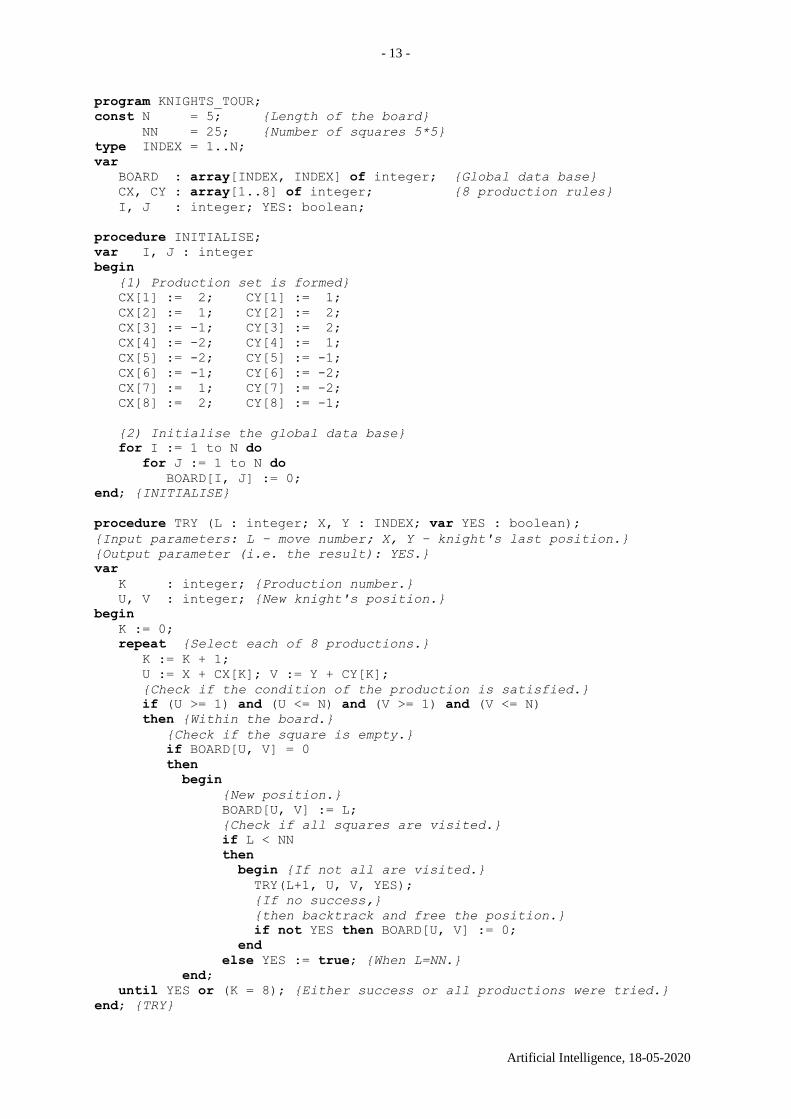
program KNIGHTS_TOUR;
const N = 5; {Length of the board}
NN = 25; {Number of squares 5*5}
type INDEX = 1..N;
var
BOARD : array[INDEX, INDEX] of integer; {Global data base}
CX, CY : array[1..8] of integer; {8 production rules}
I, J : integer; YES: boolean;
procedure INITIALISE;
var I, J : integer
begin
{1) Production set is formed}
CX[1] := 2; CY[1] := 1;
CX[2] := 1; CY[2] := 2;
CX[3] := -1; CY[3] := 2;
CX[4] := -2; CY[4] := 1;
CX[5] := -2; CY[5] := -1;
CX[6] := -1; CY[6] := -2;
CX[7] := 1; CY[7] := -2;
CX[8] := 2; CY[8] := -1;
{2) Initialise the global data base}
for I := 1 to N do
for J := 1 to N do
BOARD[I, J] := 0;
end; {INITIALISE}
procedure TRY (L : integer; X, Y : INDEX; var YES : boolean);
{Input parameters: L – move number; X, Y – knight's last position.}
{Output parameter (i.e. the result): YES.}
var
K : integer; {Production number.}
U, V : integer; {New knight's position.}
begin
K := 0;
repeat {Select each of 8 productions.}
K := K + 1;
U := X + CX[K]; V := Y + CY[K];
{Check if the condition of the production is satisfied.}
if (U >= 1) and (U <= N) and (V >= 1) and (V <= N)
then {Within the board.}
{Check if the square is empty.}
if BOARD[U, V] = 0
then
begin
{New position.}
BOARD[U, V] := L;
{Check if all squares are visited.}
if L < NN
then
begin {If not all are visited.}
TRY(L+1, U, V, YES);
{If no success,}
{then backtrack and free the position.}
if not YES then BOARD[U, V] := 0;
end
else YES := true; {When L=NN.}
end;
until YES or (K = 8); {Either success or all productions were tried.}
end; {TRY}
- 14 -
Artificial Intelligence, 18-05-2020
begin {Main program)}
{1. Initialise.}
INITIALISE; YES := false;
{2. Initial position [1,1].}
BOARD [1, 1] := 1;
{3. Make move no.2 from X=1 and Y=1 and obtain the answer YES.}
TRY(2, 1, 1, YES);
{4. If a solution found then print it.}
if YES then
for I := N downto 1 do
begin
for J := 1 to N do
write(BOARD[I,J]);
writeln;
end;
else writeln('Path does not exist.');
end.
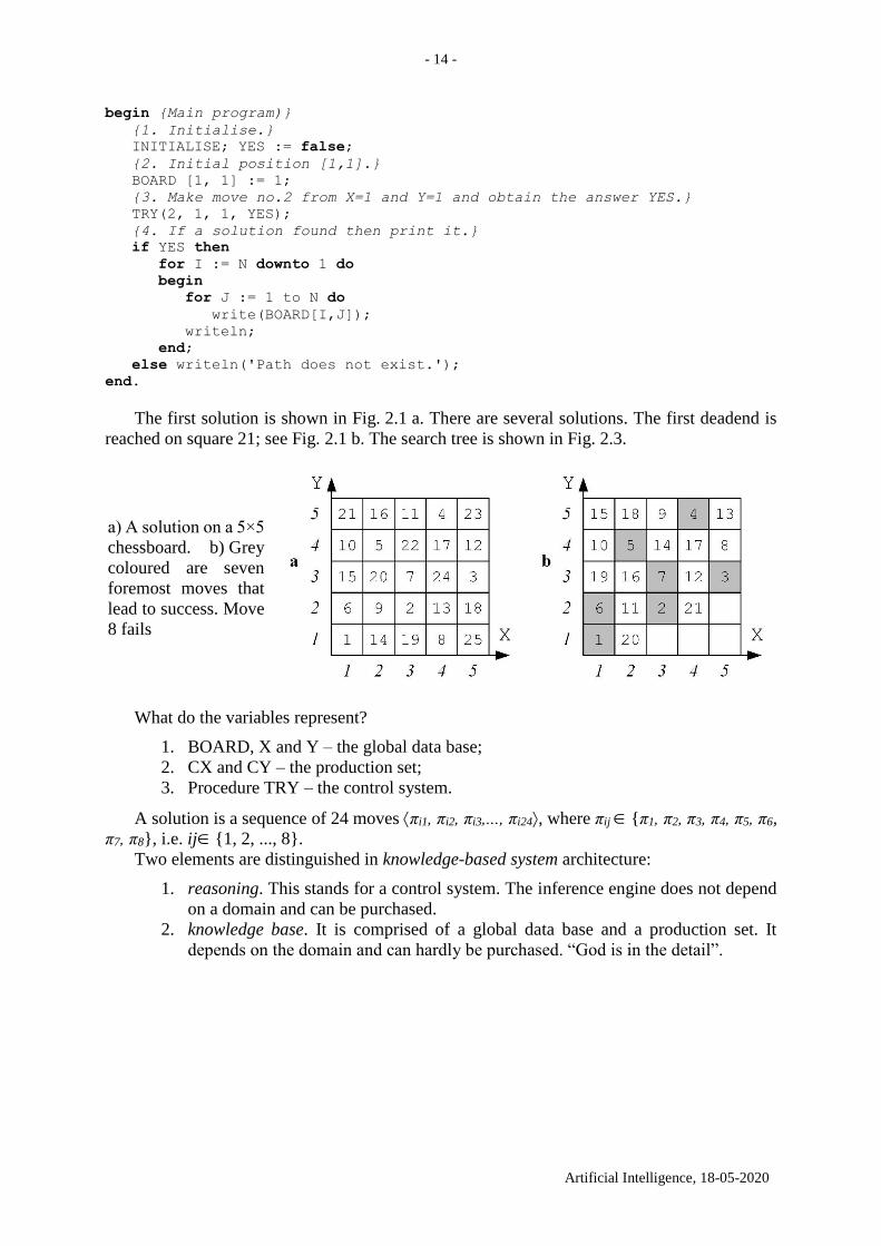
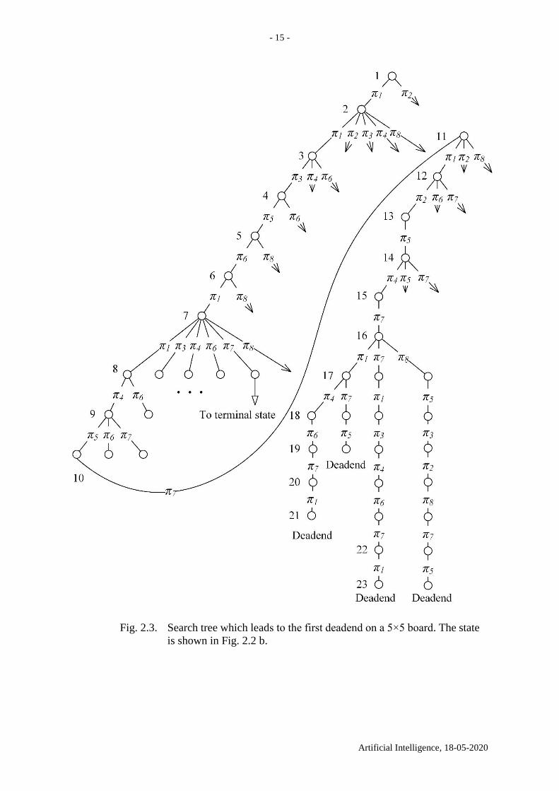
The first solution is shown in Fig. 2.1 a. There are several solutions. The first deadend is
reached on square 21; see Fig. 2.1 b. The search tree is shown in Fig. 2.3.
a) A solution on a 5×5
chessboard. b) Grey
coloured are seven
foremost moves that
lead to success. Move
8 fails
What do the variables represent?
1. BOARD, X and Y – the global data base;
2. CX and CY – the production set;
3. Procedure TRY – the control system.
A solution is a sequence of 24 moves πi1, πi2, πi3,..., πi24, where πij {π1, π2, π3, π4, π5, π6,
π7, π8}, i.e. ij{1, 2, ..., 8}.
Two elements are distinguished in knowledge-based system architecture:
1. reasoning. This stands for a control system. The inference engine does not depend
on a domain and can be purchased.
2. knowledge base. It is comprised of a global data base and a production set. It
depends on the domain and can hardly be purchased. “God is in the detail”.
- 15 -
Artificial Intelligence, 18-05-2020
Fig. 2.3. Search tree which leads to the first deadend on a 5×5 board. The state
is shown in Fig. 2.2 b.
- 16 -
Artificial Intelligence, 18-05-2020
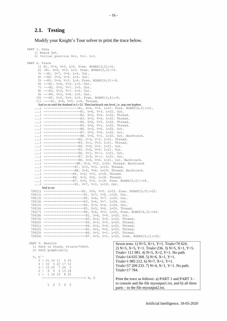
2.1. Testing
Modify your Knight’s Tour solver to print the trace below.
PART 1. Data
1) Board 5x5.
2) Initial position X=1, Y=1. L=1.
PART 2. Trace
1) R1. U=3, V=2. L=2. Free. BOARD[3,2]:=2.
2) -R1. U=5, V=3. L=3. Free. BOARD[5,3]:=3.
3) --R1. U=7, V=4. L=4. Out.
4) --R2. U=6, V=5. L=4. Out.
5) --R3. U=4, V=5. L=4. Free. BOARD[4,5]:=4.
6) ---R1. U=6, V=6. L=5. Out.
7) ---R2. U=5, V=7. L=5. Out.
8) ---R3. U=3, V=7. L=5. Out.
9) ---R4. U=2, V=6. L=5. Out.
10) ---R5. U=2, V=4. L=5. Free. BOARD[2,4]:=5.
11) ----R1. U=4, V=5. L=6. Thread.
And so on until the deadend at L=21. Then backtrack one level, i.e. pop one hyphen. ...) -------------------R1. U=4, V=2. L=21. Free. BOARD[4,2]:=21.
...) --------------------R1. U=6, V=3. L=22. Out.
...) --------------------R2. U=5, V=4. L=22. Thread.
...) --------------------R3. U=3, V=4. L=22. Thread.
...) --------------------R4. U=2, V=3. L=22. Thread.
...) --------------------R5. U=2, V=1. L=22. Thread.
...) --------------------R6. U=3, V=0. L=22. Out.
...) --------------------R7. U=5, V=0. L=22. Out.
...) --------------------R8. U=6, V=1. L=22. Out. Backtrack.
...) -------------------R2. U=3, V=3. L=21. Thread.
...) -------------------R3. U=1, V=3. L=21. Thread.
...) -------------------R4. U=0, V=2. L=21. Out.
...) -------------------R5. U=0, V=0. L=21. Out.
...) -------------------R6. U=1, V=-1. L=21. Out.
...) -------------------R7. U=3, V=-1. L=21. Out.
...) -------------------R8. U=4, V=0. L=21. Out. Backtrack.
...) ------------------R8. U=3, V=2. L=20. Thread. Backtrack
...) -----------------R7. U=3, V=3. L=19. Thread.
...) -----------------R8. U=4, V=4. L=19. Thread. Backtrack.
...) ----------------R5. U=2, V=3. L=18. Thread.
...) ----------------R6. U=3, V=2. L=18. Thread.
...) ----------------R7. U=5, V=2. L=18. Free. BOARD[5,2]:=18.
...) -----------------R1. U=7, V=3. L=19. Out.
And so on. 70611) ---------------------R1. U=5, V=5. L=23. Free. BOARD[5,5]:=23.
70612) ----------------------R1. U=7, V=6. L=24. Out.
70613) ----------------------R2. U=6, V=7. L=24. Out.
70614) ----------------------R3. U=4, V=7. L=24. Out.
70615) ----------------------R4. U=3, V=6. L=24. Out.
70616) ----------------------R5. U=3, V=4. L=24. Thread.
70617) ----------------------R6. U=4, V=3. L=24. Free. BOARD[4,3]:=24.
70618) -----------------------R1. U=6, V=4. L=25. Out.
70619) -----------------------R2. U=5, V=5. L=25. Thread.
70620) -----------------------R3. U=3, V=5. L=25. Thread.
70621) -----------------------R4. U=2, V=4. L=25. Thread.
70622) -----------------------R5. U=2, V=2. L=25. Thread.
70623) -----------------------R6. U=3, V=1. L=25. Thread.
70624) -----------------------R7. U=5, V=1. L=25. Free. BOARD[5,1]:=25.
PART 3. Results
1) Path is found. Trials=70624.
2) Path graphically
Y, V ^
5 | 21 16 11 4 23
4 | 10 5 22 17 12
3 | 15 20 7 24 3
2 | 6 9 2 13 18
1 | 1 14 19 8 25
-----------------------> X, U
1 2 3 4 5
Seven tests: 1) N=5, X=1, Y=1. Trials=70 624.
2) N=5, X=5, Y=1. Trials=236. 3) N=5, X=1, Y=5.
Trials= 111 981. 4) N=5, X=2, Y=1. No path.
Trials=14 635 368. 5) N=6, X=1, Y=1.
Trials=1 985 212. 6) N=7, X=1, Y=1.
Trials=57 209 233. 7) N=4, X=1, Y=1. No path.
Trials=17 784.
Print the trace as follows: a) PART 1 and PART 3 –
to console and the file myoutput1.txt, and b) all three
parts – to the file myoutput2.txt.
- 17 -
Artificial Intelligence, 18-05-2020
3. Control with backtracking and procedure BACKTRACK
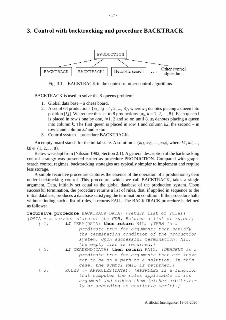
Fig. 3.1. BACKTRACK in the context of other control algorithms
BACKTRACK is used to solve the 8-queens problem:
1. Global data base – a chess board.
2. A set of 64 productions {πi,j, i,j = 1, 2, ..., 8}, where πi,j denotes placing a queen into
position [i,j]. We reduce this set to 8 productions {πk, k = 1, 2, ..., 8}. Each queen i
is placed in row i one by one, i=1, 2 and so on until 8. πk denotes placing a queen
into column k. The first queen is placed in row 1 and column k2, the second – in
row 2 and column k2 and so on.
3. Control system – procedure BACKTRACK.
An empty board stands for the initial state. A solution is πk1, πk2, , πk8, where k1, k2,,
k8 {1, 2,, 8}.
Below we adapt from (Nilsson 1982, Section 2.1). A general description of the backtracking
control strategy was presented earlier as procedure PRODUCTION. Compared with graph-
search control regimes, backtracking strategies are typically simpler to implement and require
less storage.
A simple recursive procedure captures the essence of the operation of a production system
under backtracking control. This procedure, which we call BACKTRACK, takes a single
argument, Data, initially set equal to the global database of the production system. Upon
successful termination, the procedure returns a list of rules, that, if applied in sequence to the
initial database, produces a database satisfying the termination condition. If the procedure halts
without finding such a list of rules, it returns FAIL. The BACKTRACK procedure is defined
as follows:
recursive procedure BACKTRACK(DATA) {return list of rules}
{DATA – a current state of the GDB. Returns a list of rules.}
{ 1} if TERM(DATA) then return NIL; {TERM is a
predicate true for arguments that satisfy
the termination condition of the production
system. Upon successful termination, NIL,
the empty list is returned.}
{ 2} if DEADEND(DATA) then return FAIL; {DEADEND is a
predicate true for arguments that are known
not to be on a path to a solution. In this
case, the symbol FAIL is returned.}
{ 3} RULES := APPRULES(DATA); {APPRULES is a function
that computes the rules applicable to its
argument and orders them (either arbitrari-
ly or according to heuristic merit).}
- 18 -
Artificial Intelligence, 18-05-2020
{ 4} LOOP: if NULL(RULES) then return FAIL;
{If there is no (more) rules to apply,
the procedure fails.}
{ 5} R := FIRST(RULES); {The best of the
applicable rules is selected.}
{ 6} RULES := TAIL(RULES); {The list of
applicable rules is diminished by
removing the one just selected.}
{ 7} RDATA := R(DATA); {Rule R is applied to
produce a new database.}
{ 8} PATH := BACKTRACK(RDATA); {Recursive call
on the new database.}
{ 9} if PATH = FAIL then goto LOOP; {If the re-
cursive call fails, try another rule.}
{10} return CONS(R, PATH); {Otherwise, pass the
successful list of rules up, by adding
R to the front of the list.}
end
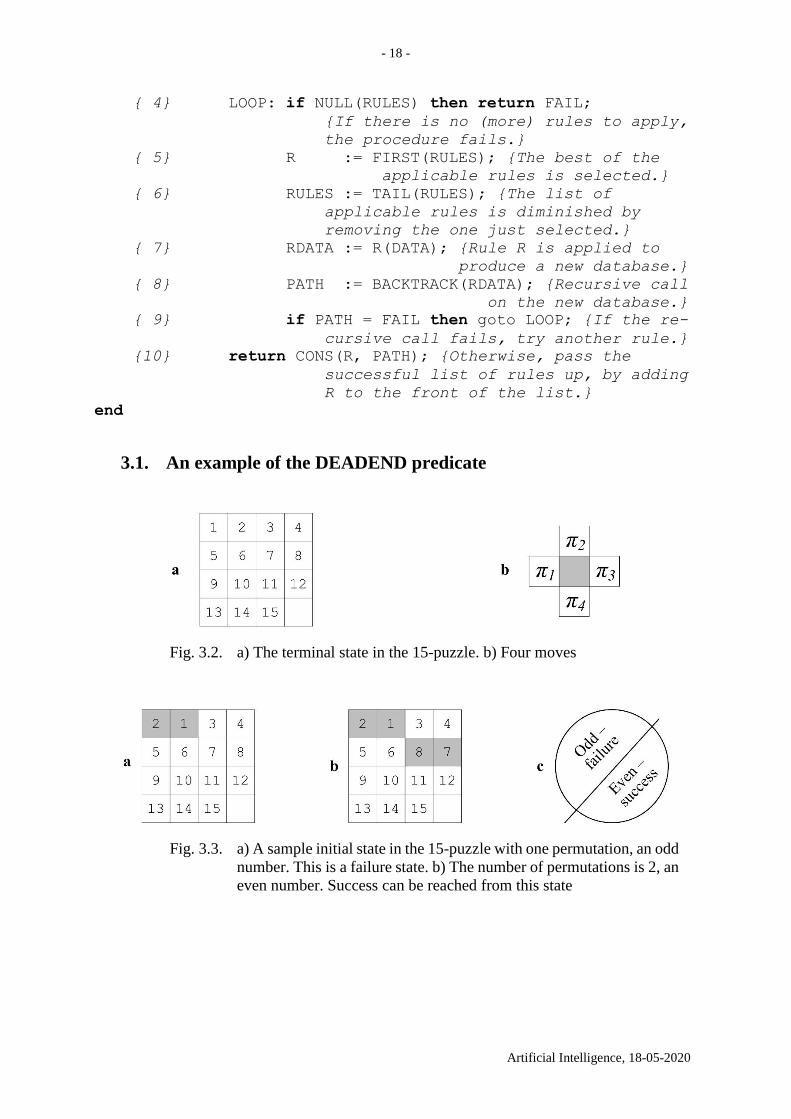
3.1. An example of the DEADEND predicate
Fig. 3.2. a) The terminal state in the 15-puzzle. b) Four moves
Fig. 3.3. a) A sample initial state in the 15-puzzle with one permutation, an odd
number. This is a failure state. b) The number of permutations is 2, an
even number. Success can be reached from this state
- 19 -
Artificial Intelligence, 18-05-2020
4. The 8-queens puzzle
Below we follow (Nilsson 1982, Section 2.1). Suppose the problem of placing 4 queens on
a 4×4 chessboard so that none can capture any other. For our global database, we use a 4×4
array with marked cells corresponding to squares occupied by queens. The terminal condition,
expressed by the predicate TERM, is satisfied for a database if and only if it has precisely 4
queen marks and the marks correspond to queens located so that they cannot capture each other.
There are many alternative formulations possible for the production rules. A useful one for
our purposes involves the following rule schema, for 1 ≤ i, j ≤ 4:
Rij Precondition:
i = 1: There are no marks in the array.
1 < i ≤ 4: There is a queen mark in row i – 1 of the array.
Effect: Puts a queen mark in row i, column j of the array.
Thus, the first queen mark added to the array must be in row 1, the second must be in row
2, etc.
To use the BACKRACK procedure to solve the 4-queens problem, we have still to specify
both the predicate DEADEND and an ordering relation for applicable rules. Suppose we
arbitrarily say that Rij is ahead of Rik in the ordering only when j < k. The predicate DEADEND
might be defined so that it is satisfied for databases where it is obvious that no solution is
possible; for example, certainly no solution is possible for any database containing a pair of
queen marks in mutually capturing positions. Altogether, the algorithm backtracks 22 times
before finding a solution; even the very first rule applied must ultimately be taken back (Nilsson
1982, p. 57–58). A search tree with 26 edges is shown in see Fig. 5.5.
To see an example of this multilevel backtracking phenomenon, consider using
BACKTRACK to solve the 8-queens problem. In this problem, we must place 8 queens on an
8×8 board so that none of them can capture any others. (Nilsson 1982, p. 60)
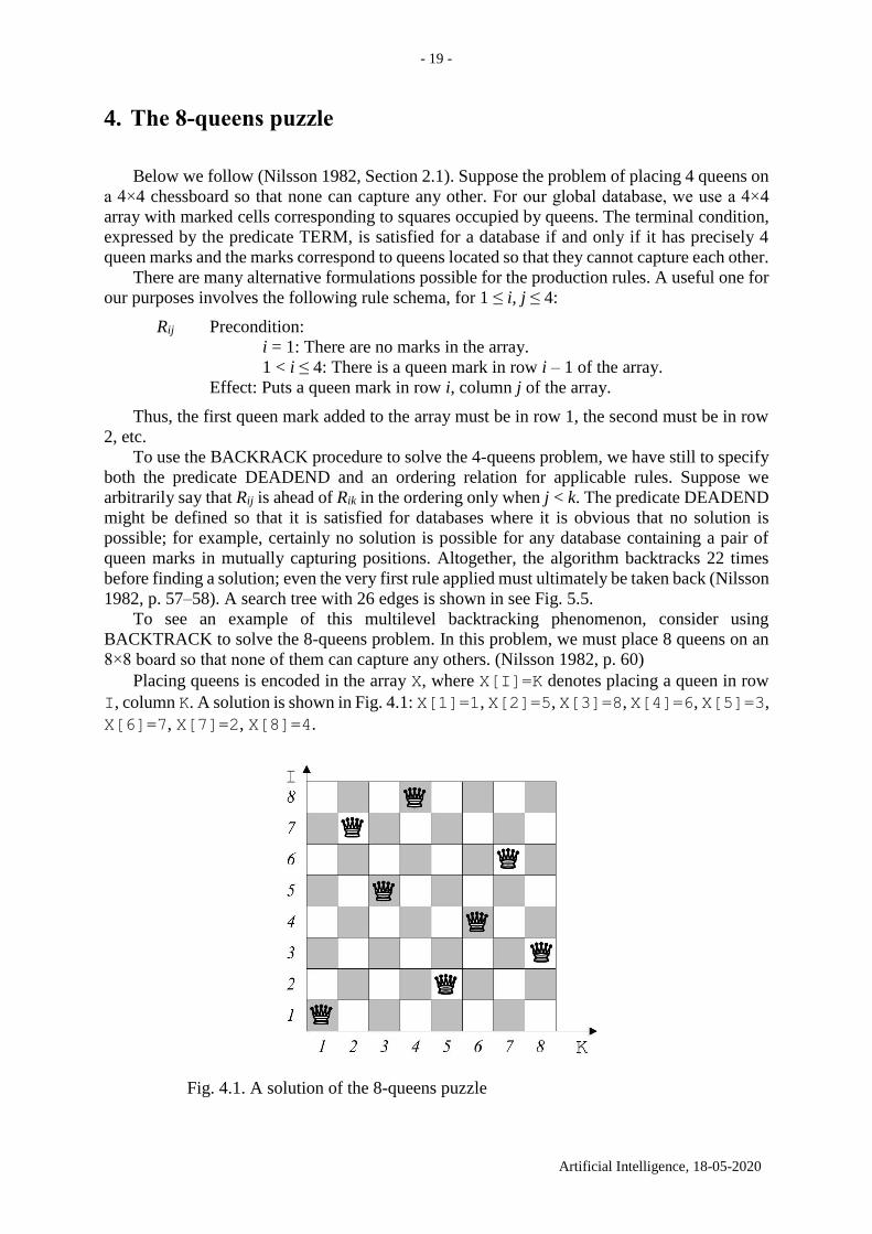
Placing queens is encoded in the array X, where X[I]=K denotes placing a queen in row
I, column K. A solution is shown in Fig. 4.1: X[1]=1, X[2]=5, X[3]=8, X[4]=6, X[5]=3,
X[6]=7, X[7]=2, X[8]=4.
Fig. 4.1. A solution of the 8-queens puzzle
- 20 -
Artificial Intelligence, 18-05-2020
A brute force algorithm searches among 8! = 876…21 = 40320 permutations. A solution
is as follows:
PATH=1, 5, 8, 6, 3, 7, 2, 4
Here the I-th element is X[I] , i.e. PATH[I] = X[I], where I = 1, 2, …, 8. There are N!
permutations in the case of an N×N board. As N grows, the factorial N! increases faster than all
polynomials and exponential functions, i.e. N! = 2N, where is a real number that depends
on N.
The program below follows (Dagienė, Grigas, Augutis, 1986); see also
https://en.wikipedia.org/wiki/Eight_queens_puzzle.
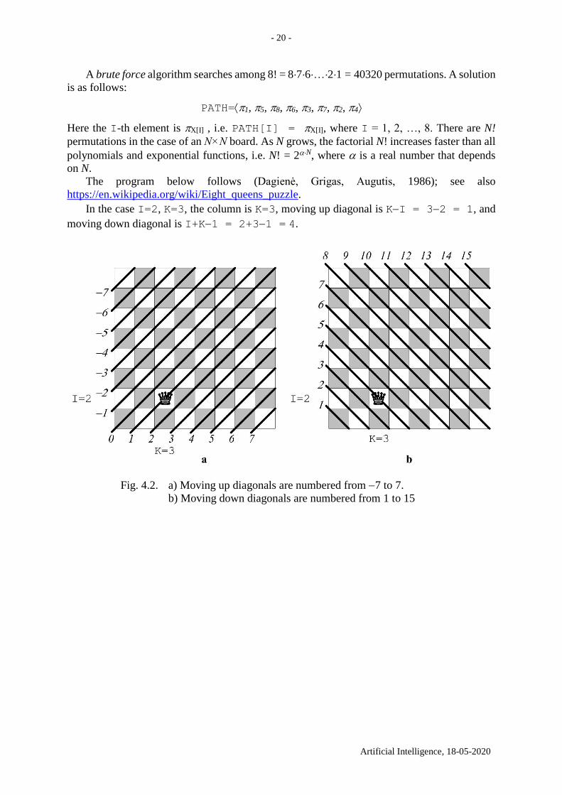
In the case I=2, K=3, the column is K=3, moving up diagonal is KI = 32 = 1, and
moving down diagonal is I+K1 = 2+31 = 4.
Fig. 4.2. a) Moving up diagonals are numbered from 7 to 7.
b) Moving down diagonals are numbered from 1 to 15
- 21 -
Artificial Intelligence, 18-05-2020
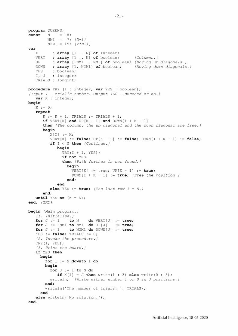
program QUEENS;
const N = 8;
NM1 = 7; {N-1}
N2M1 = 15; {2*N-1}
var
X : array [1 .. N] of integer;
VERT : array [1 .. N] of boolean; {Columns.}
UP : array [-NM1 .. NM1] of boolean; {Moving up diagonals.}
DOWN : array [1..N2M1] of boolean; {Moving down diagonals.}
YES : boolean;
I, J : integer;
TRIALS : longint;
procedure TRY (I : integer; var YES : boolean);
{Input I – trial‘s number. Output YES – succeed or no.}
var K : integer;
begin
K := 0;
repeat
K := K + 1; TRIALS := TRIALS + 1;
if VERT[K] and UP[K - I] and DOWN[I + K - 1]
then {The column, the up diagonal and the down diagonal are free.}
begin
X[I] := K;
VERT[K] := false; UP[K - I] := false; DOWN[I + K - 1] := false;
if I < N then {Continue.}
begin
TRY(I + 1, YES);
if not YES
then {Path further is not found.}
begin
VERT[K] := true; UP[K - I] := true;
DOWN[I + K - 1] := true; {Free the position.}
end;
end
else YES := true; {The last row I = N.}
end;
until YES or (K = N);
end; {TRY}
begin {Main program.}
{1. Initialise.}
for J := 1 to N do VERT[J] := true;
for J := -NM1 to NM1 do UP[J] := true;
for J := 1 to N2M1 do DOWN[J] := true;
YES := false; TRIALS := 0;
{2. Invoke the procedure.}
TRY(1, YES);
{3. Print the board.}
if YES then
begin
for I := N downto 1 do
begin
for J := 1 to N do
if X[I] = J then write(1 : 3) else write(0 : 3);
writeln; {Write either number 1 or 0 in 3 positions.}
end;
writeln('The number of trials: ', TRIALS);
end
else writeln('No solution.');
end.
- 22 -
Artificial Intelligence, 18-05-2020
5. Heuristic
A heuristic is a rule of thumb; see (Russell, Norvig, 2003, p. 94). The term “heuristic” see
Oxford English Dictionary, http://www.oed.com/:
adjective a. Serving to find out or discover…
c. Under an ‘heuristic’ programming procedure the computer searches through a
number of possible solutions at each stage of the programme, it evaluates a ‘good’
solution for this stage and then proceeds to the next stage. Essentially heuristic
programming is similar to the problem solving techniques by trial and error
methods which we use in everyday life. (1964 T. W. McRae)
noun b. A process that may solve a given problem, but offers no guarantees of doing so, is
called a heuristic for that problem. Ibid. For conciseness, we will use ‘heuristic’
as a noun synonymous with ‘heuristic process’. (1957 A. Newell et al.)
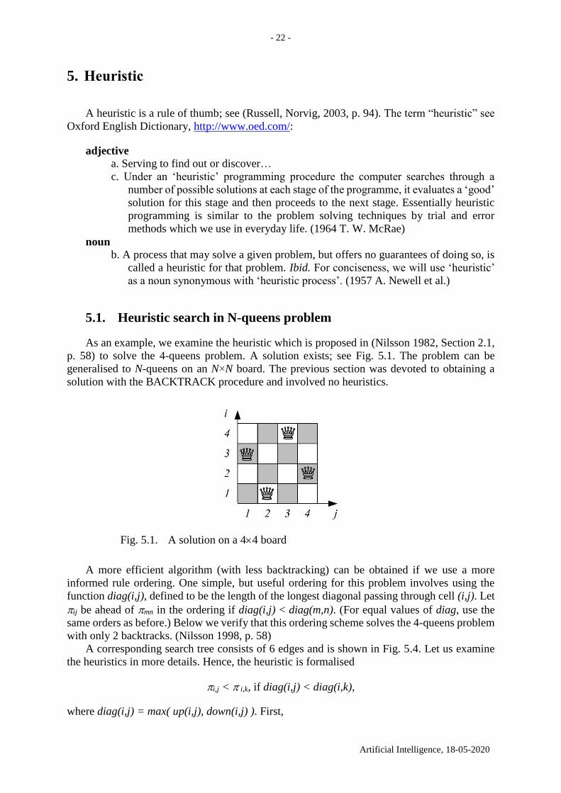
5.1. Heuristic search in N-queens problem
As an example, we examine the heuristic which is proposed in (Nilsson 1982, Section 2.1,
p. 58) to solve the 4-queens problem. A solution exists; see Fig. 5.1. The problem can be
generalised to N-queens on an N×N board. The previous section was devoted to obtaining a
solution with the BACKTRACK procedure and involved no heuristics.
Fig. 5.1. A solution on a 44 board
A more efficient algorithm (with less backtracking) can be obtained if we use a more
informed rule ordering. One simple, but useful ordering for this problem involves using the
function diag(i,j), defined to be the length of the longest diagonal passing through cell (i,j). Let
ij be ahead of mn in the ordering if diag(i,j) < diag(m,n). (For equal values of diag, use the
same orders as before.) Below we verify that this ordering scheme solves the 4-queens problem
with only 2 backtracks. (Nilsson 1998, p. 58)
A corresponding search tree consists of 6 edges and is shown in Fig. 5.4. Let us examine
the heuristics in more details. Hence, the heuristic is formalised
i,j < i,k, if diag(i,j) < diag(i,k),
where diag(i,j) = max( up(i,j), down(i,j) ). First,
- 23 -
Artificial Intelligence, 18-05-2020
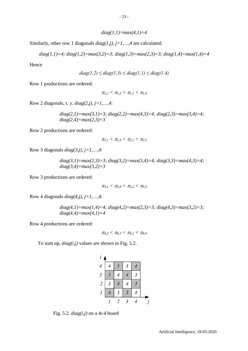
diag(1,1)=max(4,1)=4
Similarly, other row 1 diagonals diag(1,j), j=1,…,4 are calculated:
diag(1,1)=4; diag(1,2)=max(3,2)=3; diag(1,3)=max(2,3)=3; diag(1,4)=max(1,4)=4
Hence
diag(1,2) ≤ diag(1,3) ≤ diag(1,1) ≤ diag(1,4)
Row 1 productions are ordered:
1,2 < 1,3 < 1,1 < 1,4
Row 2 diagonals, t. y. diag(2,j), j=1,…,4:
diag(2,1)=max(3,1)=3; diag(2,2)=max(4,3)=4; diag(2,3)=max(3,4)=4;
diag(2,4)=max(2,3)=3
Row 2 productions are ordered:
2,1 < 2,4 < 2,2 < 2,3
Row 3 diagonals diag(3,j), j=1,…,4:
diag(3,1)=max(2,3)=3; diag(3,2)=max(3,4)=4; diag(3,3)=max(4,3)=4;
diag(3,4)=max(3,2)=3
Row 3 productions are ordered:
3,1 < 3,4 < 3,2 < 3,3
Row 4 diagonals diag(4,j), j=1,…,4:
diag(4,1)=max(1,4)=4; diag(4,2)=max(2,3)=3; diag(4,3)=max(3,2)=3;
diag(4,4)=max(4,1)=4
Row 4 productions are ordered:
4,2 < 4,3 < 4,1 < 4,4
To sum up, diag(i,j) values are shown in Fig. 5.2.
Fig. 5.2. diag(i,j) on a 44 board
- 24 -
Artificial Intelligence, 18-05-2020
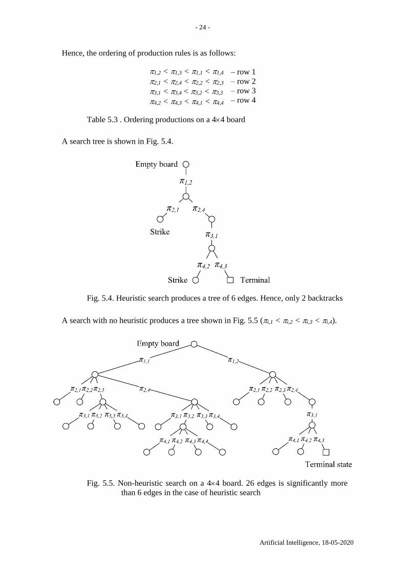
Hence, the ordering of production rules is as follows:
1,2 < 1,3 < 1,1 < 1,4
2,1 < 2,4 < 2,2 < 2,3
3,1 < 3,4 < 3,2 < 3,3
4,2 < 4,3 < 4,1 < 4,4
– row 1
– row 2
– row 3
– row 4
Table 5.3 . Ordering productions on a 44 board
A search tree is shown in Fig. 5.4.
Fig. 5.4. Heuristic search produces a tree of 6 edges. Hence, only 2 backtracks
A search with no heuristic produces a tree shown in Fig. 5.5 (i,1 < i,2 < i,3 < i,4).
Fig. 5.5. Non-heuristic search on a 44 board. 26 edges is significantly more
than 6 edges in the case of heuristic search
- 25 -
Artificial Intelligence, 18-05-2020
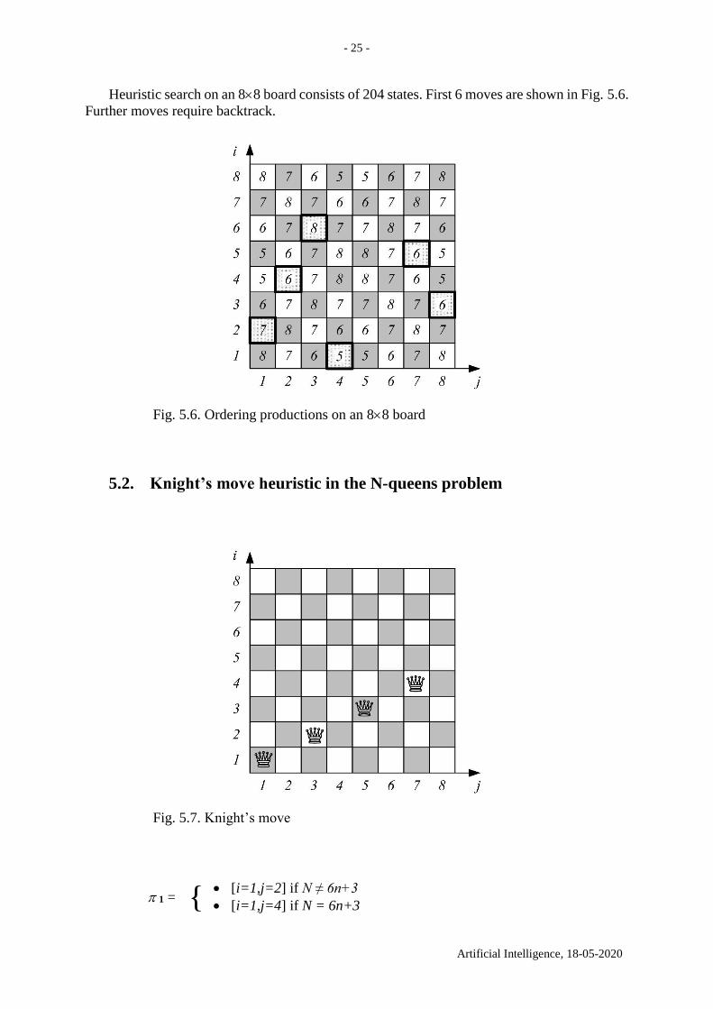
Heuristic search on an 88 board consists of 204 states. First 6 moves are shown in Fig. 5.6.
Further moves require backtrack.
Fig. 5.6. Ordering productions on an 88 board
5.2. Knight’s move heuristic in the N-queens problem
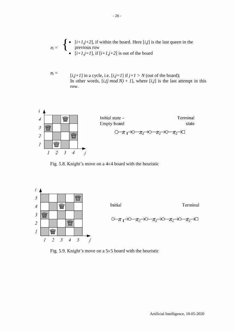
Fig. 5.7. Knight’s move
1 = { [i=1,j=2] if N ≠ 6n+3
[i=1,j=4] if N = 6n+3
- 26 -
Artificial Intelligence, 18-05-2020
ž = {
[i+1,j+2], if within the board. Here [i,j] is the last queen in the
previous row
[i+1,j=1], if [i+1,j+2] is out of the board
k =
[i,j+1] in a cycle, i.e. [i,j=1] if j+1 > N (out of the board);
In other words, [i,(j mod N) + 1], where [i,j] is the last attempt in this
row.
Fig. 5.8. Knight’s move on a 44 board with the heuristic
Fig. 5.9. Knight’s move on a 55 board with the heuristic
- 27 -
Artificial Intelligence, 18-05-2020
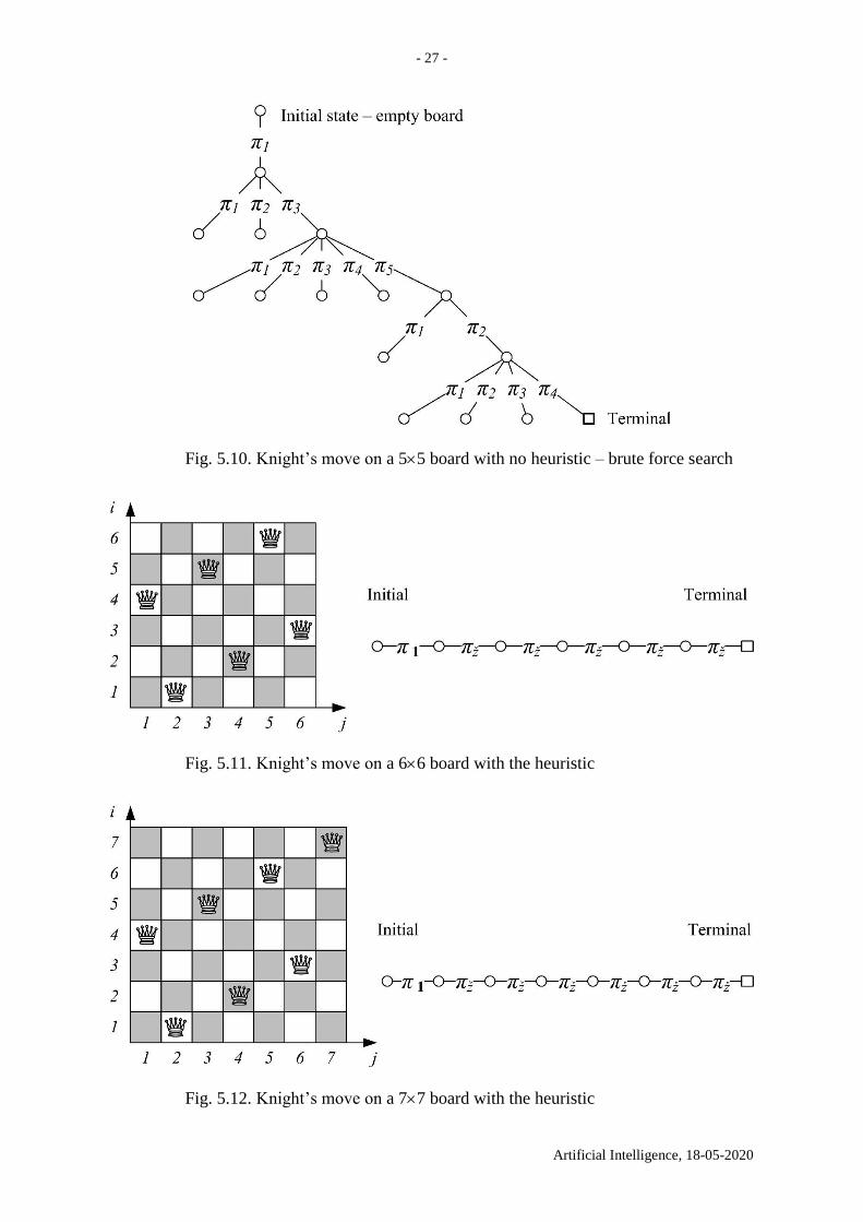
Fig. 5.10. Knight’s move on a 55 board with no heuristic – brute force search
Fig. 5.11. Knight’s move on a 66 board with the heuristic
Fig. 5.12. Knight’s move on a 77 board with the heuristic
- 28 -
Artificial Intelligence, 18-05-2020
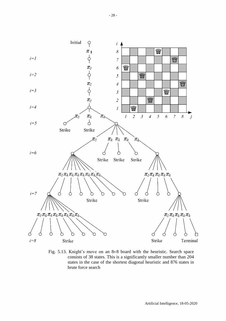
Fig. 5.13. Knight’s move on an 88 board with the heuristic. Search space
consists of 38 states. This is a significantly smaller number than 204
states in the case of the shortest diagonal heuristic and 876 states in
brute force search
- 29 -
Artificial Intelligence, 18-05-2020
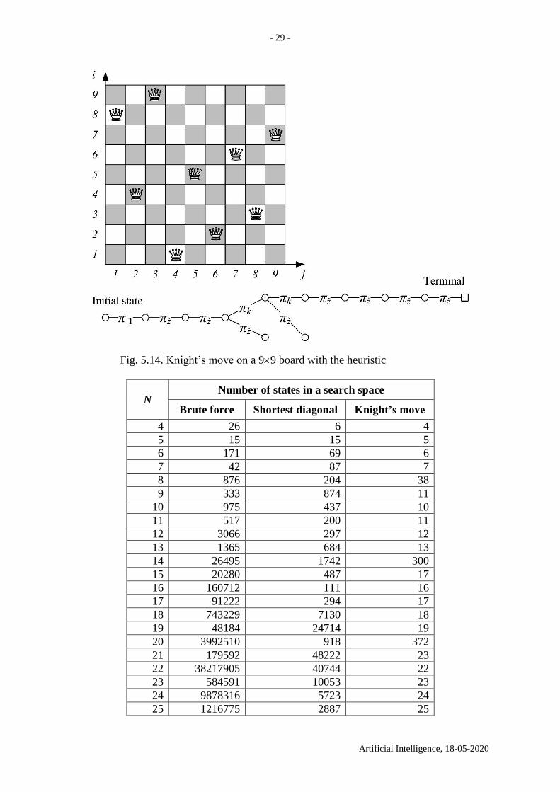
Fig. 5.14. Knight’s move on a 99 board with the heuristic
N Number of states in a search space
Brute force Shortest diagonal Knight’s move
4 26 6 4
5 15 15 5
6 171 69 6
7 42 87 7
8 876 204 38
9 333 874 11
10 975 437 10
11 517 200 11
12 3066 297 12
13 1365 684 13
14 26495 1742 300
15 20280 487 17
16 160712 111 16
17 91222 294 17
18 743229 7130 18
19 48184 24714 19
20 3992510 918 372
21 179592 48222 23
22 38217905 40744 22
23 584591 10053 23
24 9878316 5723 24
25 1216775 2887 25
- 30 -
Artificial Intelligence, 18-05-2020
26 10339849 265187 2196
27 12263400 986476 29
28 84175966 2602283 28
29 44434525 1261296 29
30 1692888135 52601 30
31 Many 1850449 31
32 Many 2804692 2866
33 Many 2582396 35
34 Many 35784 34
35 Many 110473 35
36 Many 19605979 36
37 Many 135980 37
38 Many 642244758 30532
39 Many 193745 41
40 Many 4685041 40
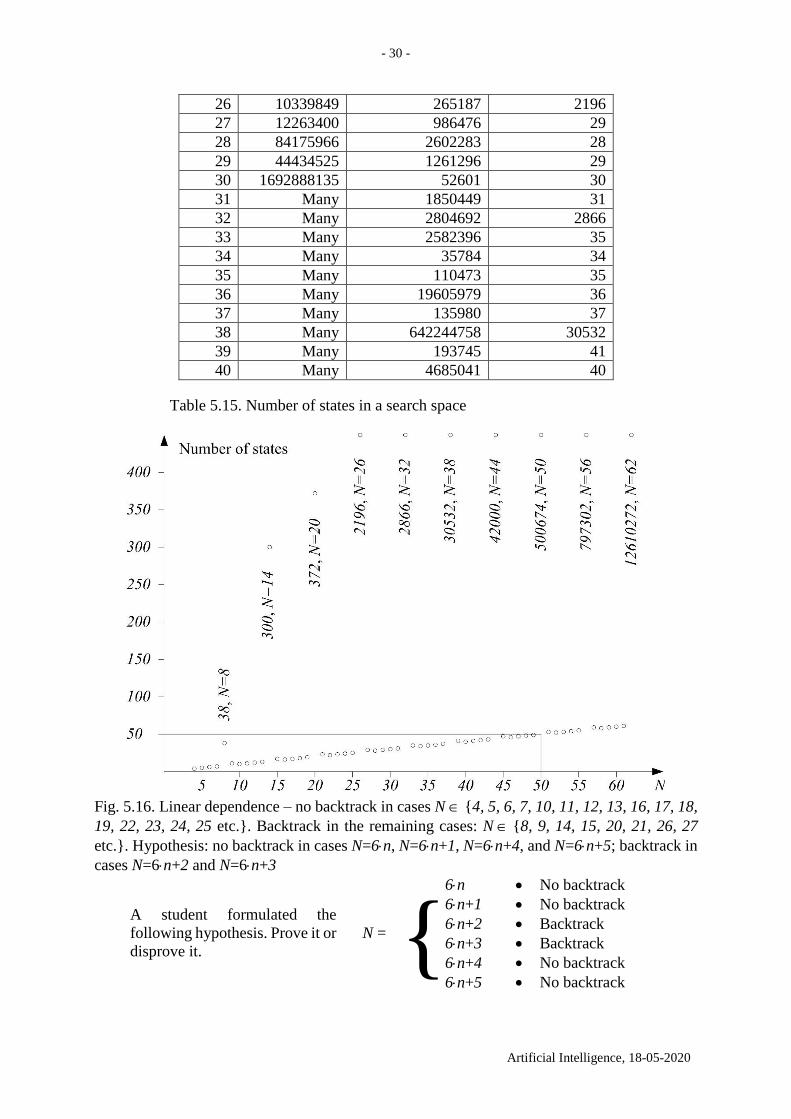
Table 5.15. Number of states in a search space
Fig. 5.16. Linear dependence – no backtrack in cases N {4, 5, 6, 7, 10, 11, 12, 13, 16, 17, 18,
19, 22, 23, 24, 25 etc.}. Backtrack in the remaining cases: N {8, 9, 14, 15, 20, 21, 26, 27
etc.}. Hypothesis: no backtrack in cases N=6n, N=6n+1, N=6n+4, and N=6n+5; backtrack in
cases N=6n+2 and N=6n+3
A student formulated the
following hypothesis. Prove it or
disprove it.
N = {
6n
6n+1
6n+2
6n+3
6n+4
6n+5
No backtrack
No backtrack
Backtrack
Backtrack
No backtrack
No backtrack
- 31 -
Artificial Intelligence, 18-05-2020
6. BACKTRACK1 – a cycle-avoiding algorithm
Below we follow [Nilsson 1982 Section 2.1, p. 56–61]. Procedure BACKTRACK may
never terminate; it may generate new nonterminal databases indefinitely or it may cycle.
(Cycling is demonstrated with a LABYRINTH depth-first search program in the next section.)
Both of these cases can be arbitrarily prevented by imposing a depth bound on the recursion.
Cycling can be more straightforwardly prevented by maintaining a list of the databases
produced so far and by checking new ones to see that they do not match any on the list.
Therefore we need a slightly more complex algorithm to avoid cycles. All databases on a
path back to the initial one must be checked to insure that none are revisited. In order to
implement this backtracking strategy as a recursive procedure, the entire chain of databases
must be an argument of the procedure. Again, practical implementations of AI backtracking
production systems use various techniques to avoid the need for explicitly listing all of these
databases in their entirety.
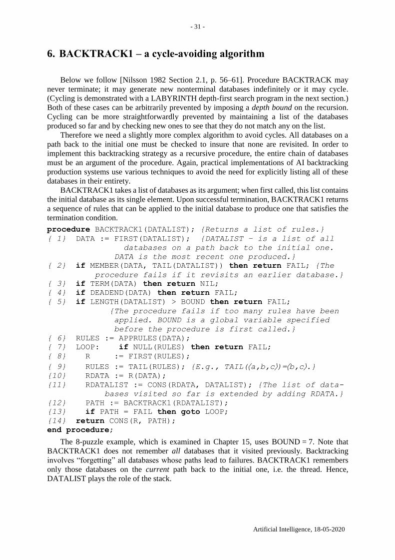
BACKTRACK1 takes a list of databases as its argument; when first called, this list contains
the initial database as its single element. Upon successful termination, BACKTRACK1 returns
a sequence of rules that can be applied to the initial database to produce one that satisfies the
termination condition.
procedure BACKTRACK1(DATALIST); {Returns a list of rules.}
{ 1} DATA := FIRST(DATALIST); {DATALIST – is a list of all
databases on a path back to the initial one.
DATA is the most recent one produced.}
{ 2} if MEMBER(DATA, TAIL(DATALIST)) then return FAIL; {The
procedure fails if it revisits an earlier database.}
{ 3} if TERM(DATA) then return NIL;
{ 4} if DEADEND(DATA) then return FAIL;
{ 5} if LENGTH(DATALIST) > BOUND then return FAIL;
{The procedure fails if too many rules have been
applied. BOUND is a global variable specified
before the procedure is first called.}
{ 6} RULES := APPRULES(DATA);
{ 7} LOOP: if NULL(RULES) then return FAIL;
{ 8} R := FIRST(RULES);
{ 9} RULES := TAIL(RULES); {E.g., TAIL(a,b,c)=b,c.} {10} RDATA := R(DATA);
{11} RDATALIST := CONS(RDATA, DATALIST); {The list of data-
bases visited so far is extended by adding RDATA.}
{12} PATH := BACKTRACK1(RDATALIST);
{13} if PATH = FAIL then goto LOOP;
{14} return CONS(R, PATH);
end procedure;
The 8-puzzle example, which is examined in Chapter 15, uses BOUND = 7. Note that
BACKTRACK1 does not remember all databases that it visited previously. Backtracking
involves “forgetting” all databases whose paths lead to failures. BACKTRACK1 remembers
only those databases on the current path back to the initial one, i.e. the thread. Hence,
DATALIST plays the role of the stack.
- 32 -
Artificial Intelligence, 18-05-2020
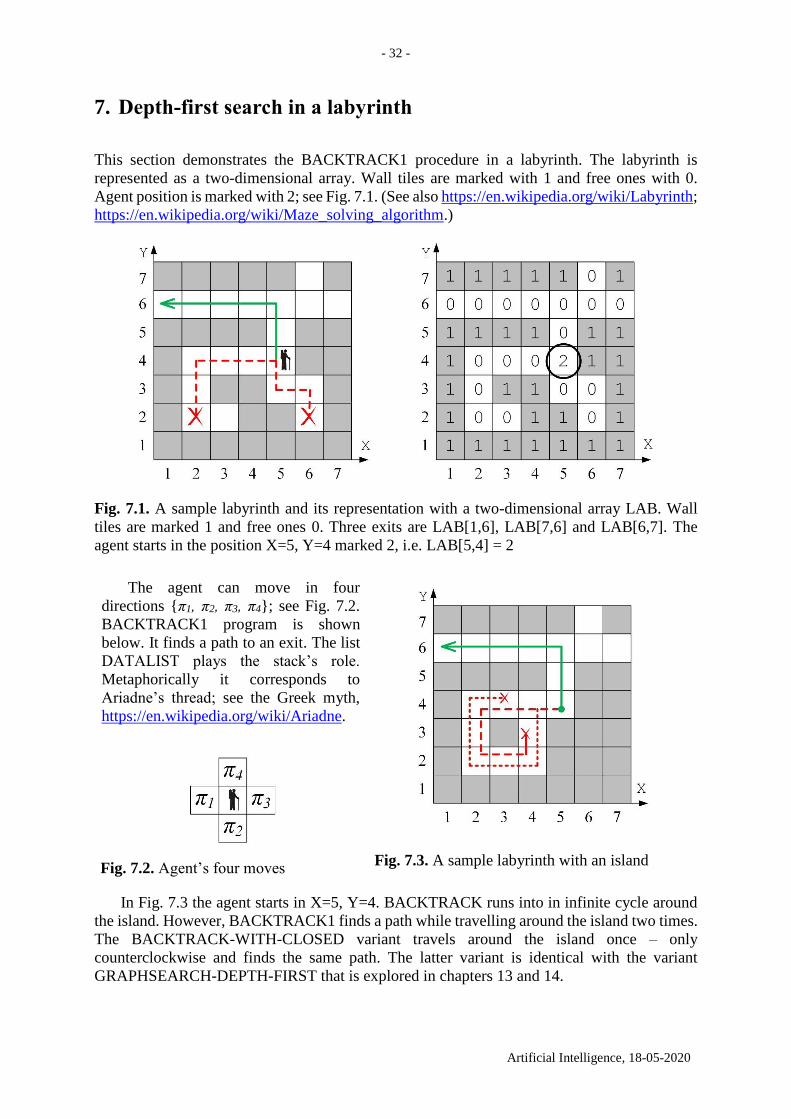
7. Depth-first search in a labyrinth
This section demonstrates the BACKTRACK1 procedure in a labyrinth. The labyrinth is
represented as a two-dimensional array. Wall tiles are marked with 1 and free ones with 0.
Agent position is marked with 2; see Fig. 7.1. (See also https://en.wikipedia.org/wiki/Labyrinth;
https://en.wikipedia.org/wiki/Maze_solving_algorithm.)
Fig. 7.1. A sample labyrinth and its representation with a two-dimensional array LAB. Wall
tiles are marked 1 and free ones 0. Three exits are LAB[1,6], LAB[7,6] and LAB[6,7]. The
agent starts in the position X=5, Y=4 marked 2, i.e. LAB[5,4] = 2
The agent can move in four
directions {π1, π2, π3, π4}; see Fig. 7.2.
BACKTRACK1 program is shown
below. It finds a path to an exit. The list
DATALIST plays the stack’s role.
Metaphorically it corresponds to
Ariadne’s thread; see the Greek myth,
https://en.wikipedia.org/wiki/Ariadne.
Fig. 7.2. Agent’s four moves
Fig. 7.3. A sample labyrinth with an island
In Fig. 7.3 the agent starts in X=5, Y=4. BACKTRACK runs into in infinite cycle around
the island. However, BACKTRACK1 finds a path while travelling around the island two times.
The BACKTRACK-WITH-CLOSED variant travels around the island once – only
counterclockwise and finds the same path. The latter variant is identical with the variant
GRAPHSEARCH-DEPTH-FIRST that is explored in chapters 13 and 14.
- 33 -
Artificial Intelligence, 18-05-2020
program LABYRINTH; {BACKTRACK1, i.e. depth-first, no infinite cycle.}
const M = 7; N = 7; {Dimensions.}
var LAB : array[1..M, 1..N] of integer; {Labyrinth.}
CX, CY : array[1..4] of integer; {4 production – shifts in X and Y.}
L, {Move’s number. Starts from 2. Visited positions are marked.}
X, Y, {Agent’s initial position.}
I, J, {Loop variables.}
TRIAL : integer; {Number of trials. To compare effectiveness.}
YES : boolean; {True – success, false – failure.}
procedure TRY(X, Y : integer; var YES : boolean);
var K, {The number of a production rule.}
U, V : integer; {Agent’s new position.}
begin {TRY}
{K1} if (X = 1) or (X = M) or (Y = 1) or (Y = N)
then YES := true {TERM(DATA} = true on the boarder.}
else
begin K := 0;
{K2} repeat K := K + 1; {Next rule. Loop over production rules.}
{K3} U := X + CX[K]; V := Y + CY[K]; {Agent’s new position.}
{K4} if LAB[U, V] = 0 {If a cell is free.}
then
begin TRIAL := TRIAL + 1; {Number of trials.}
{K5} L := L + 1; LAB[U,V] := L;{Marking the cell.}
{K6} TRY(U, V, YES); {Recursive call.}
if not YES {If failure}
{K7} then begin
{K8} LAB[U,V] := -1; {then mark. (0 in case of BACKTRACK).}
L := L - 1;
end;
end;
until YES or (K = 4);
end;
end; {TRY}
begin {Main program.}
{1. Reading the labyrinth.}
for J := 1 to N do
begin
for I := 1 to M do read(LAB[I,J]);
readln;
end;
{2. Reading agent’s position.}
read(X, Y); L := 2; LAB[X,Y] := L;
{3. Forming four production rules.}
CX[1] := -1; CY[1] := 0; {Go West. 4 }
CX[2] := 0; CY[2] := -1; {Go South. 1 * 3 }
CX[3] := 1; CY[3] := 0; {Go East. 2 }
CX[4] := 0; CY[4] := 1; {Go North. }
{4. Initialising variables.}
YES := false; TRIAL := 0;
{5. Invoking the BACKTRACK1 procedure.}
TRY(X, Y, YES);
if YES
then writeln('Path exists'); {Please also print the path found.}
else writeln('Path does not exist'); {No paths exist.}
end.
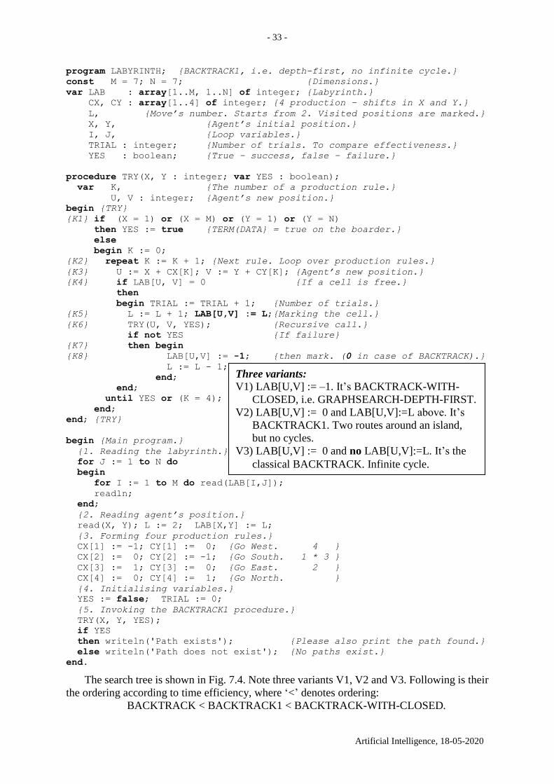
The search tree is shown in Fig. 7.4. Note three variants V1, V2 and V3. Following is their
the ordering according to time efficiency, where ‘<’ denotes ordering:
BACKTRACK < BACKTRACK1 < BACKTRACK-WITH-CLOSED.
Three variants:
V1) LAB[U,V] := –1. It’s BACKTRACK-WITH-
CLOSED, i.e. GRAPHSEARCH-DEPTH-FIRST.
V2) LAB[U,V] := 0 and LAB[U,V]:=L above. It’s
BACKTRACK1. Two routes around an island,
but no cycles.
V3) LAB[U,V] := 0 and no LAB[U,V]:=L. It’s the
classical BACKTRACK. Infinite cycle.
- 34 -
Artificial Intelligence, 18-05-2020
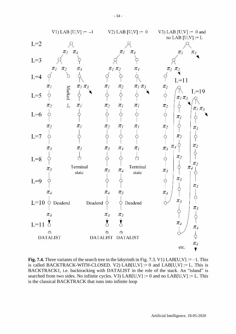
Fig. 7.4. Three variants of the search tree in the labyrinth in Fig. 7.3. V1) LAB[U,V] := –1. This
is called BACKTRACK-WITH-CLOSED. V2) LAB[U,V] := 0 and LAB[U,V] := L. This is
BACKTRACK1, i.e. backtracking with DATALIST in the role of the stack. An “island” is
searched from two sides. No infinite cycles. V3) LAB[U,V] := 0 and no LAB[U,V] := L. This
is the classical BACKTRACK that runs into infinite loop
- 35 -
Artificial Intelligence, 18-05-2020
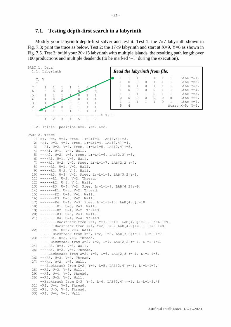
7.1. Testing depth-first search in a labyrinth
Modify your labyrinth depth-first solver and test it. Test 1: the 77 labyrinth shown in
Fig. 7.3; print the trace as below. Test 2: the 179 labyrinth and start at X=9, Y=6 as shown in
Fig. 7.5. Test 3: build your 2015 labyrinth with multiple islands, the resulting path length over
100 productions and multiple deadends (to be marked ‘–1’ during the execution).
PART 1. Data
1.1. Labyrinth
Y, V
^
7 | 1 1 1 1 1 0 1
6 | 0 0 0 0 0 0 0
5 | 1 1 1 1 0 1 1
4 | 1 0 0 0 0 1 1
3 | 1 0 1 0 1 1 1
2 | 1 0 0 0 1 1 1
1 | 1 1 1 1 1 1 1
-------------------------------> X, U
1 2 3 4 5 6 7
1.2. Initial position X=5, Y=4. L=2.
PART 2. Trace
1) R1. U=4, V=4. Free. L:=L+1=3. LAB[4,4]:=3.
2) -R1. U=3, V=4. Free. L:=L+1=4. LAB[3,4]:=4.
3) --R1. U=2, V=4. Free. L:=L+1=5. LAB[2,4]:=5.
4) ---R1. U=1, V=4. Wall.
5) ---R2. U=2, V=3. Free. L:=L+1=6. LAB[2,3]:=6.
6) ----R1. U=1, V=3. Wall.
7) ----R2. U=2, V=2. Free. L:=L+1=7. LAB[2,2]:=7.
8) -----R1. U=1, V=2. Wall.
9) -----R2. U=2, V=1. Wall.
10) -----R3. U=3, V=2. Free. L:=L+1=8. LAB[3,2]:=8.
11) ------R1. U=2, V=2. Thread.
12) ------R2. U=3, V=1. Wall.
13) ------R3. U=4, V=2. Free. L:=L+1=9. LAB[4,2]:=9.
14) -------R1. U=3, V=2. Thread.
15) -------R2. U=4, V=1. Wall.
16) -------R3. U=5, V=2. Wall.
17) -------R4. U=4, V=3. Free. L:=L+1=10. LAB[4,3]:=10.
18) --------R1. U=3, V=3. Wall.
19) --------R2. U=4, V=2. Thread.
20) --------R3. U=5, V=3. Wall.
21) --------R4. U=4, V=4. Thread.
--------Backtrack from X=4, Y=3, L=10. LAB[4,3]:=-1. L:=L-1=9.
-------Backtrack from X=4, Y=2, L=9. LAB[4,2]:=-1. L:=L-1=8.
22) ------R4. U=3, V=3. Wall.
------Backtrack from X=3, Y=2, L=8. LAB[3,2]:=-1. L:=L-1=7.
23) -----R4. U=2, V=3. Thread.
-----Backtrack from X=2, Y=2, L=7. LAB[2,2]:=-1. L:=L-1=6.
24) ----R3. U=3, V=3. Wall.
25) ----R4. U=2, V=4. Thread.
----Backtrack from X=2, Y=3, L=6. LAB[2,3]:=-1. L:=L-1=5.
26) ---R3. U=3, V=4. Thread.
27) ---R4. U=2, V=5. Wall.
---Backtrack from X=2, Y=4, L=5. LAB[2,4]:=-1. L:=L-1=4.
28) --R2. U=3, V=3. Wall.
29) --R3. U=4, V=4. Thread.
30) --R4. U=3, V=5. Wall.
--Backtrack from X=3, Y=4, L=4. LAB[3,4]:=-1. L:=L-1=3.*8
31) -R2. U=4, V=3. Thread.
32) -R3. U=5, V=4. Thread.
33) -R4. U=4, V=5. Wall.
Read the labyrinth from file:
1 1 1 1 1 1 1 Line Y=1.
1 0 0 0 1 1 1 Line Y=2.
1 0 1 0 1 1 1 Line Y=3.
1 0 0 0 0 1 1 Line Y=4.
1 1 1 1 0 1 1 Line Y=5.
0 0 0 0 0 0 0 Line Y=6.
1 1 1 1 1 0 1 Line Y=7.
5 4 Start X=5, Y=4.
- 36 -
Artificial Intelligence, 18-05-2020
-Backtrack from X=4, Y=4, L=3. LAB[4,4]:=-1. L:=L-1=2.
34) R2. U=5, V=3. Wall.
35) R3. U=6, V=4. Wall.
36) R4. U=5, V=5. Free. L:=L+1=3. LAB[5,5]:=3.
37) -R1. U=4, V=5. Wall.
38) -R2. U=5, V=4. Thread.
39) -R3. U=6, V=5. Wall.
40) -R4. U=5, V=6. Free. L:=L+1=4. LAB[5,6]:=4.
41) --R1. U=4, V=6. Free. L:=L+1=5. LAB[4,6]:=5.
42) ---R1. U=3, V=6. Free. L:=L+1=6. LAB[3,6]:=6.
43) ----R1. U=2, V=6. Free. L:=L+1=7. LAB[2,6]:=7.
44) -----R1. U=1, V=6. Free. L:=L+1=8. LAB[1,6]:=8. Terminal.
PART 3. Results
3.1. Path is found.
3.2. Path graphically:
Y, V
7 | 1 1 1 1 1 0 1
6 | 8 7 6 5 4 0 0
5 | 1 1 1 1 3 1 1
4 | 1 -1 -1 -1 2 1 1
3 | 1 -1 1 -1 1 1 1
2 | 1 -1 -1 -1 1 1 1
1 | 1 1 1 1 1 1 1
-------------------------------> X, U
1 2 3 4 5 6 7
3.3. Rules: R4, R4, R1, R1, R1, R1.
3.4. Nodes: [X=5,Y=4], [X=5,Y=5], [X=5,Y=6], [X=4,Y=6], [X=3,Y=6], [X=2,Y=6],
[X=1,Y=6].
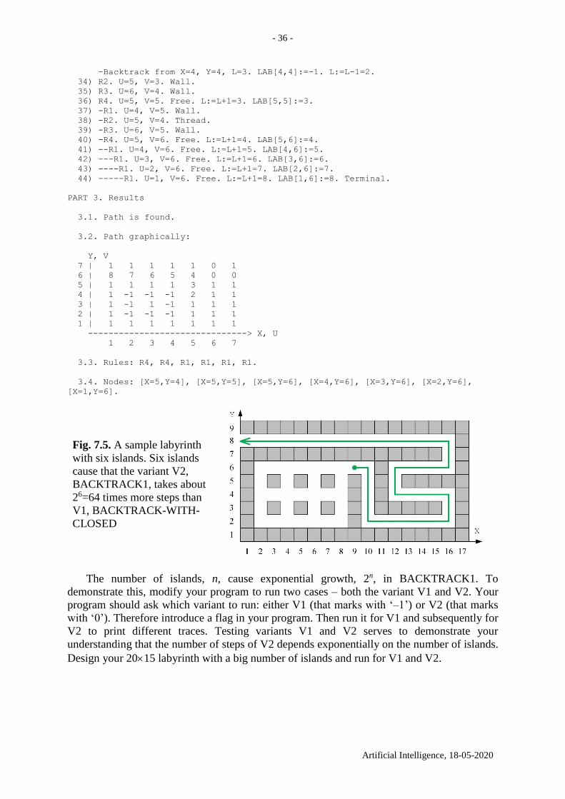
Fig. 7.5. A sample labyrinth
with six islands. Six islands
cause that the variant V2,
BACKTRACK1, takes about
26=64 times more steps than
V1, BACKTRACK-WITH-
CLOSED
The number of islands, n, cause exponential growth, 2n, in BACKTRACK1. To
demonstrate this, modify your program to run two cases – both the variant V1 and V2. Your
program should ask which variant to run: either V1 (that marks with ‘–1’) or V2 (that marks
with ‘0’). Therefore introduce a flag in your program. Then run it for V1 and subsequently for
V2 to print different traces. Testing variants V1 and V2 serves to demonstrate your
understanding that the number of steps of V2 depends exponentially on the number of islands.
Design your 2015 labyrinth with a big number of islands and run for V1 and V2.
- 37 -
Artificial Intelligence, 18-05-2020
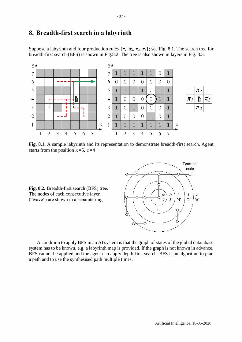
8. Breadth-first search in a labyrinth
Suppose a labyrinth and four production rules {π1, π2, π3, π4}; see Fig. 8.1. The search tree for
breadth-first search (BFS) is shown in Fig.8.2. The tree is also shown in layers in Fig. 8.3.
Fig. 8.1. A sample labyrinth and its representation to demonstrate breadth-first search. Agent
starts from the position X=5, Y=4
Fig. 8.2. Breadth-first search (BFS) tree.
The nodes of each consecutive layer
(“wave”) are shown in a separate ring
A condition to apply BFS in an AI system is that the graph of states of the global datatabase
system has to be known, e.g. a labyrinth map is provided. If the graph is not known in advance,
BFS cannot be applied and the agent can apply depth-first search. BFS is an algorithm to plan
a path and to use the synthesised path multiple times.
- 38 -
Artificial Intelligence, 18-05-2020
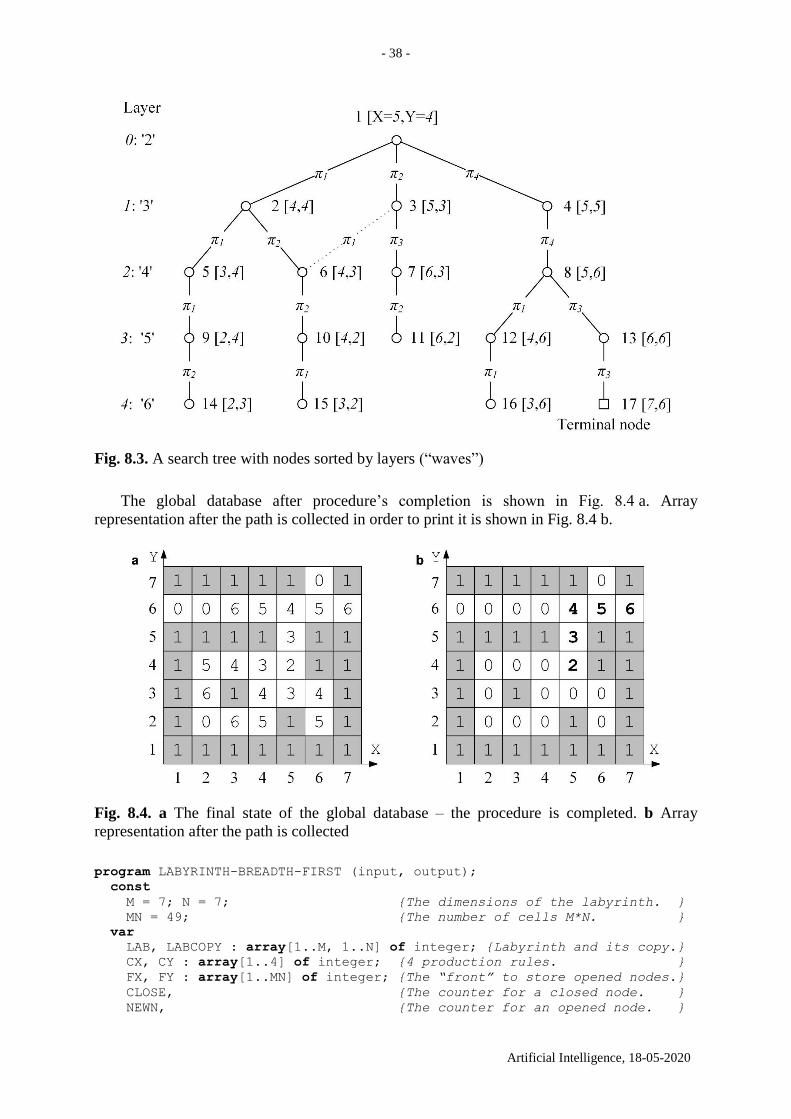
Fig. 8.3. A search tree with nodes sorted by layers (“waves”)
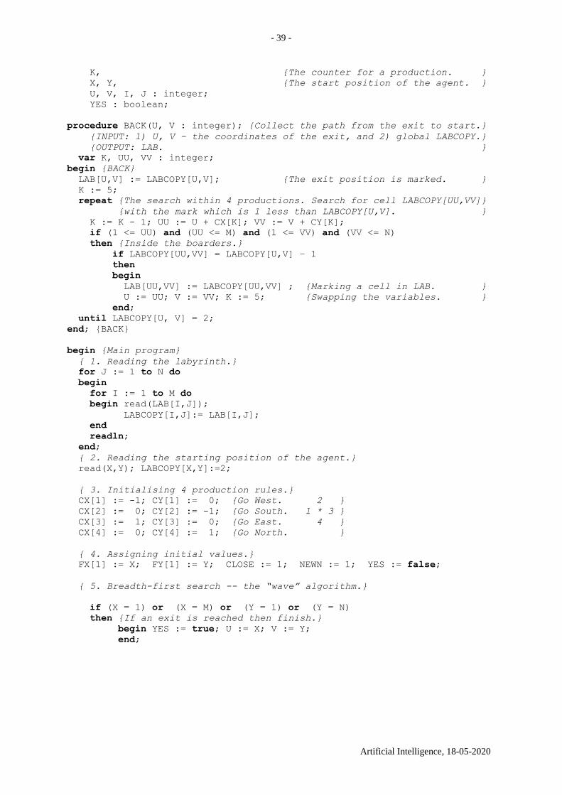
The global database after procedure’s completion is shown in Fig. 8.4 a. Array
representation after the path is collected in order to print it is shown in Fig. 8.4 b.
Fig. 8.4. a The final state of the global database – the procedure is completed. b Array
representation after the path is collected
program LABYRINTH-BREADTH-FIRST (input, output);
const
M = 7; N = 7; {The dimensions of the labyrinth. }
MN = 49; {The number of cells M*N. }
var
LAB, LABCOPY : array[1..M, 1..N] of integer; {Labyrinth and its copy.}
CX, CY : array[1..4] of integer; {4 production rules. }
FX, FY : array[1..MN] of integer; {The “front” to store opened nodes.}
CLOSE, {The counter for a closed node. }
NEWN, {The counter for an opened node. }
- 39 -
Artificial Intelligence, 18-05-2020
K, {The counter for a production. }
X, Y, {The start position of the agent. }
U, V, I, J : integer;
YES : boolean;
procedure BACK(U, V : integer); {Collect the path from the exit to start.}
{INPUT: 1) U, V – the coordinates of the exit, and 2) global LABCOPY.}
{OUTPUT: LAB. }
var K, UU, VV : integer;
begin {BACK}
LAB[U,V] := LABCOPY[U,V]; {The exit position is marked. }
K := 5;
repeat {The search within 4 productions. Search for cell LABCOPY[UU,VV]}
{with the mark which is 1 less than LABCOPY[U,V]. }
K := K - 1; UU := U + CX[K]; VV := V + CY[K];
if (1 <= UU) and (UU <= M) and (1 <= VV) and (VV <= N)
then {Inside the boarders.}
if LABCOPY[UU,VV] = LABCOPY[U,V] – 1
then
begin
LAB[UU,VV] := LABCOPY[UU,VV] ; {Marking a cell in LAB. }
U := UU; V := VV; K := 5; {Swapping the variables. }
end;
until LABCOPY[U, V] = 2;
end; {BACK}
begin {Main program}
{ 1. Reading the labyrinth.}
for J := 1 to N do
begin
for I := 1 to M do
begin read(LAB[I,J]);
LABCOPY[I,J]:= LAB[I,J];
end
readln;
end;
{ 2. Reading the starting position of the agent.}
read(X,Y); LABCOPY[X,Y]:=2;
{ 3. Initialising 4 production rules.}
CX[1] := -1; CY[1] := 0; {Go West. 2 }
CX[2] := 0; CY[2] := -1; {Go South. 1 * 3 }
CX[3] := 1; CY[3] := 0; {Go East. 4 }
CX[4] := 0; CY[4] := 1; {Go North. }
{ 4. Assigning initial values.}
FX[1] := X; FY[1] := Y; CLOSE := 1; NEWN := 1; YES := false;
{ 5. Breadth-first search -- the “wave” algorithm.}
if (X = 1) or (X = M) or (Y = 1) or (Y = N)
then {If an exit is reached then finish.}
begin YES := true; U := X; V := Y;
end;
- 40 -
Artificial Intelligence, 18-05-2020
if (X > 1) and (X < M) and (Y > 1) and (Y < N)
then
repeat {The loop through the nodes.}
X := FX[CLOSE]; Y := FY[CLOSE]; {Coordinates of node to be closed.}
K := 0;
repeat {The loop trough 4 production rules.}
K := K + 1; U := X + CX[K]; V := Y + CY[K];
if LABCOPY[U, V] = 0 {The cell is free.}
then begin
LABCOPY[U,V] := LABCOPY[X,Y] + 1; {New wave’s number.}
if (U = 1) or (U = M) or (V = 1) or (V = N) {Boarder. }
then YES := true; {Success. Here BACK(U,V) could be called.}
else begin {Placing a newly opened node into front’s end. }
NEWN := NEWN + 1; FX[NEWN] := U; FY[NEWN] := V;
end;
end;
until (K = 4) or YES; {Each of 4 productions is checked or success.}
CLOSE := CLOSE + 1; {Next node will be closed.}
until (CLOSE > NEWN) or YES;
{ 6. Printing the path found.}
if YES
then begin
writeln('The path exists.');
BACK(U,V); {Collecting the path.}
{ Here a procedure should be called to print the path.}
end
else writeln('No path.');
end.
The solution is π4, π4, π3, π3. During program execution, the coordinates of newly opened
nodes are placed into the arrays FX and FY. This is shown in Table. 8.5.
Table 8.5. The frontier arrays FX[i] and FY[i] during the execution
I 1 2 3 4 5 6 7 8 9 10 11 12 13 14 15 16 17
Wave '2' '3' '3' '3' '4' '4' '4' '4' '5' '5' '5' '5' '5' '6' '6' '6' '6'
FX 5 4 5 5 3 4 6 5 2 4 6 4 6 2 3 3 7
FY 4 4 3 5 4 3 3 6 4 2 2 6 6 3 2 6 6 CLOSE:=1
CLOSE=1
CLOSE=1
CLOSE=1
CLOSE=2
CLOSE=2
CLOSE=3
CLOSE=4
CLOSE=5
CLOSE=6
CLOSE=7
CLOSE=8
CLOSE=8
CLOSE=9
CLOSE=10
CLOSE=12
CLOSE=13
Stop
NEWN:2
NEWN:3
NEWN:4
NEWN:5
NEWN:6
NEWN:7
NEWN:8
NEWN:9
NEWN:10
NEWN:11
NEWN:12
NEWN:13
NEWN:14
NEWN:15
NEWN:16
NEWN:17
Breadth-first search visits the neighbour vertices before visiting the child vertices, and a
queue is used. Depth-first search visits the child vertices before visiting the sibling vertices. A
stack (often the program’s call stack via recursion) is generally used when implementing the
algorithm; see Wikipedia, https://en.wikipedia.org/wiki/Breadth-first_search,
https://en.wikipedia.org/wiki/Depth-first_search, and also
https://en.wikipedia.org/wiki/Graph_traversal.
- 41 -
Artificial Intelligence, 18-05-2020
8.1. Testing breadth-first search in a labyrinth
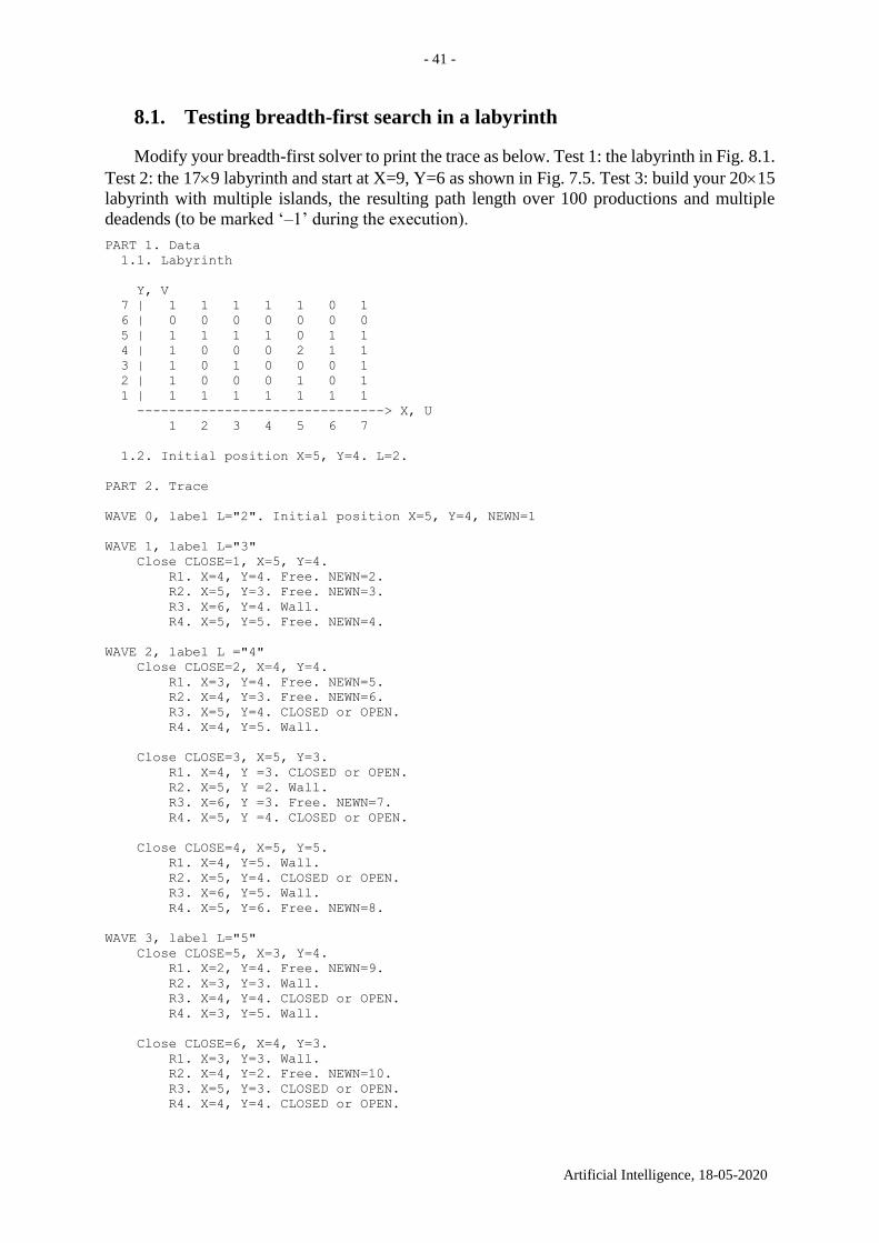
Modify your breadth-first solver to print the trace as below. Test 1: the labyrinth in Fig. 8.1.
Test 2: the 179 labyrinth and start at X=9, Y=6 as shown in Fig. 7.5. Test 3: build your 2015
labyrinth with multiple islands, the resulting path length over 100 productions and multiple
deadends (to be marked ‘–1’ during the execution).
PART 1. Data
1.1. Labyrinth
Y, V
7 | 1 1 1 1 1 0 1
6 | 0 0 0 0 0 0 0
5 | 1 1 1 1 0 1 1
4 | 1 0 0 0 2 1 1
3 | 1 0 1 0 0 0 1
2 | 1 0 0 0 1 0 1
1 | 1 1 1 1 1 1 1
-------------------------------> X, U
1 2 3 4 5 6 7
1.2. Initial position X=5, Y=4. L=2.
PART 2. Trace
WAVE 0, label L="2". Initial position X=5, Y=4, NEWN=1
WAVE 1, label L="3"
Close CLOSE=1, X=5, Y=4.
R1. X=4, Y=4. Free. NEWN=2.
R2. X=5, Y=3. Free. NEWN=3.
R3. X=6, Y=4. Wall.
R4. X=5, Y=5. Free. NEWN=4.
WAVE 2, label L ="4"
Close CLOSE=2, X=4, Y=4.
R1. X=3, Y=4. Free. NEWN=5.
R2. X=4, Y=3. Free. NEWN=6.
R3. X=5, Y=4. CLOSED or OPEN.
R4. X=4, Y=5. Wall.
Close CLOSE=3, X=5, Y=3.
R1. X=4, Y =3. CLOSED or OPEN.
R2. X=5, Y =2. Wall.
R3. X=6, Y =3. Free. NEWN=7.
R4. X=5, Y =4. CLOSED or OPEN.
Close CLOSE=4, X=5, Y=5.
R1. X=4, Y=5. Wall.
R2. X=5, Y=4. CLOSED or OPEN.
R3. X=6, Y=5. Wall.
R4. X=5, Y=6. Free. NEWN=8.
WAVE 3, label L="5"
Close CLOSE=5, X=3, Y=4.
R1. X=2, Y=4. Free. NEWN=9.
R2. X=3, Y=3. Wall.
R3. X=4, Y=4. CLOSED or OPEN.
R4. X=3, Y=5. Wall.
Close CLOSE=6, X=4, Y=3.
R1. X=3, Y=3. Wall.
R2. X=4, Y=2. Free. NEWN=10.
R3. X=5, Y=3. CLOSED or OPEN.
R4. X=4, Y=4. CLOSED or OPEN.
- 42 -
Artificial Intelligence, 18-05-2020
Close CLOSE=7, X=6, Y=3.
R1. X=5, Y=3. CLOSED or OPEN.
R2. X=6, Y=2. Free. NEWN=11.
R3. X=7, Y=3. Wall.
R4. X=6, Y=4. Wall.
Close CLOSE=8, X=5, Y=6.
R1. X=4, Y=6. Free. NEWN=12.
R2. X=5, Y=5. CLOSED or OPEN.
R3. X=6, Y=6. Free. NEWN=13.
R4. X=5, Y=7. Wall.
WAVE 4, label L="6"
Close CLOSE=9, X=2, Y=4.
R1. X=1, Y=4. Wall.
R2. X=2, Y=3. Free. NEWN=14.
R3. X=3, Y=4. CLOSED or OPEN.
R4. X=2, Y=5. Wall.
Close CLOSE=10, X=4, Y=2.
R1. X=3, Y=2. Free. NEWN=15.
R2. X=4, Y=1. Wall.
R3. X=5, Y=2. Wall.
R4. X=4, Y=3. CLOSED or OPEN.
Close CLOSE=11, X=6, Y=2.
R1. X=5, Y=2. Wall.
R2. X=6, Y=1. Wall.
R3. X=7, Y=2. Wall.
R4. X=6, Y=3. CLOSED or OPEN.
Close CLOSE=12, X=4, Y=6.
R1. X=3, Y=6. Free. NEWN=16.
R2. X=4, Y=5. Wall.
R3. X=5, Y=6. CLOSED or OPEN.
R4. X=4, Y=7. Wall.
Close CLOSE=13, X=6, Y=6.
R1. X=5, Y=6. CLOSED or OPEN.
R2. X=6, Y=5. Wall.
R3. X=7, Y=6. Free. NEWN=17. Terminal.
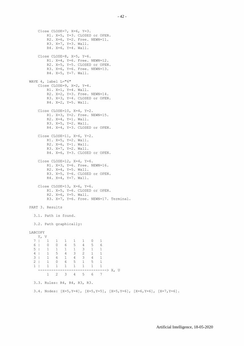
PART 3. Results
3.1. Path is found.
3.2. Path graphically:
LABCOPY
Y, V
7 | 1 1 1 1 1 0 1
6 | 0 0 6 5 4 5 6
5 | 1 1 1 1 3 1 1
4 | 1 5 4 3 2 1 1
3 | 1 6 1 4 3 4 1
2 | 1 0 6 5 1 5 1
1 | 1 1 1 1 1 1 1
-------------------------------> X, U
1 2 3 4 5 6 7
3.3. Rules: R4, R4, R3, R3.
3.4. Nodes: [X=5,Y=4], [X=5,Y=5], [X=5,Y=6], [X=6,Y=6], [X=7,Y=6].
- 43 -
Artificial Intelligence, 18-05-2020
9. Breadth-first search in a graph
The BFS algorithm is presented below according to the book by Earl Hunt (1978), section
10.1.1. The algorithm finds the path with fewest edges. See also
https://en.wikipedia.org/wiki/Breadth-first_search.
INPUT: 1) a graph G; 2) a starting vertex s; 3) a terminal vertex t.
OUTPUT: the shortest path from s to t.
The algorithm operates with two lists, OPEN and CLOSED, which initially are empty.
1. Add the starting vertex s to OPEN.
2. If OPEN is empty then there is no path. Return FAIL. This happens in the case of a
disconnected graph; see Fig. 9.1.
3. Close the first vertex n from OPEN: move it from OPEN to CLOSED. If n is the terminal
vertex, then collect the path and finish.
4. Take the set S(n) of adjacent vertices to n. Add all the vertices from S(n), which are neither
in OPEN nor in CLOSED, to the end of OPEN. Formally,
OPEN := OPEN S(n)/(OPENCLOSED) .
5. Go to 2.
Fig. 9.1. A sample disconnected graph with
no path between s and t
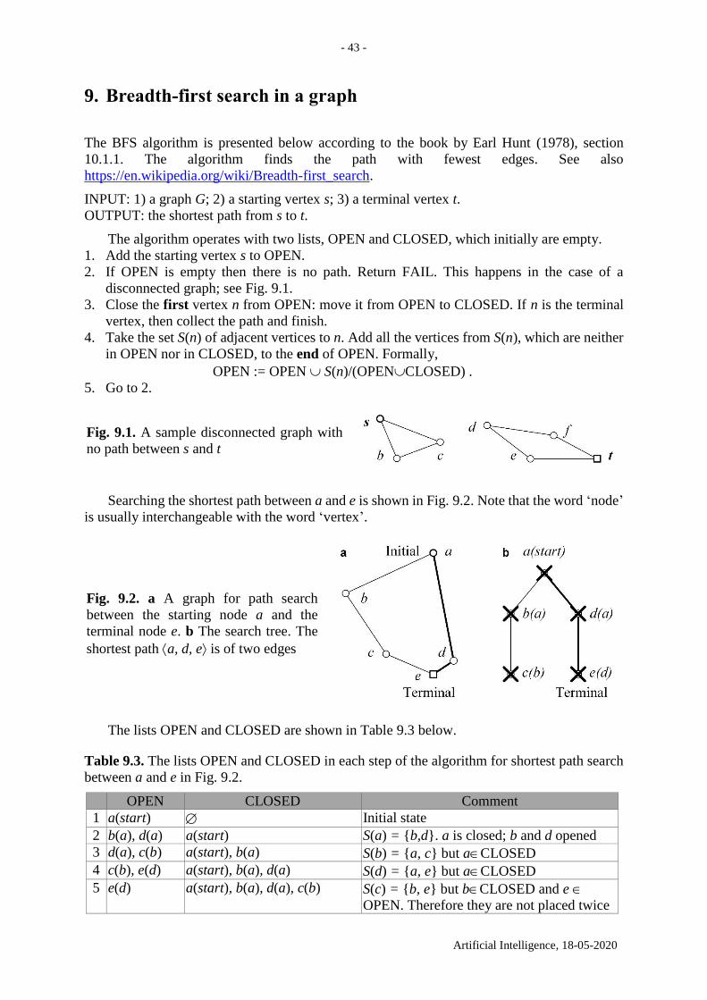
Searching the shortest path between a and e is shown in Fig. 9.2. Note that the word ‘node’
is usually interchangeable with the word ‘vertex’.
Fig. 9.2. a A graph for path search
between the starting node a and the
terminal node e. b The search tree. The
shortest path a, d, e is of two edges
The lists OPEN and CLOSED are shown in Table 9.3 below.
Table 9.3. The lists OPEN and CLOSED in each step of the algorithm for shortest path search
between a and e in Fig. 9.2.
OPEN CLOSED Comment
1 a(start) Initial state
2 b(a), d(a) a(start) S(a) = {b,d}. a is closed; b and d opened
3 d(a), c(b) a(start), b(a) S(b) = {a, c} but aCLOSED
4 c(b), e(d) a(start), b(a), d(a) S(d) = {a, e} but aCLOSED
5 e(d) a(start), b(a), d(a), c(b) S(c) = {b, e} but bCLOSED and e
OPEN. Therefore they are not placed twice
- 44 -
Artificial Intelligence, 18-05-2020
6 a(start), b(a), d(a), c(b), e(d) The terminal node e is being closed. Its
children are not analysed
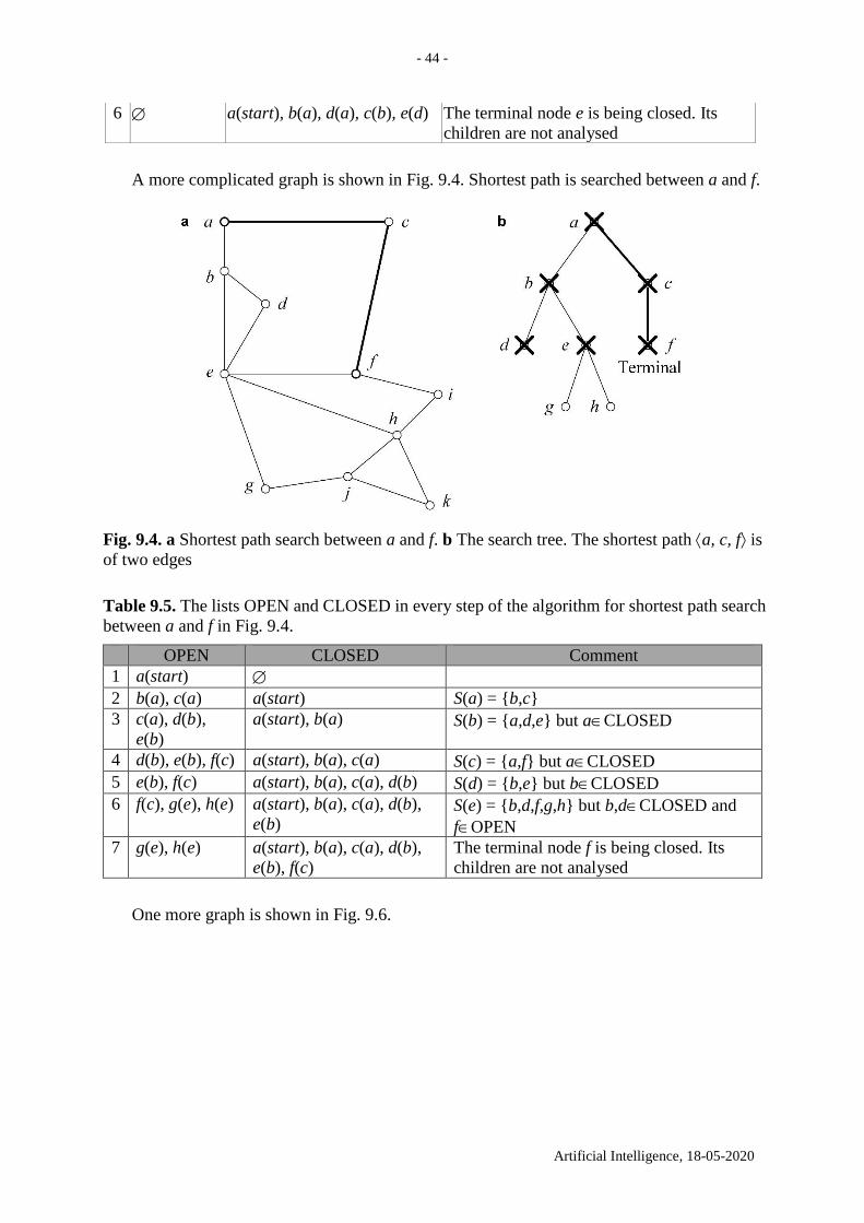
A more complicated graph is shown in Fig. 9.4. Shortest path is searched between a and f.
Fig. 9.4. a Shortest path search between a and f. b The search tree. The shortest path a, c, f is
of two edges
Table 9.5. The lists OPEN and CLOSED in every step of the algorithm for shortest path search
between a and f in Fig. 9.4.
OPEN CLOSED Comment
1 a(start)
2 b(a), c(a) a(start) S(a) = {b,c}
3 c(a), d(b),
e(b)
a(start), b(a) S(b) = {a,d,e} but aCLOSED
4 d(b), e(b), f(c) a(start), b(a), c(a) S(c) = {a,f} but aCLOSED
5 e(b), f(c) a(start), b(a), c(a), d(b) S(d) = {b,e} but bCLOSED
6 f(c), g(e), h(e) a(start), b(a), c(a), d(b),
e(b) S(e) = {b,d,f,g,h} but b,dCLOSED and
fOPEN
7 g(e), h(e) a(start), b(a), c(a), d(b),
e(b), f(c)
The terminal node f is being closed. Its
children are not analysed
One more graph is shown in Fig. 9.6.
- 45 -
Artificial Intelligence, 18-05-2020
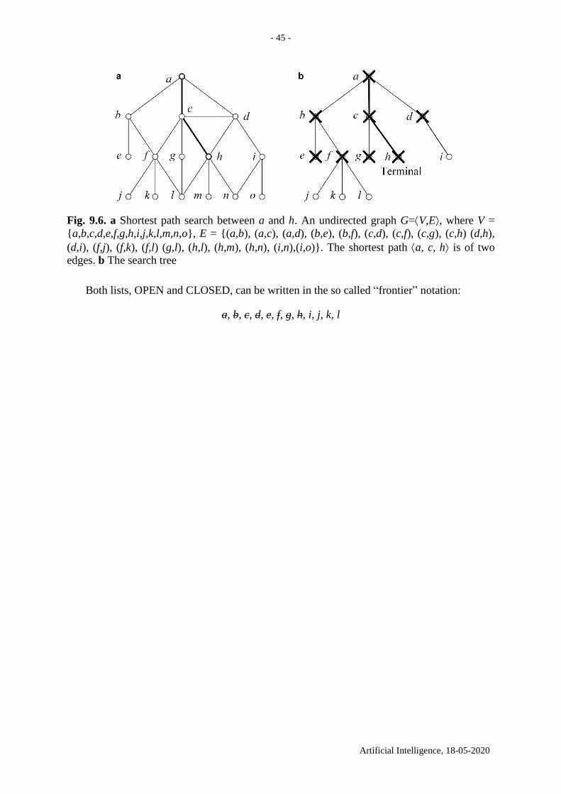
Fig. 9.6. a Shortest path search between a and h. An undirected graph G=V,E, where V =
{a,b,c,d,e,f,g,h,i,j,k,l,m,n,o}, E = {(a,b), (a,c), (a,d), (b,e), (b,f), (c,d), (c,f), (c,g), (c,h) (d,h),
(d,i), (f,j), (f,k), (f,l) (g,l), (h,l), (h,m), (h,n), (i,n),(i,o)}. The shortest path a, c, h is of two
edges. b The search tree
Both lists, OPEN and CLOSED, can be written in the so called “frontier” notation:
a, b, c, d, e, f, g, h, i, j, k, l
- 46 -
Artificial Intelligence, 18-05-2020
10. Shortest path problem in a graph with edge weights
Suppose a graph with nonnegative edge weights. We provide an algorithm to search for the
shortest path from an initial node s to a terminal node t. This is a classic algorithm and is
presented in textbooks, see e.g. (Hunt 1978, 10.1.2). When each edge in the graph has unit
weight 1, this is equivalent to finding the path with fewest edges (see previous section).
This algorithm is a variant of Dijkstra’s algorithm which is conceived by Dutch computer
scientist Edsger Dijkstra in 1956. Dijkstra’s algorithm to find the shortest path between s and t
starts from s, picks the unvisited vertex with the lowest distance, calculates the distance through
it to each unvisited neighbour, and updates the neighbour’s distance if smaller, see
https://en.wikipedia.org/wiki/Dijkstra%27s_algorithm.
INPUT: 1) a graph G with edge weights; 2) a starting node s; 3) a terminal node t.
OUTPUT: the shortest path from s to t.
Initially the lists OPEN and CLOSED are empty.
1. Add the starting node s to OPEN.
2. If OPEN is empty then there is no path. Return FAIL. This happens in the case of a
disconnected graph.
3. Close the first node n from OPEN: move it from OPEN to CLOSED. Here n is the node
with the shortest distance from s. (OPEN is sorted in this way.) If n is the terminal node
then collect the path and return it.
4. Take the set S(n) of nodes, which are adjacent to n. Add to OPEN those nodes, which are
not in CLOSED; formally, OPEN :=OPEN S(n)/CLOSED. For each n* from
S(n)/CLOSED, calculate its distance and assign it in OPEN. Formally,
n* S(n)/CLOSED, assign pathweight(s,n*) := pathweight(s,n) + edgeweight(n,n*). Sort
OPEN. For each n* which appears twice (with the old pathweight and a new one) update
the distance for a smaller one.
5. Go to 2.
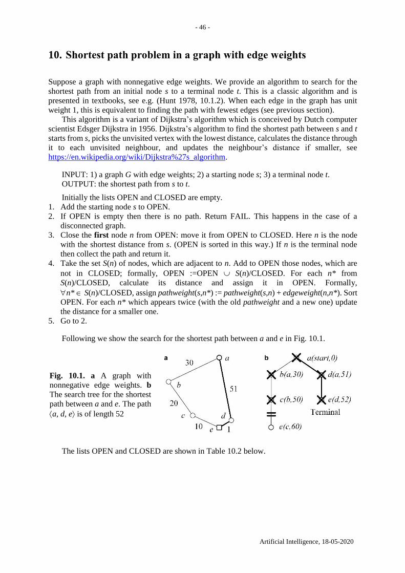
Following we show the search for the shortest path between a and e in Fig. 10.1.
Fig. 10.1. a A graph with
nonnegative edge weights. b
The search tree for the shortest
path between a and e. The path
a, d, e is of length 52
The lists OPEN and CLOSED are shown in Table 10.2 below.
- 47 -
Artificial Intelligence, 18-05-2020
Table 10.2. The lists OPEN and CLOSED in each step of the algorithm for shortest path search
between a and e in Fig. 10.1. The path a(start,0), d(a,51), e(d,52) is of length 52.
OPEN CLOSED Comment
1 a(start,0)
2 b(a,30), d(a,51) a(start,0) S(a) = {b,d }
3 c(b,50), d(a,51) a(start,0), b(a,30) S(b) = {a,c} but aCLOSED
4 d(a,51), e(c,60) a(start,0), b(a,30), c(b,50) S(c) = {b,e} but bCLOSED
5 e(d,52) a(start,0), b(a,30), c(b,50),
d(a,51) S(d) = {a,e} but aCLOSED and
eOPEN. New cost e(d,52) is better
than the old one e(c,60). Take it
6 a(start,0), b(a,30), c(b,50),
d(a,51), e(d,52)
The terminal node e is closed
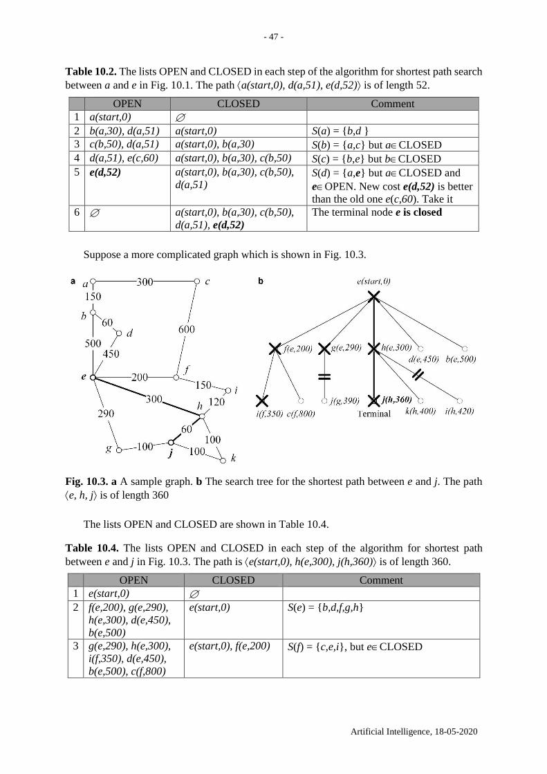
Suppose a more complicated graph which is shown in Fig. 10.3.
Fig. 10.3. a A sample graph. b The search tree for the shortest path between e and j. The path
e, h, j is of length 360
The lists OPEN and CLOSED are shown in Table 10.4.
Table 10.4. The lists OPEN and CLOSED in each step of the algorithm for shortest path
between e and j in Fig. 10.3. The path is e(start,0), h(e,300), j(h,360) is of length 360.
OPEN CLOSED Comment
1 e(start,0)
2 f(e,200), g(e,290),
h(e,300), d(e,450),
b(e,500)
e(start,0) S(e) = {b,d,f,g,h}
3 g(e,290), h(e,300),
i(f,350), d(e,450),
b(e,500), c(f,800)
e(start,0), f(e,200) S(f) = {c,e,i}, but eCLOSED

- 48 -
Artificial Intelligence, 18-05-2020
4 h(e,300), i(f,350),
j(g,390), d(e,450),
b(e,500), c(f,800)
e(start,0), f(e,200),
g(e,290) S(g) = {e,j}, but eCLOSED
5 i(f,350), j(h,360),
k(h,400), d(e,450),
b(e,500), c(f,800)
e(start,0), f(e,200),
g(e,290), h(e,300) S(h) = {e,i,j,k}, but eCLOSED and
i,jOPEN. New cost i(h,420) is worse
than the old i(f,350); therefore the old one
is taken. New cost j(h,360) is better than
the old j(g,390); therefore the new one is
taken
6 j(h,360), k(h,400),
d(e,450), b(e,500),
c(f,800)
e(start,0), f(e,200),
g(e,290), h(e,300),
i(f,350)
S(i) = {f,h}, but f,hCLOSED
7 k(h,400), d(e,450),
b(e,500), c(f,800)
e(start,0), f(e,200),
g(e,290), h(e,300),
i(f,350), j(h,360)
The terminal node j is closed. Its children
are not analysed
- 49 -
Artificial Intelligence, 18-05-2020
11. Depth-first search in a graph with no weights. The solver and
the planner
Suppose an agent knows the graph. Does it make sense for the agent to use depth-first search
to find a path between two nodes? Yes, suppose the agent walks in the graph like in a park,
does not need the shortest path and is satisfied with any long path.
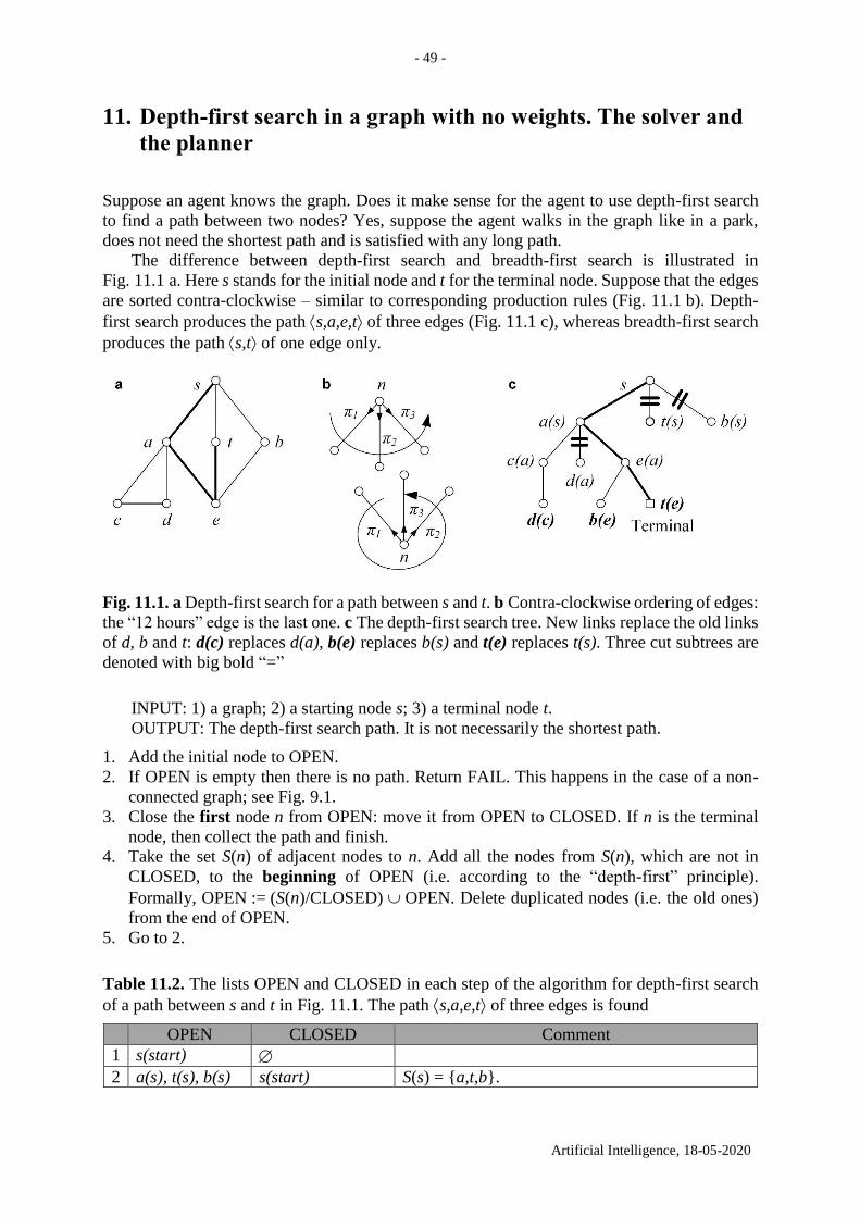
The difference between depth-first search and breadth-first search is illustrated in
Fig. 11.1 a. Here s stands for the initial node and t for the terminal node. Suppose that the edges
are sorted contra-clockwise – similar to corresponding production rules (Fig. 11.1 b). Depth-
first search produces the path s,a,e,t of three edges (Fig. 11.1 c), whereas breadth-first search
produces the path s,t of one edge only.
Fig. 11.1. a Depth-first search for a path between s and t. b Contra-clockwise ordering of edges:
the “12 hours” edge is the last one. c The depth-first search tree. New links replace the old links
of d, b and t: d(c) replaces d(a), b(e) replaces b(s) and t(e) replaces t(s). Three cut subtrees are
denoted with big bold “=”
INPUT: 1) a graph; 2) a starting node s; 3) a terminal node t.
OUTPUT: The depth-first search path. It is not necessarily the shortest path.
1. Add the initial node to OPEN.
2. If OPEN is empty then there is no path. Return FAIL. This happens in the case of a non-
connected graph; see Fig. 9.1.
3. Close the first node n from OPEN: move it from OPEN to CLOSED. If n is the terminal
node, then collect the path and finish.
4. Take the set S(n) of adjacent nodes to n. Add all the nodes from S(n), which are not in
CLOSED, to the beginning of OPEN (i.e. according to the “depth-first” principle).
Formally, OPEN := (S(n)/CLOSED) OPEN. Delete duplicated nodes (i.e. the old ones)
from the end of OPEN.
5. Go to 2.
Table 11.2. The lists OPEN and CLOSED in each step of the algorithm for depth-first search
of a path between s and t in Fig. 11.1. The path s,a,e,t of three edges is found
OPEN CLOSED Comment
1 s(start)
2 a(s), t(s), b(s) s(start) S(s) = {a,t,b}.

- 50 -
Artificial Intelligence, 18-05-2020
3 c(a), d(a), e(a),
t(s), b(s)
s(start), a(s) S(a) = {c,d,e,s}. But sCLOSED.
4 d(c), e(a), t(s),
b(s)
s(start), a(s), c(a) S(c) = {d,a}. But aCLOSED and dOPEN.
Therefore d(c), which is opened later, is placed
into the OPEN’s head and d(a) is deleted the
from OPEN’s tail.
5 e(a), t(s), b(s) s(start), a(s), c(a),
d(c) S(d) = {c,a}. But c,aCLOSED
6 b(e), t(e) s(start), a(s), c(a),
d(c), e(a) S(e) = {a,b,t}. But aCLOSED and b,tOPEN.
Therefore b(e) and t(e), which are opened later,
are placed into the OPEN’s head and t(s) and b(s)
are deleted the from OPEN’s tail.
7 t(e) s(start), a(s), c(a),
d(c), e(a), b(e) S(b) = {s,e}. But s,eCLOSED.
8 s(start), a(s), c(a),
d(c), e(a), b(e),
t(e)
The terminal node t is closed. The resulting path
is collected backwards: t is reached from e, e
from a, and a from s.
The solver and the planner. The depth-first search strategy is usually used by solvers and
the breadth-first search by planners. Solver is shorthand for problem-solver and a solving agent.
Planner – a planning agent. Their differences:
Solver Planner
1 Does not have a map Has a map
2 Does not find the shortest path Can find the shortest path
3 Depth-first search Normally breadth-first search
4 Onetime usage of the path Multiple usage of the path
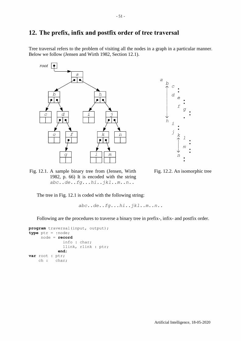
- 51 -
Artificial Intelligence, 18-05-2020
12. The prefix, infix and postfix order of tree traversal
Tree traversal refers to the problem of visiting all the nodes in a graph in a particular manner.
Below we follow (Jensen and Wirth 1982, Section 12.1).
Fig. 12.1. A sample binary tree from (Jensen, Wirth
1982, p. 66) It is encoded with the string abc..de..fg...hi..jkl..m..n..
Fig. 12.2. An isomorphic tree
The tree in Fig. 12.1 is coded with the following string:
abc..de..fg...hi..jkl..m..n..
Following are the procedures to traverse a binary tree in prefix-, infix- and postfix order.
program traversal(input, output);
type ptr = ↑node;
node = record
info : char;
llink, rlink : ptr;
end;
var root : ptr;
ch : char;
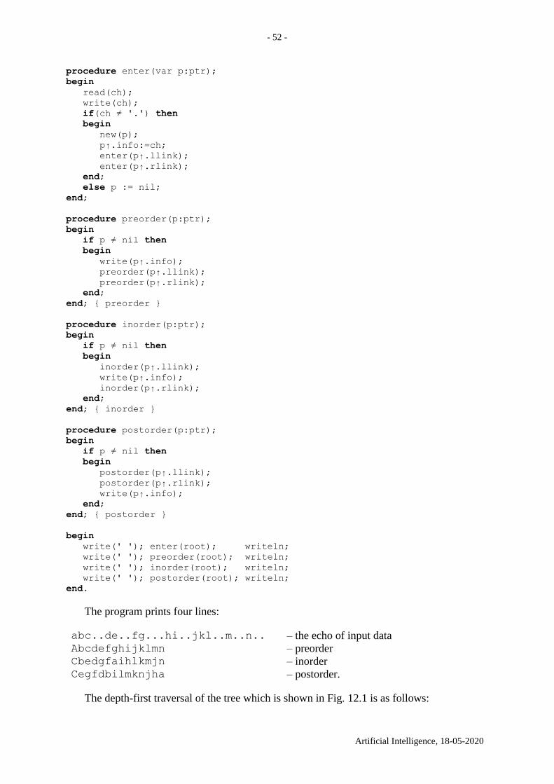
- 52 -
Artificial Intelligence, 18-05-2020
procedure enter(var p:ptr);
begin
read(ch);
write(ch);
if(ch ≠ '.') then
begin
new(p);
p↑.info:=ch;
enter(p↑.llink);
enter(p↑.rlink);
end;
else p := nil;
end;
procedure preorder(p:ptr);
begin
if p ≠ nil then
begin
write(p↑.info);
preorder(p↑.llink);
preorder(p↑.rlink);
end;
end; { preorder }
procedure inorder(p:ptr);
begin
if p ≠ nil then
begin
inorder(p↑.llink);
write(p↑.info);
inorder(p↑.rlink);
end;
end; { inorder }
procedure postorder(p:ptr);
begin
if p ≠ nil then
begin
postorder(p↑.llink);
postorder(p↑.rlink);
write(p↑.info);
end;
end; { postorder }
begin
write(' '); enter(root); writeln;
write(' '); preorder(root); writeln;
write(' '); inorder(root); writeln;
write(' '); postorder(root); writeln;
end.
The program prints four lines:
abc..de..fg...hi..jkl..m..n.. – the echo of input data Abcdefghijklmn – preorder Cbedgfaihlkmjn – inorder Cegfdbilmknjha – postorder.
The depth-first traversal of the tree which is shown in Fig. 12.1 is as follows:
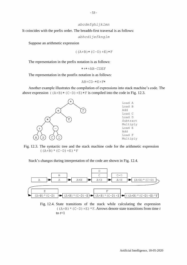
- 53 -
Artificial Intelligence, 18-05-2020
abcdefghijklmn
It coincides with the prefix order. The breadth-first traversal is as follows:
abhcdijefknglm
Suppose an arithmetic expression
((A+B)(C–D)+E)F
The representation in the prefix notation is as follows:
++AB–CDEF
The representation in the postfix notation is as follows:
AB+CD–E+F
Another example illustrates the compilation of expressions into stack machine’s code. The
above expression ((A+B)(C–D)+E)F is compiled into the code in Fig. 12.3.
Load A
Load B
Add
Load C
Load D
Subtract
Multiply
Load E
Add
Load F
Multiply
Fig. 12.3. The syntactic tree and the stack machine code for the arithmetic expression ((A+B)*(C–D)+E)*F
Stack’s changes during interpretation of the code are shown in Fig. 12.4.
Fig. 12.4. State transitions of the stack while calculating the expression
((A+B)*(C–D)+E)*F. Arrows denote state transitions from time t
to t+1
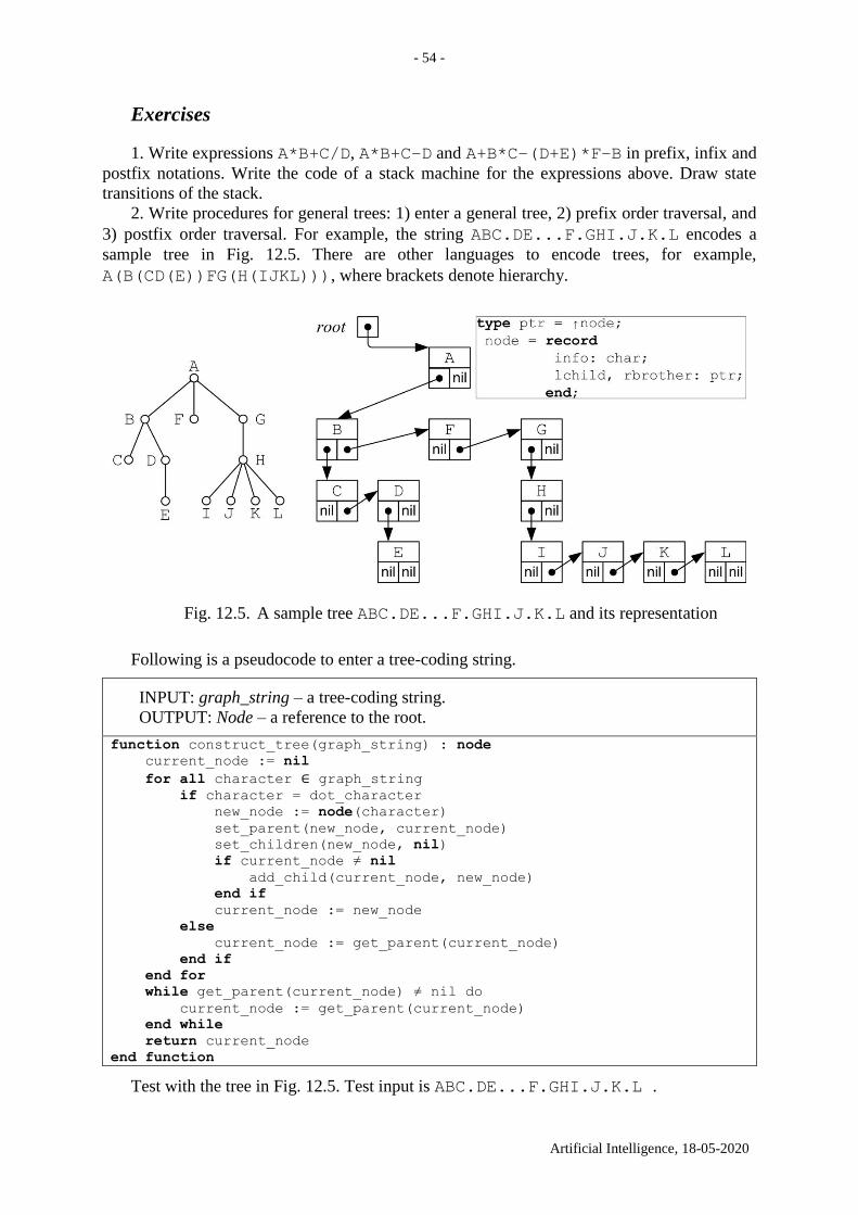
- 54 -
Artificial Intelligence, 18-05-2020
Exercises
1. Write expressions A*B+C/D, A*B+C–D and A+B*C–(D+E)*F–B in prefix, infix and
postfix notations. Write the code of a stack machine for the expressions above. Draw state
transitions of the stack.
2. Write procedures for general trees: 1) enter a general tree, 2) prefix order traversal, and
3) postfix order traversal. For example, the string ABC.DE...F.GHI.J.K.L encodes a
sample tree in Fig. 12.5. There are other languages to encode trees, for example,
A(B(CD(E))FG(H(IJKL))), where brackets denote hierarchy.
Fig. 12.5. A sample tree ABC.DE...F.GHI.J.K.L and its representation
Following is a pseudocode to enter a tree-coding string.
INPUT: graph_string – a tree-coding string.
OUTPUT: Node – a reference to the root.
function construct_tree(graph_string) : node
current_node := nil
for all character ∈ graph_string if character = dot_character
new_node := node(character)
set_parent(new_node, current_node)
set_children(new_node, nil)
if current_node ≠ nil
add_child(current_node, new_node)
end if
current_node := new_node
else
current_node := get_parent(current_node)
end if
end for
while get_parent(current_node) ≠ nil do
current_node := get_parent(current_node)
end while
return current_node
end function
Test with the tree in Fig. 12.5. Test input is ABC.DE...F.GHI.J.K.L .
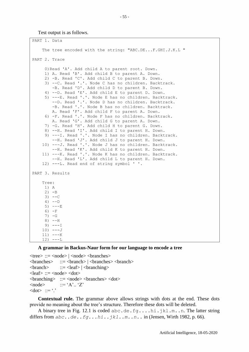
- 55 -
Artificial Intelligence, 18-05-2020
Test output is as follows.
PART 1. Data
The tree encoded with the string: "ABC.DE...F.GHI.J.K.L "
PART 2. Trace
0)Read 'A'. Add child A to parent root. Down.
1) A. Read 'B'. Add child B to parent A. Down.
2) -B. Read 'C'. Add child C to parent B. Down.
3) --C. Read '.'. Node C has no children. Backtrack.
-B. Read 'D'. Add child D to parent B. Down.
4) --D. Read 'E'. Add child E to parent D. Down.
5) ---E. Read '.'. Node E has no children. Backtrack.
--D. Read '.'. Node D has no children. Backtrack.
-B. Read '.'. Node B has no children. Backtrack.
A. Read 'F'. Add child F to parent A. Down.
6) -F. Read '.'. Node F has no children. Backtrack.
A. Read 'G'. Add child G to parent A. Down.
7) -G. Read 'H'. Add child H to parent G. Down.
8) --H. Read 'I'. Add child I to parent H. Down.
9) ---I. Read '.'. Node I has no children. Backtrack.
--H. Read 'J'. Add child J to parent H. Down.
10) ---J. Read '.'. Node J has no children. Backtrack.
--H. Read 'K'. Add child K to parent H. Down.
11) ---K. Read '.'. Node K has no children. Backtrack.
--H. Read 'L'. Add child L to parent H. Down.
12) ---L. Read end of string symbol ' '.
PART 3. Results
Tree:
1) A
2) -B
3) --C
4) --D
5) ---E
6) -F
7) -G
8) --H
9) ---I
10) ---J
11) ---K
12) ---L
A grammar in Backus-Naur form for our language to encode a tree
<tree> ::= <node> | <node> <branches>
<branches> ::= <branch> | <branches> <branch>
<branch> ::= <leaf> | <branching>
<leaf> ::= <node> <dot>
<branching> ::= <node> <branches> <dot>
<node> ::= ‘A’.. ‘Z’
<dot> ::= ‘.’
Contextual rule. The grammar above allows strings with dots at the end. These dots
provide no meaning about the tree’s structure. Therefore these dots will be deleted.
A binary tree in Fig. 12.1 is coded abc.de.fg....hi.jkl.m..n. The latter string
differs from abc..de..fg...hi..jkl..m..n.. in (Jensen, Wirth 1982, p. 66).
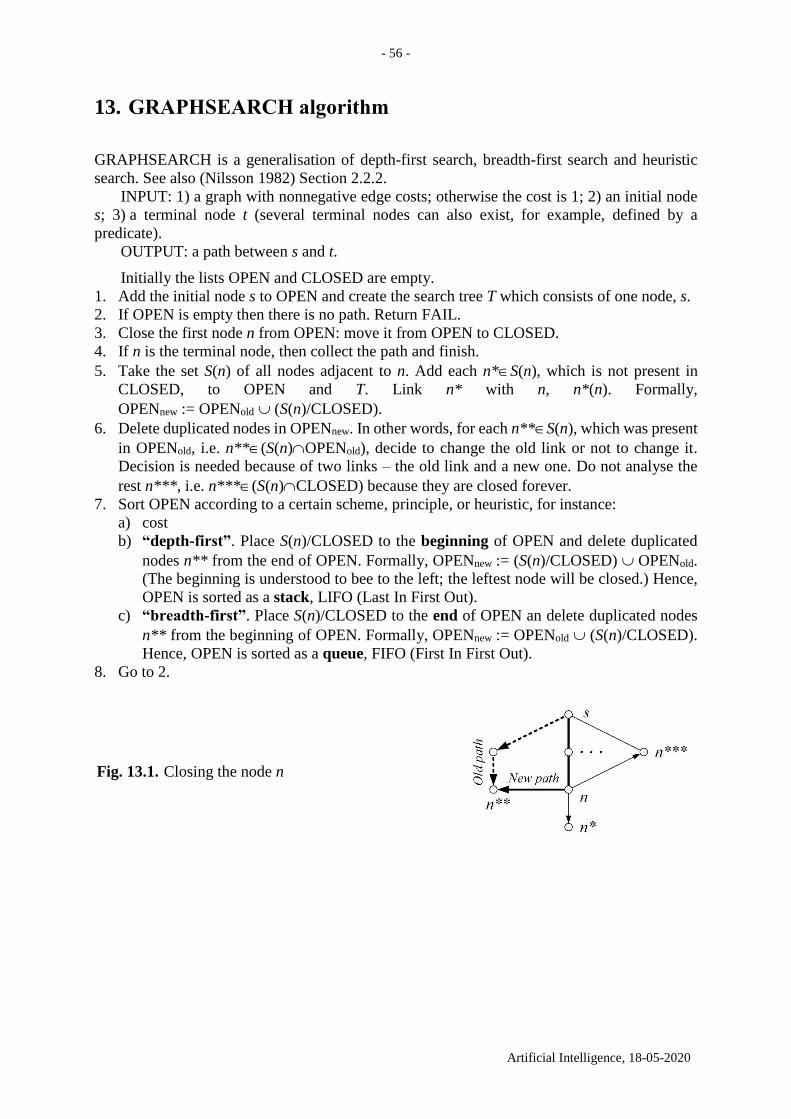
- 56 -
Artificial Intelligence, 18-05-2020
13. GRAPHSEARCH algorithm
GRAPHSEARCH is a generalisation of depth-first search, breadth-first search and heuristic
search. See also (Nilsson 1982) Section 2.2.2.
INPUT: 1) a graph with nonnegative edge costs; otherwise the cost is 1; 2) an initial node
s; 3) a terminal node t (several terminal nodes can also exist, for example, defined by a
predicate).
OUTPUT: a path between s and t.
Initially the lists OPEN and CLOSED are empty.
1. Add the initial node s to OPEN and create the search tree T which consists of one node, s.
2. If OPEN is empty then there is no path. Return FAIL.
3. Close the first node n from OPEN: move it from OPEN to CLOSED.
4. If n is the terminal node, then collect the path and finish.
5. Take the set S(n) of all nodes adjacent to n. Add each n*S(n), which is not present in
CLOSED, to OPEN and T. Link n* with n, n*(n). Formally,
OPENnew := OPENold (S(n)/CLOSED).
6. Delete duplicated nodes in OPENnew. In other words, for each n**S(n), which was present
in OPENold, i.e. n**(S(n)OPENold), decide to change the old link or not to change it.
Decision is needed because of two links – the old link and a new one. Do not analyse the
rest n***, i.e. n***(S(n)CLOSED) because they are closed forever.
7. Sort OPEN according to a certain scheme, principle, or heuristic, for instance:
a) cost
b) “depth-first”. Place S(n)/CLOSED to the beginning of OPEN and delete duplicated
nodes n** from the end of OPEN. Formally, OPENnew := (S(n)/CLOSED) OPENold.
(The beginning is understood to bee to the left; the leftest node will be closed.) Hence,
OPEN is sorted as a stack, LIFO (Last In First Out).
c) “breadth-first”. Place S(n)/CLOSED to the end of OPEN an delete duplicated nodes
n** from the beginning of OPEN. Formally, OPENnew := OPENold (S(n)/CLOSED).
Hence, OPEN is sorted as a queue, FIFO (First In First Out).
8. Go to 2.
Fig. 13.1. Closing the node n
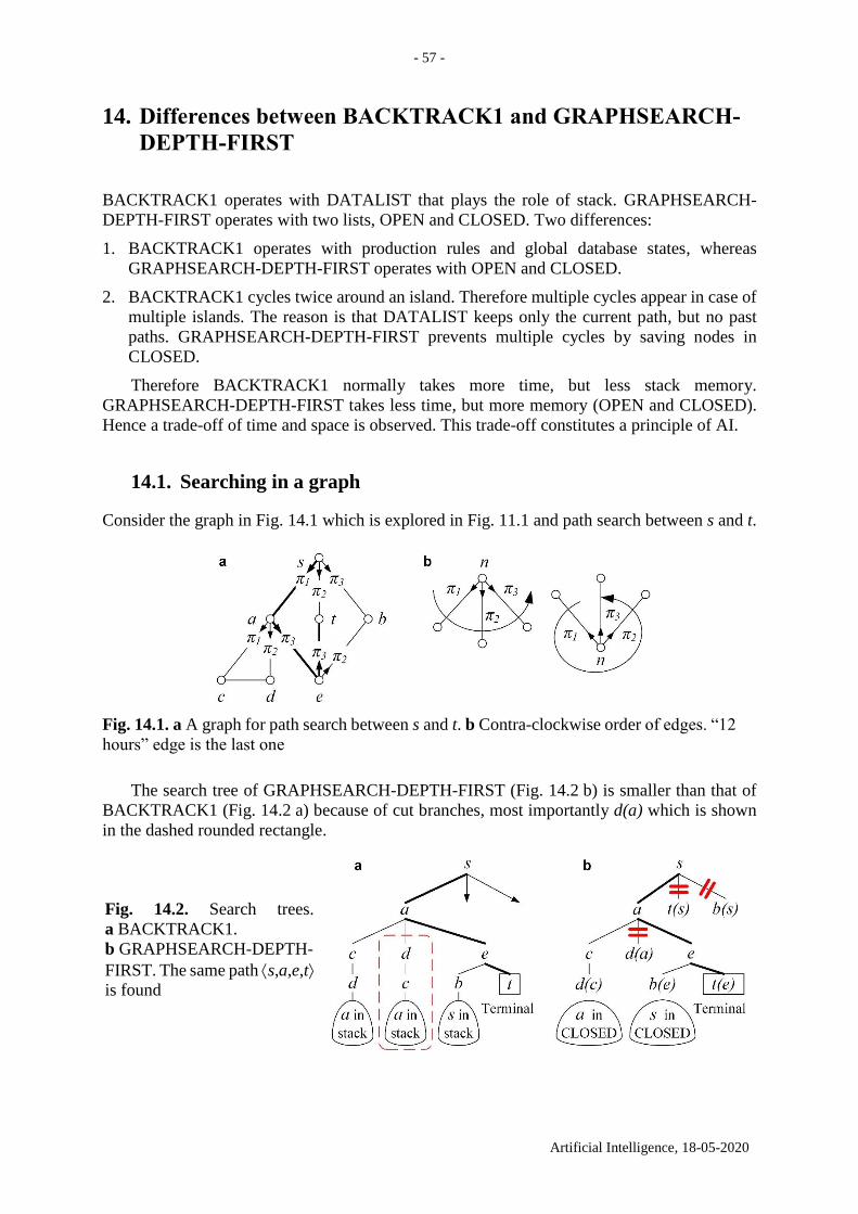
- 57 -
Artificial Intelligence, 18-05-2020
14. Differences between BACKTRACK1 and GRAPHSEARCH-
DEPTH-FIRST
BACKTRACK1 operates with DATALIST that plays the role of stack. GRAPHSEARCH-
DEPTH-FIRST operates with two lists, OPEN and CLOSED. Two differences:
1. BACKTRACK1 operates with production rules and global database states, whereas
GRAPHSEARCH-DEPTH-FIRST operates with OPEN and CLOSED.
2. BACKTRACK1 cycles twice around an island. Therefore multiple cycles appear in case of
multiple islands. The reason is that DATALIST keeps only the current path, but no past
paths. GRAPHSEARCH-DEPTH-FIRST prevents multiple cycles by saving nodes in
CLOSED.
Therefore BACKTRACK1 normally takes more time, but less stack memory.
GRAPHSEARCH-DEPTH-FIRST takes less time, but more memory (OPEN and CLOSED).
Hence a trade-off of time and space is observed. This trade-off constitutes a principle of AI.
14.1. Searching in a graph
Consider the graph in Fig. 14.1 which is explored in Fig. 11.1 and path search between s and t.
Fig. 14.1. a A graph for path search between s and t. b Contra-clockwise order of edges. “12
hours” edge is the last one
The search tree of GRAPHSEARCH-DEPTH-FIRST (Fig. 14.2 b) is smaller than that of
BACKTRACK1 (Fig. 14.2 a) because of cut branches, most importantly d(a) which is shown
in the dashed rounded rectangle.
Fig. 14.2. Search trees.
a BACKTRACK1.
b GRAPHSEARCH-DEPTH-
FIRST. The same path s,a,e,t
is found
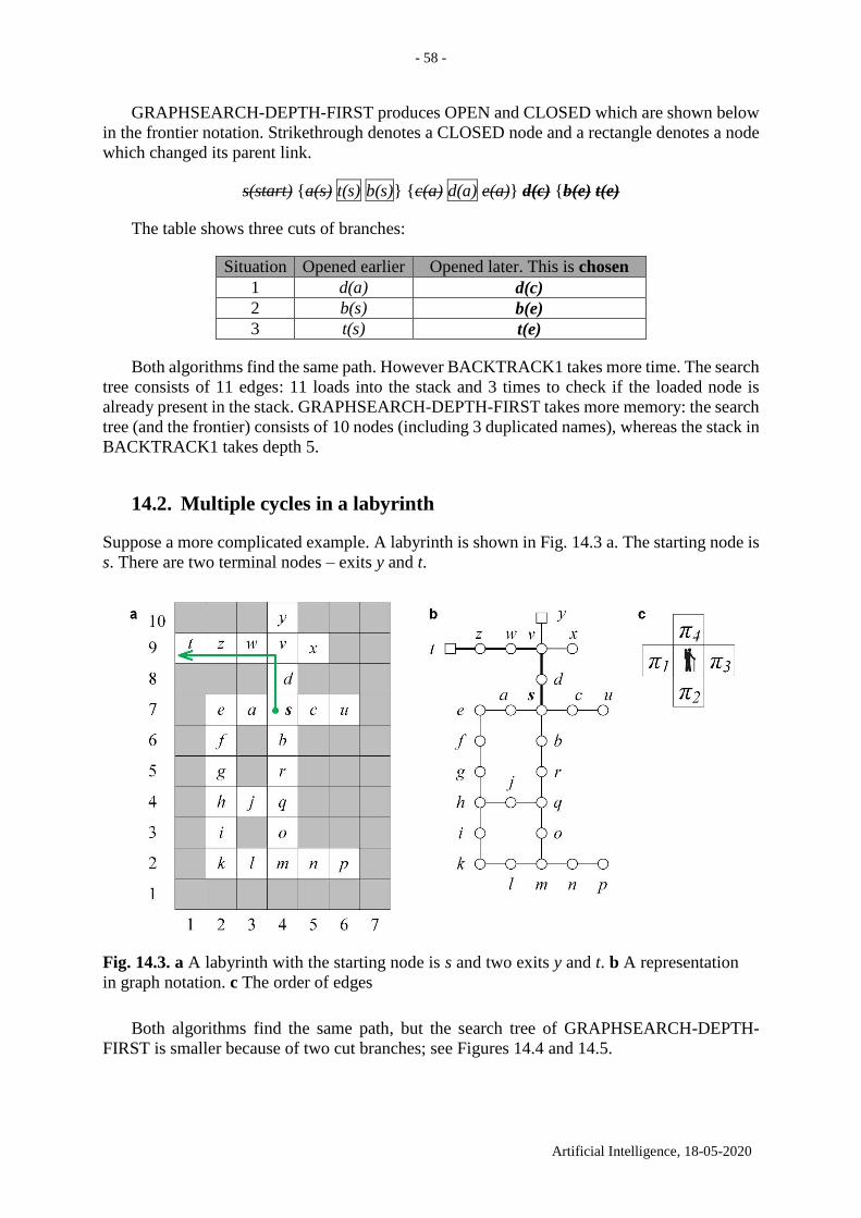
- 58 -
Artificial Intelligence, 18-05-2020
GRAPHSEARCH-DEPTH-FIRST produces OPEN and CLOSED which are shown below
in the frontier notation. Strikethrough denotes a CLOSED node and a rectangle denotes a node
which changed its parent link.
s(start) {a(s) t(s) b(s)} {c(a) d(a) e(a)} d(c) {b(e) t(e)
The table shows three cuts of branches:
Situation Opened earlier Opened later. This is chosen
1 d(a) d(c)
2 b(s) b(e)
3 t(s) t(e)
Both algorithms find the same path. However BACKTRACK1 takes more time. The search
tree consists of 11 edges: 11 loads into the stack and 3 times to check if the loaded node is
already present in the stack. GRAPHSEARCH-DEPTH-FIRST takes more memory: the search
tree (and the frontier) consists of 10 nodes (including 3 duplicated names), whereas the stack in
BACKTRACK1 takes depth 5.
14.2. Multiple cycles in a labyrinth
Suppose a more complicated example. A labyrinth is shown in Fig. 14.3 a. The starting node is
s. There are two terminal nodes – exits y and t.
Fig. 14.3. a A labyrinth with the starting node is s and two exits y and t. b A representation
in graph notation. c The order of edges
Both algorithms find the same path, but the search tree of GRAPHSEARCH-DEPTH-
FIRST is smaller because of two cut branches; see Figures 14.4 and 14.5.
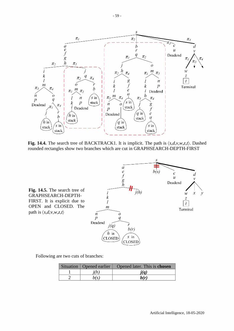
- 59 -
Artificial Intelligence, 18-05-2020
Fig. 14.4. The search tree of BACKTRACK1. It is implicit. The path is s,d,v,w,z,t. Dashed
rounded rectangles show two branches which are cut in GRAPHSEARCH-DEPTH-FIRST
Fig. 14.5. The search tree of
GRAPHSEARCH-DEPTH-
FIRST. It is explicit due to
OPEN and CLOSED. The
path is s,d,v,w,z,t
Following are two cuts of branches:
Situation Opened earlier Opened later. This is chosen
1 j(h) j(q)
2 b(s) b(r)
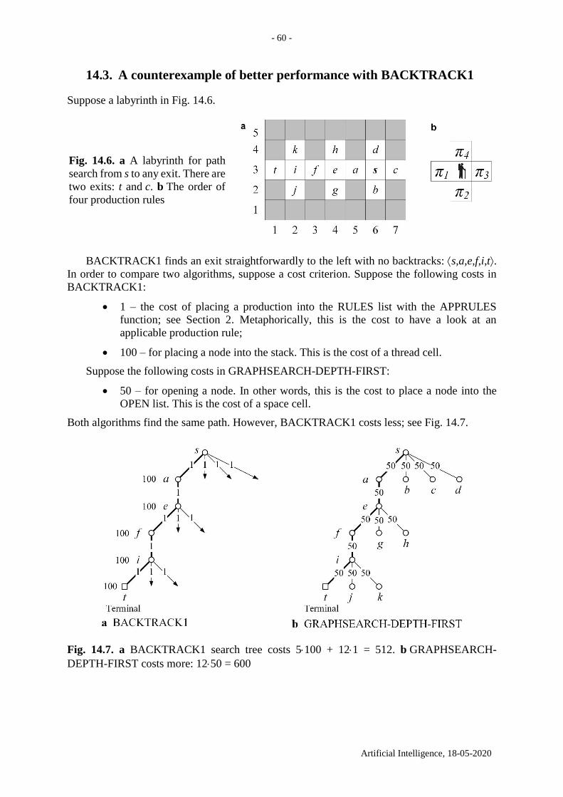
- 60 -
Artificial Intelligence, 18-05-2020
14.3. A counterexample of better performance with BACKTRACK1
Suppose a labyrinth in Fig. 14.6.
Fig. 14.6. a A labyrinth for path
search from s to any exit. There are
two exits: t and c. b The order of
four production rules
BACKTRACK1 finds an exit straightforwardly to the left with no backtracks: s,a,e,f,i,t.
In order to compare two algorithms, suppose a cost criterion. Suppose the following costs in
BACKTRACK1:
1 – the cost of placing a production into the RULES list with the APPRULES
function; see Section 2. Metaphorically, this is the cost to have a look at an
applicable production rule;
100 – for placing a node into the stack. This is the cost of a thread cell.
Suppose the following costs in GRAPHSEARCH-DEPTH-FIRST:
50 – for opening a node. In other words, this is the cost to place a node into the
OPEN list. This is the cost of a space cell.
Both algorithms find the same path. However, BACKTRACK1 costs less; see Fig. 14.7.
Fig. 14.7. a BACKTRACK1 search tree costs 5100 + 121 = 512. b GRAPHSEARCH-
DEPTH-FIRST costs more: 1250 = 600

- 61 -
Artificial Intelligence, 18-05-2020
Exerxise
Which algorithm – GRAPHSEARCH-DEPTH-
FIRST or BACKTRACK1 – performs better
according to time and space in this labyrinth?
The starting node is s. Draw the search tree with
the costs: lookup – 1, thread – 100, and one
memory cell in OPEN – 50.
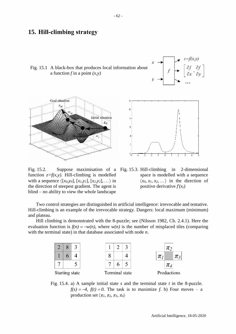
- 62 -
Artificial Intelligence, 18-05-2020
15. Hill-climbing strategy
Fig. 15.1 A black-box that produces local information about
a function f in a point (x,y)
Fig. 15.2. Suppose maximisation of a
function z=f(x,y). Hill-climbing is modelled
with a sequence [x0,y0], [x1,y1], [x2,y2], in
the direction of steepest gradient. The agent is
blind – no ability to view the whole landscape
Fig. 15.3. Hill-climbing in 2-dimensional
space is modelled with a sequence
x0, x1, x2, in the direction of
positive derivative f'(xi)
Two control strategies are distinguished in artificial intelligence: irrevocable and tentative.
Hill-climbing is an example of the irrevocable strategy. Dangers: local maximum (minimum)
and plateau.
Hill climbing is demonstrated with the 8-puzzle; see (Nilsson 1982, Ch. 2.4.1). Here the
evaluation function is f(n) w(n), where w(n) is the number of misplaced tiles (comparing
with the terminal state) in that database associated with node n.
Fig. 15.4. a) A sample initial state s and the terminal state t in the 8-puzzle.
f(s) 4, f(t) 0. The task is to maximize f. b) Four moves – a
production set π1, π2, π3, π4
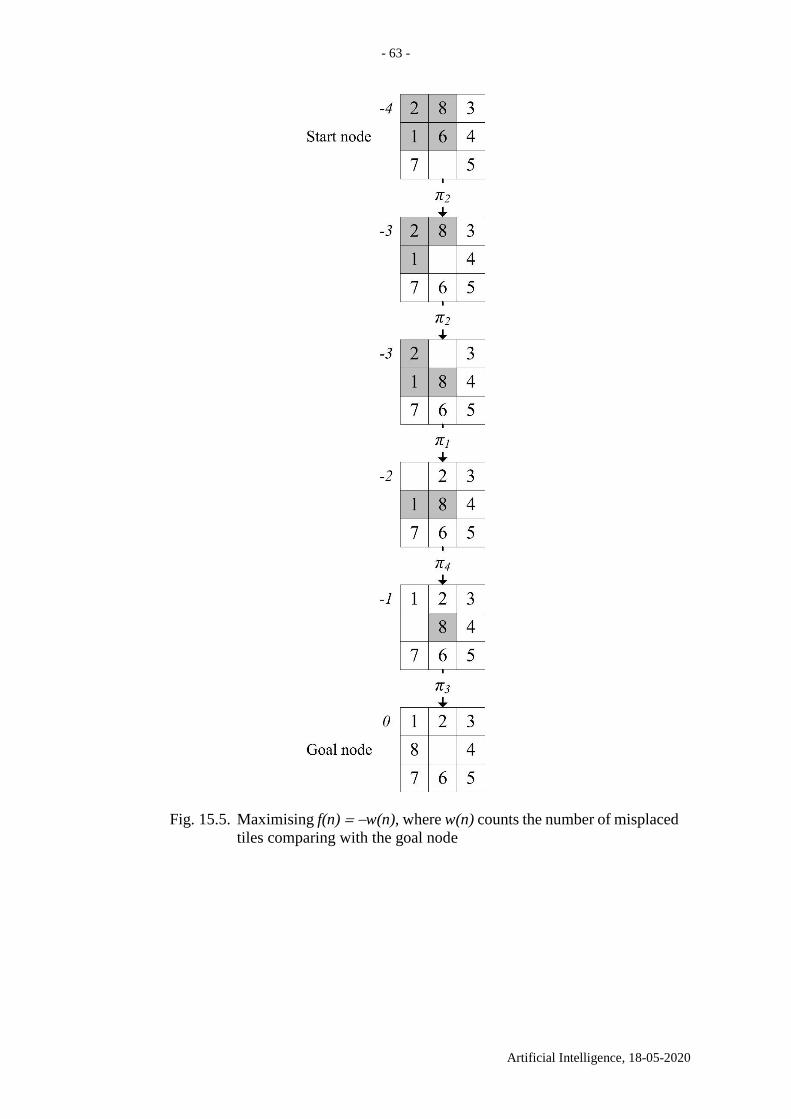
- 63 -
Artificial Intelligence, 18-05-2020
Fig. 15.5. Maximising f(n) w(n), where w(n) counts the number of misplaced
tiles comparing with the goal node
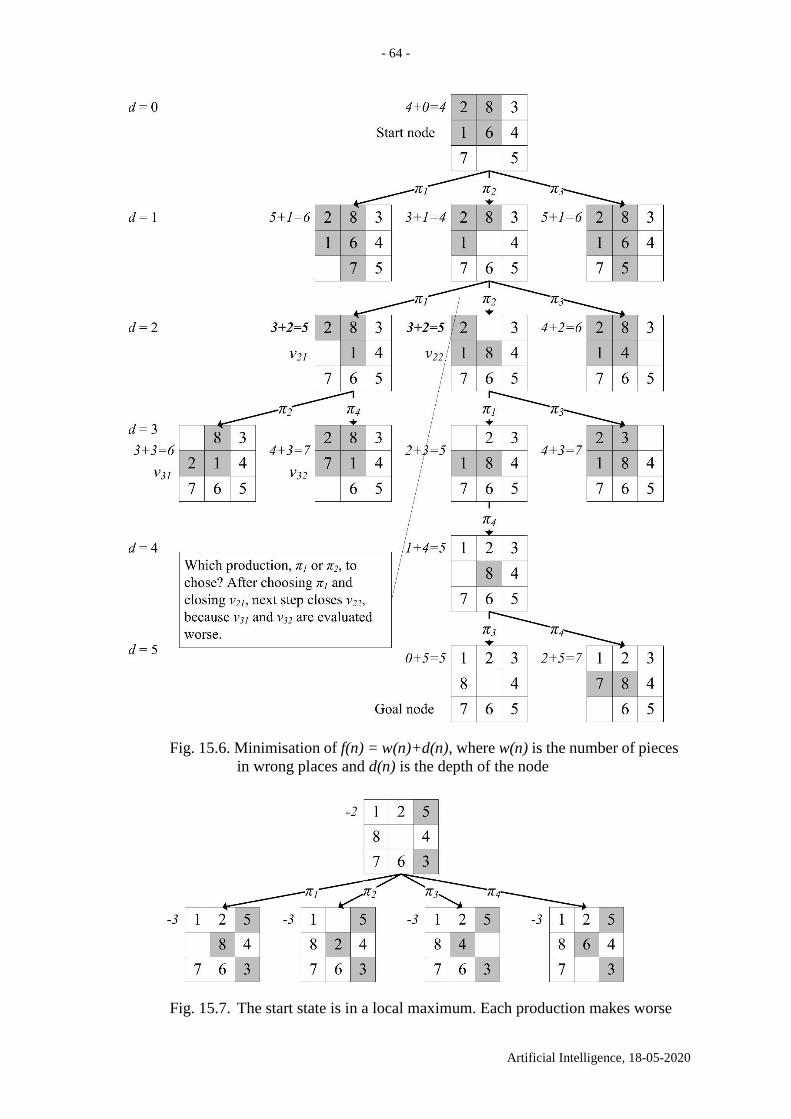
- 64 -
Artificial Intelligence, 18-05-2020
Fig. 15.6. Minimisation of f(n) = w(n)+d(n), where w(n) is the number of pieces
in wrong places and d(n) is the depth of the node
Fig. 15.7. The start state is in a local maximum. Each production makes worse
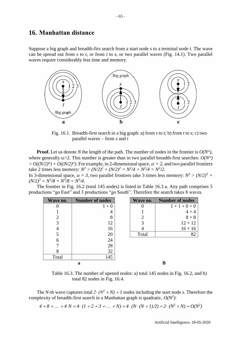
- 65 -
Artificial Intelligence, 18-05-2020
16. Manhattan distance
Suppose a big graph and breadth-firs search from a start node s to a terminal node t. The wave
can be spread out from s to t, or from t to s, or two parallel waves (Fig. 14.1). Two parallel
waves require considerably less time and memory.
Fig. 16.1. Breadth-first search in a big graph: a) from s to t; b) from t to s; c) two
parallel waves – from s and t
Proof. Let us denote N the length of the path. The number of nodes in the frontier is O(N),
where generally >2. This number is greater than in two parallel breadth-first searches: O(N)
> O((N/2)) + O((N/2)). For example, in 2-dimensional space, = 2, and two parallel frontiers
take 2 times less memory: N2 > (N/2)2 + (N/2)2 = N2/4 + N2/4 = N2/2.
In 3-dimensional space, = 3, two parallel frontiers take 3 times less memory: N3 > (N/2)3 +
(N/2)3 = N3/8 + N3/8 = N3/4.
The frontier in Fig. 16.2 (total 145 nodes) is listed in Table 16.3 a. Any path comprises 5
productions “go East” and 3 productions “go South”. Therefore the search takes 8 waves.
Wave no. Number of nodes Wave no. Number of nodes
0 1 + 0 0 1 + 1 + 0 + 0
1 4 1 4 + 4
2 8 2 8 + 8
3 12 3 12 + 12
4 16 4 16 + 16
5 20 Total 82
6 24
7 28
8 32
Total 145
a B
Table 16.3. The number of opened nodes: a) total 145 nodes in Fig. 16.2, and b)
total 82 nodes in Fig. 16.4.
The N-th wave captures total 2· (N2 N) 1 nodes including the start node s. Therefore the
complexity of breadth-first search in a Manhattan graph is quadratic, O(N2):
4 8 4·N 4· (1 2 3 N) 4· (N· (N 1)2) 2· (N2 N) O(N2)
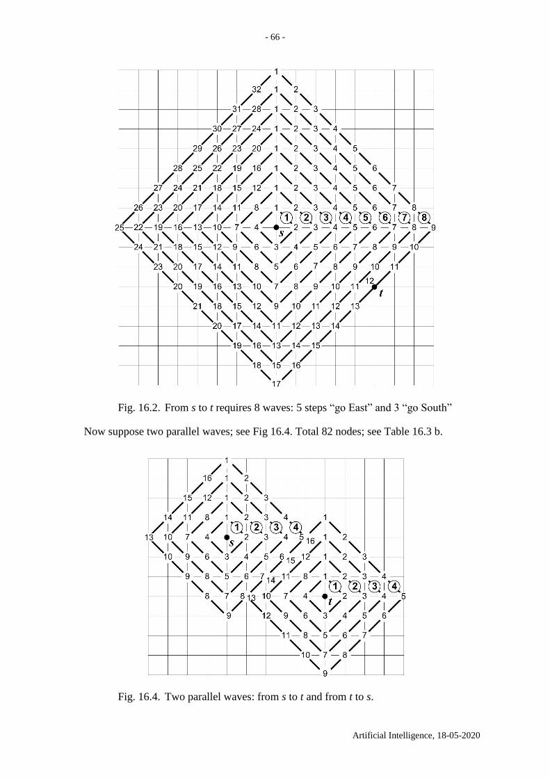
- 66 -
Artificial Intelligence, 18-05-2020
Fig. 16.2. From s to t requires 8 waves: 5 steps “go East” and 3 “go South”
Now suppose two parallel waves; see Fig 16.4. Total 82 nodes; see Table 16.3 b.
Fig. 16.4. Two parallel waves: from s to t and from t to s.
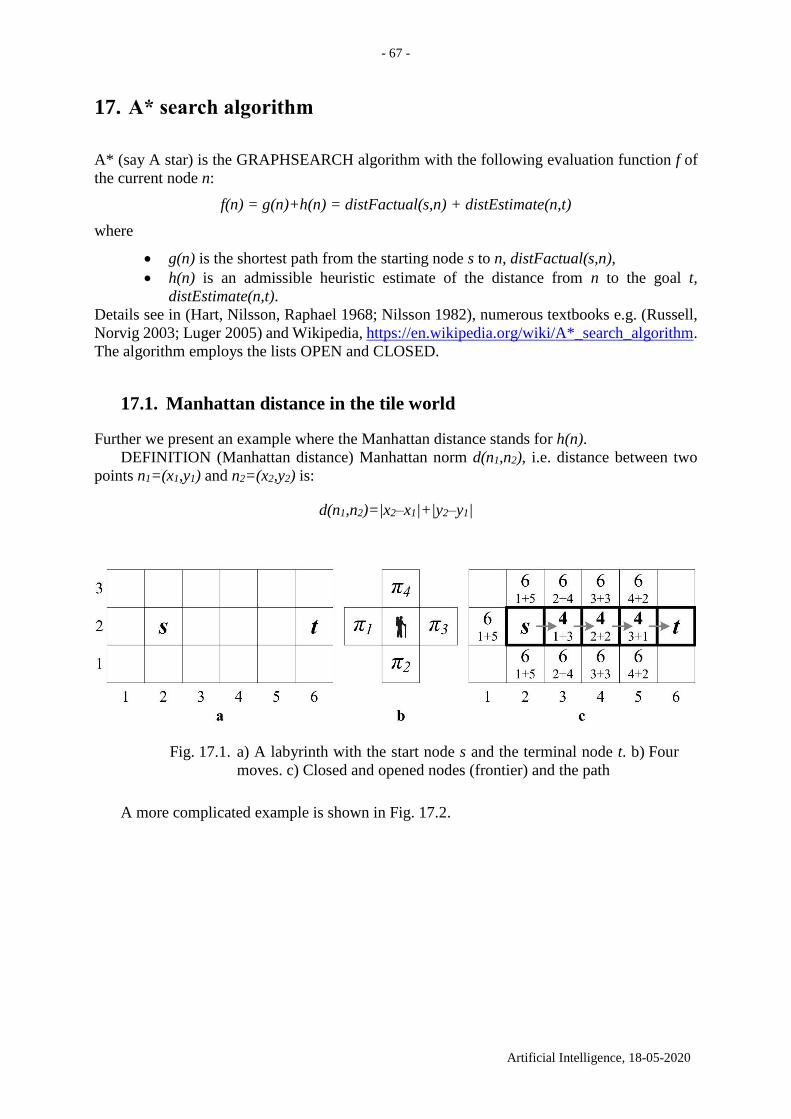
- 67 -
Artificial Intelligence, 18-05-2020
17. A* search algorithm
A* (say A star) is the GRAPHSEARCH algorithm with the following evaluation function f of
the current node n:
f(n) = g(n)+h(n) = distFactual(s,n) + distEstimate(n,t)
where
g(n) is the shortest path from the starting node s to n, distFactual(s,n),
h(n) is an admissible heuristic estimate of the distance from n to the goal t,
distEstimate(n,t).
Details see in (Hart, Nilsson, Raphael 1968; Nilsson 1982), numerous textbooks e.g. (Russell,
Norvig 2003; Luger 2005) and Wikipedia, https://en.wikipedia.org/wiki/A*_search_algorithm.
The algorithm employs the lists OPEN and CLOSED.
17.1. Manhattan distance in the tile world
Further we present an example where the Manhattan distance stands for h(n).
DEFINITION (Manhattan distance) Manhattan norm d(n1,n2), i.e. distance between two
points n1=(x1,y1) and n2=(x2,y2) is:
d(n1,n2)=|x2–x1|+|y2–y1|
Fig. 17.1. a) A labyrinth with the start node s and the terminal node t. b) Four
moves. c) Closed and opened nodes (frontier) and the path
A more complicated example is shown in Fig. 17.2.
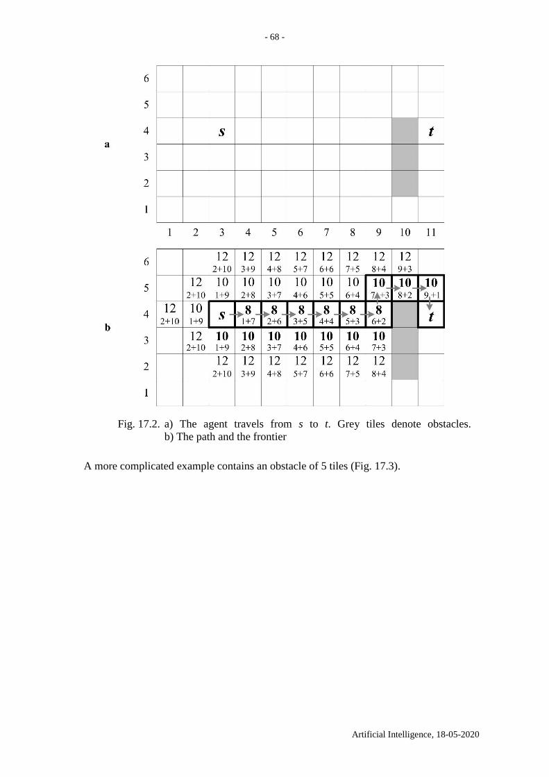
- 68 -
Artificial Intelligence, 18-05-2020
Fig. 17.2. a) The agent travels from s to t. Grey tiles denote obstacles.
b) The path and the frontier
A more complicated example contains an obstacle of 5 tiles (Fig. 17.3).
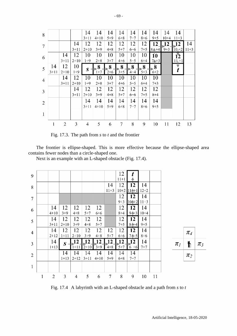
- 69 -
Artificial Intelligence, 18-05-2020
Fig. 17.3. The path from s to t and the frontier
The frontier is ellipse-shaped. This is more effective because the ellipse-shaped area
contains fewer nodes than a circle-shaped one.
Next is an example with an L-shaped obstacle (Fig. 17.4).
Fig. 17.4 A labyrinth with an L-shaped obstacle and a path from s to t
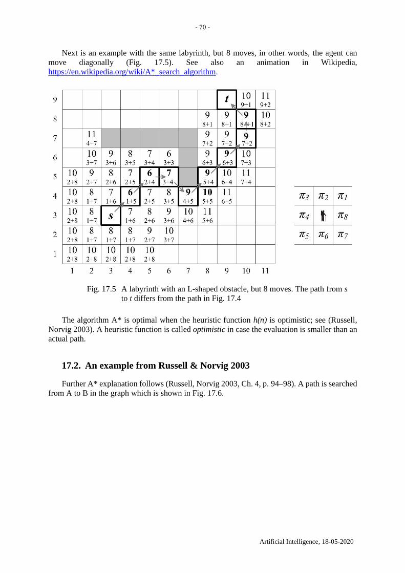
- 70 -
Artificial Intelligence, 18-05-2020
Next is an example with the same labyrinth, but 8 moves, in other words, the agent can
move diagonally (Fig. 17.5). See also an animation in Wikipedia,
https://en.wikipedia.org/wiki/A*_search_algorithm.
Fig. 17.5 A labyrinth with an L-shaped obstacle, but 8 moves. The path from s
to t differs from the path in Fig. 17.4
The algorithm A* is optimal when the heuristic function h(n) is optimistic; see (Russell,
Norvig 2003). A heuristic function is called optimistic in case the evaluation is smaller than an
actual path.
17.2. An example from Russell & Norvig 2003
Further A* explanation follows (Russell, Norvig 2003, Ch. 4, p. 94–98). A path is searched
from A to B in the graph which is shown in Fig. 17.6.
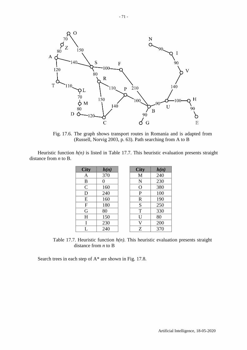
- 71 -
Artificial Intelligence, 18-05-2020
Fig. 17.6. The graph shows transport routes in Romania and is adapted from
(Russell, Norvig 2003, p. 63). Path searching from A to B
Heuristic function h(n) is listed in Table 17.7. This heuristic evaluation presents straight
distance from n to B.
City h(n) City h(n)
A 370 M 240
B 0 N 230
C 160 O 380
D 240 P 100
E 160 R 190
F 180 S 250
G 80 T 330
H 150 U 80
I 230 V 200
L 240 Z 370
Table 17.7. Heuristic function h(n). This heuristic evaluation presents straight
distance from n to B
Search trees in each step of A* are shown in Fig. 17.8.
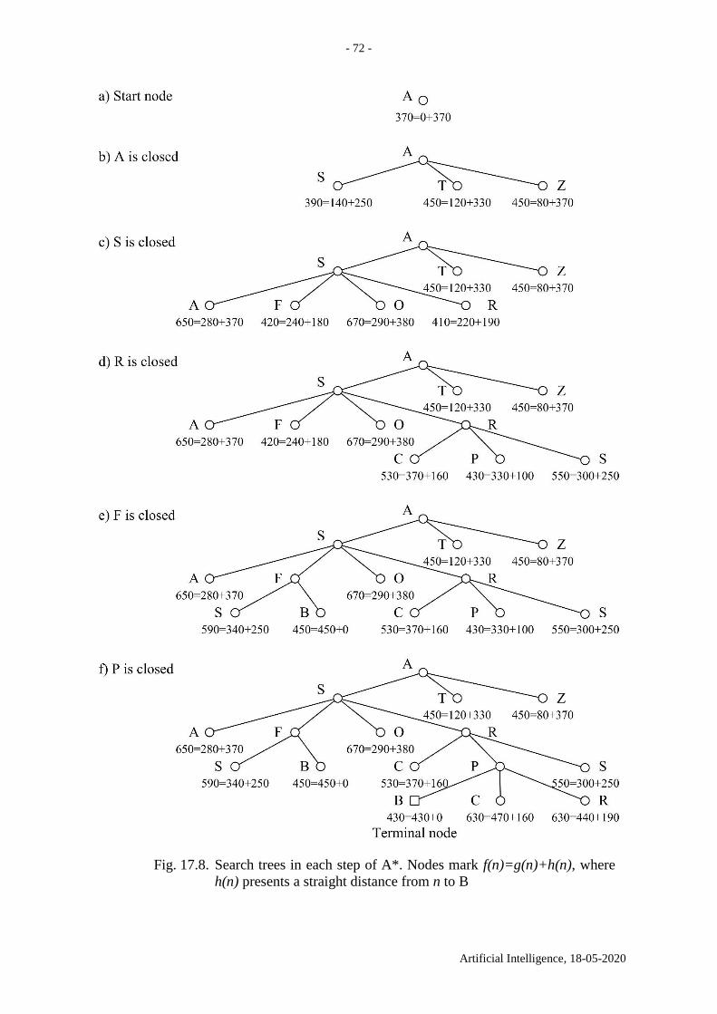
- 72 -
Artificial Intelligence, 18-05-2020
Fig. 17.8. Search trees in each step of A*. Nodes mark f(n)=g(n)+h(n), where
h(n) presents a straight distance from n to B
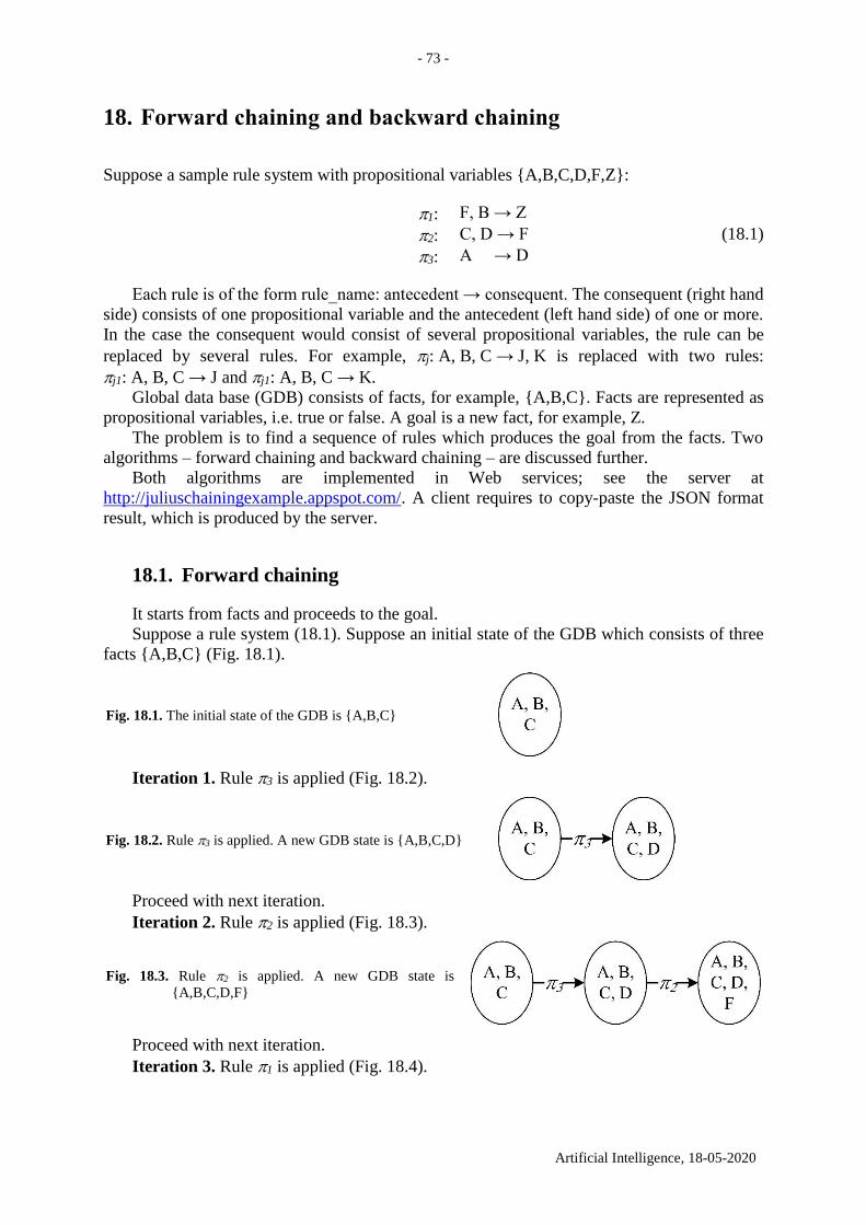
- 73 -
Artificial Intelligence, 18-05-2020
18. Forward chaining and backward chaining
Suppose a sample rule system with propositional variables {A,B,C,D,F,Z}:
1: F, B → Z
2: C, D → F (18.1)
3: A → D
Each rule is of the form rule_name: antecedent → consequent. The consequent (right hand
side) consists of one propositional variable and the antecedent (left hand side) of one or more.
In the case the consequent would consist of several propositional variables, the rule can be
replaced by several rules. For example, j: A, B, C → J, K is replaced with two rules:
j1: A, B, C → J and j1: A, B, C → K.
Global data base (GDB) consists of facts, for example, {A,B,C}. Facts are represented as
propositional variables, i.e. true or false. A goal is a new fact, for example, Z.
The problem is to find a sequence of rules which produces the goal from the facts. Two
algorithms – forward chaining and backward chaining – are discussed further.
Both algorithms are implemented in Web services; see the server at
http://juliuschainingexample.appspot.com/. A client requires to copy-paste the JSON format
result, which is produced by the server.
18.1. Forward chaining
It starts from facts and proceeds to the goal.
Suppose a rule system (18.1). Suppose an initial state of the GDB which consists of three
facts {A,B,C} (Fig. 18.1).
Fig. 18.1. The initial state of the GDB is {A,B,C}
Iteration 1. Rule 3 is applied (Fig. 18.2).
Fig. 18.2. Rule 3 is applied. A new GDB state is {A,B,C,D}
Proceed with next iteration.
Iteration 2. Rule 2 is applied (Fig. 18.3).
Fig. 18.3. Rule 2 is applied. A new GDB state is
{A,B,C,D,F}
Proceed with next iteration.
Iteration 3. Rule 1 is applied (Fig. 18.4).
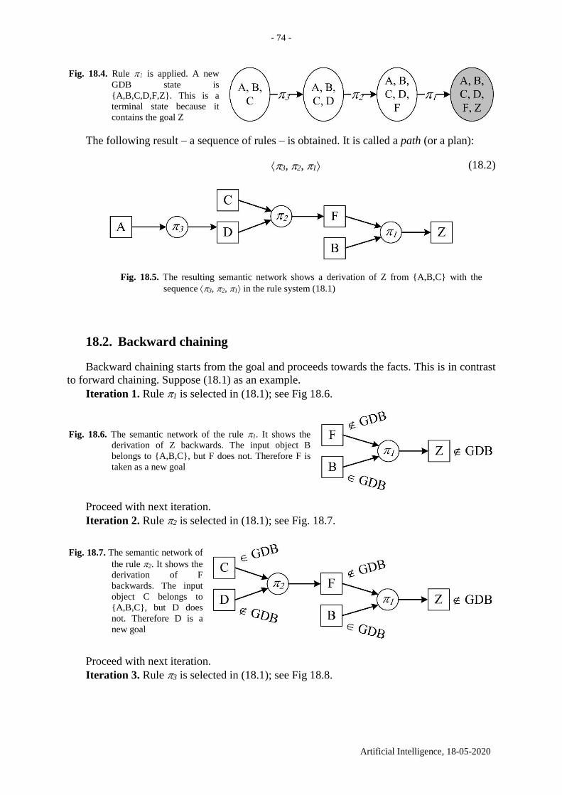
- 74 -
Artificial Intelligence, 18-05-2020
Fig. 18.4. Rule 1 is applied. A new
GDB state is
{A,B,C,D,F,Z}. This is a
terminal state because it
contains the goal Z
The following result – a sequence of rules – is obtained. It is called a path (or a plan):
3, 2, 1 (18.2)
Fig. 18.5. The resulting semantic network shows a derivation of Z from {A,B,C} with the
sequence 3, 2, 1 in the rule system (18.1)
18.2. Backward chaining
Backward chaining starts from the goal and proceeds towards the facts. This is in contrast
to forward chaining. Suppose (18.1) as an example.
Iteration 1. Rule 1 is selected in (18.1); see Fig 18.6.
Fig. 18.6. The semantic network of the rule 1. It shows the
derivation of Z backwards. The input object B
belongs to {A,B,C}, but F does not. Therefore F is
taken as a new goal
Proceed with next iteration.
Iteration 2. Rule 2 is selected in (18.1); see Fig. 18.7.
Fig. 18.7. The semantic network of
the rule 2. It shows the
derivation of F
backwards. The input
object C belongs to
{A,B,C}, but D does
not. Therefore D is a
new goal
Proceed with next iteration.
Iteration 3. Rule 3 is selected in (18.1); see Fig 18.8.
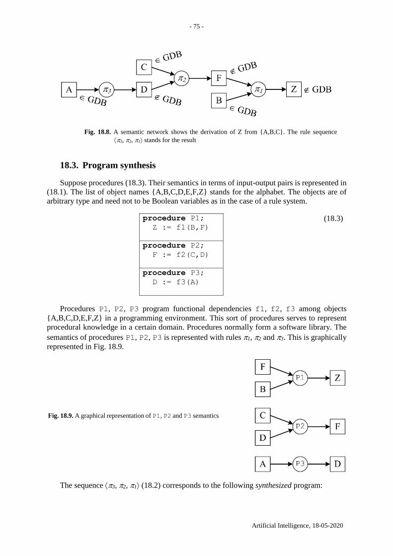
- 75 -
Artificial Intelligence, 18-05-2020
Fig. 18.8. A semantic network shows the derivation of Z from {A,B,C}. The rule sequence
3, 2, 1 stands for the result
18.3. Program synthesis
Suppose procedures (18.3). Their semantics in terms of input-output pairs is represented in
(18.1). The list of object names {A,B,C,D,E,F,Z} stands for the alphabet. The objects are of
arbitrary type and need not to be Boolean variables as in the case of a rule system.
procedure P1;
Z := f1(B,F)
(18.3)
procedure P2;
F := f2(C,D)
procedure P3;
D := f3(A)
Procedures P1, P2, P3 program functional dependencies f1, f2, f3 among objects
{A,B,C,D,E,F,Z} in a programming environment. This sort of procedures serves to represent
procedural knowledge in a certain domain. Procedures normally form a software library. The
semantics of procedures P1, P2, P3 is represented with rules 1, 2 and 3. This is graphically
represented in Fig. 18.9.
Fig. 18.9. A graphical representation of P1, P2 and P3 semantics
The sequence 3, 2, 1 (18.2) corresponds to the following synthesized program:
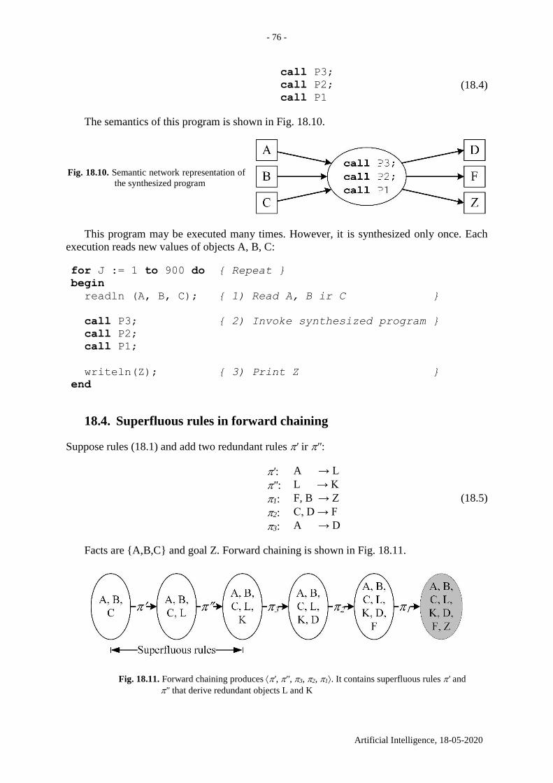
- 76 -
Artificial Intelligence, 18-05-2020
call P3;
call P2; (18.4) call P1
The semantics of this program is shown in Fig. 18.10.
Fig. 18.10. Semantic network representation of
the synthesized program
This program may be executed many times. However, it is synthesized only once. Each
execution reads new values of objects A, B, C:
for J := 1 to 900 do { Repeat }
begin
readln (A, B, C); { 1) Read A, B ir C }
call P3; { 2) Invoke synthesized program }
call P2;
call P1;
writeln(Z); { 3) Print Z }
end
18.4. Superfluous rules in forward chaining
Suppose rules (18.1) and add two redundant rules ' ir ":
': A → L
": L → K
1: F, B → Z (18.5)
2: C, D → F
3: A → D
Facts are {A,B,C} and goal Z. Forward chaining is shown in Fig. 18.11.
Fig. 18.11. Forward chaining produces ', ", 3, 2, 1. It contains superfluous rules ' and
" that derive redundant objects L and K
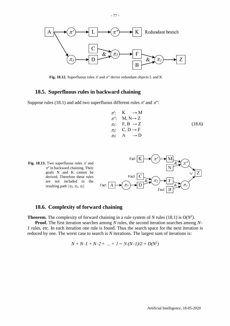
- 77 -
Artificial Intelligence, 18-05-2020
Fig. 18.12. Superfluous rules ' and " derive redundant objects L and K
18.5. Superfluous rules in backward chaining
Suppose rules (18.1) and add two superfluous different rules ' and ":
': K → M
": M, N→ Z
1: F, B → Z (18.6)
2: C, D → F
3: A → D
Fig. 18.13. Two superfluous rules ' and
" in backward chaining. Their
goals N and K cannot be
derived. Therefore these rules
are not included in the
resulting path 3, 2, 1
18.6. Complexity of forward chaining
Theorem. The complexity of forward chaining in a rule system of N rules (18.1) is O(N2).
Proof. The first iteration searches among N rules, the second iteration searches among N–
1 rules, etc. In each iteration one rule is found. Thus the search space for the next iteration is
reduced by one. The worst case to search is N iterations. The largest sum of iterations is:
N + N–1 + N–2 + … + 1 = N(N–1)/2 = O(N2)
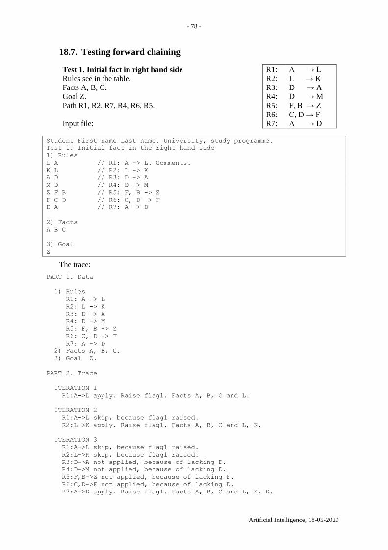
- 78 -
Artificial Intelligence, 18-05-2020
18.7. Testing forward chaining
Test 1. Initial fact in right hand side R1: A → L
Rules see in the table.
Facts A, B, C.
Goal Z.
Path R1, R2, R7, R4, R6, R5.
Input file:
R2: L → K
R3: D → A
R4: D → M
R5: F, B → Z
R6: C, D → F
R7: A → D
Student First name Last name. University, study programme.
Test 1. Initial fact in the right hand side
1) Rules
L A // R1: A -> L. Comments.
K L // R2: L -> K
A D // R3: D -> A
M D // R4: D -> M
Z F B // R5: F, B -> Z
F C D // R6: C, D -> F
D A // R7: A -> D
2) Facts
A B C
3) Goal
Z
The trace:
PART 1. Data
1) Rules
R1: A -> L
R2: L -> K
R3: D -> A
R4: D -> M
R5: F, B -> Z
R6: C, D -> F
R7: A -> D
2) Facts A, B, C.
3) Goal Z.
PART 2. Trace
ITERATION 1
R1:A->L apply. Raise flag1. Facts A, B, C and L.
ITERATION 2
R1:A->L skip, because flag1 raised.
R2:L->K apply. Raise flag1. Facts A, B, C and L, K.
ITERATION 3
R1:A->L skip, because flag1 raised.
R2:L->K skip, because flag1 raised.
R3:D->A not applied, because of lacking D.
R4:D->M not applied, because of lacking D.
R5:F,B->Z not applied, because of lacking F.
R6:C,D->F not applied, because of lacking D.
R7:A->D apply. Raise flag1. Facts A, B, C and L, K, D.
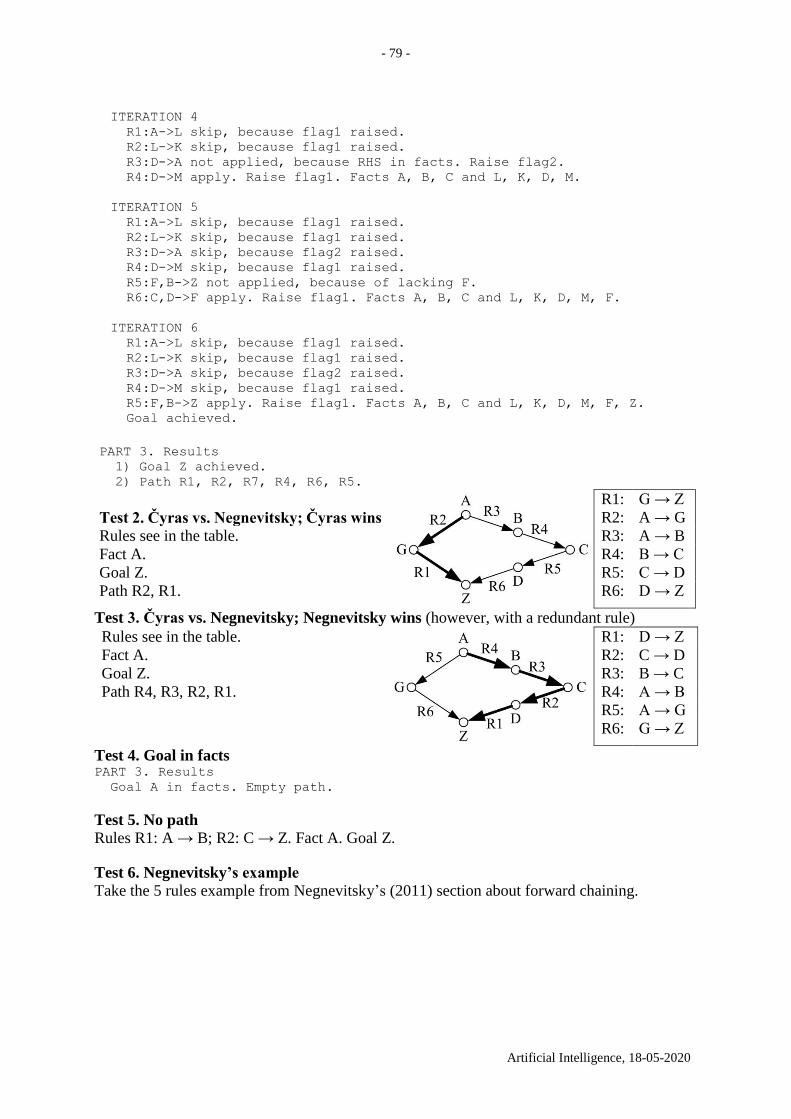
- 79 -
Artificial Intelligence, 18-05-2020
ITERATION 4
R1:A->L skip, because flag1 raised.
R2:L->K skip, because flag1 raised.
R3:D->A not applied, because RHS in facts. Raise flag2.
R4:D->M apply. Raise flag1. Facts A, B, C and L, K, D, M.
ITERATION 5
R1:A->L skip, because flag1 raised.
R2:L->K skip, because flag1 raised.
R3:D->A skip, because flag2 raised.
R4:D->M skip, because flag1 raised.
R5:F,B->Z not applied, because of lacking F.
R6:C,D->F apply. Raise flag1. Facts A, B, C and L, K, D, M, F.
ITERATION 6
R1:A->L skip, because flag1 raised.
R2:L->K skip, because flag1 raised.
R3:D->A skip, because flag2 raised.
R4:D->M skip, because flag1 raised.
R5:F,B->Z apply. Raise flag1. Facts A, B, C and L, K, D, M, F, Z.
Goal achieved.
PART 3. Results
1) Goal Z achieved.
2) Path R1, R2, R7, R4, R6, R5.
R1: G → Z
Test 2. Čyras vs. Negnevitsky; Čyras wins R2: A → G
Rules see in the table. R3: A → B
Fact A. R4: B → C
Goal Z. R5: C → D
Path R2, R1. R6: D → Z
Test 3. Čyras vs. Negnevitsky; Negnevitsky wins (however, with a redundant rule)
Rules see in the table.
Fact A.
Goal Z.
Path R4, R3, R2, R1.
R1: D → Z
R2: C → D
R3: B → C
R4: A → B
R5: A → G
R6: G → Z
Test 4. Goal in facts PART 3. Results
Goal A in facts. Empty path.
Test 5. No path
Rules R1: A → B; R2: C → Z. Fact A. Goal Z.
Test 6. Negnevitsky’s example
Take the 5 rules example from Negnevitsky’s (2011) section about forward chaining.
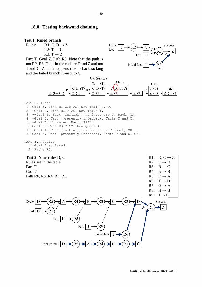
- 80 -
Artificial Intelligence, 18-05-2020
18.8. Testing backward chaining
Test 1. Failed branch
Rules: R1: C, D → Z
R2: T → C
R3: T → Z
Fact T. Goal Z. Path R3. Note that the path is
not R2, R3. Facts in the end are T and Z and not
T and C, Z. This happens due to backtracking
and the failed branch from Z to C.
PART 2. Trace
1) Goal Z. Find R1:C,D->Z. New goals C, D.
2) -Goal C. Find R2:T->C. New goals T.
3) --Goal T. Fact (initial), as facts are T. Back, OK.
4) -Goal C. Fact (presently inferred). Facts T and C.
5) -Goal D. No rules. Back, FAIL.
6) Goal Z. Find R3:T->Z. New goals T.
7) -Goal T. Fact (initial), as facts are T. Back, OK.
8) Goal Z. Fact (presently inferred). Facts T and Z. OK.
PART 3. Results
1) Goal Z achieved.
2) Path: R3.
Test 2. Nine rules D, C R1: D, C → Z
Rules see in the table. R2: C → D
Fact T.
Goal Z.
Path R6, R5, R4, R3, R1.
R3: B → C
R4: A → B
R5: D → A
R6: T → D
R7: G → A
R8: H → B
R9: J → C
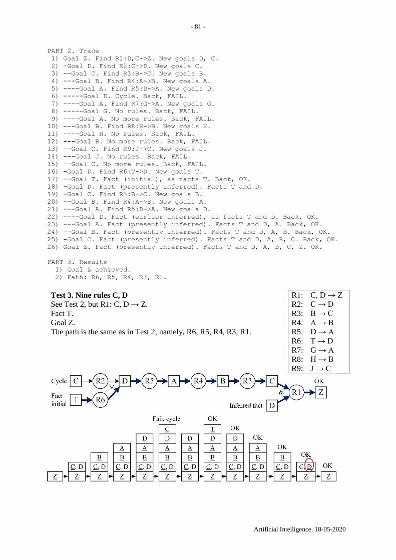
- 81 -
Artificial Intelligence, 18-05-2020
PART 2. Trace
1) Goal Z. Find R1:D,C->Z. New goals D, C.
2) -Goal D. Find R2:C->D. New goals C.
3) --Goal C. Find R3:B->C. New goals B.
4) ---Goal B. Find R4:A->B. New goals A.
5) ----Goal A. Find R5:D->A. New goals D.
6) -----Goal D. Cycle. Back, FAIL.
7) ----Goal A. Find R7:G->A. New goals G.
8) -----Goal G. No rules. Back, FAIL.
9) ----Goal A. No more rules. Back, FAIL.
10) ---Goal B. Find R8:H->B. New goals H.
11) ----Goal H. No rules. Back, FAIL.
12) ---Goal B. No more rules. Back, FAIL.
13) --Goal C. Find R9:J->C. New goals J.
14) ---Goal J. No rules. Back, FAIL.
15) --Goal C. No more rules. Back, FAIL.
16) -Goal D. Find R6:T->D. New goals T.
17) --Goal T. Fact (initial), as facts T. Back, OK.
18) -Goal D. Fact (presently inferred). Facts T and D.
19) -Goal C. Find R3:B->C. New goals B.
20) --Goal B. Find R4:A->B. New goals A.
21) ---Goal A. Find R5:D->A. New goals D.
22) ----Goal D. Fact (earlier inferred), as facts T and D. Back, OK.
23) ---Goal A. Fact (presently inferred). Facts T and D, A. Back, OK.
24) --Goal B. Fact (presently inferred). Facts T and D, A, B. Back, OK.
25) -Goal C. Fact (presently inferred). Facts T and D, A, B, C. Back, OK.
26) Goal Z. Fact (presently inferred). Facts T and D, A, B, C, Z. OK.
PART 3. Results
1) Goal Z achieved.
2) Path: R6, R5, R4, R3, R1.
Test 3. Nine rules C, D R1: C, D → Z
See Test 2, but R1: C, D → Z. R2: C → D
Fact T.
Goal Z.
The path is the same as in Test 2, namely, R6, R5, R4, R3, R1.
R3: B → C
R4: A → B
R5: D → A
R6: T → D
R7: G → A
R8: H → B
R9: J → C
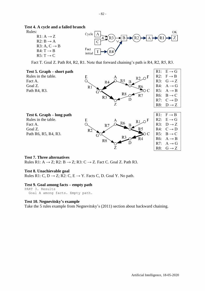
- 82 -
Artificial Intelligence, 18-05-2020
Test 4. A cycle and a failed branch
Rules:
R1: A → Z
R2: B → A
R3: A, C → B
R4: T → B
R5: T → C
Fact T. Goal Z. Path R4, R2, R1. Note that forward chaining’s path is R4, R2, R5, R3.
Test 5. Graph – short path R1: E → G
Rules in the table.
Fact A.
Goal Z.
Path R4, R3.
R2: F → B
R3: G → Z
R4: A → G
R5: A → B
R6: B → C
R7: C → D
R8: D → Z
Test 6. Graph – long path R1: F → B
Rules in the table.
Fact A.
Goal Z.
Path R6, R5, R4, R3.
R2: E → G
R3: D → Z
R4: C → D
R5: B → C
R6: A → B
R7: A → G
R8: G → Z
Test 7. Three alternatives
Rules R1: A → Z; R2: B → Z; R3: C → Z. Fact C. Goal Z. Path R3.
Test 8. Unachievable goal
Rules R1: C, D → Z; R2: C, E → Y. Facts C, D. Goal Y. No path.
Test 9. Goal among facts – empty path PART 3. Results
Goal A among facts. Empty path.
Test 10. Negnevitsky’s example
Take the 5 rules example from Negnevitsky’s (2011) section about backward chaining.
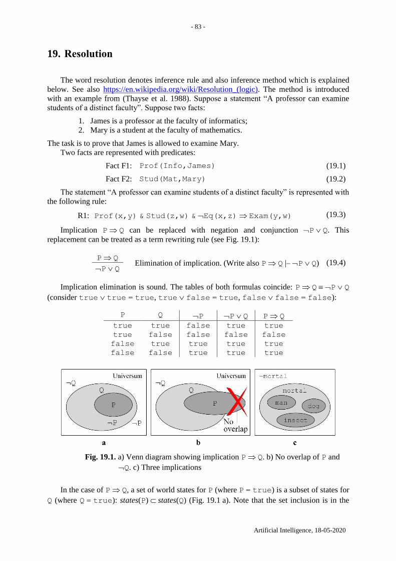
- 83 -
Artificial Intelligence, 18-05-2020
19. Resolution
The word resolution denotes inference rule and also inference method which is explained
below. See also https://en.wikipedia.org/wiki/Resolution_(logic). The method is introduced
with an example from (Thayse et al. 1988). Suppose a statement “A professor can examine
students of a distinct faculty”. Suppose two facts:
1. James is a professor at the faculty of informatics;
2. Mary is a student at the faculty of mathematics.
The task is to prove that James is allowed to examine Mary.
Two facts are represented with predicates:
Fact F1: Prof(Info,James) (19.1)
Fact F2: Stud(Mat,Mary) (19.2)
The statement “A professor can examine students of a distinct faculty” is represented with
the following rule:
R1: Prof(x,y) & Stud(z,w) & Eq(x,z) Exam(y,w) (19.3)
Implication P Q can be replaced with negation and conjunction P Q. This
replacement can be treated as a term rewriting rule (see Fig. 19.1):
P Q Elimination of implication. (Write also P Q |– P Q) (19.4)
P Q
Implication elimination is sound. The tables of both formulas coincide: P Q P Q
(consider true true = true, true false = true, false false = false):
P Q P P Q P Q
true true false true true
true false false false false
false true true true true
false false true true true
Fig. 19.1. a) Venn diagram showing implication P Q. b) No overlap of P and
Q. c) Three implications
In the case of P Q, a set of world states for P (where P = true) is a subset of states for
Q (where Q = true): states(P) states(Q) (Fig. 19.1 a). Note that the set inclusion is in the
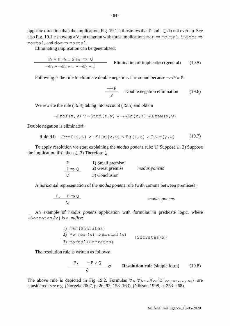
- 84 -
Artificial Intelligence, 18-05-2020
opposite direction than the implication. Fig. 19.1 b illustrates that P and Q do not overlap. See
also Fig. 19.1 c showing a Venn diagram with three implications man mortal, insect
mortal, and dog mortal.
Eliminating implication can be generalised:
P1 & P2 & … & Pn Q Elimination of implication (general) (19.5)
P1 P2 … Pn Q
Following is the rule to eliminate double negation. It is sound because P P:
P Double negation elimination (19.6)
P
We rewrite the rule (19.3) taking into account (19.5) and obtain
Prof(x,y) Stud(z,w) Eq(x,z) Exam(y,w)
Double negation is eliminated:
Rule R1: Prof(x,y) Stud(z,w) Eq(x,z) Exam(y,w) (19.7)
To apply resolution we start explaining the modus ponens rule: 1) Suppose P. 2) Suppose
the implication if P, then Q. 3) Therefore Q.
P 1) Small premise
P Q 2) Great premise modus ponens
Q 3) Conclusion
A horizontal representation of the modus ponens rule (with comma between premises):
P, P Q modus ponens
Q
An example of modus ponens application with formulas in predicate logic, where
{Socrates/x} is a unifier:
1) man(Socrates)
{Socrates/x} 2) x man(x) mortal(x)
3) mortal(Socrates)
The resolution rule is written as follows:
P, P Q Resolution rule (simple form) (19.8)
Q
The above rule is depicted in Fig. 19.2. Formulas x1x2…xn Q(x1,x2,…,xn) are
considered; see e.g. (Norgėla 2007, p. 26, 92, 158–163), (Nilsson 1998, p. 253–268).
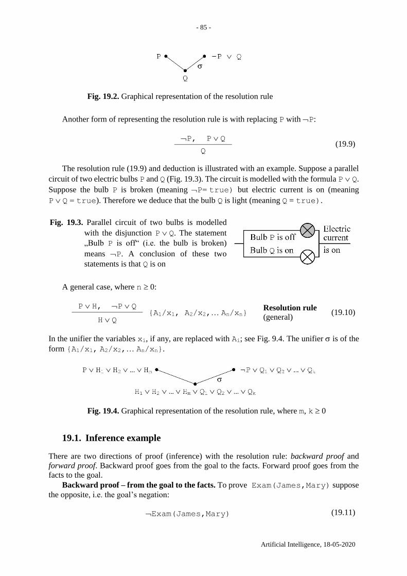
- 85 -
Artificial Intelligence, 18-05-2020
Fig. 19.2. Graphical representation of the resolution rule
Another form of representing the resolution rule is with replacing P with P:
P, P Q (19.9)
Q
The resolution rule (19.9) and deduction is illustrated with an example. Suppose a parallel
circuit of two electric bulbs P and Q (Fig. 19.3). The circuit is modelled with the formula P Q.
Suppose the bulb P is broken (meaning P= true) but electric current is on (meaning
P Q = true). Therefore we deduce that the bulb Q is light (meaning Q = true).
Fig. 19.3. Parallel circuit of two bulbs is modelled
with the disjunction P Q. The statement
„Bulb P is off“ (i.e. the bulb is broken)
means P. A conclusion of these two
statements is that Q is on
A general case, where n 0:
P H, P Q {A1/x1, A2/x2,… An/xn}
Resolution rule
(general) (19.10)
H Q
In the unifier the variables xi, if any, are replaced with Ai; see Fig. 9.4. The unifier is of the
form {A1/x1, A2/x2,… An/xn}.
Fig. 19.4. Graphical representation of the resolution rule, where m, k 0
19.1. Inference example
There are two directions of proof (inference) with the resolution rule: backward proof and
forward proof. Backward proof goes from the goal to the facts. Forward proof goes from the
facts to the goal.
Backward proof – from the goal to the facts. To prove Exam(James,Mary) suppose
the opposite, i.e. the goal’s negation:
Exam(James,Mary) (19.11)
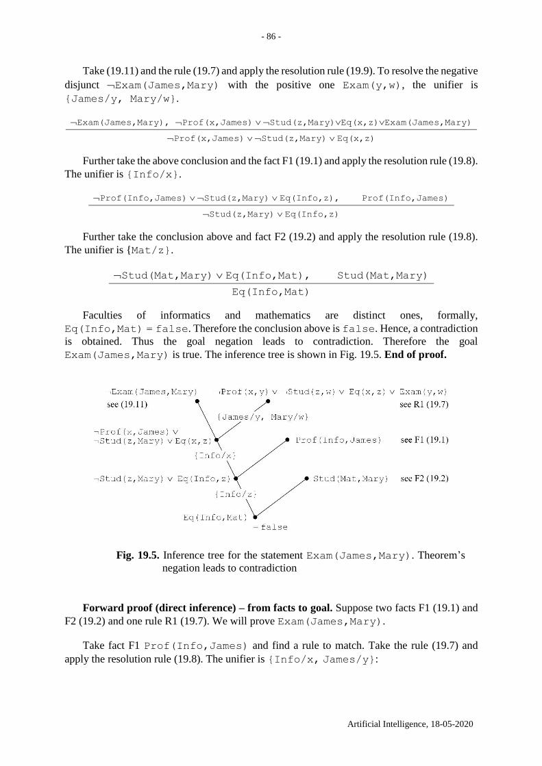
- 86 -
Artificial Intelligence, 18-05-2020
Take (19.11) and the rule (19.7) and apply the resolution rule (19.9). To resolve the negative
disjunct Exam(James,Mary) with the positive one Exam(y,w), the unifier is
{James/y, Mary/w}.
Exam(James,Mary), Prof(x,James) Stud(z,Mary)Eq(x,z)Exam(James,Mary)
Prof(x,James) Stud(z,Mary) Eq(x,z)
Further take the above conclusion and the fact F1 (19.1) and apply the resolution rule (19.8).
The unifier is {Info/x}.
Prof(Info,James) Stud(z,Mary) Eq(Info,z), Prof(Info,James)
Stud(z,Mary) Eq(Info,z)
Further take the conclusion above and fact F2 (19.2) and apply the resolution rule (19.8).
The unifier is {Mat/z}.
Stud(Mat,Mary) Eq(Info,Mat), Stud(Mat,Mary)
Eq(Info,Mat)
Faculties of informatics and mathematics are distinct ones, formally,
Eq(Info,Mat) = false. Therefore the conclusion above is false. Hence, a contradiction
is obtained. Thus the goal negation leads to contradiction. Therefore the goal
Exam(James,Mary) is true. The inference tree is shown in Fig. 19.5. End of proof.
Fig. 19.5. Inference tree for the statement Exam(James,Mary). Theorem’s
negation leads to contradiction
Forward proof (direct inference) – from facts to goal. Suppose two facts F1 (19.1) and
F2 (19.2) and one rule R1 (19.7). We will prove Exam(James,Mary).
Take fact F1 Prof(Info,James) and find a rule to match. Take the rule (19.7) and
apply the resolution rule (19.8). The unifier is {Info/x, James/y}:
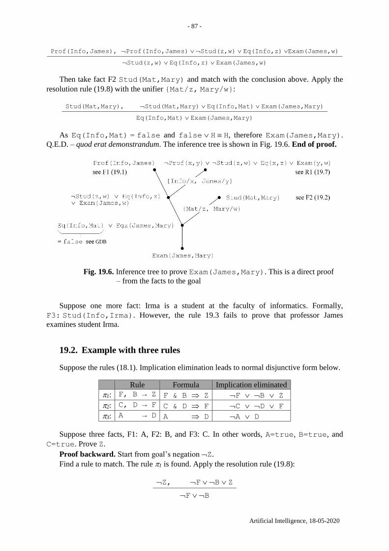
- 87 -
Artificial Intelligence, 18-05-2020
Prof(Info,James), Prof(Info,James) Stud(z,w) Eq(Info,z) Exam(James,w)
Stud(z,w) Eq(Info,z) Exam(James,w)
Then take fact F2 Stud(Mat,Mary) and match with the conclusion above. Apply the
resolution rule (19.8) with the unifier {Mat/z, Mary/w}:
Stud(Mat,Mary), Stud(Mat,Mary) Eq(Info,Mat) Exam(James,Mary)
Eq(Info,Mat) Exam(James,Mary)
As Eq(Info,Mat) = false and false H H, therefore Exam(James,Mary).
Q.E.D. – quod erat demonstrandum. The inference tree is shown in Fig. 19.6. End of proof.
Fig. 19.6. Inference tree to prove Exam(James,Mary). This is a direct proof
– from the facts to the goal
Suppose one more fact: Irma is a student at the faculty of informatics. Formally,
F3: Stud(Info,Irma). However, the rule 19.3 fails to prove that professor James
examines student Irma.
19.2. Example with three rules
Suppose the rules (18.1). Implication elimination leads to normal disjunctive form below.
Rule Formula Implication eliminated
1: F, B → Z F & B Z F B Z
2: C, D → F C & D F C D F
3: A → D A D A D
Suppose three facts, F1: A, F2: B, and F3: C. In other words, A=true, B=true, and
C=true. Prove Z.
Proof backward. Start from goal’s negation Z.
Find a rule to match. The rule 1 is found. Apply the resolution rule (19.8):
Z, F B Z
F B
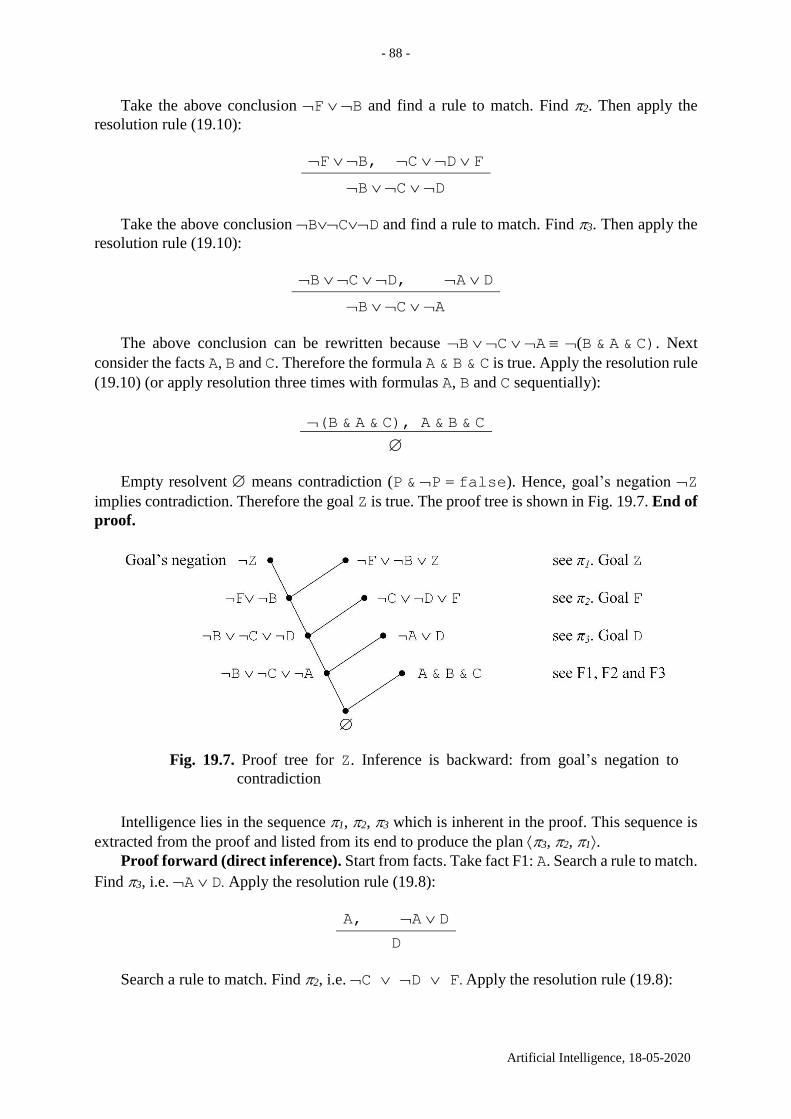
- 88 -
Artificial Intelligence, 18-05-2020
Take the above conclusion F B and find a rule to match. Find 2. Then apply the
resolution rule (19.10):
F B, C D F
B C D
Take the above conclusion BCD and find a rule to match. Find 3. Then apply the
resolution rule (19.10):
B C D, A D
B C A
The above conclusion can be rewritten because B C A (B & A & C). Next
consider the facts A, B and C. Therefore the formula A & B & C is true. Apply the resolution rule
(19.10) (or apply resolution three times with formulas A, B and C sequentially):
(B & A & C), A & B & C
Empty resolvent means contradiction (P & P = false). Hence, goal’s negation Z
implies contradiction. Therefore the goal Z is true. The proof tree is shown in Fig. 19.7. End of
proof.
Fig. 19.7. Proof tree for Z. Inference is backward: from goal’s negation to
contradiction
Intelligence lies in the sequence 1, 2, 3 which is inherent in the proof. This sequence is
extracted from the proof and listed from its end to produce the plan 3, 2, 1.
Proof forward (direct inference). Start from facts. Take fact F1: A. Search a rule to match.
Find 3, i.e. A D. Apply the resolution rule (19.8):
A, A D
D
Search a rule to match. Find 2, i.e. C D F. Apply the resolution rule (19.8):
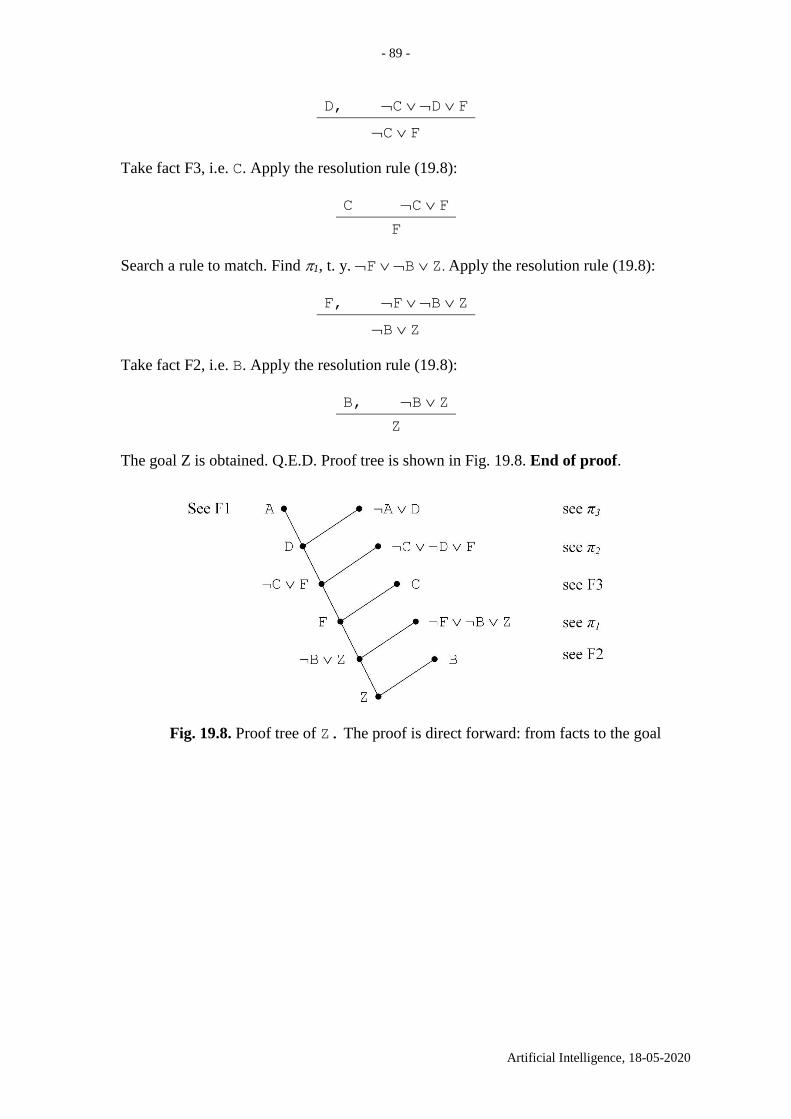
- 89 -
Artificial Intelligence, 18-05-2020
D, C D F
C F
Take fact F3, i.e. C. Apply the resolution rule (19.8):
C C F
F
Search a rule to match. Find 1, t. y. F B Z. Apply the resolution rule (19.8):
F, F B Z
B Z
Take fact F2, i.e. B. Apply the resolution rule (19.8):
B, B Z
Z
The goal Z is obtained. Q.E.D. Proof tree is shown in Fig. 19.8. End of proof.
Fig. 19.8. Proof tree of Z. The proof is direct forward: from facts to the goal
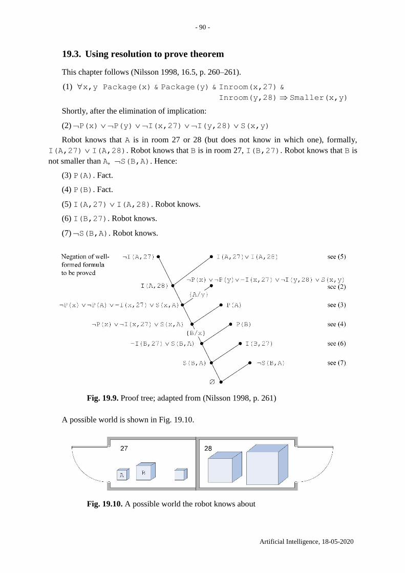
- 90 -
Artificial Intelligence, 18-05-2020
19.3. Using resolution to prove theorem
This chapter follows (Nilsson 1998, 16.5, p. 260–261).
(1) x,y Package(x) & Package(y) & Inroom(x,27) &
Inroom(y,28) Smaller(x,y)
Shortly, after the elimination of implication:
(2) P(x) P(y) I(x,27) I(y,28) S(x,y)
Robot knows that A is in room 27 or 28 (but does not know in which one), formally,
I(A,27) I(A,28). Robot knows that B is in room 27, I(B,27). Robot knows that B is
not smaller than A, S(B,A). Hence:
(3) P(A). Fact.
(4) P(B). Fact.
(5) I(A,27) I(A,28). Robot knows.
(6) I(B,27). Robot knows.
(7) S(B,A). Robot knows.
Fig. 19.9. Proof tree; adapted from (Nilsson 1998, p. 261)
A possible world is shown in Fig. 19.10.
Fig. 19.10. A possible world the robot knows about
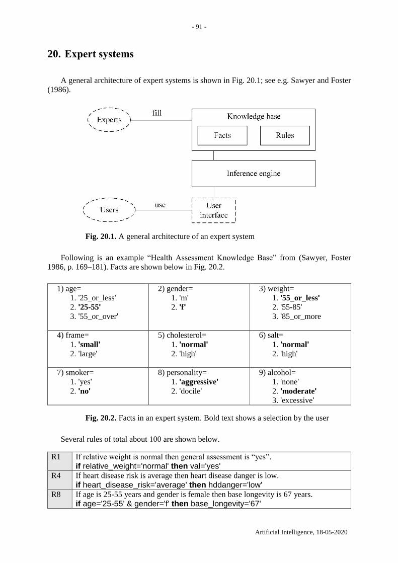
- 91 -
Artificial Intelligence, 18-05-2020
20. Expert systems
A general architecture of expert systems is shown in Fig. 20.1; see e.g. Sawyer and Foster
(1986).
Fig. 20.1. A general architecture of an expert system
Following is an example “Health Assessment Knowledge Base” from (Sawyer, Foster
1986, p. 169–181). Facts are shown below in Fig. 20.2.
1) age=
1. '25_or_less' 2. '25-55' 3. '55_or_over'
2) gender=
1. 'm' 2. 'f'
3) weight=
1. '55_or_less' 2. '55-85' 3. '85_or_more
4) frame=
1. 'small' 2. 'large'
5) cholesterol=
1. 'normal' 2. 'high'
6) salt=
1. 'normal' 2. 'high'
7) smoker=
1. 'yes' 2. 'no'
8) personality=
1. 'aggressive' 2. 'docile'
9) alcohol=
1. 'none' 2. 'moderate' 3. 'excessive'
Fig. 20.2. Facts in an expert system. Bold text shows a selection by the user
Several rules of total about 100 are shown below.
R1 If relative weight is normal then general assessment is “yes”.
if relative_weight='normal' then val='yes' R4 If heart disease risk is average then heart disease danger is low.
if heart_disease_risk='average' then hddanger='low' R8 If age is 25-55 years and gender is female then base longevity is 67 years.
if age='25-55' & gender='f' then base_longevity='67'
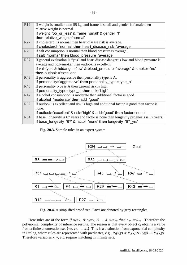
- 92 -
Artificial Intelligence, 18-05-2020
R12 If weight is smaller than 55 kg, and frame is small and gender is female then
relative weight is normal.
if weight='55_or_less' & frame='small' & gender='f' then relative_weight='normal'
R27 If cholesterol is normal then heart disease risk is average.
if cholesterol='normal' then heart_disease_risk='average' R29 If salt consumption is normal then blood pressure is average.
if salt='normal' then blood_pressure='average'
R37 If general evaluation is “yes” and heart disease danger is low and blood pressure is
average and non-smoker then outlook is excellent.
if val='yes' & hddanger='low' & blood_pressure='average' & smoker='no' then outlook ='excellent'
R43 If personality is aggressive then personality type is A.
if personality='aggressive' then personality_type='type_a' R45 If personality type is A then general risk is high.
if personality_type='type_a' then risk='high' R47 If alcohol consumption is moderate then additional factor is good.
if alcohol='moderate' then add='good' R52 If outlook is excellent and risk is high and additional factor is good then factor is
none.
if outlook='excellent' & risk='high' & add='good' then factor='none' R64 If base_longevity is 67 years and factor is none then longevity prognosis is 67 years.
if base_longevity='67' & factor='none' then longevity='67_yrs'
Fig. 20.3. Sample rules in an expert system
Fig. 20.4. A simplified proof tree. Facts are denoted by grey rectangles
Here rules are of the form if o1=v1 & o2=v2 & … & on=vn then on+1=vn+1 . Therefore the
polynomial complexity of inference results. The reason is that every object oi obtains a value
from a finite enumeration set {vi1, vi2, …,vim}. This is a distinction from exponential complexity
in Prolog, where rules are represented with predicates, e.g., P1(x,y) & P2(x) & P3(y) → P4(x,y).
Therefore variables x, y, etc. require matching in infinite sets.
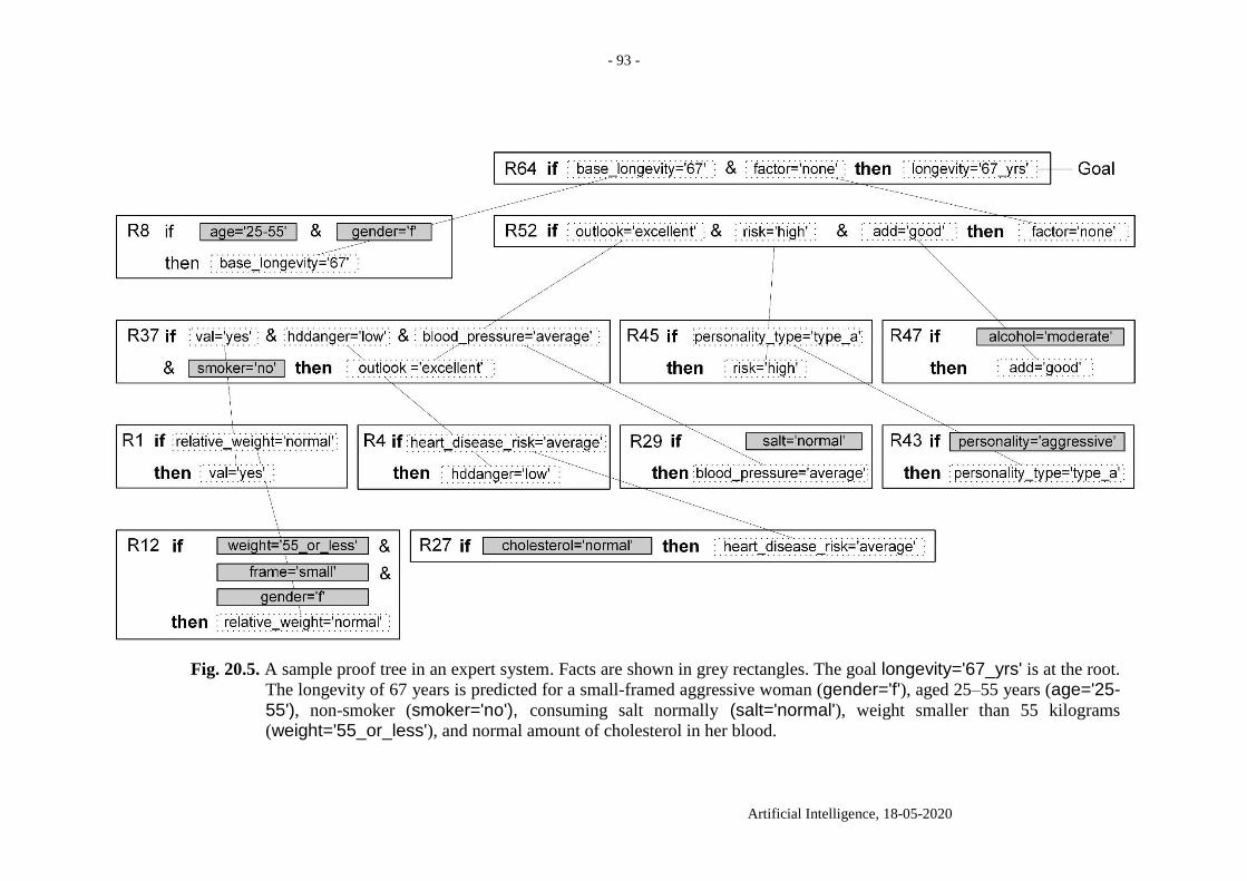
- 93 -
Artificial Intelligence, 18-05-2020
Fig. 20.5. A sample proof tree in an expert system. Facts are shown in grey rectangles. The goal longevity='67_yrs' is at the root.
The longevity of 67 years is predicted for a small-framed aggressive woman (gender='f'), aged 25–55 years (age='25-55'), non-smoker (smoker='no'), consuming salt normally (salt='normal'), weight smaller than 55 kilograms
(weight='55_or_less'), and normal amount of cholesterol in her blood.
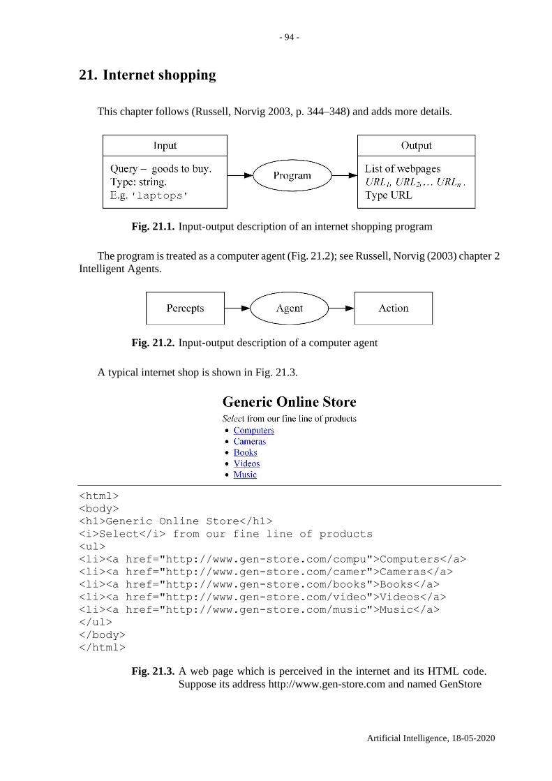
- 94 -
Artificial Intelligence, 18-05-2020
21. Internet shopping
This chapter follows (Russell, Norvig 2003, p. 344–348) and adds more details.
Fig. 21.1. Input-output description of an internet shopping program
The program is treated as a computer agent (Fig. 21.2); see Russell, Norvig (2003) chapter 2
Intelligent Agents.
Fig. 21.2. Input-output description of a computer agent
A typical internet shop is shown in Fig. 21.3.
<html>
<body>
<h1>Generic Online Store</h1>
<i>Select</i> from our fine line of products
<ul>
<li><a href="http://www.gen-store.com/compu">Computers</a>
<li><a href="http://www.gen-store.com/camer">Cameras</a>
<li><a href="http://www.gen-store.com/books">Books</a>
<li><a href="http://www.gen-store.com/video">Videos</a>
<li><a href="http://www.gen-store.com/music">Music</a>
</ul>
</body>
</html>
Fig. 21.3. A web page which is perceived in the internet and its HTML code.
Suppose its address http://www.gen-store.com and named GenStore
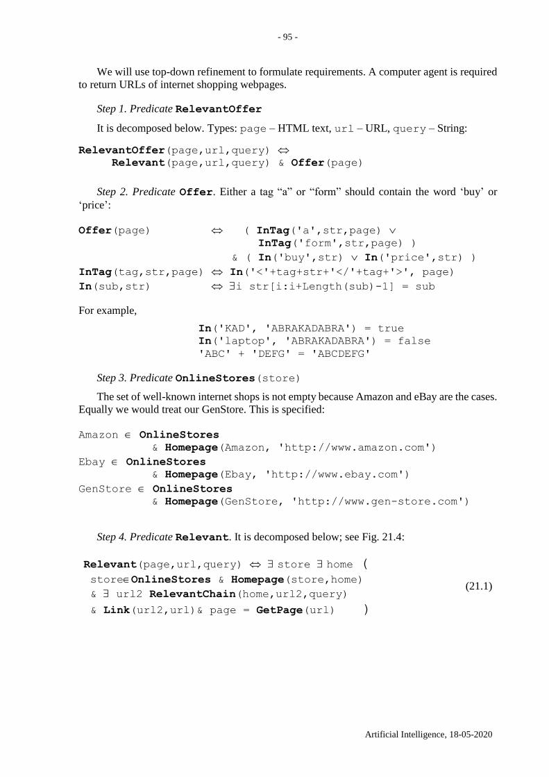
- 95 -
Artificial Intelligence, 18-05-2020
We will use top-down refinement to formulate requirements. A computer agent is required
to return URLs of internet shopping webpages.
Step 1. Predicate RelevantOffer
It is decomposed below. Types: page – HTML text, url – URL, query – String:
RelevantOffer(page,url,query)
Relevant(page,url,query) & Offer(page)
Step 2. Predicate Offer. Either a tag “a” or “form” should contain the word ‘buy’ or
‘price’:
Offer(page) ( InTag('a',str,page)
InTag('form',str,page) )
& ( In('buy',str) In('price',str) )
InTag(tag,str,page) In('<'+tag+str+'</'+tag+'>', page)
In(sub,str) i str[i:i+Length(sub)-1] = sub
For example,
In('KAD', 'ABRAKADABRA') = true
In('laptop', 'ABRAKADABRA') = false
'ABC' + 'DEFG' = 'ABCDEFG'
Step 3. Predicate OnlineStores(store)
The set of well-known internet shops is not empty because Amazon and eBay are the cases.
Equally we would treat our GenStore. This is specified:
Amazon OnlineStores
& Homepage(Amazon, 'http://www.amazon.com')
Ebay OnlineStores & Homepage(Ebay, 'http://www.ebay.com')
GenStore OnlineStores & Homepage(GenStore, 'http://www.gen-store.com')
Step 4. Predicate Relevant. It is decomposed below; see Fig. 21.4:
Relevant(page,url,query) store home (
storeOnlineStores & Homepage(store,home)
& url2 RelevantChain(home,url2,query)
& Link(url2,url)& page = GetPage(url) )
(21.1)
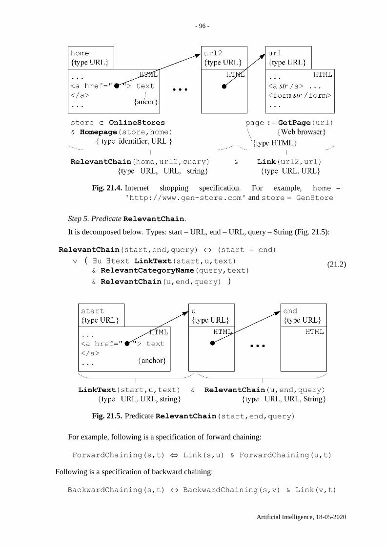
- 96 -
Artificial Intelligence, 18-05-2020
Fig. 21.4. Internet shopping specification. For example, home =
'http://www.gen-store.com' and store = GenStore
Step 5. Predicate RelevantChain.
It is decomposed below. Types: start – URL, end – URL, query – String (Fig. 21.5):
RelevantChain(start,end,query) (start = end)
( u text LinkText(start,u,text) & RelevantCategoryName(query,text)
& RelevantChain(u,end,query) )
(21.2)
Fig. 21.5. Predicate RelevantChain(start,end,query)
For example, following is a specification of forward chaining:
ForwardChaining(s,t) Link(s,u) & ForwardChaining(u,t)
Following is a specification of backward chaining:
BackwardChaining(s,t) BackwardChaining(s,v) & Link(v,t)
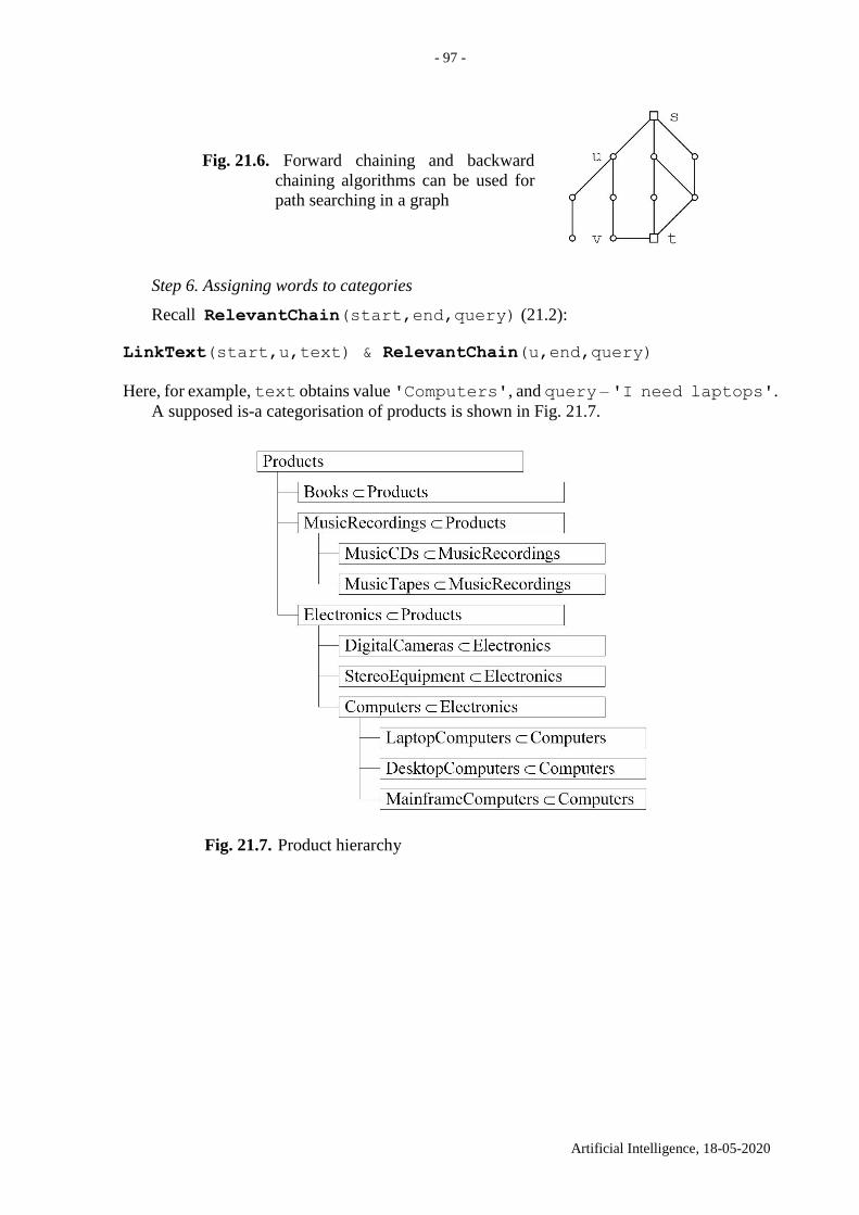
- 97 -
Artificial Intelligence, 18-05-2020
Fig. 21.6. Forward chaining and backward
chaining algorithms can be used for
path searching in a graph
Step 6. Assigning words to categories
Recall RelevantChain(start,end,query) (21.2):
LinkText(start,u,text) & RelevantChain(u,end,query)
Here, for example, text obtains value 'Computers', and query – 'I need laptops'.
A supposed is-a categorisation of products is shown in Fig. 21.7.
Fig. 21.7. Product hierarchy
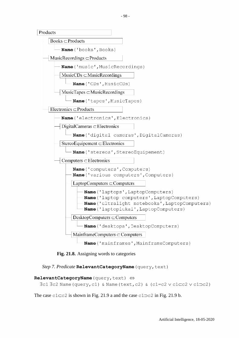
- 98 -
Artificial Intelligence, 18-05-2020
Fig. 21.8. Assigning words to categories
Step 7. Predicate RelevantCategoryName(query,text)
RelevantCategoryName(query,text)
c1 c2 Name(query,c1) & Name(text,c2) & (c1=c2 c1c2 c1c2)
The case c1c2 is shown in Fig. 21.9 a and the case c1c2 in Fig. 21.9 b.
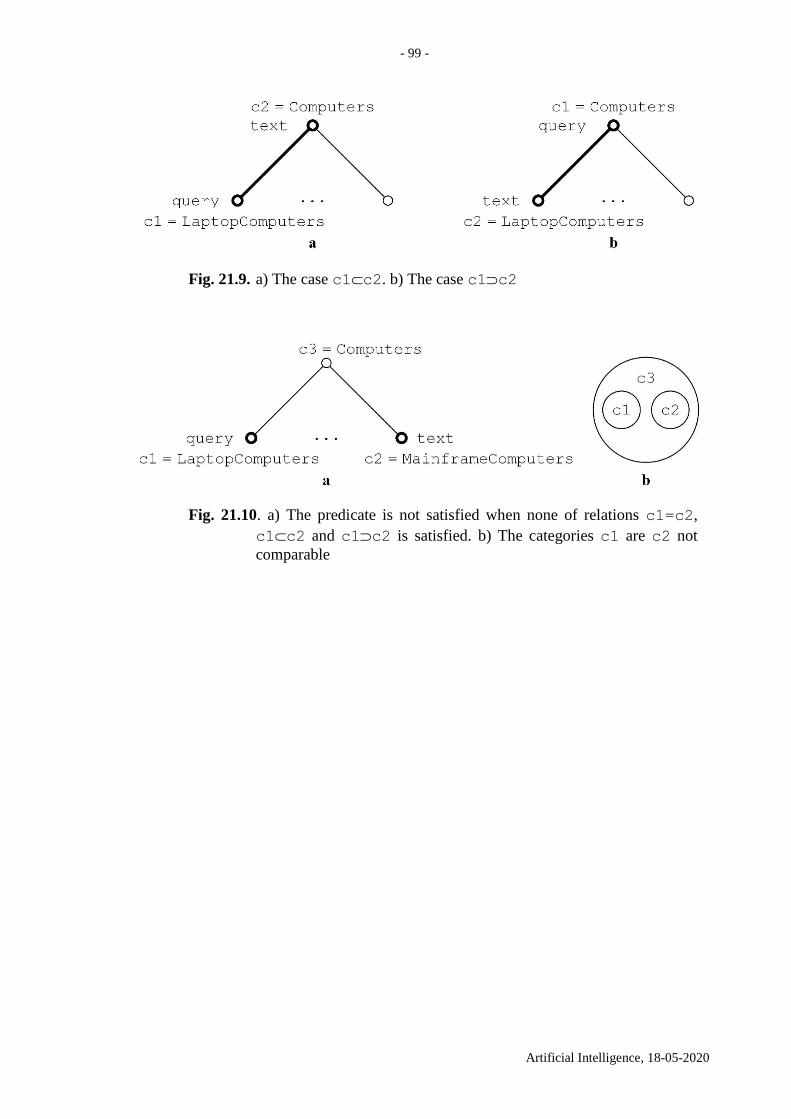
- 99 -
Artificial Intelligence, 18-05-2020
Fig. 21.9. a) The case c1c2. b) The case c1c2
Fig. 21.10. a) The predicate is not satisfied when none of relations c1=c2,
c1c2 and c1c2 is satisfied. b) The categories c1 are c2 not
comparable
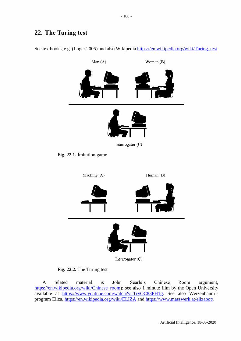
- 100 -
Artificial Intelligence, 18-05-2020
22. The Turing test
See textbooks, e.g. (Luger 2005) and also Wikipedia https://en.wikipedia.org/wiki/Turing_test.
Fig. 22.1. Imitation game
Fig. 22.2. The Turing test
A related material is John Searle’s Chinese Room argument,
https://en.wikipedia.org/wiki/Chinese_room); see also 1 minute film by the Open University
available at https://www.youtube.com/watch?v=TryOC83PH1g. See also Weizenbaum’s
program Eliza, https://en.wikipedia.org/wiki/ELIZA and https://www.masswerk.at/elizabot/.
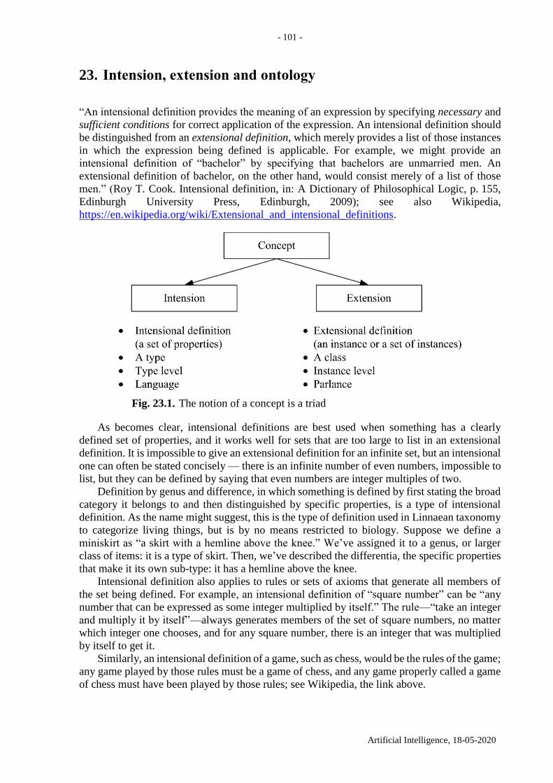
- 101 -
Artificial Intelligence, 18-05-2020
23. Intension, extension and ontology
“An intensional definition provides the meaning of an expression by specifying necessary and
sufficient conditions for correct application of the expression. An intensional definition should
be distinguished from an extensional definition, which merely provides a list of those instances
in which the expression being defined is applicable. For example, we might provide an
intensional definition of “bachelor” by specifying that bachelors are unmarried men. An
extensional definition of bachelor, on the other hand, would consist merely of a list of those
men.” (Roy T. Cook. Intensional definition, in: A Dictionary of Philosophical Logic, p. 155,
Edinburgh University Press, Edinburgh, 2009); see also Wikipedia,
https://en.wikipedia.org/wiki/Extensional_and_intensional_definitions.
Fig. 23.1. The notion of a concept is a triad
As becomes clear, intensional definitions are best used when something has a clearly
defined set of properties, and it works well for sets that are too large to list in an extensional
definition. It is impossible to give an extensional definition for an infinite set, but an intensional
one can often be stated concisely — there is an infinite number of even numbers, impossible to
list, but they can be defined by saying that even numbers are integer multiples of two.
Definition by genus and difference, in which something is defined by first stating the broad
category it belongs to and then distinguished by specific properties, is a type of intensional
definition. As the name might suggest, this is the type of definition used in Linnaean taxonomy
to categorize living things, but is by no means restricted to biology. Suppose we define a
miniskirt as “a skirt with a hemline above the knee.” We’ve assigned it to a genus, or larger
class of items: it is a type of skirt. Then, we’ve described the differentia, the specific properties
that make it its own sub-type: it has a hemline above the knee.
Intensional definition also applies to rules or sets of axioms that generate all members of
the set being defined. For example, an intensional definition of “square number” can be “any
number that can be expressed as some integer multiplied by itself.” The rule—“take an integer
and multiply it by itself”—always generates members of the set of square numbers, no matter
which integer one chooses, and for any square number, there is an integer that was multiplied
by itself to get it.
Similarly, an intensional definition of a game, such as chess, would be the rules of the game;
any game played by those rules must be a game of chess, and any game properly called a game
of chess must have been played by those rules; see Wikipedia, the link above.
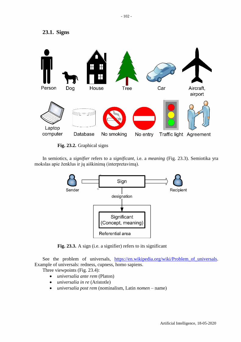
- 102 -
Artificial Intelligence, 18-05-2020
23.1. Signs
Fig. 23.2. Graphical signs
In semiotics, a signifier refers to a significant, i.e. a meaning (Fig. 23.3). Semiotika yra
mokslas apie ženklus ir jų aiškinimą (interpretavimą).
Fig. 23.3. A sign (i.e. a signifier) refers to its significant
See the problem of universals, https://en.wikipedia.org/wiki/Problem_of_universals.
Example of universals: redness, cupness, homo sapiens.
Three viewpoints (Fig. 23.4):
universalia ante rem (Platon)
universalia in re (Aristotle)
universalia post rem (nominalism, Latin nomen – name)
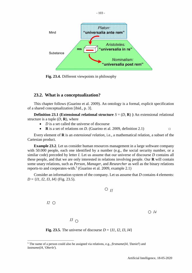
- 103 -
Artificial Intelligence, 18-05-2020
Fig. 23.4. Different viewpoints in philosophy
23.2. What is a conceptualization?
This chapter follows (Guarino et al. 2009). An ontology is a formal, explicit specification
of a shared conceptualization [ibid., p. 3].
Definition 23.1 (Extensional relational structure S = (D, R) ) An extensional relational
structure is a tuple (D, R), where
D is a set called the universe of discourse
R is a set of relations on D. (Guarino et al. 2009, definition 2.1) □
Every element of R is an extensional relation, i.e., a mathematical relation, a subset of the
Cartesian product.
Example 23.2. Let us consider human resources management in a large software company
with 50.000 people, each one identified by a number (e.g., the social security number, or a
similar code) preceded by letter I. Let us assume that our universe of discourse D contains all
these people, and that we are only interested in relations involving people. Our R will contain
some unary relations, such as Person, Manager, and Researcher as well as the binary relations
reports-to and cooperates-with.5 (Guarino et al. 2009, example 2.1)
Consider an information system of the company. Let us assume that D contains 4 elements:
D = {I1, I2, I3, I4} (Fig. 23.5).
Fig. 23.5. The universe of discourse D = {I1, I2, I3, I4}
5 The name of a person could also be assigned via relations, e.g., firstname(I4, 'Daniel') and
lastname(I4, 'Oberle').
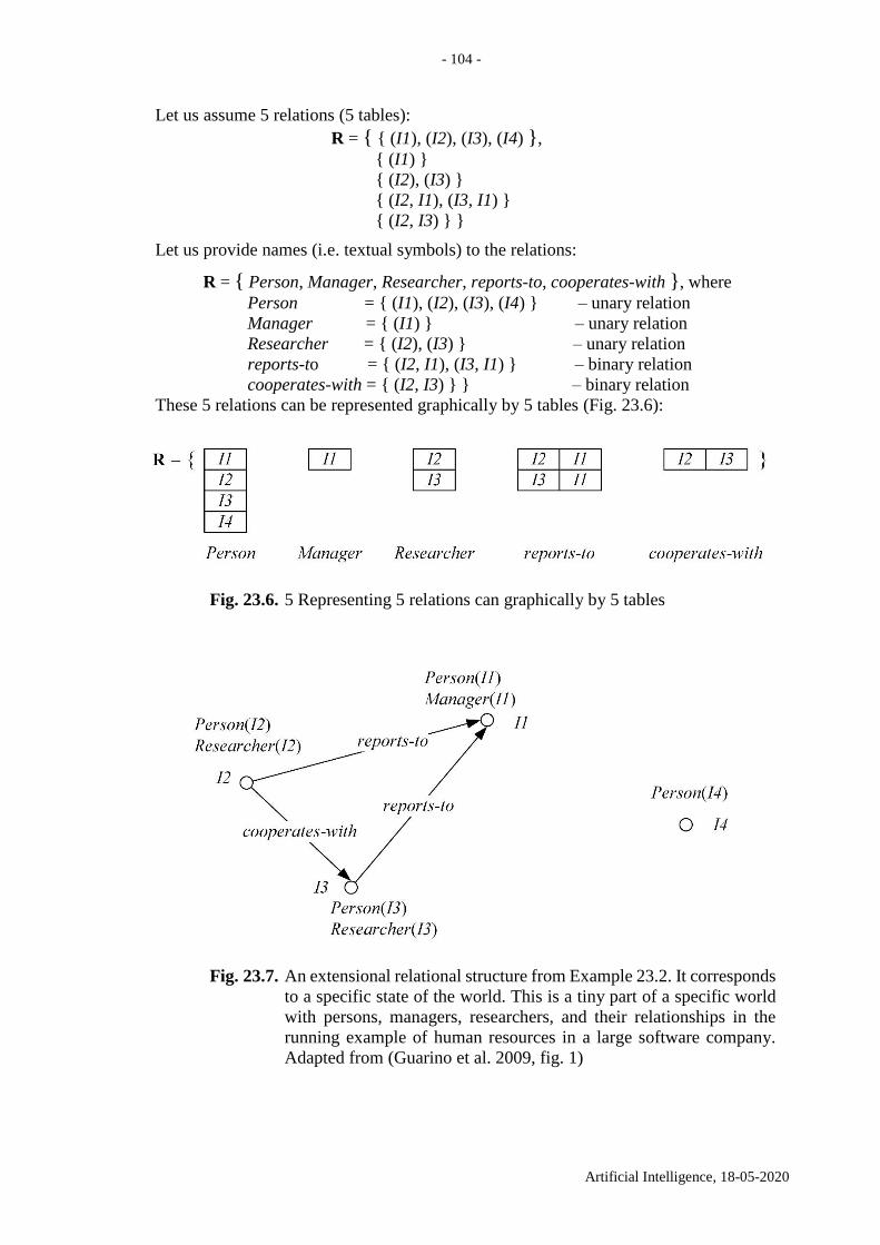
- 104 -
Artificial Intelligence, 18-05-2020
Let us assume 5 relations (5 tables):
R = { { (I1), (I2), (I3), (I4) },
{ (I1) }
{ (I2), (I3) }
{ (I2, I1), (I3, I1) }
{ (I2, I3) } }
Let us provide names (i.e. textual symbols) to the relations:
R = { Person, Manager, Researcher, reports-to, cooperates-with }, where
Person = { (I1), (I2), (I3), (I4) } – unary relation
Manager = { (I1) } – unary relation
Researcher = { (I2), (I3) } – unary relation
reports-to = { (I2, I1), (I3, I1) } – binary relation
cooperates-with = { (I2, I3) } } – binary relation
These 5 relations can be represented graphically by 5 tables (Fig. 23.6):
Fig. 23.6. 5 Representing 5 relations can graphically by 5 tables
Fig. 23.7. An extensional relational structure from Example 23.2. It corresponds
to a specific state of the world. This is a tiny part of a specific world
with persons, managers, researchers, and their relationships in the
running example of human resources in a large software company.
Adapted from (Guarino et al. 2009, fig. 1)
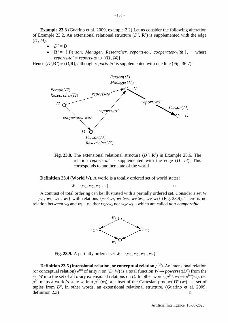
- 105 -
Artificial Intelligence, 18-05-2020
Example 23.3 (Guarino et al. 2009, example 2.2) Let us consider the following alteration
of Example 23.2. An extensional relational structure (D’, R’) is supplemented with the edge
(I1, I4):
D’ = D
R’ = { Person, Manager, Researcher, reports-to’, cooperates-with }, where
reports-to’ = reports-to {(I1, I4)}
Hence (D’,R’) (D,R), although reports-to’ is supplemented with one line (Fig. 36.7).
Fig. 23.8. The extensional relational structure (D’, R’) in Example 23.6. The
relation reports-to’ is supplemented with the edge (I1, I4). This
corresponds to another state of the world
Definition 23.4 (World W). A world is a totally ordered set of world states:
W = {w1, w2, w3 …} □
A contrast of total ordering can be illustrated with a partially ordered set. Consider a set W
= {w1, w2, w3 , w4} with relations {w1<w2, w1<w3, w2<w4, w3<w4} (Fig. 23.9). There is no
relation between w2 and w3 – neither w2<w3 nor w2>w3 – which are called non-comparable.
Fig. 23.9. A partially ordered set W = {w1, w2, w3 , w4}
Definition 23.5 (Intensional relation, or conceptual relation ρ(n)). An intensional relation
(or conceptual relation) ρ(n) of arity n on (D, W) is a total function W → powerset(Dn) from the
set W into the set of all n-ary extensional relations on D. In other words, ρ(n): wi → ρ(n)(wi), i.e.
ρ(n) maps a world’s state wi into ρ(n)(wi), a subset of the Cartesian product Dn (wi) – a set of
tuples from Dn, in other words, an extensional relational structure. (Guarino et al. 2009,
definition 2.3) □
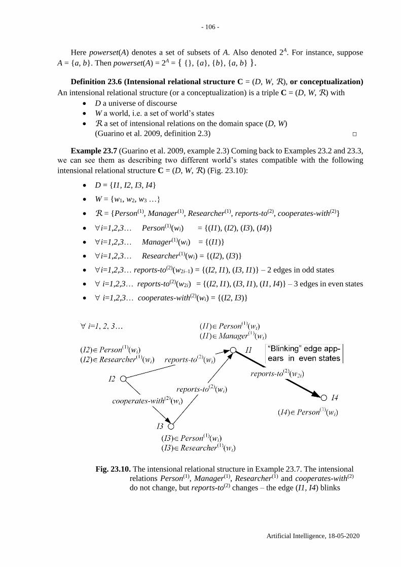
- 106 -
Artificial Intelligence, 18-05-2020
Here powerset(A) denotes a set of subsets of A. Also denoted 2A. For instance, suppose
A = {a, b}. Then powerset(A) = 2A = { {}, {a}, {b}, {a, b} }.
Definition 23.6 (Intensional relational structure C = (D, W, R), or conceptualization)
An intensional relational structure (or a conceptualization) is a triple C = (D, W, R) with
D a universe of discourse
W a world, i.e. a set of world’s states
R a set of intensional relations on the domain space (D, W)
(Guarino et al. 2009, definition 2.3) □
Example 23.7 (Guarino et al. 2009, example 2.3) Coming back to Examples 23.2 and 23.3,
we can see them as describing two different world’s states compatible with the following
intensional relational structure C = (D, W, R) (Fig. 23.10):
D = {I1, I2, I3, I4}
W = {w1, w2, w3 …}
R = {Person(1), Manager(1), Researcher(1), reports-to(2), cooperates-with(2)}
i=1,2,3… Person(1)(wi) = {(I1), (I2), (I3), (I4)}
i=1,2,3… Manager(1)(wi) = {(I1)}
i=1,2,3… Researcher(1)(wi) = {(I2), (I3)}
i=1,2,3… reports-to(2)(w2i–1) = {(I2, I1), (I3, I1)} – 2 edges in odd states
i=1,2,3… reports-to(2)(w2i) = {(I2, I1), (I3, I1), (I1, I4)} – 3 edges in even states
i=1,2,3… cooperates-with(2)(wi) = {(I2, I3)}
Fig. 23.10. The intensional relational structure in Example 23.7. The intensional
relations Person(1), Manager(1), Researcher(1) and cooperates-with(2)
do not change, but reports-to(2) changes – the edge (I1, I4) blinks
- 107 -
Artificial Intelligence, 18-05-2020
23.3. What is a proper formal, explicit specification?
In practical applications, as well as in human communication, we need to use a language to
refer to the elements of a conceptualization: for instance, to express the fact that I2 cooperates
with I3, we have to introduce a specific symbol (formally, a predicate symbol, say 'cooperates-
with', which, in the user’s intention, is intended to represent a certain conceptual relation. We
say in this case that our language (let us call it L) commits to a conceptualization. Suppose now
that L is a first-order logical language, whose non-logical symbols (i.e., its vocabulary) is V.
The vocabulary is divided into two sets: 1) constant symbols, e.g, 'I1', 'I2', 'I3', 'I4', and
2) predicate symbols, e.g., 'Person', 'Manager', 'Researcher', 'reports-to', 'cooperates-with':
V = constant symbols predicate symbols
A first-order language has the following difference from higher-order languages: predicate
arguments can be formed of variables and expressions, but not of predicate names. In other
words, a table field cannot be a table’s name. Examples of correct first-order sentences are
'reports-to'('I2', 'I1') = 'true' and x,y 'reports-to'(x,y) 'Person'(x) & 'Person'(y), but not
'reports-to'('Person', 'Person').
Definition 23.8 (Extensional first-order structure M = (S, I ) ). Let us assume
L a first-order logical language with vocabulary V
S = (D, R) an extensional relational structure
An extensional first-order structure (also called model for L) is a tuple M = (S, I ), where I
(called extensional interpretation function) is a total function I: V → D R that maps each
vocabulary symbol of V to either an element of D or an extensional relation belonging to the
set R. In other words, I maps constant symbols to D and predicate symbols to R, where
S = (D, R). (Guarino et al. 2009, definition 3.1) □
Definition 23.9 (Intensional first-order structure K= (C, I ), also called ontological
commitment). Let us assume
L a first-order logical language with vocabulary V
C = (D, W, R) an intensional relational structure (conceptualization)
An intensional first-order structure (also called ontological commitment) for L is a tuple
K= (C, I ), where kur I (called intensional interpretation function) is a total function I :
V → D R , that maps each vocabulary symbol of V to either an element of D or an
intensional relation belonging to the set R. In other words, I maps constant symbols to D and
predicate symbols to R , where C = (D, W, R). (Guarino et al. 2009, definition 3.2) □
Example 23.10 (Guarino et al. 2009, example 3.1) Let us come back to the extensional
relational structure in our Example 23.2. An intensional first-order structure is as follows:
V = {'I1', 'I2', 'I3', 'I4'}
{'Person', 'Manager', 'Researcher', 'reports-to', 'cooperates-with'}
I : 'I1' → I1, 'I2' → I2, 'I3' → I3, 'I4' → I4,
'Person' → Person(1) , 'Manager' → Manager(1), 'Researcher' → Researcher(1),
'reports-to' → reports-to(2), 'cooperates-with'→ cooperates-with(2)
Definition 23.11 (Intended models IK(L) ). Let us assume
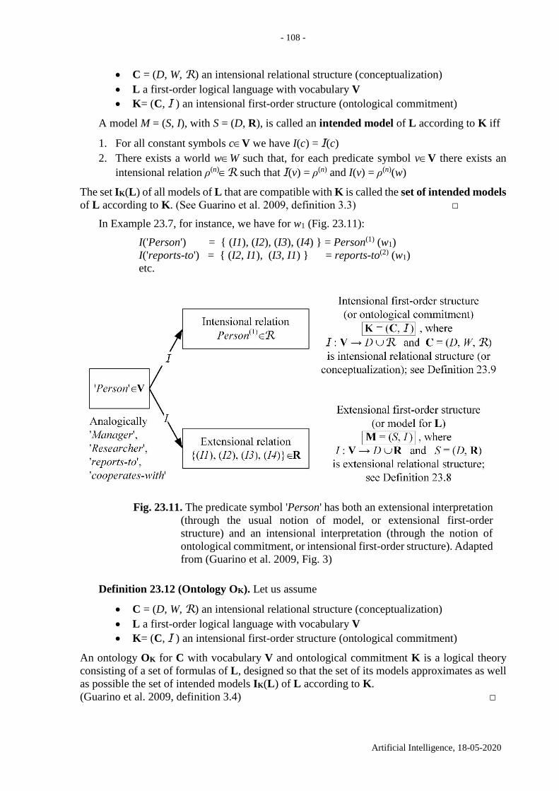
- 108 -
Artificial Intelligence, 18-05-2020
C = (D, W, R) an intensional relational structure (conceptualization)
L a first-order logical language with vocabulary V
K= (C, I ) an intensional first-order structure (ontological commitment)
A model M = (S, I), with S = (D, R), is called an intended model of L according to K iff
1. For all constant symbols cV we have I(c) = I(c)
2. There exists a world wW such that, for each predicate symbol vV there exists an
intensional relation ρ(n)R such that I(v) = ρ(n) and I(v) = ρ(n)(w)
The set IK(L) of all models of L that are compatible with K is called the set of intended models
of L according to K. (See Guarino et al. 2009, definition 3.3) □
In Example 23.7, for instance, we have for w1 (Fig. 23.11):
I('Person') = { (I1), (I2), (I3), (I4) } = Person(1) (w1)
I('reports-to') = { (I2, I1), (I3, I1) } = reports-to(2) (w1)
etc.
Fig. 23.11. The predicate symbol 'Person' has both an extensional interpretation
(through the usual notion of model, or extensional first-order
structure) and an intensional interpretation (through the notion of
ontological commitment, or intensional first-order structure). Adapted
from (Guarino et al. 2009, Fig. 3)
Definition 23.12 (Ontology OK). Let us assume
C = (D, W, R) an intensional relational structure (conceptualization)
L a first-order logical language with vocabulary V
K= (C, I ) an intensional first-order structure (ontological commitment)
An ontology OK for C with vocabulary V and ontological commitment K is a logical theory
consisting of a set of formulas of L, designed so that the set of its models approximates as well
as possible the set of intended models IK(L) of L according to K.
(Guarino et al. 2009, definition 3.4) □
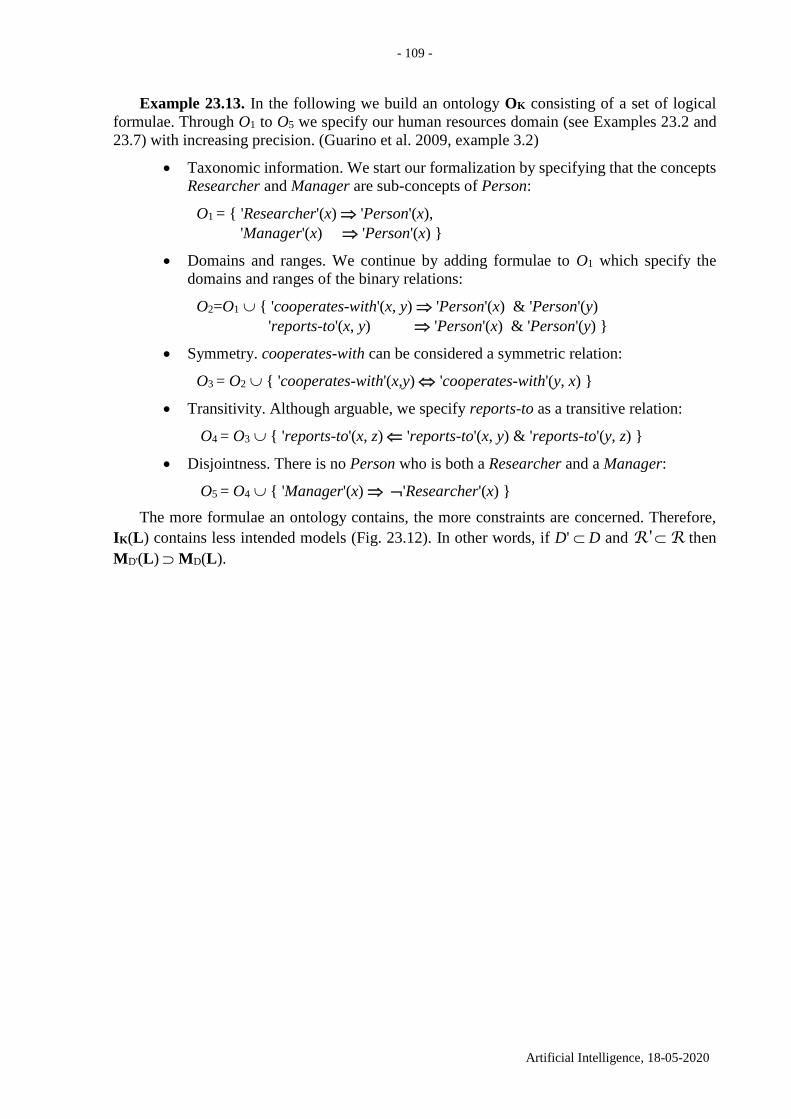
- 109 -
Artificial Intelligence, 18-05-2020
Example 23.13. In the following we build an ontology OK consisting of a set of logical
formulae. Through O1 to O5 we specify our human resources domain (see Examples 23.2 and
23.7) with increasing precision. (Guarino et al. 2009, example 3.2)
Taxonomic information. We start our formalization by specifying that the concepts
Researcher and Manager are sub-concepts of Person:
O1 = { 'Researcher'(x) 'Person'(x),
'Manager'(x) 'Person'(x) }
Domains and ranges. We continue by adding formulae to O1 which specify the
domains and ranges of the binary relations:
O2=O1 { 'cooperates-with'(x, y) 'Person'(x) & 'Person'(y)
'reports-to'(x, y) 'Person'(x) & 'Person'(y) }
Symmetry. cooperates-with can be considered a symmetric relation:
O3 = O2 { 'cooperates-with'(x,y) 'cooperates-with'(y, x) }
Transitivity. Although arguable, we specify reports-to as a transitive relation:
O4 = O3 { 'reports-to'(x, z) 'reports-to'(x, y) & 'reports-to'(y, z) }
Disjointness. There is no Person who is both a Researcher and a Manager:
O5 = O4 { 'Manager'(x) 'Researcher'(x) }
The more formulae an ontology contains, the more constraints are concerned. Therefore,
IK(L) contains less intended models (Fig. 23.12). In other words, if D' D and R' R then
MD'(L) MD(L).
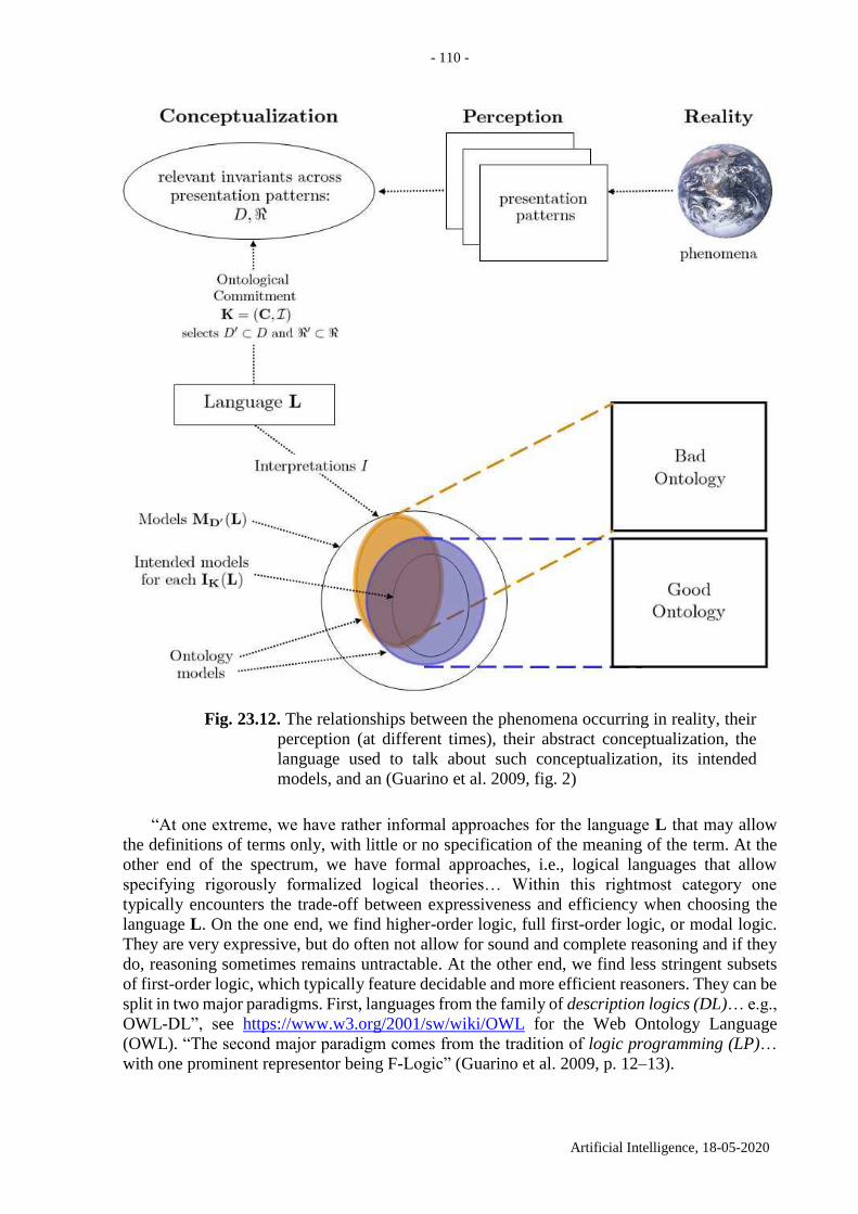
- 110 -
Artificial Intelligence, 18-05-2020
Fig. 23.12. The relationships between the phenomena occurring in reality, their
perception (at different times), their abstract conceptualization, the
language used to talk about such conceptualization, its intended
models, and an (Guarino et al. 2009, fig. 2)
“At one extreme, we have rather informal approaches for the language L that may allow
the definitions of terms only, with little or no specification of the meaning of the term. At the
other end of the spectrum, we have formal approaches, i.e., logical languages that allow
specifying rigorously formalized logical theories… Within this rightmost category one
typically encounters the trade-off between expressiveness and efficiency when choosing the
language L. On the one end, we find higher-order logic, full first-order logic, or modal logic.
They are very expressive, but do often not allow for sound and complete reasoning and if they
do, reasoning sometimes remains untractable. At the other end, we find less stringent subsets
of first-order logic, which typically feature decidable and more efficient reasoners. They can be
split in two major paradigms. First, languages from the family of description logics (DL)… e.g.,
OWL-DL”, see https://www.w3.org/2001/sw/wiki/OWL for the Web Ontology Language
(OWL). “The second major paradigm comes from the tradition of logic programming (LP)…
with one prominent representor being F-Logic” (Guarino et al. 2009, p. 12–13).
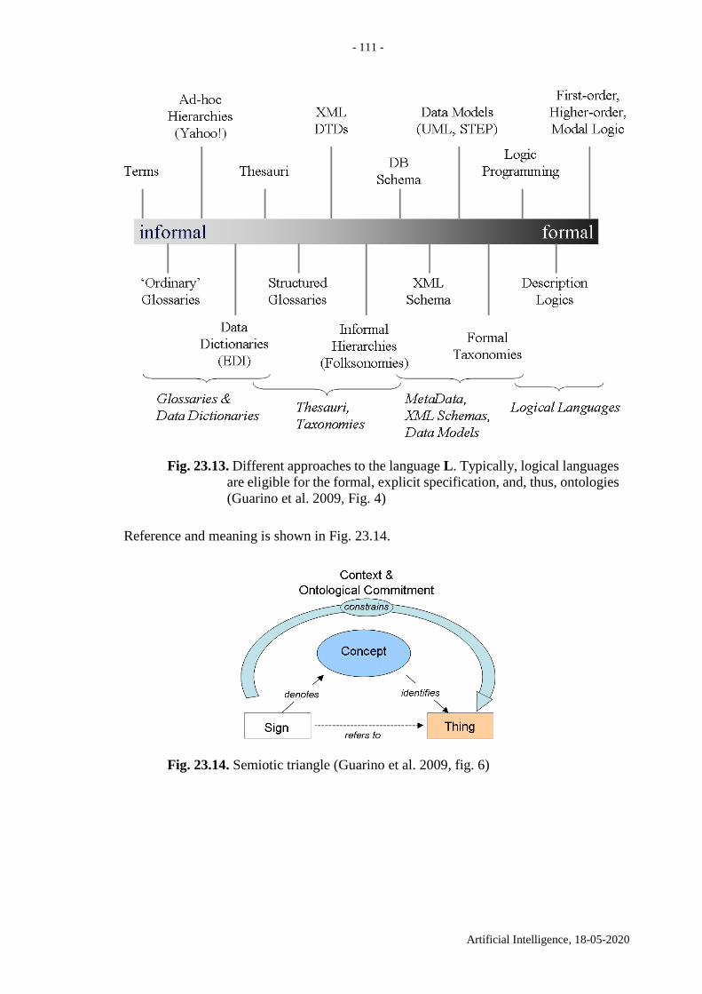
- 111 -
Artificial Intelligence, 18-05-2020
Fig. 23.13. Different approaches to the language L. Typically, logical languages
are eligible for the formal, explicit specification, and, thus, ontologies
(Guarino et al. 2009, Fig. 4)
Reference and meaning is shown in Fig. 23.14.
Fig. 23.14. Semiotic triangle (Guarino et al. 2009, fig. 6)
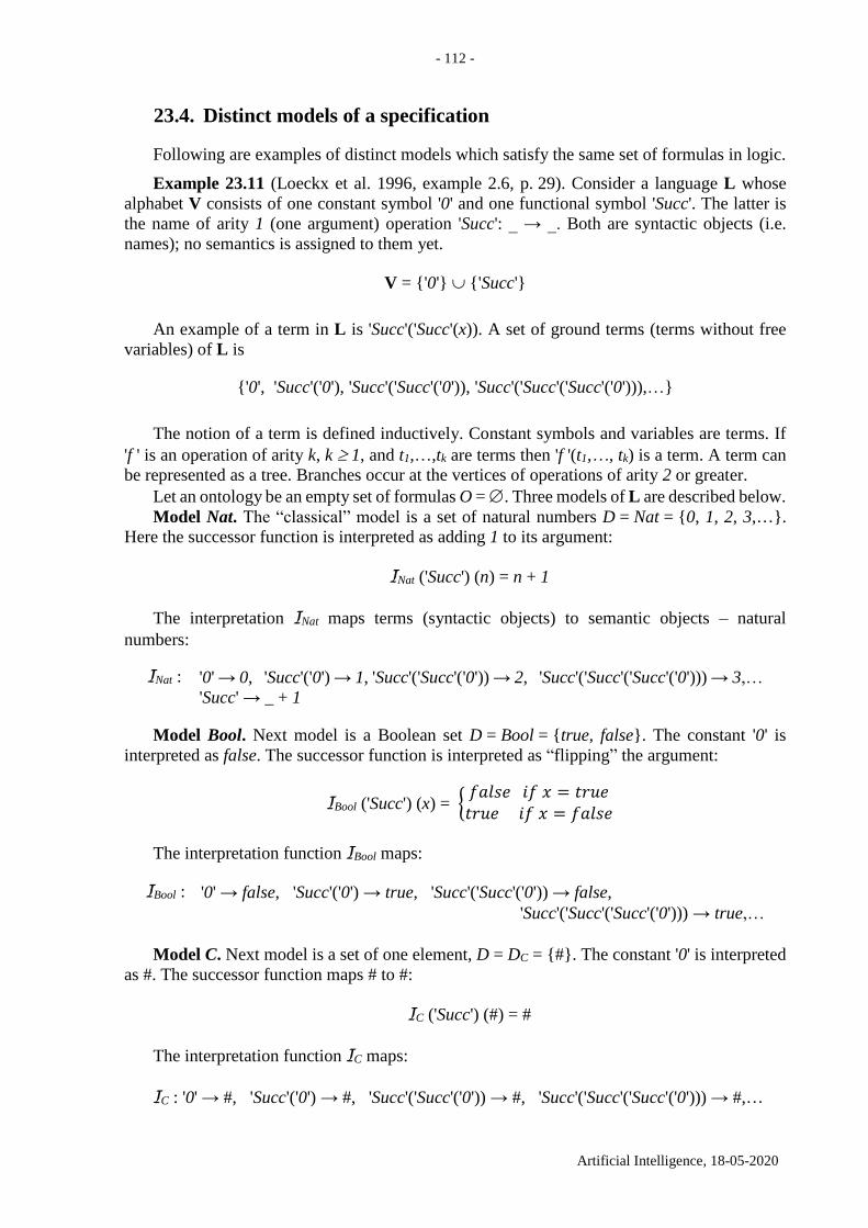
- 112 -
Artificial Intelligence, 18-05-2020
23.4. Distinct models of a specification
Following are examples of distinct models which satisfy the same set of formulas in logic.
Example 23.11 (Loeckx et al. 1996, example 2.6, p. 29). Consider a language L whose
alphabet V consists of one constant symbol '0' and one functional symbol 'Succ'. The latter is
the name of arity 1 (one argument) operation 'Succ': _ → _. Both are syntactic objects (i.e.
names); no semantics is assigned to them yet.
V = {'0'} {'Succ'}
An example of a term in L is 'Succ'('Succ'(x)). A set of ground terms (terms without free
variables) of L is
{'0', 'Succ'('0'), 'Succ'('Succ'('0')), 'Succ'('Succ'('Succ'('0'))),…}
The notion of a term is defined inductively. Constant symbols and variables are terms. If
'f ' is an operation of arity k, k 1, and t1,…,tk are terms then 'f '(t1,…, tk) is a term. A term can
be represented as a tree. Branches occur at the vertices of operations of arity 2 or greater.
Let an ontology be an empty set of formulas O =. Three models of L are described below.
Model Nat. The “classical” model is a set of natural numbers D = Nat = {0, 1, 2, 3,…}.
Here the successor function is interpreted as adding 1 to its argument:
INat ('Succ') (n) = n + 1
The interpretation INat maps terms (syntactic objects) to semantic objects – natural
numbers:
INat : '0' → 0, 'Succ'('0') → 1, 'Succ'('Succ'('0')) → 2, 'Succ'('Succ'('Succ'('0'))) → 3,…
'Succ' → _ + 1
Model Bool. Next model is a Boolean set D = Bool = {true, false}. The constant '0' is
interpreted as false. The successor function is interpreted as “flipping” the argument:
IBool ('Succ') (x) = {𝑓𝑎𝑙𝑠𝑒 𝑖𝑓 𝑥 = 𝑡𝑟𝑢𝑒𝑡𝑟𝑢𝑒 𝑖𝑓 𝑥 = 𝑓𝑎𝑙𝑠𝑒
The interpretation function IBool maps:
IBool : '0' → false, 'Succ'('0') → true, 'Succ'('Succ'('0')) → false,
'Succ'('Succ'('Succ'('0'))) → true,…
Model C. Next model is a set of one element, D = DC = {#}. The constant '0' is interpreted
as #. The successor function maps # to #:
IC ('Succ') (#) = #
The interpretation function IC maps:
IC : '0' → #, 'Succ'('0') → #, 'Succ'('Succ'('0')) → #, 'Succ'('Succ'('Succ'('0'))) → #,…
- 113 -
Artificial Intelligence, 18-05-2020
Example 23.12 (Loeckx et al. 1996, example 5.24 iv, p. 87). ). Consider a language L
whose alphabet V consists of one constant symbol '0' and one functional symbol '+':
V = {'0'} {'+'}
Let an ontology O consist of four formulas:
O = {
}
x '+' (y '+' z) = (x '+' y) '+' z,
x '+' '0' = x,
'0' '+' x = x,
x y ( x '+' y = '0' y '+' x = '0' ) }
(23.1)
The first formula expresses a property known as associativity. The second and third formula
are about the neutral element '0' for addition operation '+'. The forth formula is about the inverse
element y. All formulas in an ontology serve as axioms that specify a model.
Any group (an algebraic structure in abstract algebra) is a model for the ontology (23.1).
Below we distinguish between infinite groups and finite groups.
Model Z. The “classical” model is a set of integer numbers D = Z = {…, –3, –2, –1, 0, 1,
2, 3,…}. Here the addition operation '+' is interpreted as addition of integers:
IZ ('+' ) (n,m) = n + m
The existence of the inverse element y in the fourth formula in (23.1) can be replaced with
a Skolem term operation 'Inv'(x). This replacement is called Skolemization. The interpretation
IZ maps 'Inv' terms to invocations of an arity 1 function minus (and denoted –) for integers:
IZ ('Inv' ) (n) = –n
Integer numbers satisfy all four formulas in the ontology O (23.1) above. For all x, y Z it
is true that x + (y +z) = (x + y) + z, x + 0 = x, 0 + x = x, and the inverse element of x is –x, where
– ( –x) = x.
Model Zn. A model is set of integers D = Zn = {0, 1, 2,…, n–1}. They form a finite group
called remainder group. Here the addition operation '+' is interpreted as addition modulo n:
IZn ('+') (l,m) = l + m modulo n (or simply l n m)
In the case n=3 we have Z3 = {0, 1, 2} and
0 + 0 modulo 3 = 0 (or 0 3 0= 0)
0 + 1 modulo 3 = 1 (or 0 3 1= 1)
0 + 2 modulo 3 =2 (or 0 3 2= 2)
1 + 2 modulo 3 =0 (or 1 3 2= 0)
2 + 2 modulo 3 =1 (or 2 3 2= 1)
In the case n=2 we have Z2 = {0, 1} and write 0 0= 0, 0 1= 1, 1 1= 0.
In modular arithmetic, two integers are added and then the sum is divided by a positive
integer called the modulus. The result of modular addition is the remainder of that division. For
any modulus, n, the set of integers from 0 to n − 1 forms a group under modular addition: the
inverse of any element a is n − a, and 0 is the identity element. This is familiar from the addition
- 114 -
Artificial Intelligence, 18-05-2020
of hours on the face of a clock: if the hour hand is on 9 and is advanced 4 hours, it ends up on
1. This is expressed by saying that 9 + 4 equals 1 “modulo 12” or, in symbols, 9 + 4 ≡ 1 modulo
12. The group of integers modulo n is written Zn; see
https://en.wikipedia.org/wiki/Group_(mathematics).
Example 23.13 (Loeckx et al. 1996, example 5.24 iv, p. 87). Consider a language L whose
alphabet V consists of one constant symbol '0' and two functional symbols, '+' and 'Succ':
V = {'0'} {'+', 'Succ'}
Let an ontology consist of two formulas:
O = { x '+' '0' = x,
'Succ'(x '+' y) = x '+' 'Succ'(y)} (23.2)
The first formula is about the neutral element '0' for addition operation '+'. The second formula
is about a flowdown of 'Succ'.
A model is constituted by natural numbers D = {0, 1, 2, 3,…}. Here the successor function
is interpreted as adding 1 to its argument. Arithmetical addition, +, is the second function on D.
The interpretation function I maps:
I : '0' → 0, 'Succ'('0') → 1, 'Succ'('Succ'('0')) → 2, 'Succ'('Succ'('Succ'('0'))) → 3,…
'+' → +,
'Succ' → _ + 1
The meaning of the last line, 'Succ' → _ + 1, is as follows. The functional symbol 'Succ' is
mapped to arity 1 (one argument) function which adds 1 to its argument. Natural numbers
satisfy both formulae in the ontology O (23.2): for all x, y D it is true that x + 0 = x and
(x + y) + 1 = x + (y +1).
Next model is constituted by even numbers, D = {0, 2, 4, 6,…}. Here the successor
operation 'Succ' is interpreted as adding 2 to its argument. The interpretation function I maps:
I : '0' → 0, 'Succ'('0') → 2, 'Succ'('Succ'('0')) → 4, 'Succ'('Succ'('Succ'('0'))) → 6,…
'+' → +,
'Succ' → _ + 2
The last line above, 'Succ' → _ + 2, means that the functional symbol 'Succ' is mapped to arity
1 function which adds 2 to its argument. The set of even numbers is isomorphic to the set of
natural numbers. Therefore even numbers are not considered as a model.
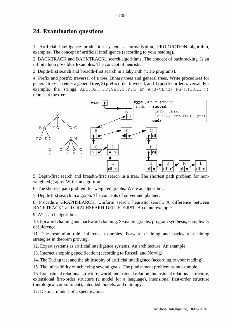
- 115 -
Artificial Intelligence, 18-05-2020
24. Examination questions
1. Artificial intelligence production system, a formalisation, PRODUCTION algorithm,
examples. The concept of artificial intelligence (according to your reading).
2. BACKTRACK and BACKTRACK1 search algorithms. The concept of backtracking. Is an
infinite loop possible? Examples. The concept of heuristic.
3. Depth-first search and breadth-first search in a labyrinth (write programs).
4. Prefix and postfix traversal of a tree. Binary trees and general trees. Write procedures for
general trees: 1) enter a general tree, 2) prefix order traversal, and 3) postfix order traversal. For
example, the strings ABC.DE...F.GHI.J.K.L or A(B(CD(E))FG(H(IJKL)))
represent the tree:
5. Depth-first search and breadth-first search in a tree. The shortest path problem for non-
weighted graphs. Write an algorithm.
6. The shortest path problem for weighted graphs. Write an algorithm.
7. Depth-first search in a graph. The concepts of solver and planner.
8. Procedure GRAPHSEARCH. Uniform search, heuristic search. A difference between
BACKTRACK1 and GRAPHSEARH-DEPTH-FIRST. A counterexample.
9. A* search algorithm.
10. Forward chaining and backward chaining. Semantic graphs, program synthesis, complexity
of inference.
11. The resolution rule. Inference examples. Forward chaining and backward chaining
strategies in theorem proving.
12. Expert systems as artificial intelligence systems. An architecture. An example.
13. Internet shopping specification (according to Russell and Norvig).
14. The Turing test and the philosophy of artificial intelligence (according to your reading).
15. The infeasibility of achieving several goals. The punishment problem as an example.
16. Extensional relational structure, world, intensional relation, intensional relational structure,
extensional first-order structure (a model for a language), intensional first-order structure
(ontological commitment), intended models, and ontology.
17. Distinct models of a specification.
- 116 -
Artificial Intelligence, 18-05-2020
25. References
Main list
1. Luger, George (2009) Artificial intelligence: structures and strategies for complex problem
solving (6th ed.). Addison-Wesley. http://www.cs.unm.edu/~luger/. VU MIF: 004.8/Lu-59.
2. Michael Negnevitsky (2011) Artificial intelligence: a guide to intelligent systems (3rd ed.).
Addison-Wesley, 2011. VU MIF: 004.8/Ne-44.
3. Russell, Stuart; Norvig, Peter (2010) Artificial intelligence: a modern approach (3rd ed.).
Prentice Hall. http://aima.cs.berkeley.edu. VU MIF: 004.8/Ru-151.
Supplementary list
4. Antoniou, G.; Groth, P.; van Harmelen, F.; Hoekstra, R. (2012) A semantic web primer (3rd
ed.). The MIT Press. VU MIF 004.8/An-154.
5. Nilsson, Nils (2010) The quest for artificial intelligence: a history of ideas and
achievements. Cambridge University Press. VU MIF: 004.8/Ni-133.
6. Nilsson, Nils (1998) Artificial intelligence: a new synthesis. Morgan Kaufmann Publishers.
VU MIF: 004.8/Ni-133.
7. Nilsson, Nils (1982) Principles of artificial intelligence. Springer, Berlin Heidelberg.
8. Sowa, John F. (2000) Knowledge representation: logical philosophical, and computational
foundations. Brooks/Cole, Pacific Grove.
Other references
9. Bench-Capon, T. J. M.; Prakken, H. (2006) Justifying actions by accruing arguments. In:
Computational Models of Argument – Proceedings of COMMA 2006, IOS Press, pp. 247–
258. IOS Press. http://www.cs.uu.nl/groups/IS/archive/henry/action.pdf, slides
http://www.cs.uu.nl/deon2006/tbc+hp.pdf.
10. E. D. Falkenberg, W. Hesse, P. Lindgreen, B. E. Nilsson, J. L. H. Oei, C. Rolland, R. K.
Stamper, F. J. M. Van Assche, A. A. Verrijn-Stuart, K. Voss (1998) A framework of
information system concepts, The FRISCO Report (Web edition), IFIP, the Netherlands.
http://www.mathematik.uni-marburg.de/~hesse/papers/fri-full.pdf.
11. Guarino, N.; Oberle, D.; Staab, S. (2009) What is an Ontology? In: Handbook on
Ontologies, S. Staab, R. Studer (eds.) pp. 1–17, Springer.
http://iaoa.org/isc2012/docs/Guarino2009_What_is_an_Ontology.pdf.
12. Hesse, W.; A. Verrijn-Stuart, A. (2001) Towards a theory of information systems: the
FRISCO approach. In: H. Jaakkola et al. (eds.) Information Modelling and Knowledge
Bases XII, p. 81–91. IOS Press, Amsterdam.
13. Loeckx, Jacques; Ehrich, Hans-Dieter; Wolf, Markus (1996) Specification of abstract data
types. Wiley-Teubner, Chichester.
14. McCarthy, John (2007) What is artificial intelligence? http://www-
formal.stanford.edu/jmc/whatisai.pdf.
15. Sawyer, Brian; Foster, Dennis (1986) Programming expert systems in Pascal. John Wiley,
New York.
16. Thayse, Andre; Gribomont, Pascal; Louis, Georges et al. (1988) Approche logique de
l'intelligence artificielle. Dunot, Paris.
17. Turing, Alan M. (1950) Computing machinery and intelligence. Mind, 1950, vol. 59.
no. 236, pp. 433–460. http://mind.oxfordjournals.org/content/LIX/236/433.