artificial neural network
TRANSCRIPT
An Introduction to Artificial Neural
Network
Dr Iman Ardekani
Iman Ardekani
Biological Neurons
Modeling Neurons
McCulloch-Pitts Neuron
Network Architecture
Learning Process
Perceptron
Linear Neuron
Multilayer Perceptron
Content
Iman Ardekani
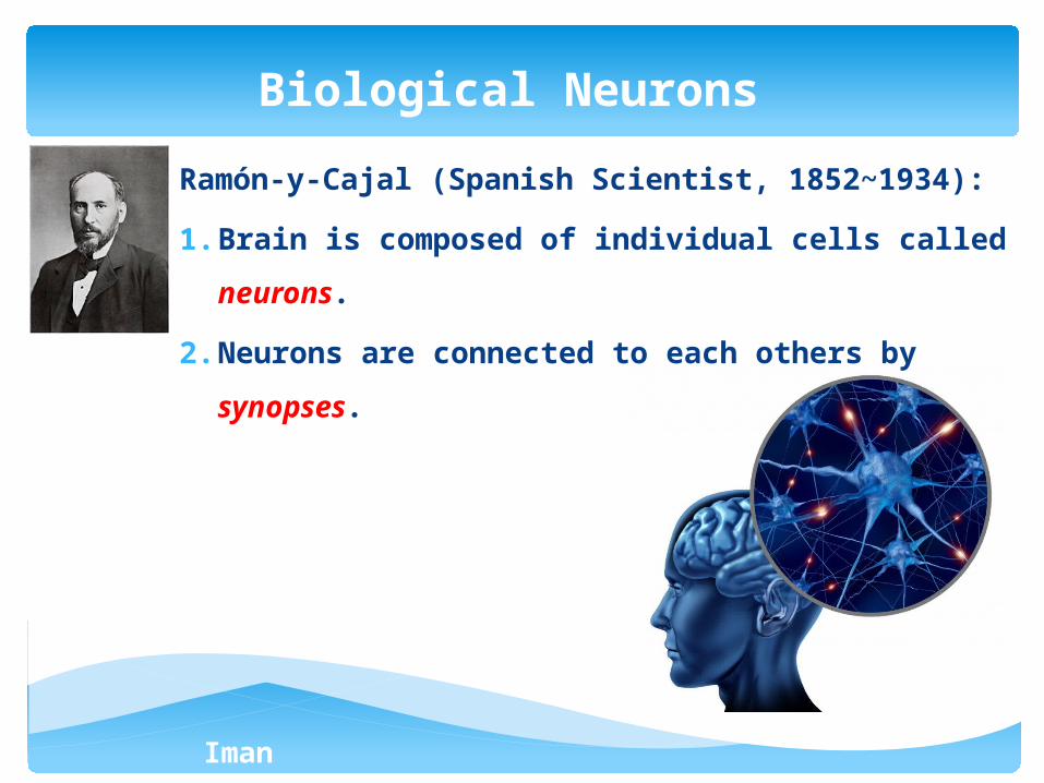
Ramón-y-Cajal (Spanish Scientist, 1852~1934):
1. Brain is composed of individual cells called
neurons.
2. Neurons are connected to each others by
synopses.
Biological Neurons
Iman Ardekani
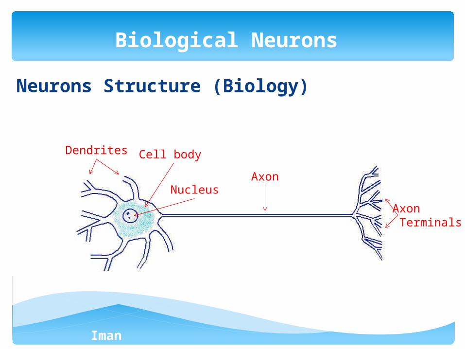
Neurons Structure (Biology)
Biological Neurons
Dendrites Cell body
NucleusAxon
Axon Terminals
Iman Ardekani
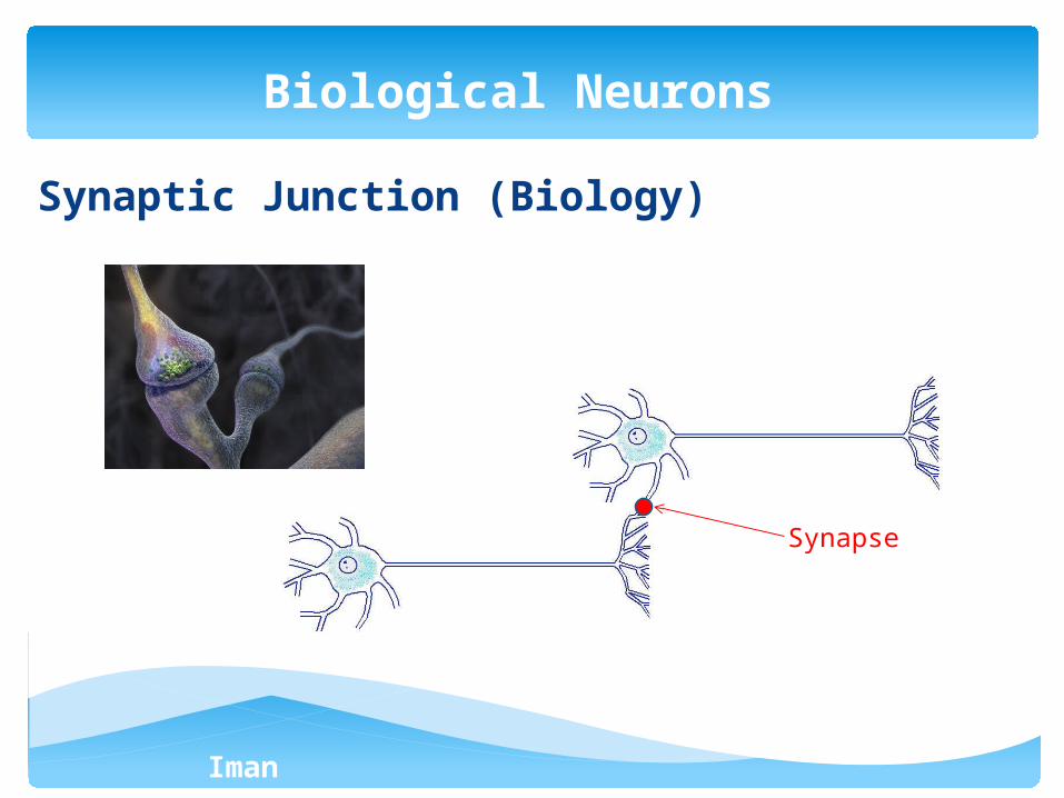
Synaptic Junction (Biology)
Biological Neurons
Synapse
Iman Ardekani
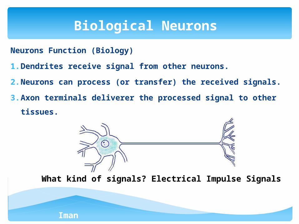
Neurons Function (Biology)
1. Dendrites receive signal from other neurons.
2. Neurons can process (or transfer) the received signals.
3. Axon terminals deliverer the processed signal to other
tissues.
Biological Neurons
What kind of signals? Electrical Impulse Signals
Iman Ardekani
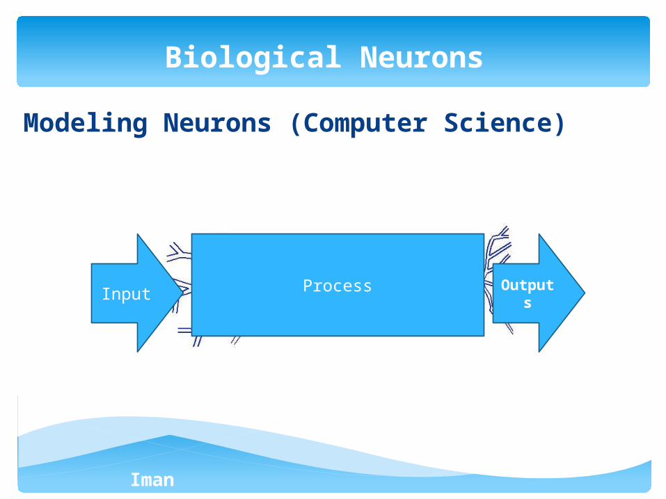
Modeling Neurons (Computer Science)
Biological Neurons
Input Outputs
Process
Iman Ardekani
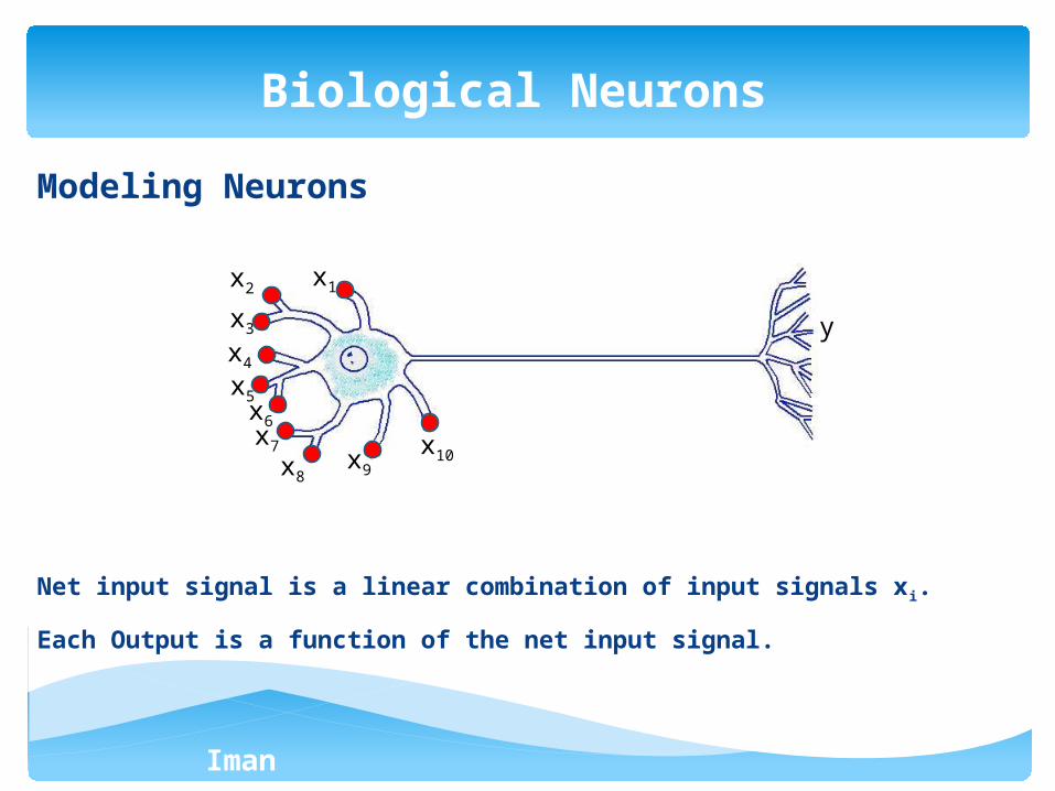
Modeling Neurons
Net input signal is a linear combination of input signals xi.
Each Output is a function of the net input signal.
Biological Neurons
x1x2
x3
x4
x5x6x7
x8x9
x10
y
Iman Ardekani
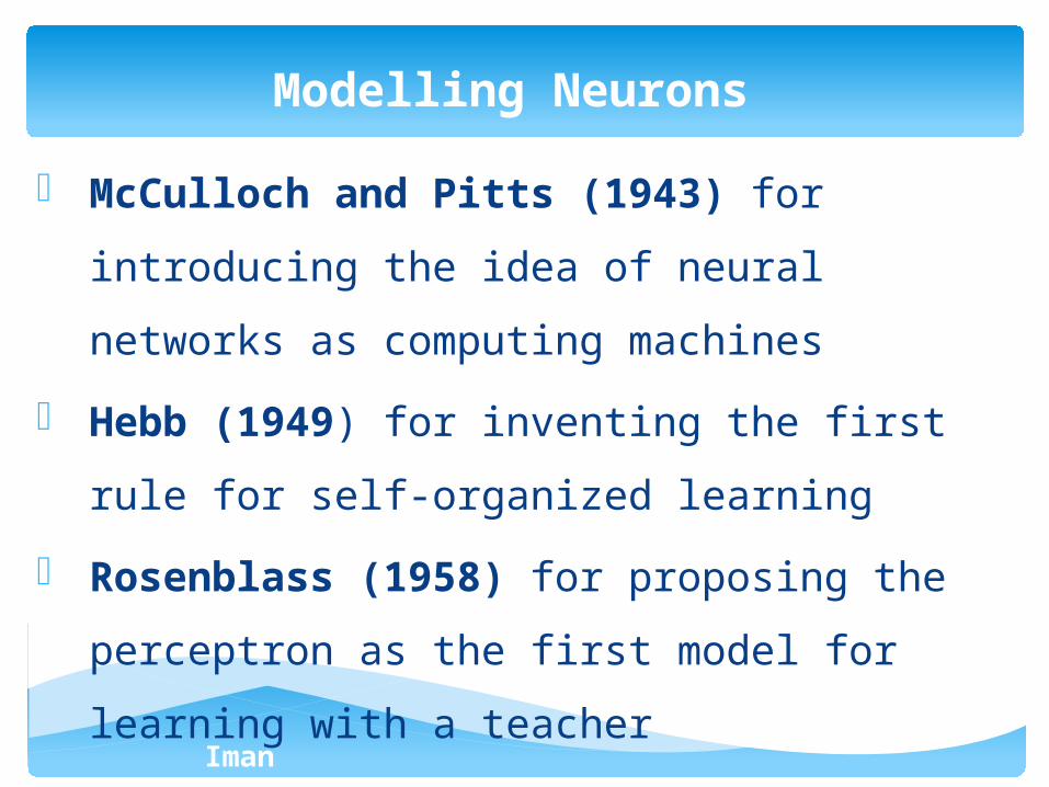
- McCulloch and Pitts (1943) for introducing the
idea of neural networks as computing machines
- Hebb (1949) for inventing the first rule for self-
organized learning
- Rosenblass (1958) for proposing the perceptron
as the first model for learning with a teacher
Modelling Neurons
Iman Ardekani
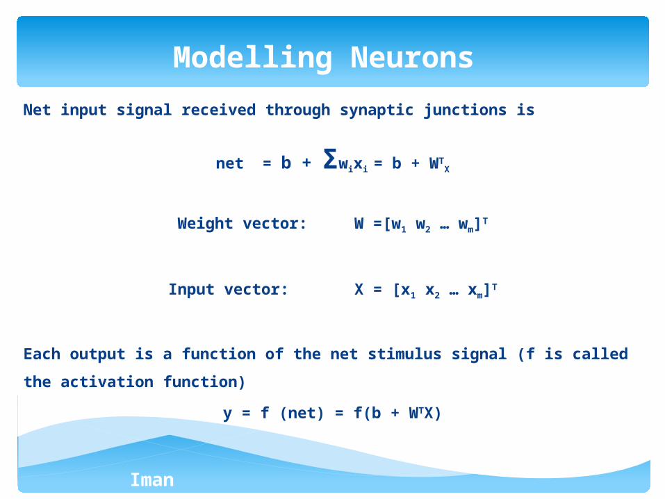
Net input signal received through synaptic junctions is
net = b + Σwixi = b + WTX
Weight vector: W =[w1 w2 … wm]T
Input vector: X = [x1 x2 … xm]T
Each output is a function of the net stimulus signal (f is called the activation
function)
y = f (net) = f(b + WTX)
Modelling Neurons
Iman Ardekani
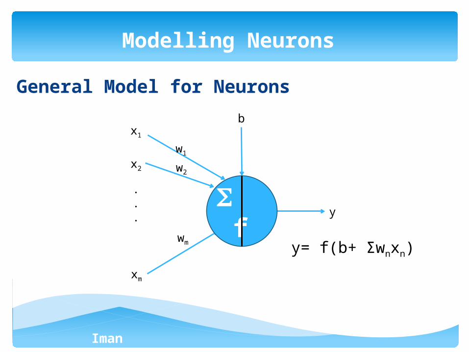
General Model for Neurons
Modelling Neurons
y= f(b+ Σwnxn)
x1
x2
xm
.
.
. y
w1
w2
wm
b
f
Iman Ardekani
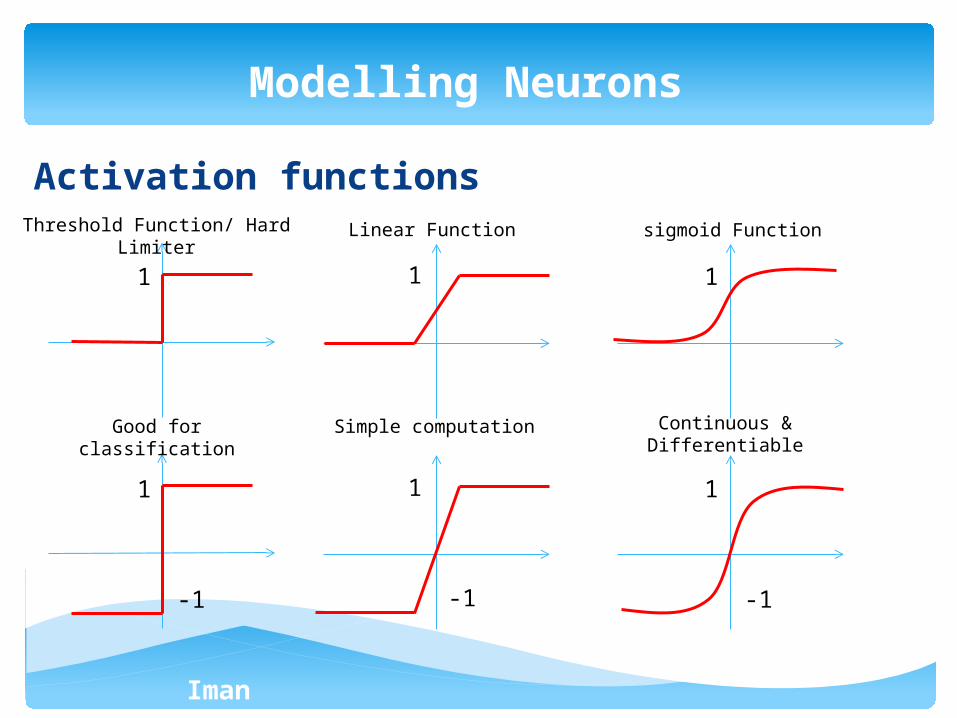
Activation functions
Modelling Neurons
1 1 1
1 1 1
-1 -1 -1
Good for classification
Simple computation Continuous & Differentiable
Threshold Function/ Hard Limiter
Linear Function sigmoid Function
Iman Ardekani
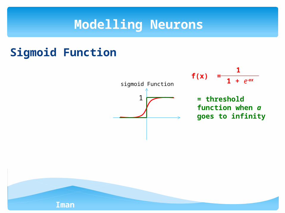
Sigmoid Function
Modelling Neurons
1
sigmoid Functionf(x) =
1
1 + e-ax
= threshold function when a goes to infinity
Iman Ardekani
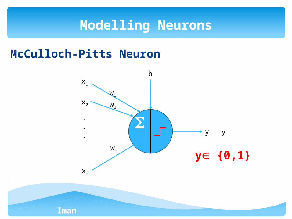
McCulloch-Pitts Neuron
Modelling Neurons
y {0,1}
y
x1
x2
xm
.
.
. y
w1
w2
wm
b
Iman Ardekani
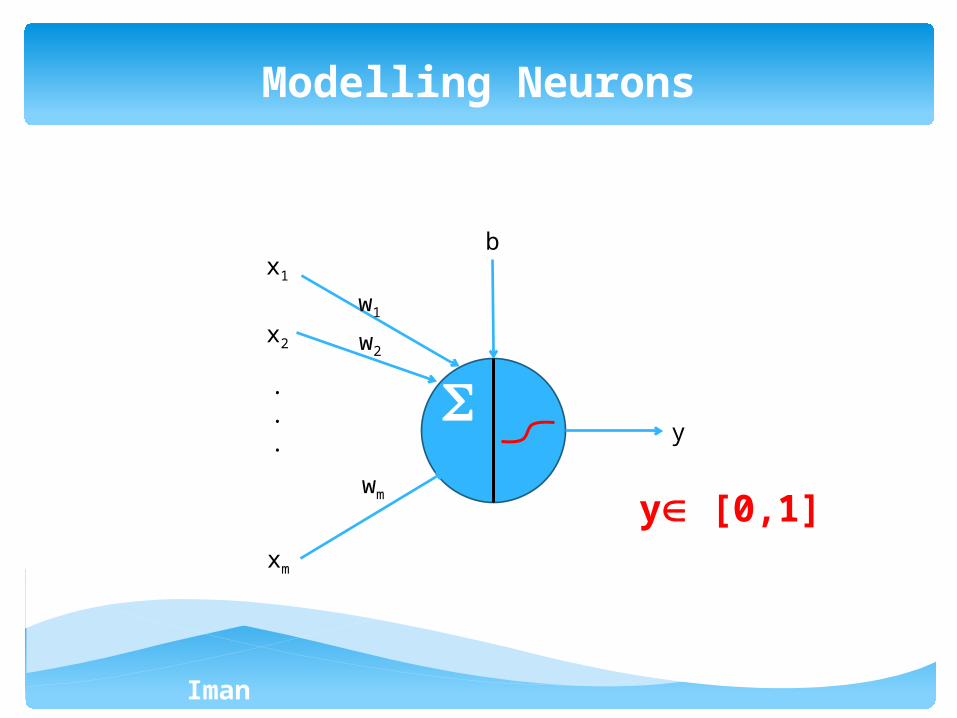
Modelling Neurons
y [0,1]
x1
x2
xm
.
.
. y
w1
w2
wm
b
Iman Ardekani
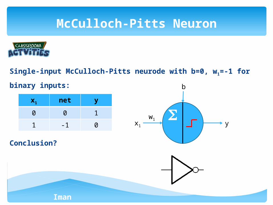
Single-input McCulloch-Pitts neurode with b=0, w1=-1 for binary inputs:
Conclusion?
McCulloch-Pitts Neuron
x1 net y
0 0 1
1 -1 0 x1 yw1
b
Iman Ardekani
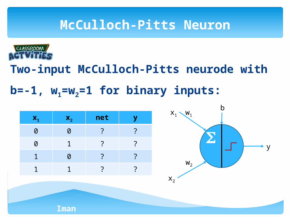
Two-input McCulloch-Pitts neurode with b=-1,
w1=w2=1 for binary inputs:
McCulloch-Pitts Neuron
x1 x2 net y
0 0 ? ?
0 1 ? ?
1 0 ? ?
1 1 ? ?
x1
y
w1
b
x2
w2
Iman Ardekani
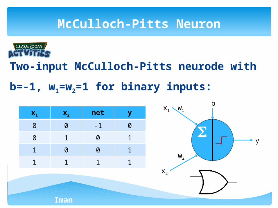
Two-input McCulloch-Pitts neurode with b=-1,
w1=w2=1 for binary inputs:
McCulloch-Pitts Neuron
x1 x2 net y
0 0 -1 0
0 1 0 1
1 0 0 1
1 1 1 1
x1
y
w1
b
x2
w2

Iman Ardekani
Two-input McCulloch-Pitts neurode with b=-2,
w1=w2=1 for binary inputs :
McCulloch-Pitts Neuron
x1 x2 net y
0 0 ? ?
0 1 ? ?
1 0 ? ?
1 1 ? ?
x1
y
w1
b
x2
w2

Iman Ardekani
Two-input McCulloch-Pitts neurode with b=-2,
w1=w2=1 for binary inputs :
McCulloch-Pitts Neuron
x1 x2 net y
0 0 -2 0
0 1 -1 0
1 0 -1 0
1 1 0 1
x1
y
w1
b
x2
w2
Iman Ardekani
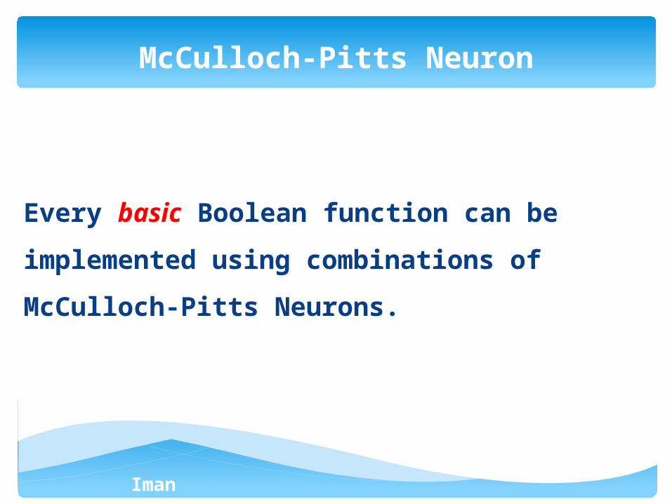
Every basic Boolean function can be implemented
using combinations of McCulloch-Pitts Neurons.
McCulloch-Pitts Neuron
Iman Ardekani
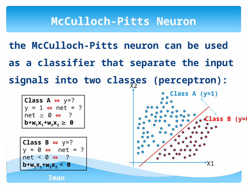
the McCulloch-Pitts neuron can be used as a
classifier that separate the input signals into two
classes (perceptron):
McCulloch-Pitts Neuron
X1
X2 Class A (y=1)
Class B (y=0)
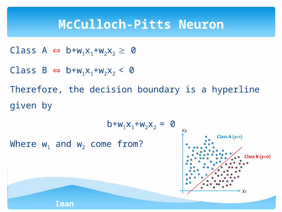
Class A y=?y = 1 net = ?net 0 ?b+w1x1+w2x2 0
Class B y=?y = 0 net = ?net < 0 ?b+w1x1+w2x2 < 0
Iman Ardekani
Class A b+w1x1+w2x2 0
Class B b+w1x1+w2x2 < 0
Therefore, the decision boundary is a hyperline given by
b+w1x1+w2x2 = 0
Where w1 and w2 come from?
McCulloch-Pitts Neuron
Iman Ardekani
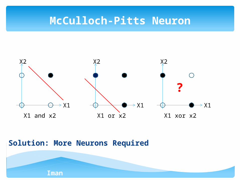
Solution: More Neurons Required
McCulloch-Pitts Neuron
X2
X1
X1 and x2
X2
X1
X1 or x2
X2
X1
X1 xor x2
?
Iman Ardekani
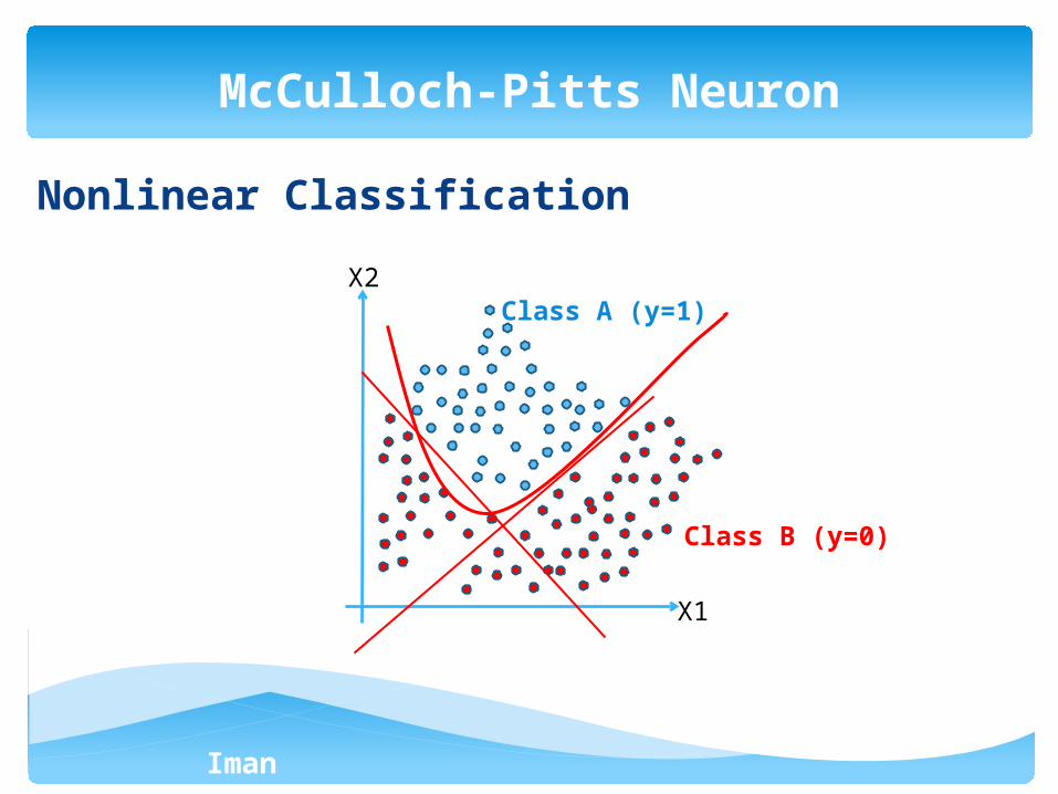
Nonlinear Classification
McCulloch-Pitts Neuron
X1
X2 Class A (y=1)
Class B (y=0)
Iman Ardekani
Single Layer Feed-forward Network
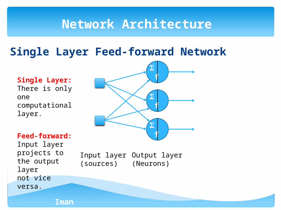
Network Architecture
Single Layer:There is only one computational layer.
Feed-forward:Input layer projects to the output layer not vice versa.
f
f
f
Input layer (sources)
Output layer (Neurons)
Iman Ardekani
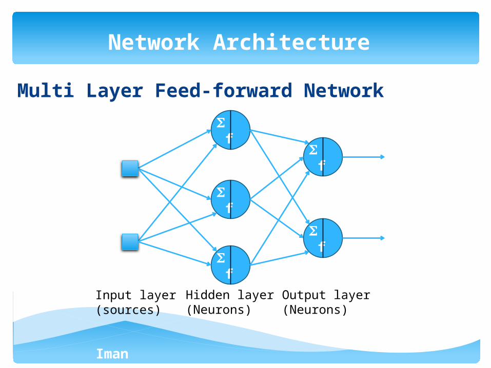
Multi Layer Feed-forward Network
Network Architecture
f
f
f
Input layer (sources)
Hidden layer (Neurons)
f
f
Output layer (Neurons)
Iman Ardekani
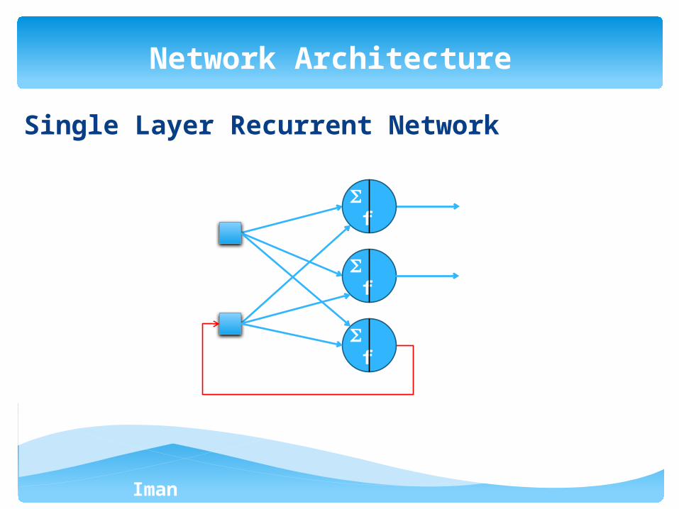
Single Layer Recurrent Network
Network Architecture
f
f
f
Iman Ardekani
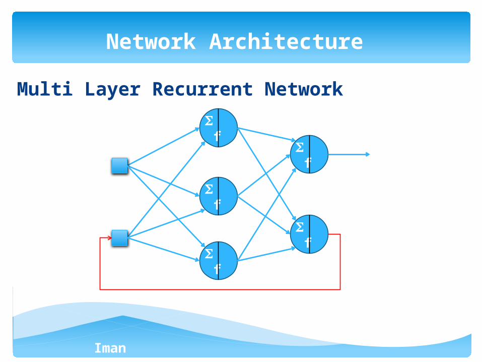
Multi Layer Recurrent Network
Network Architecture
f
f
f
f
f
Iman Ardekani
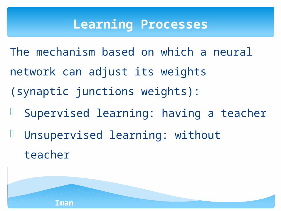
The mechanism based on which a neural network
can adjust its weights (synaptic junctions weights):
Supervised learning: having a teacher
Unsupervised learning: without teacher
Learning Processes
Iman Ardekani
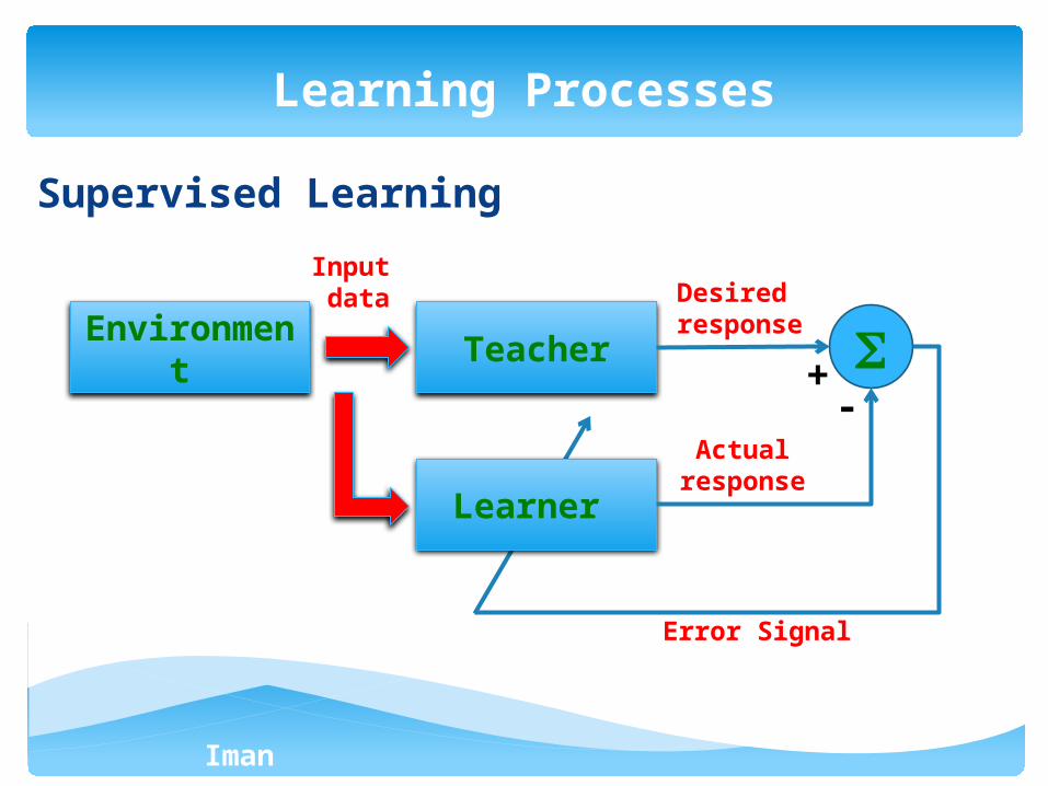
Supervised Learning
Learning Processes
Teacher
Learner
Environment
Input data Desired
response
Actualresponse
Error Signal
+-
Iman Ardekani
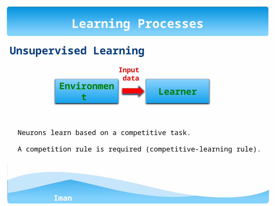
Unsupervised Learning
Learning Processes
LearnerEnvironme
nt
Input data
Neurons learn based on a competitive task.
A competition rule is required (competitive-learning rule).
Iman Ardekani
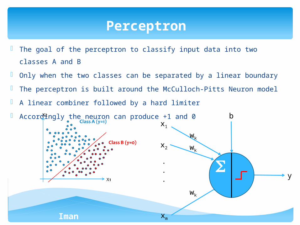
- The goal of the perceptron to classify input data into two classes A and B
- Only when the two classes can be separated by a linear boundary
- The perceptron is built around the McCulloch-Pitts Neuron model
- A linear combiner followed by a hard limiter
- Accordingly the neuron can produce +1 and 0
Perceptron
x1
x2
xm
.
.
. y
wk
wk
wk
b
Iman Ardekani
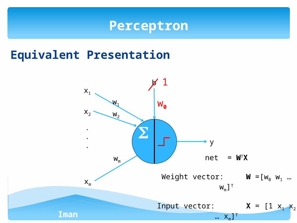
Equivalent Presentation
Perceptron
x1
x2
xm
.
.
. y
w1
w2
wm
b
w0
1
net = WTX
Weight vector: W =[w0 w1 … wm]T
Input vector: X = [1 x1 x2 … xm]T
Iman Ardekani
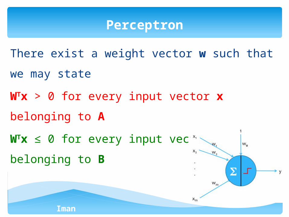
There exist a weight vector w such that we may state
WTx > 0 for every input vector x belonging to A
WTx ≤ 0 for every input vector x belonging to B
Perceptron
Iman Ardekani
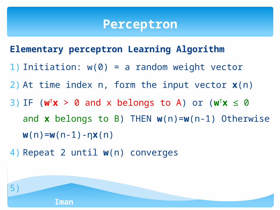
Elementary perceptron Learning Algorithm
1) Initiation: w(0) = a random weight vector
2) At time index n, form the input vector x(n)
3) IF (wTx > 0 and x belongs to A) or (wTx ≤ 0 and x belongs
to B) THEN w(n)=w(n-1) Otherwise w(n)=w(n-1)-ηx(n)
4) Repeat 2 until w(n) converges
5)
Perceptron
Iman Ardekani
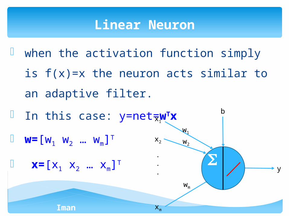
- when the activation function simply is f(x)=x the
neuron acts similar to an adaptive filter.
- In this case: y=net=wTx
- w=[w1 w2 … wm]T
- x=[x1 x2 … xm]T
Linear Neuron
x1
x2
xm
.
.
. y
w1
w2
wm
b
Iman Ardekani
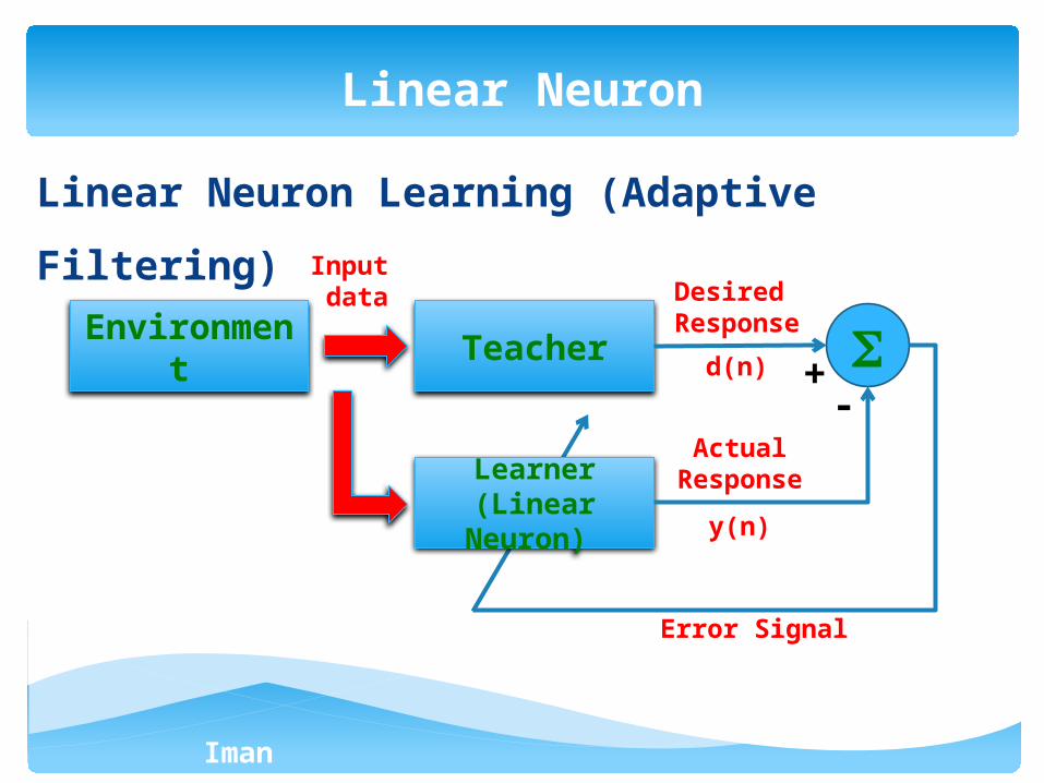
Linear Neuron Learning (Adaptive Filtering)
Linear Neuron
Teacher
Learner (Linear
Neuron)
Environment
Input data Desired
Response
d(n)
ActualResponse
y(n)
Error Signal
+-
Iman Ardekani
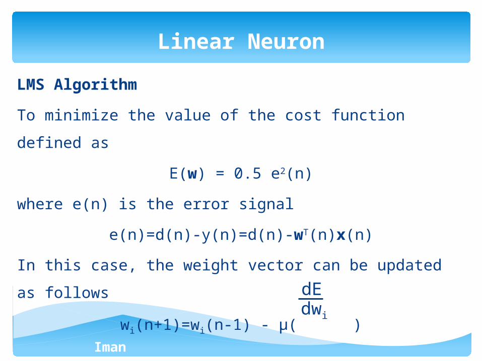
LMS Algorithm
To minimize the value of the cost function defined as
E(w) = 0.5 e2(n)
where e(n) is the error signal
e(n)=d(n)-y(n)=d(n)-wT(n)x(n)
In this case, the weight vector can be updated as follows
wi(n+1)=wi(n-1) - μ( )
Linear Neuron
dEdwi
Iman Ardekani
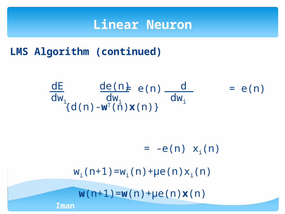
LMS Algorithm (continued)
= e(n) = e(n) {d(n)-wT(n)x(n)}
= -e(n) xi(n)
wi(n+1)=wi(n)+μe(n)xi(n)
w(n+1)=w(n)+μe(n)x(n)
Linear Neuron
dEdwi
de(n)dwi
ddwi
Iman Ardekani
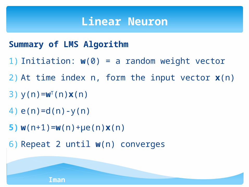
Summary of LMS Algorithm
1) Initiation: w(0) = a random weight vector
2) At time index n, form the input vector x(n)
3) y(n)=wT(n)x(n)
4) e(n)=d(n)-y(n)
5) w(n+1)=w(n)+μe(n)x(n)
6) Repeat 2 until w(n) converges
Linear Neuron
Iman Ardekani
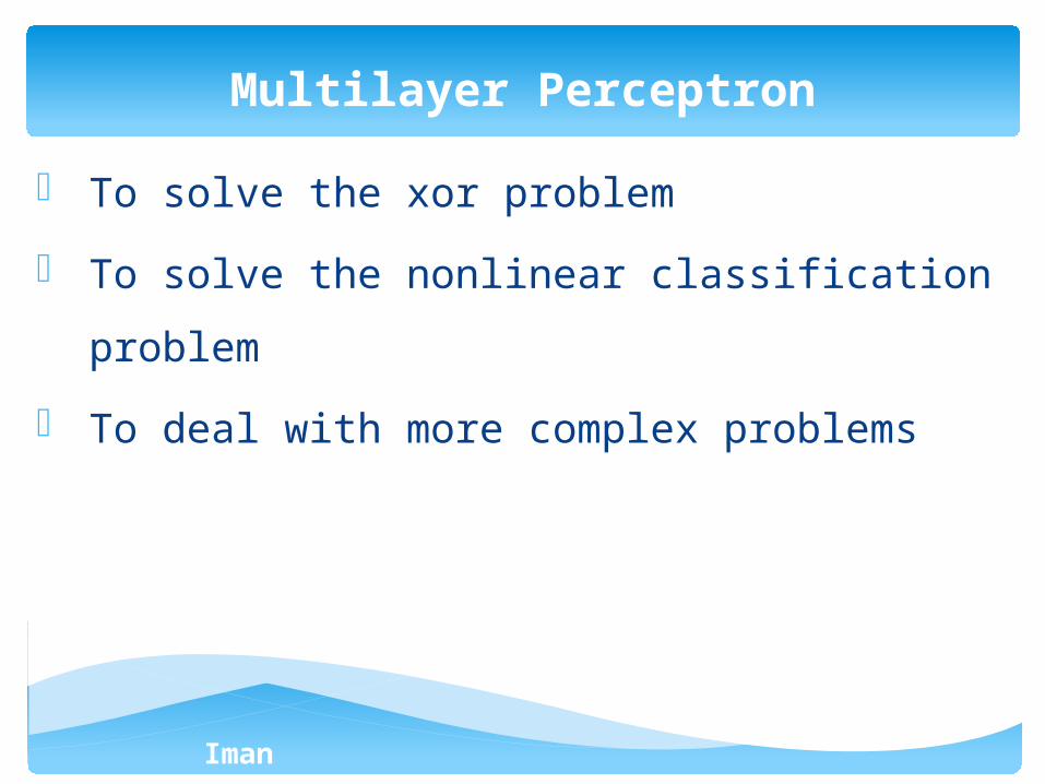
- To solve the xor problem
- To solve the nonlinear classification problem
- To deal with more complex problems
Multilayer Perceptron
Iman Ardekani
- The activation function in multilayer perceptron is
usually a Sigmoid function.
- Because Sigmoid is differentiable function, unlike
the hard limiter function used in the elementary
perceptron.
Multilayer Perceptron
Iman Ardekani
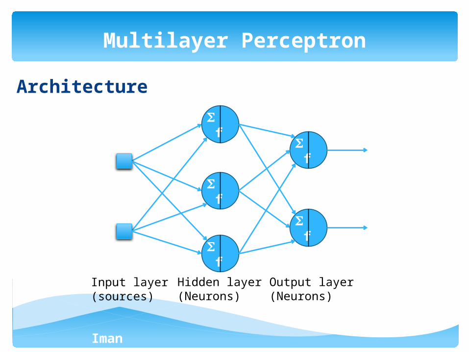
Architecture
Multilayer Perceptron
f
f
f
Input layer (sources)
Hidden layer (Neurons)
f
f
Output layer (Neurons)
Iman Ardekani
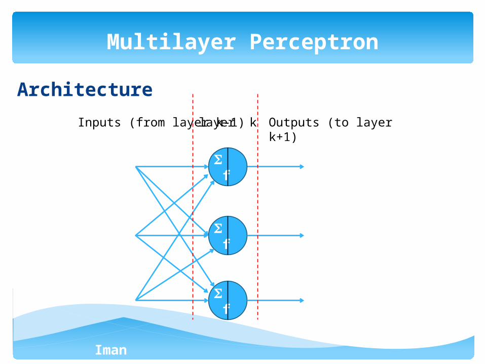
Architecture
Multilayer Perceptron
f
f
f
Inputs (from layer k-1)layer k Outputs (to layer k+1)
Iman Ardekani
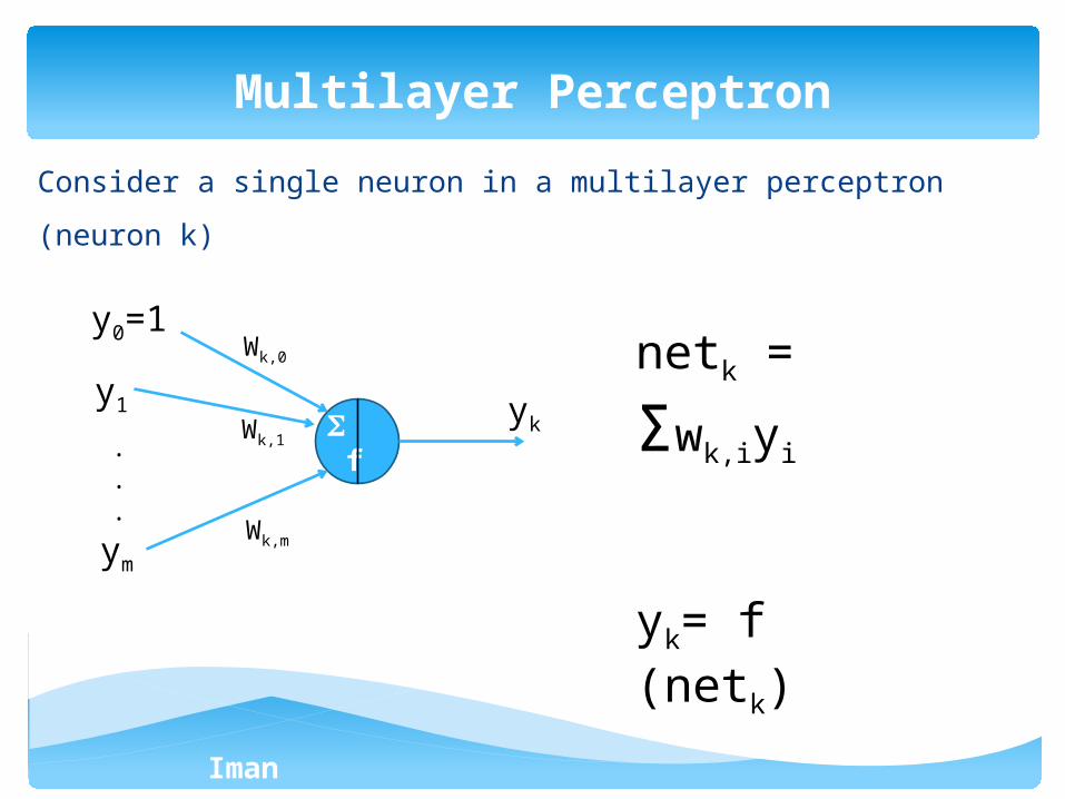
Consider a single neuron in a multilayer perceptron (neuron k)
Multilayer Perceptron
f
yk
y0=1
y1
ym
Wk,0
Wk,1
Wk,m
.
.
.
netk =
Σwk,iyi
yk= f (netk)
Iman Ardekani
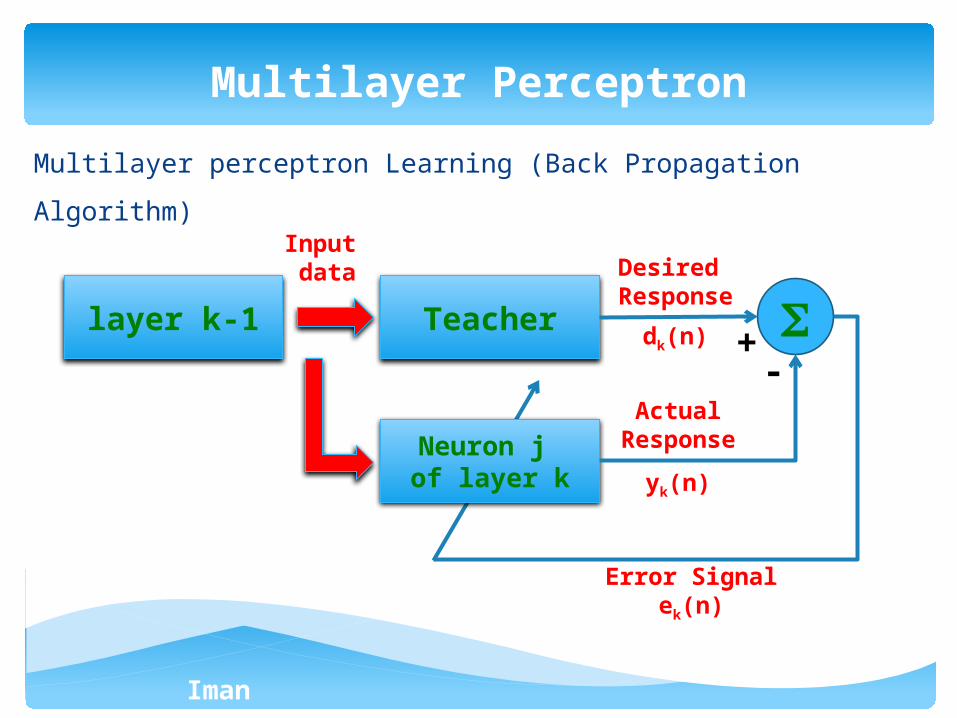
Multilayer perceptron Learning (Back Propagation Algorithm)
Multilayer Perceptron
Teacher
Neuron j of layer k
layer k-1
Input data Desired
Response
dk(n)
ActualResponse
yk(n)
Error Signalek(n)
+-
Iman Ardekani
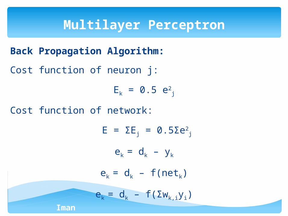
Back Propagation Algorithm:
Cost function of neuron j:
Ek = 0.5 e2j
Cost function of network:
E = ΣEj = 0.5Σe2j
ek = dk – yk
ek = dk – f(netk)
ek = dk – f(Σwk,iyi)
Multilayer Perceptron
Iman Ardekani
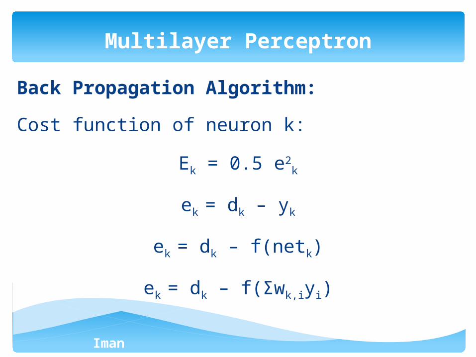
Back Propagation Algorithm:
Cost function of neuron k:
Ek = 0.5 e2k
ek = dk – yk
ek = dk – f(netk)
ek = dk – f(Σwk,iyi)
Multilayer Perceptron
Iman Ardekani
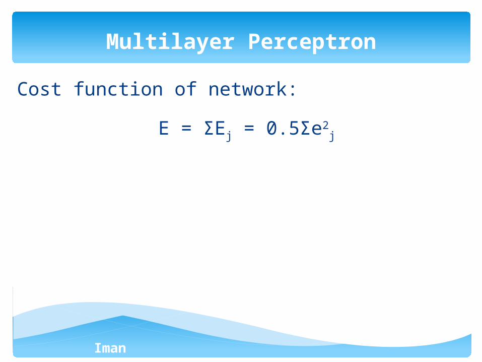
Cost function of network:
E = ΣEj = 0.5Σe2j
Multilayer Perceptron
Iman Ardekani
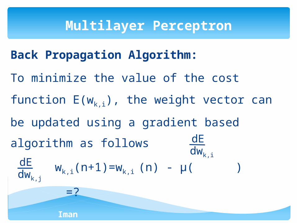
Back Propagation Algorithm:
To minimize the value of the cost function E(wk,i), the
weight vector can be updated using a gradient based
algorithm as follows
wk,i(n+1)=wk,i (n) - μ( )
=?
Multilayer Perceptron
dEdwk,i
dEdwk,j
Iman Ardekani
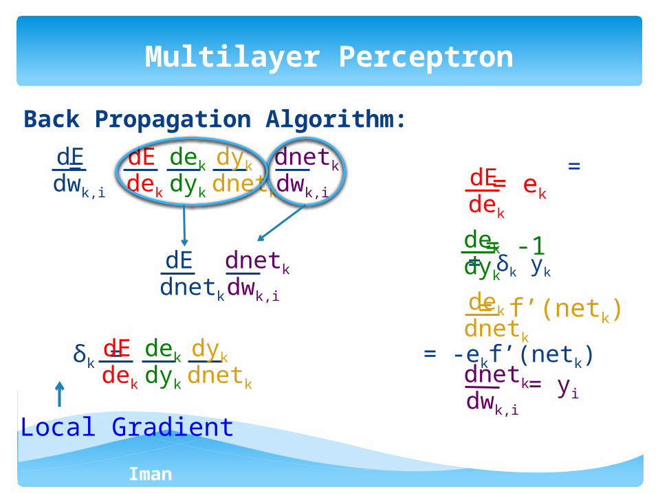
Back Propagation Algorithm:
= =
= δk yk
δk = = -ekf’(netk)
Multilayer Perceptron
dEdwk,i
dEdek
dek
dyk
dyk
dnetk
dnetk
dwk,i
dEdnetk
dnetk
dwk,i
dEdek
dek
dyk
dyk
dnetk
dEdek
= ek
dek
dnetk
= f’(netk)
dek
dyk
= -1
dnetk
dwk,i
= yi
Local Gradient
Iman Ardekani
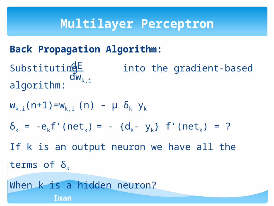
Back Propagation Algorithm:
Substituting into the gradient-based algorithm:
wk,i(n+1)=wk,i (n) – μ δk yk
δk = -ekf’(netk) = - {dk- yk} f’(netk) = ?
If k is an output neuron we have all the terms of δk
When k is a hidden neuron?
Multilayer Perceptron
dEdwk,i
Iman Ardekani
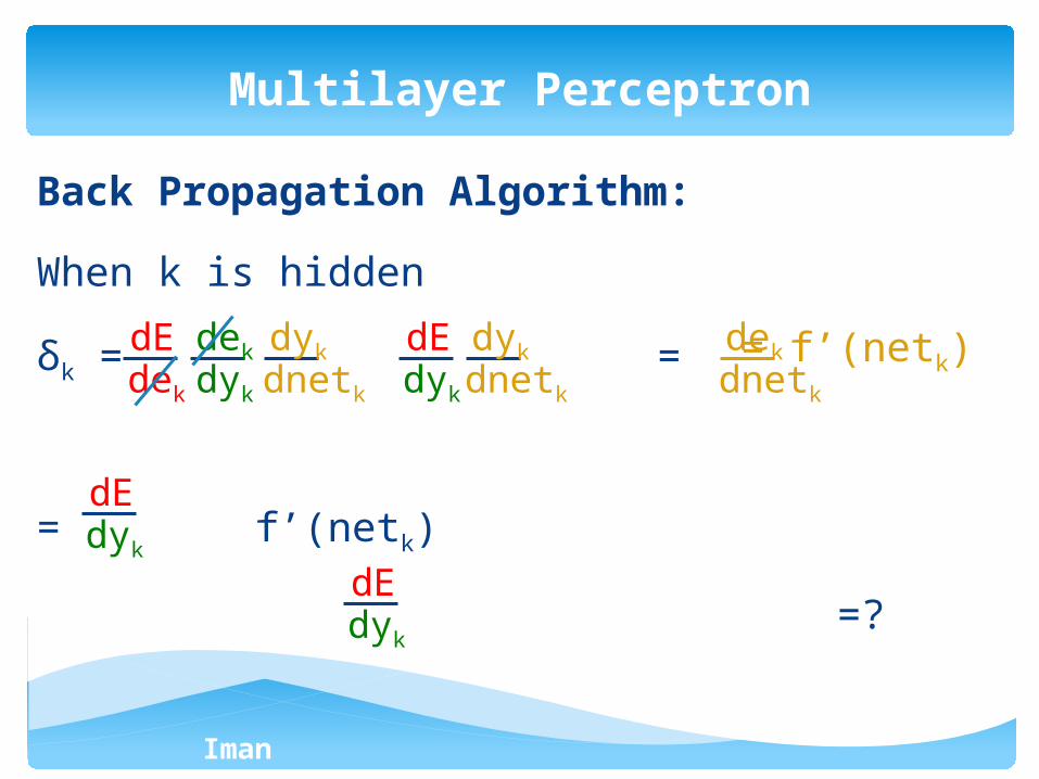
Back Propagation Algorithm:
When k is hidden
δk = =
= f’(netk)
=?
Multilayer Perceptron
dEdek
dek
dyk
dyk
dnetk
dEdyk
dyk
dnetk
dek
dnetk
= f’(netk)
dEdyk
dEdyk
Iman Ardekani
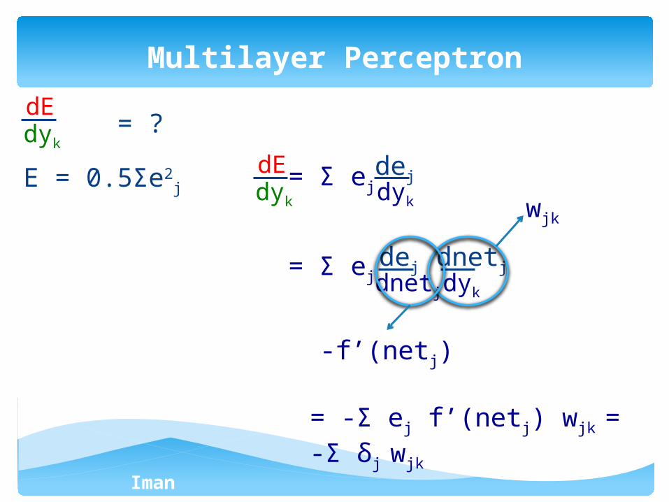
= ?
E = 0.5Σe2j
Multilayer Perceptron
dEdyk
dEdyk
dejdyk
dejdnetj
dnetjdyk
wjk
-f’(netj)
= -Σ ej f’(netj) wjk = -Σ δj wjk
= Σ ej
= Σ ej
Iman Ardekani
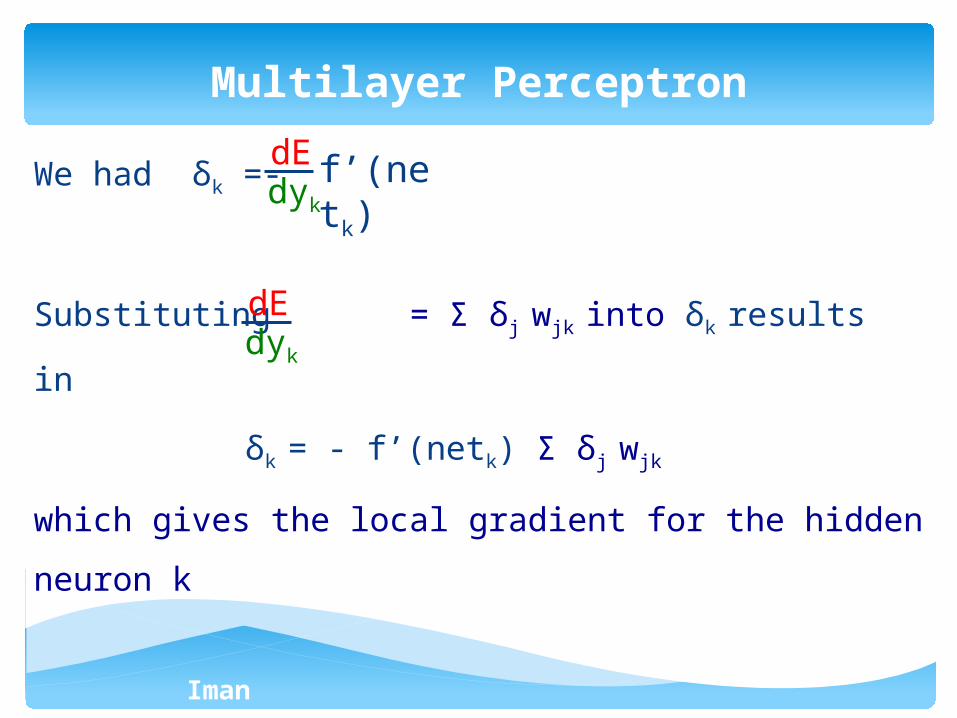
We had δk =-
Substituting = Σ δj wjk into δk results in
δk = - f’(netk) Σ δj wjk
which gives the local gradient for the hidden neuron k
Multilayer Perceptron
dEdyk
f’(netk)
dEdyk
Iman Ardekani
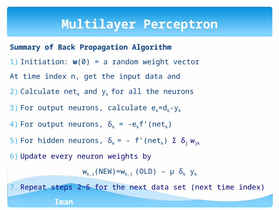
Summary of Back Propagation Algorithm
1) Initiation: w(0) = a random weight vector
At time index n, get the input data and
2) Calculate netk and yk for all the neurons
3) For output neurons, calculate ek=dk-yk
4) For output neurons, δk = -ekf’(netk)
5) For hidden neurons, δk = - f’(netk) Σ δj wjk
6) Update every neuron weights by
wk,i(NEW)=wk,i (OLD) – μ δk yk
7. Repeat steps 2~6 for the next data set (next time index)
Multilayer Perceptron

Iman Ardekani
THE END