artificial neural networks - polimi.it
TRANSCRIPT

© Davide Manca – Dynamics and Control of Chemical Processes – Master Degree in ChemEng – Politecnico di Milano 1L5—
Artificial Neural Networks
Davide Manca
Lecture 5 of “Dynamics and Control of Chemical Processes” – Master Degree in Chemical Engineering

© Davide Manca – Dynamics and Control of Chemical Processes – Master Degree in ChemEng – Politecnico di Milano 2L5—
Introduction
• ANN: Artificial Neural Network
• An ANN is an engine designed to simulate the operation of
the human brain. It is physically implemented with electronic
components or simulated on digital computers via software (Haykin, 1999).
• The ANN consists of simple elements (neurons, nodes, units).
• The information, i.e. the signals, flows through the neurons by means of
connections.
• The connections are weighed to adjust the information flow.
• The information, the weighed signals, is loaded in the neurons and an activation
function also known as transfer function (either linear or non-linear) transforms it
into the output signal.

© Davide Manca – Dynamics and Control of Chemical Processes – Master Degree in ChemEng – Politecnico di Milano 3L5—
The biological neuron
• The central part of the neuron, the nucleus, sums the input signals coming from the
synapses, which are connected to the dendrites of other neurons. When the signal
reaches a limit threshold the neuron produces an output signal towards other
neurons. In other words, the neuron “fires”.
Dendrites
Axon Informationflow
Nucleus
Terminals
Output signal
Input signal from another neuron
Synaptic connections
Input signal from another neuron

© Davide Manca – Dynamics and Control of Chemical Processes – Master Degree in ChemEng – Politecnico di Milano 4L5—
The abstract neuron
x1
x2
xm
...
w1k
w2k
wmk
... j(nk)
Activationfunction
Biasbk
Synapticweights
Inputsignals
Outputsignalyk
nkS
1
m
k jk j
j
w x
( )k ky j n( )kkk b n

© Davide Manca – Dynamics and Control of Chemical Processes – Master Degree in ChemEng – Politecnico di Milano 5L5—
A comparison of neurons and transistors
• The basic unit of the human brain is the neuron.
• The basic unit of a processor, CPU, is the transistor.
• Characteristic times:
neuron 10-3 s;
transistor 10-9 s.
• Energetic consumption for a single operation:
neuron 10-16 J;
transistor 10-7 J.
• Number of basic elements:
in the brain 1010 neurons;
in a processor 109 transistors;
• Synapses number (interconnections) in the human brain: 60,000 billion.
• The brain can be compared to a complex system, for the information processing,
that is highly non-linear and parallel.

© Davide Manca – Dynamics and Control of Chemical Processes – Master Degree in ChemEng – Politecnico di Milano 6L5—
More in depth…
• An ANN may be considered as a system capable of producing an answer to a
question or provide an output after an input data.
• The input output link, which is the transfer function of the network, is not
explicitly programmed. On the contrary, it is simply obtained through a learning
process grounded on empirical data.
• Under the supervised method, the learning algorithm modifies the characteristic
parameters, i.e. weights and biases, so to bring the network forecast near to the
supplied real experimental values.
• Therefore, the main features of the network come close to those of the brain:
capability to learn from the experience (measure of in-the-field data);
high flexibility to interpret the input data (i.e. “noise resistance” or “capability
to interpret noisy data”);
fair extrapolation capability.

© Davide Manca – Dynamics and Control of Chemical Processes – Master Degree in ChemEng – Politecnico di Milano 7L5—
• The ANN history begins with McCulloch e Pitts in 1943.
McCulloch was a psychiatrist and a neuro-anatomist,
whilst Pitts was a mathematician.
The collaboration of these researchers took to the description of the logic calculus of
the neural network, which combines neurophysiology to mathematical logics.
• In 1949 Hebb postulated the first law of self-organized learning (i.e. learning
without a trainer/teacher).
• In 1958 Rosenblatt, in his perceptron work, proposed the first model of supervised
learning (i.e. learning with a trainer/teacher).
• The perceptron introduced by Rosenblatt laid the foundations for the following
neural networks, which can learn any kind of functional dependency.
• In 1969 Minsky and Papert showed mathematically that there are some basic limits
to the learning capability of a single neuron. This result took the scientific
community to temporarily leave the ANN research.
• In the ‘80 of last century, the ANN gained new interest after the introduction of one
or more intermediate levels. Such ANNs, capable of fixing their own errors,
surpassed the perceptron limits of Rosenblatt and revitalized the research in that
sector.
The history

© Davide Manca – Dynamics and Control of Chemical Processes – Master Degree in ChemEng – Politecnico di Milano 8L5—
1. Non-linearity: the presence of non-linear activation functions makes the network
intrinsically non-linear.
2. Analysis and design uniformity: the neurons are a common ingredient for ANNs.
This makes viable sharing both learning theories and algorithms in different
application fields.
3. Input-output map: the network learns by examples based on a sequence of input-
output data (i.e. supervised learning). No a priori assumption is made on the model
parameters.
4. Adaptivity: the ANN can adapt its weights to the changes of the surrounding
environment. In particular, an ANN trained to operate in a given environment, can
be trained again to operate in another one. In addition, if the network is operated in
a dynamically evolving environment, it can be designed to change/modify its
weights in real-time (e.g., adaptive elaboration of the signals, adaptive control).
5. Parallelism: thanks to its structure, an ANN can be implemented directly at the
hardware level for specific high-efficiency computational purposes.
Main features

© Davide Manca – Dynamics and Control of Chemical Processes – Master Degree in ChemEng – Politecnico di Milano 9L5—
Main features
6. Fault tolerant: an hard-wired ANN shows a good tolerance to faults. Its performance
deteriorates slowly in case of malfunctions. This is due to the high relocation of the
information among the neurons, which reduces the risk of catastrophic faults and
guaranties a gradual deterioration of its performance.
7. Neuro-biological analogy: the ANN design is motivated by its analogy with the
human brain that is the living proof that the parallel, fault tolerant, computation is
not only physically viable, but also fast and powerful.

© Davide Manca – Dynamics and Control of Chemical Processes – Master Degree in ChemEng – Politecnico di Milano 10L5—
Network features
• There are three issues that describe and
characterize an ANN:
network architecture. Structure and typology
of the node connections, number of
intermediate levels;
learning method. Evaluation of the intensity
of the node connections (weights and
biases computation);
functional dependency the link the input
to the output of the neuron.
Activation function typology.
© Davide Manca – Dynamics and Control of Chemical Processes – Master Degree in ChemEng – Politecnico di Milano 11L5—
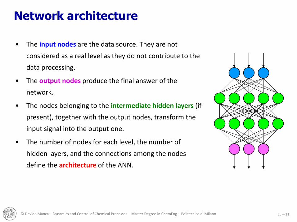
Network architecture
• The input nodes are the data source. They are not
considered as a real level as they do not contribute to the
data processing.
• The output nodes produce the final answer of the
network.
• The nodes belonging to the intermediate hidden layers (if
present), together with the output nodes, transform the
input signal into the output one.
• The number of nodes for each level, the number of
hidden layers, and the connections among the nodes
define the architecture of the ANN.

© Davide Manca – Dynamics and Control of Chemical Processes – Master Degree in ChemEng – Politecnico di Milano 12L5—
Network architecture
• There are several ANN typologies:
networks without hidden layers, i.e. input-output networks;
networks with one or more hidden layers;
fully connected networks;
partially connected networks;
purely feedforward networks, unidirectional flow;
recursive networks with feedback flow;
stationary networks;
adaptive networks, with dynamic memory;
…

© Davide Manca – Dynamics and Control of Chemical Processes – Master Degree in ChemEng – Politecnico di Milano 13L5—
Network architecture
• The most basic structure of an ANN consists of:
one input layer;
one or more hidden layers;
one output layer.
• Every layer has a variable number of nodes. Often, the whole ANN structure is
triangular moving from the top (input) to the bottom (output).
• Cybenko, 1989, showed that a single hidden layer is sufficient to describe any
continuous function.
• Haykin, 1992 (1999), added that the choice of a single hidden layer does not always
produce the best possible configuration (mainly in case of identification of highly
non-linear processes).
George Cybenko Simon Haykin

© Davide Manca – Dynamics and Control of Chemical Processes – Master Degree in ChemEng – Politecnico di Milano 14L5—
Learning methods
• The network training, which consists in adjusting (i.e. evaluating) the optimal
synaptic weights, can happen according to two distinct methods:
SUPERVISED TRAINING (with trainer/teacher)
• During the training, a trainer/teacher supplies the correct answers respect to an input
data set.
• The weights are modified as a function of the error made by the network respect to
the real output data.
External environment
Trainer
ANN S
+
Error signal

© Davide Manca – Dynamics and Control of Chemical Processes – Master Degree in ChemEng – Politecnico di Milano 15L5—
Learning methods
UNSUPERVISED TRAINING (without trainer/teacher)
• There is not a trainer/teacher. Therefore, the feedback contribution is missing.
• The network discovers independently the correlations among the supplied input data.
• The weights change along the training procedure according to an a priori rule which
does not use the error respect the real environment (i.e. process).
• The method uses a measure that is independent of the specific problem.
• Some heuristic rules may be used to transform the external input signal into either an
“award” or a “punishment”.
Externalenvironment
ANN

© Davide Manca – Dynamics and Control of Chemical Processes – Master Degree in ChemEng – Politecnico di Milano 16L5—
Activation function
• The activation function, j(n), defines the neuron output as a function of the activity
level of its inputs.
• Step (or threshold)
function
• Linear piece-wise
(or ramp) function
1
m
k jk j
j
w x
( )k ky j n( )kkk b n
( )1 0
0 0
nj n
n
( )
1 1 2
1 2 1 2
0 1 2
n
j n n n
n
- -

© Davide Manca – Dynamics and Control of Chemical Processes – Master Degree in ChemEng – Politecnico di Milano 17L5—
Activation function
• Sigmoid function
• Hyperbolic tangent
function
N.B.: the activation functions take over values belonging to the 0,…1 or -1,…1
intervals. This is consistent with the fact that the inputs to the network are
normalized to keep limited and controlled the signals flowing in the network.
( )( )
1
1 expj n
n
-
( )( )
( )
1 expTh
2 1 exp
nnj n
n
-

© Davide Manca – Dynamics and Control of Chemical Processes – Master Degree in ChemEng – Politecnico di Milano 18L5—
BP learning
• The most renowned method for supervised training is
the Error Back Propagation Algorithm, BP.
• This algorithm comprises two phases:
forward phase;
backward phase;
• In the forward phase, the learning patterns
(i.e. input-output data pairs) are presented to the
input nodes. The network response depends on the
hidden layer(s) downwards the output nodes. During this phase both weights and
biases remain constant (i.e. unchanged).
• In the backward phase, the error between the real process and the network output
is first evaluated and then back propagated (upwards) through the nodes of the
different layers. Suitable update formula modify the weights and biases up to the
first input layer of the network.

© Davide Manca – Dynamics and Control of Chemical Processes – Master Degree in ChemEng – Politecnico di Milano 19L5—
BP learning
• Somehow, the weights update along the training
procedure may be seen as a parameter regression
that is the optimization of an objective function that
minimizes the average error made on the set of
learning patterns.
• A critical point is the overfitting problem (aka overlearning).
The risk is that the network learns in an optimal way the input-output patterns
provided along the training procedure and loses the generalization capability to deal
with input data that have not been supplied yet.
• A validation procedure of the training procedure
(cross-validation) is mandatory. This is based on a
set of input-output patterns different from that
used during the training procedure.
© Davide Manca – Dynamics and Control of Chemical Processes – Master Degree in ChemEng – Politecnico di Milano 20L5—
Further parameters
• The training procedure is based on two further parameters, both limited in the 0,…1
interval:
learning rate, a
• it determines the learning rate of the ANN: high values increase the learning process
but may bring on convergence problems and instability.
momentum factor, b
• it accounts for the dynamic evolution
of the weights: its role consists in increasing
the procedure velocity while keeping high values
of the learning rate without incurring into
oscillations and convergence problems.

© Davide Manca – Dynamics and Control of Chemical Processes – Master Degree in ChemEng – Politecnico di Milano 21L5—
An example
Neural network type: Back propagation with momentum factorActivation function: Logistic sigmoid + linear functionLearning Algorithm : History Stack Adaptation
4 ! Layers number (including input and output layers)2 ! Neurons number at level: 14 ! Neurons number at level: 22 ! Neurons number at level: 31 ! Neurons number at level: 4
---------------------------------------------------------200 ! Total learning patterns.50000000 ! alfa.90000000 ! beta.10000000 ! mu
---------------------------------------------------------Biases for each layerLayer n. 2 -1.10191428411417 -.306607804280631 .396983628052738 .229701066848763E-01 Layer n. 3 1.32438158863708 .895365411961350Layer n. 4 12.1461254510109---------------------------------------------------------Weights for each layerLayer n. 1 --> 2-.522050637568751 .247668247408662 1.36848442775682 .784256667945155 -2.36688633725843 -2.47312321369078 1.81072640204618 .871974901958030Layer n. 2 --> 31.78023653514858 1.68340336532185-.751951327532474 .906457768573295-1.66948863690154 -.743060896398274-.766335553627057 -.263315123659310Layer n. 3 --> 4-4.61959708139503 -2.87806024443973
End of neural network---------------------------------------------------------

© Davide Manca – Dynamics and Control of Chemical Processes – Master Degree in ChemEng – Politecnico di Milano 22L5—
Identification algorithms
• LOCAL SEARCH
First order methods
• Gradient (steepest descent)
• rather simple;
• possible local minima;
• possible divergence along the search.
Second order methods
• Levenberg-Marquardt
• more complex;
• possible local minima;
• higher memory allocation;
• longer training times;
• deeper minimization of the objective function.

© Davide Manca – Dynamics and Control of Chemical Processes – Master Degree in ChemEng – Politecnico di Milano 23L5—
Identification algorithms
• GLOBAL SEARCH
Simulated Annealing;
Genetic algorithms;
Tabu search;
Multidimensional specific methods (robust methods).
Features:
• complex implementation;
• high cost in terms of memory and CPU time;
• Identification of the global minimum.

© Davide Manca – Dynamics and Control of Chemical Processes – Master Degree in ChemEng – Politecnico di Milano 24L5—
Training methods
• Once the learning set is available, it is time for the network training.
• The provision/implementation of a whole set of patterns is called epoch.
• The training is based on the iterative provision of the epochs according to a stochastic sequence of the patterns to avoid any specific learning and any loss of generality.
• PATTERN MODE training
The update of both weights and biases is made after every supplied pattern to the network. Every pattern undergoes a forward and backward procedure. If a training set comprises N patterns, then there are N weight and bias updates for each epoch.
• BATCH MODE training
The update of both weights and biases is made only after having supplied all the patterns that is at the end of the epoch. The forward procedure supplies Npatterns. The N local errors are stored together with their local gradients. Eventually, these values are averaged and the backward procedure is carried out.

© Davide Manca – Dynamics and Control of Chemical Processes – Master Degree in ChemEng – Politecnico di Milano 25L5—
Convergence criteria
There are not universal criteria to assess the network learning.
• It is worth focusing the attention on the identification degree respect to the set of
the training pattern. For instance, it is possible to check:
If the weights and biases vary a little from an iteration and the following one;
The average error;
The decrease of the average error from an iteration and the following one.
• The real risk for these control
techniques of convergence
is the overfitting of
the network.

© Davide Manca – Dynamics and Control of Chemical Processes – Master Degree in ChemEng – Politecnico di Milano 26L5—
Overfitting examples
• Network of simulated moving-bed reactors for the methanol synthesis.

© Davide Manca – Dynamics and Control of Chemical Processes – Master Degree in ChemEng – Politecnico di Milano 27L5—
Convergence criteria
• It is worth focusing on the identification quality respect to the set of validation
patterns. The average error is checked respect to the validation data set rather than
the learning data set.
error
epochs
learning set
validation set
Epoche (log)
13° epoca 31° epoca

© Davide Manca – Dynamics and Control of Chemical Processes – Master Degree in ChemEng – Politecnico di Milano 28L5—
Overfitting removal
• Network of simulated moving-bed reactors for the methanol synthesis.

© Davide Manca – Dynamics and Control of Chemical Processes – Master Degree in ChemEng – Politecnico di Milano 29L5—
Static and dynamic approach
• An ANN can identify the link (i.e. dependency) between the input and output
variables of the black-box process.
• The input-output dependency may refer to some stationary conditions or better to
some functional dependencies that do not depend neither explicitly nor implicitly
on the time.
• In turn, the network can identify the dynamic behavior of a process. In this case, the
network must be able to describe the system dynamics respect to external
disturbances on the input variables.
• As it happens for the ARX, ARMAX, and NARX systems, the input variables to the
network are not only those of the process inputs but there are also some output
variables referred to past values.
ˆ( ) ( 1), ( 2),......, ( ), ( 1 ), ( 2 ),......., ( )a bk k k k k k k - - - - - - - - -y y y y n u u u nj
Model forecast
Process output
Time delay

© Davide Manca – Dynamics and Control of Chemical Processes – Master Degree in ChemEng – Politecnico di Milano 30L5—
Dynamic identification of processes
• Example: Steam Reforming process.
CH4 + H2O CO + 3H2 DH = +206 kJ/mol
CO + H2O CO2 + H2 DH = -41 kJ/mol
camino ventilatore
ingresso acqua
uscita acqua
alimentazione
bruciatori
ausiliari
ingresso
vapore
uscita
vapore
ingresso vapore
uscita vapore
bruciatori
ingresso acqua
Network input: manipulated variables and measurable disturbances
Network output: controlled variables
naturalgas
Furnace
TTTT
Control System
FT
setpoint
fuelsteam
exhaust
syn-gas
FT
Special Cr/Ni alloy pipes resistant up to 1150 °C.Granular catalyst: Nickel supported on Alumina.

© Davide Manca – Dynamics and Control of Chemical Processes – Master Degree in ChemEng – Politecnico di Milano 31L5—
Open-loop analysis of the system
Hydrogen flowrate [kmol/s]
Disturbance on the furnace fuel flowrate
time [min]
10 15 20 25 30
time [min]
2.48e-03
2.52e-03
2.56e-03
2.60e-03
2.64e-03
2.68e-03
10 15 20 25 30
Disturbance on the dry flowrate
Main features of the process to be identified:
Overshoot presence, slow dynamics, and fast dynamics.

© Davide Manca – Dynamics and Control of Chemical Processes – Master Degree in ChemEng – Politecnico di Milano 32L5—
Open-loop analysis of the system
N.B.: a disturbance on the inlet gas temperature has a delayed effect on the
outlet gas temperature from the reactor. It is necessary to account for this
delay in the definition of the ANN structure in terms of time delay, .
1036
1038
1040
1042
1044
1046
1048
1050
1052
1054
1056
10 15 20 25 30 35
time - min
Outlet gas temperature [K]
Step on the inlet temperature
Step on the fuel flowrate
Step start

© Davide Manca – Dynamics and Control of Chemical Processes – Master Degree in ChemEng – Politecnico di Milano 33L5—
• ANN features: two separate (and dedicated) MISO networks.
N.B.: the second MISO network implements (instead of the reactor outlet
temperature) the produced hydrogen flowrate as output variable.
PC
k-3
1 2
PV
k-3
PS
k-3
3
Tin
k-6
4
Tout
k-3
5
PC
k-2
6
PV
k-2
7
PS
k-2
8
Tin
k-5
9
Tout
k-2
10
PC
k-1
11
PV
k-1
12
PS
k-1
13
Tin
k-4
14
Tout
k-1
15
1
Tout
k
ANN
PC : portata di combustibile
PV : portata di vapore
PS : portata di secco
Tin : temperatura di ingresso
Tout: temperatura di uscita
Dynamic identification of a system

© Davide Manca – Dynamics and Control of Chemical Processes – Master Degree in ChemEng – Politecnico di Milano 34L5—
Bibliography
• Battiti R., First and Second Order Methods for Learning: Between Steepest Descent and Newton's Method,
Neural Computation, 4, 2, 1992
• Cholewo T.J., J.M. Zurada, Exact Hessian Calculation in Feedforward FIR Neural Networks, IEEE International
Joint Conference on Neural Networks, 1998
• Churchland P.S., T.J. Sejnowski, The Computational Brain, MIT Press, Cambridge, 1992
• Cybenko G., Approximation by Superpositions of a Sigmoidal Function, Mathematics of Control Signals and
Systems, 1989
• Hagan M.T., H.B. Demuth, M. Beale, Neural Network Design, PWS Publishing Company, Boston, 1996
• Haykin S., Neural Networks: a Comprehensive Foundation, Prentice-Hall, Upper Saddle River, New Jersey,
1999
• Henson M.A., D.E. Seborg, Nonlinear Process Control, Prentice Hall, 1998
• Hilgard E.R., R.L. Atkinson, R.C. Atkinson, Introduction to Psychology, Harcourt Brace Jovanovich, 1979
• Hrycej T., Neurocontrol towards an Industrial Control Methodology, John Wiley & Sons, New York, 1997
• Narendra K.S., A.U. Levin, Identification using Feedforward Networks, Neural Computation, 7, 1995

© Davide Manca – Dynamics and Control of Chemical Processes – Master Degree in ChemEng – Politecnico di Milano 35L5—
Bibliography
• Narendra K.S., K. Parthasarathy, Identification and Control of Dynamical Systems Using Neural Networks, IEEE
Trans. on Neural Networks, 1, 1990
• Principe J. C., Euliano N. R. and Lefebvre W. C., Neural and Adaptive Systems: Fundamentals through
Simulations, John Wiley & Sons, New York, 2000
• Ranga Suri N.N.R., D. Deodhare, P. Nagabhushan, Parallel Levenberg-Marquardt-based Neural Network
Training on Linux Clusters - A Case Study, Indian Conference on Computer Vision Graphics and Images
Processing, 2002
• Scattolini R., S. Bittanti, On the Choice of the Horizon in Long-range Predictive Control. Some Simple Criteria,
Automatica, 26, 5, 1999
• Tadé M.O., P.M. Mills, A.Y. Zomaya, Neuro-Adaptive Process Control: a Practical Approach, John Wiley &
Sons, New York, 1996
• Wan E.A., F. Beaufays, Diagrammatic Derivation of Gradient Algorithms for Neural Networks, Neural
Computation, 8, 1, 1996
• Werbos P.J., The Roots of Backpropagation - From Ordered Derivatives to Neural Networks and Political
Forecasting, John Wiley & Sons, New York, 1994
• Wilamowski B.M. , Neural Network Architectures and Learning, IEEE-Neural Networks Society, 2003
• Wilamowski B.M., S. Iplikci, O. Kaynak, An Algorithm for Fast Convergence in Training Neural Networks, IEEE
International Joint Conference on Neural Networks, 2001