Artificial Neural Networks

Introduction

Biological Inspirations

Humans perform complex tasks like vision, motor control, or language understanding very well

One way to build intelligent machines is to try to imitate the (organizational principles of) human brain

Human Brain

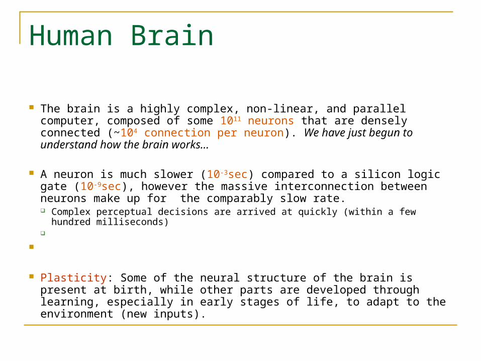
The brain is a highly complex, non-linear, and parallel computer, composed of some 1011 neurons that are densely connected (~104 connection per neuron). We have just begun to understand how the brain works...

A neuron is much slower (10-3sec) compared to a silicon logic gate (10-

9sec), however the massive interconnection between neurons make up for the comparably slow rate. Complex perceptual decisions are arrived at quickly (within a few hundred milliseconds)

Plasticity: Some of the neural structure of the brain is present at birth, while other parts are developed through learning, especially in early stages of life, to adapt to the environment (new inputs).

Human Brain

Some of the neural structure of the brain is present at birth, while other parts are developed through learning, especially in early stages of life, to adapt to the environment (new inputs).

sensory input Integration (learning) motor output

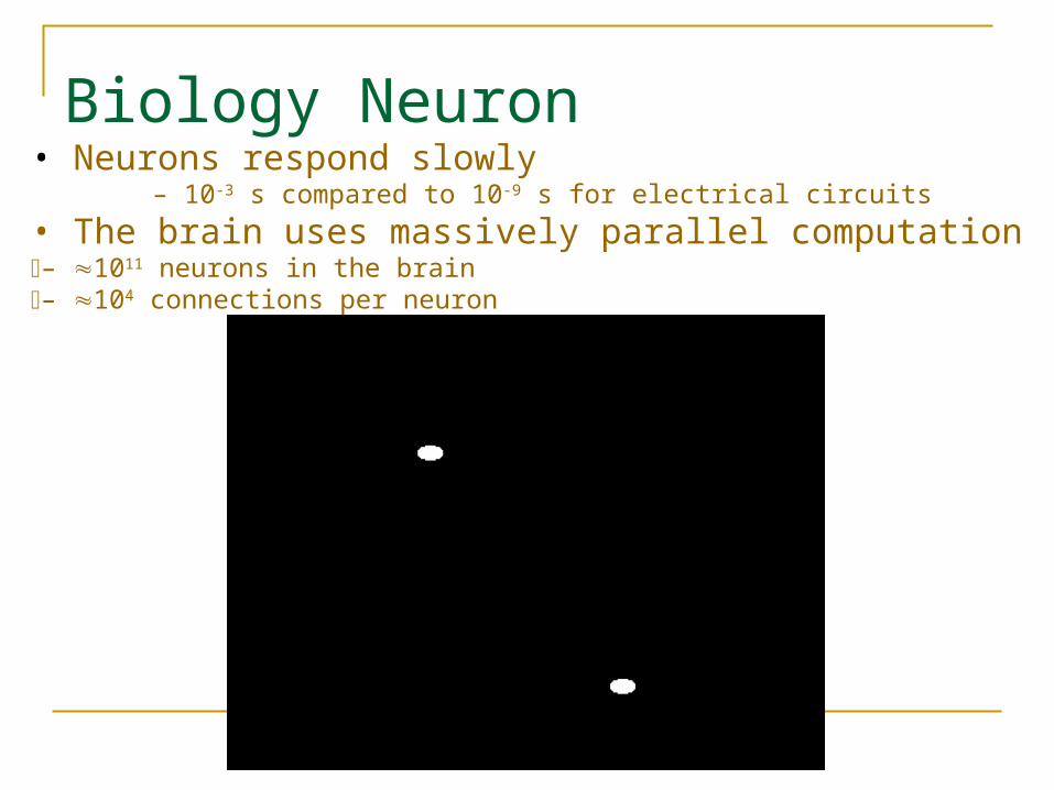
Biology Neuron• Neurons respond slowly

– 10-3 s compared to 10-9 s for electrical circuits

• The brain uses massively parallel computation– 1011 neurons in the brain– 104 connections per neuron

Biological Neuron

Dendrites(樹突 ): nerve fibres carrying electrical signals to the cell

cell body: computes a non-linear function of its inputs

Axon(軸突 ): single long fiber that carries the electrical signal from the cell body to other neurons

Synapse(突觸 ): the point of contact between the axon of one cell and the dendrite of another, regulating a chemical connection whose strength affects the input to the cell.

Biological Neuron

A variety of different neurons exist (motor neuron, on-center off-surround visual cells…), with different branching structures

The connections of the network and the strengths of the individual synapses establish the function of the network.

Artificial Neural Networks

Computational models inspired by the human brain:

Massively parallel, distributed system, made up of simple processing units (neurons)

Synaptic connection strengths among neurons are used to store the acquired knowledge.

Knowledge is acquired by the network from its environment through a learning process

Artificial Neural Networks

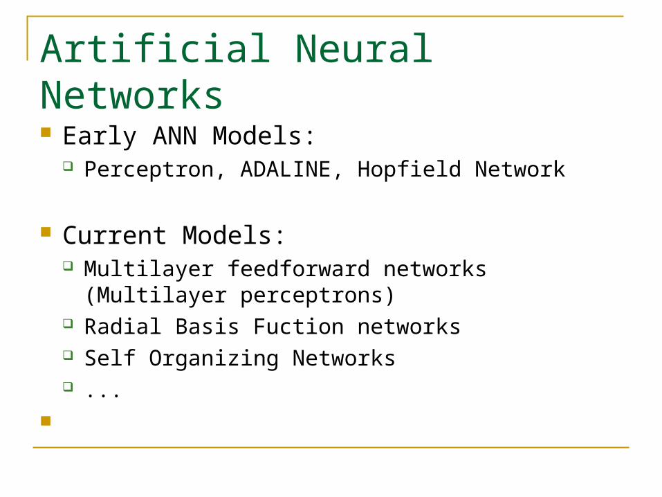
Early ANN Models: Perceptron, ADALINE, Hopfield Network

Current Models: Multilayer feedforward networks (Multilayer

perceptrons) Radial Basis Fuction networks Self Organizing Networks ...

Properties of ANNs

Learning from examples labeled or unlabeled

Adaptivity changing the connection strengths to learn things

Non-linearity the non-linear activation functions are essential

Fault tolerance if one of the neurons or connections is damaged, the whole

network still works quite well

Artificial Neuron Model

Neuroni Activation

x0= +1

x1

x2

x3

xm

wi1

wim

ai

Input Synaptic Output Weights

f

function

bi :Bias

Pre-1940: von Hemholtz, Mach, Pavlov, etc. General theories of learning, vision, conditioning No specific mathematical models of neuron

operation

1940s: Hebb, McCulloch and Pitts Mechanism for learning in biological neurons Neural-like networks can compute any arithmetic

function1958 Rosenblatt->Perceptron

Single-Input Neuron

Bias

n

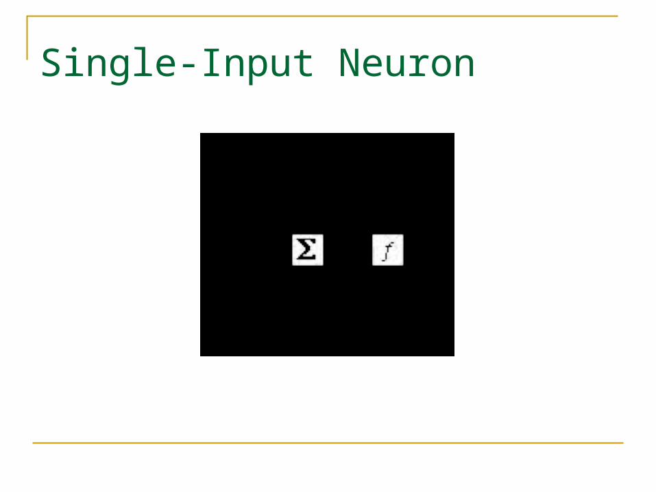
ai = f (ni) = f (wijxj + bi) j = 1

An artificial neuron: - computes the weighted sum of its input and - if that value exceeds its “bias” (threshold), - it “fires” (i.e. becomes active)

Bias

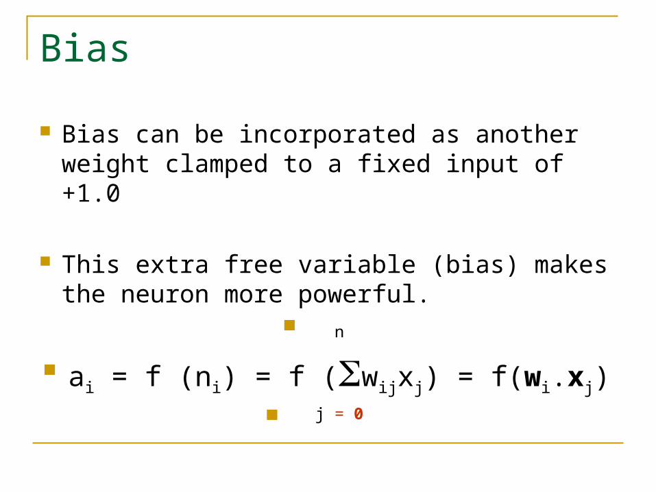
Bias can be incorporated as another weight clamped to a fixed input of +1.0

This extra free variable (bias) makes the neuron more powerful.

n

ai = f (ni) = f (wijxj) = f(wi.xj) j = 0

Activation functions

Also called the squashing function as it limits the amplitude of the output of the neuron.

Many types of activations functions are used:

linear: a = f(n) = n

threshold: a = {1 if n >= 0 (hardlimiting)

0 if n < 0

sigmoid: a = 1/(1+e-n)

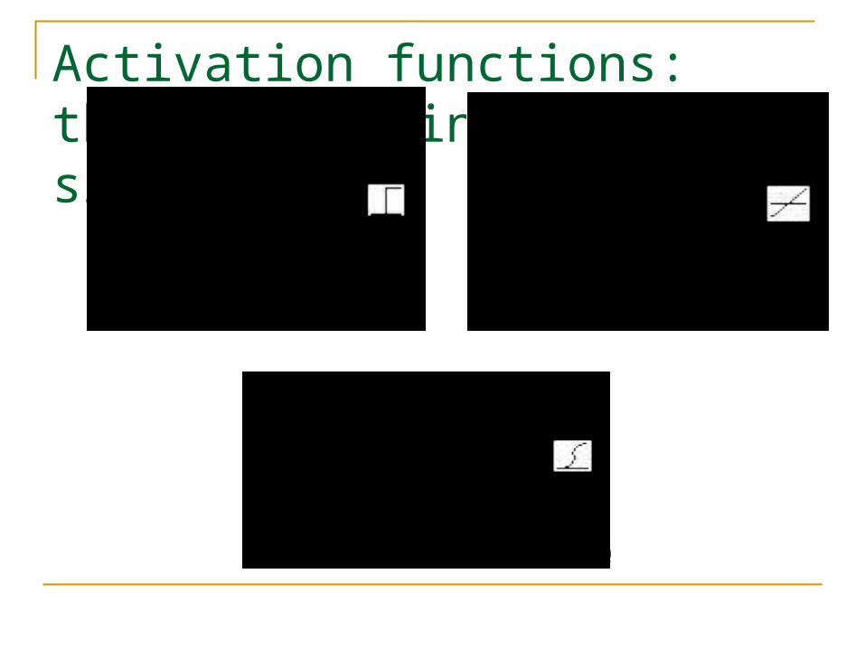
Activation functions: threshold, linear, sigmoid

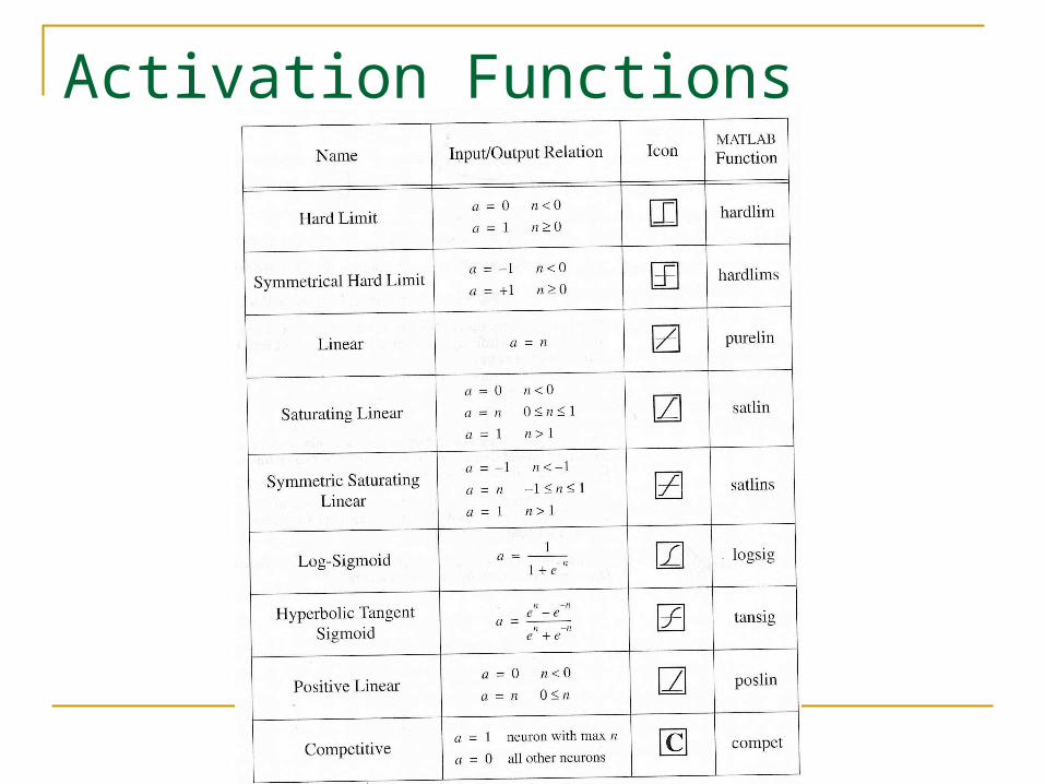
Activation Functions

Ex.

The input to a single-input neuron is 2.0, its weight is 2.3 and its bias is -3.

What is the net input to the transfer function?

What is the neuron output for applying hard limit and linear transfer functions?

sol

The net input: n = wp+b = 2.3*2+(-3) = 1.6

Output for hard limit transfer function a= hardlim(1.6) = 1.6

Output for hard limit transfer function a = purelin(1.6) = 1.6

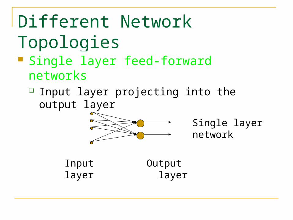
Different Network Topologies

Single layer feed-forward networks Input layer projecting into the output layer

Input Output layer layer

Single layer network

ex

Given a two-input neuron with the following parameters: b = 1.2, w=[3,2], and p = [-5, 6]T,caculate the neuron output for the following transfer functions:

1. A symmetrical hard limit transfer function.

2. A hyperbolic tangent sigmoid transfer function

sol

N = wp+b = [3, 2] + 1.2 = -1.8

1. a = hardlims (-1.8) = -1

2. a = tansig(-1.8) = 0

6

5

ex.

A single-layer neural network is to have six inputs and two outputs. The outputs are to be limited to and continuous over the range 0 to 1. Specify the ANN architecture?

1. how many neurons are required? 2. what are the dimensions of the weight matrix? 3. what kind of transfer functions could be used? Is a bias required?

sol

1. two neurons, one for each output 2. two rows for two neurons, six columns for

six inputs. Logsig Not enough information for bias.

Different Network Topologies

Multi-layer feed-forward networks One or more hidden layers. Input projects

only from previous layers onto a layer.

Input Hidden Output layer layer layer

2-layer or1-hidden layerfully connectednetwork

Different Network Topologies

Recurrent networks A network with feedback, where some of its

inputs are connected to some of its outputs (discrete time).

Input Output layer layer

Recurrentnetwork

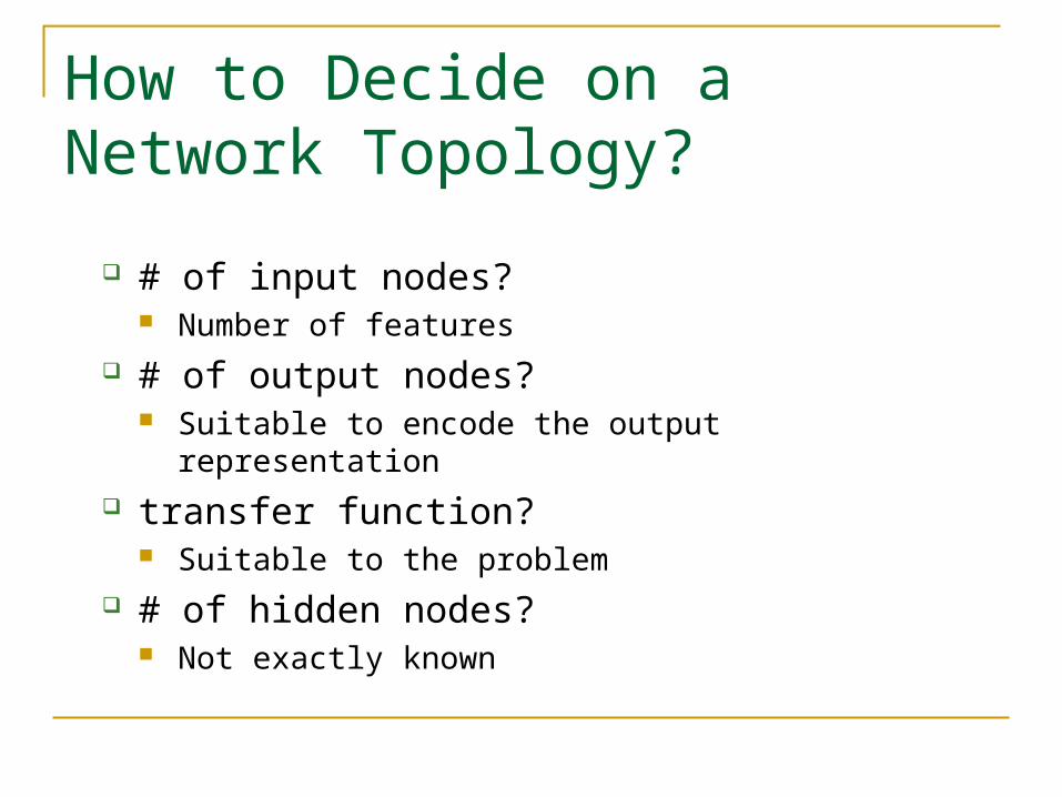
How to Decide on a Network Topology?

# of input nodes? Number of features

# of output nodes? Suitable to encode the output representation

transfer function? Suitable to the problem

# of hidden nodes? Not exactly known

IllustrativeExamples

Boolean OR

p10

0= t1 0=

p20

1= t2 1=

p31

0= t3 1=

p41

1= t4 1=

Given the above input-output pairs (p,t), can you find (manually) the weights of a perceptron to do the job?

Boolean OR Solution

w10.5

0.5=

wT1 p b+ 0.5 0.5

0

0.5b+ 0.25 b+ 0= = = b 0.25–=

2) Weight vector should be orthogonal to the decision boundary.

3) Pick a point on the decision boundary to find the bias.

1) Pick an admissable decision

boundary

Perceptron

Each neuron will have its own decision boundary.

wT

i p bi+ 0=

A single neuron can classify input vectors into two categories.

An S-neuron perceptron can classify input vectors into 2S categories.

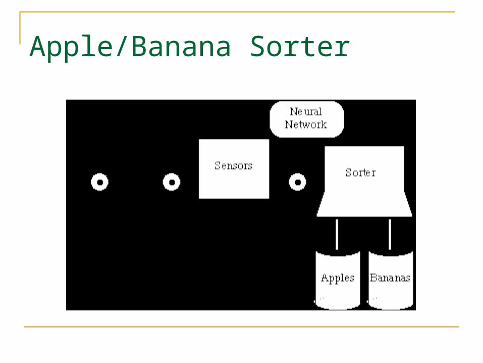
Apple/Banana Sorter

Prototype Vectors

pshape

texture

w eight

=

p2

11

1–

=

Prototype Banana Prototype Apple

Shape: {1 : round ; -1 : eliptical}Texture: {1 : smooth ; -1 : rough}Weight: {1 : > 1 lb. ; -1 : < 1 lb.}

MeasurementVector

p1

1–1

1–

=

Perceptron

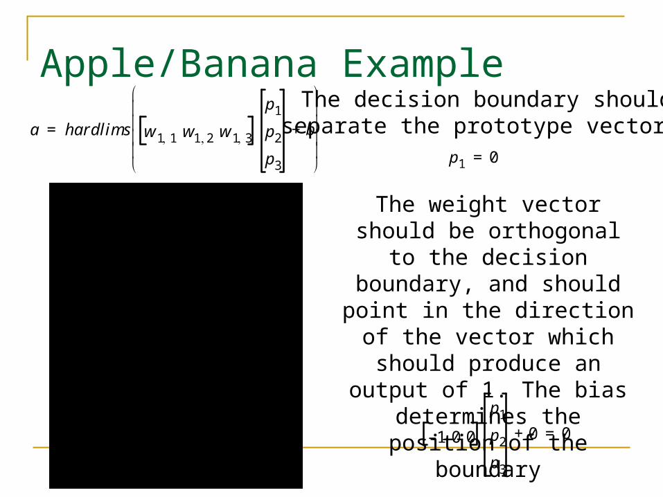
Apple/Banana Example

a hardlims w 1 1 w1 2 w 1 3

p1

p2

p3

b+

=

The decision boundary shouldseparate the prototype vectors.

p1 0=

1– 0 0

p1

p2

p3

0+ 0=

The weight vector should be orthogonal to the decision

boundary, and should point in the direction of the vector which

should produce an output of 1. The bias determines the position

of the boundary

Testing the Network

a har dlims 1– 0 01–1

1–

0+

1 b anana = =

Banana:

Apple:

a hardlim s 1– 0 0

1

1

1–

0+

1– apple = =

“Rough” Banana:

a har dlims 1– 0 01–1–

1–

0+

1 b anana = =

Perceptron Learning Rule

Types of Learning

p1 t1{ , } p2 t2{ , } pQ tQ{ , }

• Supervised Learning (classification)Network is provided with a set of examplesof proper network behavior (inputs/targets)

• Reinforcement Learning (classification)Network is only provided with a grade, or score,which indicates network performance

• Unsupervised Learning (clustering)Only network inputs are available to the learningalgorithm. Network learns to categorize (cluster)the inputs.

Learning Rule Test Problemp1 t1{ , } p2 t2{ , } pQ tQ{ , }

p11

2= t1 1=

p21–

2= t2 0=

p30

1–= t3 0=

Input-output:

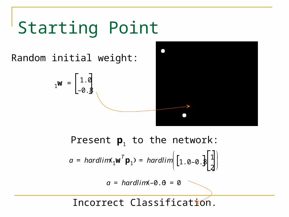
Starting Point

w11.0

0.8–=

Present p1 to the network:

a hardlim wT1 p1 hardlim 1.0 0.8–

1

2

= =

a hardlim 0.6– 0= =

Random initial weight:

Incorrect Classification.

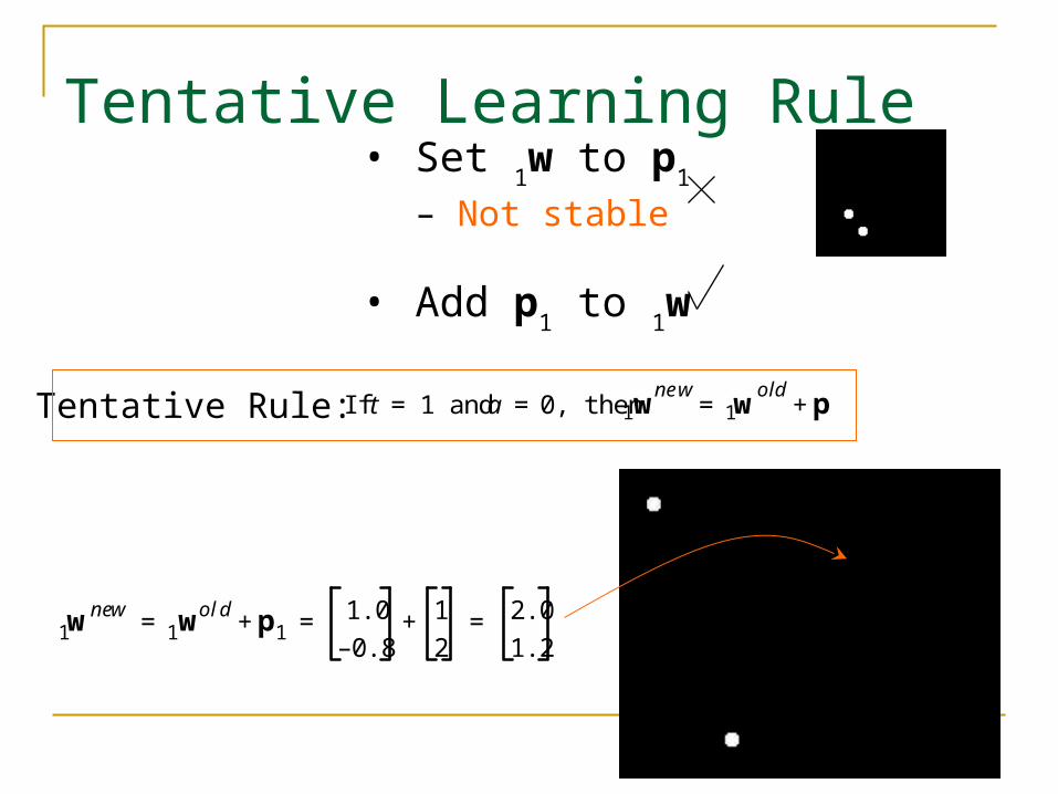
Tentative Learning Rule• Set

1w to p

1

– Not stable

• Add p1 to

1w

If t 1 and a 0, then w1ne w

w1old

p+== =

w1new w1

ol d p1+ 1.0

0.8–

1

2+ 2.0

1.2= = =

Tentative Rule:

Second Input Vector

If t 0 and a 1, then w1ne w

w1old

p–== =

a hardlim wT1 p2 hardlim 2.0 1.2

1–

2

= =

a ha rdlim 0.4 1= = (Incorrect Classification)

Modification to Rule:

w1ne w

w1ol d

p2–2.0

1.2

1–

2–

3.0

0.8–= = =

Third Input Vector

Patterns are now correctly classified.

a hardlim wT

1 p3 hardlim 3.0 0.8–0

1–

= =

a hardlim 0.8 1= = (Incorrect Classification)

w1ne w w1

ol d p3– 3.00.8–

01–

– 3.00.2

= = =

If t a, then w1ne w w1

o ld.==

Unified Learning RuleIf t 1 and a 0, then w1

ne ww1

oldp+== =

If t 0 and a 1, then w1n ew w1

old p–== =

If t a, then w1new w1

ol d==

Unified Learning RuleIf t 1 and a 0, then w1

ne ww1

oldp+== =

If t 0 and a 1, then w1n ew w1

old p–== =

If t a, then w1new w1

ol d==

e t a–=

If e 1, then w1ne w

w1old

p+= =

If e 1,– then w1ne w

w1old

p–==

If e 0, then w1ne w w1

old==

w1new

w1ol d

ep+ w1ol d

t a– p+= =

bne w

bol d

e+=

A bias is a weight with an input of 1.

Define:

=>

Apple/Banana Example

W 0.5 1– 0.5–= b 0.5=

a hardlim Wp1 b+ hardlim 0.5 1– 0.5–1–1

1–

0.5+

= =

Training Set

Initial Weights

First Iteration

p1

1–

11–

t1 1= =

p2

1

11–

t2 0= =

a hardlim 0.5– 0= =

Wne w Wol depT

+ 0.5 1– 0.5– 1 1– 1 1–+ 0.5– 0 1.5–= = =

bne w

bol d

e+ 0.5 1 + 1.5= = =

e t1 a– 1 0– 1= = =

Second Iteration

a hardlim Wp2 b+( ) hardlim 0.5– 0 1.5–11

1–

1.5 +( )= =

a hardlim 2.5( ) 1= =

e t2 a– 0 1– 1–= = =

Wne w WoldepT

+ 0.5– 0 1.5– 1– 1 1 1–+ 1.5– 1– 0.5–= = =

bne w

bol d

e+ 1.5 1– + 0.5= = =

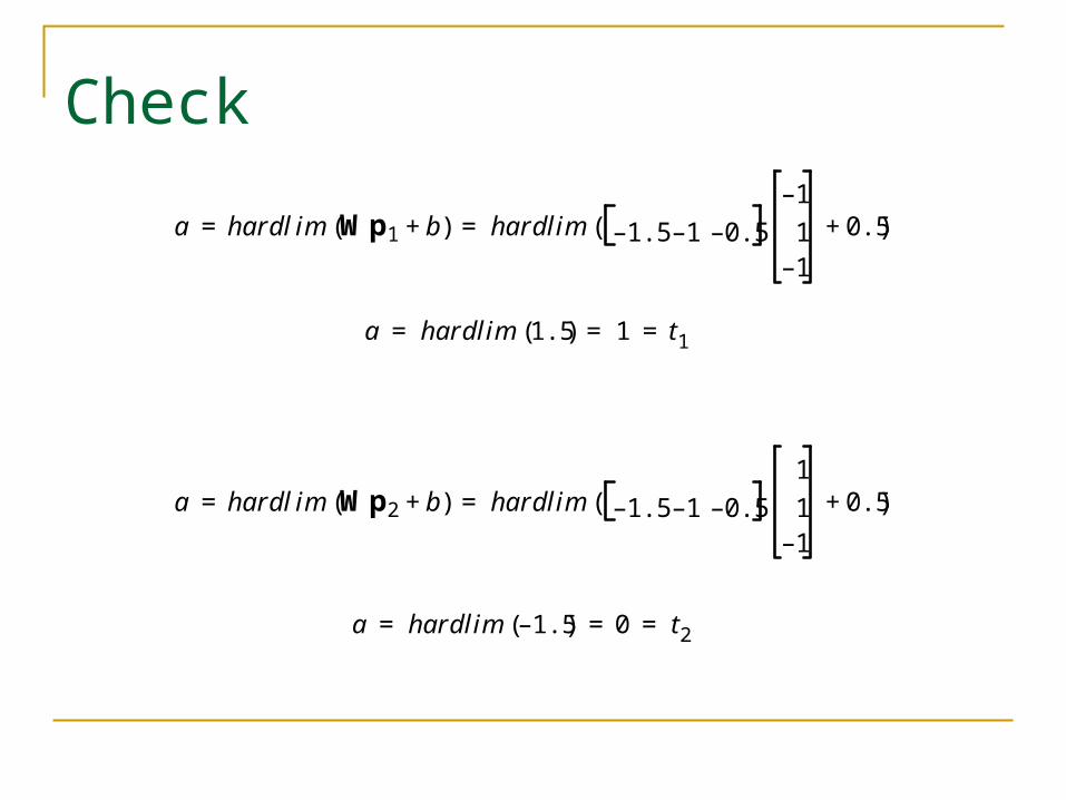
Check

a hardl im Wp1 b+( ) hardlim 1.5– 1– 0.5–

1–

11–

0.5+( )= =

a hardlim 1.5( ) 1 t1= = =

a hardl im Wp2 b+( ) hardlim 1.5– 1– 0.5–

1

11–

0.5+( )= =

a hardlim 1.5–( ) 0 t2= = =

Perceptron Rule Capability

The perceptron rule will always converge to weights which accomplish the desired classification, assuming that

such weights exist.

Perceptron Limitations

wT1 p b+ 0=

Linear Decision Boundary

Linearly Inseparable Problems

Matlab for perceptron ex 4.7

P = [ -0.5 -0.5 +0.3 -0.1; -0.5 +0.5 -0.5 +1.0];

T = [1 1 0 0];

plotpv(P,T)

P defines a 2-element input vectors and a row vector

T defines the vector's target categories.

We can plot these vectors with PLOTPV.

net = newp([-1 1;-1 1],1);plotpv(P,T);plotpc(net.IW{1},net.b{1});

NEWP creates a network object and configures it as a perceptron. The first argument specifies the expected ranges of two inputs. The second determines that there is only one neuron in the layer.

IW(input layer’s initial weight)b (bias’s initial value)

net.adaptParam.passes = 3;

net = adapt(net,P,T);

plotpc(net.IW{1},net.b{1});

net.adaptParam.passes train for 3 times

ADAPT returns a new network object that performs as a better classifier (can use train(net, P, T).

Classify new point

p = [0.7; 1.2];a = net(p);plotpv(p,a);point = findobj(gca,'type','line');set(point,'Color','red'); hold on;plotpv(P,T);plotpc(net.IW{1},net.b{1});hold off;

P = [ -0.5 -0.5 +0.3 -0.1; -0.5 +0.5 -0.5 +1.0];T = [1 1 0 0];plotpv(P,T)

net = newp([-1 1;-1 1],1);plotpv(P,T);plotpc(net.IW{1},net.b{1});

net.adaptParam.passes = 3;net = adapt(net,P,T);plotpc(net.IW{1},net.b{1});

p = [0.7; 1.2];a = net(p);plotpv(p,a);point = findobj(gca,'type','line');set(point,'Color','red');

hold on;plotpv(P,T);plotpc(net.IW{1},net.b{1});hold off;

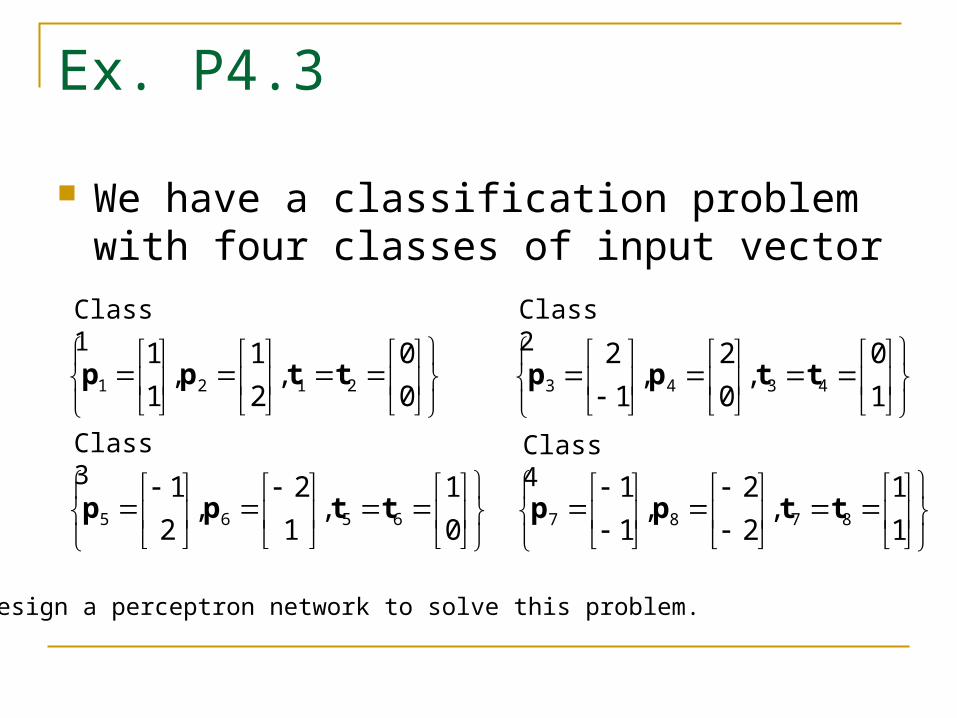
Ex. P4.3

We have a classification problem with four classes of input vector

0

0,

2

1,

1

12121 ttpp

Class 1

1

0,

0

2,

1

24343 ttpp

Class 2

0

1,

1

2,

2

16565 ttpp

Class 3

1

1,

2

2,

1

18787 ttpp

Class 4

Design a perceptron network to solve this problem.

Solved Problem P4.3

(1,2)

(1,1)

(2,0)

(2,1)

(1,2)

(2,1)

(1, 1)

(2, 2)

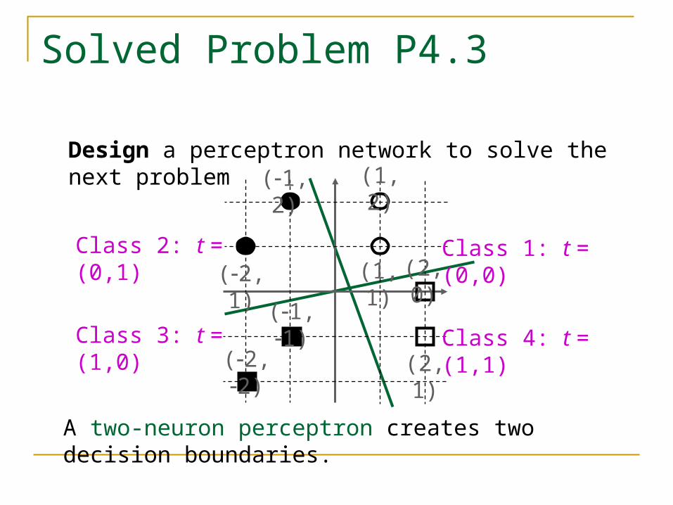
Class 1: t = (0,0)

Class 2: t = (0,1)

Class 4: t = (1,1)

Class 3: t = (1,0)

Design a perceptron network to solve the next problem

A two-neuron perceptron creates two decision boundaries.

Solution of P4.3

0

0,

2

1,

1

12121 ttpp

Class 1

1

0,

0

2,

1

24343 ttpp

Class 2

0

1,

1

2,

2

16565 ttpp

Class 3

1

1,

2

2,

1

18787 ttpp

Class 4

00

021

2

1

11

013

1

3

T222

T111

pww

pww

b

b

0

1 ,

21

13T

2

T1 bw

wW

0

1 ,

21

13T

2

T1 bw

wW

-3

-1

-2

1

1

xin xout

yin yout

P=[1 1 2 2 -1 -2 -1 -2; 1 2 -1 0 2 1 -1 -2];T=[0 0 0 0 1 1 1 1; 0 0 1 1 0 0 1 1];net=newp(minmax(P),2,'hardlim','learnp');%net.IW{1,1}=randn(2);net.IW{1,1}; % you can try net.IW{1,1}=randn(2);%net.b{1}=randn(2,1);net.b{1} % or net.b{1}=randn(2,1); net.adaptParam.passes = 5;net = train(net,P,T);a=sim(net,P);plotpc(net.IW{1, 1},net.b{1}); figure(2); plotpv(P,T); hold on; plotpc(net.IW{1},net.b{1});

Solved Problem P4.5

Train a perceptron network to solve P4.3 problem using the perceptron learning rule.

.1

1)0( ,

10

01)0(

bW

1

1

1

1)0()0(hardlim 11 atebpWa

0

0 ,

1

111 tp

0

0)0()1( ,

01

10)0()1( T

1 ebbepWW

Solution of P4.5

.0

0)1( ,

01

10)1(

bW

0

0

0

0)1()1(hardlim 22 atebpWa

0

0 ,

2

122 tp

.0

0)1()2(

,01

10)1()2( T

2

ebb

epWW

Solution of P4.5

.0

0)2( ,

01

10)2(

bW

1

1

0

1)2()2(hardlim 33 atebpWa

1

0 ,

1

233 tp

.1

1)2()3(

,11

02)2()3( T

3

ebb

epWW

)3()4()5()6()7()8()3()4()5()6()7()8(

bbbbbbWWWWWW

Solution of P4.5

.1

1)8( ,

11

02)8(

bW

0

0 ,

1

111 tp

1

0

1

0)8()8(hardlim 11 atebpWa

.0

1)8()9(

,20

02)8()9( T

1

ebb

epWW

-2

0

-2

0

-1

xin xout

yin yout

Hamming Network

Hamming network was designed explicitly to solve binary (1 or –1) pattern recognition problem.

It uses both feedforward and recurrent (feedback) layers.

The objective is to decide which prototype vector is closest to the input vector.

When the recurrent layer converges, there will be only one neuron with nonzero output.

Hamming Network

a1

S1

n1

S1

+W1

SR

R

pR1

S

1 b1

S1

W2

SS

S

Dn2(t+1)

S1

S1

a2(t+1)

S1a2(t)

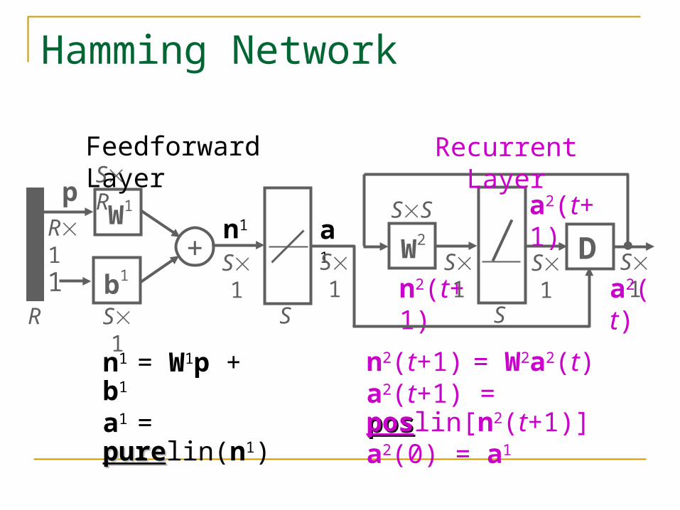
Feedforward Layer Recurrent Layer

n1 = W1p + b1

a1 = purepurelin(n1)n2(t+1) = W2a2(t) a2(t+1) = posposlin[n2(t+1)]a2(0) = a1

Feedforward Layer

The feedforward layer performs a correlation, or inner product, between each of the prototype patterns and the input pattern.

The connection matrix W1 are set to the prototype patterns. Each element of the bias vector b1 is set to be R, such that the

outputs a1 can never be negative.

a1

S1

n1

S1

+W1

SR

R

p

R1

S

1 b1

S1

n1 = W1p + b1

a1 = purepurelin(n1)

Feedforward Layer

The outputs are equal to the inner products of each prototype pattern (p1 and p2) with the input (p), plus R (3).

3

3 ,

111

111 1

2

11 bp

pW

T

T

3

3

3

3

2

1

2

1111

pp

ppp

p

pbpWa

T

T

T

T

P1: a prototype orangeP2: a prototype apple

2

4

3

3

1

1

1

111

111

1

1

1111 bpWap

Feedforward Layer

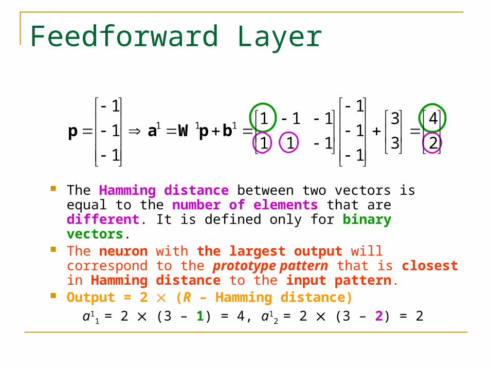
The Hamming distance between two vectors is equal to the number of elements that are different. It is defined only for binary vectors.

The neuron with the largest output will correspond to the prototype pattern that is closest in Hamming distance to the input pattern.

Output = 2 (R – Hamming distance) a1

1 = 2 (3 – 1) = 4, a12 = 2 (3 – 2) = 2

Recurrent Layer

The recurrent layer of the Hamming network is what is known as a “competitive” layer.

The neurons compete with each other to determine a winner. After the competition, only one neuron will have a nonzero output.

n2(t+1) = W2a2(t) a2(t+1) = posposlin[n2(t+1)]a2(0) = a1

W2

SS

S

Dn2(t+1)

S1

S1

a2(t+1)

S1

a2(t)

a1

Recurrent Layer

Each element is reduced by the same fraction of the other. The difference between large and small will be increased.

The effect of the recurrent layer is to zero out all neuron outputs, except the one with the largest initial value (which corresponds to the prototype pattern that is closest in Hamming distance to the input).

1

1 and ,

)(

)()( ,

1

122

2122

Sta

tat

aW

)()(

)()(poslin)(poslin)1(

21

22

22

21222

tata

tatatt

aWa

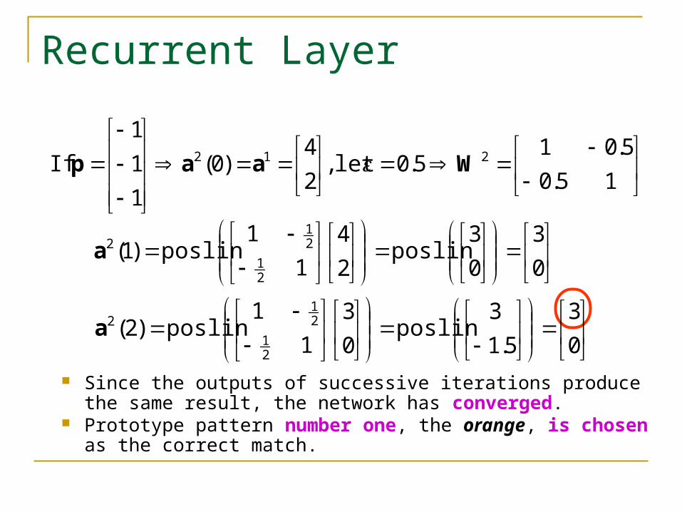
Recurrent Layer

15.0

5.015.0let ,

2

4)0(

1

1

1

If 212 Waap

0

3

0

3poslin

2

4

1

1poslin)1(

21

21

2a

0

3

5.1

3poslin

0

3

1

1poslin)2(

21

21

2a

Since the outputs of successive iterations produce the same result, the network has converged.

Prototype pattern number one, the orange, is chosen as the correct match.