arX

iv:a

stro

-ph/

0301

138v

3 1

9 M

ar 2

003

A&A manuscript no.(will be inserted by hand later)

Your thesaurus codes are:07 (07.09.1; 07.13.1; )

ASTRONOMYAND

ASTROPHYSICS2.4.2018

ELECTROMAGNETIC RADIATION AND

MOTION OF A PARTICLE

J. Klacka

Astronomical Institute, Faculty of Mathematics, Physics and Informatics,

Comenius University, Mlynska dolina, 842 48 Bratislava, Slovak Republic

e-mail: klacka@fmph.uniba.sk

I would like to dedicate this paper to the memory of my sister

Zuzka Klackova (* 5. 7. 1966 †27. 3. 1991)

Abstract. We consider the motion of uncharged dust grains of arbitrary shape including

the effects of electromagnetic radiation and thermal emission. The resulting relativisti-

cally covariant equation of motion is expressed in terms of standard optical parameters.

Explicit expressions for secular changes of osculating orbital elements are derived in de-

tail for the special case of the Poynting-Robertson effect. Two subcases are considered:

(i) central acceleration due to gravity and the radial component of radiation pressure

independent of the particle velocity, (ii) central acceleration given by gravity and the

radiation force as the disturbing force. The latter case yields results which may be com-

pared with secular orbital evolution in terms of orbital elements for an arbitrarily shaped

dust particle. The effects of solar wind are also presented.

Key words: cosmic dust, electromagnetic radiation, thermal emission, relativity theory,

equation of motion, orbital motion, celestial mechanics

2

1. Introduction

Poynting (1904) formulated a problem of finding equation of motion for a perfectly ab-

sorbing spherical particle under the action of electromagnetic radiation. Poynting did not

succeed in finding correct solution. The second case, closely connected with the relativis-

tic equation of motion for a free particle under the action of electromagnetic radiation,

was presented by Einstein (1905), who calculated the change of energy and light pres-

sure at arbitrary angle of incidence on a plane mirror. Robertson (1937) subsequently

derived a correct equation of motion for a perfectly absorbing spherical particle. This

result has been applied to astronomical problems for several decades and is known as

the Poynting-Robertson (P-R) effect. Robertson’s case was relativistically generalized by

Klacka (1992a), who showed that the generalized P-R effect holds only for the special

case where the total momentum of the outgoing radiation per unit time is colinear with

the incident radiation (in the proper/rest frame of reference of the particle), which may

include radiation normally incident on a plane mirror. Since real particles interact with

electromagnetic radiation in a complicated manner and particles of various optical prop-

erties exist (e. g., Mishchenko et al. 2002), it is essential to have an equation of motion

sufficiently general to cover a wide range of optical parameters, not just the limited cases

previously investigated. As an attempt of formulating such a general equation of motion,

we can mention Lyttleton (1976), Klacka (1994a), Klacka and Kocifaj (1994), Kocifaj et

al. (2000). The last three presentations are of hypothetical character only, since none of

them proves correctness of the equation of motion. However, Klacka (2000a) succeeded

in deriving relativistically covariant equation of motion. This equation of motion was

derived in other possible ways by Klacka (2000b), Klacka and Kocifaj (2001), within

the accuracy corresponding to Klacka (1994a). Finally, knowing the results obtained by

Klacka and Kocifaj (1994) and Kocifaj et al. (2000) and having in disposal papers by

Klacka (2000a, 2000b, 2000c), Kimura et al. (2002) presented a repetition of the equation

of motion corresponding to Klacka and Kocifaj (1994) and Kocifaj et al. (2000).

The equations of motion for a moving particle have been constructed under the as-

sumption that thermal emission from a particle is isotropic and does not exert a radiation

pressure force on the particle in the particle frame of reference. Recently, Mishchenko

(2001) has formulated the radiation pressure on arbitrarily shaped particles arising from

an anisotropy of thermal emission. In this paper, we derive the equation of motion for an

arbitrarily shaped particle moving in a radiation field taking into account the radiation

pressure caused by an anisotropy of thermal emission as well as scattering and absorp-

3

tion of light. Relativistically covariant equation of motion is presented. Derivation of the

equation of motion is physically fully reasoned.

We begin by reviewing in Sec. 2 and 3 the basic physical processes in proper and

stationary frames. The equation of motion for simultaneous action of gravity and elec-

tromagnetic radiation is presented in Sec. 4. Sec. 5 then applies these results to the

calculation of osculating orbital elements, including the special case of the P-R effect,

which may be treated analytically. The calculation is carried out in Sec. 6 to first order

in v/c and applied to the ejection of a dust particle from a parent body such as a comet

or asteroid. Two cases are considered: (i) the disturbing acceleration is given in terms of

velocity (Robertson 1937, Wyatt and Whipple 1950), and (ii) the electromagnetic radi-

ation itself is a disturbing function. However, these authors (including Lyttleton 1976)

did not obtain the correct expression for the secular change of longitude of pericenter

(perihelion). In Sec. 7 we use the equation of motion to second order in v/c for the P-R

effect. In particular we obtain a correct expression for the secular change of longitude of

pericenter (perihelion). Sec. 8 then finds the secular change in the advancement of perihe-

lion to first order in v/c, with gravity as a central acceleration. Next, we briefly discuss,

in Sec. 9, the secular evolution of orbital elements for the P-R effect and nearly-circular

orbits. Sec. 10 then treats the effect of the solar wind on the secular changes in the orbital

elements to the second order in v/u, where u is the speed of solar wind particles. Finally,

Sec. 11 summarizes our results.

Other theoretical papers on the basic properties of the P-R effect were written during

the last decades: Burns et al. (1979), Mediavilla and Buitrago (1989), Mignard (1992),

Srikanth (1999), Williams (2002). Some others will be mentioned within the context of

the discussed problems. Since some confusion exists in presenting derivations and results

in the most cited papers (Robertson 1937; Wyatt and Whipple 1950; Burns et al. 1979;

Mignard 1992), we present detailed derivation of the secular changes of orbital elements

for heliocentric orbits and the P-R effect.

2. Proper reference frame of the particle – stationary particle

The term “stationary particle” will denote a particle which does not move in a given

inertial frame of reference. Primed quantities will denote quantities measured in the

proper reference frame of the particle – rest frame of the particle.

The flux density of photons scattered into an elementary solid angle dΩ′ =

sin θ′ dθ′ dφ′ is proportional to p′(θ′, φ′) dΩ′, where p′(θ′, φ′) is the “phase function”.

The phase function depends on orientation of the particle with respect to the direction

4

of the incident radiation and on the particle characteristics; angles θ′, φ′ correspond to

the direction (and orientation) of travel of the scattered radiation, θ′ is the polar angle

which vanishes for propagation along the unit vector e′1 of the incident radiation. The

phase function fulfills the normalisation condition∫

4π

p′(θ′, φ′) dΩ′ = 1 . (1)

The momentum of the incident beam of photons which is lost in the process of inter-

action with the particle is proportional to the cross-section C′ext (extinction). The part

proportional to C′

abs (absorption) is emitted in the form of thermal radiation and the

part proportional to C′ext − C′

abs = C′sca is scattered. The differential scattering cross

section dC′sca/dΩ

′ ≡ C′sca p′(θ′, φ′) depends on the polarization state of the incident light

as well as on the incidence and scattering directions (e. g., Mishchenko et al. 2002).

The momentum (per unit time) of the scattered photons into an elementary solid

angle dΩ′ is

dp′

sca =1

cS′ C′

sca p′(θ′, φ′) K′ dΩ′ , (2)

where the unit vector in the direction of scattering is

K′ = cos θ′ e′1+ sin θ′ cosφ′ e′

2+ sin θ′ sinφ′ e′

3. (3)

S′ is the flux density of radiation energy (energy flow through unit area perpendicular to

the ray per unit time). The system of unit vectors used on the RHS of the last equation

forms an orthogonal basis. The total momentum (per unit time) of the scattered photons

is

p′

sca =1

cS′ C′

sca

∫

4π

p′(θ′, φ′) K′ dΩ′ . (4)

The momentum (per unit time) obtained by the particle due to the interaction with

radiation – radiation force acting on the particle – is

d p′

d t′=

1

cS′

C′

ext e′

1 − C′

sca

∫

4π

p′(θ′, φ′) K′ dΩ′

+ F ′

e(T′) , (5)

where the emission component of the radiation force acting on the particle of absolute

temperature T ′ is (Mishchenko et al. 2002, pp. 63-66)

F ′

e(T′) = − 1

c

∫ ∞

0

dω′

∫

4π

r′ K ′

e

(

r′, T ′, ω′)

dr′ . (6)

The unit vector r′ = r′/r′ is given by position vector r′ of the observation point with

origin inside the particle (the emitted radiation in the far-field zone of the particle prop-

agates in the radial direction, i. e., along the unit vector r′), ω′ is (angular) frequency of

radiation,

5

K ′

e

(

r′, T ′, ω′)

= I ′b (T′, ω′)

[

K ′

11

(

r′, ω′)

−∫

4π

Z ′

11

(

r′, r′′, ω′)

dr′′

]

, (7)

where K ′11

is the (1,1) element of the particle extinction matrix, Z ′11

is the (1,1) element

of the phase matrix and the Planck blackbody energy distribution is given by the well-

known relation

I ′b (T′, ω′) =

h ω′3

4 π3 c2

exp

(

h ω′

k T ′

)

− 1

−1

. (8)

Thermal emission has to be included in the total interaction of the particle with electro-

magnetic radiation: if the particle’s absolute temperature is above zero, it can emit as

well as scatter and absorb electromagnetic radiation.

For the sake of brevity, we will use dimensionless efficiency factors Q′x instead of cross

sections C′x: C

′x = Q′

x A′, where A′ is geometrical cross section of a sphere of volume

equal to the volume of the particle. Equation (5) can be rewritten to the form

d p′

d τ=

1

cS′ A′ [Q′

ext − < cos θ′ > Q′

sca] e′

1+ [ − < sin θ′ cosφ′ > Q′

sca] e′

2+

[ − < sin θ′ sinφ′ > Q′

sca] e′

3 +

3∑

j=1

F ′

ej e′j , (9)

where < x′ >≡∫

4πx′ p′(θ′, φ′) dΩ′ and F ′

ej ≡ F ′e(T

′) · e′j . As for the energy, we assume

that it is conserved: the energy (per unit time) of the incoming radiation E′i, equals to

the energy (per unit time) of the outgoing radiation (after interaction with the particle)

E′o. We will use the fact that time t′ = τ , where τ is proper time.

Summarizing important equations, we can write them in a short form

d p′

d τ=

3∑

j=1

(

S′ A′

cQ′

j + F ′

ej

)

e′j ;d E′

d τ= 0 , (10)

where Q′1 ≡ Q′

ext − < cos θ′ > Q′sca, Q

′2 ≡ − < sin θ′ cosφ′ > Q′

sca, Q′3 ≡ − <

sin θ′ sinφ′ > Q′sca. We have added an assumption of equilibrium state when the parti-

cle’s mass does not change.

2.1. Summary of the important equations

Using the text concerning energy below Eq. (9) and the last Eq. (10), we may describe the

total process of interaction in the form of the following equations (energies and momenta

per unit time):

E′

o = E′

i = A′ S′ ,

p′

o = (1 − Q′

1) p′

i − (Q′

2 e′2 + Q′

3 e′3) E′

o/c −3∑

j=1

F ′

ej e′j ,

p′

i = (E′

i/c) e′

1, (11)

6

The index ”i” represents the incoming radiation, beam of photons, the index ”o” rep-

resents the outgoing radiation. The relation for p′o represents a generalization of the

following cases:

i) Q′1 = 1, Q′

2 = Q′3 = F ′

e1 = F ′e2 = F ′

e3 = 0 – Robertson (1937), Robertson and Noonan

(1968), Srikanth (1999);

ii) Q′1arbitrary, Q′

2= Q′

3= F ′

e1 = F ′e2 = F ′

e3 = 0 – Klacka (1992a);

iii) Q′1, Q′

2, Q′

3arbitrary, F ′

e1 = F ′e2 = F ′

e3 = 0 – Klacka (2000a).

The changes of energy and momentum of the particle due to the interaction with

electromagnetic radiation are

d E′

d τ= E′

i − E′

o = 0 ,

d p′

d τ= p′

i − p′

o . (12)

3. Stationary frame of reference

By the term “stationary frame of reference” (laboratory frame) we mean a frame of

reference in which particle moves with a velocity vector v = v(t). The physical quantities

measured in the stationary frame of reference will be denoted by unprimed symbols.

Our aim is to derive equation of motion for the particle in the stationary frame of

reference. We will use the fact that we know this equation in the proper frame of reference

– see Eqs. (11) and (12).

If we have a four-vector Aµ = (A0,A), where A0 is its time component and A is its

spatial component, generalized special Lorentz transformation yields

A0′

= γ (A0 − v ·A/c) ,

A′ = A + [(γ − 1) v ·A/v2 − γ A0/c] v , (13)

with inverse

A0 = γ (A0′

+ v ·A′/c) ,

A = A′ + [(γ − 1) v ·A′/v2 + γ A0′

/c] v , (14)

where γ = 1/√

1 − v2/c2 .

As for four-vectors we immediately introduce four-momentum:

pµ = (p0,p) ≡ (E/c,p) . (15)

7

3.1. Incoming radiation

Applying Eqs. (14) and (15) to quantity (E′i/c,p

′i) (four-momentum per unit time –

proper time is a scalar quantity) and taking into account also Eqs. (11), we can write

Ei = E′

i γ (1 + v · e′1/c) ,

pi =E′

i

c

e′1+[

(γ − 1) v · e′1/v2 + γ/c

]

v

. (16)

Using the fact that pµ = (h ν, h ν e1) for photons, we have

ν′ = ν w1 ,

e′1 =1

w1

e1 +[

(γ − 1) v · e1/v2 − γ/c]

v

, (17)

where

w1 ≡ γ (1 − v · e1/c) . (18)

Inserting the second of Eqs. (17) into Eqs. (18), one obtains

Ei = (1/w1) E′

i ,

pi = (1/w1) (E′

i/c) e1 . (19)

We have four-vector pµi = (Ei/c,pi) = (1, e1)Ei/c = (1/w1, e1/w1) w1 Ei/c ≡

bµ1w1 Ei/c.

For monochromatic radiation the flux density of radiation energy becomes

S′ = n′ h ν′ c ; S = n h ν c , (20)

where n and n′ are concentrations of photons (photon number densities) in the corre-

sponding reference frames. We also have continuity equation

∂µ jµ = 0 , jµ = (c n, c n e1) , (21)

with current density jµ. Application of Eq. (13) then yields

n′ = w1 n . (22)

Using Eqs. (17), (20) and (22) we finally obtain

S′ = w2

1 S . (23)

Eqs. (11), (19) and (23) then together give Ei = w1 S A′, pi = w1 S A′ e1/c.

8

3.2. Outgoing radiation

The situation is analogous to that of the preceding subsection. It is only a little more

algebraically complicated, since radiation may also spread out in directions given by unit

vectors e2, e3. How can we find transformations for the unit vectors e′2and e′

3? The

crucial point is what physics do these unit vectors describe. The vectors e′2and e′

3can

be used to describe directions of propagation of radiation scattered by the particle. Thus,

aberration of light also exists for each of these unit vectors. The relations between e′2 and

e2, e′3 and e3, are analogous to that presented by the second of Eq. (17):

e′j =1

wj

ej +[

(γ − 1) v · ej/v2 − γ/c]

v

, j = 1, 2, 3 , (24)

where

wj ≡ γ (1 − v · ej/c) , j = 1, 2, 3 . (25)

It is worth mentioning that vectors

e′j ; j = 1, 2, 3

form an orthonormal set of vectors,

and, unit vectors ej ; j = 1, 2, 3 are not orthogonal unit vectors.

Applying Eqs. (14) and (15) to the quantity (E′o/c,p

′o) (four-momentum per unit time

– proper time is a scalar quantity), we can write

Eo = γ (E′

o + v · p′

o) ,

po = p′

o +

[

(γ − 1) v · p′

o/v2 + γ

E′o

c2

]

v . (26)

Using also p′i = E′

i e′1/c and Eqs. (11), (24), (26),

Eo = Q′

1w1 Ei γ + (1 − Q′

1) Ei +

w1 Ei (Q′

2+ Q′

3) γ − w1 Ei (Q

′

2/w2 + Q′

3/w3) −

3∑

j=1

F ′

ej (c/wj − γ c) ,

po = (1 − Q′

1)Ei

ce1 + Q′

1

w1 Ei

c2γ v −

3∑

j=2

Q′

j

w1 Ei

c2(c ej/wj − γ v) −

1

c

3∑

j=1

F ′

ej (c ej/wj − γ v) . (27)

3.3. Equation of motion

In analogy with Eqs. (12), we have for the changes of energy and momentum of the

particle due to the interaction with electromagnetic radiation

d E

d τ= Ei − Eo ,

d p

d τ= pi − po . (28)

9

Putting Eqs. (27) into Eqs. (28), using also pi = (Ei/c) e1, one easily obtains

d E/c

d τ=

3∑

j=1

(

Q′

j

w1 Ei

c2+

1

cF ′

ej

)(

c1

wj− γ c

)

,

d p

d τ=

3∑

j=1

(

Q′

j

w1 Ei

c2+

1

cF ′

ej

) (

cejwj

− γv

)

. (29)

Eq. (29) may be rewritten in terms of four-vectors:

d pµ

d τ=

3∑

j=1

(

Q′

j

w1 Ei

c2+

1

cF ′

ej

)

(

c bµj − uµ)

, (30)

where pµ is four-vector of the particle of mass m

pµ = m uµ , (31)

four-vector of the world-velocity of the particle is

uµ = (γ c, γ v) . (32)

We have also other four-vectors

bµj = (1/wj , ej/wj) , j = 1, 2, 3 . (33)

It can be easily verified that:

i) the quantity w Ei is a scalar quantity – see first of Eqs. (19);

ii) Eq. (30) reduces to Eq. (10) for the case of proper inertial frame of reference of the

particle;

iii) Eq. (30) yields d m/d τ = 0.

We introduce

b0j ≡ 1/wj = γ (1 + v · e′j / c) ,

bj ≡ ej / wj = e′j + [(γ − 1) v · e′j / v2 + γ / c] v , j = 1, 2, 3 (34)

for the purpose of practical calculations. Physics of these relations corresponds to aber-

ration of light.

We have derived an equation of motion for real dust particle under the action of

electromagnetic radiation (including thermal emission). It is supposed that the equation

of motion is represented by Eqs. (11) and (12) in the proper frame of reference of the

particle. The final covariant form is represented by Eq. (30), or using Ei = w1 S A′ (see

Eqs. (11), (19) and (23)),

d pµ

d τ=

3∑

j=1

(

w2

1S A′

c2Q′

j +1

cF ′

ej

)

(

c bµj − uµ)

. (35)

10

Another form of equation of motion is presented in Appendix A. There is also ex-

plained why considerations presented by Kimura et al. (2002) are incorrect.

To first order in v/c, Eqs. (34)-(35) yield

d v

d t=

S A′

m c

3∑

j=1

Q′

j [(1 − 2 v · e1/c + v · ej/c) ej − v/c] +

1

m

3∑

j=1

F ′

ej

[(

1 +v · ejc

)

ej − v

c

]

,

ej = (1 − v · e′j/c) e′j + v/c , j = 1, 2, 3 . (36)

It is worth mentioning to stress that the values of Q′−coefficients depend on particle’s

orientation with respect to the incident radiation – their values are time dependent. A

little different derivation of the equation of motion within the accuracy to the first order in

v/c is presented in Klacka and Kocifaj (2001). Inspite of knowing the correct theoretical

results, Kimura et al. (2002) have succeeded in publishing a paper where different set of

unit vectors is used (in reality, it is repetition of the older results of Klacka and Kocifaj

1994, Kocifaj et al. 2000). The relation between our set of unit vectors ej ; j = 1, 2, 3

and the set of unit vectors kj ; j = 1, 2, 3 used by Kimura et al. (2002) is following:

e1 = k1, e2 = k2+(v ·k2/c) (k1−k2)+v/c, e3 = k3− (v ·k3/c) k3+v/c and definition

v · k3 = 0 is used – this transformation yields Eqs. (1) – (3) in Kimura et al. (2002):

e′1= (1 + v · k1/c)k1 − v/c, e′

2= k2 + (v · k2/c)k1, e

′3= k3. As for physics of the paper

Kimura et al. (2002), we refer to Appendix C.

It can be verified that Eq. (35) (or Eqs. (36) within the accuracy to the first order

in v/c) yields as special cases the situations discussed in Einstein (1905) and Robertson

(1937) – Robertson’s case is obtained simply by substituting Q′1 = 1, Q′

2 = Q′3 = 0,

F ′e1 = F ′

e2 = F ′e3 = 0, Einstein’s results require a little more calculations (see Appendix

B).

3.4. Heuristic derivation

Since we completely understand the physics of Eq. (30), we are able to present a short

simple derivation of Eq. (36). We have:

i) dv′/dt =∑

3

i=1

[S′A′/(mc)] Q′i + F ′

ej/m

e′i (see Eq. (10)); dm/dt = 0 is supposed;

ii) S′ = S(1 − 2v · e1/c) (see Eq. (23)), due to the change of concentration of photons

n′ = n(1− v · e1/c) – Eq. (22) – and Doppler effect ν′ = ν(1− v · e1/c) – Eq. (17);

iii) e′j = (1 + v · ej/c)ej − v/c, j = 1, 2, 3 (aberration of light – see Eq. (24)).

Taking into account these physical phenomena, we finally obtain Eq. (36). However, only

11

relativistic covariant formulation proves that Q′j, F

′ej ; j = 1, 2, 3 behave as relativisti-

cally invariant quantities.

A reader may compare this heuristic derivation of the general case with heuristic

derivation of the special case (Q′1 = 1, Q′

2 = Q′3 = 0, F ′

e = 0) presented by Burns et al.

(1979, pp. 5-6).

Another instructive text enabling better understanding of physics of the P-R effect

can be found in (http://xxx.lanl.gov,astro-ph/0108210), which deals with explanation

presented in Harwit (1988; pp. 176-177).

A little different derivation of the relation between S′ and S, based on: a) stress-

energy tensor (energy-momentum tensor), b) transformations of electric and magnetic

fields, may be found in Klacka (1992a: sections 2.3 and 2.5).

3.5. Continuous distribution of density flux of energy

For a continuous frequency distribution of density flux of energy, we can write

d p′

d τ=

3∑

j=1

A′

c

∫ ∞

0

c h ν′∂n′

∂ν′Q′

j(ν′) dν′ + F ′

ej

e′j ≡

≡3∑

j=1

(

S′ A′

cQ′

j + F ′

ej

)

e′j . (37)

Taking into account that concentration of photons fulfills n′ = w1 n (Eq. (22)) and

that Doppler effect yields ν′ = w1 ν (Eq. (17)), we have ∂n′/∂ν′ = ∂n/∂ν. Lorentz

transformation finally yields

d pµ

d τ=

3∑

j=1

w2

1A′

c2

∫ ∞

0

c h∂n

∂νν Q′

j(w1 ν) dν +1

cF ′

ej

(

c bµj − uµ)

≡3∑

j=1

(

w2

1 S A′

c2Q′

j +1

cF ′

ej

)

(

c bµj − uµ)

. (38)

As a consequence, dm/dτ = 0 (this corresponds to the condition dE′/dτ = 0).

If the particle is not irradiated, then one has to use

(

d pµ

d τ

)

e

=

3∑

j=1

F ′

ej bµj , (39)

instead of Eq. (38). As a consequence, Eq. (39) yields (dm/dτ)e =∑3

j=1F ′ej / c. Mass

of the particle decreases due to the thermal emission, alone.

4. Gravitation and electromagnetic radiation

The generally covariant equation of motion can be immediately written on the basis of

Eq. (38) (see e. g., Landau and Lifshitz 1975):

12

D pµ

d τ=

3∑

j=1

(

w2

1S A′

cQ′

j + F ′

ej

)

(

bµj − uµ / c)

. (40)

where the operator D / dτ is the “total” covariant derivative in the general relativistic

sense and includes gravitational effects.

4.1. Gravity and radiation – equation of motion to the first order in v/c

We can write, on the basis of Eqs. (40), (25) and (33)

d v

d t= − G M⊙

r2e1 +

G M⊙

r2

3∑

j=1

βj

[(

1 − 2v · e1c

+v · ejc

)

ej − v

c

]

+

1

m

3∑

j=1

F ′

ej

[(

1 +v · ejc

)

ej − v

c

]

, (41)

where

ej = (1 − v · e′j/c) e′j + v/c , j = 1, 2, 3 ,

β1 =π R2

⊙

G M⊙ m c

∫ ∞

0

B⊙(λ) C′

ext(λ/w) − C′

sca(λ/w) g′

1(λ/w) dλ ,

β2 =π R2

⊙

G M⊙ m c

∫ ∞

0

B⊙(λ) − C′

sca(λ/w) g′

2(λ/w) dλ ,

β3 =π R2

⊙

G M⊙ m c

∫ ∞

0

B⊙(λ) − C′

sca(λ/w) g′

3(λ/w) dλ ,

w = 1 − v · e1 / c , (42)

if we use Sun as a source of gravitation and radiation. R⊙ denotes the radius of the

Sun and B⊙(λ) is the solar radiance at a wavelength of λ; G, M⊙, and r are the grav-

itational constant, the mass of the Sun, and the distance of the particle from the cen-

ter of the Sun, respectively. The asymmetry parameter vector g′ is defined by g′ =

(1/C′sca)

∫

n′(dC′sca/dΩ

′)dΩ′, where n′ is a unit vector in the direction of scattering; g′

= g′1e′1+ g′

2e′2+ g′

3e′3, e′j = (1 + v · ej/c) ej − v/c, e′i · e′j = δij . We may mention

that β1 ≡ β, β2 ≡ β Q′2/Q′

1, β3 ≡ β Q′

3/Q′

1correspond to quantities used in Klacka and

Kocifaj (2001).

5. Motion and orbital elements

Equation of motion is given by Eq. (40), or, by Eq. (41) to the first order in v/c. We

have to take into account that the non-dimensional parameter, for Solar System

β1 ≡ β =r2 S A′

G M⊙ m cQ′

1≡ L⊙ A′

4 π G M⊙ m cQ′

1=

0.02868

12 πQ′

1

A′[

m2]

m [kg](43)

13

may change during the motion. Here L⊙ is the rate of energy outflow from the Sun, the

solar luminosity. β may change and at each point of the orbit all three parameters β1,

β2 and β3 have to be numerically calculated (except for a very special cases, when the β

parameters are constant during the motion).

If we are interested in orbital evolution in terms of osculating orbital elements, we

come to the crucial point: Which type of osculating orbital elements is correct? Mainly, if

the “radial radiation pressure” (the dominant term containing parameter β ≡ β1 in Eq.

(75)) has to be considered together with the central gravitational force, or not (compare

Klacka 1992b).

As for a definition of osculating orbital elements, we refer to any textbook on celestial

mechanics. Brouwer and Clemence (1961) write (p. 273): “As the motion progresses under

the influence of the various attracting bodies, the coordinates and velocity components

at any instant may be used to obtain a set of six orbital elements. These are precisely the

elements of the ellipse that the body would follow if from that particular instant on, the

accelerations caused by all “perturbing” bodies ceased to exist.” As for our purposes, it

is sufficient to make a small change: “attracting bodies” are replaced by “forces”.

In reality, our perturbing physical force corresponds to the total electromagnetic ra-

diation force. Thus, physics incites us to use gravitational force alone, as the central ac-

celeration. However, it may occur that the dominant term containing parameter β1 ≡ β

in Eq. (41) is comparable to central gravity term. As a consequence, orbital elements will

change very rapidly during the motion. This would suggest to divide physical force into

two parts and to use “radial radiation pressure” as a part of central acceleration, i. e.

together with central gravitational acceleration. The final problem concerns the changes

of β (almost random changes) which prevent us to use the term “Keplerian orbit” for an

unperturbed problem.

Thus, we have to use gravitational acceleration of the central body (Sun) as an ac-

celeration defining Keplerian orbits – complete electromagnetic radiative acceleration is

a disturbing acceleration – in Eq. (41). As for long-term orbital evolution, we may use

mean values of orbital elements – they may be defined as time mean values of orbital

elements when true anomaly changes in 2 π radians.

Let us consider that dust particle is ejected from a parent body. Orbital elements

of the parent body, at the moment of ejection, are: aP , eP , iP , ΩP , ωP and ΘP , i. e.,

semi-major axis, eccentricity, inclination, longitude of the ascending node, longitude of

pericenter – longitude of perihelion for the case of Solar System – and position angle of

the body measured from the ascending node in the direction of the motion of the body.

14

The velocity vector of the parent body, in a given coordinate system with the origin in

the dominant central body (Sun in the case of the Solar System) is:

vP = vR ePR + vT ePT ,

vR =

√

G M⊙

aP (1 − e2P )eP sin fP ,

vT =

√

G M⊙

aP (1 − e2P )(1 + eP cos fP ) ,

rP =aP

(

1 − e2P)

1 + eP cos fPePR

ePR = (cosΩP cosΘP − sinΩP sinΘP cos iP ,

sinΩP cosΘP + cosΩP sinΘP cos iP , sinΘP sin iP ) ,

ePT = (− cosΩP sinΘP − sinΩP cosΘP cos iP ,

− sinΩP sinΘP + cosΩP cosΘP cos iP , cosΘP sin iP ) ,

fP = ΘP − ωP . (44)

Radial and transversal velocity components are vR and vT , unit vector ePT is normal

to the radial vector and oriented in orientation of motion. True anomaly fP equals 0 for

pericenter/perihelion and π for apocenter/aphelion.

The initial conditions for the particle ejected with velocity ∆ from the parent body

are:

rin = rP ,

vin = vP + ∆ . (45)

Eqs. (44)-(45) immediately yield that initial orbital elements of the particle are equal

to those of the parent body for ∆ = 0:

ain = aP , ein = eP , iin = iP ,

Ωin = ΩP , ωin = ωP , Θin = ΘP . (46)

(Initial orbital elements for general case represented by Eq. (45) can be calculated from

the relations presented in Eq. (47) below.)

Complete equation of motion for dust particle orbiting the central body of mass M⊙

under central’s body electromagnetic radiation and gravity interaction is given by Eq.

(41). We can find osculating orbital elements for dust particle according to the following

equations:

E =1

2v2 − G M⊙

r,

15

H = r × v ,

p =|H |2G M⊙

,

e = 1 +2 p E

G M⊙

,

a =p

1 − e2, q = a (1 − e) ,

i = arccos(Hz/|H|) ,

sinΩ sin i = Hx/|H| , − cosΩ sin i = Hy/|H| ,

eR = r/|r| = (x, y, z)/r ,

eN = H/|H| ,

eT = eN × eR ,

sinΘ sin i = z/r ,

cosΘ sin i = (eT )z ≡ (y Hx − x Hy) / (r|H |) ,

sin (Θ − ω) = v · eR/(

e√

G M⊙/p)

,

cos (Θ − ω) = v · eT /(

e√

G M⊙/p)

− 1 , (47)

where q is perihelion distance. If i = 0, then Θ has to be obtained from cos(Ω+Θ) = x/r,

sin(Ω+Θ) = y/r, and, we may take Ω in an arbitrary way (e. g., the requirement that Ω

is a continuous function of time may define Ω for i = 0). As for the value of inclination,

we repeat the well-known fact: prograde orbits exist for i ∈ 〈0, π/2), retrograde orbits

exist for i ∈ (π/2, π〉. The case e > 1 describes the case when the particle is ejected from

the Solar System.

5.1. Poynting-Robertson effect

Putting Q′2 = Q′

3 = F ′e1 = F ′

e2 = F ′e3 ≡ 0 in Eq. (40), we obtain Poynting-Robertson

effect (Robertson 1937, Klacka 1992a):

D pµ

d τ=

w2

1S A′

cQ′

1

(

bµj − uµ / c)

. (48)

Eq. (48) enables us some analytical calculations for changes of osculating orbital

elements: it is supposed that Q′1is a constant. We will present them, in the following

sections. Section 6 will consider the first order in v/c of Eq. (48), section 7 will consider

also the second order in v/c of Eq. (48).

6. P-R effect – equation of motion to the first order in v/c

We can write, on the basis of Eqs. (48), (41) – (43)

16

d v

d t= − µ

r2eR +

µ

r2β(

1 − v · eRc

)

eR − v

c

, (49)

where µ ≡ G M⊙, eR ≡ e1 and β ≡ β1is a non-dimensional parameter (“the ratio of

radiation pressure force to the gravitational force”; see also Eq. (43)). Eq. (43) reduces to

β = 5.7×10−5Q′1/([g/cm

3] s[cm]), for homogeneous spherical particle: is mass density

and s is radius of the sphere.

6.1. Secular changes of orbital elements – radiation pressure as a part of central acceler-

ation

We have to use − µ (1 − β) eR / r2 as a central acceleration determining osculating

orbital elements if we want to take a time average (T is time interval between passages

through two following pericenters) in an analytical way

〈g〉 ≡ 1

T

∫ T

0

g(t)dt =

√

µ (1− β)

a3/2β

1

2π

∫

2π

0

g(fβ)

(

dfβdt

)−1

dfβ

=

√

µ (1− β)

a3/2β

1

2π

∫ 2π

0

g(fβ)r2

√

µ (1− β) pβdfβ

=1

a2β

√

1− e2β

1

2π

∫ 2π

0

g(fβ) r2 dfβ , (50)

assuming non-pseudo-circular orbits and the fact that orbital elements exhibit only small

changes during the time interval T ; aβ is semi-major axis, eβ is eccentricity, fβ is true

anomaly, pβ = aβ(1− e2β); the second and the third Kepler’s laws were used: r2 dfβ/dt =√

µ(1− β)pβ – conservation of angular momentum, a3β/T2 = µ(1 − β)/(4π2).

Rewriting Eq. (49) into the form

dv

dt= −µ (1− β)

r2eR − β

µ

r2

(v · eRc

)

eR +v

c

, (51)

we can immediately write for components of perturbation acceleration to Keplerian mo-

tion:

Fβ R = − 2 βµ

r2vβ R

c, Fβ T = − β

µ

r2vβ T

c, Fβ N = 0 , (52)

where Fβ R, Fβ T and Fβ N are radial, transversal and normal components of perturbation

acceleration, and two-body problem yields

vβ R =

√

µ (1− β)

pβeβ sin fβ ,

vβ T =

√

µ (1− β)

pβ(1 + eβ cos fβ) . (53)

17

The important fact that perturbation acceleration is proportional to v/c (≪ 1) ensures

the above metioned small changes of orbital elements during the time interval T .

Perturbation equations of celestial mechanics yield for osculating orbital elements (aβ

– semi-major axis; eβ – eccentricity; iβ – inclination (of the orbital plane to the reference

frame); Ωβ – longitude of the ascending node; ωβ – longitude of pericenter; Θβ is the

position angle of the particle on the orbit, when measured from the ascending node in

the direction of the particle’s motion, Θβ = ωβ + fβ):

daβdt

=2 aβ

1 − e2β

√

pβµ (1 − β)

Fβ R eβ sin fβ + Fβ T (1 + eβ cos fβ) ,

deβdt

=

√

pβµ (1 − β)

Fβ R sin fβ + Fβ T

[

cos fβ +eβ + cos fβ1 + eβ cos fβ

]

,

diβdt

=r

√

µ (1 − β) pβFβ N cosΘβ ,

dΩβ

dt=

r√

µ (1 − β) pβFβ N

sinΘβ

sin iβ,

dωβ

dt= − 1

eβ

√

pβµ (1 − β)

Fβ R cos fβ − Fβ T2 + eβ cos fβ1 + eβ cos fβ

sin fβ

−

r√

µ (1 − β) pβFβ N

sinΘβ

sin iβcos iβ ,

dΘβ

dt=

√

µ (1 − β) pβ

r2− r√

µ (1 − β) pβFβ N

sinΘβ

sin iβcos iβ , (54)

where r = pβ/(1 + eβ cos fβ).

Inserting Eqs. (52) – (53) into Eq. (54), one easily obtains

daβdt

= − βµ

r22aβc

1 + e2β + 2eβ cos fβ + e2β sin2 fβ

1 − e2β,

deβdt

= − βµ

r21

c

(

2eβ + eβ sin2 fβ + 2 cos fβ

)

,

diβdt

= 0 ,

dΩβ

dt= 0 ,

dωβ

dt= − β

µ

r21

c

1

eβ(2− eβ cos fβ) sin fβ ,

dΘβ

dt=

√

µ (1− β) pβ

r2. (55)

It is worth mentioning that daβ/dt < 0 for any time t.

The set of differential equations Eqs. (55) has to be complemented with initial con-

ditions. If the subscript “P” denotes orbital elements of the parent body (see Eq. (44)),

then

rβ in = rP ≡ pP1 + eP cos fP

ePR

vβ in = vP + ∆ , (56)

18

where ∆ is velocity with respect to the nucleus of the parent body, and

rβ in =pβ in

1 + eβ in cos fβ ineβ R in ,

vβ in = vβ R in eβ R in + vβ T in eβ T in ,

vβ R in =

√

µ (1− β)

pβ ineβ in sin fβ in ,

vβ T in =

√

µ (1− β)

pβ in(1 + eβ in cos fβ in) .

eβ R in = (cosΩβ in cosΘβ in − sinΩβ in sinΘβ in cos iβ in ,

sinΩβ in cosΘβ in + cosΩβ in sinΘβ in cos iβ in , sinΘβ in sin iβ in) ,

eβ T in = (− cosΩβ in sinΘβ in − sinΩβ in cosΘβ in cos iβ in ,

− sinΩβ in sinΘβ in + cosΩβ in cosΘβ in cos iβ in , cosΘβ in sin iβ in) ,

fβ in = Θβ in − ωβ in . (57)

We write (ePN = ePR × ePT )

∆ = ∆vR ePR + ∆vT ePT + ∆vN ePN . (58)

Using Eqs. (44), (56) – (58), we finally obtain (compare Gajdosık and Klacka 1999):

pβ in =pP

1 − β

(vT + ∆vT )2+ (∆vN )

2

v2T,

e2β in =

(

1 + eP cos fP1 − β

v2TS

v2T− 1

)2

+

(

1 + eP cos fP1 − β

vTS

vT

)2(

vR + ∆vRvT

)2

,

cos iβ in =vT + ∆vT

vTScos iP − ∆vN

vTScosΘP sin iP ,

sin iβ in cosΩβ in =vT + ∆vT

vTSsin iP cosΩP +

∆vNvTS

(cosΘP cos iP cosΩP − sinΘP sinΩP ) ,

sin iβ in sinΩβ in =vT + ∆vT

vTSsin iP sinΩP +

∆vNvTS

(cosΘP cos iP sinΩP + sinΘP cosΩP ) ,

eβ in cos fβ in =pβ in

pP(1 + eP cos fP ) − 1 ,

eβ in sin fβ in =1 + eP cos fP

1 − β

vTS (vR + ∆vR)

v2T,

sin iβ in cosΘβ in =vT + ∆vT

vTSsin iP cosΘP +

∆vNvTS

cos iP ,

sin iβ in sinΘβ in = sin iP sinΘP ,

v2TS ≡ (vT + ∆vT )2 + (∆vN )2 , (59)

19

where vR and vT are given by expressions presented in Eq. (78) – pP = aP(

1 − e2P)

.

For the special case ∆ = 0 Eq. (59) reduces to

aβ in = aP (1− β)

(

1− 2β1 + eP cos fP

1 − e2P

)−1

, (60)

eβ in =

√

1− 1− e2P − 2β (1 + eP cos fP )

(1− β)2

, (61)

where fP ≡ ΘP − ωP , ωβ in has to be obtained from

eβ in cos (ΘP − ωβ in) =β + eP cos fP

1− β,

eβ in sin (ΘP − ωβ in) =eP sin fP1− β

, (62)

Ωβ in = ΩP , iβ in = iP , Θβ in = ΘP . (63)

Physics of Eqs. (60) – (61) is following: meteoroid escapes from the Solar System when

the orbital energy becomes positive and this can happen when the energy due to the

radial component of the radiation force is included, without it being necessary for this

force to exceed the gravitational attraction (Harwit 1963). Some figures may be found

in Klacka (1992b). As an example we may mention that particle of β = (1 − eP )/2

moves in parabolic orbit if ejected at perihelion of the parent body, and, in an orbit with

eccentricity eβ in = |1− 3eP |/(1+ eP ) if released at aphelion; eβ in = 0 for β = eP = 1/3

and aphelion ejection.

By inserting Eqs. (55) into Eq. (50), taking into account that eβ in < 1 (see Eq. (61)),

one can easily obtain for the secular changes of orbital elements:

〈daβdt

〉 = − βµ

c

2 + 3e2β

aβ

(

1− e2β

)3/2, (64)

〈deβdt

〉 = − 5

2β

µ

c

eβ

a2β

(

1− e2β

)1/2, (65)

〈dΘβ

dt〉 =

√

µ (1− β)

a3/2β

, (66)

〈diβdt

〉 = 〈dΩβ

dt〉 = 〈dωβ

dt〉 = 0 . (67)

As an remark we may mention that a little more simple set of differential equations than

that represented by Eqs. (64) – (65) is obtained when semi-major axis aβ is replaced by

the quantity pβ = aβ ( 1 − e2β ). It can be easily verified that a new set of differential

equations for secular evolution is given by the following equations:

i) dpβ/dt = −2β(µ/c)(1− e2β)3/2/pβ,

20

ii) deβ/dt = −(5/2)β(µ/c)[(1− e2β)3/2/pβ]eβ/pβ.

These two equations immediately yield pβ = pβin (eβ/eβin)4/5.

The last relation corresponds to the relation between orbital angular momentum and

eccentricity of the orbit: Hβ = Hβin (eβ/eβin)2/5.

Analogously, for secular evolution of osculating orbital energy (per unit mass) holds:

Eβ = v2/2− µ(1− β)/r ≡ −µ(1− β)(1 − e2β)/(2pβ),

Eβ = Eβin[(1 − e2β)/(1− e2βin)] (eβin/eβ)4/5.

Equations i) and ii) enable to write:

i) dpβ/dt = −2β(µ/c) [1− e2βin(pβ/pβin)5/2]3/2 / pβ,

ii) deβ/dt = −(5/2)β(µ/c) (e8/5βin/p

2

βin) (1− e2β)3/2 / e

3/5β .

These equations point out that near-circular / pseudo-circular orbits (eβ ≈ 0) and orbits

with small values of pβ are not described by the discussed secular changes of orbital

elements and by the considered v/c approximation for the P-R effect.

6.2. Secular changes of orbital elements – gravitation as a central acceleration

As it was discussed in section 5, it is not wise to use − µ (1 − β1) eR / r2 as a central

acceleration determining osculating orbital elements for the general case represented by

Eqs. (40) or (41), since β1 changes almost randomly during a motion. In order to have a

comparable results in disposal, we have to find secular changes of orbital elements when

central central acceleration is given by − µ eR / r2. Thus, we will use − µ eR / r2 as a

central acceleration determining osculating orbital elements.

Taking into account Eq. (49), we take the action of electromagnetic radiation as a

perturbation to the two-body problem. We can immediately write for components of

perturbation acceleration:

FR = βµ

r2− 2 β

µ

r2vRd

c, FT = − β

µ

r2vTd

c, FN = 0 , (68)

where FR, FT and FN are radial, transversal and normal components of perturbation

acceleration, and two-body problem yields

vRd =

√

µ

pe sin f ,

vTd =

√

µ

p(1 + e cos f) . (69)

Perturbation equations of celestial mechanics yield for osculating orbital elements (a

– semi-major axis; e – eccentricity; i – inclination (of the orbital plane to the reference

frame); Ω – longitude of the ascending node; ω – longitude of pericenter; Θ – Θ = ω + f

21

is the position angle of the particle on the orbit, when measured from the ascending node

in the direction of the particle’s motion):

da

dt=

2 a

1 − e2

√

p

µFR e sin f + FT (1 + e cos f) ,

de

dt=

√

p

µ

FR sin f + FT

[

cos f +e+ cos f

1 + e cos f

]

,

di

dt=

rõ p

FN cosΘ ,

dΩ

dt=

rõ p

FNsinΘ

sin i,

dω

dt= − 1

e

√

p

µ

FR cos f − FT2 + e cos f

1 + e cos fsin f

−

rõ p

FNsinΘ

sin icos i ,

dΘ

dt=

õ p

r2− r√

µ pFN

sinΘ

sin icos i , (70)

where r = p/(1 + e cos f).

Inserting Eqs. (68) – (69) into Eq. (70), one easily obtains

da

dt=

2 β

r2

√

µ a3

1 − e2e sin f − β

µ

r22 a

c

1 + e2 + 2e cos f + e2 sin2 f

1 − e2,

de

dt= β

õ p

r2sin f − β

µ

r21

c

(

2e+ e sin2 f + 2 cos f)

,

di

dt= 0 ,

dΩ

dt= 0 ,

dω

dt= − β

õ p

r21

ecos f − β

µ

r21

c

1

e(2− e cos f) sin f ,

dΘ

dt=

õ p

r2. (71)

It is worth mentioning that da/dt < 0 for any time t does not hold (perturbation corre-

sponds to complete nongravitational acceleration, and, thus, Eqs. (55) do not hold).

The set of differential equations Eqs. (71) has to be complemented with initial condi-

tions. If the subscript “P” denotes orbital elements of the parent body, then the initial

orbital elements for the particle ejected with velocity ∆ are:

pin = pP(vT + ∆vT )

2+ (∆vN )

2

v2T,

e2in =

[

(1 + eP cos fP )v2TS

v2T− 1

]2

+

[

(1 + eP cos fP )vTS

vT

]2(

vR + ∆vRvT

)2

,

cos iin =vT + ∆vT

vTScos iP − ∆vN

vTScosΘP sin iP ,

sin iin cosΩin =vT + ∆vT

vTSsin iP cosΩP +

22

∆vNvTS

(cosΘP cos iP cosΩP − sinΘP sinΩP ) ,

sin iin sinΩin =vT + ∆vT

vTSsin iP sinΩP +

∆vNvTS

(cosΘP cos iP sinΩP + sinΘP cosΩP ) ,

ein cos fin =pinpP

(1 + eP cos fP ) − 1 ,

ein sin fin = (1 + eP cos fP )vTS (vR + ∆vR)

v2T,

sin iin cosΘin =vT + ∆vT

vTSsin iP cosΘP +

∆vNvTS

cos iP ,

sin iin sinΘin = sin iP sinΘP ,

v2TS ≡ (vT + ∆vT )2 + (∆vN )2 , (72)

where vR and vT are given by expressions presented in Eq. (44) – pP = aP(

1 − e2P)

.

For the special case ∆ = 0 Eq. (72) reduces to a simple fact: initial osculating orbital

elements of the particle are identical with those of the parent body:

ain = aP , ein = eP , iin = iP ,

Ωin = ΩP , ωin = ωP , Θin = ΘP . (73)

The important fact is that Eqs. (71) contain also terms not proportional to v/c (≪ 1).

These important terms protect us to use procedure analogous to that represented by Eq.

(50). While dispersion of osculating orbital elements is very small during a time interval

T for the case when µ (1− β) is used in central acceleration, the dispersion of osculating

orbital elements may be large during the same time interval for the case when µ is used in

central acceleration (compare Figs. 1 and 2 in Klacka 1994b). Thus, any formal averaging

of Eqs. (71) leading to equations analogous to Eqs. (64)-(67) is not correct.

We have explained that it is not allowed to make a simple time averaging analogous to

that described by Eq. (50), when − µ eR / r2 is used as a central acceleration determining

osculating orbital elements. However, it is of interest if we have to numerically solve

Newtonian vectorial equation of motion (Eq. (49)) and make numerical time averaging

(over a time interval between passages through two following pericenters), or if some

analytical simplifications can be done – something analogous to Eqs. (64)-(67).

Fortunately, we can make analytical calculations for the purpose of obtaining secular

changes of semi-major axis and eccentricity even when − µ eR / r2 is used as a central

acceleration determining osculating orbital elements. We will derive the correct equations

in the following two subsections.

23

6.2.1. Radial forces and orbital elements

We will proceed according to Klacka (1994), in this subsection.

Let us consider a gravitational system of two bodies

v = − µ

r2eR . (74)

Let perturbation acceleration exists in the form

a = βµ

r2eR , (75)

0 ≤ β < 1. Thus, the final equation of motion is

v = − µ (1 − β)

r2eR . (76)

Eq. (76) yields as a solution the well-known Keplerian motion and the orbit is given by

r =pc

1 + ec cos (Θ − ωc), (77)

where

pc = ac(

1 − e2c)

. (78)

The subscript “c” denotes that orbital elements are constants of motion. If we write

v = vcR eR + vcT eT , (79)

where eT is a unit vector transverse to the radial vector eR in the plane of the trajectory

(positive in the direction of motion), we have

vcR =

√

µ (1 − β) p−1c ec sin (Θ − ωc) , (80)

vcT =

√

µ (1 − β) p−1c [1 + ec cos (Θ − ωc)] . (81)

In principle, we may consider also a new set of orbital elements, which are defined by

the central gravitational acceleration. Eqs. (77) – (81) are then of the form

r =p

1 + e cos (Θ − ω), (82)

p = a(

1 − e2)

, (83)

v = vdR eR + vdT eT , (84)

vdR =√

µ p−1 e sin (Θ − ω) , (85)

vdT =√

µ p−1 [1 + e cos (Θ − ω)] ; (86)

24

the fact that Θ is unchanged in both sets of orbital elements is used; eR = ( cosΘ, sinΘ

), eT = ( − sinΘ, cosΘ ).

Position vector and velocity vector define a state of the body at any time. Equations

(77) and (82) yield then

pc1 + ec cos (Θ − ωc)

=p

1 + e cos (Θ − ω). (87)

Analogously, the other two pairs of equations (Eqs. (80) and (85), and, Eqs. (81) and

(86)) give

√

(1 − β) p−1c ec sin (Θ − ωc) =

√

p−1 e sin (Θ − ω) , (88)

√

(1 − β) p−1c [1 + ec cos (Θ − ωc)] =

√

p−1 [1 + e cos (Θ − ω)] . (89)

One can easily obtain, using Eqs. (87) and (89),

pc (1 − β) = p , (90)

and Eqs. (88)-(89) yield then

(1 − β) ec sin (Θ − ωc) = e sin (Θ − ω) , (91)

(1 − β) [1 + ec cos (Θ − ωc)] = 1 + e cos (Θ − ω) . (92)

Eq. (92) may be written in the form

(1 − β) ec cos (Θ − ωc) − β = e cos (Θ − ω) . (93)

Eqs. (91) and (93) yield

e2 = (1 − β)2e2c + β2 − 2 β (1 − β) ec cos (Θ − ωc) . (94)

Equation for ω is given by Eqs. (91) and (93), using also Eq. (94). Finally, Eqs. (78),

(83), (79) and (94) yield

a = ac

1 + β1 + e2c + 2 ec cos (Θ − ωc)

1 − e2c

−1

. (95)

Eqs. (94)-(95) show that orbital osculating elements a and e change in time, during an

orbital revolution – the larger β, the larger change of a and e.

The osculating orbital elements e and a obtain values between their maxima and

minima, which can be easily found from Eqs. (94)-(95). One can easily verify that these

relations hold:

emin = | (1 − β) ec − β| ≤ e ≤ (1 − β) ec + β = emax , (96)

amin

ac=

1 − ec1 − ec + β (1 + ec)

≤ a

ac≤ 1 + ec

1 + ec + β (1 − ec)=

amax

ac. (97)

25

6.2.2. Mean values of semi-major axis and eccentricity

Eqs. (96) and (97) represent interval of values for eccentricity and semi-major axis, when

− µ eR / r2 is used as a central acceleration determining osculating orbital elements.

However, we can make time averaging during a period T , which was decribed by Eq.

(50):

〈e〉 =1

T

∫ T

0

e(t) dt , 〈a〉 = 1

T

∫ T

0

a(t) dt ,

r2dfcdt

=√

µ (1 − β) pc ,a3cT 2

=µ (1 − β)

4 π2, r =

pc1 + ec cos fc

. (98)

Eqs. (98) yield

〈e〉 =(

1 − e2c)3/2 1

2 π

∫

2π

0

e (fc)

(1 + ec cos fc)2dfc ,

〈a〉 =(

1 − e2c)3/2 1

2 π

∫

2π

0

a (fc)

(1 + ec cos fc)2dfc . (99)

Using Eqs. (94) and (95), we finally obtain

〈e〉 =(

1− e2c)3/2 1

2π

∫

2π

0

√

(1− β)2e2c + β2 − 2β (1− β) ec cos fc

(1 + ec cos fc)2

dfc ,

〈a〉 = ac(

1− e2c)3/2 1

2π

∫

2π

0

[

1 + β(

1 + e2c + 2ec cos fc)

/(

1− e2c)]−1

(1 + ec cos fc)2

dfc . (100)

The following properties can be verified:

i) 〈e〉 ≥ β, 〈e〉 = β for ec = 0; ii) 〈e〉/ec ≥ 1, 〈e〉 = ec for β = 0;

iii) ∂〈e〉/∂ec > 0; iv) ∂〈e〉/∂β > 0;

v) 〈a〉 ≥ ac/(1 + β), 〈a〉 = ac/(1 + β) for ec = 0;

vi) 〈a〉/ac ≤ 1, 〈a〉 = ac for β = 0;

vii) ∂〈a〉/∂ec > 0; viii) ∂〈a〉/∂ac > 0; ix) ∂〈a〉/∂β < 0.

6.2.3. Secular changes of semi-major axis and eccentricity

Summarizing our results, it is possible to calculate secular evolution of eccentricity and

semi-major axis, according to the following prescription.

At first, initial conditions for aβ and eβ are calculated:

(aβ)in = aP (1− β)

(

1− 2β1 + eP cos fP

1 − e2P

)−1

,

(eβ)in =

√

1− 1− e2P − 2β (1 + eP cos fP )

(1− β)2

, (101)

supposing that particle was ejected with zero ejection velocity from a parent body –

quantities with subscript “P” belongs to the parent body’s trajectory; as for more general

case, Eqs. (56), (58) and (59) have to be used, (aβ)in = pβ in / (1−e2β in), (eβ)in ≡ eβ in.

26

As the second step, the set of the following differential equations must be solved for

the above presented initial conditions:

daβdt

= − βµ

c

2 + 3e2β

aβ

(

1− e2β

)3/2,

deβdt

= − 5

2β

µ

c

eβ

a2β

(

1− e2β

)1/2. (102)

Finally, semi-major axis and eccentricity are calculated from:

a = aβ(

1− e2β)3/2 1

2π

∫ 2π

0

[

1 + β(

1 + e2β + 2eβ cosx)

/(

1− e2β

)]−1

(1 + eβ cosx)2

dx ,

e =(

1− e2β)3/2 1

2π

∫ 2π

0

√

(1− β)2e2β + β2 − 2β (1− β) eβ cosx

(1 + eβ cosx)2

dx . (103)

The set of equations represented by Eqs. (101)-(103) fully corresponds to detailed

numerical calculations of vectorial equation of motion, if we are interested in secular

evolution of eccentricity and semi-major axis (supposing (eβ)in < 1 and eβ does not

correspond to pseudo-circular orbit) for the case when central acceleration is defined by

gravity alone.

It is worth mentioning that instantaneous time derivatives of semi-major axis and

eccentricity may be both positive and negative, while secular evolution yields that semi-

major axis and eccentricity are decreasing functions of time.

We may mention that a little more simple procedure is obtained when semi-major

axis aβ is replaced by the quantity pβ = aβ ( 1 − e2β ). As it was already mentioned

behind Eq. (67),

i) dpβ/dt = −2β(µ/c) [1− e2β in(pβ/pβ in)5/2]3/2 / pβ,

ii) deβ/dt = −(5/2)β(µ/c) (e8/5β in/p

2

β in) (1− e2β)3/2 / e

3/5β .

Initial condition for pβ is given by the first relation of Eq. (59), e. g., pβ in = pP / (1−β)

for zero ejection velocity. The first integral of Eq. (103) is replaced by a simple relation:

p = pβ (1 − β) (Eq. (90)).

(It is important to stress that quantities p ≡ 〈p〉, and a ≡ 〈a〉, e ≡ 〈e〉, present in Eq.

(137), do not fulfil relation p = a(1 − e2).)

7. P-R effect – equation of motion to the second order in v/c

We can write, on the basis of Eqs. (48) (Balek and Klacka 2002)

d v

d t= − µ

r2eR + β

µ

r2

[

1 − v · eRc

− 1

2

(v

c

)2]

eR −(

1 − v · eRc

) v

c

− µ

r2

[

(v

c

)2

− 4µ

c2r

]

eR − 4v · eR

c

v

c

− 7 βµ

r2µ

c2reR , (104)

27

where µ ≡ G M⊙, eR ≡ e1 and β ≡ β1is a non-dimensional parameter (“the ratio of

radiation pressure force to the gravitational force”; see also Eq. (43)). The first term in

Eq. (104) is Newtonian gravity for two-body problem, the second term is the Poynting-

Robertson effect in flat spacetime, the third term corresponds to Einstein’s correction to

Newtonian gravity and the last term is a sort of interference term describing the mixing

between the effects of gravity and radiation pressure.

7.1. Secular changes of orbital elements – radiation pressure as a part of central acceler-

ation

We have to use − µ (1 − β) eR / r2 as a central acceleration determining osculating

orbital elements if we want to use a fact that the elements do not change rapidly during

a motion described by Eq. (104) – during a time interval T , where T is time interval

between passages through two following pericenters / perihelia:

d v

d t= − µ (1− β)

r2eR − β

µ

r2

[

v · eRc

+1

2

(v

c

)2]

eR +(

1 − v · eRc

) v

c

− µ

r2

[

(v

c

)2

− 4µ

c2r

]

eR − 4v · eR

c

v

c

− 7 βµ

r2µ

c2reR . (105)

We can immediately write for components of perturbation acceleration to Keplerian mo-

tion, on the basis of Eq. (105) – β is considered to be a constant during the motion:

Fβ R = − 2 βµ

r2vβ R

c+ β

µ

r2

1

2

[

(vβ R

c

)2

−(vβ T

c

)2]

− 7µ

c2r

+

µ

r2

3(vβ R

c

)2

−(vβ T

c

)2

+ 4µ

c2r

,

Fβ T = − βµ

r2vβ T

c+

µ

r2(4 + β)

vβ R vβ T

c2,

Fβ N = 0 , (106)

where Fβ R, Fβ T and Fβ N are radial, transversal and normal components of perturbation

acceleration, and the two-body problem yields

vβ R =

√

µ (1− β)

pβeβ sin fβ ,

vβ T =

√

µ (1− β)

pβ(1 + eβ cos fβ) , (107)

where eβ is osculating eccentricity of the orbit, fβ is true anomaly, pβ = aβ(1 − e2β), aβ

is semi-major axis. The important fact that perturbation acceleration is proportional to

v/c (≪ 1) ensures the above metioned small changes of orbital elements during the time

interval T .

28

Perturbation equations of celestial mechanics yield for osculating orbital elements (aβ

– semi-major axis; eβ – eccentricity; iβ – inclination (of the orbital plane to the reference

frame); Ωβ – longitude of the ascending node; ωβ – longitude of pericenter / perihelion;

Θβ is the position angle of the particle on the orbit, when measured from the ascending

node in the direction of the particle’s motion, Θβ = ωβ + fβ):

daβdt

=2 aβ

1 − e2β

√

pβµ (1 − β)

Fβ R eβ sin fβ + Fβ T (1 + eβ cos fβ) ,

deβdt

=

√

pβµ (1 − β)

Fβ R sin fβ + Fβ T

[

cos fβ +eβ + cos fβ1 + eβ cos fβ

]

,

diβdt

=r

√

µ (1 − β) pβFβ N cosΘβ ,

dΩβ

dt=

r√

µ (1 − β) pβFβ N

sinΘβ

sin iβ,

dωβ

dt= − 1

eβ

√

pβµ (1 − β)

Fβ R cos fβ − Fβ T2 + eβ cos fβ1 + eβ cos fβ

sin fβ

−

r√

µ (1 − β) pβFβ N

sinΘβ

sin iβcos iβ ,

dΘβ

dt=

√

µ (1 − β) pβ

r2− r√

µ (1 − β) pβFβ N

sinΘβ

sin iβcos iβ , (108)

where r = pβ/(1 + eβ cos fβ).

Inserting Eqs. (106) – (107) into Eq. (108), one easily obtains

daβdt

= − βµ

r22aβc

1 + e2β + 2eβ cos fβ + e2β sin2 fβ

1 − e2β+

µ

r2aβc2

√

µ (1− β)

pβ

β ×Xa1 + 6×Xa2

1− e2β,

Xa1 =

(

1− 14

1− β

)

eβ sin fβ +

(

1− 7

1− β

)

e2β sin (2fβ) + e3β sin fβ ,

Xa2 =

(

1 +4/3

1− β

)

eβ sin fβ +

(

1 +2/3

1− β

)

e2β sin (2fβ) + e3β sin fβ ,

deβdt

= − βµ

r21

c

(

2eβ + eβ sin2 fβ + 2 cos fβ

)

+

µ

r21

c2

√

µ (1− β)

pβ

(

1

2β ×Xe1 + Xe2

)

,

Xe1 = −(

1 +14

1− β

)

sin fβ +

(

1− 7

1− β

)

eβ sin (2fβ) + 3e2β sin fβ ,

Xe2 = −(

1− 4

1− β

)

sin fβ +

(

3 +2

1− β

)

eβ sin (2fβ) + 7e2β sin fβ ,

diβdt

= 0 ,

dΩβ

dt= 0 ,

dωβ

dt= − β

µ

r21

c

1

eβ(2− eβ cos fβ) sin fβ +

29

µ

r21

c21

eβ

√

µ (1− β)

pβ

(

1

2β ×Xω1 + Xω2

)

,

Xω1 =

(

1 +14

1− β

)

cos fβ + 4eβ −(

2− 14

1− β

)

eβ cos2 fβ + e2β cos fβ ,

Xω2 =

(

1− 4

1− β

)

cos fβ + 8eβ −(

6 +4

1− β

)

eβ cos2 fβ + e2β cos fβ ,

dΘβ

dt=

√

µ (1− β) pβ

r2. (109)

We want to find secular changes of osculating orbital elements up to 1/c2.

As for the terms proportional to 1/c2 in Eq. (109), we may take a time average (T is

time interval between passages through two following pericenters) in an analytical way

〈g〉 ≡ 1

T

∫ T

0

g(t)dt =

√

µ (1− β)

a3/2β

1

2π

∫

2π

0

g(fβ)

(

dfβdt

)−1

dfβ

=

√

µ (1− β)

a3/2β

1

2π

∫ 2π

0

g(fβ)r2

√

µ (1− β) pβdfβ

=1

a2β

√

1− e2β

1

2π

∫ 2π

0

g(fβ) r2 dfβ , (110)

assuming non-pseudo-circular orbits and the fact that orbital elements exhibit only small

changes during the time interval T ; the second and the third Kepler’s laws were used:

r2 dfβ/dt =√

µ(1 − β)pβ – conservation of angular momentum, a3β/T2 = µ(1−β)/(4π2).

The result is:

〈daβdt

〉II = 0 ,

〈deβdt

〉II = 0 ,

〈dωβ

dt〉II =

3µ3/2

c2a5/2β

(

1− e2β

)

1− β2/2

(1− β)1/2. (111)

Taking into account terms proportional to 1/c in Eq. (109), it is inevitable to use

perturbation theory of the second order. Simple averaging represented by Eq. (110) is

not sufficient: the last equation of Eq. (109) yields

dfβdt

=

√

µ (1− β) pβ

r2− dωβ

dt

≡ Hβ

r2− dωβ

dt. (112)

Eq. (146) holds due to the fact, that Fβ N = 0 – in reality, equation for dΘβ/dt presented

in Eq. (108) has to be used. Instead of Eq. (110), we have more precise method of

averaging, now. We can write, using Eq. (112):

〈g〉 ≡ 1

T

∫ T

0

g(t)dt =

30

=

∫

2π

0

(

Hβ

r2− dωβ

dt

)−1

dfβ

−1

×∫

2π

0

(

Hβ

r2− dωβ

dt

)−1

g(fβ) dfβ . (113)

We are interested in secular changes of orbital elements up to the order 1/c2. Within

this accuracy we can write for the terms on the right-hand side of Eq. (113)

(

Hβ

r2− dωβ

dt

)−1

=r2

Hβ

1 +r2

Hβ

dωβ

dt+

(

r2

Hβ

dωβ

dt

)2

, (114)

LHS ≡

∫ 2π

0

(

Hβ

r2− dωβ

dt

)−1

dfβ

−1

,

LHS =

(∫ 2π

0

r2

Hβdfβ

)−1

×

1 −(∫ 2π

0

r2

Hβdfβ

)−1

×[

∫ 2π

0

r2

Hβ

(

r2

Hβ

dωβ

dt

)

dfβ +

∫ 2π

0

r2

Hβ

(

r2

Hβ

dωβ

dt

)2

dfβ

]

+

(∫ 2π

0

r2

Hβdfβ

)−2

×[∫ 2π

0

r2

Hβ

(

r2

Hβ

dωβ

dt

)

dfβ

]2

. (115)

We have to find osculating orbital elements present on the right-hand sides of Eq.

(109) in terms of true anomaly fβ to the required accuracy in 1/c2. Differentiation of the

relation pβ = aβ ( 1− e2β ) yields, using Eq. (109) for daβ/dt and deβ/dt,

dpβdt

= − 2 βµ

c

pβr2

+µ

c2aβr2

√

µ (1− β)

pβ×

(β ×Xa1 + 6×Xa2) − 2eβ

(

1

2β ×Xe1 + Xe2

)

, (116)

and, using Eqs. (109), (112) and (114), we obtain

dpβdfβ

= − 2 βµ

c

pβHβ

(

1 − βµ

c

1

Hβ

2− eβ cos fβeβ

sin fβ

)

+µ

c2aβpβ

×

(β ×Xa1 + 6×Xa2) − 2eβ

(

1

2β ×Xe1 + Xe2

)

, (117)

deβdfβ

= − βµ

c

2eβ + eβ sin2 fβ + 2 cos fβHβ

(

1 − βµ

c

1

Hβ

2− eβ cos fβeβ

sin fβ

)

+

µ

c21

pβ

(

1

2β ×Xe1 + Xe2

)

. (118)

Now, if we restrict ourselves to the first order in 1/c, Eqs. (117)-(118) reduce to

dpβdfβ

= − 2β√1− β

õ

c

√pβ , (119)

deβdfβ

= − β√1− β

õ

c

2eβ + eβ sin2 fβ + 2 cos fβ√pβ

. (120)

31

Eqs. (119)-(120) can be easily solved:

√pβ =

√pβ0 − β√

1− β

õ

cfβ , (121)

eβ = eβ0 − β√1− β

õ

c

1√pβ0

2 sin fβ +eβ02

(

5fβ − 1

2sin 2fβ

)

, (122)

where initial values pβ0, eβ0 correspond to fβ0 = 0.

On the basis of Eq. (121), we can immediately write solution of Eq. (117):

pβ = pβ0 − 2β√1− β

õ

c

√pβ0 fβ +

µ

c2

(

β2

1− β×Xp1 +Xp2

)

,

Xp1 = f2

β +4

eβ0(1− cos fβ) − 1

2(1− cos 2fβ) ,

Xp2 = 2 (4 + β) eβ0 (1− cos fβ) . (123)

On the basis of Eqs. (121) – (122), we can rewrite Eq. (118) to the form

deβdfβ

= − β√1− β

õ

c

(5− cos 2fβ) eβ0/2 + 2 cos fβ√pβ0

− β2

1− β

µ

c21

pβ0×Xe3 +

µ

c21

pβ0

(

1

2β ×Xe1 + Xe2

)

,

Xe3 = − 15

4eβ0 fβ +

3

4eβ0 fβ cos(2fβ) + 2fβ sin fβ − 21

2sin fβ +

(

7

4eβ0 −

2

eβ0

)

sin(2fβ) +3

2sin(3fβ) − 5

16eβ0 sin(4fβ) , (124)

where eβ0 has to be inserted into expressions for Xe1 and Xe2 (see Eq. (109)) instead of

eβ . Solution of Eq. (124) is:

eβ = eβ0 − β√1− β

õ

c

1√pβ0

2 sin fβ +eβ02

(

5fβ − 1

2sin 2fβ

)

+

µ

c21

pβ0

(

1

2β ×Xinte1 + Xinte2

)

− β2

1− β

µ

c21

pβ0×Xinte3 ,

Xinte1 = −(

1 +14

1− β

)

(1− cos fβ) +

1

2

(

1− 7

1− β

)

eβ0 (1− cos 2fβ) + 3e2β0 (1− cos fβ) ,

Xinte2 = −(

1− 4

1− β

)

(1− cos fβ) +

1

2

(

3 +2

1− β

)

eβ0 (1− cos 2fβ) + 7e2β0 (1− cos fβ) ,

Xinte3 = − 15

8eβ0 f2

β − 3

16eβ0 (1− cos 2fβ) +

3

8eβ0 fβ sin(2fβ) + 2 sin fβ

− 2fβ cos fβ − 21

2(1− cos fβ) +

(

7

8eβ0 −

1

eβ0

)

(1− cos 2fβ)

+1

2(1− cos 3fβ) − 5

64eβ0 (1− cos 4fβ) . (125)

Semi-major axis aβ can be obtained from the relation pβ = aβ ( 1−e2β ), using Eqs. (123)

and (125).

32

Let us calculate secular change of ωβ to the order 1/c2, generated by osculating orbital

change proportional to 1/c – compare Eqs. (109) and (111). Putting Eq. (114) into Eq.

(113), we can write to the required accuracy,

〈dωβ

dt〉I =

∫

2π

0

(

Hβ

r2− dωβ

dt

)−1

dfβ

−1∫

2π

0

r2

Hβ

(

1 +r2

Hβ

dωβ

dt

)

dωβ

dtdfβ , (126)

since time derivative of ωβ is proportional to 1/c, and, thus, the third term on the right-

hand side of Eq. (148) would yield a higher order than 1/c2 in the last integral.

The last integral in Eq. (126) consists of two terms:

Iω ≡∫

2π

0

r2

Hβ

(

1 +r2

Hβ

dωβ

dt

)

dωβ

dtdfβ ≡ Iω1 + Iω2 ,

Iω1 ≡∫

2π

0

r2

Hβ

r2

Hβ

dωβ

dt

dωβ

dtdfβ ,

Iω2 ≡∫ 2π

0

r2

Hβ

dωβ

dtdfβ . (127)

Inserting relation for dωβ/dt from Eq. (109), we can immediately write for Iω1, within

the required accuracy:

Iω1 =(

− βµ

c

)2∫

2π

0

(2− eβ cos fβ) sin fβHβeβ

2

dfβ

=(

− βµ

c

)2∫ 2π

0

(2− eβ0 cos fβ) sin fβHβ0eβ0

2

dfβ

=β2

1− β

µ

c22π

pβ0

(

2

e2β0+

1

8

)

, (128)

where results of Eqs. (121) and (122) were used, and, Hβ =√

µ(1− β)pβ .

Iω2 = − βµ

c

∫ 2π

0

(2− eβ cos fβ) sin fβHβeβ

dfβ ≡ Iω21 + Iω22 ,

Iω21 ≡ βµ

c

∫ 2π

0

cos fβ sin fβHβ

dfβ ,

Iω22 ≡ − 2 βµ

c

∫

2π

0

sin fβHβeβ

dfβ . (129)

As for calculation of Iω21, we need to consider that Hβ =√

µ(1− β)pβ and Eq. (121).

We obtain:

Iω21 = βµ

c

∫ 2π

0

cos fβ sin fβ√

µ(1 − β)pβdfβ

= βµ

c

1

Hβ0

∫ 2π

0

(

1 +β√1− β

õ

c√pβ0

fβ

)

cos fβ sin fβ dfβ =

= − β2

1− β

µ

c2π/2

pβ0. (130)

33

Calculation of Iω22 is analogous to calculation of Iω21, but we have to use Eqs. (121) and

(122) simultaneously. The result is:

Iω22 =β2

1− β

µ

c24π

pβ0

(

7

2 eβ0− 1

e2β0

)

. (131)

Eqs. (129)-(131) yield

Iω2 =β2

1− β

µ

c24π

pβ0

(

− 1

8+

7

2 eβ0− 1

e2β0

)

. (132)

Eqs. (127), (128) and (132) yield

Iω =β2

1− β

µ

c24π

pβ0

(

− 1

16+

7

2 eβ0

)

. (133)

We have calculated the last integral in Eq. (126) – it is represented by Eq. (133).

Since it is proportional to 1/c2, the first integral in Eq. (126) has to be proportional to

1/c0. Thus, the first integral in Eq. (126) reduces to

IωD ≡∫ 2π

0

(

Hβ

r2− dωβ

dt

)−1

dfβ ,

IωD →∫

2π

0

r2

Hβ0dfβ ≡ 1

Hβ0

∫

2π

0

pβ01 + eβ0 cos fβ

2

dfβ =

=p3/2β0

√

µ (1− β)

2 π(

1− e2β0

)3/2. (134)

Finally, Eqs. (126), (133) and (134) lead to

〈dωβ

dt〉I =

β2

√1− β

µ3/2

c2

(

1− e2β0

)3/2

p5/2β0

(

− 1

8+

7

eβ0

)

. (135)

Total shift of pericenter / perihelion is given as a sum of Eqs. (111) and (135). Chang-

ing the index β0 into β and using pβ = aβ (1− e2β), we finally receive:

〈dωβ

dt〉 =

3µ3/2

c2a5/2β

(

1− e2β

)

1 + β2 (−13/8 + 7/eβ) /3

(1− β)1/2. (136)

It can be easily verified that < dωβ / dt > is

i) an increasing function of β,

ii) the perihelion circulates in a positive direction,

iii) the rate of the advancement of perihelion is not bounded for β → 1.

Let us calculate secular change of aβ to the order 1/c2, generated by osculating orbital

change proportional to 1/c – compare Eqs. (109) and (111). Putting Eq. (114) into Eq.

(113), we can write to the required accuracy,

〈daβdt

〉I =

∫

2π

0

(

Hβ

r2− dωβ

dt

)−1

dfβ

−1∫

2π

0

r2

Hβ

(

1 +r2

Hβ

dωβ

dt

)

daβdt

dfβ , (137)

34

since time derivatives of aβ and ωβ are proportional to 1/c, and, thus, the third term on

the right-hand side of Eq. (114) would yield a higher order than 1/c2 in the last integral.

The last integral in Eq. (137) consists of two terms:

Ia ≡∫ 2π

0

r2

Hβ

(

1 +r2

Hβ

dωβ

dt

)

daβdt

dfβ ≡ Ia1 + Ia2 ,

Ia1 ≡∫

2π

0

r2

Hβ

r2

Hβ

dωβ

dt

daβdt

dfβ ,

Ia2 ≡∫

2π

0

r2

Hβ

daβdt

dfβ . (138)

Inserting relations for daβ/dt and dωβ/dt from Eq. (109), we can immediately write for

Ia1, within the required accuracy:

Ia1 =(

βµ

c

)2∫

2π

0

(2− eβ cos fβ) sin fβHβeβ

2aβ

(

1 + e2β + 2eβ cos fβ + e2β sin2 fβ

)

Hβ

(

1 − e2β

) dfβ

=(

βµ

c

)2∫ 2π

0

(2− eβ0 cos fβ) sin fβHβ0eβ0

1 + e2β0 + 2eβ0 cos fβ + e2β0 sin2 fβ

Hβ0

(

1 − e2β0

)

/ (2aβ0)dfβ

= 0 , (139)

where results of Eqs. (121) and (122) were used.

Ia2 = − βµ

c

∫

2π

0

2aβ

(

1 + e2β + 2eβ cos fβ + e2β sin2 fβ

)

Hβ

(

1 − e2β

) dfβ . (140)

Considering that Hβ =√

µ(1− β)pβ and Eqs. (121) and (122), we have

1

Hβ=

1

Hβ0

(

1 +β√1− β

õ

c√pβ0

fβ

)

,

e2β = e2β0 − 2eβ0β√1− β

õ

c

1√pβ0

2 sin fβ +eβ02

(

5fβ − 1

2sin 2fβ

)

,

1

1 − e2β=

1

1 − e2β0

1 − 2eβ01 − e2β0

β√1− β

õ

c

1√pβ0

×[

2 sin fβ +eβ02

(

5fβ − 1

2sin 2fβ

)]

,

aβ = pβ1

1 − e2β=

(

pβ0 − 2β√1− β

õ

c

√pβ0 fβ

)

1

1 − e2β

= aβ0

1 − 2β√1− β

õ

c

1√pβ0

fβ −

2eβ01 − e2β0

β√1− β

õ

c

1√pβ0

[

2 sin fβ +eβ02

(

5fβ − 1

2sin 2fβ

)]

. (141)

Inserting results of Eq. (141) into Eq. (140), one finally obtains

Ia2 = − βµ

c

4πaβ0

Hβ0

(

1 − e2β0

)

1 +3

2e2β0 −

β√1− β

õ

c√pβ0

×

35

π + (10π + 3) e2β0 + (9π + 2) e4β01− e2β0

. (142)

We have calculated the last integral in Eq. (137) – it is represented by Eq. (142).

Since its dominant part is proportional to 1/c, the first integral in Eq. (137) has to be

proportional to 1/c1. Thus, the first integral in Eq. (137) is given, according to Eq. (115),

as

LHS ≡

∫ 2π

0

(

Hβ

r2− dωβ

dt

)−1

dfβ

−1

,

LHS =

(∫ 2π

0

r2

Hβdfβ

)−1

1 −(∫ 2π

0

r2

Hβdfβ

)−1 ∫ 2π

0

r2

Hβ

(

r2

Hβ

dωβ

dt

)

dfβ

. (143)

It can be easily verified that the last integral in Eq. (143) equals zero, within the required

accuracy, and

LHS =

(∫ 2π

0

r2

Hβdfβ

)−1

=

√

µ (1− β)

2πa3/2β0

1 +β√1− β

õ

c

1− e2β0√aβ0

ILHS

,

ILHS =5

2π

∫ 2π

0

x

(1 + eβ0 cosx)3dx − 2

2π

∫ 2π

0

x

(1 + eβ0 cosx)2dx . (144)

Finally, Eqs. (137) – (140), (142) – (144) yield

〈daβdt

〉I = − βµ

c

2 + 3e2β0

aβ0

(

1 − e2β0

)3/2

1 +β√1− β

õ

c

1− e2β0√aβ0

×

ILHS −

π + (10π + 3) e2β0 + (9π + 2) e4β0(

1 + 3e2β0/2)(

1− e2β0

)5/2

. (145)

Total secular change of semi-major axis is given as a sum of Eqs. (111) and (145).

Changing the index β0 into β and using Eq. (144), we can finally write

〈daβdt

〉 = − βµ

c

2 + 3e2β

aβ

(

1 − e2β

)3/2

1 +β√1− β

õ

c

1− e2β√aβ

×

In −

π + (10π + 3) e2β + (9π + 2) e4β(

1 + 3e2β/2)(

1− e2β

)5/2

,

In =5

2π

∫

2π

0

x

(1 + eβ cosx)3dx − 2

2π

∫

2π

0

x

(1 + eβ cosx)2dx . (146)

Let us calculate secular change of eβ to the order 1/c2, generated by osculating orbital

change proportional to 1/c – compare Eqs. (109) and (111). Putting Eq. (114) into Eq.

(113), we can write to the required accuracy,

〈deβdt

〉I =

∫

2π

0

(

Hβ

r2− dωβ

dt

)−1

dfβ

−1∫

2π

0

r2

Hβ

(

1 +r2

Hβ

dωβ

dt

)

deβdt

dfβ , (147)

36

since time derivatives of eβ and ωβ are proportional to 1/c, and, thus, the third term on

the right-hand side of Eq. (114) would yield a higher order than 1/c2 in the last integral.

The last integral in Eq. (147) consists of two terms:

Ie ≡∫

2π

0

r2

Hβ

(

1 +r2

Hβ

dωβ

dt

)

deβdt

dfβ ≡ Ie1 + Ie2 ,

Ie1 ≡∫

2π

0

r2

Hβ

r2

Hβ

dωβ

dt

deβdt

dfβ ,

Ie2 ≡∫

2π

0

r2

Hβ

deβdt

dfβ . (148)

Inserting relations for deβ/dt and dωβ/dt from Eq. (109), we can immediately write for

Ie1, within the required accuracy:

Ie1 =(

βµ

c

)2∫

2π

0

(2− eβ cos fβ) sin fβHβeβ

2eβ + eβ sin2 fβ + 2 cos fβHβ

dfβ

=(

βµ

c

)2∫

2π

0

(2− eβ0 cos fβ) sin fβHβ0eβ0

2eβ0 + eβ0 sin2 fβ + 2 cos fβ

Hβ0dfβ

= 0 , (149)

where results of Eqs. (121) and (122) were used.

Ie2 = − βµ

c

∫ 2π

0

2eβ + eβ sin2 fβ + 2 cos fβHβ

dfβ . (150)

Considering Eq. (122) and the first relation of Eq. (141) for 1/Hβ, one finally obtains

from Eq. (150):

Ie2 = − βµ

c

5πeβ0Hβ0

1− β√1− β

õ

c√pβ0

π

(

2 +7

10eβ0

)

. (151)

Putting the results represented by Eqs. (144), (148), (149) and (151) into Eq. (147),

we receive

〈deβdt

〉I = − βµ

c

5eβ0/2

a2β0

√

1− e2β0

1 +β√1− β

õ

c

1− e2β0√aβ0

×

ILHS − π

2 + 7eβ0/10(

1− e2β0

)3/2

. (152)

Total secular change of eccentricity is given as a sum of Eqs. (111) and (152). Changing

the index β0 into β in Eq. (152), we can finally write

〈deβdt

〉 = − βµ

c

5eβ/2

a2β

√

1− e2β

1 +β√1− β

õ

c

1− e2β√aβ

In − π

2 + 7eβ/10(

1− e2β

)3/2

,

In =5

2π

∫

2π

0

x

(1 + eβ cosx)3dx − 2

2π

∫

2π

0

x

(1 + eβ cosx)2dx . (153)

37

Let us calculate secular change of pβ (see Eq. (116)) to the order 1/c2, generated by

osculating orbital change proportional to 1/c – one can easily verify that 〈dpβ/dt〉II = 0.

Taking into account Eqs. (109) and (116), we can write to the required accuracy,

〈dpβdt

〉I =

∫ 2π

0

(

Hβ

r2− dωβ

dt

)−1

dfβ

−1∫ 2π

0

r2

Hβ

(

1 +r2

Hβ

dωβ

dt

)

dpβdt

dfβ , (154)

since time derivatives of pβ and ωβ are proportional to 1/c, and, thus, the third term on

the right-hand side of Eq. (114) would yield a higher order than 1/c2 in the last integral.

The last integral in Eq. (154) consists of two terms:

Ip ≡∫

2π

0

r2

Hβ

(

1 +r2

Hβ

dωβ

dt

)

dpβdt

dfβ ≡ Ip1 + Ip2 ,

Ip1 ≡∫

2π

0

r2

Hβ

r2

Hβ

dωβ

dt

dpβdt

dfβ ,

Ip2 ≡∫

2π

0

r2

Hβ

dpβdt

dfβ . (155)

Inserting relations for dpβ/dt and dωβ/dt from Eqs. (116) and (109), we can immediately

write for Ip1, within the required accuracy:

Ip1 = 0 ,

Ip2 = − 2βµ

c

1√

µ (1− β)

∫

2π

0

√pβdfβ = − 4πβ

µ

c

√

pβ0µ (1− β)

− β

1− β

1

cπ

, (156)

where Eq. (121) was used. Putting results of Eqs. (143), (144), (155) and (156) into Eq.

(154), one obtains

〈dpβdt

〉I = −2βµ

c

(

1− e2β0

)3/2

pβ0

1 +β√1− β

õ

c

(

1− e2β0

)3/2

√pβ0

ILHS − π√pβ0

.(157)

Total secular change of pβ is given as a sum of Eqs. (157) and 〈dpβ/dt〉II = 0. Changing

the index β0 into β, we can finally write

〈dpβdt

〉 = −2βµ

c

(

1− e2β

)3/2

pβ

1 +β√1− β

õ

c

(

1− e2β

)3/2

√pβ

In − π

(

1− e2β

)3/2

,

In =5

2π

∫

2π

0

x

(1 + eβ cosx)3dx − 2

2π

∫

2π

0

x

(1 + eβ cosx)2dx . (158)

Comparing Eqs. (153) and (158), one easily obtains

deβdpβ

=5

4

eβpβ

1− β√1− β

õ

c

π√pβ

(1 + 7eβ/10)

. (159)

This can be easily integrated and the results may be written as:

eβ = eβin

(

pβpβin

)5/4

1− β√1− β

õ

c

5π

3

1√pβ

[

1 +21

80eβin

(

pβpβin

)5/4]

,

pβ = pβin

(

eβeβin

)4/5

1 +β√1− β

õ

c

4π

3

1√pβin

(

eβineβ

)2/5 [

1 +21

80eβ

]

. (160)

38

8. Secular change of advancement of pericenter/perihelion – gravitation as a

central acceleration

We will use − µ eR / r2 as a central acceleration determining osculating orbital elements.

As we have seen in the previous subsection, corrections of the order (v/c)2 represent very

small corrections with respect to the order v/c – only dωβ/dt is important, as for secular

changes. Thus, the most important results, for the case when − µ eR / r2 is used as

a central acceleration, were presented in section 6.2. However, we have not calculated

secular change of dω/dt in the section 6.2. We will do this now, since results of the

preceding section 7.1 have to be used.

We will use Eqs. (91), (93) and (94) in the form

sin (Θ − ω) = (1 − β) ec sin (Θ − ωc) / e ,

cos (Θ − ω) = (1 − β) ec cos (Θ − ωc) − β / e ,

e =

√

(1 − β)2e2c + β2 − 2 β (1 − β) ec cos (Θ − ωc) . (161)

Using the fact that Θ− ω = Θ− ωc + ωc − ω ≡ fc + ωc − ω, we can write

d cos (Θ − ω)

dt= −

dfcdt

+dωc

dt− dω

dt

sin (Θ − ω) . (162)

We admit that the subscript ”c” may be changed into β. Using Eq. (162), one immediately

obtains

dω

dt=

d cos (Θ − ω)

dt× sin (Θ − ω)−1

+dωc

dt+

dfcdt

. (163)

Inserting the right-hand side of the second of equations of Eq. (161) into Eq. (163), one

finally, after differentiation, obtains

dω

dt=

dωc

dt+

cos fcsin fc

(

e−1

c

decdt

− e−1de

dt

)

+β

1− β

1

ec sin fce−1

de

dt. (164)

Differentiation of the third equation of Eq. (161) yields

e−1de

dt=

1

e2

(1− β)2ecdecdt

+ β (1− β)

[

−decdt

cos fc +dfcdt

ec sin fc

]

. (165)

Inserting Eq. (165) into Eq. (164), we can write

dω

dt=

dωc

dt+

1

2

[

1 +β2 − (1− β)2 e2c

e2

]

dfcdt

+ β (1− β)1

e2decdt

sin fc ,

e2 = (1 − β)2e2c + β2 − 2 β (1 − β) ec cos fc . (166)

Eq. (166) is the decisive equation which enables us to find secular change of ω.

39

As a first approximation, let us consider Keplerian orbit characterized by conditions

dac/dt = dpc/dt = dec/dt = dωc/dt = 0, pc = ac(1 − e2c). Using averaging of the type of

Eq. (98), or, Eq. (110), we can write for Eq. (166) (we use r2dfc/dt =√

µ(1− β)pc)

〈dωdt

〉 ≡ 1

T

∫ T

0

dω

dtdt =

1

a2c√

1− e2c

1

2π

∫ 2π

0

dω

dt(fc) r

2 dfc =1

a2c√

1− e2c

1

2π×

∫ 2π

0

1

2

[

1 +β2 − (1− β)

2e2c

(1− β)2e2c + β2 − 2β (1− β) ec cos fc

]

√

µ (1− β) pc dfc . (167)

If the result∫

2π

0dx/(1 + k cosx) = 2π/

√1− k2 is used, one finally obtains

〈dωdt

〉 =

0 if β < ec/(1 + ec)√

µ (1− β)/a3/2c /2 if β = ec/(1 + ec)

√

µ (1− β)/a3/2c if β > ec/(1 + ec)

. (168)

Let us remind that dΘc/dt =√

µ(1− β)/a3/2c (see Eq. (100)).

Let us consider P-R effect to the first order in v/c. We will use Eq. (55) and also Eq.

(112), which we summarize in the following Eq. (169):

deβdt

= − βµ

r21

c

(

2eβ + eβ sin2 fβ + 2 cos fβ

)

,

dωβ

dt= − β

µ

r21

c

1

eβ(2− eβ cos fβ) sin fβ ,

dfβdt

=Hβ

r2− dωβ

dt, (169)

where Hβ ≡√

µ (1− β) pβ. Changing subscript “c” into “β” in Eq. (166) and inserting

the third of Eq. (169) into Eq. (166), we can write

dω

dt=

1

2

[

1 +β2 − (1− β)2 e2β

e2

]

Hβ

r2+

1

2

[

1−β2 − (1− β)2 e2β

e2

]

dωβ

dt+

β (1− β)1

e2deβdt

sin fβ ,

e2 = (1 − β)2e2β + β2 − 2 β (1 − β) eβ cos fβ . (170)

On the basis of Eqs. (113)-(115), (143)-(144), (169)-(170), we can write within the re-

quired accuracy:

〈dωdt

〉 = Aω

∫

2π

0

r2

Hβ

(

1 +r2

Hβ

dωβ

dt

)

dω

dtdfβ =

=Aω

2

∫

2π

0

[

1 +β2 − (1− β)

2e2β

(1− β)2 e2β + β2 − 2β (1− β) eβ cos fβ

]

dfβ ,

Aω ≡√

µ (1− β)

2πa3/2β0

1 +β√1− β

õ

c

1− e2β0√aβ0

In0

,

In0 =5

2π

∫

2π

0

x

(1 + eβ0 cosx)3dx − 2

2π

∫

2π

0

x

(1 + eβ0 cosx)2dx . (171)

40

Using also Eq. (122) in the integral of the second line of Eq. (171), we finally receive

〈dωdt

〉 =

√

µ (1− β)

a3/2β

ϑH

(

β − eβ1 + eβ

)

+β√1− β

õ

c

Mω1 +Mω2√

aβ

(

1− e2β

)

,

Mω1 =(

1− e2β)3/2

[5 I3 (eβ) − 2 I2 (eβ)]ϑH

(

β − eβ1 + eβ

)

,

Mω2 =5

4

I1 (ξ)−[

β2 − (1− β)2 e2β

β2 + (1− β)2e2β

]2

I2 (ξ)

,

ξ = − 2β (1− β) eβ

(1− β)2e2β + β2

,

Iα (ε) =1

2π

∫ 2π

0

x

(1 + ε cosx)α dx , α = 1, 2, 3 , (172)

where ϑH(x) = 1 if x > 0, ϑH(x) = 0 if x < 0 (Heaviside’s step function); it is assumed

that β 6= eβ/(1+ eβ). We see that advancement of pericenter/perihelion exists already in

the first order in v/c if gravity alone is taken as a central acceleration.

9. P-R effect and near circular orbits

When the orbits are near circular (pseudo-circular) – central acceleration contains ra-

diation pressure term – the orbit can not reduce in semi-major axis without increasing

in eccentricity. Both types of orbital elements, defined by central accelerations, have

been used in detail numerical calculations in papers by Klacka and Kaufmannova (1992,

1993). Due to the property 〈e〉 ≥ β (see section 6.2.2), one must be aware that also values

〈e〉 > β may correspond to pseudo-circular orbits. The results for pseudo-circular orbits

were analytically confirmed by Breiter and Jackson (1998). As an advantage, the analyt-

ical approach reproduces known results without detail numerical calculations. However,

the analytical approach paralelly produces nonphysical results which may not be distin-

guishable from the correct results. The nonphysical analytical results are caused by use

of the P-R effect in the first order in v/c – very special analytical solutions will diminish

when higher orders in v/c are used. The nonphysical analytical results have been discussed

in more detail by Klacka (2001; see also http://xxx.lanl.gov/abs/astro-ph/0004181).

10. Solar wind effect

We have calculated secular changes of orbital elements for the P-R effect up to the second

order in v/c. The effects of the second order in v/c seem to be small to play an important

role in Solar System studies. In reality, similar effect coming from the Sun exists and

this effect may play more important role. Although this effect is not connected with

41

electromagnetic radiation, its secular changes of orbital elements to the first order in

v/c (more correctly, v/u, where u is the speed of solar wind particles) correspond to

the secular changes for P-R effect. This effect is caused by solar wind particles hitting

an interplanetary dust particle. The aim of this section is to obtain secular changes of

orbital elements of the interplanetary dust particle under the action of the solar wind,

up to the second order in v/u.

Let us consider equation of motion in the form (we neglect decrease of particle’s mass)

d vsw

d t= η

β

Q′1

µ

r2u

c

[(

1 − v · eRu

)

eR − v

u

]

+

(v · eRu

) v

u+

1

2

[

(v

u

)2

−(v · eR

u

)2]

eT

, (173)

where, as standardly in this paper, µ ≡ G M⊙ and non-dimensional parameter β is

defined in Eq. (43) (“the ratio of radiation pressure force to the gravitational force”);

η ≈ 1/3. Adding the right-hand side of Eq. (49) to the right-hand side of Eq. (173), one

obtains

d v

d t= − µ

r2eR + β

µ

r2

(

1 − v · eRc

)

eR − v

c

+

ηβ

Q′1

µ

r2u

c

[(

1 − v · eRu

)

eR − v

u

]

+

(v · eRu

) v

u+

1

2

[

(v

u

)2

−(v · eR

u

)2]

eT

. (174)

The first term in Eq. (174) is Newtonian gravity for two-body problem, the second term is

the Poynting-Robertson effect in flat spacetime, the third term corresponds to the action

of the solar wind up to the second order in v/u.

Eq. (174) may be written in the following form:

d v

d t= − µ

r2eR + β

(

1 +η

Q′1

u

c

)

µ

r2eR − β

(

1 +η

Q′1

)

µ

r2

(v · eRc

eR +v

c

)

+

ηβ

Q′1

µ

r2

v · eRc

v

u+

1

2

[

v2

c u− (v · eR)2

c u

]

eT

. (175)

10.1. Secular changes of orbital elements – radiation pressure as a part of central accel-

eration

Neglecting solar wind pressure term η(β/Q′1)(µ/r2)(u/c), we can rewrite Eq. (175) to the

following form:

d v

d t= − µ (1− β)

r2eR − β

µ

r2

(

1 +η

Q′1

)

(v · eRc

eR +v

c

)

+

ηβ

Q′1

µ

r2

v · eRc

v

u+

1

2

[

v2

c u− (v · eR)2

c u

]

eT

, (176)

42

where the second term causes deceleration of the particle’s motion. We use

− µ (1 − β) eR / r2 as a central acceleration determining osculating orbital elements;

β is considered to be a constant during the motion. On the basis of Eq. (176), we can

immediately write for components of disturbing acceleration to Keplerian motion

Fβ R = − 2 β

(

1 +η

Q′1

)

µ

r2vβ R

c+ η

β

Q′1

µ

r2v2β R

c u,

Fβ T = − β

(

1 +η

Q′1

)

µ

r2vβ T

c+ η

β

Q′1

µ

r2

vβ R vβ T

c u+

1

2

v2β T

c u

,

Fβ N = 0 , (177)

where Fβ R, Fβ T and Fβ N are radial, transversal and normal components of perturbation

acceleration, and the two-body problem yields

vβ R =

√

µ (1− β)

pβeβ sin fβ ,

vβ T =

√

µ (1− β)

pβ(1 + eβ cos fβ) , (178)

where eβ is osculating eccentricity of the orbit, fβ is true anomaly, pβ = aβ(1 − e2β), aβ

is semi-major axis. The important fact that perturbation acceleration is proportional to

v/c (≪ 1) ensures small changes of orbital elements during a time interval T (T is time

interval between passages through two following pericenters / perihelia). Thus, we may

take a time average in an analytical way

〈g〉 ≡ 1

T

∫ T

0

g(t)dt =

√

µ (1− β)

a3/2β

1

2π

∫ 2π

0

g(fβ)

(

dfβdt

)−1

dfβ

=

√

µ (1− β)

a3/2β

1

2π

∫

2π

0

g(fβ)r2

√

µ (1− β) pβdfβ

=1

a2β

√

1− e2β

1

2π

∫

2π

0

g(fβ) r2 dfβ , (179)

assuming non-pseudo-circular orbits and the fact that orbital elements exhibit only small

changes during the time interval T ; the second and the third Kepler’s laws were used:

r2 dfβ/dt =√

µ(1 − β)pβ – conservation of angular momentum, a3β/T2 = µ(1−β)/(4π2).

Relevant perturbation equations of celestial mechanics yield for osculating orbital

elements (ωβ – longitude of pericenter / perihelion; Θβ is the position angle of the particle

on the orbit, when measured from the ascending node in the direction of the particle’s

motion, Θβ = ωβ + fβ):

daβdt

=2 aβ

1 − e2β

√

pβµ (1 − β)

Fβ R eβ sin fβ + Fβ T (1 + eβ cos fβ) ,

deβdt

=

√

pβµ (1 − β)

Fβ R sin fβ + Fβ T

[

cos fβ +eβ + cos fβ1 + eβ cos fβ

]

,

43

dωβ

dt= − 1

eβ

√

pβµ (1 − β)

Fβ R cos fβ − Fβ T2 + eβ cos fβ1 + eβ cos fβ

sin fβ

, (180)

where r = pβ/(1 + eβ cos fβ).

Putting Eq. (177) and (178) into Eq. (180), making procedure of averaging of the type

given by Eq. (179), we finally receive

〈daβdt

〉 = − βµ

c

2 + 3e2β

aβ

(

1 − e2β

)3/2

1 +η

Q′1

1−

√

√

√

√

µ (1− β)

aβ

(

1− e2β

)

1

2 u

,

〈deβdt

〉 = − βµ

c

5eβ/2

a2β

√

1− e2β

1 +η

Q′1

1−

√

√

√

√

µ (1− β)

aβ

(

1− e2β

)

1

2 u

,

〈dωβ

dt〉 =

3µ3/2

c2a5/2β

(

1− e2β

)

β (1− β)

(1− β)1/21

3

η

Q′1

c

u. (181)

Initial conditions are given by Eq. (59), or, Eqs. (60) – (62).

Similarly, for the quantity pβ = aβ

(

1− e2β

)

, one can easily obtain

〈dpβdt

〉 = − 2 βµ

c

(

1− e2β

)3/2

pβ

1 +η

Q′1

[

1−√

µ (1− β)

pβ

1

2 u

]

. (182)

We come to the conclusion that the following relation results from Eqs. (181) and

(182):

pβ e−4/5β = pβ in e

−4/5β in , (183)

as for secular changes of pβ and eβ, for the simple case of equation of motion of an

interplanetary dust particle under the action of solar wind represented by Eq. (173) and

for the P-R effect. Thus, Eq. (182) can be solved as a separate equation

〈dpβdt

〉 = − 2βµ

c

[

1− e2β in (pβ/pβ in)5/2]3/2

pβ

1 +η

Q′1

[

1−√

µ (1− β) /pβ

2 u

]

, (184)

and, analogously,

〈deβdt

〉 = − βµ

c

5

2

e8/5βin

p2βin

(

1− e2β

)3/2

e3/5β

1 +η

Q′1

[

1−√

µ (1− β)

pβin

1

2 u

(

eβineβ

)2/5]

. (185)

10.2. Secular changes of orbital elements – gravitation as a central acceleration

We can immediately write, on the basis of Eqs. (103), (172) and (181):

daβdt

= − β

(

1 +η

Q′1

)

µ

c

2 + 3e2β

aβ

(

1 − e2β

)3/2,

deβdt

= − β

(

1 +η

Q′1

)

µ

c

5

2

eβ

a2β

√

1− e2β

, (186)

44

a = aβ(

1− e2β)3/2 1

2π

∫ 2π

0

[

1 + β(

1 + e2β + 2eβ cosx)

/(

1− e2β

)]−1

(1 + eβ cosx)2

dx ,

e =(

1− e2β)3/2 1

2π

∫ 2π

0

√

(1− β)2e2β + β2 − 2β (1− β) eβ cosx

(1 + eβ cosx)2

dx , (187)

and, for secular change of longitude of pericenter/perihelion we have

dω

dt=

√

µ (1− β)

a3/2β

ϑH

(

β − eβ1− eβ

)

+β(

1 + η/Q′1

)

√1− β

õ

c

Mω1 +Mω2√

aβ

(

1− e2β

)

,

Mω1 =(

1− e2β)3/2

[5 I3 (eβ) − 2 I2 (eβ)]ϑH

(

β − eβ1− eβ

)

,

Mω2 =5

4

I1 (ξ)−[

β2 − (1− β)2 e2β

β2 + (1− β)2e2β

]2

I2 (ξ)

,

ξ = − 2β (1− β) eβ

(1− β)2e2β + β2

,

Iα (ε) =1

2π

∫ 2π

0

x

(1 + ε cosx)α dx , α = 1, 2, 3 , (188)

where ϑH(x) = 1 if x > 0, ϑH(x) = 0 if x < 0 (Heaviside’s step function); it is assumed

that β 6= eβ/(1− eβ).

Initial conditions are given by:

i) Eq. (59), or, Eqs. (60) – (62) for the set of Eqs. (186) – (187), and,

ii) Eq. (59), or, Eqs. (60) – (62) and Eq. (72), or, Eq. (73) for the set of Eqs. (186) and

(188): Eqs. (72) – (73) are required for initial value of ω.

10.3. Solar wind – discussion

The results presented in this section hold for the most simple approximation of the solar

wind action – only radial component of the solar wind particles is considered (Eq. (173)

is taken as an approximation to more general equation of motion presented in Klacka

and Saniga 1993; see also Leinert and Grun 1990). Moreover, solar wind causes decrease

of particle’s mass and the secular change of particle’s mass m (present in β, see Eq. (43))

is given as dm/dt = −KA′

eff / (a2β

√

1− e2β), where K is a constant depending on the

material properties of the particle and A′

eff is the proper effective cross sectional area of

the particle. If A′

eff (area toward the Sun) is changing during the particle’s motion, one

has to use dm/dt = −KA′

eff (1−vβ R/u)/r2 and no averaging is possible – considerations

made in section 16 hold for the case A′

eff ≡ A′, where A′ was defined above Eq. (16), and,

moreover, A′

eff does not change during the particle’s motion (e. g., spherical particle).

Real velocity vector of solar wind particles is nonradial and the nonradial component

45

increases with decreasing distance from the Sun (e. g., Stix 2002). As a consequence, real

solar wind effect may cause acceleration of meteoroids in small distances from the Sun,

instead of their deceleration.

Finally, solar wind causes also charging of meteoroids and Lorentz force has to be

taken into account in the case of submicron grains.

11. Summary and conclusions

The paper derives and presents relativistically covariant equation of motion for dust par-

ticle under the action of electromagnetic radiation – see Eq. (40). As for most frequent

applications to systems in the universe (e. g., meteoroids in the Solar System, dust par-

ticles in circumstellar disks), equation of motion in the form of Eqs. (41) and (42) are

sufficient: application of Eq. (41) (for the case F ′ej = 0, j = 1, 2, 3 and under some

assumption about particle’s rotation) may be found in Kocifaj et al. (2000), Klacka and

Kocifaj (2001). Some other accelerations may be added to the right-hand side of Eq. (41)

– e. g., gravitational perturbations of planets, solar wind effect (see Eq. (173) or some

more precise form of equation of motion) or some other nongravitational accelerations.

Special attention was devoted to the Poynting-Robertson effect, since this effect is

standardly used in Solar System studies. We have derived secular orbital evolution for

the P-R effect up to the second order in v/c. General equation of motion for interac-

tion between particle and incident electromagnetic radiation shows that radiation cannot

be considered as a part of central acceleration. The central acceleration has to contain

only gravity of the central body (star/Sun); moreover, this corresponds to the physical

situation when radiation effect is considered as a disturbing effect. In order to compare

secular changes of semi-major axis and eccentricity for real cosmic dust particle and the

P-R effect, the paper derives and presents also secular changes of these orbital elements

for the P-R effect: see Eq. (103) in section 6.2.3 and Eq. (172) in section 8 – advancement

of pericenter/perihelion exists even in the first order of v/c.

Solar wind effect is also considered in section 10. Solar wind, in its simplest approxi-

mation, produces secular changes of the orbital elements analogous to the P-R effect, as

for the first order in v/c – see first two equations in Eq. (181) and Eq. (182). However,

second order in solar wind effect produces more significant changes of orbits than it is in

the case of the P-R effect, if radiation pressure is a part of central acceleration – compare

Eqs. (136), (146), (153) and (181). Section 10.2 presents secular changes of orbital ele-

ments for the P-R effect and the most simple approximation of the solar wind effect when

solar gravitation alone is considered to be a central acceleration. in its simplest produces

46

Application to larger bodies, e. g., asteroids, may be found in Klacka (2000c) – some

kind of thermal emission has to be added (quantities Q′ej , j = 1, 2, 3 present in Eqs. (40)

– (42) have to be calculated).

Appendix A: Another formulation of the equation of motion

(Reference to equation of number (j) of this appendix is denoted as Eq. (A j). Reference

to equation of number (i) of the main text is denoted as Eq. (i).)

Proper reference frame of the particle – stationary particle

The equation of motion of the particle in its proper frame of reference is taken in the

form

d E′

d τ= 0 ,

d p′

d τ=

1

cS′ (C′ e′

1) +

3∑

j=1

F ′

eje′

j , (1)

where E′ is particle’s energy, p′ its momentum, τ is proper time, S′ is the flux density of

radiation energy (energy flow through unit area perpendicular to the ray per unit time),

C′ is the radiation pressure cross section 3 × 3 matrix, unit vector e′1 is directed along

the path of the incident radiation (it is supposed that beam of photons propagate in

parallel lines) and its orientation corresponds to the orientation of light propagation; F ′e

is emission component of the radiation force acting on the particle (see Eq. (6)).

Stationary frame of reference

Our aim is to derive equation of motion for the particle in the stationary frame of refer-

ence.

Covariant equation of motion – first case

Let the components of the pressure cross section 3 × 3 matrix C′ be an orthonormal

basis e′b1, e′

b2, e′

b3. We may then write

e′n =

3∑

k=1

(e′bk · e′n) e′bk , n = 1, 2, 3 , (2)

and

e′bn =

3∑

k=1

(e′bn · e′k) e′k , n = 1, 2, 3 , (3)

where e′1, e′

2and e′

3form an orthonormal basis. Similarly

47

C′ e′1=

3∑

k=1

(

e′Tbk C′ e′

1

)

e′bk . (4)

On the basis of Eqs. (A1), (A2), (A3) and (A4), one obtains

d p′

d τ=

S′

c

3∑

k=1

(

e′Tbk C′ e′

1

)

3∑

j=1

(

e′bk · e′j)

e′j

+

3∑

j=1

F ′

eje′

j =

=S′

c

3∑

j=1

3∑

k=1

(

e′bk · e′j)

(

e′Tbk C′ e′1

)

e′j +

3∑

j=1

F ′

eje′

j =

=S′

c

3∑

j=1

3∑

k=1

3∑

l=1

(

e′bk · e′j)

(e′bl · e′1)(

e′Tbk C′ e′bl

)

e′j +

3∑

j=1

F ′

eje′

j ≡

≡ S′

c

3∑

j=1

Q′

j A′

e′j +

3∑

j=1

F ′

eje′

j , (5)

which corresponds Eq. (37). Thus, the covariant form is represented by Eq. (38).

More straightforward consideration: Let the components of the matrix C′ be given in

the orthonormal basis e′1, e′2 and e′3 – C′

kl = e′Tk C′ e′l, k, l = 1 to 3. Then

C′ e′1=

3∑

j=1

(

e′Tj C′ e′

1

)

e′j . (6)

Substitutions Q′j A′ ≡ e

′Tj C′ e′1, j = 1, 2, 3 immediately yield Eq. (37) which has already

been rewritten to the covariant form represented by Eq. (38).

Covariant equation of motion – second case

We want to derive an equation of motion for the particle in the frame of reference in which

particle moves with actual velocity v. We will use the fact that we know this equation in

the proper frame of reference – see Eq. (A1).

Let us have a four-vector Aµ = (A0,A), where A0 is its time component and A

is its spatial component. Since generalized special Lorentz transformations do not form

a group (in general, composition of two generalized special Lorentz transformations is

not a generalized special Lorentz transformation), we will consider more general Lorentz

transformation. This Lorentz transformation can be written as

A′µ = Λµ

ν Aν , (7)

where summation over repeated indices is supposed (and also in all the following equa-

tions) – 0, 1, 2, 3 for Greek letters and 1, 2, 3 for Latin letters – and its inverse

Aµ = Λ µα A

′α . (8)

Important property of the Lorentz transformation

48

A′′

= Λ A (9)

is, that it can be composed of the following two transformations:

A′

= L A ,

A′′

= R A′ , (10)

where L corresponds to generalized special Lorentz transformation and R represents

rotation in 3-dimensional space:

A′µ = Lµ

ν Aν , (11)

and (see Eq. (13))

L0

0= γ ,

L0

i = Li0= − γ (v/c)i , i = 1, 2, 3 ,

Lij = δij + (γ − 1) (v)i (v)j / v2 , i = 1, 2, 3 , j = 1, 2, 3 , (12)

where δij = 1 if i = j and δij = 0 if i 6= j,

Aµ = L µα A

′α , (13)

where (see Eq. (14))

L βα = ηα ρ ηβ γ Lρ

γ ,

ηα β = diag(+ 1,− 1,− 1,− 1) (14)

and

L 0

0= γ ,

L i0

= L 0

i = γ (v/c)i , i = 1, 2, 3 ,

L ji = δij + (γ − 1) (v)i (v)j / v2 , i = 1, 2, 3 , j = 1, 2, 3 , (15)

R0

0= 1 ,

R0

i = Ri0= 0 , i = 1, 2, 3 ,

Rij = rij , i = 1, 2, 3 , j = 1, 2, 3 , (16)

where rij can be expressed in terms of Euler angles, and, moreover, orthogonality condi-

tions are fulfilled:3∑

i=1

rij rik = δjk , j = 1, 2, 3 , k = 1, 2, 3 ,

3∑

j=1

rij rkj = δik , i = 1, 2, 3 , k = 1, 2, 3 . (17)

On the basis of Eqs. (A9) and (A10) we can write

49

Λµν = Rµ

Lν . (18)

Eqs. (A12), (A16) and (A18) yield

Λ0

0 = L0

0 = γ ,

Λ0

i = L0

i = − γ (v/c)i , i = 1, 2, 3 . (19)

Finally, requirement AµAµ = A′µA′

µ yields,

Λµν Λ

µ = δν , (20)

where δν = 1 if = ν and δν = 0 if 6= ν; Eq. (A7) was also used: A′µ = Λµ

ν Aν ,

A′µ = Λ ν

µ Aν .

Incoming radiation

Applying Eqs. (A7) and (A19) to quantity (Ei/c,pi) (four-momentum per unit time –

proper time is a scalar quantity) and taking into account also the fact that pi = Ei/c e1,

we can write

E′

i = Ei w1 , (21)

where

w1 ≡ γ (1 − v · e1/c) . (22)

Using the fact that pµ = (h ν, h ν e1) for photons, we have

ν′ = ν w1 . (23)

We have four-vector pµi = (Ei/c,pi) = (1, e1)Ei/c = (1/w1, e1/w1) w1 Ei/c ≡

bµ1w1 Ei/c. We have found a new four-vector bµ

1, which is given as b

′µ1

= Λµν bν1 in

the proper frame of reference of the particle: b′µ1

= (1, e′1). The transformation of space

components between bµ1and b

′µ1

corresponds to aberration of light.

For monochromatic radiation the flux density of radiation energy becomes

S′ = n′ h ν′ c ; S = n h ν c , (24)

where n and n′ are concentrations of photons (photon number densities) in the corre-

sponding reference frames. We also have continuity equation

∂µ jµ = 0 , jµ = (c n, c n e1) , (25)

with current density jµ. Application of Eqs. (A7) and (A19) then yields

50

n′ = w1 n . (26)

Using Eqs. (A23), (A24) and (A26) we finally obtain

S′ = w2

1S . (27)

Eqs. (A21) and (A27) then together give Ei = w1 S A′, pi = w1 S A′ e1/c.

Covariant equation of motion

Inspiration comes from the fact that space components of four-momentum are written

as a product with unit vector e′1. We know that this unit vector can be generalized to a

four-vector

bµ1

= (1 / w1, e1 / w1)

w1 ≡ γ (1 − v · e1/c) . (28)

Moreover, we know that w2

1S / c is a scalar quantity – invariant of the Lorentz transfor-

mation (see Eqs. (A27)).

The idea is to write covariant equation of motion in the form

d pµ

d τ=

w21 S

cGµ ν b1 ν +

1

c

3∑

j=1

F ′

ej

(

c bµj − uµ)

, (29)

if the result for the emission component of the radiation force acting on the particle was

added (see sections 2 and 3 in the main text). The only problem is to find components

of the tensor of the second rank Gµ ν .

In order to find Gµ ν , we will proceed in two steps. At first, we will rewrite Eq. (A29)

in the proper frame of reference of the particle. Comparison with Eq. (A1) will yield

components of G′ µ ν . The second step is transformation from G

′ µ ν to Gµ ν .

In the proper frame of reference, Eq. (A29) yields

d E′

d τ=

w2

1S

c

G′0 0 −

3∑

j=1

G′0 j (e′1)j

,

d (p′)kd τ

=w2

1 S

c

G′ k 0 −

3∑

j=1

G′ k j (e′1)j

+

3∑

j=1

F ′

ej

(

e′j)

k, (30)

where the term 1/w′1in brackets is omitted due to the simple fact that it equals 1 in the

proper frame of reference. Comparison with Eq. (A1) yields

G′0 0 = G

′0 j = G

′ j 0 = 0 , j = 1, 2, 3 ,

G′ k j = − C′

k j , j = 1, 2, 3 , k = 1, 2, 3 . (31)

In order to find Gµ ν , we have to use the Lorentz transformation

51

Gµ ν = Λ µα Λ ν

β G′ α β , (32)

where

Λ βα = ηα ρ ηβ γ Λρ

γ ,

ηα β = diag(+ 1,− 1,− 1,− 1) . (33)

Usage of the generalized special Lorentz transformation (Eqs. (A12) or (A15)) yields

the results of Kimura et al. (2002) – the authors take the space tensor C′ as a scalar quan-

tity under Lorentz transformation. However, generalized special Lorentz transformation

has not to be used. The reason is that any body in torque-free, accelerated motion un-

dergoes rotation. This effect is known as the Thomas precession (see e. g., Robertson and

Noonan 1968, pp. 66 – 69). Thus, the process of complete relativistic derivation and the

corresponding result presented by Kimura et al. (2002) is incorrect. We can mention that

the last statement is evident already at first glance: Kimura et al. (2002) take the radi-

ation pressure cross section 3 × 3 matrix – space tensor – as a relativistically invariant

quantity.

Consistency of the covariant formulations

We have obtained equation of motion in the form of Eq. (A29). Another form of covariant

equation is presented in Eq. (35) (Eq. (38)). Are these equations consistent?

Eq. (38) is covariant equation of motion in the form corresponding to (βµ ≡ uµ/c)

(

d pµ

d τ

)

I

=w2

1 S A′

c

3∑

j=1

Q′

j

(

bµj − βµ)

+1

c

3∑

j=1

F ′

ej

(

c bµj − uµ)

. (34)

This appendix has discussed an equation of motion of the form

(

d pµ

d τ

)

II

=w2

1S

cGµ ν b1 ν +

1

c

3∑

j=1

F ′

ej

(

c bµj − uµ)

. (35)

We want to show that Eqs. (A34) and (A35) are equivalent, i. e., that (d pµ / d τ)I =

(d pµ / d τ)II .

We will not write the terms F ′ej , in what follows.

Multiplication of Eq. (A34) by four-vector bk µ (and summation over µ) yields

(

d pµ

d τ

)

I

bk µ =w2

1S A′

c

3∑

j=1

Q′

j

(

bµj bk µ − βµ bk µ

)

, k = 1, 2, 3 . (36)

In calculations of βµ bk µ we will use the fact that it represents scalar product of two

four-vectors. Thus, its value is independent on the frame of reference. For the proper

frame of reference

52

βµ bk µ = 1 , k = 1, 2, 3 . (37)

It can be easily verified, that

bµj bk µ = 1 − e′j · e′k = 1 − δj k , j = 1, 2, 3 , k = 1, 2, 3 , (38)

since in the optics of scattering processes it is assumed (defined) that unit vectors e′1, e′

2

and e′3are orthogonal. Thus, we obtain (inserting results of Eqs. (A37) and (A38) into

Eq. (A36))

(

d pµ

d τ

)

I

bk µ = − w21 S A′

cQ′

k , k = 1, 2, 3 . (39)

Multiplication of Eq. (A35) by four-vector bk µ (and summation over µ) yields

(

d pµ

d τ

)

II

bk µ =w2

1 S

cGµ ν b1 ν bk µ , k = 1, 2, 3 . (40)

Again, the value is independent on the frame of reference. For the proper frame of refer-

ence Eq. (A31) yields

(

d pµ

d τ

)

II

bk µ = −w2

1S

cC′

j i (e′

1)i (e

′

k)j

≡ − w2

1S

c(e′k)

T (C′ e′1) , k = 1, 2, 3 . (41)

It was already shown (see Eq. (A6) and the text below it) that right-hand sides of Eqs.

(A39) and (A41) are identical. Thus, also left-hand sides of Eqs. (A39) and (A40) are

identical:

(

d pµ

d τ

)

I

bk µ =

(

d pµ

d τ

)

II

bk µ , k = 1, 2, 3 . (42)

If we take into account that four-vectors bµk may be taken in various ways, Eq. (A42)

yields

(

d pµ

d τ

)

I

=

(

d pµ

d τ

)

II

. (43)

Thus, Eqs. (A34) and (A35) are equivalent, Q. E. D..

Appendix B: Einstein’s example

(Reference to equation of number (j) of this appendix is denoted as Eq. (B j). Reference

to equation of number (i) of the main text is denoted as Eq. (i).)

Let us consider a plane mirror moving (at a given moment) along x-axis (system

S) with velocity v = (v, 0, 0), v > 0; the mirror is perpendicular to the x-axis (the

plane of the mirror is parallel to the yz-plane). A beam of incident (hitting) photons is

53

characterized by unit vector S′ = (cos θ′, sin θ′, 0) in the proper frame (primed quantities)

of the mirror. Reflected beam is described by the unit vector e′ = (− cos θ′, sin θ′, 0) (in

the proper frame S’).

The problem is: Find equation of motion of the mirror in the frame of reference S.

Solution 1: trivial manner

Consider one photon (frequency f ′) in the proper frame of the mirror. Since the directions

(and orientations) of the incident and outgoing photons are characterized by

S′ = (+ cos θ′, sin θ′, 0) ,

e′ = (− cos θ′, sin θ′, 0) , (1)

we can immediately write

p′µi =

h f ′

c(1,+ cos θ′, sin θ′, 0) ,

p′µo =

h f ′

c(1,− cos θ′, sin θ′, 0) , (2)

for the four-momentum of the photon before interaction with the mirror and after the

interaction.

As a consequence, the mirror obtains four-momentum

p′µ = p

′µi − p

′µo =

h f ′

c(0, 2 cos θ′, 0, 0) . (3)

Application of the special Lorentz transformation to Eq. (B3) yields

pµ =h f ′

c2 γ (cos θ′) (β, 1, 0, 0) , (4)

where, as standardly abbreviated,

γ = 1 /√

1 − β2 ; β = v / c . (5)

On the basis of Eq. (B4), we can immediately write equation of motion of the mirror

dpµ

dτ=

E′i

c2 γ (cos θ′) (β, 1, 0, 0) , (6)

where E′i is the total energy (per unit time) of the incident radiation measured in the

proper frame of reference.

54

Solution 2: application of general theory presented in Sec. 3 of the main text

We have to choose orthonormal vectors in the systems S’: we will use e′1 ≡ S′ and e′2

and one can easily find

e′1 ≡ S′ = (+ cos θ′, sin θ′, 0) ,

e′2 = (− sin θ′, cos θ′, 0) . (7)

We have to write (Q′3 = 0)

p′ =h f ′

c(Q′

1e′1+ Q′

2e′2) . (8)

On the basis of Eqs. (B3), (B7) and (B8) we have (Q′3= 0)

Q′

1= 2 (cos θ′)2 , Q′

2= − 2 (sin θ′) (cos θ′) . (9)

Other prescription yields (see Eq. (34))

b01= γ (1 + v · e′

1/c) = γ(1 + β cos θ′) ,

b1 = e′1+[

(γ − 1)v · e′1/v2 + γ/c

]

v = (γ cos θ′ + γβ, sin θ′, 0) , (10)

b02 = γ (1 + v · e′2/c) = γ(1− β sin θ′) ,

b2 = e′2 +[

(γ − 1)v · e′2/v2 + γ/c]

v = (−γ sin θ′ + γβ, cos θ′, 0) . (11)

Inserting Eqs. (B9) – (B11) (and F ′ej = 0 for j = 1, 2, 3) into Eqs. (29) – (30), one obtains

dpµ

dτ=

E′i

c

[

2(cos θ′)2]

(bµ1− βµ) + [−2(sin θ′)(cos θ′)] (bµ

2− βµ)

=E′

i

c2γ (cos θ′) (β, 1, 0, 0) . (12)

Unit vectors e′1 ≡ S′ and e′2 are used. They are orthonormal in the system S’. However,

corresponding vectors are not orthogonal in the system S.

e1 =1

w′

e′1 +[

(γ − 1) v · e′1/v2 + γ/c]

v

,

w′ = γ (1 + v · e′1/c) , (13)

and analogous equation holds for vector e2. Inserting Eqs. (B7), one obtains:

e1 =

cos θ′ + β

1 + β cos θ′,

sin θ′

γ (1 + β cos θ′), 0

,

e2 =

− sin θ′ + β

1− β sin θ′,

cos θ′

γ (1− β sin θ′), 0

. (14)

It can be easily verified that scalar product of these two vectors is nonzero, in general.

55

Comparison with Einstein’s result

Inserting E′i = w2 S A′

mirror cos θ′ into Eq. (B6) (or Eqs. (B12)) and using Eq. (B14)

(e1 ≡ (cos θ, sin θ, 0)) for the purpose of obtaining cos θ′ = (cos θ − β)/(1 − β cos θ), one

easily obtains:

i) dE/dτ = 2 γ3 S A′mirror (cos θ− β)2 β; using definition of radiation pressure dE/dt ≡

P v A′mirror, we have P = 2 (S / c) (cos θ − β)2 / (1 − β2), or,

ii) dp/dτ = 2 γ3 (S A′mirror / c) (cos θ − β)2; using definition of radiation pressure P ≡

(dp/dt) / A′mirror, we have P = 2 (S / c) (cos θ − β)2 / (1− β2).

Result for P is consistent with the result presented in Einstein (1905).

Appendix C: Equation of motion presented by Kimura et al. (2002)

(Reference to equation of number (i) of this appendix is denoted as Eq. (C i). Reference

to equation of number (j) of the appendix B is denoted as Eq. (B j). Reference to equation

of number (k) of the main text is denoted as Eq. (k).)

It is said that the paper by Kimura et al. (2002) is relevant; irrelevant are papers by

Klacka (2000a, 2000b, 2000c), or derivations and results presented in Sec. 3 of this paper.

Thus, it is important to clarify the situation by presentation of detailed arguments.

Kimura et al. (2002) derive and present equation of motion of the form

d v

d t=

S A′

m c× ζ ,

ζ = Q′

1[(1 − v · k1/c) k1 − v/c] +

Q′

2[(1 − 2 v · k1/c) k2 + (v · k2/c) k1] +

Q′

3 (1 − 2 v · k1/c) k3 ,

e′1 = (1 + v · k1/c) k1 − v/c ,

e′2 = k2 + (v · k2/c) k1 ,

e′3= k3 ,

e′i · e′j = δij , i, j ∈ 1, 2, 3 ,

ki · kj = δij , i, j ∈ 1, 2, 3 ,

v · k3 = 0 , (1)

(see Eqs. (1), (2), (3), (10), (14) in Kimura et al. 2002) and it is supposed that F ′e = 0.

There have appeared two independent suggestions:

i) Eq. (C1) is correct and Eq. (36) is incorrect.

ii) Eq. (C1) is equivalent to Eq. (36). As a proof, the following argument is presented.

56

Equations of motion presented by Klacka (2000a, 2000b, 2000c) and Eq. (36) (for the

case F ′e = 0) and Kimura et al. (2002) are equivalent and all the difference comes from

usage of different basic vectors. The set of non-orthogonal unit vectors ej ; j = 1, 2, 3

(see Eq. (36)) is replaced by new set of orthonormal vectors kj ; j = 1, 2, 3 in the way

e1 = k1 ,

e2 = k2 + (v · k2/c) (k1 − k2) + v/c ,

e3 = k3 − (v · k3/c) k3 + v/c ,

v · k3 = 0 . (2)

Eq. (C2) yields e′1= (1 + v · k1/c)k1 − v/c, e′

2= k2 + (v · k2/c)k1 and e′

3= k3, which

is equivalent to Eq. (C1).

Kimura et al. (2002) and Einstein’s example

Let us consider a plane mirror moving (at a given moment) along x-axis (system S) with

velocity v = (v, 0, 0), v > 0; the mirror is perpendicular to the x-axis (the plane of the

mirror is parallel to the yz-plane). A beam of incident (hitting) photons is characterized by

unit vector S′ = (cos θ′, sin θ′, 0) in the proper frame (primed quantities) of the mirror.

Reflected beam is described by the unit vector e′ = (− cos θ′, sin θ′, 0) (in the proper

frame S’).

We are interested in application of Kimura et al. (2002) general equation of motion

to this example.

On the basis of considerations presented in Appendix B, Eqs. (B7) and (B9) imme-

diately yield

e′1= (+ cos θ′, sin θ′, 0) ,

e′2 = (− sin θ′, cos θ′, 0) .

Q′

1 = 2 (cos θ′)2 , Q′

2 = − 2 (sin θ′) (cos θ′) , Q′

3 = 0 . (3)

Eq. (C1) yields for orthonormal vectors

k1 = (1 − v · e′1/c) e′1 + v/c ,

k2 = e′2 − (v · e′2/c) e′1 . (4)

Using Eqs. (C3) and (C4),

k1 =

cos θ′ +v

c(sin θ′)

2, sin θ′ − v

ccos θ′ sin θ′, 0

,

k2 =

− sin θ′ +v

ccos θ′ sin θ′, cos θ′ +

v

c(sin θ′)

2, 0

. (5)

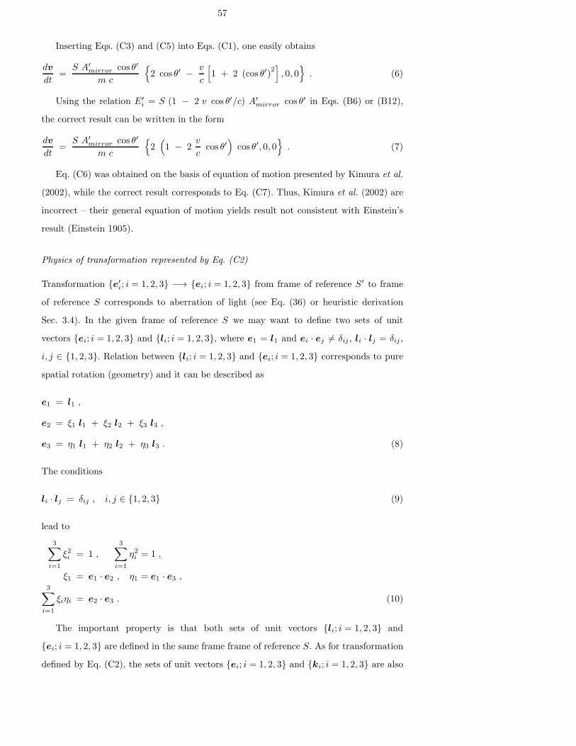
57

Inserting Eqs. (C3) and (C5) into Eqs. (C1), one easily obtains

dv

dt=

S A′mirror cos θ′

m c

2 cos θ′ − v

c

[

1 + 2 (cos θ′)2]

, 0, 0

. (6)

Using the relation E′i = S (1 − 2 v cos θ′/c) A′

mirror cos θ′ in Eqs. (B6) or (B12),

the correct result can be written in the form

dv

dt=

S A′mirror cos θ′

m c

2(

1 − 2v

ccos θ′

)

cos θ′, 0, 0

. (7)

Eq. (C6) was obtained on the basis of equation of motion presented by Kimura et al.

(2002), while the correct result corresponds to Eq. (C7). Thus, Kimura et al. (2002) are

incorrect – their general equation of motion yields result not consistent with Einstein’s

result (Einstein 1905).

Physics of transformation represented by Eq. (C2)

Transformation e′i; i = 1, 2, 3 −→ ei; i = 1, 2, 3 from frame of reference S′ to frame

of reference S corresponds to aberration of light (see Eq. (36) or heuristic derivation

Sec. 3.4). In the given frame of reference S we may want to define two sets of unit

vectors ei; i = 1, 2, 3 and li; i = 1, 2, 3, where e1 = l1 and ei · ej 6= δij , li · lj = δij ,

i, j ∈ 1, 2, 3. Relation between li; i = 1, 2, 3 and ei; i = 1, 2, 3 corresponds to pure

spatial rotation (geometry) and it can be described as

e1 = l1 ,

e2 = ξ1 l1 + ξ2 l2 + ξ3 l3 ,

e3 = η1 l1 + η2 l2 + η3 l3 . (8)

The conditions

li · lj = δij , i, j ∈ 1, 2, 3 (9)

lead to

3∑

i=1

ξ2i = 1 ,

3∑

i=1

η2i = 1 ,

ξ1 = e1 · e2 , η1 = e1 · e3 ,3∑

i=1

ξiηi = e2 · e3 . (10)

The important property is that both sets of unit vectors li; i = 1, 2, 3 and

ei; i = 1, 2, 3 are defined in the same frame frame of reference S. As for transformation

defined by Eq. (C2), the sets of unit vectors ei; i = 1, 2, 3 and ki; i = 1, 2, 3 are also

58

defined in the system S. But what about translational velocity terms + v/c in Eq. (C2)?

Any velocity term + v/c in transformation corresponds to transformation from one (lo-

cal) inertial frame of reference to another one. Thus, the conclusion is evident: Eq. (C2)

is of no physical sense.

References

Balek V., Klacka J., 2002. Perihelion motion due to the Poynting-Robertson effect.

http://xxx.lanl.gov/abs/astro-ph/0207496 (complete and different derivation: to be

submitted to General Relativity and Gravitation)

Breiter S., Jackson A. A., 1998. Unified analytical solutions to two-body problems with

drag. Mon. Not. R. Astron. Soc. 299, 237-243.

Brouwer D., Clemence G. M., 1961. Celestial Mechanics. Academic Press, New York and

London, 598 pp.

Burns J. A., Lamy P. L., Soter S., 1979. Radiation forces on small particles in the Solar

System. Icarus 40, 1-48.

Einstein A., 1905. Zur Elektrodynamik der bewegter Korper. Annalen der Physik 17,

891-920.

Gajdosık M., Klacka J., 1999. Cometary dust trails and ejection velocities. In: Evolution

and Source Regions of Asteroids and Comets, Proc. IAU Coll. 173, J. Svoren, E. M.

Pittich, and H. Rickman (eds.), Astron. Inst. Slovak Acad. Sci., Tatranska Lomnica,

pp. 239-242.

Harwit M., 1963. Origins of the Zodiacal dust cloud. J. Geophys. Res. 86, 2171-2180.

Harwit M., 1988. Astrophysical Concepts, 2-nd edition. Springer-Verlag, New York-

Berlin-Heidelberg.

Kimura H., Okamoto H., Mukai T., 2002. Radiation Pressure and the Poynting-Robertson

Effect for Fluffy Dust Particles. Icarus 157, 349-361.

Klacka J., 1992a. Poynting-Robertson effect. I. Equation of motion. Earth, Moon, and

Planets 59, 41-59.

Klacka J., 1992b. Poynting-Robertson effect. II. Perturbation equations. Earth, Moon,

and Planets 59, 211-218.

Klacka J., 1994a. Interplanetary dust particles and solar radiation. Earth, Moon, and

Planets 64, 125-132.

Klacka J., 1994b. Radial forces and orbital elements. In: Dynamics and Astrometry of

Natural and Artificial Celestial Bodies, K. Kurzynska, F. Barlier, P. K. Seidelmann

59

and I. Wytrzyszczak (eds.), Astronomical Observatory of A. Mickiewicz University,

Poznan, pp. 181-185.

Klacka J., 2000a. Electromagnetic radiation and motion of real particle.

http://xxx.lanl.gov/abs/astro-ph/0008510

Klacka J., 2000b. Aberration of light and motion of real particle.

http://xxx.lanl.gov/abs/astro-ph/0009108

Klacka J., 2000c. Solar radiation and asteroidal motion, http://xxx.lanl.gov/abs/astro-

ph/0009109

Klacka J., 2001. On the Poynting-Robertson effect and analytical solutions. In: Dynamics

of Natural and Artificial Celestial Bodies, H. Pretka-Ziomek, E. Wnuk, P. K. Seidel-

mann and D. Richardson (eds.), Kluwer Academic Publishers, Dordrecht, pp. 215-217.

(astro-ph/0004181)

Klacka J., Kaufmannova J., 1992. Poynting-Robertson effect: ‘circular’ orbit. Earth,

Moon, and Planets 59, 97-102.

Klacka J., Kaufmannova J., 1993. Poynting-Robertson effect and small eccentric orbits.

Earth, Moon, and Planets 63, 271-274.

Klacka J., Kocifaj M. 1994. Electromagnetic radiation and equation of motion for a dust

particle. In: Dynamics and Astrometry of Natural and Artificial Celestial Bodies, K.

Kurzynska, F. Barlier, P. K. Seidelmann and I. Wytrzyszczak (eds.), Astronomical

Observatory of A. Mickiewicz University, Poznan, Poland, 187-190.

Klacka J., Kocifaj M., 2001. Motion of nonspherical dust particle under the action of

electromagnetic radiation, J. Quant. Spectrosc. Radiat. Transfer 70/4-6, 595-610.

Klacka J., Saniga M., 1993. Interplanetary dust particles and solar wind. Earth, Moon,

and Planets 60, 23-29.

Kocifaj M., Klacka J., Kundracık F., 2000. Motion of realistically shaped cosmic dust

particle in Solar System. In: Light Scattering by Nonspherical Particles: Halifax Con-

tributions, G. Videen, Q. Fu, and P. Chylek (eds.), Army Research Laboratory, Adelphi

Maryland, pp. 257-261.

Landau L. D., Lifshitz E. M., 1975. The Classical Theory of Fields, 4th ed., Pergamon

Press, New York (In Russian: Teoria polia. Nauka, Moscow, 1973).

Leinert Ch., Grun E., 1990. Interplanetary dust. In: Physics of the Inner Heliosphere I,

R. Schwenn and E. Marsch (eds.), Springer-Verlag, Berlin Heidelberg, pp. 207-275.

Lyttleton R. A., 1976. Effects of solar radiation on the orbits of small particles. Astro-

physics and Space Science 44, 119-140.

60

Mediavilla E., Buitrago J., 1989. The Poynting-Robertson effect and its generalization to

the case of an extended source in rotation. Eur. J. Phys. 10, 127-132.

Mignard F., 1992. On the radiation forces. In: Interrelations Between Physics and Dy-

namics for Minor Bodies in the Solar System, D. Benest and C. Froeschle (eds.),

Frontieres, pp. 419-451.

Mishchenko M., 2001. Radiation force caused by scattering, absorption, and emission of

light by nonspherical particles. J. Quant. Spectrosc. Radiat. Transfer 70, 811-816.

Mishchenko M., Travis L. D., Lacis A. A., 2002. Scattering, Absorption and Emission of

Light by Small Particles. Cambridge University Press, Cambridge (UK), 445 pp.

Poynting J. M., 1904. Radiation in the Solar System: Its effect on temperature and its

pressure on small bodies. Philosophical Transactions of the Royal Society of London

Series A 202, 525-552.

Robertson H. P., 1937. Dynamical effects of radiation in the Solar System. Mon. Not. R.

Astron. Soc. 97, 423-438.

Robertson H. P., Noonan T. W., 1968. Relativity and Cosmology. Saunders, Philadelphia.

Srikanth, 1999. Physical interpretation of the Poynting-Robertson effect. Icarus 140, 231-

234.

Stix M., 2002. The Sun. Springer-Verlag, Berlin Heidelberg, 490 pp.

Williams I. P., 2002. The effect of radiation on the motion of meteoroids. In: Optics of

Cosmic Dust, G. Videen and M. Kocifaj (eds.), Kluwer Academic Publishers, Dor-

drecht, pp. 283-300.

Wyatt S. P., Whipple F. L., 1950. The Poynting-Robertson effect on meteor orbits. As-

trophys. J. 111, 558-565.

This article was processed by the author using Springer-Verlag LATEX A&A style file 1990.