arX

iv:a

stro

-ph/

9709

010v

2 9

Jan

199

8

Evolution of structure in cold dark matter

universes.

A. Jenkins1, C. S. Frenk1, F. R. Pearce12, P. A. Thomas2, J. M. Colberg3, S. D. M. White3,

H. M. P. Couchman4, J. A. Peacock5, G. Efstathiou67 and A. H. Nelson8

(The Virgo Consortium)

1Dept Physics, South Road, University of Durham, DH1 3LE

2CPES, University of Sussex, Falmer, Brighton BN1 9QH

3Max-Planck Inst. for Astrophysics, Garching, Munich, D-85740, Germany

4Dept of Astronomy, University of Western Ontario, London, Ontario N6A 3K7, Canada

5Royal observatory, Blackford Hill, Edinburgh, EH9 3HJ

6Dept Physics, Nuclear Physics Building, Keble Road, Oxford, OX1 3RH

7Institute of Astronomy, Madingley Road, Cambridge, CB3 OHA

8Dept of Physics and Astronomy, University of Wales, PO Box 913, Cardiff CF2 3YB

– 2 –

ABSTRACT

We present an analysis of the clustering evolution of dark matter in four cold dark

matter (CDM) cosmologies. We use a suite of high resolution, 17-million particle,

N-body simulations which sample volumes large enough to give clustering statistics

with unprecedented accuracy. We investigate a flat model with Ω0 = 0.3, an open

model also with Ω0 = 0.3, and two models with Ω = 1, one with the standard CDM

power spectrum and the other with the same power spectrum as the Ω0 = 0.3 models.

In all cases, the amplitude of primordial fluctuations is set so that the models reproduce

the observed abundance of rich galaxy clusters by the present day. We compute mass

two-point correlation functions and power spectra over three orders of magnitude in

spatial scale and find that in all our simulations they differ significantly from those of

the observed galaxy distribution, in both shape and amplitude. Thus, for any of these

models to provide an acceptable representation of reality, the distribution of galaxies

must be biased relative to the mass in a non-trivial, scale-dependent, fashion. In the

Ω = 1 models the required bias is always greater than unity, but in the Ω0 = 0.3 models

an “antibias” is required on scales smaller than ∼ 5h−1Mpc. The mass correlation

functions in the simulations are well fit by recently published analytic models. The

velocity fields are remarkably similar in all the models, whether they be characterised

as bulk flows, single-particle or pairwise velocity dispersions. This similarity is a direct

consequence of our adopted normalisation and runs contrary to the common belief that

the amplitude of the observed galaxy velocity fields can be used to constrain the value

of Ω0. The small-scale pairwise velocity dispersion of the dark matter is somewhat

larger than recent determinations from galaxy redshift surveys, but the bulk flows

predicted by our models are broadly in agreement with most available data.

– 3 –

Subject headings: cosmology: theory — dark matter — gravitation — large-scale

structure of universe

1. Introduction

Cosmological N-body simulations play a pivotal role in the study of the formation of cosmic

structure. In this methodology, initial conditions are set at some early epoch by using linear

theory to calculate the statistical properties of the fluctuations. Such a calculation requires some

specific mechanism for generating primordial structure, together with assumptions about the

global cosmological parameters and the nature of the dominant dark matter component. N-body

simulations are then used to follow the later evolution of the dark matter into the nonlinear regime

where it can be compared with the large-scale structure in galaxy surveys. This general picture

was developed fully in the early 1980s, building upon then novel concepts like the inflationary

model of the early universe and the proposition that the dark matter is non-baryonic. In the

broadest sense, it was confirmed in the early 1990s with the discovery of fluctuations in the

temperature of the microwave background radiation (Smoot et al. 1992). The plausibility of the

hypothesis that the dark matter is non-baryonic has strengthened in recent years, as the gap

between the upper limit on the density of baryons from Big Bang nucleosynthesis considerations

(e.g. Tytler et al. 1996) and the lower limit on the total mass density from dynamical studies

(e.g. Carlberg et al. 1997) has become more firmly established.

Cosmological N-body simulations were first employed to study the large-scale evolution of dark

matter on mildly nonlinear scales, a regime which can be accurately calculated using relatively few

particles. Highlights of these early simulations include the demonstration of the general principles

of nonlinear gravitational clustering (Gott, Aarseth & Turner 1979); evidence that scale-free initial

conditions evolve in a self-similar way (Efstathiou & Eastwood 1981; Efstathiou et al. 1985), while

truncated power spectra develop large-scale pancakes and filaments (Klypin & Shandarin 1983;

Centrella & Melott 1983; Frenk, White & Davis 1983); and the rejection of the proposal that

the dark matter consists of light massive neutrinos (White, Frenk & Davis 1983; White, Davis &

Frenk 1984).

During the mid-1980s, N-body simulations were extensively used to explore the hypothesis,

first elaborated by Peebles (1982), that the dark matter consists of cold collisionless particles. This

hypothesis – the cold dark matter (CDM) cosmology – has survived the test of time and remains

the basic framework for most contemporary cosmological work. The clustering evolution of dark

matter in a CDM universe was first studied in detail using relatively small N-body simulations

(Davis et al. 1985, hereafter DEFW; Frenk et al. 1985, 1988, 1990; White et al. 1987a, 1987b; Fry

& Melott 1985). In particular, DEFW concluded, on the basis of 32768-particle simulations, that

the simplest (or standard) version of the theory in which the mean cosmological density parameter

– 4 –

Ω = 1, and the galaxies share the same statistical distribution as the dark matter, was inconsistent

with the low estimates of the rms pairwise peculiar velocities of galaxies which had been obtained

at the time from the CfA redshift survey (Davis & Peebles 1983). They showed that much better

agreement with the clustering data available at the time could be obtained in an Ω = 1 CDM

model if the galaxies were assumed to be biased tracers of the mass, as in the “high peak model”

of galaxy formation (Kaiser 1984; Bardeen et al. 1986). They found that an equally successful

CDM model could be obtained if galaxies traced the mass but Ω0 ≃ 0.2, and the geometry was

either open or flat. Many of the results of this first generation of N-body simulations have been

reviewed by Frenk (1991).

Following the general acceptance of cosmological simulations as a useful technique, the

subject expanded very rapidly. To mention but a few examples in the general area of gravitational

clustering, further simulations have re-examined the statistics of the large-scale distribution

of cold dark matter (e.g. Park 1991; Gelb & Bertschinger 1994a, 1994b; Klypin, Primack &

Holtzman 1996; Cole et al. 1997;Zurek et al. 1994), confirming on the whole, the results of the

earlier, smaller calculations. Large simulations have been used to construct “mock” versions of

real galaxy surveys (e.g. White et al. 1987b; Park et al. 1994; Moore et al. 1994), or to carry

out “controlled experiments” designed to investigate specific effects such as non-gaussian initial

conditions (Weinberg & Cole 1992) or features in the power spectrum (Melott & Shandarin

1993). Some attempts have been made to address directly the issue of where galaxies form by

modelling the evolution of cooling gas gravitationally coupled to the dark matter (e.g. Carlberg,

Couchman & Thomas 1990; Cen & Ostriker 1992, Katz, Hernquist & Weinberg 1992; Evrard,

Summers & Davis 1994; Jenkins et al. 1997). The success of the N-body approach has stimulated

the development of analytic approximations to describe the weakly nonlinear behavior, using, for

example, second order perturbation theory (e.g. Bernardeau 1994; Bouchet et al. 1995), as well

as Lagrangian approximations to the fully nonlinear regime (Hamilton et al. 1991; Jain, Mo &

White 1995; Baugh & Gaztanaga 1996; Peacock & Dodds 1994, 1996; Padmanabhan 1996).

Steady progress has also been achieved on the observational front with the completion of

ever larger galaxy surveys. The first real indication that the galaxy distribution on large scales

differs from that predicted by the standard cold dark matter model was furnished by the APM

survey which provided projected positions and magnitudes for over a million galaxies. The angular

correlation function of this survey has an amplitude that exceeds the theoretical predictions by

a factor of about 3 on scales of 20 to 30h−1Mpc (Maddox et al. 1990). This result has been

repeatedly confirmed in redshift surveys of IRAS (e.g. Efstathiou et al. 1990; Saunders et al.

1990; Tadros & Efstathiou 1995), and optical galaxies (e.g. Vogeley et al. 1992; Tadros &

Efstathiou 1996; Tucker et al. 1997; Ratcliffe et al. 1997.) Modern redshift surveys have also

allowed better estimates of the peculiar velocity field of galaxies in the local universe. The original

measurement of the pairwise velocity dispersion (which helped motivate the concept of biased

galaxy formation in the first place) has been revised upwards by Mo, Jing and Borner (1993) and

Sommerville, Davis & Primack (1997), but Marzke et al. (1995) and Mo, Jing & Borner (1996)

– 5 –

have argued that such pairwise statistics are not robust when determined from relatively small

redshift surveys. The Las Campanas redshift survey is, perhaps, the first which is large enough to

give a robust estimate of these statistics (Jing, Mo & Borner 1997). Surveys of galaxy distances

are also now beginning to map the local mean flow field of galaxies out to large distances (e.g.

Lynden-Bell et al. 1988; Courteau et al. 1993; Mould et al. 1993; Dekel et al. 1997; Giovanelli

1997; Saglia et al. 1997; Willick et al. 1997.) Both pairwise velocity dispersions and mean flows

allow an estimate of the parameter combination β ≡ Ω0.60 /b (where b is the biasing parameter

defined in Section 5); recent analyses seem to be converging on values of β around 0.5.

In this paper we present results from a suite of very large, high-resolution N-body simulations.

Our primary aim is to extend the N-body work of the 1980s and early 1990s by increasing

the dynamic range of the simulations and calculating the low-order clustering statistics of the

dark matter distribution to much higher accuracy than is possible with smaller calculations.

Our simulations follow nearly 17 million particles, with a spatial resolution of a few tens of

kiloparsecs and thus probe the strong clustering regime whilst correctly including large-scale

effects. Such improved theoretical predictions are a necessary counterpart to the high precision

attainable with the largest galaxy datasets like the APM survey and particularly the forthcoming

generation of redshift surveys, the Sloan (Gunn & Weinberg 1995) and 2-degree field (http:\\www.ast.cam.ac.uk\ 2dFgg\) projects. Our simulations do not address the issue of where galaxies

form. They do, however, reveal in quantitative detail the kind of biases that must be imprinted

during the galaxy formation process if any of the models is to provide an acceptable match to the

galaxy clustering data. We examine four versions of the cold dark matter theory including, for the

first time, the τCDM model. This has Ω = 1 but more power on large scales than the standard

version and offers an attractive alternative to the standard model if Ω = 1. We focus on high

precision determinations of the spatial and velocity distributions and also carry out a comparison

of the simulation results with the predictions of analytic clustering models.

Many of the issues we discuss in this paper have been addressed previously using large N-body

simulations. Our study complements and supersedes aspects of this earlier work because our

simulations are significantly larger and generally have better resolution than earlier simulations

and also because we investigate four competing cosmological models in a uniform manner. Thus,

for example, Gelb and Bertschinger (1994b) studied the standard Ω = 1 CDM model but most of

their simulations had significantly poorer spatial resolution than ours and the one with similar

resolution had only 1% of the volume. Klypin et al. (1996) simulated a low-Ω0 flat CDM model

with a mass resolution at least 10 times poorer than ours or in volumes that were too small to

properly include the effects of rare objects. These simulations missed a number of subtle, but

nevertheless important, effects that are revealed by our larger simulations. Our analysis has

some features in common with the recent work of Cole et al. (1997) who simulated a large suite

of cosmologies in volumes that are typically three times larger than ours, but have 3-6 times

fewer particles and an effective mass resolution an order of magnitude less than ours. Their force

resolution is also a factor of three times worse that ours. While Cole et al. focussed on models

– 6 –

in which the primordial fluctuation amplitude is normalised using the inferred amplitude of the

COBE microwave background fluctuations, our models are normalized so that they all give the

observed abundance of rich galaxy clusters by the present day. Our choice of normalisation is

motivated and explained in Section 3.

This study is part of the programme of the “Virgo consortium,” an international collaboration

recently constituted with the aim of carrying out large N-body and N-body/gasdynamic

simulations of large-scale structure and galaxy formation, using parallel supercomputers in

Germany and the UK. Some of our preliminary results are discussed in Jenkins et al. (1997) and

further analysis of the present simulations may be found in Thomas et al. (1997).

The cosmological parameters of our models are described in Section 2 and their numerical

details in Section 3. Colour images illustrating the evolution of clustering in our simulations are

presented in Section 4. The evolution of the mass correlation functions and power spectra are

discussed, and compared with observations, in Sections 5 and 6. We compare these clustering

statistics with analytic models for the nonlinear evolution of correlation functions and power

spectra in Section 7. The present day velocity fields, both bulk flows and pairwise dispersions,

are discussed in Section 8. Our paper concludes in Section 9 with a discussion and summary

(including a table) of our main results.

2. Cosmological models

We have simulated evolution in four CDM cosmologies with parameters suggested by a variety

of recent observations. The shape of the CDM power spectrum is determined by the parameter,

Γ, (c.f. equation 4 below); observations of galaxy clustering, interpreted via the assumption that

galaxies trace the mass, indicate a value Γ ≃ 0.2 (Maddox et al. 1990, 1996; Vogeley et al. 1992).

In the standard version of the theory, Γ = Ω0h,1 which corresponds, for low baryon density, to

the standard assumption that only photons and three massless species of neutrinos and their

antiparticles contribute to the relativistic energy density of the Universe at late times. For a given

Ω and h, smaller values of Γ are possible, but this requires additional physics, such as late decay

of the (massive) τ -neutrino to produce an additional suprathermal background of relativistic e-

and µ-neutrinos at the present day (White, Gelmini & Silk 1995). This has the effect of delaying

the onset of matter domination, leading to a decrease in the effective value of Γ.

In addition to observations of large-scale structure, a second consideration that has guided

our choice of cosmological models is the growing evidence in favour of a value of Ω0 around 0.3.

The strongest argument for this is the comparison of the baryon fraction in rich clusters with the

universal value required by Big Bang nucleosynthesis (White et al. 1993; White & Fabian 1995;

Evrard 1997). The recently determined abundance of hot X-ray emitting clusters at z ≃ 0.3 also

1Here and below we denote Hubble’s constant H0 by h = H0/100 kms−1Mpc−1

– 7 –

indicates a similar value of Ω0 (Henry 1997.) The strength of these tests lies in the fact that they

do not depend on uncertain assumptions regarding galaxy formation. Nevertheless, they remain

controversial and so, in addition to cosmologies with Ω0 = 0.3, we have also simulated models with

Ω = 1.

Three of our simulations have a power spectrum shape parameter, Γ = 0.21. One of these

(ΛCDM) has Ω0 = 0.3 and the flat geometry required by standard models of inflation, i.e.

λ ≡ Λ/(3H2) = 0.7 (where Λ is the cosmological constant and H is Hubble’s constant). The

second model (OCDM) also has Ω0 = 0.3, but Λ = 0. In both these models we take h = 0.7,

consistent with a number of recent determinations (Kennicutt, Freedman & Mould 1995). Our

third model with Γ = 0.21 (τCDM) has Ω = 1 and h = 0.5; this could correspond to the decaying

neutrino model mentioned above. Finally, our fourth model is standard CDM (SCDM) which has

Ω = 1, h = 0.5, and Γ = 0.5. Thus, two of our models (ΛCDM and OCDM) differ only in the value

of the cosmological constant; two others (ΛCDM and τCDM) have the same power spectrum and

geometry but different values of Ω0; and two more (τCDM and SCDM) differ only in the shape of

the power spectrum.

Having chosen the cosmological parameters, we must now set the amplitude of the initial

fluctuation spectrum. DEFW did this by requiring that the slope of the present day two-point

galaxy correlation function in the simulations should match observations. This was a rather

crude method, but one of the few practical alternatives with the data available at the time. The

discovery of fluctuations in the temperature of the microwave background radiation by COBE

offered the possibility of normalising the mass fluctuations directly by relating these to the

measured temperature fluctuations on large scales. In practice, however, the large extrapolation

required to predict the amplitude of fluctuations on scales relevant to galaxy clustering from

the COBE data makes this procedure unreliable because it depends sensitively on an uncertain

assumption about the slope of the primordial power spectrum. A further source of uncertainty is

the unknown contribution to the COBE signal from tensor (rather than scalar) modes. In spite

of these uncertainties, it is remarkable that the normalisation inferred from the simplest possible

interpretation of the COBE data is within about a factor of 2 of the normalisation inferred for

standard CDM by DEFW from galaxy clustering considerations.

A more satisfactory procedure for fixing the amplitude of the initial mass fluctuations is to

require that the models should match the observed abundance of galaxy clusters. The distribution

of cluster abundance, characterised by mass, X-ray temperature or some other property, declines

exponentially and so is very sensitive to the normalisation of the power spectrum (Frenk et

al. 1990). Using the observed cluster abundance to normalise the power spectrum has several

advantages. Firstly, it is based on data which are well matched to the scales of interest; secondly,

it gives the value of σ8 (the linearly extrapolated rms of the density field in spheres of radius

8h−1Mpc) with only a weak dependence on the shape of the power spectrum if Ω < 1 and

no dependence at all if Ω = 1 (White, Efstathiou & Frenk 1993); thirdly, it does not require

a particularly accurate estimate of the abundance of clusters because of the strong sensitivity

– 8 –

of abundance on σ8. The disadvantage of this method is that it is sensitive to systematic

biases arising from inaccurate determinations of the particular property used to characterize the

abundance. However, the consistency of the estimates of σ8 when the abundance of clusters is

characterized by total mass (Henry & Arnaud 1991), by mass within the Abell radius (White,

Efstathiou & Frenk 1993), or by the X-ray temperature of the intracluster medium (Eke, Cole &

Frenk 1996; Viana & Liddle 1996) suggests that systematic effects are likely to be small.

We adopt the values of σ8 recommended by Eke, Cole & Frenk (1996) from their analysis of

the local cluster X-ray temperature function. This requires:

σ8 = (0.52 ± 0.04)Ω−0.52+0.13Ω0

0 (flat models) (1)

or

σ8 = (0.52 ± 0.04)Ω−0.46+0.1Ω0

0 (open models) (2)

These values of σ8 are consistent with those obtained from the slightly different analyses carried

out by White, Efstathiou & Frenk (1993), Viana & Liddle (1996) and Henry (1997).

The resulting values of σ8 for our simulations are listed in Table 1. For reference, these

values may be compared to those required by the COBE data under the simplest set of

assumptions, namely that the primordial power spectrum is a power-law with exponent n = 1 (the

Harrison-Zel’dovich spectrum) and that there is no contribution at all from tensor modes. For

our chosen cosmologies, the 4-year COBE-DMR data imply values of σ8 of 1.21, 0.45, 1.07, 0.52

(Gorski et al. 1995, Ratra et al. 1997) for SCDM, τCDM, ΛCDM, and OCDM respectively. Thus,

our τCDM and ΛCDM models are roughly consistent with the conventional COBE normalisation,

but our adopted normalisations for the SCDM and OCDM models are ∼ 40% lower and ∼ 60%

higher respectively than the COBE values. These numbers are consistent with those obtained

by Cole et al. (1997) from their grid of large COBE-normalised cosmological N-body simulations

with different parameter values. As may be seen from their Figure 4, there is only a small

region of parameter space in which the conventional COBE-normalised CDM models produce the

correct abundance of clusters. Flat models require 0.25 ≤ Ω0 ≤ 0.4 while open models require

0.4 ≤ Ω0 ≤ 0.5.

To summarize, we have chosen to simulate four cosmological models which are of interest

for a variety of reasons. Our three flat models are consistent with standard inflationary theory

and our open model can be motivated by the more exotic “open bubble” version of this theory

(Garcia-Bellido & Linde 1997). By construction, all our models approximately reproduce the

observed abundance of rich galaxy clusters. The ΛCDM model has a value of Ω0 in line with

recent observational trends and a value of Γ that is close to that inferred from galaxy clustering. It

has the additional advantages that its normalisation agrees approximately with the conventional

COBE normalisation and, for our adopted value of H0, it has an age that is comfortably in accord

with traditional estimates of the ages of globular clusters (Renzini et al. 1996, but see Jimenez

et al. 1996). The OCDM model shares some of these attractive features but allows us also to

investigate the effects of the cosmological constant on the dynamics of gravitational clustering.

– 9 –

Its normalisation is higher than required to match the conventional COBE value, but this could

be rectified by a modest increase in Ω0 to about 0.4-0.5. The τCDM model is as well motivated

by galaxy clustering data as are the low-Ω0 models and has the advantage that it allows us to

investigate the dynamical effects of changing Ω0 while keeping the shape of the initial power

spectrum fixed. Finally, the traditional SCDM model is an instructive counterpart to its τCDM

variant.

3. The Simulations

Our simulations were carried out using a parallel, adaptive particle-particle/particle-mesh

code developed by the Virgo consortium (Pearce et al. 1995, Pearce & Couchman 1997). This

is identical in operation to the publicly released serial version of “Hydra” (Couchman, Pearce &

Thomas 1996; see Couchman, Thomas & Pearce 1995 for a detailed description.) The simulations

presented in this paper are the first carried out by the Virgo consortium and were executed on

either 128 or 256 processors of the Cray T3Ds at the Edinburgh Parallel Computing Centre and

the Rechenzentrum, Garching.

The force calculation proceeds through several stages. Long range gravitational forces are

computed in parallel by smoothing the mass distribution onto a mesh, typically containing 5123

cells, which is then fast Fourier transformed and convolved with the appropriate Green’s function.

After an inverse FFT, the forces are interpolated from the mesh back to the particle positions.

In weakly clustered regions, short range (particle-particle) forces are also computed in parallel

using the entire processor set. Hydra recursively places additional higher resolution meshes, or

refinements, around clustered regions. Large refinements containing over ≃ 105 particles are

executed in parallel by all processors while smaller refinements, which fit within the memory of a

single processor, are most efficiently executed using a task farm approach. The parallel version

of Hydra employed in this paper is implemented in CRAFT, a directive based parallel Fortran

compiler developed for the Cray T3D supercomputer (Cray Research Inc). We have checked that

the introduction of mesh refinements in high density regions does not introduce inaccuracies in

the computation by redoing our standard τCDM simulation using a parallel P3M code (without

refinements). The two-point correlation functions in these two simulations differed by less than

0.5% over the range 0.1h−1Mpc – 5h−1Mpc.

3.1. Simulation details

Initial conditions were laid down by imposing perturbations on an initially uniform state

represented by a “glass” distribution of particles generated by the method of White (1996). Using

the algorithm described by Efstathiou et al. (1985), based on the Zel’dovich (1970) approximation,

a Gaussian random field is set up by perturbing the positions of the particles and assigning

– 10 –

them velocities according to growing mode linear theory solutions. Individual modes are assigned

random phases and the power for each mode is selected at random from an exponential distribution

with mean power corresponding to the desired power spectrum ∆2(k).

Following Peebles’ (1980) convention we define the dimensionless power spectrum, ∆2(k), as

the power per logarithmic interval in spatial frequency, k:

∆2(k) ≡ V

(2π)34π k3 |δk|2, (3)

where |δk|2 is the power density and V is the volume. If the primordial power spectrum is of the

form |δk|2 ∝ kn, then the linear power spectrum at a later epoch is given by ∆2(k) = kn+3T 2(k, t),

where T (k, t) is the transfer function. The standard inflationary model of the early universe

predicts that n ≃ 1 (Guth & Pi 1982) and we shall take n = 1. For a cold dark matter model,

the transfer function depends on the values of h and the mean baryon density Ωb. We use the

approximation to the linear CDM power spectrum given by Bond & Efstathiou (1984),

∆2(k) =Ak4

[

1 + [aq + (bq)3/2 + (cq)2]ν]2/ν

, (4)

where q = k/Γ, a = 6.4h−1Mpc, b = 3h−1Mpc, c = 1.7h−1Mpc and ν = 1.13. The normalisation

constant, A, is chosen by fixing the value of σ8 as discussed in Section 2.

For our models, the analytic approximation of equation (4) provides a good approximation

to the accurate numerical power spectrum calculated by Seljak & Zaldarriaga (1996) using

their publicly available code CMBFAST (http://arcturus.mit.edu:80/ ∼matiasz/ CMBFAST

/cmbfast.html). For example, setting h = 0.7 and Ωb = 0.026 in our ΛCDM and OCDM and

normalizing to the same value of σ8, we find that the maximum difference at small scales between

the fit of equation (4) and the output of CMBFAST is 13% in power or 6% in amplitude. These

numbers are smaller for a lower value of Ωb or a small increase in h. These differences are

comparable to those induced by plausible changes in Ωb or h. (For example, for a ΛCDM model,

the ratio of the σ8-normalized CMBFAST power spectra for Ωb = 0.01 and Ωb = 0.03 respectively

is 1.08 at the Nyquist frequency of our simulation volumes (k = 3.36hMpc−1) and 0.85 at the

fundamental frequency (k = 0.0262hMpc−1); if Ωb is kept fixed but h is allowed to vary between

0.67 and 0.73, these ratios become 1.08 and 0.9 respectively.) Similarly, we set up our τCDM

model simply by changing the value of Γ in equation (4). This gives a satifactory fit provided that

the length-scale introduced in the power spectrum by the decay of the τ -neutrino is smaller than

Nyquist frequency of the simulation volume. This requires the mass of the decaying particle to be

in excess of about 10keV (Bond & Efstathiou 1991). Thus, over the range of wavenumbers relevant

to our simulations, equation (4) gives a good, but not perfect approximation to the true τCDM

power spectrum for a broad one-dimensional subset of the two-dimensional mass-lifetime space for

the τ -neutrino (see White et al 1995). Again, these diferences are small compared to those induced

by changes, similar to above, in Ωb and h. Finally, as discussed above, the normalisation of the

– 11 –

power spectrum from the cluster abundance is uncertain by at least 15% (1-σ) (Eke, Cole & Frenk

1996). These various uncertainties limit the accuracy with which the dark matter distribution can

be calculated at the present time.

For each cosmological model we analyse two simulations of regions of differing size. To

facilitate intercomparison, we employed the same random number sequence to generate initial

conditions for all these simulations. To test for finite volume effects, however, we carried out an

additional simulation of the τCDM model, this time using a different realisation of the initial

conditions. In the first set of simulations (which includes the extra τCDM model), we adopted

a box length L = 239.5h−1Mpc. The gravitational softening length was initially set to 0.3 times

the grid spacing and was kept constant in comoving coordinates until it reached the value given

in Table 1, at z ≃ 3. Thereafter, it was kept constant in physical units. (The functional form

of the gravitational softening used is that given by Efstathiou & Eastwood 1981; the values we

quote correspond to the softening scale of a Plummer potential which matches the actual force law

asymptotically at both large and small scales. The actual force is 53.6% of the full 1/r2 force at

one softening length and more than 99% at two softening lengths.) In the second set of simulations,

the particle mass in solar masses (rather than the volume) was kept constant in all four models

and the gravitational softening was taken to be either 30h−1kpc or 36h−1kpc in physical units

(after initially being kept fixed in comoving coordinates as before). The mass resolution in these

simulations is a factor of 3-20 better than in the first set. The large box simulations are large

enough to give unbiased results and relatively small sampling fluctuations for all the statistics we

study, with the exception of large-scale bulk flows. For example, on scales < 5h−1Mpc the typical

differences in the correlation function and pair-wise velocities of the two τCDM realisations are

only about 2%. We use the large box simulations for most of our analysis of large-scale clustering

and velocities (Sections 5, 6, 8). The smaller volume simulations, on the other hand, resolve

structures down to smaller mass scales. We use these to test the effects of numerical resolution and

for a comparison with analytic models in Section 7, where special emphasis is given to the strong

clustering regime. All our simulations have 16.7 million particles. The number of timesteps varied

between 613 and 1588. The SCDM and τCDM simulations were started at z = 50; the OCDM at

z = 119 and the ΛCDM at z = 30. The parameters of our simulations are listed in Table 1.

4. Slices through the simulations

Figures 1, 2, 3 (colour plates 1, 2, and 3) show slices through the dark matter distribution in

our four models at three different redshifts: z = 0, 1, and 3. The slices are 239.5h−1Mpc on a side

and have thickness a tenth of the side length. The projected mass distribution in these slices was

smoothed adaptively onto a fine grid employing a variable kernel technique similar to that used to

estimate gas densities in Smoothed Particle Hydrodynamics.

– 12 –

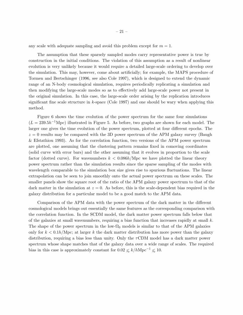
Fig. 1.— The projected mass distribution at z = 0 in slices through four CDM N-body simulations.

The length of each slice is 239.5h−1Mpc and the thickness is one tenth of this. To plot these slices,

the mass distribution was first smoothed adaptively onto a fine grid using a variable kernel technique

similar to that used to estimate gas densities in Smoothed Particle Hydrodynamics. At z = 0, the

general appearance of all the models is similar because, by construction, the phases of the initial

fluctuations are the same. On larger scales, the higher fluctuation amplitude in the ΛCDM and

OCDM models is manifest in sharper filaments and larger voids compared to the SCDM and τCDM

models. The two Ω = 1 models look very similar as do the two Ω0 = 0.3 models but, because of

their higher normalisation, the latter show more structure.

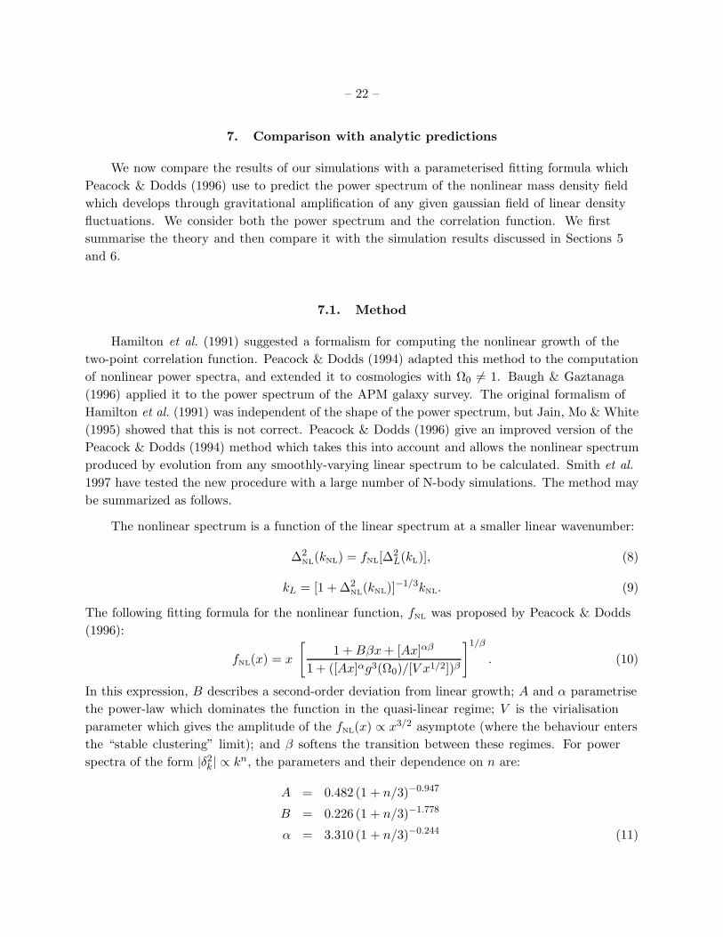
Fig. 2.— The projected mass distribution at z = 1 in slices through four CDM N-body simulations.

The slices show the same region as Figure 1. The large-scale differences amongst the models are

much more apparent at z = 1 than at z = 0 because of the different rates at which structure grows

in these models. The linear growth factor relative to the present value is 0.5 for SCDM and τCDM,

0.61 for ΛCDM, and 0.68 for OCDM.

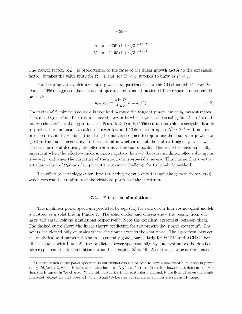
Fig. 3.— The projected mass distribution at z = 3 in slices through four CDM N-body simulations.

The slices show the same region as Figures 1 and 2. At this early epoch the differences amongst

the models are even more striking than at z = 1 (c.f. Figure 2.) The linear growth factor relative

to the present value is 0.25 for SCDM and τCDM, 0.32 for ΛCDM, and 0.41 for OCDM.

– 13 –

At z = 0, the general appearance of all the models is similar because, by construction,

the phases of the initial fluctuations are the same. The now familiar pattern of interconnected

large-scale filaments and voids is clearly apparent. However, at the high resolution of these

simulations, individual galactic dark halos are also visible as dense clumps of a few particles. On

larger scales, the higher fluctuation amplitude in the ΛCDM and OCDM models is manifest in

sharper filaments and larger voids compared to the SCDM and τCDM models. Because of their

higher normalisation, the low Ω0 models also have more small-scale power than SCDM and τCDM

and this results in tighter virialized clumps. The linearly evolved power spectra of ΛCDM and

OCDM are almost identical and so the primary differences between them reflect their late time

dynamics, dominated by the cosmological constant in one case, and by curvature in the other. In

OCDM, structures of a given mass collapse earlier and so are more compact than in ΛCDM. The

fine structure in SCDM and τCDM is similar but since the relative amounts of power in these

models cross over at intermediate scales, clumps are slightly fuzzier in the τCDM case.

The large-scale differences amongst the models are much more apparent at z = 1. There is

substantially more evolution for Ω = 1 than for low-Ω0; in the former case, the linear growth

factor is 0.50 of the present value, whereas in ΛCDM and OCDM it is 0.61 and 0.68 respectively.

Thus, OCDM has the most developed large-scale structure at z = 1, while ΛCDM is intermediate

between this and the two Ω = 1 models. By z = 1, the OCDM model has already become

curvature dominated (Ω = 0.46) but the cosmological constant is still relatively unimportant in

the ΛCDM model (Ω = 0.77).

At the earliest epoch shown, z = 3, the differences between the models are even more striking.

The linear growth factor for SCDM and τCDM is 0.25 while for ΛCDM it is 0.32 and for OCDM

0.41 of its present value. The SCDM model is very smooth, with only little fine structure. The

τCDM model has some embryonic large-scale structure but it is even more featureless that SCDM

on the finest scales. By contrast, structure in the low-Ω0 models, particularly OCDM is already

well developed by z = 3.

5. The two-point correlation functions

In this section we discuss the redshift evolution of the mass two-point correlation function,

ξ(r), and compare the results at z = 0 with estimates for the observed galaxy distribution.

For each volume we have a single simulation from which to estimate ξ(r). Since this volume

is assumed to be periodic, contributions to the correlation function from long wavelength modes

are poorly sampled. In principle, it is possible to add a systematic correction, based on the linear

theory growth of long wavelength modes (see the Appendix for a derivation):

ξ(r) =∞∑

n6=(0,0,0)

−ξlin(|r + Ln|) (5)

– 14 –

where L is the simulation boxlength and ξlin is the linear theory correlation function given in

terms of the linearly evolved power spectrum ∆2lin by:

ξlin(r) =

∫ ∞

0∆2

lin

(sin kr

kr

)dk

k. (6)

This expression gives a correction which is negligible for most of our simulation volumes. For

example, for τCDM2, our simulation with the smallest box size (L = 84.5h−1Mpc) and substantial

large-scale power (Γ = 0.21), the correction is only 0.01 at small separations. The expression in

eqn (5) is approximately a factor of three smaller for the 84.5h−1Mpc volume than the heuristic

correction,∫ 2π/L0 ∆2(sin kr/kr)dk/k, used by Klypin, Primack & Holtzman (1996). In any case,

for a single simulation there is also a random error associated with the fact that the power

originally assigned to each mode is drawn from a distribution. This introduces a random scatter in

the correlation function which is comparable to the correction in eqn (5). The most direct way of

assessing the importance of this effect in our simulations is by comparing two or more realizations

of the same model. For the case of τCDM, we have carried out a second simulation with identical

parameters to the first one, but using a different random number seed to set up initial conditions.

The difference between the correlation functions of these two simulations are less than 2% on all

scales below < 5h−1Mpc, comparable to the thickness of the line used to plot them in Figure 5

below.

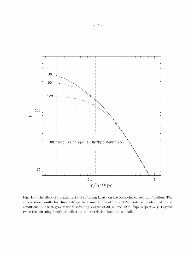
On small scales the amplitude of the two-point correlation function is suppressed by resolution

effects due to the use of softened gravity and finite mass resolution. To test the first of these

effects, we performed a series of three simulations of the τCDM model with 1283 particles, identical

initial conditions, the same mass resolution as the τCDM1a simulation, and three different values

of the gravitational softening length. The resulting two-point correlation functions are shown in

Figure 4. The effects on the correlation function at twice the softening length are very small.

Similarly, mass resolution effects in our simulations are small, as we discuss later in this Section

and in Section 7.

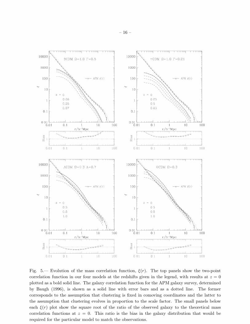
Figure 5 shows the mass two-point correlation functions in our four cosmological models

at four different epochs. These data were computed using the simulations SCDM1, τCDM1a,

ΛCDM1, and OCDM1. As the clustering grows, the amplitude of the correlation function

increases in a nonlinear fashion. The overall shape of ξ(r) is similar in all the models. In all

cases, d2ξ/dr2 < 0 on scales below r ∼ 500h−1kpc and there is an inflection point on scales of a

few megaparsecs. The flattening off of ξ(r) at small pair separations is unlikely to be a numerical

artifact. It occurs on scales that are several times larger than the gravitational softening length

and are well resolved. That this change in slope is not due to mass resolution effects (associated,

for example, with the limited dynamic range of the initial conditions) is demonstrated by the

excellent agreement between the small-scale behavior of the correlation functions plotted in

Figure 5 and the correlation functions of our smaller volume simulations which have 3-20 times

better mass resolution (c.f. Figure 8 below; see also Little, Weinberg & Park 1991 for a discussion

of why neglecting the power below the Nyquist frequency of the initial conditions has little effect

– 15 –

0.1 1

10

100

Fig. 4.— The effect of the gravitational softening length on the two-point correlation function. The

curves show results for three 1283-particle simulations of the τCDM model with identical initial

conditions, but with gravitational softening lengths of 30, 60 and 120h−1kpc respectively. Beyond

twice the softening length the effect on the correlation function is small.

– 16 –

Fig. 5.— Evolution of the mass correlation function, ξ(r). The top panels show the two-point

correlation function in our four models at the redshifts given in the legend, with results at z = 0

plotted as a bold solid line. The galaxy correlation function for the APM galaxy survey, determined

by Baugh (1996), is shown as a solid line with error bars and as a dotted line. The former

corresponds to the assumption that clustering is fixed in comoving coordinates and the latter to

the assumption that clustering evolves in proportion to the scale factor. The small panels below

each ξ(r) plot show the square root of the ratio of the observed galaxy to the theoretical mass

correlation functions at z = 0. This ratio is the bias in the galaxy distribution that would be

required for the particular model to match the observations.

– 17 –

on nonlinear evolution.) Rather, the flattening of ξ(r) at small pair separations seems to be due to

the transition into the “stable clustering” regime. We return to this point in Section 7 where we

compare the correlation functions in the simulations with analytic models for nonlinear evolution.

The mass correlation functions at z = 0 (thick solid lines) may be compared with the observed

galaxy correlation function. The largest dataset available for this comparison is the APM galaxy

survey of over 106 galaxies for which Baugh (1996) has derived the two-point correlation function,

ξg(r), by inverting the measured angular correlation function, w(θ). The advantage of this

procedure is that it gives a very accurate estimate of the correlation function in real space, but

the disadvantage is that it requires assumptions for the redshift distribution of the survey galaxies

and for the evolution of ξg(r) in the (relatively small) redshift range sampled by the survey. The

solid line with error bars in Figure 5 assumes that clustering on all scales is fixed in comoving

coordinates, whilst the dotted line assumes that clustering evolves in proportion to the scale

factor. Changes in the assumed redshift distribution produce a systematic scaling of the entire

correlation function. On scales ∼> 20 − 30h−1Mpc, the statistical error bars may underestimate

the true uncertainty in ξg(r) since residual systematic errors in the APM survey on these scales

cannot be ruled out (Maddox et al. 1996.)

None of the model mass correlation functions match the shape of the observed galaxy

correlation function. For the galaxies, ξg(r) is remarkably close to a power-law over 4 orders of

magnitude in amplitude above ξg = 1; at larger pair separations, it has a broad shoulder feature.

By contrast, the slope of the mass correlation functions in the models varies systematically, so

that none of the theoretical curves is adequately fit by a single power-law over a substantial range

of scales. We have checked (Baugh, private communication) that the inversion procedure used

to derive the APM ξg(r) from the measured w(θ) does not artificially smooth over features that

may be present in the intrinsic clustering pattern. We have also checked that features present in

the model ξ(r) are still identifiable in the corresponding w(θ) derived with the same assumptions

used in the APM analysis. The differences in shape and amplitude between the theoretical and

observed correlation functions may be conveniently expressed as a “bias function.” We define the

bias as the square root of the ratio of the observed galaxy to the theoretical mass correlation

functions at z = 0, b(r) ≡ [ξg(r)/ξ(r)]1/2, and plot this function at the bottom of each panel in

Figure 5. At each pair separation, b(r) gives the factor by which the galaxy distribution should be

biased in order for the particular model to match observations. For all the models considered here

the required bias varies with pair separation.

The standard CDM model, illustrated in the top left panel, shows the well-known shortfall

in clustering amplitude relative to the galaxy distribution on scales greater than 8h−1Mpc. The

required bias is close to unity on scales of 0.1 − 1h−1Mpc, but then rises rapidly with increasing

scale. The choice of Γ = 0.21 for the other models leads to mass correlation functions with shapes

that are closer to that of the galaxies on large scales. For these models, the slope of the bias

function is relatively modest on scales ∼> 10h−1Mpc. The large-scale behavior of b(r), however,

may be affected by possible systematic errors in the APM w(θ) at large pair separations and by

– 18 –

finite box effects in the simulations. The τCDM model, which has the smallest amount of small

scale power, requires a significant positive bias everywhere, b ≃ 1.5, and this is approximately

independent of scale from ∼ 0.2 − 10h−1Mpc. At smaller pair separations, the bias increases

rapidly. As discussed in the next section, the power spectrum, which is less affected by finite

box effects than the correlation function, indicates that a constant bias for the τCDM model is

consistent with the APM data even on scales larger than 10h−1Mpc. Thus, uniquely amongst

the models we are considering, the shape of the correlation function and power spectrum in the

τCDM model are quite similar to the observations on scales ∼> 0.2h−1Mpc.

In the ΛCDM and OCDM models, the amplitude of the dark matter ξ(r) is close to unity at

r = 5h−1Mpc, the pair separation at which ξg(r) is also close to unity. However, at small pair

separations, the mass correlation function has a much steeper slope than the galaxy correlation

function and, as result, ξ(r) rises well above the galaxy data. Thus, our low-density models

require an “antibias”, i.e. a bias less than unity, on scales ≃ 0.1 − 4h−1Mpc. A similar conclusion

was reached by Klypin, Primack & Holtzman (1996) from a lower resolution N-body simulation

of a similar ΛCDM model. As pointed out by Cole et al. (1997), the requirement that galaxies

be less clustered than the mass must be regarded as a negative feature of these models. Even if

a plausible physical process could be identified that would segregate galaxies and mass in this

manner, dynamical determinations of Ω0 from cluster mass-to-light ratios tend to give values of

Ω0 ≃ 0.2 if the galaxies are assumed to trace the mass (e.g. Carlberg et al. 1997). If, instead, the

galaxy distribution were actually antibiased, this argument would result in an overestimate of the

true value of Ω0. Models with Ω0 smaller than our adopted value of 0.3, require even larger values

of σ8, and therefore even larger antibias, in order to match the observed abundance of galaxy

clusters. In our Ω = 1 models, the required bias always remains above unity and is, in fact, quite

close to unity over a large range in scales. This is an attractive feature of these models which may

help reconcile them with virial analyses of galaxy clusters (Frenk et al. 1996), and results, in part,

from the relatively low normalisation required to match the cluster abundance. However, the bias

we infer is only about 60% of the value required by Frenk et al. (1990) to obtain acceptable cluster

mass-to-light ratios in an Ω = 1 CDM cosmology with “high peak” biasing.

It seems almost inevitable that the process of galaxy formation and subsequent dynamical

evolution will bias the galaxy distribution relative to the mass in a complicated way. Indeed, a

variety of biasing mechanisms have been discussed in the past. These are essentially of two types.

In the first, galaxy formation is assumed to be modulated, for example, by the local value of the

density smoothed on cluster scales, as in the high peak bias model of galaxy formation (Bardeen

et al. 1986; DEFW), or by the effects of a previous generation of protogalaxies (e.g. Dekel &

Rees 1987). Such local processes tend to imprint features on the galaxy correlation function on

small and intermediate scales, but Coles (1993) and Weinberg (1995) have argued that they do

not appreciably distort the shape of the mass correlation function on large scales. This, however,

may be achieved by some form of non-local bias like in the “cooperative galaxy formation” scheme

proposed by Bower et al. (1993; see also Babul & White 1991). In this case, a match to the APM

– 19 –

w(θ) on large scales is possible with a suitable choice of model parameters. The second type of

biasing mechanism is of dynamical origin. An example is the “natural bias” found in the CDM

simulations of White et al. (1987b) who showed that the dependence of fluctuation growth rate on

mean density naturally biases the distribution of massive dark halos towards high density regions

(see also Cen & Ostriker 1992.) Another example is dynamical friction which, as Richstone, Loeb

& Turner (1992) and Frenk et al. (1996) amongst others have shown, can segregate galaxies from

mass in rich clusters. Dynamical biases of this type tend to enhance the pair count at small

separations, flattening the bias function on scales of a few hundred kiloparsecs. Mergers, on the

other hand, have the opposite effect and may even give rise to an antibias of the kind required in

our low-Ω0 models (c.f. Jenkins et al. 1997). Thus, it seems likely that the correlation function of

the galaxies that would form in our models will differ from the correlation function of the mass.

Nevertheless, the fine tuning required to end up with an almost featureless power-law correlation

function over at least two orders of magnitude in scale seems a considerable challenge for this

general class of models.

6. The power spectra

For an isotropic distribution in k-space, the power spectrum is related to the correlation

function by

ξ(r) =

∫ ∞

0∆2(k)

(sin kr

kr

)dk

k. (7)

To measure the power spectrum of our simulations over a wide range of scales we use a

technique which is efficient both in terms of computational expense and memory. To evaluate the

power spectrum on the smallest scales, we divide the computational volume into m3 equal cubical

cells and superpose the particle distributions of all m3 cells. The Fourier transform of this density

distribution, which is now periodic on a scale L/m, recovers exactly the power present in the full

simulation volume in modes which are periodic on the scale L/m. These modes form a regular

grid of spacing 2mπ/L in k-space. The estimate of ∆2(r) is obtained by averaging the power of

large numbers of modes in spherical shells. Provided these modes have, on average, representative

power this gives an unbiased estimate of the power spectrum of the simulation. In principle, the

power of all the modes in the full simulation can be obtained by applying a complex weighting,

exp(2πin · r/L), to a particle at position r during the charge assignment prior to taking the

discrete fast Fourier transform. This charge assignment creates a uniform translation in k-space

by 2πn/L. With a suitable choice of n one can recover a different set of modes from the original

simulation, always with a spacing of 2mπ/L in k-space. Applying this method m3 times allows

the recovery of all modes present in the simulation, although there is no longer any gain in CPU

time over a single large fast Fourier transform. Because of the sparse sampling of k-space, the

estimate of the power on the scale L/m has a large variance. However, by using a 643 mesh and

evaluating the Fourier transform for several values of m one can evaluate the power spectrum on

– 20 –

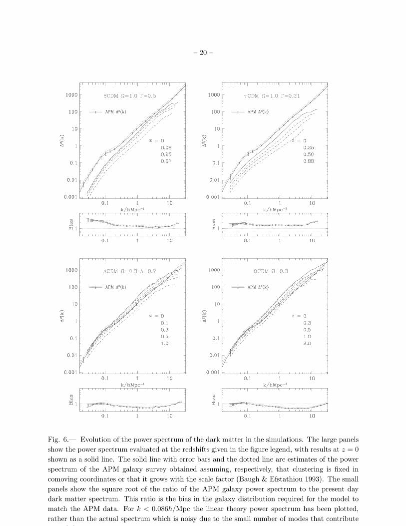
Fig. 6.— Evolution of the power spectrum of the dark matter in the simulations. The large panels

show the power spectrum evaluated at the redshifts given in the figure legend, with results at z = 0

shown as a solid line. The solid line with error bars and the dotted line are estimates of the power

spectrum of the APM galaxy survey obtained assuming, respectively, that clustering is fixed in

comoving coordinates or that it grows with the scale factor (Baugh & Efstathiou 1993). The small

panels show the square root of the ratio of the APM galaxy power spectrum to the present day

dark matter spectrum. This ratio is the bias in the galaxy distribution required for the model to

match the APM data. For k < 0.086h/Mpc the linear theory power spectrum has been plotted,

rather than the actual spectrum which is noisy due to the small number of modes that contribute

to each bin.

– 21 –

any scale with adequate sampling and avoid this problem except for m = 1.

The assumption that these sparsely sampled modes carry representative power is true by

construction in the initial conditions. The violation of this assumption as a result of nonlinear

evolution is very unlikely because it would require a detailed large-scale ordering to develop over

the simulation. This may, however, come about artificially; for example, the MAPS procedure of

Tormen and Bertschinger (1996, see also Cole 1997), which is designed to extend the dynamic

range of an N-body cosmological simulation, requires periodically replicating a simulation and

then modifying the large-scale modes so as to effectively add large-scale power not present in

the original simulation. In this case, the large-scale order arising by the replication introduces

significant fine scale structure in k-space (Cole 1997) and one should be wary when applying this

method.

Figure 6 shows the time evolution of the power spectrum for the same four simulations

(L = 239.5h−1Mpc) illustrated in Figure 5. As before, two graphs are shown for each model. The

larger one gives the time evolution of the power spectrum, plotted at four different epochs. The

z = 0 results may be compared with the 3D power spectrum of the APM galaxy survey (Baugh

& Efstathiou 1993). As for the correlation function, two versions of the APM power spectrum

are plotted, one assuming that the clustering pattern remains fixed in comoving coordinates

(solid curve with error bars) and the other assuming that it evolves in proportion to the scale

factor (dotted curve). For wavenumbers k < 0.086h/Mpc we have plotted the linear theory

power spectrum rather than the simulation results since the sparse sampling of the modes with

wavelength comparable to the simulation box size gives rise to spurious fluctuations. The linear

extrapolation can be seen to join smoothly onto the actual power spectrum on these scales. The

smaller panels show the square root of the ratio of the APM galaxy power spectrum to that of the

dark matter in the simulation at z = 0. As before, this is the scale-dependent bias required in the

galaxy distribution for a particular model to be a good match to the APM data.

Comparison of the APM data with the power spectrum of the dark matter in the different

cosmological models brings out essentially the same features as the corresponding comparison with

the correlation function. In the SCDM model, the dark matter power spectrum falls below that

of the galaxies at small wavenumbers, requiring a bias function that increases rapidly at small k.

The shape of the power spectrum in the low-Ω0 models is similar to that of the APM galaxies

only for k < 0.1h/Mpc; at larger k the dark matter distribution has more power than the galaxy

distribution, requiring a bias less than unity. Only the τCDM model has a dark matter power

spectrum whose shape matches that of the galaxy data over a wide range of scales. The required

bias in this case is approximately constant for 0.02 ∼< k/hMpc−1∼< 10.

– 22 –

7. Comparison with analytic predictions

We now compare the results of our simulations with a parameterised fitting formula which

Peacock & Dodds (1996) use to predict the power spectrum of the nonlinear mass density field

which develops through gravitational amplification of any given gaussian field of linear density

fluctuations. We consider both the power spectrum and the correlation function. We first

summarise the theory and then compare it with the simulation results discussed in Sections 5

and 6.

7.1. Method

Hamilton et al. (1991) suggested a formalism for computing the nonlinear growth of the

two-point correlation function. Peacock & Dodds (1994) adapted this method to the computation

of nonlinear power spectra, and extended it to cosmologies with Ω0 6= 1. Baugh & Gaztanaga

(1996) applied it to the power spectrum of the APM galaxy survey. The original formalism of

Hamilton et al. (1991) was independent of the shape of the power spectrum, but Jain, Mo & White

(1995) showed that this is not correct. Peacock & Dodds (1996) give an improved version of the

Peacock & Dodds (1994) method which takes this into account and allows the nonlinear spectrum

produced by evolution from any smoothly-varying linear spectrum to be calculated. Smith et al.

1997 have tested the new procedure with a large number of N-body simulations. The method may

be summarized as follows.

The nonlinear spectrum is a function of the linear spectrum at a smaller linear wavenumber:

∆2NL

(kNL) = fNL[∆2L(kL)], (8)

kL = [1 + ∆2NL

(kNL)]−1/3kNL. (9)

The following fitting formula for the nonlinear function, fNL was proposed by Peacock & Dodds

(1996):

fNL(x) = x

[

1 + Bβx + [Ax]αβ

1 + ([Ax]αg3(Ω0)/[V x1/2])β

]1/β

. (10)

In this expression, B describes a second-order deviation from linear growth; A and α parametrise

the power-law which dominates the function in the quasi-linear regime; V is the virialisation

parameter which gives the amplitude of the fNL(x) ∝ x3/2 asymptote (where the behaviour enters

the “stable clustering” limit); and β softens the transition between these regimes. For power

spectra of the form |δ2k| ∝ kn, the parameters and their dependence on n are:

A = 0.482 (1 + n/3)−0.947

B = 0.226 (1 + n/3)−1.778

α = 3.310 (1 + n/3)−0.244 (11)

– 23 –

β = 0.862 (1 + n/3)−0.287

V = 11.55 (1 + n/3)−0.423.

The growth factor, g(Ω), is proportional to the ratio of the linear growth factor to the expansion

factor. It takes the value unity for Ω = 1 and, for Ω0 < 1, it tends to unity as Ω → 1.

For linear spectra which are not a power-law, particularly for the CDM model, Peacock &

Dodds (1996) suggested that a tangent spectral index as a function of linear wavenumber should

be used:

neff(kL) ≡d ln P

d ln k(k = kL/2). (12)

The factor of 2 shift to smaller k is required because the tangent power-law at kL overestimates

the total degree of nonlinearity for curved spectra in which neff is a decreasing function of k and

underestimates it in the opposite case. Peacock & Dodds (1996) state that this prescription is able

to predict the nonlinear evolution of power-law and CDM spectra up to ∆2 ≃ 103 with an rms

precision of about 7%. Since the fitting formula is designed to reproduce the results for power-law

spectra, the main uncertainty in this method is whether or not the shifted tangent power-law is

the best means of deducing the effective n as a function of scale. This issue becomes especially

important when the effective index is more negative than −2 (because nonlinear effects diverge as

n → −3), and when the curvature of the spectrum is especially severe. This means that spectra

with low values of Ω0h or of σ8 present the greatest challenge for the analytic method.

The effect of cosmology enters into the fitting formula only through the growth factor, g(Ω),

which governs the amplitude of the virialised portion of the spectrum.

7.2. Fit to the simulations.

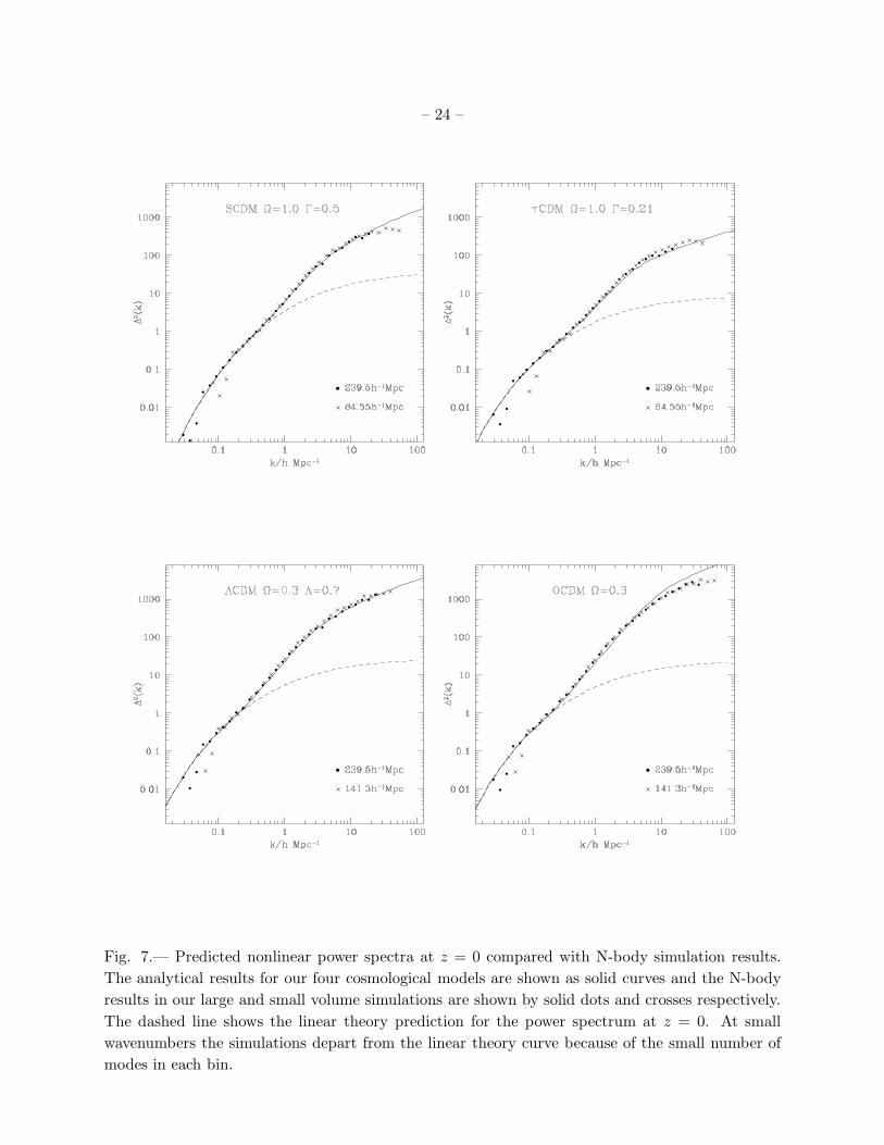
The nonlinear power spectrum predicted by eqn (11) for each of our four cosmological models

is plotted as a solid line in Figure 7. The solid circles and crosses show the results from our

large and small volume simulations respectively. Note the excellent agreement between them.

The dashed curve shows the linear theory prediction for the present day power spectrum2. The

points are plotted only on scales where the power exceeds the shot noise. The agreement between

the analytical and numerical results is generally good, particularly for SCDM and ΛCDM. For

all the models with Γ = 0.21, the predicted power spectrum slightly underestimates the detailed

power spectrum of the simulations around the region ∆2 ≃ 10. As discussed above, these cases

2The realisation of the power spectrum in our simulations can be seen to have a downward fluctuation in power

at 1 ≤ |kL/2π| < 2, where L is the simulation box size. A χ2 test for these 26 modes shows that a fluctuation lower

than this is expect in 7% of cases. While this fluctuation is not particularly unusual, it has little effect on the results

of interest (except for bulk flows; c.f. §3.1, §5 and §8) because our simulated volumes are sufficiently large.

– 24 –

Fig. 7.— Predicted nonlinear power spectra at z = 0 compared with N-body simulation results.

The analytical results for our four cosmological models are shown as solid curves and the N-body

results in our large and small volume simulations are shown by solid dots and crosses respectively.

The dashed line shows the linear theory prediction for the power spectrum at z = 0. At small

wavenumbers the simulations depart from the linear theory curve because of the small number of

modes in each bin.

– 25 –

Fig. 8.— Predicted mass correlation functions at z = 0 compared with N-body simulation results.

The analytical results for our four cosmological models are shown as solid curves and the N-body

results in our large and small volume simulations are shown by solid dots and crosses respectively.

The dashed line shows the linear theory prediction for ξ(r) at z = 0. At large pair separations

the integral constraint in the smaller simulations depresses ξ(r) slightly, whereas at small pair

separations, ξ(r) is slightly higher in the smaller volumes because they have better mass resolution.

– 26 –

are expected to be especially challenging, because they have a more negative neff at the nonlinear

scale. The slight mismatch illustrates the difficulty in defining precisely the effective power-law

index for these rather flat spectra, and a more accurate formula could be produced for this

particular case, if required. Note that in the quasilinear portion the power spectra follow very

closely the general shape predicted by eqns (8)-(12); in particular, there is essentially no difference

between the OCDM and ΛCDM results, as expected.

The power spectra of the different cosmological models are expected to part company at

higher fequencies, where the spectrum enters the “stable clustering” regime, and indeed they do.

However, although the predictions match the ΛCDM results almost precisely at ∆2 ≃ 1000, they

lie above the OCDM results at high k: ∆2(k = 30) ≃ 4500, compared to the simulation value of

2500. At one level, this is not so surprising, since the smaller simulations that Peacock & Dodds

(1996) used to derive the parameters of the fitting formula were not able to resolve scales beyond

∆2 ≃ 1000. However, the amplitude of the stable clustering asymptote is very much as expected

in the Ω = 1 and ΛCDM cases, and the argument for how this amplitude should scale with Ω0 is

straightforward: at high redshift, clustering in all models evolves as in an Ω = 1 universe, and so

evolution to the present is determined by the balance between the linear growth rate and the (Ω0

independent) rate of growth of stable clustering. The failure of this scaling for the OCDM case is

therefore something of a puzzle. It is conceivable that the numerical result could be inaccurate,

since it depends on resolving small groups of particles with overdensities of several thousand, and

these collapse very early on. However, we have verified that changing the starting redshift from 59

to 119 does not alter the results of the simulations significantly.

Figure 8 shows the two-point correlation function derived using eqn (7) and the predicted

nonlinear power spectrum, eqns (8)-(12). As before, the N-body results are plotted as filled

circles and crosses for the large and small volume simulations respectively. Note that in general,

the agreement between each pair of simulations is very good and the very small discrepancies

that there are can be understood simply. At large pair separations ξ(r) is slightly depressed in

the smaller simulations because these separations are becoming an appreciable fraction of the

box length and the integral constraint requires ξ(r) to average to zero over the volume of the

simulation. At small pair separations, ξ(r) is slightly higher in the smaller volumes because of

their higher mass resolution. Once again, there is good agreement in general between the anlytical

predictions and the N-body results, particularly for the ΛCDM and SCDM models. For τCDM,

the model underpredicts the correlation function on scales below 700h−1kpc whilst for OCDM,

the model correlation function is somewhat steeper than in the simulations. These differences

occur on scales significantly larger than those affected by resolution effects, and are fully consistent

with the analogous deviations seen in the power spectrum.

– 27 –

8. The Velocity Fields and distributions.

In this section we compute bulk flows, velocity dispersions, and pairwise velocities of the

dark matter particles in our simulations. Potentially, measurements of galaxy peculiar velocities

can provide powerful tests of the models. In practice, there are a number of complications which

weaken these tests. Foremost amongst them is the uncertain relation between the velocity fields

of dark matter and galaxies, particularly on small scales where various dynamical biases may

operate (Carlberg, Couchman & Thomas 1990, Frenk et al. 1996). It is relatively straightforward

to calculate, with high precision, the velocity fields of the dark matter in a given cosmology,

using simulations like ours or, in the appropriate regime, using linear theory. To relate these to

observations on small scales requires an understanding of possible dynamical biases and, in the

case of pair-weighted statistics, of sampling uncertainties and systematic effects arising from the

discrete nature of the galaxy population. Only on sufficiently large scales do we expect galaxy

bulk flows which are, in principle, measurable to be simply related to the dark matter bulk flows.

Observational determinations of galaxy velocities have their own complications. For example,

determining bulk flows over representative volumes requires measuring peculiar velocities, and thus

determining distances with an accuracy of a few percent, for large samples of galaxies. Defining

such samples in a homogeneous way and keeping systematic effects in the distance measurements

within tolerable levels is a complex and still uncertain process (e.g. Willick et al. 1997). Other

measures of the galaxy velocity field such as the pairwise relative velocities of close pairs are also

affected by systematic and sampling effects even though they do not require measuring distances

(e.g. Marzke et al. 1995; Mo, Jing & Borner 1996.)

In view of the various uncertainties just mentioned, we focus here on high precision estimates

of various measures of the dark matter velocity field. Our main purpose is to contrast the velocity

fields predicted in the four cosmological models considered in this paper, in the expectation that

these and related calculations may eventually be applied to a reliable interpretation of real galaxy

velocity fields. We do, however, carry out a limited comparison of dark matter velocity fields with

existing data on large-scale galaxy bulk flows and pairwise velocity dispersions. In subsection 8.1

we compute distributions of the mean and rms dark matter velocity on various scales and in

subsection 8.2 we consider pairwise velocities also over a range of scales.

8.1. Bulk flows and dispersions.

We compute bulk flows and velocity dispersions of dark matter particles in the simulations by

placing a large number of spheres of varying radii around random locations in the computational

volume. We define the bulk velocity of a sphere as:

V =1

N

∑

i=1,N

vi (13)

– 28 –

0 20 40 60 800

100

200

300

400

500

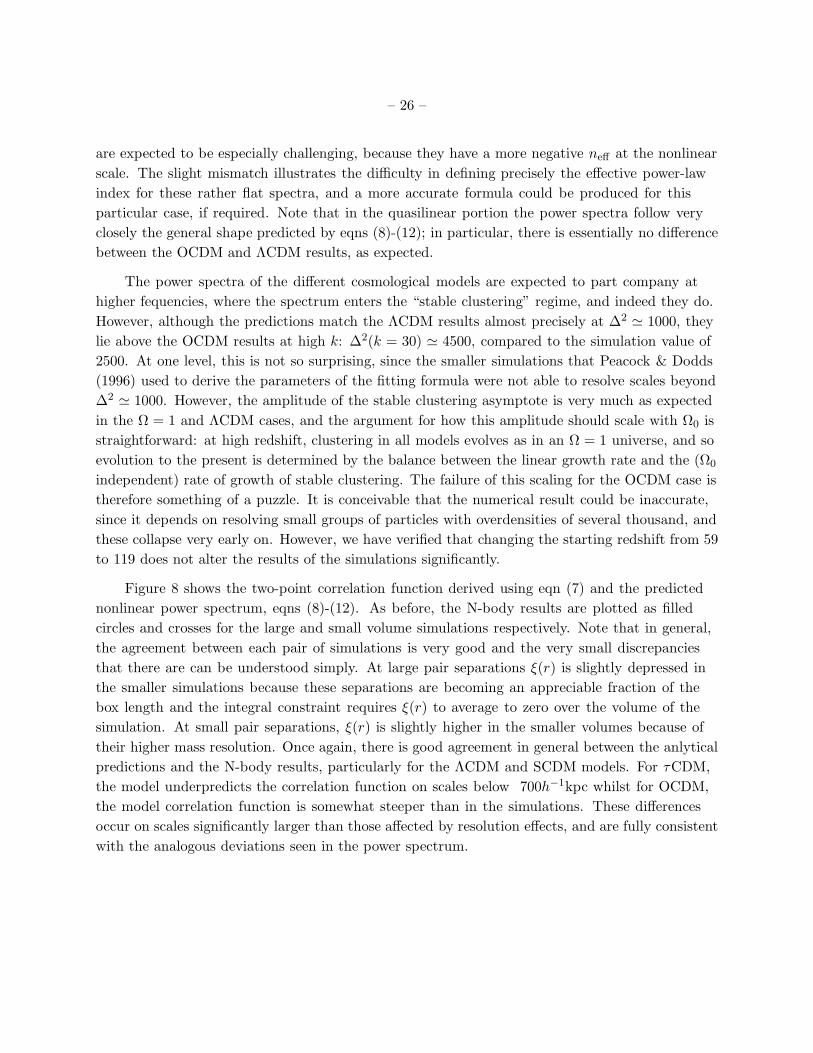
Fig. 9.— Comparison of the bulk flow measured in the τCDM model (solid circles) with linear

theory. The long-dashed curve is the linear theory result in the limit of an infinite box size. The

dotted line with error bars shows the ensemble rms average for a 239.5h−1Mpc periodic box. The

error bars give the rms spread between different realisations. The solid line is the result from

linear theory for the realisation used in our τCDM simulation. Linear theory works to excellent

approximation when all the finite box effects are taken into account.

– 29 –

where vi is the peculiar velocity of the ith particle out of N in a given sphere and all particles

have equal weight. The dispersion σv is defined as:

σ2v =

1

N − 1

∑

i=1,N

(vi − V)2 (14)

In linear theory, the bulk velocity of the dark matter can be accurately calculated according

to:

< V 2 >= Ω1.20

∫ ∞

0k−2W 2(Rk)∆2(k)

dk

k(15)

where W (Rk) is a window function, which we take to be a top hat of radius R in real space.

The approximate factor Ω1.20 works well for all the cosmological models we are considering here

(Peebles 1980.)

The integral in eqn (15) ranges over all spatial scales and so applies to a simulation only in the

limit of an infinite volume. In order to compare the simulations with linear theory it is necessary

to take account of effects due to the finite computational box and of the fact that we have only

one realisation. Finite box effects are much more significant for velocities than for the correlation

function (eqn 6), since the relative importance of longer waves is enhanced in eqn (15) by a factor

k−2. To compare linear theory with a specific simulation, the integral in expression (15) must be

replaced by a summation over the modes of the periodic box, using the appropriate power in each

mode as set up in the initial conditions.

The dashed curve in Fig 9 shows the linear theory prediction for bulk flows at z = 0, in

spheres of radius Rsphere, for a model with the power spectrum and normalisation of our τCDM

simulation, in the limit of infinite volume. The predicted velocities fall off smoothly from about

500 kms−1 at 10h−1Mpc to about 200 kms−1 at 100h−1Mpc. The dotted curve shows the linear

theory ensemble average value of < V 2 >1/2 over realizations of the τCDM power spectrum in

volumes the size of our simulation. The difference between this and the dashed curve indicates

just how important finite box effects are in computing bulk flows. The error bars on the dotted

curve show the rms dispersion amongst different realizations. For small spheres, the variation

about the mean is approximately Gaussian and the error bars may be regarded as 1-σ deviations

from the mean. The results from our actual simulation at z = 0 are plotted as solid circles in

the figure and the linear theory prediction for evolution from the specific initial conditions of this

simulation is shown as the solid curve. The particular realisation that we have simulated turned

out to produce slightly, but not anomalously, low velocities. On scales above 20h−1Mpc the linear

theory prediction agrees very well with the simulation; at R = 10h−1Mpc, it overestimates the

actual velocities by 5%.

While linear theory suffices to calculate bulk flows on scales larger that about 10h−1Mpc, the

velocity dispersion of particles in spheres is dominated by contributions from nonlinear scales and

must be obtained from the simulations. Finite box effects are not important in this case because

the contributions from wavelengths larger than the simulation box are small.

– 30 –

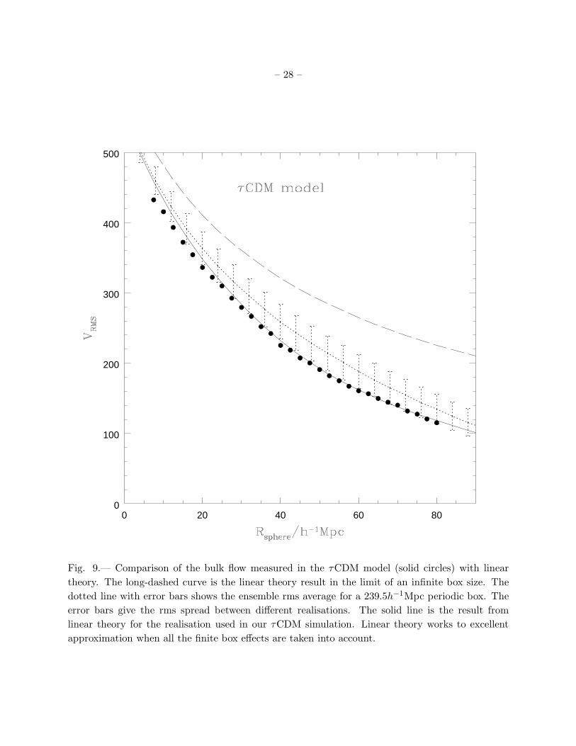
The bulk flows, < V 2 >1/2, calculated from linear theory and the velocity dispersions in

spheres, σv, calculated from our L = 239.5h−1Mpc simulations are plotted as solid lines in Fig 10

for our four cosmological models. The dotted curves around the < V 2 >1/2 curve correspond to

90% confidence limits on the bulk velocity for a randomly placed sphere, calculated by integrating

over the appropriate Raleigh distribution. The dotted curves around the σv curve indicate the rms

scatter of the σv distribution.

With the exception of SCDM the predicted bulk flows in all our models are remarkably

similar. The reason for this can be traced back to our choice of normalisation which ensures that

all models produce approximately the same number of rich galaxy clusters. This choice effectively

cancels out the dependence of the bulk flow velocity on Ω0 as may be seen directly from linear

theory. From eqn (15), < V 2 >1/2∝ σ8Ω0.60 , for a fixed shape of the power spectrum. On the other

hand, our adopted fluctuation normalisation requires approximately that σ8 ∝ Ω−0.50 (cf. eqns 1

and 2). Since the power spectra of the ΛCDM, τCDM, and OCDM models all have the same

shape parameter, Γ = 0.21, the bulk flows in these models are very similar. The lower bulk flow

velocities predicted in the SCDM model reflect the relatively smaller amount of large scale power

in this model implied by its value of Γ = 0.5. The mean bulk velocity in SCDM is approximately

2/3 of the value in the other models.

The peculiar velocity dispersion of dark matter particles in random spheres is also remarkably

similar in all our models, including SCDM. In this case, significant contributions to σv come from

a wide range of scales, including nonlinear objects as well as regions which are still in the linear

regime. On small scales, σv rises with increasing sphere radius and reaches a plateau at radii of

a few tens of megaparsecs. The limit as the radius tends to infinity is just the single particle rms

peculiar velocity. For our large simulation boxes, this is 614 kms−1, 635 kms−1, 648 kms−1 and

630 kms−1 for the SCDM, τCDM, ΛCDM and OCDM models respectively. The slightly lower

value for SCDM again reflects the smaller large-scale power in this model compared to the others.

This deficit on large scales, however, is compensated by an excess contribution from smaller scales.

We have plotted in Figure 10 estimates of galaxy bulk flow velocities in the local universe

taken from the analyses by Mould et al. (1993), Courteau et al. (1993), Dekel et al. (1997), and

Lauer & Postman (1994). These estimates are based on different datasets and assumptions and,

apart from the Lauer & Postman measurement, they are broadly consistent with one another,

although the Mould et al. measurement is somewhat high. The data from the first three surveys

are broadly consistent with the predictions of all our models except SCDM which produces

velocities about factor of 2 lower than the data on large scales. None of the models is consistent

with the measurement of Lauer & Postman who inferred a bulk flow of 764 ± 160 kms−1 (as

reanalysed by Colless 1995) on a scale of ∼ 80h−1Mpc from a sample of brightest cluster galaxies.

The results in the figure show that bulk flows are insensitive to the value of Ω0 when one focusses

attention on models that agree with the observed cluster abundance. If anything, observed bulk

flows constrain the shape of the power spectrum on large-scales or, in the case of the Lauer &

Postman result, they conflict with the entire class of models we are considering.

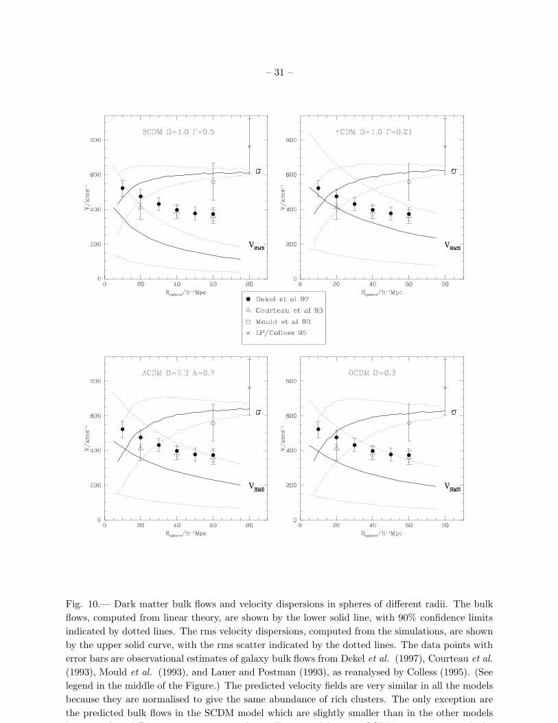
– 31 –

Fig. 10.— Dark matter bulk flows and velocity dispersions in spheres of different radii. The bulk

flows, computed from linear theory, are shown by the lower solid line, with 90% confidence limits

indicated by dotted lines. The rms velocity dispersions, computed from the simulations, are shown

by the upper solid curve, with the rms scatter indicated by the dotted lines. The data points with

error bars are observational estimates of galaxy bulk flows from Dekel et al. (1997), Courteau et al.

(1993), Mould et al. (1993), and Lauer and Postman (1993), as reanalysed by Colless (1995). (See

legend in the middle of the Figure.) The predicted velocity fields are very similar in all the models

because they are normalised to give the same abundance of rich clusters. The only exception are

the predicted bulk flows in the SCDM model which are slightly smaller than in the other models

because of its different power spectrum shape. Every model except SCDM is consistent with the

– 32 –

8.2. Pairwise velocities

We now consider the lower order moments of the pairwise velocity distribution of dark matter

particles in our four cosmological models. Specifically, we consider the following quantities: v21,

the mean radial peculiar velocity of approach between particle pairs; v2‖ , the dispersion in the

radial velocities of pairs; and v2⊥, the dispersion in the mean transverse relative velocities of

pairs. Following standard practice, v2‖ is not centered; to center one just needs to subtract v21 in

quadrature. These quantities are not directly observable, but we also compute the dispersion, σ2los,

the line-of-sight velocity dispersion (this time centered), defined as:

σ2los(r) =

∫

ξ(R) σ2proj(R) dl

∫

ξ(R) dl(16)

where r is the projected separation, R =√

r2 + l2, and the the integral is taken along the

line-of-sight between ±25h−1Mpc. The quantity σ2proj is the line-of-sight centred pairwise

dispersion which is given by:

σ2proj =

r2v2⊥/2 + l2(v2

‖ − v221)

r2 + l2(17)

This quantity is somewhat closer to measurements accesible in galaxy redshift surveys; it is a

much weaker function of apparent separation than v2‖ and v2

⊥.

Figure 11 shows v21, v‖, v⊥ and σlos as a function of pair separation in our models. Also

drawn on each panel is the Hubble line, given by vHubb = −Hr, where H is Hubble’s constant and

r is pair separation in physical units. Pairs at fixed physical separation lie on this line. In the

stable clustering regime (Peebles 1980), v21 must follow vHubb. The distance at which the mass

correlation function equals unity, the correlation length, is marked by an arrow.

The mean pairwise radial velocities, v21, vanish at the smallest separations resolved in our

simulations. In the low-Ω0 models, where the growth of structure is freezing out at low redshift,

v21 follows the Hubble line up to scales ∼ 300h−1kpc. This indicates that structures on these

scales have almost completely relaxed and the clustering is stable. In the Ω = 1 models there is

still a net radial inflow on these scales although the inflow timescale is longer than the Hubble

time and very much longer than the local dynamical time of pairs at these separations (where

ξ(r) = 80 − 200); the latter is, in turn, much shorter than the Hubble time. The pairwise radial

velocity in these models reaches a peak inside the correlation length (marked by the arrow),

around 2− 3h−1Mpc. This indicates the typical scale of virialising structures at z = 0 in the Ω = 1

models. At larger radial separations v21 intersects the Hubble line and, at very large separations,

it decays to zero, in accordance with the principle of large-scale isotropy and homogeneity.

For the same reasons, one expects the ratio v2⊥/v2

‖ to tend to√

2 = 1.414 at large separations.

The measured ratios at a separation of 80h−1Mpc are 1.38, 1.34, 1.36 and 1.37 for SCDM, τCDM,

ΛCDM, and OCDM. At scales of a few h−1Mpc, where radial infall is at its most important,

the ratio in the SCDM model is about 1.23 (after centering). At smaller scales still, the relative

– 33 –

Fig. 11.— Pairwise velocity statistics. In each panel, the dotted curve is the mean inward radial

velocity v21; the short dashed line is the dispersion in the pairwise radial peculiar velocities v‖;

the long dashed line is the dispersion in the relative pairwise tangential peculiar velocities, v⊥;

the solid line is the line-of-sight dispersion, σlos; and the dot-dashed line is the Hubble line given

by vHubb = −Hr, where H is Hubble’s constant r is physical separation. The dispersion v‖ is

uncentered; to center, subtract v21 in quadrature. The data points are taken from Jing, Mo and

Borner (1997) and show the pairwise velocity dispersion, σ12 estimated for the Las Campanas

redshift survey. These points should be compared to the line-of-sight dispersions for the models.

See main text for discussion of the error bars used on these points.

– 34 –

motions inside virialised structures again become closer to isotropy, in agreement with results

from high resolution simulation of dark halos (Tormen 1996, Thomas et al. 1997). On very small

scales, two-body effects contribute to the isotropization of the orbits.

As was the case with the mean bulk flows and velocity dispersions in random spheres discussed

in subsection 8.1, the moments of the pairwise velocity distribution are very similar in the different

cosmologies. As before, this similarity is a direct consequence of our adopted normalisation. The

largest differences occur between the OCDM and τCDM models on small scales - a difference

of about 200 kms−1 in σlos. Qualitatively, the trends seen in Fig 11 agree with the analytical

calculation of Mo et al. (1996) who find that pairwise velocities in open models are slightly larger

than in Λ models and these, in turn, are larger than in Ω = 1 models.

It is difficult to compare the predicted dark matter pairwise velocities with galaxy

measurements for a variety of reasons. Firstly, the velocity dispersion of the dark matter

distribution in the simulations includes a contribution from the internal dispersion of virialized

halos. Secondly, there is some evidence that the velocity dispersion of dark halos in simulations

may be biased low relative to the dark matter velocity dispersion even after allowing for

contamination from virialized halos (Carlberg & Couchman 1989), an effect which Carlberg,

Couchman & Thomas (1990) argue is due to dynamical friction (see also Zurek et al. 1994). (The

velocities of the dark matter halos in our simulations will be analysed in a future paper by Frenk

et al. 1997.) Finally, biases in the spatial distribution of galaxies may introduce further biases

in the pairwise velocity statistics of the galaxies relative to the dark matter (Fisher et al. 1994,

Weinberg 1995, Evrard, Summers & Davis 1994.)

Observationally, the velocity dispersion of galaxy pairs is determined by fitting a model under

certain assumptions regarding the two-point correlation function and the spatial dependence of

the infall velocity and dispersion (Davis & Peebles 1983.) These assumptions do not necessarily

match the simulation data. More importantly, as Marzke et al. (1995) and Mo et al. (1996) have

argued, pairwise velocity statistics are not robust when determined from relatively small redshift

surveys since these statistics contain significant contributions from galaxy pairs in rare, massive

clusters. This is not a problem in our simulations which sample a volume of 13.8× 106(h−1Mpc)3,

but it is a problem in the present generation of redshift surveys with the possible exception of

the Las Campanas Redshift Survey (Shectman et al. 1996, hereafter LCRS.) Estimates of the

pairwise velocity dispersion in the LCRS, obtained by Jing et al. (1997), are shown as data points

in Figure 11. The LCRS contains quite a number of rich clusters and appears to give consistent

estimates when split into Northern and Southern subsamples. The error bars plotted in the figure

are the sum in quadrature of the errors obtained directly from the data by Jing et al. (1997) plus

the 1σ uncertainties found from applying the same estimator to mock catalogues constructed

from N-body simulations by these authors. The LCRS velocities are substantially larger than

most previous determinations. The dispersion remains approximately constant over the range

0.15 − 10h−1Mpc, reaching an amplitude of 570 ± 80 kms−1 at 1h−1Mpc.

– 35 –

The LCRS data may be compared with the line-of-sight dispersions plotted for each of our

simulations in Figure 11. At pair separations ∼> 2h−1Mpc, all our models are consistent with the

data, although the low-Ω models lie somewhat low. At smaller separations, all model curves rise

above the data. This difference in behavior may be due, in part, to the different methods for

estimating the dispersion in the simulations and the data, but it very likely reflects also the biases

present in the simulations mentioned earlier. Interestingly, the Ω = 1 models are closer to the

data on small scales than the low-Ω models, implying that substantially stronger velocity biases

are required in low-Ω models to bring them into agreement with the data.

9. Discussion and conclusions

We have used a suite of high resolution N-body simulations to investigate the clustering

evolution of dark matter in four different cold dark matter cosmologies. Our simulations followed

approximately 17 million particles. Most of our analysis is based on simulations of very large

cosmological volumes (239.5h−1Mpc)3, but we also analysed simulations of somewhat smaller

volumes and correspondingly higher mass resolution. The large volumes and particle numbers,

together with a relatively small gravitational softening (∼ 30h−1kpc), allow us to calculate the

clustering and kinematical properties of the dark matter with unprecedented accuracy. For

example, we are able to determine the mass autocorrelation function over nearly 3 decades in pair

separation with better accuracy than in previous simulations and also with higher precision than

is attainable with existing or planned surveys of galaxies. Our model mass correlation functions

are well fit by an analytic model of the type proposed by Hamilton et al. (1991) but with the

form and parameters proposed by Peacock & Dodds (1996). This model may therefore be used to

extend some of the results of our analysis to cosmologies with different parameter values to those

assumed in our simulations.

Two of the four variants of the CDM cosmology that we have investigated are motivated

by various lines of astronomical evidence which suggest a low cosmological density parameter,

Ω0 ≃ 0.3, and a spectral shape parameter, Γ = 0.21; we study both a flat model with a non-zero

cosmological constant (ΛCDM) and an open model (OCDM). The remaining two models both

have Ω = 1, but one has the standard power spectrum (SCDM) and the other has Γ = 0.21

(τCDM). In all cases, we have chosen to normalise the primordial fluctuation spectrum so that the

present abundance of rich clusters is approximately reproduced in all the models. We regard this

choice as preferable to the often used alternative of normalising to the amplitude of the COBE

microwave background anisotropies. With standard assumptions (a Harrison-Zeldovich primordial

spectrum and no contribution to the anisotropy from tensor modes), the cluster normalisation is

close to the COBE normalisation for the ΛCDM and τCDM models, but it is significantly higher

for the OCDM and significantly lower for the SCDM model. With our choice of normalisation, the

overall appearance of all models is determined primarily by their σ8 values with the result that the

two high density models look very similar while the two low density models show more structure

– 36 –

but resemble each other closely.

Our main results concern the detailed properties of the spatial distribution and velocity fields

of the dark matter at z = 0. We now discuss our results and display them concisely in Table 2. In

all the models the shape of the two-point correlation function, ξ(r), and power spectrum, ∆2(k),

of the dark matter differ significantly from those of the observed galaxy distribution. In particular,

they fail to reproduce the accurate power-law which the APM survey (and others before that; c.f.

Groth & Peebles 1977) exhibits over nearly four orders of magnitude in amplitude. At small, but

still well-resolved pair separations, all our model correlation functions become shallower, while at

intermediate separations they all have an inflection point. Uniquely amongst the models we have

explored, τCDM has a mean correlation slope which is approximately correct over the bulk of

the observable range, but even in this case there are substantial discrepancies on scales smaller

than ∼ 0.2h−1Mpc. Thus, for any of these models to provide an acceptable representation of

reality, the distribution of galaxies would need to be biased relative to the mass in a non-trivial,

scale-dependent, fashion. Whatever the processes involved in biasing the galaxy distribution may

be, they must conspire to iron out the features in the dark matter correlation function.

We define a “bias function” as the square root of the the ratio of the galaxy to the mass

autocorrelation functions. Our simulations, together with the galaxy autocorrelation function

measured from the APM survey by Baugh (1996), give the bias as a function of scale accurately

for the four models we have investigated. We find that our two Ω = 1 models require a bias

greater than unity everywhere. In the SCDM case, the bias grows from ∼ 1 at ∼ 1h−1Mpc to

∼ 1.5 at ∼ 8h−1Mpc and rises sharply beyond that. In the τCDM model the bias is approximately

constant, at b ≃ 1.5, between ∼ 0.2h−1Mpc and ∼ 20h−1Mpc.

By design, our low-Ω0 models have a power spectrum that approximates that of the APM

galaxy survey on large scales. However, even in this case, the match is not perfect and some

amount of bias may still be required at separations > 10h−1Mpc. Furthermore, these models have

the undesirable feature that the mass correlation function rises above the APM galaxy correlation

function at pair separations smaller than ∼ 5h−1Mpc. On these scales, an “antibias” is required

for these models to match the observed galaxy clustering. Galaxy mergers in high density regions

may plausibly suppress small-scale correlations, but it remains to be seen whether an antibias of

the required magnitude is achievable in practice. Antibiasing may be difficult to reconcile with

observed cluster mass-to-light ratios. In standard virial analyses of clusters, a value of Ω0 is

derived from the measured mass-to-light ratio by assuming that the galaxies cluster just like the

mass. With this assumption Carlberg et al. (1997), for example, inferred Ω0 = 0.19±0.06 from the

CNOC sample of intermediate redshift clusters. If galaxies were actually antibiased, this estimate

of Ω0 would need to be corrected downwards. However, models with lower values of Ω0 require

higher values of σ8, and even stronger antibias, in order to reproduce the observed abundance of

clusters.

Our simulations allow us to calculate accurately the velocity fields of the dark matter over a

– 37 –

wide range of scales. These are very similar in all our models, whether they be characterised as

bulk flows, single-particle or pairwise velocity dispersions. This similarity in the velocity fields is

a direct consequence of our adopted normalisation and runs contrary to the common belief that

the amplitude of the observed galaxy velocity fields can be used to constrain the value of Ω0. A

residual dependence of the velocity field on the shape of the power spectrum causes the velocities

in the SCDM model to be somewhat lower than in the other models, but amongst the latter

there is no discernible difference. For example, the 1D velocity dispersion of the dark matter is

approximately 600 kms−1 in all the models, and the line-of-sight pairwise velocity dispersions fall

in the range 700 − 900 kms−1. The first of these numbers is reminiscent of the peculiar velocity

of the Local Group, while the second is consistent with, although on the high side of, a recent

determination from the Las Campanas redshift survey at a pair separation of ∼ 1h−1Mpc (Jing

et al. 1997). On smaller scales, our simulations, particularly our low-Ω0 models, predict higher

pairwise velocity dispersions than inferred from this survey, indicating that a substantial velocity

bias is required to bring the models into agreement with the data. Bulk flows on large-scales are

most accurately calculated using linear theory. Our models all predict somewhat smaller values

than those estimated from recent surveys of the local universe (Mould et al. 1993; Courteau et al.

1993; Dekel et al. 1997) but, with the exception of SCDM, they are consistent with these data.

None of the models reproduces the large bulk flows inferred by Lauer & Postman (1994).

High resolution simulations like those presented here allow very accurate measurements of the

clustering distribution of dark matter. Further progress in this subject will rely on the ability to

address the outstanding issue that limits the comparison of these models with observations: the

connection between the distribution of mass and the distribution of galaxies. This will require a

realistic treatment of the evolution of the baryonic component of the Universe.

We are grateful to Carlton Baugh for useful discussions and for providing us with the APM

galaxy survey data used in Figures 5 and 6. We thank David Weinberg for suggesting several

significant improvements to the manuscript and Avishai Dekel for communicating to us, in advance

of publication, results of his bulk analysis shown in Figure 10. CSF acknowldeges a PPARC Senior

Fellowship. This work was supported in part by grants from PPARC, EPSRC and the EC TMR

network for “Galaxy formation and evolution.” The simulations reported here were carried on the

Cray-T3Ds at the Edinburgh Parallel Computing Centre and the Rechenzentrum, Garching. We

thank the Editor for suggesting the inclusion of Table 2.

– 38 –

A. Appendix: Derivation of equation (5)

The two-point correlation function is related to the power spectrum by:

ξ(r) =

∫

P (k) exp[ik · r]d3k, (A1)

where bold font implies that the quantity is a 3-dimensional vector.

In deriving a correction to the linear correlation function for a periodic box we must make an

assumption for how the power selected for each discrete mode of the periodic box is related to the

power density of the same mode in the continuous power spectrum. As discussed in Section 3.1,

we draw the power for each mode from an exponential distribution with the mean power set by

the power density of the mode in the continuous power spectrum. Thus, the ensemble-average

linear correlation function of the periodic boxes, ξs(r), is given by:

ξs(r) = (2π

L)3

∞∑

b=(0,0,0)

P (2πb

L) exp[2πib · r/L], (A2)

where L is the simulation boxsize and the sum over b is a sum over all integer triples. The

correction we derive is a systematic correction that applies to an ensemble of simulations.

We make use of the Poisson summation formula which, for a function φ(x), states that:

∞∑

b=(0,0,0)

φ(2πb) =1

(2π)3

∞∑

n=(0,0,0)

∫

φ(t) exp[in · t]d3t, (A3)

subject to certain conditions on the function φ(x) which hold for the case of interest here (see

Courant and Hilbert 1953, p.76).

Substituting the r.h.s. of equation (A2) into the Poisson summation formula we obtain:

ξs(r) =∞∑

n=(0,0,0)

∫

P (k) exp[ik·(r − Ln)]d3k. (A4)

From equation (A1) we can rewrite this as:

ξs(r) = ξ(r) +∞∑

n6=(0,0,0)

ξ(r − Ln) (A5)

Applying this to the evolved linear power spectrum, which is isotropic, we arrive at the correction

term, eqn (5), to the correlation function for the periodic box:

ξ(r) =∞∑

n6=(0,0,0)

−ξlin(|r + Ln|) (A6)

– 39 –

REFERENCES

Babul, A. & White, S. D. M. 1991, MNRAS, 251, 31

Bardeen, J. M., Bond, J. R., Kaiser, N. & Szalay, A. S. 1986, ApJ, 304, 15

Baugh, C. M. 1996, MNRAS, 280, 267

Baugh, C. M. & Efstathiou, G. 1993 MNRAS, 265,145

Baugh, C. M. & Gaztanaga, E. 1996 MNRAS, 280, 37

Bernardeau, F. 1994, ApJ, 433, 1

Bond, J. R. & Efstathiou, G. 1984, ApJ, 285, L45

Bond, J. R. & Efstathiou, G. 1991, Phys. Lett. B., 265,245

Bouchet, F. R., Colombi, S., Hivon, E. & Juszkiewicz, R. 1995,A&A, 296, 575

Bower, R. G., Coles, P., Frenk, C. S. & White, S. D. M. 1993, MNRAS, 405, 403

Carlberg, R. G. & Couchman, H. M. P. 1989, ApJ, 340, 47

Carlberg, R. G., Couchman, H. M. P & Thomas, P. A. 1990 ApJ, 352, L29

Carlberg, R. G., Yee, H. K. C. & Ellingson, E. 1997, ApJ, 478, 462

Cen, R. & Ostriker, J. P. 1992, ApJ, 399, 113

Centrella, J. & Melott, A. L. 1983, Nature, 305, 196

Cole, S., Weinberg, D. H., Frenk, C. S. & Ratra, B. 1997, MNRAS, 289, 37

Cole, S. 1997,MNRAS, 286, 38

Coles, P. 1993, MNRAS, 262, 1065

Colless, M. 1995, AJ, 109, 1937

Couchman, H. M. P., Thomas, P. A. & Pearce F. R. 1995, ApJ, 452, 797

Couchman, H. M. P., Pearce, F. R., Thomas, P. A. 1996, astro-ph/9603116

Courteau, S., Faber, S. M., Dressler, A. & Willick, J. A. 1993, ApJ, 412, L51

Courant, R. & Hilbert, D., 1953, Methods of Mathematical Physics.

Cray Research Inc, Cray MPP Fortran Reference Manual, SR-2504 6.1

Croft, R. A. C. & Efstathiou, G. 1994, MNRAS, 267, 390

– 40 –

Davis, M. & Peebles, P. J. E. 1983, ApJ, 267, 465

Davis, M., Efstathiou, G., Frenk, C. S. & White, S. D. M. 1985, ApJ, 292, 371

Dekel, A. & Rees, M. 1987, Nature, 326, 455

Dekel, A. et al. 1997, in preparation

Edge, A. C., Stewart, G. C., Fabian, A. C. & Arnaud, K. A. 1990, MNRAS, 245, 559

Efstathiou, G. & Eastwood J. W. 1981, MNRAS, 194, 503

Efstathiou, G., Davis, M., Frenk, C.S. & White, S. D. M. 1985, ApJS, 57, 241

Efstathiou, G, Kaiser, N., Saunders, W., Lawrence, A., Rowan-Robinson, M., Ellis, R. S. & Frenk,

C. S. 1990, MNRAS, 247, 10

Eke, V. R., Cole, S. & Frenk, C. S. 1996, MNRAS, 282, 263

Evrard, A. E., Summers, F. J. & Davis, M. 1994, ApJ, 422, 11

Evrard, A. E. 1997, astro-ph/9701148

Fisher, K. B., Davis, M. Strauss, M. A., Yahil, A. & Huchra, J. P. 1994, MNRAS, 267, 927

Frenk, C. S., White, S. D. M. & Davis, M. 1983, ApJ, 271, 471

Frenk, C.S., White, S.D.M., Efstathiou, G. & Davis, M. 1985, Nature, 317, 595

Frenk, C.S., White, S.D.M., Efstathiou, G. & Davis, M. 1988, ApJ, 327, 507

Frenk, C.S., White, S.D.M., Efstathiou, G. & Davis, M. 1990, ApJ, 351, 10

Frenk, C. S. 1991, Models of Large Scale Structure PhsS, 36, 70

Frenk, C. S., Evrard, A. E., White, S. D. M. & Summers, F. J. 1996, ApJ, 472, 460

Frenk, C. S. et al. 1997, in preparation

Fry, J., & Melott, A. 1995, ApJ, 292, 395

Garcia-Bellido, J. & Linde, A. 1997, CERN preprint CERN-TH/97-08

Gelb, J. M. & Bertschinger, E. 1994, ApJ, 436, 467

Gelb, J. M. & Bertschinger, E. 1994, ApJ, 436, 491

Giovanelli, R. 1997, in M. Liveo, M. Donohue & N. Panagia, eds The Extragalactic Distance Scale.

Cambridge University Press, New York, in press

– 41 –

Gorski, K. M., Ratra, B., Sugiyama N. & Banday, A. J. 1995, ApJ, 444, L65

Gott, J. R., Turner, E. L. & Aarseth, S. J. 1979, ApJ, 234, 13

Groth, E. J. & Peebles, P. J. E. 1977, ApJ218, 592

Gunn, J. & Weinberg, D. 1995, in Wide Field Spectroscopy and the Distant Universe, eds S. J.

Maddox & A. Aragon-Salamanca, World Scientific, p3

Guth, A. & Pi, S.-Y. 1981, Phys. Rev. Lett. 49, 1110.

Henry, J. P. & Arnaud, K. A. 1991, ApJ, 372, 410

Hamilton, A. J. S., Kumar P., Lu E. & Matthews A. 1991, ApJ, 374, L1

Henry, J. P. 1997, preprint

Jain, B., Mo, H. J. & White, S. D. M. 1995, MNRAS, 276, L25

Jain B., Mo H. J., White S. D. M. 1995, MNRAS, 276, L25

Jimenez, R., Thejll, P., Jorgensen, U. G., Macdonald, J. & Pagel, B. 1996, MNRAS, 282, 926

Jing, Y. P., Mo, H. J., Borner, G. & Fang, L. Z. 1995, MNRAS, 276, 417

Jing, Y. P., Mo, H. J. & Borner, G. 1997, astro-ph/9707106

Jenkins, A., Frenk, C. S., Pearce, F. R., Thomas, P. A.,Hutchings, R., Colberg, J. M., White, S.

D. M., Couchman, H. M. P., Peacock, J. A., Efstathiou, G. P. & Nelson A. H. 1997, in Dark

& Visible Matter in Galaxies & Cosmological Implications, eds. M. Persic & P. Salucci,

PASP conference Series, 117, 348

Kennicutt, R. C., Freedman, W. L. & Mould, J. R. 1995, AJ, 110, 1476

Lacey, C. & Cole, S. 1994, MNRAS, 271, 676

Lauer, T. & Postman, M. 1994, ApJ, 425, 418

Little, B., Weinberg, D. H. & Park, C. 1991,MNRAS, 253, 295

Kaiser, N. 1984, ApJ, 284, L9

Katz, N., Hernquist, L. & Weinberg, D. H. 1992, ApJ, 399, 109

Klypin, A. A., Primack, J. & Holtzman, J. 1996, ApJ, 466, 13

Klypin, A. A. & Shandarin, S.F. 1983, MNRAS, 204, 891.

Lauer, T. R. & Postman, M. 1994, ApJ, 440, 28

– 42 –

Lynden-Bell, D., Faber, S. M., Burstein, D., Davies, R. L., Dressler, A., Terlevich, R. J. & Wegner,

G. 1988, ApJ, 326, 19

Maddox, S. J., Efstathiou, G., Sutherland, W. J. & Loveday, J. 1990, MNRAS, 242, 43p

Maddox, S. J., Efstathiou, G. & Sutherland, W. J. 1996, MNRAS, 283, 1227

Marzke, R. O., Geller, M. J., Da Costa, L. N. & Huchra, J. P. 1995, AJ, 110, 477

Mather et al. 1990, ApJ, 354, L37

Melott, A. L. & Shandarin, S. F. 1993, ApJ, 410, 469

Mo, H. J., Jing, Y. P. & Borner, G., 1993, MNRAS, 264, 825

Mo, H. J., Jing, Y. P. & Borner, G. 1996, astro-ph/9607143

Moore, B., Frenk, C. S., Efstathiou, G. & Saunders, W. 1994, MNRAS, 269, 742

Mould, J. R., Akeson, R. L., Bothun, G. D., Han, M., Huchra, J. P., Roth, J. & Schommer, R. A.

1993, ApJ, 409, 14

Padmanabhan, T. 1996, MNRAS, 278, 29p

Park, C. 1991, MNRAS, 251, 167

Park, C., Vogeley, M., Geller, M. & Huchra, J. P. 1994, ApJ, 431, 569

Peacock J. A., Dodds S. J. 1994, MNRAS, 267, 1020

Peacock J. A., Dodds S. J. 1996, MNRAS, 280, L19

Pearce, F. R., Couchman, H. M. P., Jenkins, A. R., Thomas, P. A. 1995,‘Hydra - Resolving a

parallel nightmare’, in Dynamic Load Balancing on MPP systems.

Pearce, F. R. & Couchman, H. M. P., 1997, astro-ph/9703183

Peebles, P. J. E. 1980, The Large Scale Structure of the Universe (Princeton: Princeton University

Press)

Peebles, P. J. E., 1982, ApJ, 263, L1

Ratcliffe, A., Shanks, T., Parker, Q. A. & Fong, R. 1997, preprint, astro-ph/9702227

Ratra, B., Sugiyama, N., Banday, A. J. & Gorski 1997, Princeton preprint PUPT-1558+1559,

Ap.J in press.

Renzini, A. et al. 1996, ApJ, 465, L23

Richstone, D. O., Loeb, A. A. & Turner, E.L. 1992, ApJ, 393, 477

– 43 –

Saglia, R. P., Bertschinger, E., Baggley, G., Burstein, D., Colless, M., Davies, R. L., McMahan,

R. K. & Wegner, G. 1997, ApJS, 109, 79

Saunders, W., Rowan-Robinson, M., Lawrence, A., Efstathiou, G., Kaiser, N., Ellis, R. S. E. &

Frenk, C. S. 1990, MNRAS, 242, 318.

Seljak, U. & Zaldarriaga, M. 1996, ApJ, 469, 437.

Shectman, S. A., Landy, S. D., Oemler, A., Tucker, D. L., Lin, H., Kirshner, R. P. & Schechter, P.

L. 1996, ApJ, 470, 172

Smith, C. C., Klypin, A., Grossman, M. A. K. & Holtzman, J. 1997, astro-ph 9702099

Smoot, G. et al. 1992, ApJ, 396, L1

Sommerville, R., Davis, M. & Primack, J. R. 1997,ApJ, 479, 606

Tadros, H. & Efstathiou, G. 1995, MNRAS, 276, 45

Tadros, H. & Efstathiou, G. 1996, MNRAS, 282, 138

Thomas, P. A. et al. 1997, astro-ph/9707018

Tormen, G. 1996, astro-ph/9611078

Tucker, D. L.et al. 1997, MNRAS, 285, L5

Tytler, D., Fan, X-M, Burles, S 1996, Nature, 381, 207

Viana, P. T. P. & Liddle, A. R. 1996, MNRAS, 281, 323

Vogeley, M. S., Park, C., Geller, M. J. & Huchra, J. P., 1992 ApJ, 391, 5

Weinberg, D. H. & Cole, S. 1992, MNRAS, 259, 652

Weinberg, D. H. 1995, AAS, 186, 2902

White, D. A. & Fabian, A. C. 1995, MNRAS, 273, 72

White, M., Gelmini, M. & Silk, J. 1995, Phys. Rev. D, 51, 2669

White, S. D. M., Davis, M. & Frenk, C. S. 1983, MNRAS, 209, 27p

White, S. D. M., Frenk, C. S. & Davis, M. 1983, ApJ, 274, L1

White, S. D. M., Davis, M., Efstathiou, G. & Frenk, C. S. 1987a, Nature, 330, 451

White, S. D. M., Frenk, C. S., Davis, M. & Efstathiou, G. 1987b, ApJ, 313, 505

White, S. D. M., Efstathiou, G. & Frenk, C. S. 1993, MNRAS,262,1023

– 44 –

White, S. D. M., Navarro, J. F., Evrard, A. E. & Frenk, C. S. 1993,Nature, 366, 429

White, S. D. M., 1996, in Cosmology & Large-scale structure, Elsevier, Dordrecht, eds. Schaefer,

R, Silk, J., Spiro, M. & Zinn-Justin, J.

Willick, J. A., Courteau, S., Faber, S. M., Burstein, D., Dekel, A. & Strauss, M. A. 1997, ApJS,

109, 333

Zel’dovich, Ya. B. 1970, A&A, 5, 84

Zurek, W. H., Quinn, P. J., Salmon, J. K. & Warren, M. S. 1994, ApJ, 431, 559

This preprint was prepared with the AAS LATEX macros v4.0.

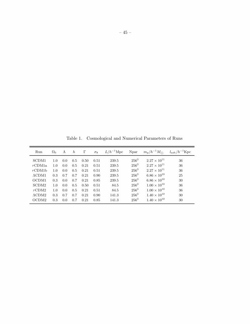
– 45 –

Table 1. Cosmological and Numerical Parameters of Runs

Run Ω0 Λ h Γ σ8 L/h−1Mpc Npar mp/h−1M⊙ lsoft/h−1Kpc

SCDM1 1.0 0.0 0.5 0.50 0.51 239.5 2563 2.27 × 1011 36

τCDM1a 1.0 0.0 0.5 0.21 0.51 239.5 2563 2.27 × 1011 36

τCDM1b 1.0 0.0 0.5 0.21 0.51 239.5 2563 2.27 × 1011 36

ΛCDM1 0.3 0.7 0.7 0.21 0.90 239.5 2563 6.86 × 1010 25

OCDM1 0.3 0.0 0.7 0.21 0.85 239.5 2563 6.86 × 1010 30

SCDM2 1.0 0.0 0.5 0.50 0.51 84.5 2563 1.00 × 1010 36

τCDM2 1.0 0.0 0.5 0.21 0.51 84.5 2563 1.00 × 1010 36

ΛCDM2 0.3 0.7 0.7 0.21 0.90 141.3 2563 1.40 × 1010 30

OCDM2 0.3 0.0 0.7 0.21 0.85 141.3 2563 1.40 × 1010 30

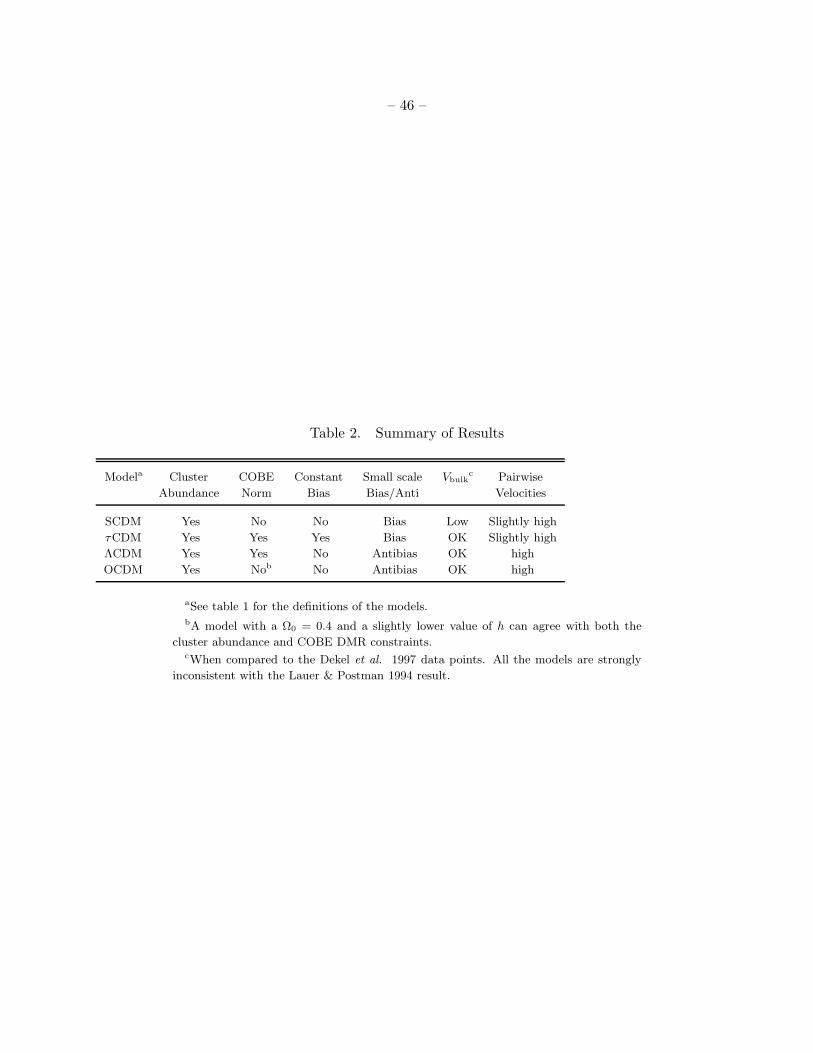
– 46 –

Table 2. Summary of Results

Modela Cluster COBE Constant Small scale Vbulkc Pairwise

Abundance Norm Bias Bias/Anti Velocities

SCDM Yes No No Bias Low Slightly high

τCDM Yes Yes Yes Bias OK Slightly high

ΛCDM Yes Yes No Antibias OK high

OCDM Yes Nob No Antibias OK high

aSee table 1 for the definitions of the models.bA model with a Ω0 = 0.4 and a slightly lower value of h can agree with both the

cluster abundance and COBE DMR constraints.cWhen compared to the Dekel et al. 1997 data points. All the models are strongly

inconsistent with the Lauer & Postman 1994 result.