arX

iv:g

r-qc

/040

4018

v2 3

Sep

200

4

Background Independent Quantum Gravity:

A Status Report

Abhay Ashtekar1,3,4, Jerzy Lewandowski2,1,3,4

1. Physics Department, 104 Davey, Penn State, University Park, PA 16802, USA

2. Institute of Theoretical Physics, University of Warsaw, ul. Hoza 69, 00-681 Warsaw, Poland

3. Max Planck Institut fur Gravitationally, Albert Einstein Institut, 14476 Golm, Germany

4. Erwin Schrodinger Institute, Boltzmanngasse 9, 1090 Vienna, Austria

Abstract

The goal of this article is to present an introduction to loop quantum grav-

ity —a background independent, non-perturbative approach to the problem

of unification of general relativity and quantum physics, based on a quantum

theory of geometry. Our presentation is pedagogical. Thus, in addition to

providing a bird’s eye view of the present status of the subject, the article

should also serve as a vehicle to enter the field and explore it in detail. To

aid non-experts, very little is assumed beyond elements of general relativity,

gauge theories and quantum field theory. While the article is essentially self-

contained, the emphasis is on communicating the underlying ideas and the

significance of results rather than on presenting systematic derivations and

detailed proofs. (These can be found in the listed references.) The subject

can be approached in different ways. We have chosen one which is deeply

rooted in well established physics and also has sufficient mathematical preci-

sion to ensure that there are no hidden infinities. In order to keep the article

to a reasonable size, and to avoid overwhelming non-experts, we have had to

leave out several interesting topics, results and viewpoints; this is meant to

be an introduction to the subject rather than an exhaustive review of it.

Pacs 04.60Pp, 04.60.Ds, 04.60.Nc, 03.65.Sq

1

Contents

I Introduction 5

A The viewpoint . . . . . . . . . . . . . . . . . . . . . . . . . . . . . . . . . 5B Physical questions of quantum gravity . . . . . . . . . . . . . . . . . . . . 6C Organization . . . . . . . . . . . . . . . . . . . . . . . . . . . . . . . . . . 8

II Connection theories of gravity 9

A Holst’s modification of the Palatini action . . . . . . . . . . . . . . . . . . 10B Riemannian signature and half flat connections . . . . . . . . . . . . . . . 13

1 Preliminaries . . . . . . . . . . . . . . . . . . . . . . . . . . . . . . . . 132 The Legendre transform . . . . . . . . . . . . . . . . . . . . . . . . . . 143 The Hamiltonian framework . . . . . . . . . . . . . . . . . . . . . . . . 15

C Generic real value of γ . . . . . . . . . . . . . . . . . . . . . . . . . . . . . 161 Preliminaries . . . . . . . . . . . . . . . . . . . . . . . . . . . . . . . . 162 The Legendre transform . . . . . . . . . . . . . . . . . . . . . . . . . . 173 Hamiltonian theory . . . . . . . . . . . . . . . . . . . . . . . . . . . . 18

III Quantization strategy 20

A Scalar field theories . . . . . . . . . . . . . . . . . . . . . . . . . . . . . . 21B Theories of Connections . . . . . . . . . . . . . . . . . . . . . . . . . . . . 22

IV Quantum theories of connections: background independent kinematics 24

A Quantum mechanics on a compact Lie group G . . . . . . . . . . . . . . . 251 Phase space . . . . . . . . . . . . . . . . . . . . . . . . . . . . . . . . . 252 Quantization . . . . . . . . . . . . . . . . . . . . . . . . . . . . . . . . 263 Spin states. . . . . . . . . . . . . . . . . . . . . . . . . . . . . . . . . . 27

B Connections on a graph . . . . . . . . . . . . . . . . . . . . . . . . . . . . 271 Spaces of connections on a graph . . . . . . . . . . . . . . . . . . . . . 282 Quantum theory . . . . . . . . . . . . . . . . . . . . . . . . . . . . . . 293 Generalized spin network decomposition . . . . . . . . . . . . . . . . . 30

C Connections on M . . . . . . . . . . . . . . . . . . . . . . . . . . . . . . . 321 The classical phase space . . . . . . . . . . . . . . . . . . . . . . . . . 322 Quantum configuration space A and Hilbert space H . . . . . . . . . . 353 Generalized spin networks . . . . . . . . . . . . . . . . . . . . . . . . . 374 Elementary quantum operators . . . . . . . . . . . . . . . . . . . . . . 385 Gauge and Diffeomorphism symmetries . . . . . . . . . . . . . . . . . 39

V Quantum Riemannian geometry 42

A Area operators . . . . . . . . . . . . . . . . . . . . . . . . . . . . . . . . . 421 Regularization . . . . . . . . . . . . . . . . . . . . . . . . . . . . . . . 422 Properties of area operators . . . . . . . . . . . . . . . . . . . . . . . . 443 The gauge invariant subspace . . . . . . . . . . . . . . . . . . . . . . 45

B Volume operators . . . . . . . . . . . . . . . . . . . . . . . . . . . . . . . 471 Regularization . . . . . . . . . . . . . . . . . . . . . . . . . . . . . . . 47

2

2 Properties of volume operators . . . . . . . . . . . . . . . . . . . . . . 493 ‘External’ regularization . . . . . . . . . . . . . . . . . . . . . . . . . . 50

VI Quantum dynamics 51

A The Gauss constraint . . . . . . . . . . . . . . . . . . . . . . . . . . . . . 52B The diffeomorphism constraint . . . . . . . . . . . . . . . . . . . . . . . . 53

1 Strategy . . . . . . . . . . . . . . . . . . . . . . . . . . . . . . . . . . . 532 Physical states . . . . . . . . . . . . . . . . . . . . . . . . . . . . . . . 54

C The Scalar Constraint . . . . . . . . . . . . . . . . . . . . . . . . . . . . . 571 Regulated classical expression . . . . . . . . . . . . . . . . . . . . . . . 572 The quantum scalar constraint . . . . . . . . . . . . . . . . . . . . . . 613 Solutions to the scalar constraint . . . . . . . . . . . . . . . . . . . . . 64

VII Applications of quantum geometry: Quantum cosmology 67

A Phase space . . . . . . . . . . . . . . . . . . . . . . . . . . . . . . . . . . . 67B Quantization: kinematics . . . . . . . . . . . . . . . . . . . . . . . . . . . 69

1 Elementary variables . . . . . . . . . . . . . . . . . . . . . . . . . . . . 692 Representation of the algebra of elementary variables . . . . . . . . . . 70

C Triad operator . . . . . . . . . . . . . . . . . . . . . . . . . . . . . . . . . 72D Quantum dynamics: The Hamiltonian constraint . . . . . . . . . . . . . . 74

1 The constraint operator . . . . . . . . . . . . . . . . . . . . . . . . . . 742 Physical states . . . . . . . . . . . . . . . . . . . . . . . . . . . . . . . 77

VIII Applications: Quantum geometry of isolated horizons and black hole

entropy 79

A Isolated horizons . . . . . . . . . . . . . . . . . . . . . . . . . . . . . . . . 80B Type I isolated horizons: Quantum theory . . . . . . . . . . . . . . . . . . 82

1 Hamiltonian framework . . . . . . . . . . . . . . . . . . . . . . . . . . 822 Quantum horizon geometry . . . . . . . . . . . . . . . . . . . . . . . . 833 Entropy: Counting surface states . . . . . . . . . . . . . . . . . . . . . 87

C Non-minimal couplings and type II horizons . . . . . . . . . . . . . . . . . 891 Non-minimal couplings . . . . . . . . . . . . . . . . . . . . . . . . . . 892 Inclusion of distortion and rotation . . . . . . . . . . . . . . . . . . . . 91

IX Current Directions 93

A Low energy physics . . . . . . . . . . . . . . . . . . . . . . . . . . . . . . 931 Quantum mechanics of particles . . . . . . . . . . . . . . . . . . . . . 942 The Maxwell field and linearized gravity . . . . . . . . . . . . . . . . . 953 Quantum geometry . . . . . . . . . . . . . . . . . . . . . . . . . . . . 97

B Spin foams . . . . . . . . . . . . . . . . . . . . . . . . . . . . . . . . . . . 100

X Outlook 102

APPENDIXES 106

3

A Inclusion of Matter fields:

The Einstein-Maxwell theory 106

1 Classical framework . . . . . . . . . . . . . . . . . . . . . . . . . . . . . . 1062 Quantum kinematics . . . . . . . . . . . . . . . . . . . . . . . . . . . . . . 1073 The quantum constraints . . . . . . . . . . . . . . . . . . . . . . . . . . . 108

a Regularization of the 3-geometry part in CMax(N) . . . . . . . . . . . . 108b Quantization of the electric part of CMax(N) . . . . . . . . . . . . . . . 109c Quantization of the magnetic part . . . . . . . . . . . . . . . . . . . . 110d summary . . . . . . . . . . . . . . . . . . . . . . . . . . . . . . . . . . 111

B List of Symbols 113

4

I. INTRODUCTION

This section is divided into three parts. In the first, we outline the general, conceptualviewpoint that underlies loop quantum gravity; in the second, we recall some of the centralphysical problems of quantum gravity; and in the third, we summarize the progress that hasbeen made in addressing these issues and sketch the organization of the paper.

A. The viewpoint

In this approach, one takes the central lesson of general relativity seriously: gravityis geometry whence, in a fundamental theory, there should be no background metric. Inquantum gravity, geometry and matter should both be ‘born quantum mechanically’. Thus,in contrast to approaches developed by particle physicists, one does not begin with quantummatter on a background geometry and use perturbation theory to incorporate quantumeffects of gravity. There is a manifold but no metric, or indeed any other fields, in thebackground.1

At the classical level, Riemannian geometry provides the appropriate mathematical lan-guage to formulate the physical, kinematical notions as well as the final dynamical equationsof modern gravitational theories. This role is now taken by quantum Riemannian geometry,discussed in sections IV and V. In the classical domain, general relativity stands out as thebest available theory of gravity, some of whose predictions have been tested to an amazingaccuracy, surpassing even the legendary tests of quantum electrodynamics. Therefore, it isnatural to ask: Does quantum general relativity, coupled to suitable matter (or supergravity,its supersymmetric generalization) exist as a consistent theory non-perturbatively?

In the particle physics circles, the answer is often assumed to be in the negative, notbecause there is concrete evidence against non-perturbative quantum gravity, but becauseof an analogy to the theory of weak interactions. There, one first had a 4-point interactionmodel due to Fermi which works quite well at low energies but which fails to be renormal-izable. Progress occurred not by looking for non-perturbative formulations of the Fermimodel but by replacing the model with the Glashow-Salam-Weinberg renormalizable theoryof electro-weak interactions, in which the 4-point interaction is replaced by W± and Z prop-agators. It is often assumed that perturbative non-renormalizability of quantum generalrelativity points in a similar direction. However this argument overlooks the crucial factthat, in the case of general relativity, there is a qualitatively new element. Perturbativetreatments pre-suppose that space-time can be assumed to be a continuum at all scales ofinterest to physics under consideration. This appears to be a safe assumption in theories ofelectro-weak and strong interactions. In the gravitational case, on the other hand, the scaleof interest is given by the Planck length ℓPl and there is no physical basis to pre-suppose

1In 2+1 dimensions, although one begins in a completely analogous fashion, in the final picture

one can get rid of the background manifold as well. Thus, the fundamental theory can be for-

mulated combinatorially [2,35]. To achieve this goal in 3+1 dimensions, one needs a much better

understanding of the theory of (intersecting) knots in 3 dimensions.

5

that the continuum picture should be valid down to that scale. The failure of the stan-dard perturbative treatments may be largely due to this grossly incorrect assumption anda non-perturbative treatment which correctly incorporates the physical micro-structure ofgeometry may well be free of these inconsistencies.

Note that, even if quantum general relativity did exist as a mathematically consistenttheory, there is no a priori reason to assume that it would be the ‘final’ theory of all knownphysics. In particular, as is the case with classical general relativity, while requirements ofbackground independence and general covariance do restrict the form of interactions betweengravity and matter fields and among matter fields themselves, the theory would not have abuilt-in principle which determines these interactions. Put differently, such a theory wouldnot be a satisfactory candidate for unification of all known forces. However, just as generalrelativity has had powerful implications in spite of this limitation in the classical domain,quantum general relativity should have qualitatively new predictions, pushing further theexisting frontiers of physics. Indeed, unification does not appear to be an essential criterionfor usefulness of a theory even in other interactions. QCD, for example, is a powerful theoryeven though it does not unify strong interactions with electro-weak ones. Furthermore, thefact that we do not yet have a viable candidate for the grand unified theory does not makeQCD any less useful.

Finally, the quantum theory of geometry provides powerful tools to do quantum physicsin absence of a background space-time. Being kinematical, it is not rigidly tied to generalrelativity (or supergravity) and may well be useful also in other approaches to quantumgravity.

B. Physical questions of quantum gravity

Approaches to quantum gravity face two types of issues: Problems that are ‘internal’ toindividual approaches and problems that any approach must face. Examples of the formerare: Incorporation of physical —rather than half flat— gravitational fields in twistor theory;mechanisms for breaking of supersymmetry and dimensional reduction in string theory; andissues of space-time covariance in the canonical approach. In this sub-section, we will focuson the second type of issues by recalling some of the long standing issues that any satisfactoryquantum theory of gravity should address.

• Big-Bang and other singularities : It is widely believed that the prediction of a sin-gularity, such as the big-bang of classical general relativity, is primarily a signal that thephysical theory has been pushed beyond the domain of its validity. A key question to anyquantum gravity theory, then, is: What replaces the big-bang? Are the classical geometryand the continuum picture only approximations, analogous to the ‘mean (magnetization)field’ of ferro-magnets? If so, what are the microscopic constituents? What is the space-time analog of a Heisenberg quantum model of a ferro-magnet? When formulated in termsof these fundamental constituents, is the evolution of the quantum state of the universefree of singularities? General relativity predicts that the space-time curvature must growunboundedly as we approach the big-bang or the big-crunch but we expect the quantumeffects, ignored by general relativity, to intervene, making quantum gravity indispensablebefore infinite curvatures are reached. If so, what is the upper bound on curvature? How

6

close to the singularity can we ‘trust’ classical general relativity? What can we say about the‘initial conditions’, i.e., the quantum state of geometry and matter that correctly describesthe big-bang? If they have to be imposed externally, is there a physical guiding principle?

• Black holes: In the early seventies, using imaginative thought experiments, Bekenstein[118] argued that black holes must carry an entropy proportional to their area. About thesame time, Bardeen, Carter and Hawking (BCH) showed that black holes in equilibrium obeytwo basic laws, which have the same form as the zeroth and the first laws of thermodynamics,provided one equates the black hole surface gravity κ to some multiple of the temperature Tin thermodynamics and the horizon area ahor to a corresponding multiple of the entropy S[119]. However, at first this similarity was thought to be only a formal analogy because theBCH analysis was based on classical general relativity and simple dimensional considerationsshow that the proportionality factors must involve Planck’s constant ~. Two years later,using quantum field theory on a black hole background space-time, Hawking [120] showedthat black holes in fact radiate quantum mechanically as though they are black bodies attemperature T = ~κ/2π. Using the analogy with the first law, one can then conclude thatthe black hole entropy should be given by SBH = ahor/4G~. This conclusion is striking anddeep because it brings together the three pillars of fundamental physics —general relativity,quantum theory and statistical mechanics. However, the argument itself is a rather hodge-podge mixture of classical and semi-classical ideas, reminiscent of the Bohr theory of atom.A natural question then is: what is the analog of the more fundamental, Pauli-Schrodingertheory of the Hydrogen atom? More precisely, what is the statistical mechanical origin ofblack hole entropy? What is the nature of a quantum black hole and what is the interplaybetween the quantum degrees of freedom responsible for entropy and the exterior curvedgeometry? Can one derive the Hawking effect from first principles of quantum gravity? Isthere an imprint of the classical singularity on the final quantum description, e.g., through‘information loss’?

• Planck scale physics and the low energy world: In general relativity, there is no back-ground metric, no inert stage on which dynamics unfolds. Geometry itself is dynamical.Therefore, as indicated above, one expects that a fully satisfactory quantum gravity theorywould also be free of a background space-time geometry. However, of necessity, a back-ground independent description must use physical concepts and mathematical tools that arequite different from those of the familiar, low energy physics. A major challenge then is toshow that this low energy description does arise from the pristine, Planckian world in anappropriate sense, bridging the vast gap of some 16 orders of magnitude in the energy scale.In this ‘top-down’ approach, does the fundamental theory admit a ‘sufficient number’ ofsemi-classical states? Do these semi-classical sectors provide enough of a background geom-etry to anchor low energy physics? Can one recover the familiar description? Furthermore,can one pin point why the standard ‘bottom-up’ perturbative approach fails? That is, whatis the essential feature which makes the fundamental description mathematically coherentbut is absent in the standard perturbative quantum gravity?

There are of course many more challenges: the issue of time, of measurement theory andthe associated questions of interpretation of the quantum framework, the issue of diffeomor-phism invariant observables and practical methods of computing their properties, practicalmethods of computing time evolution and S-matrices, exploration of the role of topologyand topology change, etc etc. However, it is our view that the three issues discussed in de-

7

tail are more basic from a physical viewpoint because they are rooted in general conceptualquestions that are largely independent of the specific approach being pursued; indeed theyhave been with us longer than any of the current leading approaches.

C. Organization

In recent years, a number of these fundamental physical issues were addressed in loopquantum gravity. These include: i) A natural resolution of the big-bang singularity in ho-mogeneous, isotropic quantum cosmology [103-117]; ii) A statistical mechanical derivationof the horizon entropy, encompassing astrophysically interesting black holes as well as cos-mological horizons [122-141]; and, iii) The introduction of semi-classical techniques to makecontact between the background independent, non-perturbative theory and the perturba-tive, low energy physics in Minkowski space [142-160]. In addition, advances have beenmade on the mathematical physics front. In particular, these include: iv) A demonstrationthat all Riemannian geometric operators have discrete eigenvalues, implying that the space-time continuum is only an approximation [65-80]; v) A systematic formulation of quantumEinstein equations in the canonical approach [85-102]; and, vi) The development of spin-foam models which provide background independent path integral formulations of quantumgravity [161-173]. These developments are also significant. For example, in contrast to v),quantum Einstein’s equations are yet to be given a precise mathematical meaning in quan-tum geometrodynamics —a canonical approach that predates loop quantum gravity by twodecades or so— because the products of operators involved are divergent.

All these advances spring from a detailed quantum theory of geometry that was sys-tematically developed in the mid-nineties. This theory is, in turn, an outgrowth of twodevelopments: a) Formulation of general relativity (and supergravity) as a dynamical the-ory of connections, with the same phase space as in Yang-Mills theories [12-16]; and, b)heuristic but highly influential treatments of quantum theories of connections in terms ofloops [33-38].2 In this review, we will first provide a brief but self-contained and pedagogicalintroduction to quantum geometry and then discuss its applications to problems mentionedabove.

The article is organized as follows. In section II we recall connection formulations ofgeneral relativity. (Readers who are primarily interested in quantum geometry rather thandynamical issues of general relativity may skip this section in the first reading.) The nextfour sections present the basics of quantum theory. In section III we summarize the overallstrategy used in the construction of quantum kinematics; in section IV, we discuss back-ground independent formulations of general quantum theories of connections; in section V,the basics of quantum Riemannian geometry and in section VI the basics of quantum dy-namics. These sections are self-contained and the reader is referred to the original papersonly for certain proofs, technical subtleties and details that are interesting in their own right

2This is the origin of the name ‘loop quantum gravity’. Even though loops play no essential role

in the theory now, for historical reasons, this name is widely used. The current framework is based

on graphs introduced in [40–42].

8

but not essential to follow the general approach. Sections VII-IX are devoted to applica-tions of quantum geometry and a summary of current directions, where the treatment isless pedagogical: while the main ideas are spelled out, the reader will have to go through atleast some of the original papers to get a thorough working knowledge. Section X containsa summary and the outlook.

For simplicity, most of the discussion in the main body of the review is focussed on thegravitational field. There is a large body of work on coupling of gauge, fermionic and scalarfields to gravity where the quantum nature of underlying geometry modifies the physics ofmatter fields in important ways. Appendix A illustrates these issues using the Einstein-Maxwell theory as an example. Appendix B contains a list of symbols which are frequentlyused in the review.

For a much more detailed review, at the level of a monograph, see, [9]. Less pedagogicaloverviews, at the level of plenary lectures in conferences, can be found in [6,8].

II. CONNECTION THEORIES OF GRAVITY

General relativity is usually presented as a theory of metrics. However, it can also berecast as a dynamical theory of connections.3 Such a reformulation brings general relativitycloser to gauge theories which describe the other three fundamental forces of Nature inthe sense that, in the Hamiltonian framework, all theories now share the same kinematics.The difference, of course, lies in dynamics. In particular, while dynamics of gauge theoriesof other interactions requires a background geometry, that of general relativity does not.Nonetheless, by a suitable modification, one can adapt quantization techniques used in gaugetheories to general relativity. We will see in sections IV,V and VI that this strategy enablesone to resolve the functional analytic difficulties which have prevented ‘geometrodynamical’approaches to quantum gravity, based on metrics, to progress beyond a formal level.

In this section, we will present a self-contained introduction to connection formulationsof general relativity. However, we will not follow a chronological approach but focus insteadonly on those aspects which are needed in subsequent sections. For a discussion of otherissues, see [2, 12-23].

Our conventions are as follows. M will denote the 4-dimensional space-time manifoldwhich we will assume to be topologically M × R, equipped with a fixed orientation. Forsimplicity, in this section we will assume that M is an oriented, compact 3-manifold with-out boundary. (Modifications required to incorporate asymptotic flatness can be found in[2] and those needed to allow an isolated horizon as an inner boundary can be found in[133,134].) For tensor fields (possibly with internal indices), we will use Penrose’s abstractindex notation. The space-time metric will be denoted by gµν and will have signature -,+,+,+ (or, occasionally, +,+,+,+. In the Lorentzian case, space-time will be assumed tobe time-orientable.) The torsion-free derivative operator compatible with gµν will be denoted

3Indeed, in the late forties both Einstein and Schrodinger had recast general relativity as a theory

of connections. However, the resulting theory was rather complicated because they used the Levi-

Civita connection. Theory simplifies if one uses spin-connections instead.

9

by ∇ and its curvature tensors will be defined via RαβγδKδ = 2∇[α∇β]Kγ; Rαβ = Rαβγ

β;and R = gαβRαβ. For the tetrad formalism, we fix a 4-dimensional vector space V equippedwith a fixed metric ηIJ of signature -,+,+,+ (or +,+,+,+), which will serve as the ‘internalspace’. Orthonormal co-tetrads will be denoted by eI

α; thus gαβ = ηIJeIαe

Jβ . In the passage

to the Hamiltonian theory, the metric on a space-like Cauchy surface M will be denoted byqab and the spatial co-triads will be denoted by ei

a. Finally, we will often set k = 8πG whereG is Newton’s constant. Due to space limitation, we will focus just on the gravitational partof the action and phase space. For inclusion of matter, see e.g., [16,133]; for extension tosupergravity, see, e.g., [17]; and for ideas on extension to higher dimensions, see [25].

A. Holst’s modification of the Palatini action

In the Palatini framework, the basic gravitational variables constitute a pair (eµI , ωµ

IJ)

of 1-form fields on M taking values, respectively, in V and in the Lie algebra so(η) of thegroup SO(η) of the linear transformations of V preserving ηIJ . Because of our topologi-cal assumptions, the co-frame fields eµ

I are defined globally; they provide an isomorphismbetween TxM and V at each x ∈ M. The action is given by

S(P )(e, ω) =1

4k

∫

M

ǫIJKL eI ∧ eJ ∧ ΩKL (2.1)

where ǫIJKL is an alternating tensor on V compatible with ηIJ such that the orientation ofǫαβγδ = ǫIJKL e

Iαe

Jβe

Kγ e

Lδ agrees with the one we fixed on M and

Ω := dω + ω ∧ ω, (2.2)

is the curvature of the connection 1-form ωµIJ . The co-frame eI

µ determines a space-timemetric gµν = ηIJ e

Iµe

Jν . Thus, in contrast to the more familiar Einstein-Hilbert action, S(P )

depends on an additional variable, the connection ωIJµ . However, the equation of motion

obtained by varying the action with respect to the connection implies that ωIJµ is in fact

completely determined by the co-frame:

de+ ω ∧ e = 0. (2.3)

If we now restrict ourselves to histories on which the connection is so determined, S(P )

reduces to the familiar Einstein-Hilbert action:

S(P )(e, ω(e)) =1

2k

∫

M

d4x√

| det g|R . (2.4)

where R is the scalar curvature of gµν . Therefore, the equation of motion for the metric isthe same as that of the Einstein-Hilbert action.

The action S(P ) is invariant under diffeomorphisms of M as well as local SO(η) trans-formations

(e, ω) 7→ (e′, ω′) = (b−1e, b−1ωb+ b−1db) . (2.5)

10

It is straightforward but rather tedious to perform a Legendre transform of this actionand pass to a Hamiltonian theory [18]. It turns out that the theory has certain secondclass constraints and, when they are solved, one is led to a triad version of the standardHamiltonian theory of geometrodynamics; all reference to connection-dynamics is lost. Thiscan be remedied using the following observation: there exists another invariant, constructedfrom the pair (e, ω), with the remarkable property that its addition to the action does notchange equations of motion. The modified action, discussed by Holst [21], is given by4:

S(H)(e, ω) = S(P )(e, ω) − 1

2kγ

∫

M

eI ∧ eJ ∧ ΩIJ (2.6)

where γ is an arbitrary but fixed number, called the Barbero-Immirzi parameter. For ap-plications to quantum theory, it is important to note that γ can not be zero. The purposeof this section is to analyze this action and the Hamiltonian theory emerging from it. Insections IIB and IIC we will show that the Hamiltonian theory can be naturally interpretedas a background independent, dynamical theory of connections.

Recall that, in Yang-Mills theories, one can also add a ‘topological term’ to the actionwhich does not change the classical equations of motion because its integrand can be re-expressed as an exterior derivative of a three-form. In the present case, while the extra termis not of topological origin, because of the first Bianchi identity it vanishes identically onhistories on which (2.3) holds. Therefore the situation is similar in the two theories in somerespects: in both cases, the addition of the term does not change the classical equations ofmotion and it induces a canonical transformation on the classical phase space which failsto be unitarily implementable in the quantum theory. Consequently, the parameter γ is inmany ways analogous to the well-known θ parameter in the Yang-Mills theory [83,84]. Justas the quantum theory has inequivalent θ-sectors in the Yang-Mills case, it has inequivalentγ-sectors in the gravitational case.

We will conclude this preliminary discussion by exhibiting the symplectic structure inthe covariant phase space formulation. Here the phase space Γcov is taken to be the space of(suitably regular) solutions to the field equations on M. To define the symplectic structure,one follows the following general procedure. Denote by δ ≡ (δe, δω) tangent vectors in thespace of histories. Since field equations are satisfied on Γcov, the change in the Lagrangian4-form L4 under a variation along δ is for the form

(δL4)|Γcov = dL3(δ)

for some 3-form L3 on M which depends linearly on δ. One can now define a 1-form Θ

on the space of histories via: Θ(δ) :=∫

ML3(δ). The symplectic structure Ω is simply the

pull-back to Γcov of the curl of Θ on the space of histories. In our case, δL(H) is given by

δL(H) = − 1

2γkd[eI ∧ eJ ∧ δ

(ωIJ − γ

2ǫIJKLω

KL)].

4This modification was strongly motivated by the very considerable work on the framework based

on(anti-)self-dual connections in the preceding decade (see e.g. [2]) particularly by the discovery of

an action for general relativity using these variables [14]. Also, our presentation contains several

new elements which, to our knowledge, have not appeared in the literature before.

11

whence the symplectic structure is given by:

Ω(δ1, δ2) = − 1

kγ

∫

M

[δ[1(e

I ∧ eJ )]∧[δ2](ωIJ − γ

2ǫIJKLω

KL)]

(2.7)

for all tangent vectors δ1 and δ2 to Γcov. From general considerations, it follows that thevalue of the integral is independent of the specific choice of a Cauchy surface M made in itsevaluation.

Using the fact that the tangent vectors to Γcov must, in particular, satisfy the linearizedversion of (2.3) it is easy to verify that the γ-dependent term in (2.7) vanishes identically:Not only is Γcov independent of the value of γ (see footnote 5) but so is the symplecticstructure Ω on it. As is clear from (2.7), the momentum conjugate to eI ∧ eJ , on the otherhand, does depend on the choice of γ. Thus, as noted above, like the θ term in the Yang-Millstheory, the γ term in (2.6) only induces a canonical transformation on the phase space.

In effect the canonical transformation is induced by the map

XIJ 7→ 1

2

(XIJ − γ

2ǫIJKLX

KL)

on so(η). It is easy to verify that this map is a vector space isomorphism on so(η) exceptwhen

γ2 = σ := sgn(det η) ,

the sign of the determinant of the metric tensor ηIJ .5 At these exceptional values of γ,the map is a projection onto the subspace of so(η) corresponding to the eigenvalue −γσ ofthe Hodge-dual operator ⋆ : XIJ 7→ 1

2ǫIJ

KLXKL. Furthermore, in this case the map is aLie algebra homomorphism. In the Riemannian case (when η has signature +,+,+,+) thisoccurs for γ = ±1 while in the Lorentzian case (when η has signature -,+,+,+) it occursfor γ = ±i. In all these exceptional cases the theory has a richer geometrical structure. Inparticular, the combination 1

2(ωIJ − γ ⋆ωIJ) that occurs in the symplectic structure is again

a (half-flat) connection.Chronologically, the background independent approach to quantum gravity summarized

in this review originated from a reformulation of general relativity in terms of these half-flatconnections [12,13]. It turns out that all equations in the classical theory simplify consid-erably and underlying structures become more transparent in these variables. They arealso closely related to Penrose’s non-linear gravitons [31] and Newman’s H-space construc-tions [32]. In the Riemannian signature, one can continue to use these variables also in thequantum theory. In the Lorentzian case, on the other hand, the half-flat connections take

5As a result, for generic values of γ, the equation of motion for the connection resulting from

variation of S(H) with respect to ωIJµ is again (2.3). Hence the space of solutions obtained by varying

S(H) is the same as that obtained by varying S(P ). For the exceptional values, this equation says

that the (anti-) self dual part of ωIJµ equals the (anti-) self dual part of the connection compatible

with the co-frame eIµ. However, it is again true that the spaces of solutions obtained by extremizing

S(H) and S(P ) are the same [2].

12

values in the Lie algebra of non-compact groups and functional analysis on spaces of suchconnections is still not sufficiently well-developed to carry out constructions required in thequantum theory. Therefore, in the Lorentzian case, most progress has occurred by workingin sectors with real values of γ where, as we will see, one can work connections with compactstructure groups.

In section IIB we will summarize the situation with half-flat connections in the Rie-mannian case and in section IIC we will discuss the Lorentzian theory using real valued γsectors.

B. Riemannian signature and half flat connections

1. Preliminaries

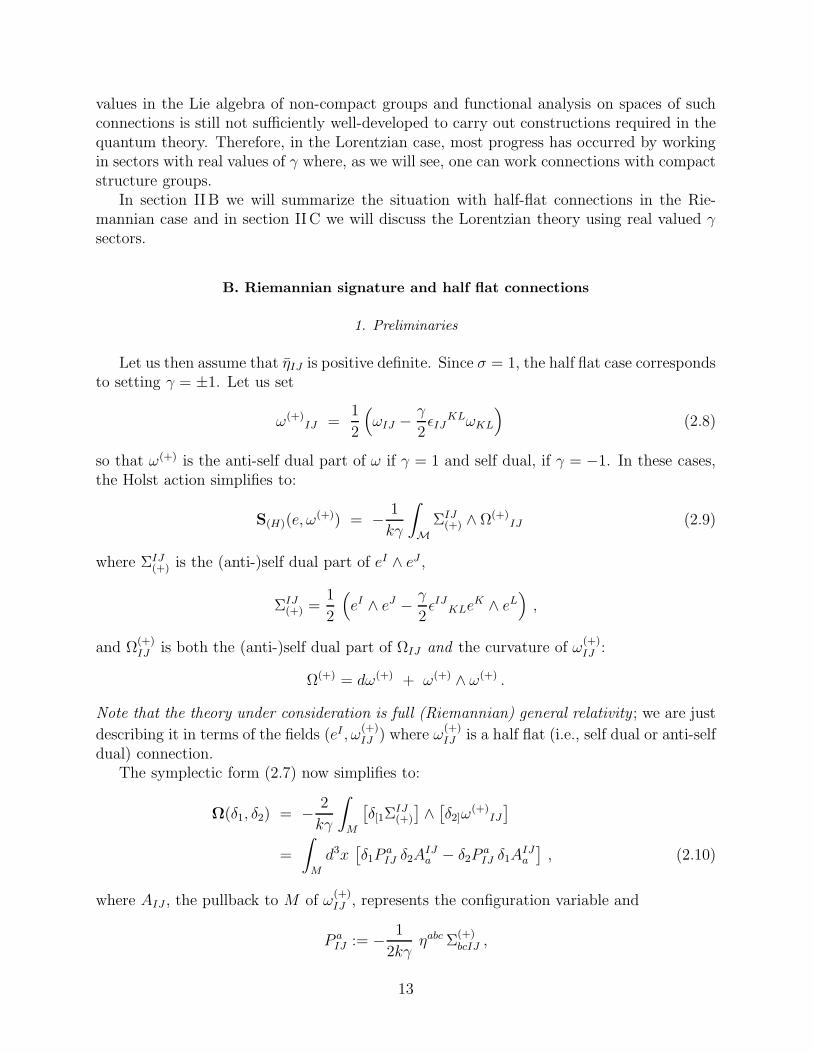
Let us then assume that ηIJ is positive definite. Since σ = 1, the half flat case correspondsto setting γ = ±1. Let us set

ω(+)IJ =

1

2

(ωIJ − γ

2ǫIJ

KLωKL

)(2.8)

so that ω(+) is the anti-self dual part of ω if γ = 1 and self dual, if γ = −1. In these cases,the Holst action simplifies to:

S(H)(e, ω(+)) = − 1

kγ

∫

M

ΣIJ(+) ∧ Ω(+)

IJ (2.9)

where ΣIJ(+) is the (anti-)self dual part of eI ∧ eJ ,

ΣIJ(+) =

1

2

(eI ∧ eJ − γ

2ǫIJ

KLeK ∧ eL

),

and Ω(+)IJ is both the (anti-)self dual part of ΩIJ and the curvature of ω

(+)IJ :

Ω(+) = dω(+) + ω(+) ∧ ω(+) .

Note that the theory under consideration is full (Riemannian) general relativity ; we are just

describing it in terms of the fields (eI , ω(+)IJ ) where ω

(+)IJ is a half flat (i.e., self dual or anti-self

dual) connection.The symplectic form (2.7) now simplifies to:

Ω(δ1, δ2) = − 2

kγ

∫

M

[δ[1Σ

IJ(+)

]∧[δ2]ω

(+)IJ

]

=

∫

M

d3x[δ1P

aIJ δ2A

IJa − δ2P

aIJ δ1A

IJa

], (2.10)

where AIJ , the pullback to M of ω(+)IJ , represents the configuration variable and

P aIJ := − 1

2kγηabc Σ

(+)bcIJ ,

13

its canonically conjugate momentum. Here and in what follows ηabc will denote the metricindependent Levi-Civita density on M whose orientation is the same as that of the fixedorientation on M . Hence P a

IJ is a pseudo vector density of the weight 1 on M .6

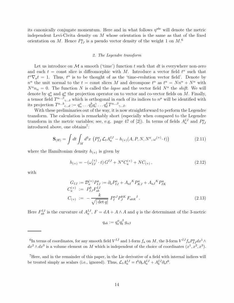
2. The Legendre transform

Let us introduce on M a smooth (‘time’) function t such that dt is everywhere non-zeroand each t = const slice is diffeomorphic with M . Introduce a vector field tα such thattα∇at = 1. Thus, tα is to be thought of as the ‘time-evolution vector field’. Denote bynα the unit normal to the t = const slices M and decompose tα as tα = Nnα + Nα withNαnα = 0. The function N is called the lapse and the vector field Nα the shift. We willdenote by qa

α and qαa the projection operator on to vector and co-vector fields on M . Finally,

a tensor field T α...βγ...δ which is orthogonal in each of its indices to nµ will be identified with

its projection T a...bc...d := qa

α . . . qbβq

γc . . . q

δd T

α...βγ...δ.

With these preliminaries out of the way, it is now straightforward to perform the Legendretransform. The calculation is remarkably short (especially when compared to the Legendretransform in the metric variables; see, e.g. page 47 of [2]). In terms of fields AIJ

a and P aIJ

introduced above, one obtains7:

S(H) =

∫dt

∫

M

d3x(P a

IJ LtAIJa − h(+)(A,P,N,N

a, ω(+) · t))

(2.11)

where the Hamiltonian density h(+) is given by

h(+) = −(ω(+)IJ · t)GIJ +NaC(+)

a +NC(+) , (2.12)

with

GIJ := D(+)a P a

IJ := ∂aPaIJ + AaI

KP aKJ + AaJ

KP aIK

C(+)a := P b

IJFIJab

C(+) := − k√| det q|

P aI

JP bJ

K FabKI . (2.13)

Here F IJab is the curvature of AIJ

a , F = dA+A∧A and q is the determinant of the 3-metric

qab := qαa q

βb gαβ

6In terms of coordinates, for any smooth field V IJ and 1-form fa on M , the 3-form V IJfaPaIJdx1∧

dx2 ∧ dx3 is a volume element on M which is independent of the choice of coordinates (x1, x2, x3).

7Here, and in the remainder of this paper, in the Lie derivative of a field with internal indices will

be treated simply as scalars (i.e., ignored). Thus, LtAIJa = tb∂bA

IJa + AIJ

b ∂atb.

14

on M . The form of (2.12) confirms that, as suggested by (2.10), we should regard AIJa as

the configuration variable and P aIJ as its momentum. The momentum is related in a simple

way to the 3-metric:

−TrP aP b = P aIJP

bIJ =1

k2(det q) qab ,

Note that ω · t, N and Na are Lagrange multipliers; there are no equations governingthem. The basic dynamical variables are only AIJ

a and P aIJ ; all other dynamical fields are

determined by them. Variation of S(H) with respect to these multipliers yields constraints:

GIJ = 0; C(+)a = 0; and C(+) = 0. (2.14)

As is always the case (in the spatially compact context) for theories without backgroundfields the Hamiltonian is a sum of constraints. Variations of the action with respect to AIJ

a

and P aIJ yield the equations of motion for these basic dynamical fields. The three constraints

(2.13) and these two evolution equations are equivalent to the full set of Einstein’s equations.

3. The Hamiltonian framework

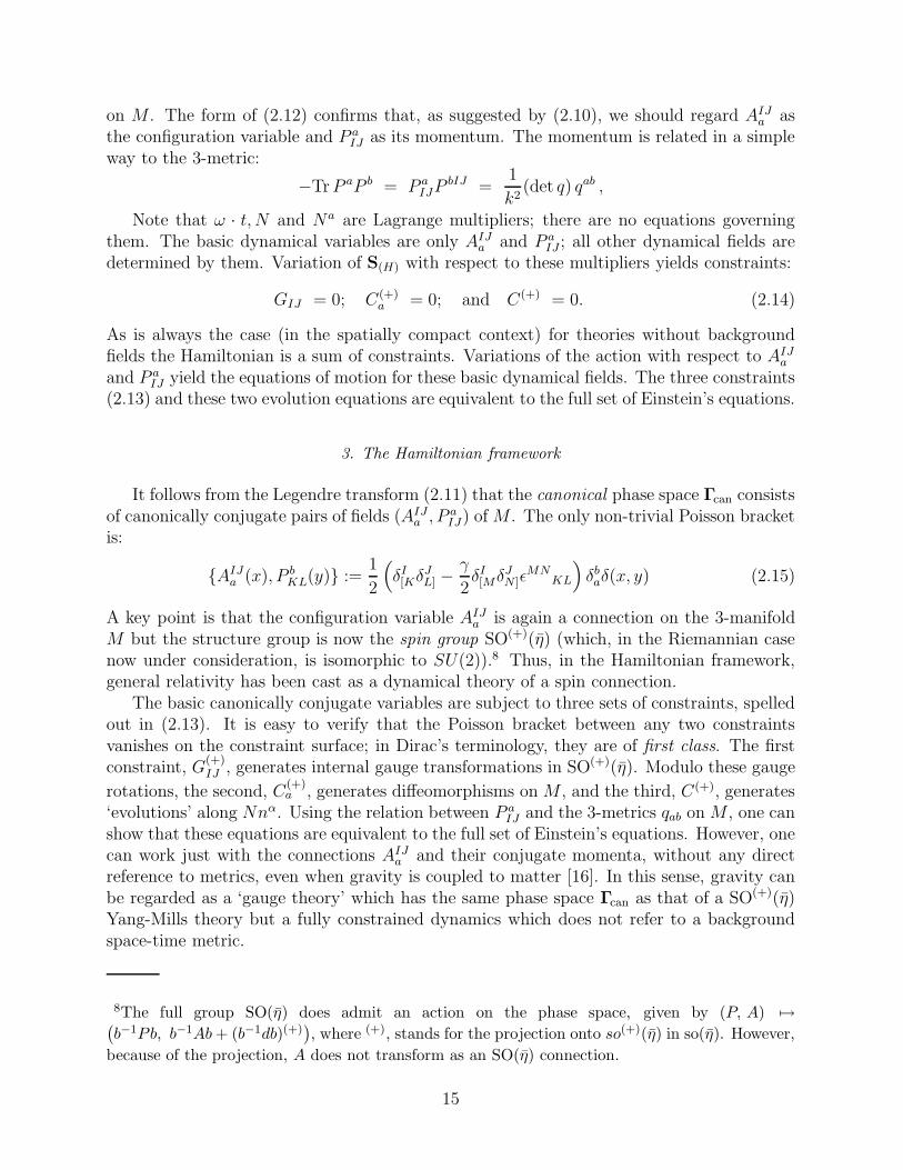
It follows from the Legendre transform (2.11) that the canonical phase space Γcan consistsof canonically conjugate pairs of fields (AIJ

a , PaIJ) of M . The only non-trivial Poisson bracket

is:

AIJa (x), P b

KL(y) :=1

2

(δI[Kδ

JL] −

γ

2δI[Mδ

JN ]ǫ

MNKL

)δbaδ(x, y) (2.15)

A key point is that the configuration variable AIJa is again a connection on the 3-manifold

M but the structure group is now the spin group SO(+)(η) (which, in the Riemannian casenow under consideration, is isomorphic to SU(2)).8 Thus, in the Hamiltonian framework,general relativity has been cast as a dynamical theory of a spin connection.

The basic canonically conjugate variables are subject to three sets of constraints, spelledout in (2.13). It is easy to verify that the Poisson bracket between any two constraintsvanishes on the constraint surface; in Dirac’s terminology, they are of first class. The firstconstraint, G

(+)IJ , generates internal gauge transformations in SO(+)(η). Modulo these gauge

rotations, the second, C(+)a , generates diffeomorphisms on M , and the third, C(+), generates

‘evolutions’ along Nnα. Using the relation between P aIJ and the 3-metrics qab on M , one can

show that these equations are equivalent to the full set of Einstein’s equations. However, onecan work just with the connections AIJ

a and their conjugate momenta, without any directreference to metrics, even when gravity is coupled to matter [16]. In this sense, gravity canbe regarded as a ‘gauge theory’ which has the same phase space Γcan as that of a SO(+)(η)Yang-Mills theory but a fully constrained dynamics which does not refer to a backgroundspace-time metric.

8The full group SO(η) does admit an action on the phase space, given by (P, A) 7→(b−1Pb, b−1Ab + (b−1db)(+)

), where (+), stands for the projection onto so(+)(η) in so(η). However,

because of the projection, A does not transform as an SO(η) connection.

15

C. Generic real value of γ

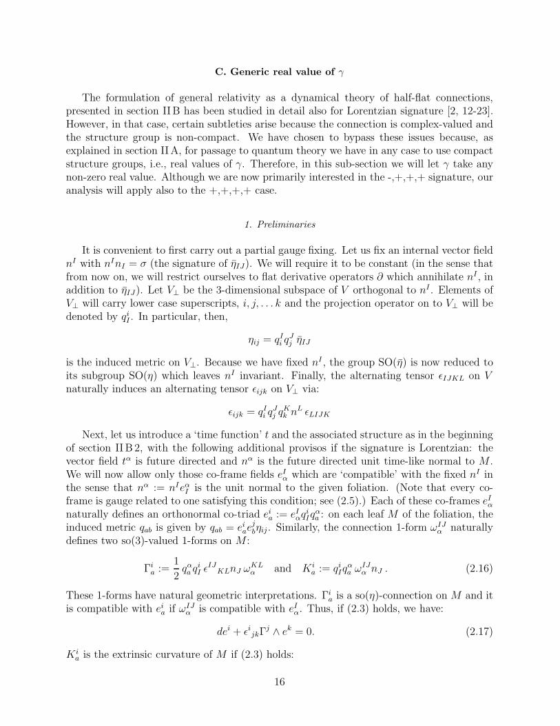
The formulation of general relativity as a dynamical theory of half-flat connections,presented in section IIB has been studied in detail also for Lorentzian signature [2, 12-23].However, in that case, certain subtleties arise because the connection is complex-valued andthe structure group is non-compact. We have chosen to bypass these issues because, asexplained in section IIA, for passage to quantum theory we have in any case to use compactstructure groups, i.e., real values of γ. Therefore, in this sub-section we will let γ take anynon-zero real value. Although we are now primarily interested in the -,+,+,+ signature, ouranalysis will apply also to the +,+,+,+ case.

1. Preliminaries

It is convenient to first carry out a partial gauge fixing. Let us fix an internal vector fieldnI with nInI = σ (the signature of ηIJ). We will require it to be constant (in the sense thatfrom now on, we will restrict ourselves to flat derivative operators ∂ which annihilate nI , inaddition to ηIJ). Let V⊥ be the 3-dimensional subspace of V orthogonal to nI . Elements ofV⊥ will carry lower case superscripts, i, j, . . . k and the projection operator on to V⊥ will bedenoted by qi

I . In particular, then,

ηij = qIi q

Jj ηIJ

is the induced metric on V⊥. Because we have fixed nI , the group SO(η) is now reduced toits subgroup SO(η) which leaves nI invariant. Finally, the alternating tensor ǫIJKL on Vnaturally induces an alternating tensor ǫijk on V⊥ via:

ǫijk = qIi q

Jj q

Kk n

L ǫLIJK

Next, let us introduce a ‘time function’ t and the associated structure as in the beginningof section IIB 2, with the following additional provisos if the signature is Lorentzian: thevector field tα is future directed and nα is the future directed unit time-like normal to M .We will now allow only those co-frame fields eI

α which are ‘compatible’ with the fixed nI inthe sense that nα := nIeα

I is the unit normal to the given foliation. (Note that every co-frame is gauge related to one satisfying this condition; see (2.5).) Each of these co-frames eI

α

naturally defines an orthonormal co-triad eia := eI

αqiIq

αa : on each leaf M of the foliation, the

induced metric qab is given by qab = eiae

jbηij . Similarly, the connection 1-form ωIJ

α naturallydefines two so(3)-valued 1-forms on M :

Γia :=

1

2qαa q

iI ǫ

IJKLnJ ω

KLα and Ki

a := qiIq

αa ω

IJα nJ . (2.16)

These 1-forms have natural geometric interpretations. Γia is a so(η)-connection on M and it

is compatible with eia if ωIJ

α is compatible with eIα. Thus, if (2.3) holds, we have:

dei + ǫijkΓj ∧ ek = 0. (2.17)

Kia is the extrinsic curvature of M if (2.3) holds:

16

Kia = (qα

a qbβ ∇αn

β) eib (2.18)

In terms of these fields, the symplectic structure (2.7) can be re-expressed as:

Ω(δ1, δ2) =

∫

M

d3x(δ1P

ai δ2A

ia − δ2P

ai δ1A

ia

)(2.19)

where

P ai :=

1

2kγej

bekc η

abc ǫijk, and Aia := Γi

a − σγKia (2.20)

Note that Aia is a connection 1-form on M which takes values in so(η). P a

i is again a vectordensity of weight 1 on M which now takes values in (the dual of) so(η). Geometrically, itrepresents an orthonormal triad Ea of density weight 1 on M :

kγP ai =

√| det q| ea

i ≡ Eai whence | det q| qab = k2γ2P a

i Pbj η

ij (2.21)

where det q is the determinant of the 3-metric qab on M .Let us summarize. Through gauge fixing, we first reduced the internal gauge group from

SO(η) to SO(η). The new configuration variable Aia is a so(η)-valued connection on M ,

constructed from the spin-connection Γia compatible with the co-triad ei

a and the extrinsiccurvature Ki

a. Apart from a multiplicative factor kγ, the conjugate momentum P ai has the

interpretation of a triad with density weight 1. Note that the relation (2.20) between thecanonical variables Ai

a, Pai and the geometrical variables ei

a and Kia holds also in the half-flat

case; it is just that there is also an additional restriction, σ2γ2 = ±1.

2. The Legendre transform

Let us return to the Holst action (2.6) and perform the Legendre transform as in sectionIIB 2. Again, the calculations are simple but the full expression of the resulting Hamiltoniandensity h is now more complicated. As before one obtains:

S(H) =

∫dt

∫

M

d3x(P a

i LtAia − h(Ai

a, Pai , N,N

a,Γ·t))

(2.22)

with h given by

h = (ωi · t)Gi +NaCa +NC (2.23)

Again ωi · t := −12ǫijkωjk · t, Na and N are Lagrange multipliers. However, now the accom-

panying constraints acquire additional terms:

Gi = DaPai := ∂aP

ai + ǫij

kAjaP

ak Ca = P b

i Fiab −

σ − γ2

σγKi

aGi

C =kγ2

2√

| det q|P a

i Pbj

[ǫijkF

kab + (σ − γ2)2Ki

[aKjb]

]

+ (γ2 − σ)k ∂a

(P a

i√| det q|

)Gi (2.24)

17

Here, F kab is the curvature of the connection Ai

a and | det q| can be expressed directly in termsof P a

i :

| det q| =(kγ)3

√| det η|

detP (2.25)

Thus, the overall structure of the constraints is very similar to that in the half flat case.However there is a major new complication in the detailed expressions of constraints: nowthey involve also Ki

a = (1/σγ)(Γia−Ai

a) and Γia is a non-polynomial function of P a

i . 9 (Sincethese terms are multiplied by (σ − γ2), they disappear in the half-flat case.)

3. Hamiltonian theory

Now the canonical phase space Γcan consists of pairs (Aia, P

ai ) of fields on the 3-manifold

M , where Aia is a connection 1-form which takes values in so(η) and P a

i is a vector densityof weight 1 which takes values in the dual of so(η). The only non-vanishing Poisson bracketis:

Aia(x), P

bj (y) := δi

jδbaδ(x, y) (2.26)

Thus, the phase space is the same as that of a Yang-Mills theory with SO(η) as the structuregroup. There is again a set of three constraints, (2.24), which are again of first class in Dirac’sterminology. The basic canonical pair evolves via Hamilton’s equations:

Aia = Ai

a, H, P ai = P a

i , H

where the Hamiltonian is simply H =∫

Md3xh. The set of three constraints and these

two evolution equations are completely equivalent to Einstein’s equations. Thus, generalrelativity is again recast as a dynamical theory of connections.

Before analyzing the phase space structure in greater detail, we wish to emphasize twoimportant points. First, note that in the Hamiltonian theory we simply begin with the fields(Ai

a, Pai ); neither they nor their Poisson brackets depend on the Barbero-Immerzi parameter

γ. Thus, the canonical phase space is manifestly γ independent. γ appears only whenwe express geometrical fields —the spatial triad ea

i and the extrinsic curvature Kia— in

terms of the basic canonical variables (see (2.21) and (2.18)). The second point concerns aconceptual difference between the use of half flat and general connections. The configurationvariables in both cases are connections on M . Furthermore, as noted in section IIC 1, therelation (2.20) between these connections and the fields ei

a, Kia is identical in form. However,

while the variable AIJa of section IIB is the pull-back to M of a space-time connection

AIJα , the variable Ai

a now under consideration is not so obtained [22]. From the space-time geometry perspective, therefore, Ai

a is less natural. While this is a definite drawback

9Although the possibility of using real γ was noted already in the mid-eighties, this choice was

ignored in the Lorentzian case because the term Kia seemed unmanageable in quantum theory. The

viewpoint changed with Thiemann’s discovery that this difficulty can be overcome. See section VI.

18

from the perspective of the classical theory, it is not a handicap for canonical quantization.Indeed a space-time geometry is analogous to a trajectory in particle mechanics and particletrajectories play no essential role in quantum mechanics.

Finally, let us analyze the structure of constraints. As one would expect, the first con-straint, Gi = 0 is simply the ‘Gauss law’ which ensures invariance under internal SO(η)rotations. Indeed, for any smooth field Λi on M which takes values in so(η), the function

CG(Λ) :=

∫

M

d3xΛiGi (2.27)

on the phase space generates precisely the internal rotations along Λi:

Aia, CG(Λ) = −DaΛ

i, and P ai , CG(Λ) = ǫij

kΛjP ak . (2.28)

To display the meaning of the second constraint Ca of (2.24), it is convenient to remove fromit the part which generates internal rotations which we have already analyzed. Therefore,For each smooth vector field ~N on M let us define

CDiff( ~N) :=

∫

M

d3x(NaP b

i Fiab − (NaAi

a)Gi

)(2.29)

This constraint function generates diffeomorphisms along ~N :

Aia, CDiff( ~N) = L ~NA

ia, and P a

i , CDiff( ~N) = L ~NPai , (2.30)

Finally, let us consider the third constraint in (2.24). For quantization purposes, it is againconvenient to remove a suitable multiple of the Gauss constraint from it. Following Barberoand Thiemann, we will set:

C(N) =kγ2

2

∫

M

d3xNP a

i Pbj√

| det q|[ǫijkF

kab + 2(σ − γ2)Ki

[aKjb]

]. (2.31)

As one might expect, this constraint generates time evolution, ‘off’ M . The Poisson bracketsbetween these specific constraints are:

CG(Λ), CG(Λ′) = CG([Λ, Λ′]) ; CG(Λ), CDiff( ~N) = −CG(LNΛ) ; (2.32)

CDiff( ~N), CDiff( ~N ′) = CDiff([ ~N, ~N ′]) ; (2.33)

CG(Λ), C(N) = 0 ; CDiff( ~N), C(M) = −C(LNM) ; (2.34)

and

C(N), C(M) = k2γ2σ(CDiff(~S) + CG(SaAa)

)+ (σ − γ2) CG

([P a∂aN, P

b∂bM ]

| det q|

). (2.35)

19

In the last equation, the vector field Sa is given by

Sa = (N∂bM −M∂bN)P b

i Pai

| det q| (2.36)

As in geometrodynamics, the smearing fields in the last Poisson bracket depend on dynamicalfields themselves. Therefore, the constraint algebra is open in the BRST sense; we havestructure functions rather than structure constants. We will return to this point in sectionVI.

To summarize, both the Euclidean and Lorentzian general relativity can be cast as adynamical theory of (real-valued) connections with compact structure groups. The pricein the Lorentzian sector is that we have to work with a real value of the Barbero-Immerziparameter, for which the expressions of constraints and their Poisson algebra are morecomplicated.

Remarks:1. For simplicity, in this section we focussed just on the gravitational field. Matter cou-

plings have been discussed in detail in the literature using half-flat gravitational connectionsin the framework of general relativity as well as supergravity (see, e.g., [16,17]). In thematter sector, modifications required to deal with generic γ values of the Barbero-Immirziparameter are minimal.

2. In the purely gravitational sector considered here, the internal group for general realvalues of γ is SO(η). For cases we focussed on, ηij is positive definite whence SO(η) = SO(3).However, since we also wish to incorporate spinors, in the remainder of the paper we willtake the internal group to be SU(2). This will also make the structure group the same inthe generic and half-flat cases.

3. Throughout this section we have assumed that the frames, co-frames and metricsunder consideration are non-degenerate. However, the final Hamiltonian framework can benaturally extended to allow degenerate situations. Specifically, by replacing the scalar lapsefunction N with one of density weight −1, one can allow for the possibility that the fieldsP a

i become degenerate, i.e., have detP = 0. Somewhat surprisingly, dynamics continues tobe well-defined and one obtains an extension of general relativity with degenerate metrics.For details, see, e.g., [26–30].

III. QUANTIZATION STRATEGY

In sections IV and V we will provide a systematic, step by step construction of backgroundindependent quantum theories of connections (including general relativity) and a quantumtheory of geometry. Since that treatment is mathematically self contained, the procedureinvolved is rather long. Although individual steps in the construction are straightforward,the motivation, the goals, and the relation to procedures used in standard quantum fieldtheories may not always be transparent to an uninitiated reader. Therefore, in this section,we will provide the motivation behind our constructions, a summary of the underlying ideasand a global picture that will aid the reader to see where one is headed.

20

A. Scalar field theories

To anchor the discussion in well-established physics, we will begin by briefly recalling theconstruction of the Hilbert space of states and basic operators for a free massive scalar fieldin Minkowski space-time, within the canonical approach. (For further details, see, e.g., [43].)The Classical configuration space C is generally taken to be the space of smooth functionsφ which decay rapidly at infinity on a t = const slice, M . From one’s experience in non-relativistic quantum mechanics, one would expect quantum states to be ‘square-integrablefunctions’ Ψ on C. However, Since the system now has an infinite number of degrees offreedom, the integration theory is now more involved and the intuitive expectation has tobe suitably modified.

The key idea, which goes back to Kolmogorov, is to build the infinite dimensional in-tegration theory from the finite dimensional one. One begins by introducing a space S of‘probes’, typically taken to be real test functions e on the spatial slice M . Elements of Sprobe the structure of the scalar field φ ∈ C through linear functions he on C:

he(φ) =

∫

M

d3x e(x)φ(x) (3.1)

which capture a small part of the information in the field φ, namely ‘its component alonge’. Given a set α of probes, he1 , . . . , hen

and a (suitably regular) complex-valued function ψof n real variables, we can now define a more general function Ψ on C,

Ψ(φ) := ψ(he1(φ), . . . , hen(φ)), (3.2)

which depends only on the n ‘components’ of φ singled out by the chosen probes. (Strictly,Ψ should be written Ψα but we will omit the suffix for notational simplicity.) Such functionsare said to be cylindrical. We will denote by Cylα the linear space they span. Given ameasure µ(n) on Rn, we define an Hermitian inner product on Cylα in an obvious fashion:

〈Ψ1, Ψ2〉 :=

∫

Rn

dµ(n) (ψ1 ψ2)(he1(φ), . . . , hen) (3.3)

The idea is to extend this inner product to the space Cyl of all cylindrical functions, i.e.,the space of all functions on C which are cylindrical with respect to some set of probes.However, there is an important caveat which arises because a given function Ψ on C may becylindrical with respect to two different sets of probes. (For example, every Ψ ∈ Cylα is alsoin Cylβ where β is obtained simply by enlarging α by adding new probes.) The inner productwill be well-defined only if the value of the integral does not depend on the specific set α ofprobes we use to represent the function. This requirement imposes consistency conditionson the family of measures µ(n). These conditions are non-trivial. But they can be met.The simplest example is provided by setting µ(n) to be normalized Gaussian measures onRn. Every family µ(n) of measures satisfying these consistency conditions enables us tointegrate general cylindrical functions and is therefore said to define a cylindrical measureµ on C. The Cauchy completion H of (Cyl, 〈 , 〉) is then taken to be the space of quantumstates.

21

If this construction were restricted to any one set α of probes, the resulting Hilbertspace would be (infinite dimensional but) rather small because it would correspond to thespace of quantum states of a system with only a finite number of degrees of freedom. Thehuge enlargement, accommodating the infinite number of degrees of freedom, comes aboutbecause we allow arbitrary sets α of probes which provide a ‘chart’ on all of C, enabling usto incorporate the infinite number of degrees of freedom in the field φ.

Let us examine this issue further. Any one cylindrical function is a ‘fake’ infinite di-mensional function in the sense that its ‘true’ dependence is only on a finite number ofvariables. However, in the Cauchy completion, we obtain states which ‘genuinely’ dependon an infinite number of degrees of freedom. However, in general, these states can not berealized as functions on C. In the case of free fields, the appropriate measures are Gaussians(with zero mean and variance determined by the operator ∆ − µ2) and all quantum statescan be realized as functions on the space S ′ of tempered distributions, the topological dualof the space S of probes. In fact, the cylindrical measure can be extended to a regular Borelmeasure µ on S ′ and the Hilbert space is given by H = L2(S ′, dµ). S ′ is referred to as thequantum configuration space. Finally, as in Schrodinger quantum mechanics, the configu-ration operators φ(f) are represented by multiplication and momentum operators π(f) byderivation (plus a multiple of the ‘divergence of the vector field

∫d3xδ/δφ(x) with respect to

the Gaussian measure’ [160]).10 This ‘Schrodinger representation’ of the free field is entirelyequivalent to the more familiar Fock representation.

Thus, the overall situation is rather similar to that in quantum mechanics. The presenceof an infinite number of degrees of freedom causes only one major modification: the classicalconfiguration space C of smooth fields is enlarged to the quantum configuration space S ′

of distributions. Quantum field theoretic difficulties associated with defining products ofoperators can be directly traced back to this enlargement.

B. Theories of Connections

We saw in section II that general relativity can be recast in such a way that the config-uration variables are SU(2) connections on a ‘spatial’ manifold M . In this section we willindicate how the quantization strategy of section IIIA can be modified to incorporate suchbackground independent theories of connections. We will let the structure group to be anarbitrary compact group G and denote by A the space of all suitably regular connectionson M . A is the classical configuration space of the theory.11

10For interacting field theories rigorous constructions are available only in low space-time dimen-

sions. The λφ4 theory, for example, is known to exist in 2 space-time dimensions but now the

construction involves non-Gaussian measures. For a brief summary, see [43].

11Since the goal of this section is only to sketch the general strategy, for simplicity we will assume

that the bundle is trivial and regard connections as globally defined 1-forms which take values in

the Lie algebra of G.

22

The idea again is to decompose the problem in to a set of finite dimensional ones. Hence,our first task is to introduce a set of probes to extract a finite number of degrees of freedomfrom the connection field. The new element is gauge invariance: now the probes have tobe well adapted to extracting gauge invariant information from connections. Therefore, itis natural to define cylindrical functions through holonomies he along edges e in M . Thissuggests that we use edges as our probes. Unlike in the case of a scalar field, holonomiesare not linear functions of the classical field A; in gauge theories, the duality between theprobes and classical fields becomes non-linear.

Denote by α graphs on M with a finite number of edges e. Then, given a connection Aon M , holonomies he(A) along the edges e of α contain gauge invariant information in therestriction to the graph α of the connection A. While these capture only a finite number ofdegrees of freedom, the full gauge invariant information in A can be captured by consideringall possible graphs α.

The strategy, as in section IIIA, is to first develop the integration theory using singlegraphs α. If the graph α has n edges, the holonomies he1 , . . . , hen

associate with everyconnection A an n-tuple (g1, . . . , gn) of elements of G. Therefore, given a (suitably regular)function ψ on Gn, we can define a function Ψ on the classical configuration space A asfollows:

Ψ(A) := ψ(he1(A), . . . , hen(A) (3.4)

These functions will be said to be cylindrical with respect to the graph α and their space willbe denoted by Cylα. To define a scalar product on Cylα, it is natural to choose a measureµ(n) on Gn and set

〈Ψ1,Ψ2〉 :=

∫

Gn

dµ(n) ψ1ψ2 (3.5)

This endows Cylα with a Hermitian inner product. This analysis is completely analogous tothat used in lattice gauge theories, the role of the lattice being played by the graph α.

However, as in section IIIA, elements of Cylα are ‘fake’ infinite dimensional functionsbecause they depend only on a finite number of ‘coordinates’, he1, . . . , hen

, on the infinitedimensional space A. To capture the full information contained in A, we have to allow allpossible graphs in M .12 Denote by Cyl functions on A which are cylindrical with respectto some graph α. The main challenge lies in extending the integration theory from Cylαto Cyl. Again the key subtlety arises because Ψ1 and Ψ2 in Cyl may be cylindrical withrespect to many graphs and there is no a priori guarantee that the value of the innerproduct is independent of which of these graphs are used to perform the integral on theright side of (3.5). The requirement that the inner product be well-defined imposes severe

12Note that this strategy is quite different from the standard continuum limit used in lattice

approaches to Minkowskian field theories. Our strategy is well-suited to background independent

theories where there is no kinematic metric to provide scales. Technically, it involves a ‘projective

limit’ [44,66].

23

restrictions on the choice of measures µ(n) on Gn. However, as discussed in section V, thereis a natural choice compatible with the requirement that the theory be diffeomorphismcovariant, imposed by our goal of constructing a background independent quantum theory[40,41,43–45,56–58].

As in section IIIA, a consistent set of measures µ(n) on Gn provides a cylindrical measureon A and a general result ensures that such a measure can be naturally extended to a regularBorel measure on an extension A of A [43]. The space A is called the quantum configurationspace. It contains ‘generalized connections’ which can not be expressed as continuous fieldson M but nonetheless assign well-defined holonomies to edges in M . These are referredto as quantum connections. Conceptually, the enlargement from A to A which occurs inthe passage to quantum theory is very similar to the enlargement from C to S ′ in the caseof scalar fields. This enlargement plays a key role in quantum theory (especially in thediscussion of surface states of a quantum horizon discussed in section VIII). It is an imprintof the fact that, unlike in lattice theories, here we are dealing with a genuine field theorywith an infinite number of degrees of freedom.

By now, the structure of the quantum configuration space A is well understood[39,40,66,52,53]. In particular, using an algebraic approach (which has been used so success-fully in non-commutative geometry), differential geometry has been developed on A [66]. Itenables the introduction of physically interesting operators discussed in sections IVC,V andVI.

Ideas sketched in this section are developed systematically in the next two sections. Webegin in section IVA by discussing quantum mechanics on a compact Lie group G and useit to introduce the quantum theory of connections on a graph in section IVB. The quantumtheory of connections in the continuum is discussed in section IVC. This structure is thenused in section V to introduce quantum geometry.

IV. QUANTUM THEORIES OF CONNECTIONS: BACKGROUND

INDEPENDENT KINEMATICS

In this section, we will construct a kinematical framework for background independent,quantum theories of connections in the abstract, without direct reference to section II. Tobring out the generality of these constructions, we will work with gauge fields for whichthe structure group is any compact Lie group G. This discussion of theories of connectionsis divided in to three parts. In the first, we provide a gentle introduction to the subjectvia quantum mechanics of a ‘particle’ on the group manifold of a compact Lie group G;in the second, we consider the quantum kinematics of a (background independent) latticegauge theory with structure group G on an arbitrary graph; and, in the third, we considerconnections in the continuum with structure group G.

Constructions based on a general compact Lie group are important, e.g., in the discussionof the Einstein-Yang-Mills theory. However, for quantum geometry and for formulation ofquantum Einstein’s equations, as we saw in section II, the relevant group is G = SU(2).Therefore, we will often spell out the situation for this case in greater detail. We will usethe following conventions. The dimension of the G will be d and its Lie-algebra will bedenoted by g. Occasionally we will use a basis τ i in g. In the case G = SU(2), the Lie-

24

algebra g = su(2) will be identified with the Lie algebra of all the complex, traceless, anti-selfadjoint 2 by 2 matrices. Then the Cartan-Killing metric ηij is given by:

η(ξ, ζ) = −2Tr (ξζ) , (4.1)

for all ξ, ζ ∈ su(2). In this case our τi will constitute an ortho-normal basis satisfying

[τi, τj ] = ǫkijτk . (4.2)

A. Quantum mechanics on a compact Lie group G

Let us consider a ‘free’ particle on the group manifold of a compact Lie group G. In thissub-section, we will discuss (classical and) quantum mechanics of this particle. The quantumHilbert space and operators will be directly useful to quantum kinematics of theories ofconnections discussed in the next two sub-sections. The theory described in this sectionalso has some direct physical applications. For example in the case G = SO(3), it describes‘a free spherical top’ while if G = SU(2), it plays an important role in the description ofhadrons in the Skyrme model.

1. Phase space

The configuration space of the particle is the group manifold of G and the phase spaceis its cotangent bundle T ⋆(G). The natural Poisson bracket between functions on T ⋆(G) isgiven by:

f1, f2 =∂f1

∂qi

∂f2

∂pi

− ∂f2

∂qi

∂f1

∂pi

(4.3)

where qi are coordinates on G and (qi, pi) are the corresponding coordinates on T ⋆(G).Every smooth function f on G defines a configuration variable and every smooth vector

field X i, a momentum variable PX := X ipi on T ⋆(G). As on any cotangent bundle, (non-trivial) Poisson brackets between them mirrors the action of vector fields on functions andthe Lie bracket between vector fields:

Px , f = −LXf ; and PX , PY = −P[X,Y ]. (4.4)

These configuration and momentum observables will be said to be elementary in the sensethat they admit unambiguous quantum analogs.

Being a Lie group, G admits two natural Lie algebras of vector fields, each of which isisomorphic with the Lie algebra g of G. Given any ξ ∈ g, we can define a left (respectively,right) invariant vector field L(ξ) (respectively, R(ξ)) on G such that

L(ξ)f(g) =d

dtf(getξ), and R(ξ)f(g) =

d

dtf(e−tξg). (4.5)

(The sign convention is such that L(ξ) 7→ R(ξ) under g 7→ g−1.)

25

The corresponding momentum functions on T ⋆(G) will be denoted by J (L,ξ), J (R,ξ). Theseare generalization of the familiar ‘angular momentum functions’ on T ⋆SO(3). Each set formsa d dimensional vector space which is closed under the Poisson bracket. Since any vectorfield X on G can be expressed as a (functional) linear combination of L(ξ) (R(ξ)), it sufficesto restrict oneself only this 2d- dimensional space of momentum observables.

Since the particle is ‘free’, the Hamiltonian is given just by the kinetic term:

H(p, q) = ηijpipj, (4.6)

where ηij is a metric tensor defined on G and invariant with respect to the left and rightaction of G on itself. Given an orthonormal basis τi, i = 1, . . . , d, in g, and we denote J (L,τi)

by J(L)i and J (R,τi) by J

(R)i , then the Hamiltonian can be rewritten as:

H(p, q) = J(L)i J

(L)j ηij = J

(R)i J

(R)j ηij. (4.7)

We will see that all these basic observables naturally define operators in the quantum theory.

2. Quantization

Since G is equipped with the normalized Haar measure µH , the Hilbert space of quantumstates can be taken to be the space L2(G, dµH) of square integrable functions on G withrespect to the Haar measure. (For a detailed discussion, see [1,3].) The configuration andmomentum operators can be introduced as follows. To every smooth function f on G, wecan associate a configuration operator f in the obvious fashion

(fψ)(g) = f(g)ψ(g), (4.8)

and to every momentum function X ipi, a momentum operator J(X) via:

(J (X)ψ)(g) = i [LX ψ +1

2(divX)ψ](g) , (4.9)

where divX is the divergence of the vector field X with respect to the invariant volume formon G (and, for later convenience, we have left out the factor of ~.) It is straightforwardto check that the commutators of these configuration and momentum operators mirror thePoisson brackets between their classical counterparts. Of particular interest are the operatorsassociated with the left (and right) invariant vector fields associated with an orthonormalbasis τi of g. We will set

Li = J(L)i and Ri = J

(R)i (4.10)

Since the divergence of right and left invariant vector fields vanishes, the action of operatorsis given just by the Lie-derivative term, i.e., formally, by the Poisson bracket between themomentum functions and ψ. In terms of these operators, the quantum Hamiltonian is givenby

H = LiLjηij = RiRjη

ij = −∆, (4.11)

where ∆ is the Laplace operator on G.

26

3. Spin states.

In theories of connections developed in the next two subsections, a ‘generalized spin-network decomposition’ of the Hilbert space of states will play an important role. As aprelude that construction, we will now introduce an orthogonal decomposition of the Hilbertspace L2(G, dµH) into finite dimensional subspaces. Let j label inequivalent irreduciblerepresentations of G, let Vj denote the carrier space of the j-representation and let V ⋆

j beits dual. Then, the Peter Weyl theorem provides the decomposition we are seeking:

L2(G, dµH) = ⊕jSj , with Sj = Vj ⊗ V ⋆j (4.12)

In the case G = SU(2) we can make this decomposition more explicit. As is well-knownfrom quantum mechanics of angular momentum, in this case the eigenvalues of the operatorJ2 = −∆ are given by j(j + 1), where j runs through all the non-negative half-integers andlabels the irreducible representations. Each carrier space Vj is now 2j + 1 dimensional. Wecan further decompose each Sj = Vj ⊗ V ⋆

j into orthogonal 1-dimensional subspaces. Fix an

element ξ ∈ su(2) and consider the pair of commuting operators, L(ξ) and R(ξ). Given j,every pair of eigenvalues, j(L,ξ), j(R,ξ), of these operators, each in −j,−j + 1, ..., j,, defines a1-dimensional eigensubspace Sj,j(L,ξ),j(R,ξ)

. Thus, we have

L2(SU(2), dµH) = ⊕jSj = ⊕j,j(L,ξ),j(R,ξ)Sj,j(L,ξ),j(R,ξ)

. (4.13)

This fact will lead us to spin network decomposition in the next two subsections.

B. Connections on a graph

Before considering (field) theories of connections, let us consider an intermediate quan-tum mechanical system, that of connections on a fixed graph α with a finite number ofedges. This system is equivalent to lattice gauge theory on α [1]. In the next sub-section, wewill see that field theories of connections in the continuum can be obtained by appropriately‘gluing’ theories associated with all possible graphs on the given manifold, in the mannersketched in section IIIB.

A graph may be thought of as a collection of edges and vertices and will serve as a‘floating’ lattice.13 (‘Floating’, because the edges need not be rectangular. Indeed since wedo not have a background metric, terms like ‘rectangular’ have no invariant meaning.) Agraph α′ will be said to be larger than another graph α (or contain α), α ≥ α′, if every edgee of α can be written as e = e′1 . . . e′k for some edges e′1, . . . e

′k of α′.

13More precisely, a graph α is a finite set of compact 1-dimensional sub-manifolds of M called

edges of α, such that: i) every edge is either an embedded interval with boundary (an open edge

with end-points); or, an embedded circle with a marked point (a closed edge with an ‘end point’);

or an embedded circle (a loop); and, ii) if an edge intersects any other edge of α it does so only at

one or two of its endpoints. The end points of an edge are called vertices. This precise definition

is needed to ensure that our Hilbert space H of IVC is sufficiently large and admits a generalized

‘spin-network decomposition.

27

1. Spaces of connections on a graph

A G connection Aα on a graph α is the set of g valued 1-forms Ae defined on each edgee of α. For concreteness we will suppose that each Aα is given by the pullback to α of asmooth g-valued 1-form on M .14 Thus, one can think of a connection on α simply as anequivalence class of smooth connections on M where two are equivalent if their restrictionsto each edge of α agree. (This concrete representation of Aα will make the passage to sectionIVB more transparent but is not essential in this section.)

Denote the space of G connections on α by Aα. This space is infinite dimensional becauseof the trivial redundancy of performing local gauge transformations along the edges of α.As in lattice gauge theories it is convenient to remove this redundancy to arrive at a finitedimensional space Aα, which can be taken to be the relevant configuration space for any(background independent) theory of connections associated with the graph α.

A gauge transformation gα in Gα is a map gα : xα → G from all points xα on α. Thus,gα can be thought of as the restriction to α of a G-valued function defined on M . Under gα,connections Aα transform as:

Aα 7→ g−1α Aαgα + g−1

α dαgα, (4.14)

where dα is the exterior derivative along the edges of α. Let us now consider the quotientspaces

Aα := Aα/G0α, and Gα := Gα/G0

α, (4.15)

where G0α is the subgroup given by all local gauge transformations gα which are identity on

the vertices of α. Let us choose an arbitrary but fixed orientation of each edge of α. Then,every element Aα ∈ Aα can be identified with the G values Aα(e) of the parallel transport(i.e., holonomy) defined by any connection Aα in the equivalence class Aα.15 Thus, we havenatural 1-1 maps between Aα and Gn and between Gα and Gm

IE : Aα −→ Gn; IE(Aα) = (Aα(e1), ..., Aα(e1)), (4.16)

IV : Gα −→ Gm; IV (gα) = (g(v1), ..., g(vm)) (4.17)

14Throughout this paper, we will work with a fixed trivialization. In this section, lower case

Greek letters always refer to graphs and not to indices on space-time fields; indeed, we do not use

space-time fields in most of the remainder of this review.

15For simplicity, in the main body of the paper we will discuss the case where every edge of α

has two vertices. If a graph α admits a closed edge e′ without vertices, then G0α contains all gauge

transformations at points of e′ (since e′ has no vertex). Hence, Aα(e′) ∈ G/Ad, where the quotient

is by the adjoint action on G. Thus, for a general graph, if no denotes the number of closed edges

without vertices and n1 the remaining edges (so that n = n0+n1), the image of the map IE defined

below is [G/Ad]no × Gn1 . All our constructions and results can be extended to general graphs in

a straightforward manner.

28

where e1, ..., en are the edges of α and v1, ..., vm the vertices. Note that IE depends on theorientation of edges. In the next section, this map will play a key role and we will ensurethat our final results are insensitive to the choice of the orientation.

Following lattice gauge theory, we will refer to Aα as a configuration variable of theories ofconnections on α and gα as a (residual) gauge transformation on the configuration variables.Since Gα, the group of the (residual) gauge transformations, has a non-trivial action on Aα,physical configuration space is given by the quotient Aα/Gα.

Remark : The quotient Aα/Gα can be characterized in the following way [40]. Fix avertex v0 in α. Let α1, ..., αh be free generators of the first homotopy group of α, based atv0 (that is every loop in α beginning in v0 is a product of the generators and their inverses,and this decomposition is unique). The map

A 7→ (A(α1), ..., A(αh)) (4.18)

from A to Gh defines a 1-1 correspondence between Aα/Gα and Gm/G where the quotientis with respect to the residual gauge action (U1, ..., Uh)g := (g−1U1g, ..., g

−1Uhg).

2. Quantum theory

Since Aα is the configuration space, it is natural to represent quantum states as square-integrable functions on Aα. This requires that we define a measure on Aα. An obviousstrategy is to use the map IE of (4.16) to represent Aα by Gn and use the Haar measureon G. This endows Aα with a natural measure which we denote by µo

α. Thus, the space ofquantum states can be taken to be the Hilbert space Hα = L2(Aα, dµ

oα). Let us denote the

pull-backs of functions ψ on Gn to functions on Aα by Ψ:

Ψ = I⋆E ψ. (4.19)

Since IE is a bijection, every function Ψ on Aα can be so represented, enabling us to thinkof quantum states Ψ in Hα as functions ψ on Gn. Then, the inner-product can be writtenas:

〈Ψ1, Ψ2〉 =

∫

Gn

dµoH ψ1 ψ2 , (4.20)

where µoH is the Haar measure on Gn. Since the Haar measure is invariant under g 7→ g−1,

the inner product does not depend on the choice of the orientation of edges of α, made inthe definition of IE . It is easy to verify that the inner product is also invariant under theinduced action on Hα of the residual group Gα of the gauge transformations.

We will now introduce a number of interesting operators on Hα, which will turn out tobe useful throughout this paper. Clearly, Hα is the tensor product of the spaces L2(G, dµH),each associated with an edge of α. Using the operators Li and Ri on L2(G, dµH) and the factthat the correspondence (4.16) associates a copy of G to each edge in α, we define certain

operators J(v,e)i on Hα. Given a vertex v of α, an edge e with v as an end-point, and a basis

τi in g, we set:

29

J(v,e)i Ψ = I⋆

E

[(1 ⊗ ...⊗ 1 ⊗ Ji ⊗ 1 ⊗ ...⊗ 1)ψ

](4.21)

where the non-trivial action is only on the copy of G associated with the edge e, and whereJi = Li if the vertex v is the origin of the edge e and Ji = Ri if v is the target of e. Thus,the edge e dictates the copy of G on which J

(v,e)i has non-trivial action while the vertex v

determines if the action is through the left or right invariant vector field.

3. Generalized spin network decomposition

The product structure Hα ∼ [L2(G, dµH)]⊗n enables us to import results of the last sub-section on quantum mechanics on G. In particular, using (4.12), Hα can be decomposedin to finite-dimensional sub-spaces Hα,j where j = j1, . . . jn assigns to each edge of α anirreducible representations of G. The individual sub-spaces Hα,j can be further decomposedinto irreducible representations of the action of the group of residual gauge transformations.Let l = l1, . . . , lv assign to each vertex of α an irreducible representation of G. Then, eachHα,j can be further decomposed in to subspaces Hα,j,l consisting of all vectors which belongto the irreducible representation l of the group of residual gauge transformations at everyvertex v. Then, we have:

Hα = ⊕j Hα,j = ⊕j,l Hα,j,l, (4.22)

The gauge invariant subspace of Hα corresponds to the labelling of vertices

l = ~0 i.e., ℓv = the trivial representation for all v in α. (4.23)

For applications to quantum geometry, let us make this decomposition more explicit inthe case when G = SU(2). This discussion will also serve to make the somewhat abstractconstruction given above by providing a more detailed description of the labels j, l.

Example: With each edge e of α, we associate an operator J2e :

(Je)2 := ηij J

(v,e)i J

(v,e)j . (4.24)

where, ηij is again the Cartan-Killing metric (4.1) on su(2), and v is the source or target ofe. Since they act on different copies of SU(2), all these operators commute with each other.Since each of these operators has eigenvalues je(je+1) where je is a non-negative half-integer,each simultaneous eigenspace Hj of this set of operators is labelled by j = (je1 , ..., jen

). Thus,we have a decomposition of the total Hilbert space:

Hα = ⊕j Hα, j (4.25)

The individual subspaces Hα, j are the natural extensions of spaces Sj introduced in sub-section IVA3 in the case of a single copy of SU(2). They have several interesting properties:i) Each Hj is a finite dimensional sub-space of Hα; and, ii) it is preserved by the action of

every J(v,e)i ; and, iii) it is preserved by the (induced) action of gauge transformations in Gα

(which act non-trivially at vertices of α).

30

Finally, we can carry out a further decomposition by introducing additional commutingoperators. Of particular importance are vertex operators [Jv]2, associated with each vertexv of α. These are defined by

[Jv]2 := ηij Jvi J

vj , where Jv

i :=∑

e′ at v

J(v,e′)i , (4.26)

where the sum extends over all edges e′ intersecting at v. Heuristically, Jei can be regarded as

angular momentum operators ‘living on the edge e’ and Jvi , as the total angular momentum

operators ‘arriving’ at the vertex v. It is easy to check that the operators [Jv]2 commutewith the operators [Je]2. Hence, if we denote eigenvalues of [Jv]2 by lv(lv + 1) the subspacesHj can be further decomposed and we arrive at a finer decomposition of the total Hilbertspace:

Hα = ⊕j Hα,j = ⊕j,l Hα,j,l, (4.27)

where Hj,l is a simultaneous eigenspace of operators [Je]2 and [Jv]2.Remark: One can enlarge the set of commuting operators and further refine the decom-

position of Hα. We illustrate the procedure for G = SU(2). At each vertex v, let us firstorder the intersecting edges, (e′1, ..., e

′k) say. Then, introduce the following (rather large) set

of operators:

(J(v,e′1)i + J

(v,e′2)i )ηij(J

(v,e′1)j + J

(v,e′2)j ), . . . ,

(J(v,e′1)i + J

(v,e′2)i + J

(v,e′3)i )ηij(J

(v,e′1)j + J

(v,e′2)j + J

(v,e′3)j ), . . . ,

. . . . . .

(J(v,e′1)i + . . .+ J

(v,e′k−1)

i )ηij(J(v,e′1)j + . . .+ J

(v,e′k−1i)

j ), (4.28)

where each bracket contains sum only over operators defined at a given vertex v. Theseoperators commute with each other and with our earlier operators [Je]2 and [Jv]2. If welabel the eigenvalues of these operators by s, each simultaneous eigenspace H(j,l,s) can belabelled by the triplet (j, s, l). Each H(j,l,s) is the irreducible representation of the group ofthe gauge transformations Gα corresponding to the half-integer values lv.

Note that, given arbitrary labelling j of the edges of α, the remaining two labellings l, sare restricted by some inequalities: at each vertex v, we must have:

s1,2 ∈ |je′1 − je′2 |, |je′1 − je′2 | + 1, ..., je′1 + je′2, (4.29)

s1,2,3 ∈ |s1,2 − je′3 |, ..., s1,2 + je′3 (4.30)

. . .

lv ∈ |s1,2,...,k−1 − je′k|, ..., |s1,2,...,k−1 + je′

k|. (4.31)

When these conditions are met, we obtain the following orthogonal decomposition of Hj:

Hα = ⊕j Hj, Hj = ⊕l H(j,l) and H(j,l) ⊕s Hj,l,s (4.32)

where the labellings j, l and s take positive, half-integer values, subject to the inequalities(4.29) – (4.31). Gauge invariant states subspaces are labelled by trivial l.

31

C. Connections on M

Let us now turn to field theories of G-connections, such as general relativity, discussedin section II. Given any graph α on M , each connection A on M defines, just by restriction,a connection A |α on α. Furthermore, A is completely determined by the collection A |αdefined by considering all possible graphs α on M . Therefore, we will be able to construct abackground independent quantum kinematics for theories of connections on M by weavingtogether quantum theories of connections on graphs (constructed in section IVB).

1. The classical phase space

For simplicity, we will consider G-connections on a trivial bundle over M . This restrictionis motivated by the fact that the main application of this framework will be to quantumgeometry where G = SU(2) and all SU(2) bundles over a 3-manifold are trivial. Since allthe structures we introduce are gauge covariant, it is convenient to fix a global trivializationonce and for all and regard smooth g-valued 1-forms A on M as connections.16 The spaceof all such 1-forms will be the classical configuration space and denoted by A. The phasespace will consist of pairs (Ai

a, Pai ), where A ∈ A and P is an g-valued vector density defined

on M . Following the standard terminology from Yang-Mills theory, we will refer to Aia as

connections and P ia as the analogs of Yang-Mills electric fields. As we saw in section II, in

the gravitational case, kP ai = (8πGγ)P a

i also has the interpretation of an orthonormal triad(of density weight one), where γ is the Barbero-Immirzi parameter. While this fact plays norole in this section, it will be used crucially in section V to introduce quantum Riemanniangeometry.

The Poisson bracket between any two smooth functions on the phase space is given by:

f1(A,P ), f2(A,P ) =

∫

M

d3x

(δf1

δAia

δf2

δP ai

− δf2

δAia

δf1

δP ai

). (4.33)

The gauge group G is the group of G-valued functions g on M . This group has a naturalaction on the phase space, given by:

(A · g, P · g) = (g−1Ag + g−1dg, g−1Pg). (4.34)

The elementary classical observables that will have direct quantum analogs are (complex-valued functions of) holonomies A(e) along paths e in M and fluxes P (S, f) of electric fields(smeared by g-valued functions f) across 2-surfaces S in M . In this sub-section, we will fixour conventions, introduce precise definitions of these phase space functions, and exploresome of their properties.

16For background material see, e.g., [3]. It is quite straightforward to generalize the framework

introduced in this subsection to non-trivial bundles on n-dimensional manifold M [41,58].

32

In the main body of this paper, for technical simplicity we will restrict ourselves tooriented, analytic 3-manifolds M and use only closed-piecewise analytic edges e and closed-piecewise analytic sub-manifolds S in M .17 Given an edge e : [t2, t1] → M on M and aconnection A, the parallel transport from e(t1) to e(t) along e is defined by the followingdifferential equation and initial condition,

d

dtUe(t, t1; A) = −Aa(e(t)) e

a(t)U(t, t1;A), and U(t1, t1;A) = I. (4.35)

Given A ∈ A, the parallel transport along entire e will be denoted by A(e):

A(e) := Up(t2, t1;A). (4.36)

Thus, A(e) ∈ G, it is unchanged under orientation-preserving re-parameterizations of e, andhas two key properties which will play an important role in the next sub-section.

A(e2 e1) = A(e2)A(e1), A(e−1) = A(e)−1, (4.37)

where e−1 is obtained from e by simply reversing the orientation.The ‘electric flux’ is defined using our surfaces S. Fix on S a smooth function f with

values in the dual g⋆ of the Lie algebra g and define the (smeared) flux of P through S as:

P (S, f) :=

∫

S

fi Σi , (4.38)

where Σiab = ηabcP

ci is the 2-form dual of the electric field.As a prelude to quantization, let us calculate Poisson brackets between these observables.

Since the phase space is a cotangent bundle, the configuration observables have vanishingPoisson brackets among themselves. (As in sections IVA2 and IVB2, this will make itpossible to introduce a configuration representation in which quantum states are functions ofconnections.) The Poisson bracket between configuration observables A(e) and momentumobservables P (S, f) can be easily calculated and has a simple, geometrical structure. Anyedge e with e∩S 6= ∅ can be trivially written as the union of ‘elementary’ edges which eitherlie in S, or intersect S in exactly one of their end-points. (This can be achieved simply byintroducing suitable new vertices on e.) Then for each of these ‘elementary’ edges e whichintersect S at a point p, we have:

A(e), P (S, f) = −[κ(S, e)

2

]×A(e)τ ifi(p) if p is the source of e−fi(p)τ

iA(e) if p is the target of e(4.39)

17More precisely, we assume that for each edge e : [tn, t1] 7→ M , the interval [tn, t1] admits

a covering by closed intervals [tn, tn−1], . . . [t2, t1] such that the image of each of these closed

intervals in M is analytic. Each surface S is an topological sub-manifold of M such that its closure

S is of the form S = ∪I SI where each SI is a compact, analytic sub-manifold of M (possibly) with

boundary. (These assumptions can be relaxed and one can work with just smooth structures; see

[47,63,64,92].)

33

where τ i is any orthonormal basis in g and κ(S, e) is 0 or ±1:

κ(S, e) =

0, if e ∩ S = ∅, or e ∩ S = e modulo the end points+1, if e lies above S−1, if e lies below S

(4.40)

Thus, the bracket vanishes if e and S don’t intersect or e lies within (the closure of) S and,if they have a ‘simple’ intersection, is given by a linear combination of the configurationobservables A(e), where the coefficients are determined by the value of the smearing field fat the intersection point.

The bracket between the momentum observables, by contrast, is not as straightfor-ward because of the following technical complication [48]. The configuration (holonomy)observables A(e) are obtained by smearing A along 1-dimensional curves e while the mo-mentum (electric flux) observables are obtained by smearing the electric field 2-forms e on2-dimensional surfaces. Since connections A are 1-forms and dual-electric fields Σ 2-forms,this smearing is geometrically most natural, particularly when there is no background met-ric. However, in contrast to the standard practice in field theories where smearing is done in3 dimensions, our smearing fields are themselves ‘distributional’ from the full 3-dimensionalperspective. Therefore one has to exercise due care in evaluating Poisson brackets. The 1and 2-dimensional smearings in the definitions of Ae and P (S, f) are ‘just right’ for the calcu-lation of the Poisson bracket (4.39) to go through. However technical subtleties arise in theevaluation of the Poisson brackets between smeared electric fields. If one naively uses Poissonbrackets (4.33) to conclude that the Lie-bracket between the momentum operators P (S, f)must vanish, then (4.39) implies that the Jacobi identity between A(e), P (S, f), P (S, f)fails to be satisfied. The correct procedure is to use the fact that the momentum variablesP (S, f) are of the form ‘X(S,f) · P ’ for some vector fields X(S,f) on the configuration space

A,18 whence the (non-trivial) Lie-bracket between P (S, f) is dictated by the action of thevector fields XS,f on the ring of functions of holonomies. Now, in general these vector fieldsfail to commute. Hence (as on a general cotangent bundle, see (4.4)) the Poisson bracketbetween momentum variables fails to vanish in general. As in section IVA1, the correctLie algebra between our elementary configuration and momentum observables is given bythe geometric Lie algebra of functions and vector fields on the configuration space A. ThisLie algebra naturally incorporates (4.39) and provides non-trivial Poisson brackets betweenthe momentum observables. It will be mirrored in the commutators of the correspondingelementary quantum operators.

18More precisely, X(S,f) are derivations on the ring of functions of holonomies (i.e., on the space

Cyl defined below). From the perspective of textbook treatments of field theories, these functions

are ‘singular’, being supported on one dimensional edges rather than three dimensional open sets

of M . This is the origin of the counter-intuitive result on Jacobi identity.

34

2. Quantum configuration space A and Hilbert space H

In quantum mechanics of systems with a finite number of degrees of freedom, states arerepresented by functions on the classical configuration space. By contrast, as explained insection III, in field theories quantum states are functions on a larger space —the quantumconfiguration space. Only certain ‘nice’ functions on the classical configuration space admitan extension to the larger space. In our case, these are the so-called ‘cylindrical functions’on A. Fix a graph α with n edges. Then, given a C∞ complex-valued function φ on Gn, wecan define a function Φα on A via:

Φα(A) = φ(A(e1), ..., A(en)). (4.41)

(Strictly, Φ should carry a subscript (α, φ). However, for notational simplicity, we will dropφ.) The space of such functions will be denoted by Cylα.19 A function Φ on A will be saidto be cylindrical if it arises from this construction for some graph α. Note that: i) thereis a natural isomorphism between Cylα and the space of functions on Aα (see Eq. (4.16));and, ii) every function which is cylindrical with respect to a given graph α is automaticallycylindrical with respect to a larger graph α′; Cylα ⊆ Cylα′ . These facts are used repeatedlyin this section. We will denote the space of all cylindrical functions by Cyl; thus

Cyl = ∪α Cylα .

Given any one graph α, using (4.20), we can introduce a natural inner-product on Cylα

〈Φα, Ψα〉 =

∫

Gn

dµoH φ ψ . (4.42)

The Cauchy completion of this space provides a Hilbert space which is naturally isomorphicwith Hα = L2(Aα, dµ

oα) of section IVB2 and for notational simplicity, we will denote it also

by Hα.The idea is to introduce an inner product on the space of all cylindrical functions via

(4.42). Suppose we are given two cylindrical functions Φα1 and Ψα2 based on two distinctgraphs α1 and α2. Then, we can introduce a third graph α3 which contains all the edgesand vertices of α1 and α2, regard the two functions as cylindrical with respect to α3, andattempt define the inner product between Φα1 and Ψα2 using (4.42) with α = α3. The keyquestion now is whether the resulting number is independent of the specific α3 used in thisconstruction. Fortunately, the right and left invariance properties of the Haar measure andthe fact that we have chosen it to be normalized (so that

∫GdµH = 1) imply that the answer

is in the affirmative [40,41]. Thus, thanks to the Haar measure on G, Cyl has a naturalHermitian inner product. Denote its Cauchy completion by H. This is our Hilbert space forquantum kinematics of background independent theories of connections.

19Occasionally, we will need to let φ be only Cn. The space of resulting cylindrical functions Φ

will be denoted by Cyl(n)α .

35

Since the Cauchy completion Hα of Cylα is simply L2(Aα, dµoα), every element of Hα

can be represented as a function on Aα (more precisely, an equivalence class of functionson Aa, where two are equivalent if they differ on a set of measure zero). Unfortunately,this is not true of H: while every element of Cyl is a function (indeed a very simple one!)on A, in the Cauchy completion, one picks up limit points which can not be representedas functions on A. As noted in section III, this is a standard occurrence in systems withan infinite number of degrees of freedom (in particular, field theories). It is then naturalto ask: Is there an enlargement A of A such that H is isomorphic with the space of allsquare-integrable functions on A (with respect to some regular Borel measure)? The answeris in the affirmative [39–41]. This A is called the quantum configuration space.

Surprisingly, one can give a rather simple characterization of A, which will turn out tobe extremely useful [44,66]. Let us denote an element of A by A and call it a quantumconnection. A assigns to each edge e in M an element A(e) of G such that:

A(e2 e1) = A(e2)A(e1), and A(e−1) = (A(e))−1 . (4.43)

Thus, every smooth connection A automatically defines a generalized connection (see (4.37));in this case A(e) is just the standard holonomy. However, a general A can be arbitrarilydiscontinuous ; there are no requirements on it other than (4.43). This is why A is much largerthan A. Nonetheless, in a natural topology (due to Gel’fand), A is densely embedded in Aand A is compact [40]. Thus, the quantum configuration space A can be naturally thoughtof as a completion of the classical configuration space A. Finally, we note an important factthat will be used often in regularization procedures in quantum theory: Given any quantumconnection A and any graph α, there exists a smooth connection A such that A(e) = A(e)for all edges e of the graph.

Let us now consider quantum states. Now, one can show that the family of induced Haarmeasures µo

α on Aα defines a regular, Borel measure on A [40,41,44,45,66]. We will denoteit by µo. As discussed in IVC5, diffeomorphisms on M have a natural induced action onA. The measure µo is invariant under this action.20 This is why H ≡ L2(A, dµ0) is anappropriate Hilbert space of states for background independent theories of connections.

Finally, let us highlight the essential steps that lead to µ0 as this series of steps willbe used repeatedly to introduce other structures, such as operators, on H. We begin withspaces Aα. Each Aα admits a measure µo

α. This family of measures is consistent in thesense that, given a function f on A which is cylindrical with respect to a graphs α and α′,

∫

Aα

dµoα fα =

∫

Aα′

dµoα′ fα′ . (4.44)

20Initially, this came as a surprise because, in the mathematical community, there was a

widespread expectation that non-trivial diffeomorphism invariant measures do not exist. Note,

however, that our µo is defined on A rather than A, the space used in those heuristic arguments.

We have included this brief discussion of measure theory to highlight the fact that our construc-

tions are on a sound mathematical footing; in contrast to the habitual situation in the physics

literature, our functional integrals are not formal but well-defined and finite. The measure dµo was

introduced in [40,41] and discussed from different perspectives in [45,44,66].

36

It is this consistency that ensures the existence of µo on A. More generally, regular Borelmeasures (a well as geometrical structures) on A are defined by ‘gluing together’ consistentstructures on finite spaces Aa (via the so-called ‘projective techniques’ [44,45,66]). Severalfamilies of such measures have been constructed, µo being the simplest and, because ofcertain uniqueness results [55–58] (discussed at the end of section IVC4), the most usefulof them.

As emphasized in section III, the passage from A to A is highly non-trivial and comesabout because we are going beyond lattice gauge theories and incorporating the infinite num-ber of degrees of freedom in the connection A. As in Minkowskian field theories, while theclassical configuration space A is densely embedded in the quantum configuration spaceA (in the natural Gel’fand topology on A), measure theoretically, A is sparse: A is con-tained in a set of zero µo measure [44]. The fact that general quantum states have supporton ‘non-classical’ connection is not a ‘mere mathematical technicality’: In the Hilbert spacelanguage, this is the origin of field theoretic infinities, e.g., the reason why we can not naivelymultiply field operators. Hence, to ensure that there are no hidden infinities, it is necessaryto pay due attention to the quantum configuration space A.

3. Generalized spin networks

It seems natural to attempt to decompose H as a direct sum of the Hilbert spaces Hα

associated with various graphs and then use the constructions introduced in section IVB2 tocarry out further orthogonal decompositions into finite dimensional Hilbert spaces. However,this idea encounters an elementary obstruction. Recall that each function on A which iscylindrical with respect to a graph α is also cylindrical with respect to every larger graph.Thus, regarded as subspaces of H, the Hilbert spaces Hα can not be mutually orthogonal.To get around this obstacle, let us introduce new Hilbert spaces: Given a graph α, let H′

α

be the subspace of Hα which is orthogonal to the subspace Hα associated with every graphα which is strictly contained in α. Through the introduction of these H′

α, we remove theundesired redundancy; if f ∈ H′

α, it cannot belong to H′β for any graph β distinct from α.

While the definition of H′α may seem unwieldy at first, using (4.22) it is easy to provide an

explicit description of H′α which we now describe.

Consider assignments j′ = j′1, . . . , j′n) of irreducible representations of G to edges of esuch that each representation is non-trivial. Next, let l′ = l′1, . . . , l′nv

denote assignmentsof irreducible representations to vertices of α which are non-trivial at each spurious vertexof α, where a vertex v is spurious if it is bivalent, and if the edges ei and ei+1 which meetat v are such that ei ei+1 is itself an analytic edge (so that v ‘just serves to split an edge’).Then, H′

α is given by:

H′α = ⊕j′,l′ H′

α, j′,l′ , (4.45)

Condition on j′ in the definition of H′α, j′ is necessary because functions in Cyl which result

from allowing any of the (j1, . . . , jn) to vanish belong to H′α where α is a smaller graph

obtained by ‘removing those edges for which ji vanished’. Condition on l′ removes theredundancy that would otherwise arise because a function in Hα1, j′ also defines a function

37

in Hα2, j′ where α2 is obtained merely by splitting one or more edges of α1 just by insertionof new vertices. We can now write the desired decomposition of H:

H = ⊕α H′α = ⊕α, j′ H′

α, j′ . (4.46)

Example: Again, for G = SU(2), we can make this procedure more concrete. Given agraph α, the space H′

α is the subspace of the space Hα spanned by all the simultaneouseigenvectors of the operators [Jv]2 and [Je]2 such that i) the eigenvalue j′e(j

′e + 1) of [Je]2 is

non-zero for each edge e in α; and ii) the eigenvalue ℓ′v of [Jv]2 is non-zero at each spuriousvertex v.

When G = SU(2), the j and the l are sets of half-integers, or spins, and the decomposition(4.46) is referred to as the spin-network decomposition of H. For a general gauge group, itis called the generalized spin-network decomposition of H. The subspaces Hα, j′ are finitedimensional and their elements are referred to as generalized spin-network states of quantumtheories of connection21 onM . As we will see, spin network sub-spaces Hα,j′ are left invariantby interesting geometric operators. In this sense, the decomposition (4.46) has a directphysical significance. Because of the sum over all graphs in (4.46), the Hilbert space H is verylarge. Indeed, when it was first constructed, it seemed to be ‘too large to be controllable’.However, the later introduction of projective techniques [44,45,66], spin networks [60,61] andthe orthogonal decomposition [89] of the Hilbert space showed that quantum theory can bein fact developed relatively easily by importing techniques from lattice gauge theories andquantum mechanics of spin systems.

Remark : Tri-valent spin networks were introduced by Roger Penrose already in ’71 in acompletely different approach to quantum gravity [59]. He expressed his general view of thatconstruction as follows: “I certainly do not want to suggest that the universe ‘is’ this picture

. . . But it is not unlikely that essential features of the model I am describing could still have

relevance in a more complete theory applicable to more realistic situations”. We will seein section IV, trivalent graphs are indeed ‘too simple’ for semi-classical considerations butPenrose’s overall vision is realized in a specific and precise way in quantum geometry.

4. Elementary quantum operators

Recall that in non-relativistic quantum mechanics, typically, one first defines operatorson the space S of smooth functions with rapid decay at infinity and then extends them toself-adjoint operators on the full Hilbert space, L2(R3). We will follow a similar strategy;now the role of S will be played by Cyl.

Let us begin with the configuration operators. Classical configuration variables are rep-resented by complex-valued, cylindrical function f on A. We define corresponding quantumoperators f which also acts by multiplication:

21Sometimes, the term is used to refer to an orthonormal basis of states in Hα,j′ , chosen in a

specific calculation. However, introduction of such a basis requires additional structure. What is

naturally available on H is only the decomposition (4.46) rather than a generalized spin-network

basis.

38

(f Ψ)(A) = f(A) Ψ(A) (4.47)

Next, let us define momentum operators P(S,f), labelled by a 2-surface S and g-valued

smearing fields f i on S. As with operators Li and Ri in section IVA2, this action is givenjust by the Poisson brackets between the classical momentum and configuration observables:For all Ψ ∈ Cyl, we have:

(P(S,f)Ψ)(A) = i~P (S, f), Ψ(A) (4.48)

For later use, let us make the action of the momentum operators explicit. If Ψ ∈ Cylα,we have

P(S,f) Ψ =~

2

∑

v

f i(v)

[∑

e at v

κ(S, e)J(v,e)i Ψ

](4.49)

in terms of κ(S, e) of (4.40). With domain Cyl(2), consisting of twice differentiable cylin-drical functions, these operators are essentially self-adjoint (i.e., admit a unique self-adjointextension) on H. An alternate expression, which brings out the interpretation of P(S,f) as

the ‘flux of the electric field through S’, can be given in terms of operators JS,vi(u) and JS,v

i(d)

on Cylα, associated with a 2-surface S and vertices v of α at which α intersects S (where ustands for ‘up’ and d for ‘down’). If the edges e1, . . . , eu of α lie ‘above’ S and eu+1, . . . , eu+d

lie ‘below’ S, then we set

JS,vi(u) = J

(v,e1)i + ... + J

(v,eu)i ,

JS,vi(d) = J

(v,eu+1)i + ...+ J

(v,eu+d)i . (4.50)

In terms of these operators, we have:

P(S,f) =~

2

∑

v∈S

f i(v) (JS,vi(u) − JS,v

i(d)), (4.51)

where the sum is over all points in S. (The operator is well defined on Cyl because, whenacting on a cylindrical function, only a finite number of terms in the uncountable sum arenon-zero.)

5. Gauge and Diffeomorphism symmetries

In the classical domain, automorphisms of the bundle on which connections are definedare symmetries of the theory. The group of these symmetries is the semi-direct product ofthe group of smooth local gauge transformations with the group of smooth diffeomorphismson M . In this sub-section we will examine these symmetries from the quantum perspec-tives. Modifications arise because on the one hand quantum connections can be arbitrarilydiscontinuous and on the other hand they are associated only with closed-piecewise analyticedges (see section IVC1).

39

Let us begin with gauge transformations. Given a local G rotation g : M → G there isan active mapping on A defined by

g · A(e) = g(v+) A(e) (g(v−))−1, (4.52)

for all edges e in M with source v− and target v+. Note that g can be an arbitrarily discon-tinuous G-valued function on M . We will denote the group of these gauge transformationsby G. The natural measure µo on A is invariant under G, whence the corresponding actionof G on H is unitary:

(UgΨα)(A) = Ψ(g · A) . (4.53)

Each of the subspaces H′α, H′

α,j′ and H′α,j′,l′ is left invariant by this action. Furthermore,

each quantum state in H′

α,j′,l′=~0is gauge invariant, i.e., mapped to itself by all Ug. This

observation will be useful in section VIA to obtain a characterization of the Hilbert spaceof solutions to the quantum Gauss constraint.

Let us now turn to diffeomorphims on M . Since we have restricted ourselves to closed-piecewise analytic edges, analytic diffeomorphisms on M have a natural action on A. How-ever there is a larger group of maps ϕ : M → M which has a natural action on Cyl [58].Let ϕ be a Cn diffeomorphism of M such that every permissible graph on M is mapped toa permissible graph.22 Then we can define the action of ϕ in the space A of the quantumconnections, namely

ϕ · A(e) := A(ϕ(e)) (4.54)

for all paths e in M . Denote the group of such diffeomorphisms by Diff. Each element ϕof this group naturally defines an isomorphism in Cyl. Moreover, the measure µo is Diffinvariant, therefore an operator Uϕ defined in H by each ϕ, namely

UϕΨ(A) := Ψ(ϕ · (A)) (4.55)

is unitary. However, under that induced action of Diff, none of the subspaces H′α, H′

α,j′ andH′

α,j′,l′ is left invariant; they transform covariantly.The group Diff is a sub-group of all Cn diffeomorphisms but it is considerably larger

than the group of the entire analytic diffeomorphisms. The crucial difference is the localcharacter of Diff: for every point x ∈ M and every open neighborhood Ux containing x,there is a ϕ ∈ Diff which moves x nontrivially within Ux but is trivial outside Ux [58]. Ageneric element of Diff is fails to be analytic. Roughly, Diff can be thought of as the groupof piecewise analytic, Cn diffeomorphisms. This group will play an important role in theimposition of the diffeomorphism constraint in section VIB.

22Recall that each edge e of a permissible graph is closed-piecewise analytic. Therefore, the

requirement is that for every analytic embedding e : [0, 1] → M of the interval, the image ϕ(e([0, 1]))

is a finite sum ∪IeI([0, 1]), where each eI : [0, 1] → M is again an analytic embedding.

40

Remark: In the kinematic description constructed so far, Ψ(A) = 1 is the only gauge anddiffeomorphism invariant state in H.23 From this symmetry considerations, one can regard itas the ‘ground state’. It is annihilated by all the momentum (or triad) operators. Elementsof Cylα represent ‘excited states’, where the geometry is excited only along the edges of α;the smeared triad ES,f has a non-trivial action on these states only if S intersects at leastone edge of α. Since these basic excitations are 1-dimensional, the quantum geometry is saidto be polymer-like. If the graph has just a few edges, we have a highly quantum mechanicalstate —the analog of a state of the quantum Maxwell field with just a few photons. Toapproximate a classical geometry, one needs a highly excited state, with a huge number ofedges, cris-crossing M ‘very densely’.

Let us summarize our discussion of quantum kinematics for background independenttheories of connections. In section IVC1, we introduced a Lie algebra of holonomy and fluxfunctions on the classical phase space [48]. In the subsequent sub-sections, we constructed anatural, diffeomorphism covariant representation of the quantum analog of this holonomy-flux algebra. For pedagogical reasons, we chose a constructive approach and developed thetheory step by step starting from quantum mechanics on a compact Lie algebra G andpassing through the quantum theory of connections on graphs. The actual developmentof the subject, on the other hand, began with a broader perspective and first principles[39–41]). The main problem is that of finding the physically appropriate representation ofthe holonomy-flux algebra. The starting point was the observation [39] that Cyl, whichserves as the algebra of configuration variables, has the structure of an Abelian ⋆-algebra.By completing it in the sup-norm one obtains the C⋆ algebra Cyl of quantum configurationoperators. The strategy was to first seek its representations and then represent the momen-tum operators on the resulting Hilbert spaces. A general theorem due to Gel’fand ensuresthat every representation of Cyl is of the following type: The Hilbert space is the space ofsquare-integrable functions on a compact Hausdorff space —called the Gel’fand spectrum ofthe C⋆-algebra— with respect to a regular Borel measure, and the configuration operatorsact on it by multiplication. The non-trivial fact is that the structure of Cyl is such that thespectrum is easy to exhibit: it is precisely our space A [40]. Thus, the representation of thealgebra of elementary variables we constructed step by step is in fact rooted in the generalGel’fand representation theory.

Even though this procedure is quite general and well-motivated, one can nonetheless askwhy we did not adopt the more general algebraic approach but focused instead on a spe-cific representation. Interestingly, several partial uniqueness theorems have been establishedindicating that the requirement of general covariance suffices to select a unique cyclic repre-sentation of the kinematic quantum algebra [55–58]. This is the quantum geometry analog tothe seminal results by Segal and others that characterized the Fock vacuum in Minkowskianfield theories. However, while that result assumed not only Poincare invariance but also

23Since diffeomorphisms on M are generated by a first class constraint, one would expect that all

physical states should be diffeomorphism invariant. We will see in section VI that this expectation

is indeed borne out but the physical states belong to Cyl⋆ which is considerably larger than the

kinematical Hilbert space H.

41

specific (namely free) dynamics, it is striking that the present uniqueness theorems make nosuch restriction on dynamics. Thus, the quantum geometry framework is surprisingly tight.These results seem to suggest that, for background independent theories, the full generalityof the algebraic approach may be unnecessary: if there is a unique diffeomorphism invariantrepresentation, one might as well restrict oneself to it. For non-trivially constrained systemssuch as general relativity, this is fortunate because a satisfactory and manageable algebraictreatment of theories with such constraints is yet to become available.

V. QUANTUM RIEMANNIAN GEOMETRY

In this section, we will introduce simple geometric operators on H. Recall from section IIthat the internal group for the phase space of general relativity is SU(2) and the Riemanniangeometry is coded in the triad field Ea

i = kγP ai ≡ 8πGγP a

i (of density weight one), whereγ > 0 is the Barbero-Immirzi parameter (see (2.21). Therefore, in the quantum theory weset G = SU(2) and our geometric operators are built from the (smeared) triad operatorsP(S,f). Because of space limitation, we will only discuss the area and the volume operators[65-78] which have had direct applications, e.g., in the entropy calculations and quantumdynamics. For the length operator, see [79].

A. Area operators

Let S be either a closed 2-dimensional sub-manifold of M or an open 2-dimensional sub-manifold without boundary. In the classical theory, its area is a function on the phase spacegiven by A(S) =

∫Sd2x

√h, where h is the determinant of the intrinsic 2-metric hab on S.

Our task is to construct the quantum operator corresponding to this phase space functionand analyze its properties. (For further details, see [72]).

1. Regularization

A natural strategy is to first re-express AS in terms of the ‘elementary’ observablesP (S, f), and then replace each P (S, f) by its unambiguous quantum analog. This strategynaturally leads to a regularization procedure which we now summarize.

Let us divide S in to a large number of elementary cells, SI , with I = 1, 2, . . .N . On eachcell, introduce an internal triad τ i and, using its elements as test fields f i, set P (SI , τ

i) =P i(SI). Next, recall from (2.21) that the orthonormal triad Ea

i of density weight one isrelated to the momentum field P a

i via Eai = 8πGγP a

i . Set

[AS]N = 8πGγ

N∑

I=1

√P i(SI)P j(SI)ηij . (5.1)

where ηij is again the Cartan-Killing metric on su(2). Then, [AS]N is an approximateexpression of the area A(S) in the following sense: as the number of cells goes to infinitysuch that the coordinate size of the cells SI goes to zero uniformly in I, we have

42

limN→∞

[AS]N = AS . (5.2)

Since each P i(SI) gives rise to an unambiguously defined quantum operator, [AS]N representsa suitable ‘regularized area function’ and the limit N → ∞ corresponds to the operation ofremoving the regulator. In the quantum theory, then, we first define an approximate areaoperator by first noting that, for each I, P i(SI)P

j(SI)ηij is a positive definite self-adjointoperator on H with a well-defined (positive) square-root, and setting

[AS]N := 8πGγN∑

I=1

√P i(SI)P j(SI)ηij . (5.3)

To obtain an explicit expression of this operator, let us restrict its action to Hilbert space Hα

associated with any one graph α. Let us first refine the partition sufficiently so that everyelementary cell SI intersects α transversely at most at one point (or contains a segment ofα). Then, using the expression (4.49) of the smeared triad operators, we conclude that anon-zero contribution to the sum in (5.3) comes only from those SI which intersect α and,furthermore, a subsequent refinement of the partition does not change the result. Thus, forany given α, the limit N → ∞ is reached already at a finite step; somewhat surprisingly,the removal of the regulator can be achieved rather easily in the quantum theory. It isstraightforward to verify that the resulting operator AS,α is given by:

AS,α = 4πγℓ2Pl

∑

v

√−∆S,v,α . (5.4)

where v ranges through all the vertices of α which lie on S and the ‘vertex Laplace operator’∆S,v,α is defined on Cylα as

∆S,v,α = −(JS,vi(u) − JS,v

i(d))(JS,vj(u) − JS,v

j(d)) ηij. (5.5)

(The ‘up’ and ‘down’ operators JS,vi(u) and JS,v

i(d) are defined in (4.50).) Thus, on each Hα we

have obtained a non-negative, self-adjoint area operator AS,α.The question is if these operators can be glued together to obtain a well-defined area

operator on the full Hilbert space H. As in the definition of measures on A, this is a questionabout consistency of the family. More precisely, suppose an element Ψ of Cyl belongs bothto Cylα1 and Cylα2 , for two different graphs α1 and α2. The question is whether AS,α1Ψ

equals AS,α2Ψ as an element of Cyl. The answer is in the affirmative. Thus, there is a

non-negative, self-adjoint operator AS on H whose restriction to Cylα is given by (5.4) forany graph α.

In fact, we can also define an area element operator corresponding to√h(x) whose

integral over S gives the total area operator AS. Fix a point x ∈ S, and consider a refinementsuch that x is contained in the interior of a cell SI . Introduce an approximate area element[√h(x)]N via

√[h(x)]N =

8πGγ

ǫ2

√P i(SI)P j(SI) ηij (5.6)

43

where ǫ2 is the coordinate area of the cell SI . As we let N tend to infinity, shrinking thecoordinate size of the cells uniformly,

√h(x)N tends to

√h(x). As before, we can pass to a

regularized quantum operator

[√h(x)]N =

8πGγ

ǫ2

√P i(SI)P j(SI) ηij (5.7)

simply by replacing the smeared P ’s with corresponding operators. Finally, we remove theregulator. The result is a well-defined operator-valued distribution on H, whose action onCylα is given by:

√hS(x) = 4πγℓ2Pl

∑

v

δ2(S)(x, v)

√−∆S,v,α. (5.8)

where δ2(S)(x, v) is the 2-dimensional Dirac distribution on S and the sum is over intersections

v of α and S. Again, this family of operators is consistent and therefore defines an operator√hS(x) on H.

Remark : In the definition of the momentum operators P (S, f) and area operators AS, weonly considered 2-manifolds S without boundary. Now, if we sub-divide S as S = S ′∪I∪S ′′,where S ′ and S ′′ are two 2-dimensional sub-manifolds without the boundaries and I is a 1-dimensional sub-manifold without boundary, then while classically AS − (AS′ + AS′′) = 0,because of the distributional nature of quantum geometry, AS − (AS′ + AS′′) is non-zerosince its action on graphs with edges passing through I is non-trivial. To obtain additivityof areas, it is then natural to regard this operator as defining the quantum area AS,I of I,although I is a 1-manifold. Proceeding in this manner, one is led to assign a quantum areaoperator AV,S also to a point v of S. Detailed examination shows that this operator is just

4πγℓ2Pl

√−∆S,v. From this perspective, then, AS =

∑v AS,v; the quantum area of a surface

is obtained by summing up the ‘areas associated with all points’ in it!

2. Properties of area operators

In each Cylα, the area operator is defined by

AS,α =

∫

S

d2x √hS,α (x) = 4πγℓ2Pl

∑

v

√−∆S,v,α. (5.9)

With domain Cyl(2)α , consisting of twice differentiable functions on Aα, this operator is

essentially self-adjoint on Hα. Since this family of operators is consistent, the resultingarea operator, with domain Cyl(2), is also essentially self-adjoint on H. By inspection, theoperator is gauge invariant (i.e. commutes with the vertex operators Jv

i generating SU(2)gauge rotations at vertices v). Since its definition does not require a background structure,it is diffeomorphism covariant.

The eigenvalues of the operator are given by finite sums

aS = 4πγℓ2Pl

∑

I

√−λI , (5.10)

44

where λI are arbitrary eigenvalues of the operators ∆S,vI. Now, this operator can be cast in

a convenient form as a sum of three commuting operators,

−∆S,v = 2(J(d)S,v)

2 + 2(J(u)S,v )

2 − (J(u)S,v + J

(d)S,v)

2, (5.11)

which makes its eigenvalues transparent. These are given by

−λ = 2j(u)(j(u) + 1) + 2j(d)(j(d) + 1) − j(u+d)(j(u+d) + 1), (5.12)

where j(u), j(d) and j(u+d) are arbitrary half-integers subject to the standard condition

j(u+d) ∈ |j(u) − j(d)|, |j(u) − j(d)| + 1, ..., j(u) + j(d). (5.13)

Thus, the general eigenvalues of the area operator are given finite sums:

aS = 4πγℓ2Pl

∑

I

√2j(u)(j(u) + 1) + 2j(d)(j(d) + 1) − j(u+d)(j(u+d) + 1) (5.14)

where the js are subject to the constraint (5.13). Thus, all eigenvalues are discrete and thearea gap —the smallest non-zero eigenvalue aS— is given by

∆aS = 4πγ ℓ2Pl

√3

2. (5.15)

The level spacing between consecutive eigenvalues is not uniform but decreases exponen-tially for large eigenvalues. This implies that, although the eigenvalues are fundamentallydiscrete, the continuum approximation becomes excellent very rapidly. On the full kinematicHilbert space H —as opposed to the gauge invariant sub-space considered below— all theseproperties are insensitive to the topology of S.

3. The gauge invariant subspace

Let us now restrict ourselves to gauge invariant subspace Hinv of H. This is spannedby elements of Cyl which have zero eigenvalue for every vertex operator Jv

i (i.e., in theterminology of section IVB, states in the subspaces lv = 0 for all vertices v). Now, thespectrum of the area operator AS depends on some global properties of S. If the closureof S is a manifold with a non-trivial boundary, then the spectrum is the same as in (5.14).However, if ∂S = ∅, then gauge invariance imposes certain additional conditions on the totalspin ‘coming in’ S.

Let us focus this case. Suppose first, that S divides M in to two disjoint open sets (as

would happen if M were R3 and S a 2-sphere in it). Then the spins j(u)I , j

(d)I in (5.12) have

to satisfy the following condition

∑

I

j(u)I ∈ N,

∑

I

j(d)I ∈ N. (5.16)

where N is the set of natural numbers. In the case when S has no boundary but M \ S isconnected (as can happen if M is a 3-torus and S a 2-torus in it) the condition is milder,

45

∑

I

j(u)I +

∑

I

j(d)I ∈ N. (5.17)

In particular, in these cases, the area gap increases. In the first case, it is given by4πγ ℓ2Pl (

√2) while in the second case, by 4πγ ℓ2Pl. Thus, there is an interesting interplay

between topology of (M,S) and the area gap.If there are no fermionic fields, then all physically relevant states lie in the gauge invari-

ant sub-space Hinv of H now under consideration. However, in presence of fermions, thegravitational part of the state by itself will not be gauge invariant at vertices where fermionsare located. In particular, then, if there are fermions in the interior of S –say when S is a2-sphere– the area eigenvalues of S are less restricted and we can ‘detect’ presence of thesefermions from these eigenvalues!

Remarks :(i) Fix a surface S and consider only those states in Cyl for which the graph has no edgewhich lies within S and which are gauge invariant at each vertex where S intersects thegraph. (This is in particular the case if all intersections of S with the graph are at simple

bi-valent vertices.) In this case, j(u+d)I = 0 and j

(u)I = j

(d)I , and the area spectrum simplifies

considerably to

aS = 8πγℓ2Pl

∑

I

√jI(jI + 1), (5.18)

It was first believed, incorrectly, that these are all the area eigenvalues. However, in the caseof an isolated horizon, only these eigenvalues are relevant and hence, even now, one oftensees only this expression in the literature in place of the complete spectrum (5.14).(ii) It follows from the definition (5.4) of area operators that AS and AS′ fail to commuteif the surfaces S and S ′ intersect. This is a striking property because it implies that theRiemannian geometry operators can not all be diagonalized simultaneously.24 At one levelthis is not surprising because, even in quantum mechanics, if the configuration space is a non-trivial manifold, in general the momentum representation does not exist. However, this resultbrings out a fundamental tension between connection-dynamics and geometrodynamics. Aswe saw, quantum connection-dynamics is very ‘tight’; once we choose the holonomies A(e)and the ‘electric fluxes’ P (S, f) as basic variables, there is essentially no freedom in thebackground independent quantization. Thus, under these seemingly mild assumptions, oneis led to conclude that the metric representation does not exist (at least in the obvioussense). Although this non-commutativity is of considerable conceptual interest, in semi-classical states the expectation value of the commutator would be extremely small; thenon-commutativity appears to have no observable effects except at the Planck scale [48].

24Thus, the assertion that ‘the spin-network basis diagonalizes all geometrical operators’ that one

sometimes finds in the literature is incorrect. As we saw in section IVC 3, while there is a natural

spin network decomposition (4.46) of H, there is no natural spin network basis. Given a surface

S, we can find a spin-network basis which diagonalizes AS but there is no basis which diagonalizes

area operators associated with all surfaces.

46

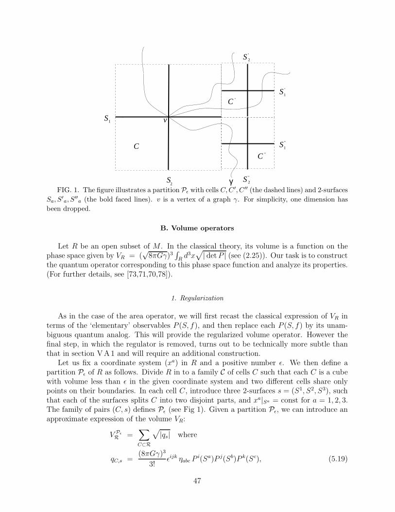
1

2S

vS

"

γ

C

CC

S

S

1

1

2

2S

S

’

’

’

"

"

FIG. 1. The figure illustrates a partition Pǫ with cells C,C ′, C ′′ (the dashed lines) and 2-surfaces

Sa, S′a, S

′′a (the bold faced lines). v is a vertex of a graph γ. For simplicity, one dimension has

been dropped.

B. Volume operators

Let R be an open subset of M . In the classical theory, its volume is a function on thephase space given by VR = (

√8πGγ)3

∫Rd3x√

| detP | (see (2.25)). Our task is to constructthe quantum operator corresponding to this phase space function and analyze its properties.(For further details, see [73,71,70,78]).

1. Regularization

As in the case of the area operator, we will first recast the classical expression of VR interms of the ‘elementary’ observables P (S, f), and then replace each P (S, f) by its unam-biguous quantum analog. This will provide the regularized volume operator. However thefinal step, in which the regulator is removed, turns out to be technically more subtle thanthat in section VA1 and will require an additional construction.

Let us fix a coordinate system (xa) in R and a positive number ǫ. We then define apartition Pǫ of R as follows. Divide R in to a family C of cells C such that each C is a cubewith volume less than ǫ in the given coordinate system and two different cells share onlypoints on their boundaries. In each cell C, introduce three 2-surfaces s = (S1, S2, S3), suchthat each of the surfaces splits C into two disjoint parts, and xa|Sa = const for a = 1, 2, 3.The family of pairs (C, s) defines Pǫ (see Fig 1). Given a partition Pǫ, we can introduce anapproximate expression of the volume VR:

V Pǫ

R =∑

C⊂R

√|qs| where

qC,s =(8πGγ)3

3!ǫijk ηabc P

i(Sa)P j(Sb)P k(Sc), (5.19)

47

It is easy to verify thatlimǫ→0

V Pǫ

R = VR ;

the dependence on the coordinate system and the partition disappears in the limit.To pass to the quantum theory, we need to define a consistent family of volume operators

VR,α, one for each graph α. Let us then fix a graph α and consider a partition Pǫ such thateach vertex v of α is the intersection point of the triplet of 2-surfaces S1, S2, S2 in somecell CV . Then, we can easily promote the approximate volume function V Pǫ

R to a quantum

operator V Pǫ

R,α:

V Pǫ

R,α =∑

C⊂R

√|qs,C |, where

qs =(8πGγ)3

3!ǫijk ηabc P

i(Sa)P j(Sb)P k(Sc), (5.20)

This operator is well-defined on Cyl(3)α , the space of thrice differentiable functions on Aα.

Furthermore, the limit ǫ→ 0, of the operator exists. However, unlike in the classical theory,it carries a memory of the partition Pǫ used in the regularization process. This is a newcomplication which did not occur in the case of the simpler area operators. But one canhandle it simply by averaging with respect to the essential background structures, used inthe construction of the partition Pǫ, prior to the removal of the regulator. This extra stepcan be carried out in detail [73]. The resulting operator is given by:

VR,α = κo

∑

v

√|qv,α|, where

qv,α = (8πγℓ2Pl)3 1

48

∑

e,e′,e′′

ǫijk ǫ(e, e′, e′′) J

(v,e)i J

(v,e′)j J

(v,e′′)k (5.21)

Here κo is an undetermined overall constant resulting from the averaging (usually set equalto 1); v runs over the set of vertices of α; each of e, e′, and e′′, over the set of edges of αmeeting at v; and ǫ(e, e′, e′′) is the orientation factor. (Thus, ǫ(e, e′, e′′) = 0 if the tangentvectors to the three edges are planar, i.e., lie in a 2-plane, at v, and ±1 if the orientationthey define is the same as or opposite to the fiducial orientation of M .) It is straightforwardto verify that this family of operators is consistent and hence defines a single densely definedoperator VR on H with domain Cyl(3).

Again, it is also meaningful to introduce in each Cyl(3)α a volume element operator

√q(x)α = κo

∑

v

δ(3)(x, v)√|qv, α|. (5.22)

The family of these operators is consistent and we thus have a densely defined operator√q(x) on H satisfying: VR =

∫Rd3x

√q(x).

Finally, in the classical the Poisson bracket Aia(x), VR between the connection at a

point x and the volume of a region containing that point is proportional to the co-triadei

a(x). This fact has been exploited to introduce co-triad operators which, in turn, haveled to a definition of the length operator [79] and features prominently in the discussion ofquantum dynamics of VIC [95–98].

48

2. Properties of volume operators

By inspection, VR is gauge invariant and covariant with respect to diffeomorphisms of M :under ϕ : M → M , we have VR → Vϕ·R. The total volume operator VM is diffeomorphisminvariant. Hence, its action is well-defined on the diffeomorphism invariant sub-space ofCyl⋆. This property plays an important role in the analysis of the Hamiltonian constraint.

Because of the presence of ǫ(e, e′, e′′) in (5.21), it is clear that qv,α = 0 if all edges meetingat v are planar. In particular, then, qv,α = 0 if v is a bi-valent vertex. More surprisingly,qv,α Ψ = 0 also for every tri-valent vertex v provided the state Ψ is invariant with respect tothe gauge transformations at v [68]. Indeed, let e, e′, e′′ be the edges of α which meet at v,and, for definiteness, suppose that ǫ(e, e′, e′′) = 1. Then, using gauge invariance at v, i.e.,

J(v,e)i + J

(v,e′)i + J

(v,e′′)i = 0, we obtain:

48

(8πγℓ2Pl)3qv,α Ψ = ǫijk J

(v,e)i J

(v,e′)j J

(v,e′′)k Ψ

= −ǫijkJ (v,e)i (J

(v,e)j + J

(v,e′′)j )J

(v,e′′)k Ψ

= −2i(J(v,e)j J

(v,e′′)k ηjk − J

(v,e)i J

(v,e′′)j ηij) Ψ

= 0. (5.23)

As with the area operator, it is easy to show that all eigenvalues of qv,α, VR,α and

VR are real and discrete. The spectrum —i.e., the set of all eigenvalues— of VR is thesame irrespective of the specific open region R. Given a point x ∈ M , the spectrum –i.e.,

the complete set of eigenvalues— of√q(x) is simply given by the union of the spectra

of the restrictions of qx to each of the (finite dimensional) spin-network spaces Sα,j,l in theorthogonal decomposition of H. Because of this property, many eigenvalues and eigenvectorsof the volume operators VR operators have been calculated in a number of special cases[70,74,76,77]. However the complete spectrum, or even an estimate of how the number ofeigenvalues grows for large volumes, is not yet known.

On the space of gauge invariant states, the simplest eigenvectors arise from 4-valentvertices. Even in this case, the full set of eigenvalues is not known. However, a technicalsimplification enables one to calculate the matrix element of the volume operator, whichhave been useful in the analysis of the quantum Hamiltonian constraint. Let v be a 4-valentvertex of α at which edges e, e′, e′′, e′′′ meet and consider the action of qv,α on the subspaceSα,j,l with lv = 0. Then,

qv,α = (8πγℓ2Pl)3 1

8κ(e, e′, e′′, e′′′) ǫijkJ

(v,e)i J

(v,e′)j J

(v,e′′)k (5.24)

where κ(e, e′, e′′, e′′′) ∈ −2,−1, 0, 2, 3, 4 depending on the diffeomorphism class of the fourtangent vectors at v. Using gauge invariance at v, the expression can be cast in the form:

qv,α = (8πγℓ2Pl)3 1

32iκ(e, e′, e′′, e′′′) [(J (v,e′) + J (v,e′′))2, (J (v,e) + J (v,e′′))2], (5.25)

which simplifies the task of calculating its matrix elements in the subspace Hα,j,l [78].

49

Finally, we note a property of the volume operator which plays an important role inquantum dynamics. Let R(x, ǫ) be a family of neighborhoods of a point x ∈ M . Then,

given any element Ψ of Cyl(3)α ,

limǫ→0

VR(x,ǫ) Ψ

exists but is not necessarily zero. This is a reflection of the ‘distributional’ nature of quantumgeometry.

3. ‘External’ regularization

Since the basic momentum variables are smeared on 2-surfaces, in the regularization pro-cedure for defining geometric operators one invariably begins by re-expressing the geometricfunctions on the classical phase space in terms of P (S, f). However, there is considerablefreedom in achieving this and, while different expressions may yield the same function onthe classical phase space when the regulator is removed, their quantum analogs need notshare this property. This is the standard ‘factor ordering problem’ of quantum theory. Inparticular, in the procedure summarized in section VB1, we expressed the volume of eachelementary cell C in terms of three 2-surfaces Sa (a = 1, 2, 3) which lie inside that cell. Thisstrategy goes under the name ‘internal regularization’. A natural alternative is to use the six2-surfaces Sα, α = 1, . . . 6 which bound the cell. This ‘external regularization’ strategy wasfirst introduced by Rovelli and Smolin [65] for gauge invariant states on tri-valent graphs.Although it was later realized that this volume operator is identically zero on these states[68], Rovelli and de Pietri [70] showed that the method extends also to non-trivial situations.

A detailed analysis [73] shows that this strategy is equally viable, once due attentionis paid to the convergence issues (that arise while removing the regulator) by carefullyconstructing the partition of R. Then, the final volume operator is again of the form (5.21)but given by:

V ExtR,α = κo

∑

v

√|qExt

v,α |, where

qExtv,α = (8πγℓ2Pl)

3 1

48

∑

e 6=e′ 6=e′′ 6=e

ǫijk J(v,e)i J

(v,e′)j J

(v,e′′)k (5.26)

A state Φ which is cylindrical with respect to a graph α and gauge invariant at a tri-valent vertex v is again annihilated by the new qExt

v,α . Furthermore, at gauge invariant 4-valent vertices, qExt

v,α agrees with qv,α, modulo a multiplicative factor which depends on thediffeomorphism class of the tangent vectors at v. In spite of this close relation on simplestates, the two operators are fundamentally different because of the absence of the orientationfactor ǫ(e, e′, e′′) in (5.26). In particular, because of this factor, the operators constructed insection VB1 know about the differential structure at vertices of graphs. By contrast, theaction of (5.26) is ‘topological’.

In the literature, internally regulated operators of section VB1 are used more often.For example, Thiemann’s analysis of properties volume operators in the continuum [78] andLoll’s analysis on lattices [74,75] refer to (5.21). The same is true of the volume operatorsused by Thiemann and others in the discussion of the Hamiltonian constraint.

50

VI. QUANTUM DYNAMICS

The quantum geometry framework provides the appropriate arena for a precise formu-lation of quantum Einstein’s equations. As indicated in section II, because of the difficultproblems of background independent regularization of products of operator valued distribu-tions, quantum Einstein’s equations still remain formal in geometrodynamics. In connection-dynamics, by contrast, we have a well-defined Hilbert space H of kinematical states and itis natural to attempt to represent left sides of quantum Einstein’s equations by well-definedoperators on H. Now, in interacting (low dimensional) quantum field theories, there isa delicate relation between quantum kinematics and dynamics: unless the representationof the basic operator algebra is chosen appropriately, typically, the Hamiltonian fails tobe well-defined on the Hilbert space. For a complicated system such as general relativity,then, one would imagine that the problem of choosing the ‘correct’ kinematic representationwould be extremely difficult (see, e.g. [85]). However, a major simplification arises from thestriking uniqueness result discussed at the end of section IV: the requirement of generalcovariance picks out a unique representation of the algebra generated by holonomies andelectric fluxes [55–58]. Therefore we have a single arena for background independent theo-ries of connections and a natural strategy for implementing dynamics provided, of course,this mathematically natural, kinematical algebra is also ‘physically correct’. (This provisoexists also for the quantum field theories referred to above.) As we will summarize in thissection, this strategy has led to well-defined candidates for quantum Einstein’s equations.

Recall from section II that because general relativity has no background fields, the theoryis fully constrained in its phase space formulation. To pass to the quantum theory, one canuse one of the two standard approaches: i) find the reduced phase space of the theoryrepresenting ‘true degrees of freedom’ thereby eliminating the constraints classically andthen construct a quantum version of the resulting unconstrained theory; or ii) first constructquantum kinematics for the full phase space ignoring the constraints, then find quantumoperators corresponding to constraints and finally solve quantum constraints to obtain thephysical states. Loop quantum gravity follows the second avenue, which was initiated byDirac.25 This program has been carried out to completion in many simpler systems, suchas 2+1 dimensional gravity [35,2,5] and a number of mini-superspaces in 3+1 dimensions[86], where one can explicitly see that the procedure incorporates all of quantum Einsteinequations. Readers who are not familiar with quantization of constrained systems shouldfirst familiarize themselves with the subject through simple examples (see, e.g. [87]). Toadequately handle conceptual and technical intricacies encountered in general relativity,

25Thus, in the canonical approach, the entire quantum dynamics is fully incorporated by solving

quantum constraints. This may seem surprising because in the classical theory we have both the

constraint and the evolution equations. However, because the evolution is generated by constraints

in the Hamiltonian framework, in the quantum theory dynamics is encoded in the operator con-

straints. A simple example is provided by a free particle in Minkowski space, where the constraint

gabpapb + m2 = 0 on the classical phase space becomes 2φ − m2φ = 0, governing dynamics in the

quantum theory

51

Dirac’s original program has to be modified and extended suitably. We will use the resultingframework, called refined algebraic quantization. For further details, see, e.g., [88,89,141].

A. The Gauss constraint

Recall from section II that the Gauss constraint, Gi ≡ DaPai = 0, generates internal

SU(2) rotations on the phase space of general relativity. More precisely, given an su(2)-valued function ξ on M , we can use it as a smearing field to obtain a phase space function

CG(ξ) = −∫

M

d3xP ai (x)Daξ

i(x) , (6.1)

which generates infinitesimal canonical transformations (A,P ) → (A−Dξ, P+[ξ, P ]). Usingthe heuristic ansatz P → −i~δ/δA, it is straightforward to promote CG(ξ) to a well-defined

operator on H [89]. For any Ψα ∈ Cyl(1)α we have:

CG(ξ) Ψα = ~∑

v

∑

e

(ξi(v)J(v,e)i ) Ψα (6.2)

where the first sum extends over all vertices v of α and the second over all edges e meetingat v. Apart from the factor of ~, this action coincides with that of the generator of gaugetransformations on Hα discussed in section IVB2. This family of operators on Hα is con-sistent and defines a self-adjoint operator on H which we will also denote by CG(ξ). Finitegauge transformations are generated by the 1-parameter unitary groups generated by theseoperators.

Physical states belong to the kernel HGinv of CG(ξ) for all ξ ∈ su(2). Because the action

of CG is familiar, the kernel is easy to find: In terms of the Hilbert space decompositionsdiscussed in section IVC3,

HGinv =

⊕

α,j

H′α,j,l=0 .

Note that these states are automatically invariant under generalized gauge transformationsin G and can be regarded as functions on the reduced quantum configuration space A/G.HG

inv is a sub-space of H because zero is in the discrete part of the spectrum of the constraintoperator CG(ξ). In particular, HG

inv inherits a Hilbert space structure from H and HGinv =

L2(A/G, dµGo ), where dµG

o is the natural measure on A/G, the push-forward of dµo underthe natural projection map from A to A/G. Every gauge invariant operator —such as areasAS and volumes VR of section V— has a well defined action on HG

inv.The fact that the Gauss constraint could be imposed so easily and that the structure of

HGinv is so simple hides the non-triviality of the procedure. For example if, in place of A,

one uses one of the standard distribution spaces as the quantum configuration space, theimposition of the Gauss constraint and construction of the Hilbert space of physical statesbecomes complicated and it is not obvious that these difficulties can be surmounted.

52

B. The diffeomorphism constraint

Let us now consider the diffeomorphism constraint. We will find that the imposition ofthis constraint is more complicated because of a key difference: While there is an infinitedimensional subspace HG

inv of H that is invariant under the SU(2) gauge rotations, sincediffeomorphisms move graphs, the only element of H left invariant by the action of alldiffeomorphisms is the constant function on A ! As a result, solutions to the quantumconstraints lie not in the kinematical Hilbert space H but in a larger space, the dual Cyl⋆ ofCyl. This is not unusual. Even in simple quantum mechanical systems, such as a particlein R3 with a constraint px = 0, solutions to the constraint fail to have finite norm in thekinematic Hilbert space L2(R3) and belong to a larger space, e.g., the space of distributionsin R3. In a similar fashion, we will be able to construct a systematic framework and obtainthe general solutions to the diffeomorphism constraint.

1. Strategy

Recall from section IIC 3 that each vector field Na on M defines a constraint functionCDiff( ~N) on the gravitational phase space:

CDiff( ~N) =

∫

M

d3x(NaF i

abPbi − P aDa(N

bAib)). (6.3)

Under infinitesimal canonical transformations generated by CDiff( ~N), we have: (A,P ) 7→(A+L ~NA, P +L ~NP ). In the mathematically precise literature on constrained systems it isthe finite gauge transformations generated by constraints that are of primary interest in thequantum theory. Therefore, in our case, it is appropriate to impose the diffeomorphism con-straint by demanding that the physical states be left invariant under finite diffeomorphismsϕ generated by ~N . Since the measure dµo on A is diffeomorphism invariant, the inducedaction of ϕ on H is unitary. Thus, given the vector field Na, we obtain a 1-parameter familyϕ(λ) of diffeomorphisms on M and a corresponding family ϕ(λ) of unitary operators on H.But this family fails to be weakly continuous in λ because Cylα is orthogonal to Cylϕ·α if ϕmoves α. Hence, the infinitesimal generator of ϕ(λ) fails to exist. (For details, see AppendixC in [89].) However, this creates no obstacle because, for the quantum implementation ofthe constraint, we can work directly with finite diffeomorphisms: Physical states are to beinvariant under the induced action ϕ of appropriate diffeomorphisms ϕ on M .

To solve the constraint, we will use the ‘group averaging procedure’, generally avail-able for such constraints26 (see, e.g., [88,89]): Physical states will be obtained by averag-ing elements of Cyl with respect to the induced action of the diffeomorphism group. It

26The quantum Gauss constraint can be rigorously implemented also through group averaging

over G. The final result is the same as that obtained in sectionVI A. For pedagogical purposes, in

section VI A we adopted a procedure which is closer to the one followed for the scalar constraint

in section VI C.

53

is intuitively obvious that the result of group averaging will be diffeomorphism invariant.However, although one begins with states in Cyl, the result naturally belongs to Cyl⋆, the al-gebraic dual of Cyl.27 In finite dimensional constrained systems, one generally uses a triplet,S ⊂ L2(Rn) = Hkin ⊂ S⋆, where S is typically the space of smooth functions with rapid de-cay at infinity, and S⋆, the space of distributions. The solutions to constraints are obtainedby averaging elements of S with respect to the group generated by constraints and they typ-ically belong to S⋆ rather than to the kinematical Hilbert space Hkin [88,141]. In the presentcase, we have a completely analogous situation and now the triplet is Cyl ⊂ H ⊂ Cyl⋆.

Finally there is an important technical subtlety coming from the fact that, graphs α arerequired to have closed-piecewise analytic edges. The classical phase space, on the otherhand, consists of smooth (i.e. Cn) fields (A,P ). Smooth diffeomorphisms ϕ correspond tofinite canonical transformations generated by the constraint (6.3) and have a well-definedaction on the phase space. It is just that the action does not extend to our full algebraof ‘elementary variables’ since their definition involves closed-piecewise analytic edges andsurfaces. A natural strategy to impose the diffeomorphism constraint, therefore, is to enlargethe framework and allow smooth edges and surfaces. This is possible [47,63,92,64] but thenthe technical discussion becomes much more complicated because, e.g., two smooth curvescan intersect one another at an infinite number of points. Here we will adopt an ‘in-between’approach and use the sub-group Diff of all Cn diffeomorphisms of M , introduced in sectionIVC5, which has a well-defined action on our elementary variables and the Hilbert spaceH. From a physical perspective, this is more appropriate than averaging with respect tojust the analytical diffeomorphisms and from a mathematical perspective it enables us tobypass the complications associated with non-analytical edges and surfaces.

2. Physical states

Our task now is to construct the general solution to the diffeomorphism constraint. Forthis, we will use the spin-network decomposition (4.46): H = ⊕α H′

α. Let us begin byintroducing some notation. Given a graph α, denote by Diffα the sub-group of Diff whichmaps α to itself and by TDiffα its subgroup which has trivial action on α, i.e., which preserves

every edge of α and its orientation. The induced action, TDiffα, is trivial on Cylα. Next,let Diffα be the group of all the diffeomorphisms that preserve α. Then, the quotient

GSα = Diffα/TDiffα, (6.4)

is the group of graph symmetries of α. It is a finite group and it has a non-trivial inducedaction GSα on Cylα. In the group averaging procedure, consistency requires that one mustdivide by the ‘volume’ of the orbits of these groups [89].

27In the end, one would have to introduce a suitable topology on Cyl which is finer than the

Hilbert space topology and let Cyl⋆ be the topological dual of Cyl. The program is yet to reach

this degree of sophistication and, for the moment, the much bigger algebraic dual is used.

54

To construct the general solution to the diffeomorphism constraint, we proceed in twosteps. First, given any Ψα ∈ H′

α, we average it using only the group of graph symmetries

and obtain a projection map Pdiff,α from H′α to its subspace which is invariant under GSα:

Pdiff,αΨα :=1

Nα

∑

ϕ∈GSα

ϕ ⋆Ψα, (6.5)

where Nα is the number of the elements of GSα (the volume of the obit of GS) and ϕ ⋆ Ψa

denotes the pull-back of Ψα under ϕ. The map extends naturally to a projection Pdiff fromH = L2(A, dµo) to its subspace which is invariant under GSα for all α.

In the second step, we wish to average with respect to the remaining diffeomorphismswhich move the graph α. This is a very large group and the result of averaging now belongsto Cyl⋆ rather than H. Thus, to each Ψα ∈ H′

α, we now associate an element (η(Ψα)| ∈ Cyl⋆,defined by its (linear) action on arbitrary cylindrical functions |Φβ〉 ∈ Cyl:

(η(Ψα) |Φβ〉 =∑

ϕ∈Diff/Diffα

〈ϕ ⋆ Pdiff,αΨα, Φβ〉, (6.6)

where the bracket on the right side denotes the inner product between elements of H.Although ϕ ∈ Diff/Diffα contains an infinite number of elements ϕ, for any given β onlya finite number of terms are non-zero, whence η(Ψα) is well-defined. However, there is novector η in H such that 〈η, Φβ〉 equals the right side of (6.6) for all Φβ ∈ Cyl. Thus, (η(Ψα)|is a ‘genuine distribution’ on A rather than a function. Because of the diffeomorphisminvariance of the scalar product on H, η(Ψα) is invariant under the action of Diff(M):

(η(Ψα) |ϕ ⋆ Φβ〉 = (η(Ψα) |Φβ〉 (6.7)

for all ϕ ∈ Diff(M). We will denote the space of these solutions to the diffeomorphismconstraint by Cyl⋆diff . Finally, since Ψα was an arbitrary element of Cyl, we have constructeda map:

η : Cyl → Cyl⋆diff . (6.8)

Thus, every element of Cyl gives rise, upon group averaging, to a solution to the diffeomor-phism constraint. In this sense, we have obtained the general solution to the diffeomorphismconstraint. The map η is the analog of the projection from H to its gauge invariant sub-space HG

inv in the case of the Gauss constraint. However, because of the differences betweenthe two constraints discussed above, η is not a projection since it maps Cyl onto a differentspace Cyl⋆diff . Nonetheless, the group averaging procedure naturally endows the solutionspace with a Hermitian inner product,

(η(Ψ) | η(Φ)) := (η(Ψ) |Φ〉 , (6.9)

since one can show that the right side is independent of the specific choice of Ψ and Φ madein the averaging [88,89]. (For subtleties, see [89,141]). We will denote by Hdiff the Cauchycompletion of Cyl⋆diff . Finally, we can obtain the general solution to both the Gauss and the

55

diffeomorphism constraints by simply restricting the initial Ψ ∈ Cyl to be gauge invariant,i.e., to belong to Cyl ∩HG

inv. We will denote this space of solutions by Cyl⋆inv:

Cyl⋆inv = η(Cyl ∩HGinv) (6.10)

What is the situation with respect to operators? Note first that there do exist non-trivial(gauge and) diffeomorphism invariant operators on Cyl; an example is the total volumeoperator VM . Let O be such an operator. Its dual, O⋆, is well defined in Cyl⋆inv:

(O⋆η(Ψ) |Φ〉 := (η(Ψ) | OΦ〉 . (6.11)

(Furthermore, one can show that O⋆ preserves the image of H′α for very α.) The operator O⋆

is self adjoint with respect to the natural scalar product (6.9) on Hdiff if and only if O is selfadjoint in H. This property shows that the scalar product on H is not only mathematicallynatural but also ‘physically correct’.

Let us summarize. The basic idea of the procedure used to solve the diffeomorphismconstraint is rather simple: One averages the kinematical states with the action of thediffeomorphism group to obtain physical states. But the fact that this procedure can beimplemented in detail is quite non-trivial. For example, a mathematically precise imple-mentation still eludes the geometrodynamics program. Furthermore, even the final answercontains certain subtleties. We will conclude by pointing them out.

Remarks: i) Note that while (η(Ψ)| is a solution to the diffeomorphism constraint forany Ψ ∈ Cyl, it is not true that there is a 1-1 correspondence between elements of Cyl andsolutions to the diffeomorphism constraint. This is because the map η has a non-trivialkernel. In particular, the projection map Pdiff itself has a non-trivial kernel which, by (6.6)is also in the kernel of η. (In addition, elements of Cyl of the form a0Ψα + a1ϕ1 ⋆Ψα + ...+anϕn ⋆Ψα, with a0 + ...+ an = 0 are also in the kernel of η.) Therefore statements suchas “solutions to the diffeomorphism constraint are diffeomorphism classes of spin networkstates” that one often finds in the literature are only heuristic.ii) One also finds claims to the effect that the diffeomorphism constraint can be imposedsimply by replacing spin networks embedded in a manifold M by abstract, non-embeddedspin networks. Within the systematic approach summarized in this section, these claims aresimply incorrect (for a detailed discussion in the context of 2+1 gravity on a lattice, see,e.g., [93]). In particular a graph, one of whose edges is knotted, can not be mapped by adiffeomorphism to one in which all edges are unknotted, whence the mapping η sends spin-network states associated with the two graphs to distinct solutions to the diffeomorphismconstraint. As abstract, non-embedded graphs, on the other hand, they can be equivalentand define the same spin-network functions. One can imagine a new approach in whichone simply declares that the diffeomorphism constraint is to be incorporated by replacingembedded spin-networks by abstract ones. But since the original diffeomorphism constraintacts on the basic canonical variables (A,E) on M and the action can be transferred tographs only if they are embedded, it would be difficult to justify such an approach from firstprinciples.iii) Note that there are continuous families of 4 or higher valent graphs which can not bemapped to one another by Cn diffeomorphisms with n > 0. Consequently, states in Hdiff

based on two of these graphs are mutually orthogonal. Thus, even though we have ‘factored

56

out’ by a very large group Diff, the Hilbert space Hdiff is still non-separable. However, ifwe were to let n = 0, i.e. consider homeomorphisms of M which preserve the family ofgraphs under consideration, then these ‘problematic’ continuous families of graphs wouldall be identified in the group averaging procedure and the Hilbert space of solutions to thediffeomorphism constraint would be separable. However, since the classical constraints donot generate homeomorphims, and furthermore homeomorphisms do not even have a well-defined action on the phase space, it is difficult to ‘justify’ this enlargement of Diff fromdirect physical considerations.iv) Note that Cyl⋆diff is a proper subset of the space Cyl⋆Diff of all elements of Cyl⋆ invariantunder Diff. However, every (Ψ| ∈ Cyl⋆Diff can be uniquely decomposed as

(Ψ| =∑

[α]

(Ψ[α]| , with (Ψ[α]| ∈ η(Cylα), (6.12)

where [α] runs through the diffeomorphism classes of graphs. The sum on the right side isuncountable but the result is a well-defined element of Cyl⋆ because, in its action on anycylindrical function, only finite number of the terms fail to vanish.

C. The Scalar Constraint

The canonical transformations generated by the Gauss and the diffeomorphism con-straints are kinematical gauge symmetries of the classical theory in the sense that, in thespace-time picture, they operate at a ‘fixed time’. The crux of quantum dynamics lies inthe scalar constraint. One can imagine implementing it in the quantum theory also by agroup averaging procedure. However, this strategy is difficult to adopt because the finitecanonical transformations generated by this constraint are not well-understood even at theclassical level. Therefore, one follows the procedure used for the Gauss constraint: constructa quantum operator corresponding to the classical, smeared constraint function and thenseek its kernel. Because the form of this constraint is so intricate, its implementation isstill rather far from being as clean and complete as that of the other two constraints. Inparticular, genuine ambiguities exist in the regularization procedure and distinct avenueshave been pursued [95-102]. What is non-trivial at this stage is the existence of well-definedstrategies. Whether any of them is fully viable from a physical perspective is still an openissue. In this summary, we will essentially follow the most developed of these approaches,introduced by Thiemann [95–97]. However, to bring out quantization ambiguities we havegeneralized the method, emphasizing points at which there is freedom to modify the originalprocedure and still arrive at a well-defined constraint operator. Our emphasis is more onclarifying the underlying conceptual structure than on providing efficient calculational tools.

1. Regulated classical expression

As with area and volume operators, our first task is to re-express the classical expres-sion of the scalar constraint as a Riemann sum involving only those phase space functionswhich have direct quantum analogs. Recall from section II that in terms of real connection

57

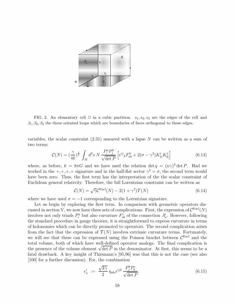
FIG. 2. An elementary cell 2 in a cubic partition. s1, s2, s3 are the edges of the cell and

β1, β2, β3 the three oriented loops which are boundaries of faces orthogonal to these edges.

variables, the scalar constraint (2.31) smeared with a lapse N can be written as a sum oftwo terms:

C(N) = (γ

4k)

12

∫

M

d3xNP a

i Pbj√

detP

[ǫijkF

kab + 2(σ − γ2)Ki

[aKjb]

](6.13)

where, as before, k = 8πG and we have used the relation det q = (κγ)3 detP . Had weworked in the +,+,+,+ signature and in the half-flat sector γ2 = σ, the second term wouldhave been zero. Thus, the first term has the interpretation of the the scalar constraint ofEuclidean general relativity. Therefore, the full Lorentzian constraint can be written as

C(N) =√γCEucl(N) − 2(1 + γ2)T (N) (6.14)

where we have used σ = −1 corresponding to the Lorentzian signature.Let us begin by exploring the first term. In comparison with geometric operators dis-

cussed in section V, we now have three sets of complications. First, the expression of CEucl(N)involves not only triads P a

i but also curvature F iab of the connection Ai

a. However, followingthe standard procedure in gauge theories, it is straightforward to express curvature in termsof holonomies which can be directly promoted to operators. The second complication arisesfrom the fact that the expression of T (N) involves extrinsic curvature terms. Fortunately,we will see that these can be expressed using the Poisson bracket between CEucl and thetotal volume, both of which have well-defined operator analogs. The final complication isthe presence of the volume element

√detP in the denominator. At first, this seems to be a

fatal drawback. A key insight of Thiemann’s [95,96] was that this is not the case (see also[100] for a further discussion). For, the combination

eia :=

√kγ

2ηabcǫ

ijkP b

j Pck√

detP. (6.15)

58

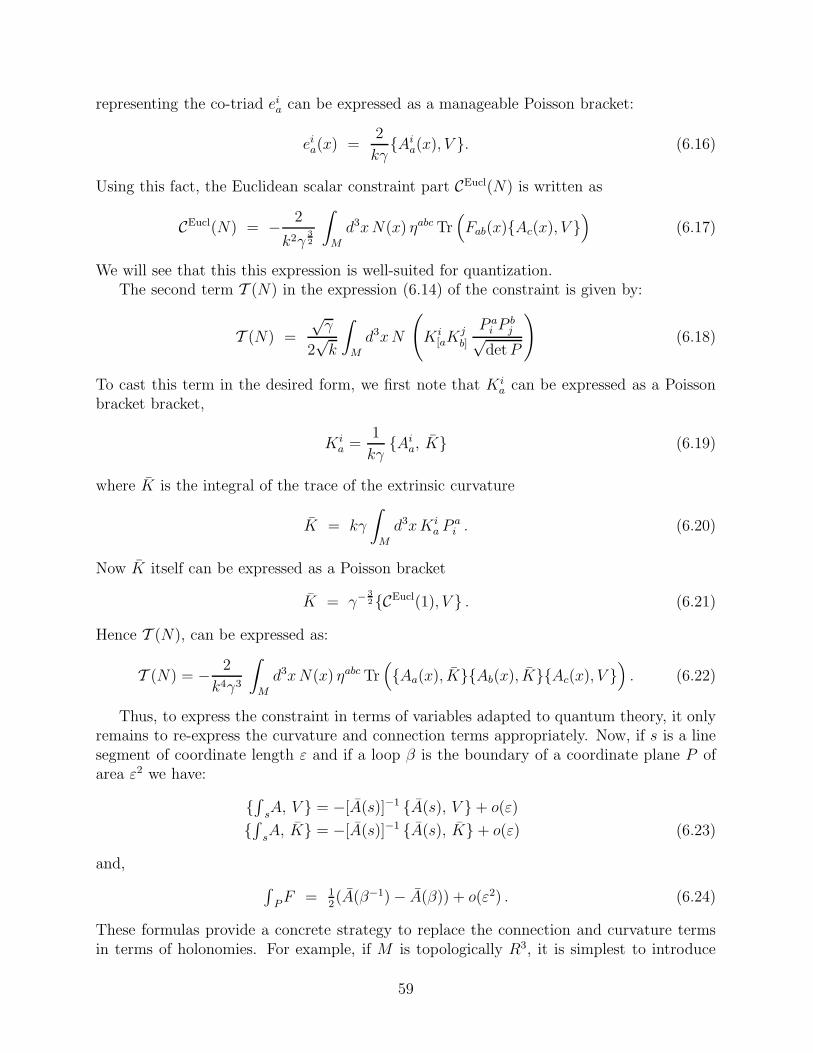
representing the co-triad eia can be expressed as a manageable Poisson bracket:

eia(x) =

2

kγAi

a(x), V . (6.16)

Using this fact, the Euclidean scalar constraint part CEucl(N) is written as

CEucl(N) = − 2

k2γ32

∫

M

d3xN(x) ηabc Tr(Fab(x)Ac(x), V

)(6.17)

We will see that this this expression is well-suited for quantization.The second term T (N) in the expression (6.14) of the constraint is given by:

T (N) =

√γ

2√k

∫

M

d3xN

(Ki

[aKjb]

P ai P

bj√

detP

)(6.18)

To cast this term in the desired form, we first note that Kia can be expressed as a Poisson

bracket bracket,

Kia =

1

kγAi

a, K (6.19)

where K is the integral of the trace of the extrinsic curvature

K = kγ

∫

M

d3xKia P

ai . (6.20)

Now K itself can be expressed as a Poisson bracket

K = γ−32CEucl(1), V . (6.21)

Hence T (N), can be expressed as:

T (N) = − 2

k4γ3

∫

M

d3xN(x) ηabc Tr(Aa(x), KAb(x), KAc(x), V

). (6.22)

Thus, to express the constraint in terms of variables adapted to quantum theory, it onlyremains to re-express the curvature and connection terms appropriately. Now, if s is a linesegment of coordinate length ε and if a loop β is the boundary of a coordinate plane P ofarea ε2 we have:

∫

sA, V = −[A(s)]−1 A(s), V + o(ε)

∫

sA, K = −[A(s)]−1 A(s), K + o(ε) (6.23)

and,

∫PF = 1

2(A(β−1) − A(β)) + o(ε2) . (6.24)

These formulas provide a concrete strategy to replace the connection and curvature termsin terms of holonomies. For example, if M is topologically R3, it is simplest to introduce

59

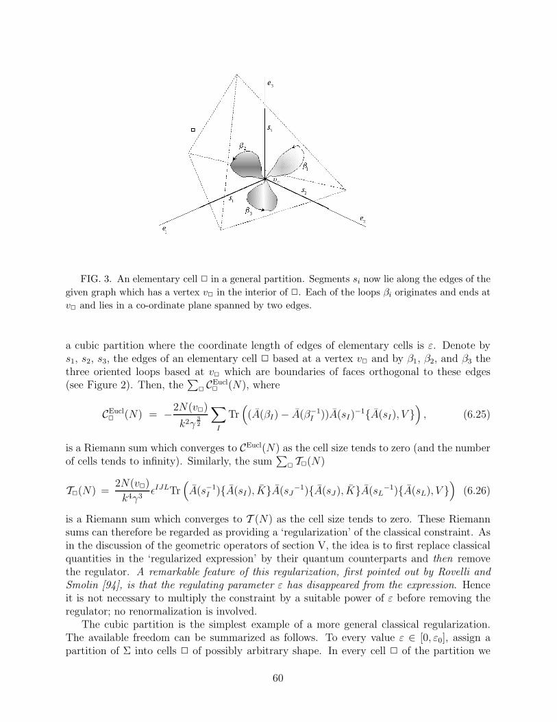
FIG. 3. An elementary cell 2 in a general partition. Segments si now lie along the edges of the

given graph which has a vertex v2 in the interior of 2. Each of the loops βi originates and ends at

v2 and lies in a co-ordinate plane spanned by two edges.

a cubic partition where the coordinate length of edges of elementary cells is ε. Denote bys1, s2, s3, the edges of an elementary cell 2 based at a vertex v2 and by β1, β2, and β3 thethree oriented loops based at v2 which are boundaries of faces orthogonal to these edges(see Figure 2). Then, the

∑2CEucl

2(N), where

CEucl2

(N) = −2N(v2)

k2γ32

∑

I

Tr((A(βI) − A(β−1

I ))A(sI)−1A(sI), V

), (6.25)

is a Riemann sum which converges to CEucl(N) as the cell size tends to zero (and the numberof cells tends to infinity). Similarly, the sum

∑2T2(N)

T2(N) =2N(v2)

k4γ3ǫIJLTr

(A(s−1

I )A(sI), KA(sJ−1)A(sJ), KA(sL

−1)A(sL), V )

(6.26)

is a Riemann sum which converges to T (N) as the cell size tends to zero. These Riemannsums can therefore be regarded as providing a ‘regularization’ of the classical constraint. Asin the discussion of the geometric operators of section V, the idea is to first replace classicalquantities in the ‘regularized expression’ by their quantum counterparts and then removethe regulator. A remarkable feature of this regularization, first pointed out by Rovelli andSmolin [94], is that the regulating parameter ε has disappeared from the expression. Henceit is not necessary to multiply the constraint by a suitable power of ε before removing theregulator; no renormalization is involved.

The cubic partition is the simplest example of a more general classical regularization.The available freedom can be summarized as follows. To every value ε ∈ [0, ε0], assign apartition of Σ into cells 2 of possibly arbitrary shape. In every cell 2 of the partition we

60

define edges sJ , J = 1, ..., ns and loops βi, i = 1, ..., nβ, where ns, nβ may be different fordifferent cells (see Figure 3). Finally, fix an arbitrarily chosen representation ρ of SU(2).This entire structure will be denoted by Rε and called a permissible classical regulator if thefollowing property holds:

limε→0

CEuclRε

(A,E) = CEucl(A,E) and limε→0

TRε(A,E) = T (A,E) , (6.27)

where

CEuclRε

=∑

2

CEuclRε2

, (6.28)

CEuclRε

=N(v2)

k2γ32

∑

iJ

CiJTr( (ρ[A(βi)] − ρ[A(β−1

i )])ρ[A(sJ

−1)]ρ[A(sJ)], V ), (6.29)

TRε=∑

2

TRε2 (6.30)

TRε2 =N(v2)

k4γ3

∑

I,J,K

T IJKTr(ρ[A(s−1

I )]ρ[A(sI)], Kρ[A(sJ−1)]ρ[A(sJ)], K

× ρ[A(sK−1)]ρ[A(sK)], V

); (6.31)

and, CiJ , T IJK are fixed constants, independent of the scale parameter ε. A large family ofthe classical regulators can be constructed by modifications of the cubic example, changingthe shape of the cells, loops and edges, and their relative positions suitably.

2. The quantum scalar constraint

Our task is to first promote the regulated classical constraint to a quantum operator andthen remove the regulator. In the detailed implementation of this procedure, one encountersthree non-trivial issues.

As in the case of geometric operators, the first step is rather straightforward becausethe regulated expressions involve only those phase functions which have direct quantumanalogs. However, while the ‘obvious’ quantum operator would be well-defined on stateswhich are cylindrical with respect to any one graph, at the end we have to ensure that theresulting family of operators is consistent. This is the first non-trivial issue. The simplestway to address it is to use the decomposition H = ⊕αH′

α of the Hilbert space, introducedin Section IVC3, and define the quantum constraint on each H′

α separately. Because of theorthogonality of any two H′

α, the resulting family of operators would then be automaticallyconsistent.

Let us begin with CEuclRε

. Fix a subspace H′α of H. The quantum operator can be obtained

simply by promoting the holonomies and volume functions to operators and replacing thePoisson brackets by 1/i~-times commutators. Thus, for any given graph α and ε > 0,

CEuclRε,α

(N) :=∑

2

CE2

(N) (6.32)

61

with

CEucl2

(N) := −iN(v2)

k2γ32 ~

∑

iJ

CiJTr( (ρ[A(βi)] − ρ[A(β−1

i )])ρ[A(sJ

−1)][ρ[A(sJ)], V

]),

(6.33)

is a densely defined operator on H′α with domain Dα = H′

α ∩Cylα for any classical regulatorRε. We now encounter the second non-trivial issue: we have to ensure that the final operatoris diffeomorphism covariant. To address it, we need to use regulators which are not fixed buttransform covariantly as we move from a graph α to any of its images under diffeomorphisms.Therefore, we will restrict our regulators appropriately.

A diffeomorphism covariant quantum regulator Rε,α is a family of permissible classicalregulators, one for each choice of the graph α, satisfying the following properties:

a) the partition is sufficiently refined in the sense that every vertex v of α is contained inexactly one cell of Rε,α; and,

b) if (α, v) is diffeomorphic to (α′, v′) then, for every ε and ε′, the quintuple(α, v,2, (sI), (βJ)) is diffeomorphic to the quintuple (α′, v′,2′, (s′I), (β

′J)) where 2 and

2′ are the cells of Rε and R′

ε respectively, containing v and v′ respectively. 28

Such diffeomorphism compatible quantum regulators exist; an explicit example is given in[96]. Given such a Rε,α, for every value of ε, the operators CEucl

Rε,α(N) are densely defined

on H′α with a common domain Dα. This family of operators determines a densely defined

operator CEuclRε

on the full Hilbert space H with domain Cyl, independently of the value of

ε. Furthermore, for any value of ε, this domain is mapped to itself by the operator CEuclRε

.Thus, it only remains to remove the regulator. Here we encounter the third non-trivial

issue. Typically CEuclRε,α

|Ψα〉 is orthogonal to CEuclRε′,α

|Ψα〉 if ε 6= ε′, whence the operator does

not converge (even in the weak topology) on H. This is a rather general problem associatedwith the topology of H; we encountered it also while defining the operator analog of thediffeomorphism constraint CDiff( ~N). Recall, however, that solutions to the diffeomorphismconstraint also fail to lie in the kinematical Hilbert space H; they belong to Cyl⋆, thealgebraic dual of Cyl. Therefore, for the consistency of the whole picture, what we need isthe action of the scalar constraint only on a sufficiently large subspace of Cyl⋆ and not onH. And this action is well-defined and non-trivial. More precisely, for each (Ψ| ∈ Cyl⋆, theaction of the regulated constraint operator is naturally given by:

[(Ψ|CEucl

Rε

]|Φ〉 := (Ψ|

[CEucl

Rε|Φ〉]

(6.34)

for all |Φ〉 ∈ Cyl⋆. We can now remove the regulator in the obvious fashion. Define

28We need the restriction only on cells which contain vertices because the properties of the volume

operator imply that the action of CEucl2

is non-trivial only if one of the segments sI of the regulator

intersects a vertex of α.

62

CEucl(N) = limε→0

CEuclRε

(N) (6.35)

via[(Ψ|CEucl(N)

]|Φ〉 = lim

ε→0(Ψ|

[CEucl

Rε(N)|Φ〉

]. (6.36)

Note that the limit has to exist only pointwise, i.e., for each |Φ〉 ∈ Cyl separately. As aconsequence the domain of the operator, the set of (Ψ| in Cyl⋆ for which the limit exists,is quite large. In particular, as discussed below, it includes a large class of solutions to thediffeomorphism constraints. The term T (N) in the scalar constraint can be handled in a

completely parallel fashion. Specifically, we can first define the operator ˆK through

ˆK :=i

~γ32

[V , CE(1)] (6.37)

and use ˆK and the quantum regulator Rε,α to define the regulated operator T2(N):

(Ψ|T2(N) =iN(v2)

k4γ3~3T IJK (Ψ|Tr

(A(s−1

I )[AsI, ˆK]A(sJ

−1)[A(sJ), ˆK]

×A(sK−1)[A(sK), V ]

), (6.38)

on the domain Cyl⋆. Collecting these definitions, we now have a regulated scalar constraintoperator:

(Ψ| CRε(N) := (Ψ|

(√γCEucl

Rε(N) − 2(1 + γ2)

∑

2

T2(N))

(6.39)

for all (Ψ| ∈ Cyl⋆. Again, we can remove the regulator by taking the limit as ε → 0 as in(6.36). By construction, the action of this operator is diffeomorphism covariant. Thus, eachdiffeomorphism covariant quantum regulator defines a scalar constraint operator. Since thereis a great deal of freedom in choosing these regulators, there is considerable quantizationambiguity. Nonetheless, all these constructions exhibit some very non-trivial properties. Wewill conclude this section by providing two illustrations.

First, as mentioned in the beginning of this section, it is significant that well definedprescriptions exist to give precise meaning to quantum Einstein equations in a backgroundindependent setting. In geometrodynamics, for example, the Wheeler-DeWitt equation stillremains only formal. Secondly, these constructions match surprisingly well with the solutionsof the diffeomorphism constraint. To see this note first that, irrespective of the choice of thediffeomorphism covariant quantum regulator, up to diffeomorphisms, the operator CRε

(N)is independent of ε: for every ε, ε′ and |Ψ〉 ∈ Cyl, there is a diffeomorphism ϕ such that

CRε′(N) |Ψ〉 = UϕCRε′

(N)|Ψ〉 , (6.40)

for every N . Next, suppose that (Ψ| ∈ Cyl⋆ is diffeomorphism invariant. Then, for everylapse function N , the result (Ψ|(CRε

(N)), is in fact independent of ε, and so is the expressionunder the limit on the right hand side of (6.39). Hence the regulator can be removed trivially

63

[94]. Thus because of the form of the regulated operators, diffeomorphism invariant statesin Cyl⋆ (constructed by group averaging elements of H′

α ∩ Cylα) are automatically in thedomain of the scalar constraint operator. This tight matching between the way in which thetwo constraints are handled is quite non-trivial.

Remark: In the original construction by Thiemann [96], the Hamiltonian constraint op-erator was defined on Cyl⋆diff . Now, as we saw in section II, the Poisson bracket of any twoscalar constraints is given by a diffeomorphism constraint in the classical theory. Therefore,on diffeomorphism invariant states, one would expect the quantum scalar constraint opera-tors to commute. Irrespective of the choice of the regulator Rε, they do. To obtain a morestringent test, the domain of the Thiemann operator was extended slightly in [100,101]. Theextended domain, called the ‘habitat’ [101], also includes certain elements of Cyl⋆ whichare not diffeomorphism invariant. Nonetheless, it turned out that the commutator betweenscalar constraints continues to vanish on the habitat. This may seem alarming at first.However, it turns out that the quantum operator corresponding to the classical Poissonbracket also annihilates every state in the habitat [100]. Thus, there is no inconsistency;the habitat just turned out to be too small to provide a non-trivial viability criterion ofthis quantization procedure. The domain of the operator introduced in this section includesthe habitat and the same result continues to hold. More importantly, it is likely that thisdomain is significantly larger and may contain semi-classical states. If this turns out to bethe case, stronger viability criteria to test this quantization procedure will become available.In particular, in addition to the relation to the classical Poisson algebra of constraints, onemay be able to analyze the relation between the classical evolution and the action of theconstraint on semi-classical states.

3. Solutions to the scalar constraint

In this section, we will illustrate how the difficult problem of finding solutions to thequantum constraints can be systematically reduced to a series of simpler problems. For this,we will need to make the quantum regulator Rε,α more specific.

The most convenient class of regulators requires some modifications in the original con-struction due to Thiemann. Restrictions defining this class can be summarized as follows.Fix a graph α and consider a cell 2 containing a vertex v in the partition of M defined bythe regulator. The first restriction is that every edge sk assigned to 2 must be a propersegment of an edge incident at v, oriented to be outgoing at v. The next restriction is on theclosed loops β. To every pair of edges eI , eJ assign a triangular closed loop βIJ such that:i) the loop contains v but no other point in the graph α; ii) it lies ‘between’ the 2-edges, ina 2-plane containing the edges, where the plane is defined up to diffeomorphisms preservingα; and iii) it is oriented clockwise with respect to the orientation defined in the plane bythe ordered pair of segments sI , sJ . (The double index IJ labelling the loop correspondsto the single index i before, e.g. in (6.29).) Finally, the constants CIJK and T IJK of theregulator are, respectively, ±κ1, 0 and ±κ2, 0 depending on the orientation of a triad ofvectors tangent to the segments sI , sJ , sK at v relative to the background orientation on M ,where κ1 and κ2 are fixed constants.

Given such a regulator, the action of the resulting operators CEucl(N) and C(N) on

64

diffeomorphism invariant elements of Cyl⋆ has a rather simple geometric structure whichcan be roughly summarized as follows. Suppose (Ψα| ∈ Cyl⋆ is obtained by group averaginga state in H′

α. Then, if α contains no closed loops of the type introduced by the regulatorat any of its vertices, it is annihilated by both the operators. If α does contain such closedloops, CEucl(N) removes one loop, C(N) removes two loops, and in each case there is alsoa possible change in the intertwiners at the vertex. Following a terminology introduced byThiemann in his regularization, closed loops of the type introduced by the regulator will becalled extraordinary.

More precisely, constraint operators act as follows. Consider a labelled graph (α0, j0) suchthat no labelled graph belonging to the same diffeomorphism class contains an extraordinaryloop labelled by j(ρ) where ρ is the representation used in the regularization. Call a labelledgraph with this property simple. Given a simple graph α, all states (Ψα| in Cyl⋆diff obtainedby group averaging elements of H′

a are in the kernel of C(N). This is a large class ofsolutions. However, these states are annihilated by each of the two terms, CEucl(N) andhT (N), of C(N) separately whence they solve both the Euclidean and the Lorentzian scalarconstraint. In this sense, they are the analogs of time-symmetric solutions to the classicalHamiltonian constraint and will at best capture very special physical situations.

More interesting solutions can be obtained starting from graphs which do admit extraor-dinary edges. We begin by introducing some notation. Consider the set of all the labelledgraphs (α′, j′) that can be obtained from a given (α0, j0) by creation of n extraordinary loops

labelled by j(ρ), and by the diffeomorphisms. Denote this set by Γ(n)[(α0,j0])]

and denote by

D(n)[(α0,j0)]

the linear span of the corresponding diffeomorphism averaged spin-network states.The resulting spaces are finite dimensional and have trivial intersection with one another:

([(α0, j0)], n) 6= ([(α′0, j

′0)], n

′) ⇒ D(n)[(α0,j0)]

∩ D(m)

[(α′

0,j′0)]= 0. (6.41)

As a consequence, one can show that they have the following very useful property: Every(Ψ| ∈ Cyl⋆diff can be uniquely decomposed as

(Ψ| =∑

α,j,n

(Ψ|(n)[(α,j)] , where (Ψ|(n)[(α,j)] ∈ D(n)[(α,j)]. (6.42)

The availability of this decomposition systematizes the task of finding solutions to the scalarconstraint.

Let us begin with CEucl(N). For the Euclidean theory, one can obtain the followingsurprising result:

(Ψ|CEucl(N) = 0 ⇔ (Ψ|(n)[(α,j)]CEucl = 0, for every [(α, j)], n. (6.43)

Thus, (Ψ| is a solution of the Euclidean part of the constraint if and only if each of itscomponents with respect to the decomposition (6.42) is a also solution. This is a very usefulproperty because the problem of finding a general diffeomorphism invariant solution to theEuclidean constraint is reduced to that of finding solutions in finite dimensional subspaces.On each of these sub-spaces, one has just to find the kernel of certain matrices, a problem thatcan be readily put on a computer. Reciprocally, given any diffeomorphism invariant solutionto the constraint —e.g. the state supported just on flat connections— the decomposition

65

provides a family of new solutions. In 2+1 dimensions this property implies that any semi-classical state can be obtained by a superposition of these ‘elementary’ solutions.

Finally, let us turn to the full (Lorentzian) scalar constraint operator, C(N). In thepresent scheme, the problem of obtaining diffeomorphism invariant solutions is reduced toa hierarchy of steps. More precisely, the equation

(Ψ|C(N) = 0, (6.44)

is equivalent to the following hierarchy of equations

(Ψ(1)[α,j]| T (N) = 0 ,

(Ψ(2)[α,j]| T (N) = (Ψ(1)[α,j]| CEucl(N) ,

. . . (6.45)

(Ψ(n+1)[α,j]| T (N) =∑

n

(Ψ(n)[α,j]| CEucl(N) ,

. . . (6.46)

In general, the procedure involves infinitely many steps. However, it gives a partial controlon the solutions and suggests new ansatze, e.g. requiring that the series terminate after afinite number of steps.

Remark: Since the procedure outlined above is a variation on Thiemann’s original strat-egy, it is worth comparing the relative merits. Thiemann’s procedure is simpler in that twoof the three edges of triangles βi (holonomy around which captures the curvature term inCEucl(N)) are along edges of the graph under consideration. However, now the analogs of

our spaces D(n)(α,j) overlap, making the procedure for solving the constraint more complicated.

To summarize, in this section we have presented a general framework for defining theHamiltonian constraint and for finding its solutions. This procedure provides a good handleon the problem and also brings out the ambiguities involved. Specifically, each choice of adiffeomorphism covariant quantum regulatorRε,α gives rise to a quantum constraint operator

C on D. For each choice of the regulator, there is also a certain factor ordering freedom whichwas ignored for brevity. In general these operators will differ from each other, definingdistinct quantum dynamics and one has to invoke physical criteria to test their viability.Quantum cosmology results discussed in section VII favor the factor ordering used here.There have also been attempts at restricting the freedom in the choice of the quantumregulator by imposing heuristically motivated conditions. However, a canonical choice hasnot emerged. Thus, there is still a great deal of ambiguity and it is not clear if any of thecandidates are fully viable. A key criterion is that the the solution set to the constraintsshould be rich enough to admit a large number of semi-classical states. This issue will notbe systematically resolved until one has a greater control on the semi-classical sector of thetheory. As discussed above there is now a general strategy to find solutions, whence one canhope to address this issue. Partial support for this strategy comes from 2+1 dimensionalEuclidean general relativity. As mentioned above, in this theory, all semi-classical states canbe recovered by superposing the ‘elementary solutions’ to quantum constraints, obtained viaour systematic procedure. This result is encouraging because the 2+1 theory has all theconceptual problems associated with the absence of a background geometry. However, it

66

can not be taken as a strong indication because the 2+1 dimensional theory has only a finitenumber of degrees of freedom.

This concludes the general framework for quantum kinematics and dynamics. In thenext three sections we will discuss various applications.

VII. APPLICATIONS OF QUANTUM GEOMETRY: QUANTUM COSMOLOGY

In cosmology, one generally freezes all but a finite number of degrees of freedom by impos-ing spatial homogeneity (and sometimes also isotropy). Because of the resulting mathemat-ical simplifications, the framework provides a simple arena to test ideas and constructionsintroduced in the full theory both at the classical and quantum levels. Moreover, in the clas-sical regime, the symmetry reduction captures the large scale dynamics of the universe as awhole quite well. Therefore, in the quantum theory, it provides a fertile test bed for analyz-ing the important issues related to the fate of the initial singularity (highlighted in sectionI). Over the last three years, Bojowald and his collaborators have made striking advancesin this area by exploiting the quantum nature of geometry [104-117]. In this section we willprovide a self-contained summary of the core developments using constructions which mimicthe ones introduced in sections IV–VI. (For subtleties and details, see especially [115].)

Loop quantum cosmology also provides a number of lessons for the full theory. However,to fully understand their implications, it is important to keep track of the differences betweenthe symmetry reduced and the full theories. The most obvious difference is the tremendoussimplification resulting from the reduction of a field theory to a mechanical system. How-ever, there are also two other differences which make it conceptually and technically morecomplicated, at least when one tries to directly apply the methods developed for the fulltheory in section VI. First, the reduced theory is usually treated by gauge fixing and there-fore fails to be diffeomorphism invariant. As a result, key simplifications that occur in thetreatment of full quantum dynamics do not carry over and, in a certain sense, dynamics nowacquires new ambiguities in the reduced theory! The second complication arises from thefact that spatial homogeneity introduces distant correlations. Consequently, in contrast tosection IV, quantum states associated with distinct edges and electric flux operators asso-ciated with distinct 2-surfaces are no longer independent. Both these features give rise tocertain complications which are not shared by the full theory. Once these differences aretaken in to account, loop quantum cosmology can be used to gain valuable insights aboutcertain qualitative features of the methods introduced in section VIC to formulate and solvethe Hamiltonian constraint in the full theory.

A. Phase space

For simplicity, we will restrict ourselves to spatially homogeneous, isotropic cosmologies.(For non-isotropic models, see [113,116]. Specifically, we will focus only on the case wherethe isometry group S is the Euclidean group. Then the 3-dimensional group T of translations(ensuring homogeneity) acts simply and transitively on the 3-manifold M . Therefore, M

67

is topologically R3. It is convenient to fix on M a fiducial flat metric oqab, an associatedconstant orthonormal triad oea

i and the dual co-triad oωia.

Let us now turn to the gravitational phase space in the connection variables. As wesaw in section II, in the full theory, the phase space consists of pairs (Ai

a, Pai ) of fields on a

3-manifold M , where Aia is an SU(2) connection and P a

i a triplet of vector fields with densityweight 1. A pair (A′

ai, P ′a

i ) on M will be said to be spatially homogeneous and isotropicor, for brevity, symmetric if for every s ∈ S there exists a local gauge transformationg : M → SU(2), such that

(s⋆A′, s⋆P ′) = (g−1A′g + g−1dg, g−1P ′g). (7.1)

As is usual in cosmology, we will fix the local diffeomorphism and gauge freedom. To doso, note first that for every symmetric (A′, P ′) (satisfying the Gauss and diffeomorphismconstraints) there exists an equivalent pair (A, P ) (under (7.1)) such that

A = c oωiτi, P = p√

oq oeiτi (7.2)

where c and p are constants, carrying the only non-trivial information contained in the pair(A′, E ′), and the density weight of P has been absorbed in the determinant of the fiducialmetric. Denote by AS and ΓS

grav the subspace of the gravitational configuration space A andof the gravitational phase space Γ defined by (7.2). Tangent vectors δ to ΓS

grav are of theform:

δ = (δA, δP ), with δA ≡ (δc) oωia, δP ≡ (δp) oea

i . (7.3)

Thus, AS is 1-dimensional and ΓSgrav is 2-dimensional: we made a restriction to symmetric

fields and solved and gauge-fixed the gauge and the diffeomorphism constraints, therebyreducing the infinite, local, gravitational degrees of freedom to just one.

Because M is non-compact and fields are spatially homogeneous, various integrals fea-turing in the Hamiltonian framework of section II diverge. This is in particular the casefor the symplectic structure of the full theory. However, one can bypass this problem in anatural fashion: Fix a ‘cell’ V adapted to the fiducial triad and restrict all integrations tothis cell. The volume Vo of this cell (with respect to the fiducial metric oqab) can also beused to absorb the dependence of the basic variables c, p on the fiducial oqab. Let us rescalethe basic variables to remove this dependence,

c := V13

o c and p := 8πGγV23

o p , (7.4)

and express the gravitational symplectic structure Ω on Γ in terms of them:

Ω(δ1, δ2) =

∫

V

d3x(δ1A

ia(x)δ2P

ai (x) − δ2A

ia(x)δ1P

ai (x)

)

= 3 dc ∧ dp . (7.5)

This expression also makes no reference to the fiducial metric (or the volume Vo of thecell V). We will work with this phase space description. Note that now the configurationvariable c is dimensionless while the momentum variable p has dimensions (length)2. (While

68

comparing results in the full theory, it is important to bear in mind that these dimensionsare different from those of the gravitational connection and the triad there.) In terms of p,the physical triad and co-triad are given by:

eai = (sgn p)|p|− 1

2 (V13

ooea

i ), and eia = (sgn p)|p| 12 (V

− 13

ooωo

a) (7.6)

We have specified the gravitational part of the reduced phase space. We will not need tospecify matter fields explicitly but only note that, upon similar restriction to symmetric fieldsand fixing of gauge and diffeomorphism freedom, one is led to a finite dimensional phasespace also for matter fields. Finally, let us turn to constraints. Since the Gauss and the diffeo-morphism constraints are already satisfied, there is a single non-trivial Scalar/Hamiltonianconstraint (corresponding to a constant lapse):

− 6

γ2c2 sgnp

√|p| + Cmatter = 0 . (7.7)

B. Quantization: kinematics

We will now adapt the general procedure of sections IV and V to the symmetry re-duced phase space and emphasize how it leads to interesting departures from the ‘standard’quantum cosmology in geometrodynamic variables.

1. Elementary variables

Let us begin by singling out ‘elementary functions’ on the classical phase space which areto have unambiguous quantum analogs. In the full theory, the configuration variables wereconstructed from holonomies A(e) associated with edges e and momentum variables, fromE(S, f), triads E smeared with test fields f on 2-surfaces. But now, because of homogeneityand isotropy, we do not need all edges e and surfaces S. Symmetric connections A in AS

can be recovered knowing holonomies h(e) along straight lines in M . Similarly, it is nowappropriate to smear triads only by constant fields, fi = τi, and across squares to which thefiducial triads oea

i are tangent.29

The SU(2) holonomy along an edge e is given by:

A(e) = cosℓc

2+ 2[sin

ℓc

2] (eaoωi

a) τi (7.8)

where ℓV1/3o is the oriented length of the edge. Therefore, a typical element of the algebra

generated by sums of products of matrix elements of these holonomies can be written as

29Indeed, we could just consider edges lying in a single straight line and a single rectangle bounded

by oeai . We chose not to break the symmetry artificially and consider instead all lines and all

rectangles.

69

F (A) =∑

j

ξj eiℓjc (7.9)

where j runs over a finite number of integers (labelling edges), ℓj ∈ R and ξ ∈ C. Theseare precisely the almost periodic functions which have been studied in the mathematicalliterature in detail. One can regard a finite number of edges as providing us with a graph(since, because of homogeneity, the edges need not actually meet in vertices now) and thefunction F (A) as a cylindrical function with respect to that graph. The vector space of thesealmost periodic functions is the space of cylindrical functions of symmetric connections andwill be denoted by CylS.

To define the momentum functions, we are now led to smear the triads with constant testfunctions and integrate them on a square (with respect to the fiducial metric). The resultingphase space function is then just p multiplied by a kinematic factor. We will therefore regardp itself as the momentum function. In terms of classical geometry, p is related to the physicalvolume of the elementary cell V via V = Vo|p|3/2. Finally, the only non-vanishing Poissonbracket between elementary functions is:

F (A), p =8πγG

6

∑

j

(iℓjξj) eiℓjc . (7.10)

Since the right side is again in CylS, the space of elementary variables is closed underthe Poisson bracket. Note that, in contrast with the full theory, now there is only onemomentum variable whence non-commutativity of triads is no longer an issue. Therefore,the triad representation also exists in quantum theory. In fact it turns out to be convenientin making the quantum dynamics explicit.

2. Representation of the algebra of elementary variables

To construct quantum kinematics, let us seek a representation of this algebra of elemen-tary variables. We will find that the quantum theory is quite different from the ‘standard’geometrodynamical quantum cosmology. This differences arises from the fact that the con-figuration variables are not smooth functions of compact support on As, but rather, almostperiodic functions. As we saw in section VIIB 1, this choice can be directly traced back tothe full theory where holonomies play a primary role. Because we are repeating the proce-dure used in the full theory as closely as possible, the fundamental discreteness underlyingpolymer geometry will trickle down to quantum cosmology and lead to results which arequalitatively different from those in standard quantum cosmology.

Recall from section IVC4 that one can construct the representation of the algebra ofelementary variables using Gel’fand theory. In the reduced model under consideration, thetheory implies that the Hilbert space must be the space of square integrable functions on asuitable completion AS of the classical configuration space AS. Now, AS = R and AS is theGel’fand spectrum of the C⋆ algebra of almost periodic functions (see (7.9)) on AS. This isa well-understood space, called the Bohr compactification of the real line (discovered by themathematician Harold Bohr, Neils’ brother). This is now the quantum configuration space.It is an Abelian group and carries a canonical, normalized Haar measure µS

o . Following the

70

procedure used in the full theory, it is natural to set HSgrav = L2(AS, dµ

So ) and use it as the

Kinematical Hilbert space for the gravitational sector of the theory. The general theory canalso be used to represent the algebra of elementary variables by operators on HS

grav.As in section IV, one can make this representation concrete. Set

Nℓ(A) = eiℓc (7.11)

and introduce on Cyl the following Hermitian inner-product:

〈Nℓ1|Nℓ2〉 = δℓ1,ℓ2 (7.12)

where the right side is the Kronecker delta, rather than Dirac. Then HSgrav is the Cauchy

completion of this space. Thus the almost periodic functions Nℓ constitute an orthonormalbasis in HS

grav; they play the role of spin networks in the reduced theory. CylS is dense inHS

grav, and serves as a common domain for all elementary operators. The configuration andmomentum operators have expected actions:

(FNℓ)(A) = F (A)Nℓ(A)

(pNℓ)(A) =8πℓγℓ2Pl

6Nℓ(A) . (7.13)

As in the full theory, the configuration operators are bounded, whence their action can beextended to the full Hilbert space HS

grav, while the momentum operators are unbounded butessentially self-adjoint. The basis vectors Nℓ are normalized eigenstates of p. As in quantummechanics, let us use the bra-ket notation and write Nℓ(c) = 〈c|ℓ〉. Then,

p |ℓ〉 =8πℓγℓ2Pl

6|ℓ〉 ≡ pℓ |ℓ〉 . (7.14)

Using the relation V = |p|3/2 between p and physical volume of the cell V we have:

V |ℓ〉 =

(8πγ|ℓ|

6

) 32

ℓ3Pl |ℓ〉 ≡ Vℓ |ℓ〉. (7.15)

This provides us with a physical meaning of ℓ: when the universe is in the quantum state|ℓ〉, (modulo a fixed constant) |ℓ|3/2 is the physical volume of the cell V in Planck units.Thus, in particular, while the volume Vo of the cell V with respect to the fiducial metric oqab

may be ‘large’, its physical volume in the quantum state |ℓ = 1〉 is just (γ/6)3/2ℓ3Pl.As our notation makes it clear, the construction of the Hilbert space and the representa-

tion of the algebra is entirely parallel to that in the full theory. In the full theory, holonomyoperators are well-defined but there is no operator representing the connection itself. Sim-ilarly, Nℓ are well defined unitary operators on HS

grav but they fail to be continuous withrespect to ℓ, whence there is no operator corresponding to c on HS

grav. Thus, as in sectionIVC, to obtain physically interesting operators, one has to first express them in terms of theelementary variables Nℓ and p and then promote those expressions to the quantum theory.

There is, however, one important difference between the full and the reduced theories:while eigenvalues of the momentum (and other geometric) operators in the full theory span

71

only a discrete subset of the real line, now every real number is a permissible eigenvalue ofp. This difference can be directly attributed to the high degree of symmetry. In the fulltheory, eigenvectors are labelled by a pair (e, j) consisting of continuous label e (denotingan edge) and a discrete label j (denoting the ‘spin’ on that edge), and the eigenvalue isdictated by j. Because of homogeneity and isotropy, the pair (e, j) has now collapsed to asingle continuous label ℓ. Note however that there is a weaker sense in which the spectrumis discrete: all eigenvectors are normalizable. Hence the Hilbert space can be expanded outas a direct sum —rather than a direct integral— of the 1-dimensional eigenspaces of p; i.e.,the decomposition of identity on HS is given by a (continuous) sum

I =∑

ℓ

|ℓ〉〈ℓ| (7.16)

rather than an integral. Consequently, the natural topology on the spectrum of p is discrete.Although weaker, this discreteness plays a critical role both technically and conceptually.

C. Triad operator

In the reduced classical theory, curvature is simply a multiple of the inverse of thesquare of the scale factor a =

√|p|. Similarly, the matter Hamiltonian invariably involves

a term corresponding to an inverse power of a. Therefore, one needs to obtain an operatorcorresponding to the inverse scale factor, or the triad (with density weight zero) of (7.6).In the classical theory, the triad coefficient diverges at the big bang and a key question iswhether quantum effects ‘tame’ the big bang sufficiently to make the triad operator (andhence the curvature and the matter Hamiltonian) well behaved there.

Now, given a self adjoint operator A on a Hilbert space, the function f(A) is well-definedif and only if f is a measurable function on the spectrum of A. Thus, for example, innon-relativistic quantum mechanics, the spectrum of the operator r is the positive half ofthe real line, equipped with the standard Lesbegue measure, whence the operator 1/r isa well-defined, self-adjoint operator. By contrast, the spectrum of p has discrete topologyand [p]−1 is not a measurable function of p. More explicitly, since p admits a normalizedeigenvector |ℓ = 0〉 with zero eigenvalue, the naive expression of the triad operator fails tobe densely defined on HS

grav. One could circumvent this problem in the reduced model inan ad-hoc manner by just making up a definition for the action of the triad operator on|ℓ = 0〉. But then the result would have to be considered as an artifact of a procedureexpressly invented for the model and one would not have any confidence in its implicationsfor the big bang. However, we saw in section VIC that a similar problem arises in the fulltheory and can be resolved using a strategy due to Thiemann. It is natural to use the sameprocedure also in quantum cosmology. As in the general theory, therefore, we will proceed intwo steps. In the first, we note that, on the reduced phase space ΓS

grav, the triad coefficient

sgn p |p|− 12 can be expressed as the Poisson bracket c, V 1/3 which can be replaced by i~

times the commutator in quantum theory. However, as in the full theory, a second step isnecessary because there is no operator c on HS

grav corresponding to c: one has to re-expressthe Poisson bracket in terms of holonomies which do have unambiguous quantum analogs.The resulting triad (coefficient) operator is given by:

72

[

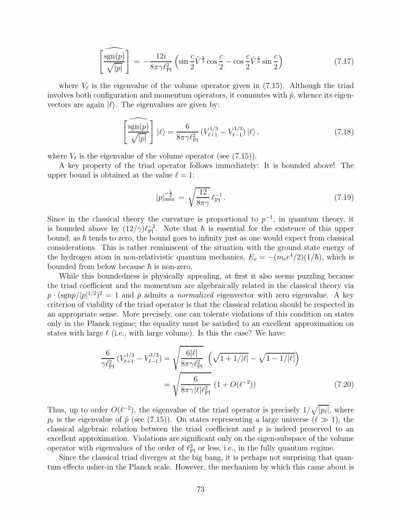
sgn(p)√|p|

]= − 12i

8πγℓ2Pl

(sin

c

2V

13 cos

c

2− cos

c

2V

13 sin

c

2

)(7.17)

where Vℓ is the eigenvalue of the volume operator given in (7.15). Although the triadinvolves both configuration and momentum operators, it commutes with p, whence its eigen-vectors are again |ℓ〉. The eigenvalues are given by:

[

sgn(p)√|p|

]|ℓ〉 =

6

8πγℓ2Pl

(V1/3ℓ+1 − V

1/3ℓ−1 ) |ℓ〉 . (7.18)

where Vℓ is the eigenvalue of the volume operator (see (7.15)).A key property of the triad operator follows immediately: It is bounded above! The

upper bound is obtained at the value ℓ = 1:

|p|−12

max =

√12

8πγℓ−1Pl . (7.19)

Since in the classical theory the curvature is proportional to p−1, in quantum theory, itis bounded above by (12/γ)ℓ−2

Pl . Note that ~ is essential for the existence of this upperbound; as ~ tends to zero, the bound goes to infinity just as one would expect from classicalconsiderations. This is rather reminiscent of the situation with the ground state energy ofthe hydrogen atom in non-relativistic quantum mechanics, Eo = −(mee

4/2)(1/~), which isbounded from below because ~ is non-zero.

While this boundedness is physically appealing, at first it also seems puzzling becausethe triad coefficient and the momentum are algebraically related in the classical theory viap · (sgnp/|p|1/2)2 = 1 and p admits a normalized eigenvector with zero eigenvalue. A keycriterion of viability of the triad operator is that the classical relation should be respected inan appropriate sense. More precisely, one can tolerate violations of this condition on statesonly in the Planck regime; the equality must be satisfied to an excellent approximation onstates with large ℓ (i.e., with large volume). Is this the case? We have:

6

γℓ2Pl

(V1/3ℓ+1 − V

1/3ℓ−1 ) =

√6|ℓ|

8πγℓ2Pl

(√1 + 1/|ℓ| −

√1 − 1/|ℓ|

)

=

√6

8πγ|ℓ|ℓ2Pl

(1 +O(ℓ−2)) (7.20)

Thus, up to order O(ℓ−2), the eigenvalue of the triad operator is precisely 1/√|pℓ|, where

pℓ is the eigenvalue of p (see (7.15)). On states representing a large universe (ℓ ≫ 1), theclassical algebraic relation between the triad coefficient and p is indeed preserved to anexcellent approximation. Violations are significant only on the eigen-subspace of the volumeoperator with eigenvalues of the order of ℓ3Pl or less, i.e., in the fully quantum regime.

Since the classical triad diverges at the big bang, it is perhaps not surprising that quan-tum effects usher-in the Planck scale. However, the mechanism by which this came about is

73

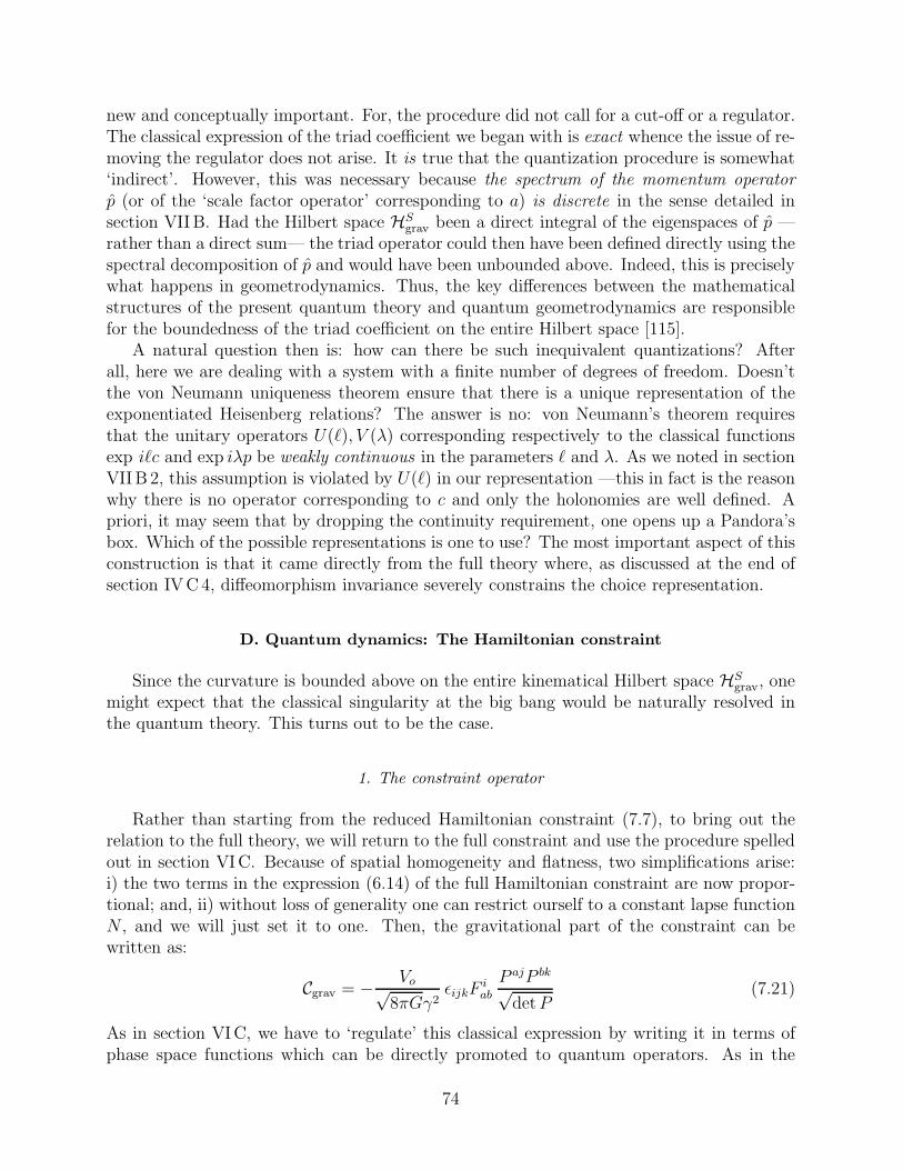
new and conceptually important. For, the procedure did not call for a cut-off or a regulator.The classical expression of the triad coefficient we began with is exact whence the issue of re-moving the regulator does not arise. It is true that the quantization procedure is somewhat‘indirect’. However, this was necessary because the spectrum of the momentum operatorp (or of the ‘scale factor operator’ corresponding to a) is discrete in the sense detailed insection VIIB. Had the Hilbert space HS

grav been a direct integral of the eigenspaces of p —rather than a direct sum— the triad operator could then have been defined directly using thespectral decomposition of p and would have been unbounded above. Indeed, this is preciselywhat happens in geometrodynamics. Thus, the key differences between the mathematicalstructures of the present quantum theory and quantum geometrodynamics are responsiblefor the boundedness of the triad coefficient on the entire Hilbert space [115].

A natural question then is: how can there be such inequivalent quantizations? Afterall, here we are dealing with a system with a finite number of degrees of freedom. Doesn’tthe von Neumann uniqueness theorem ensure that there is a unique representation of theexponentiated Heisenberg relations? The answer is no: von Neumann’s theorem requiresthat the unitary operators U(ℓ), V (λ) corresponding respectively to the classical functionsexp iℓc and exp iλp be weakly continuous in the parameters ℓ and λ. As we noted in sectionVIIB 2, this assumption is violated by U(ℓ) in our representation —this in fact is the reasonwhy there is no operator corresponding to c and only the holonomies are well defined. Apriori, it may seem that by dropping the continuity requirement, one opens up a Pandora’sbox. Which of the possible representations is one to use? The most important aspect of thisconstruction is that it came directly from the full theory where, as discussed at the end ofsection IVC4, diffeomorphism invariance severely constrains the choice representation.

D. Quantum dynamics: The Hamiltonian constraint

Since the curvature is bounded above on the entire kinematical Hilbert space HSgrav, one

might expect that the classical singularity at the big bang would be naturally resolved inthe quantum theory. This turns out to be the case.

1. The constraint operator

Rather than starting from the reduced Hamiltonian constraint (7.7), to bring out therelation to the full theory, we will return to the full constraint and use the procedure spelledout in section VIC. Because of spatial homogeneity and flatness, two simplifications arise:i) the two terms in the expression (6.14) of the full Hamiltonian constraint are now propor-tional; and, ii) without loss of generality one can restrict ourself to a constant lapse functionN , and we will just set it to one. Then, the gravitational part of the constraint can bewritten as:

Cgrav = − Vo√8πGγ2

ǫijkFiab

P ajP bk

√detP

(7.21)

As in section VIC, we have to ‘regulate’ this classical expression by writing it in terms ofphase space functions which can be directly promoted to quantum operators. As in the

74

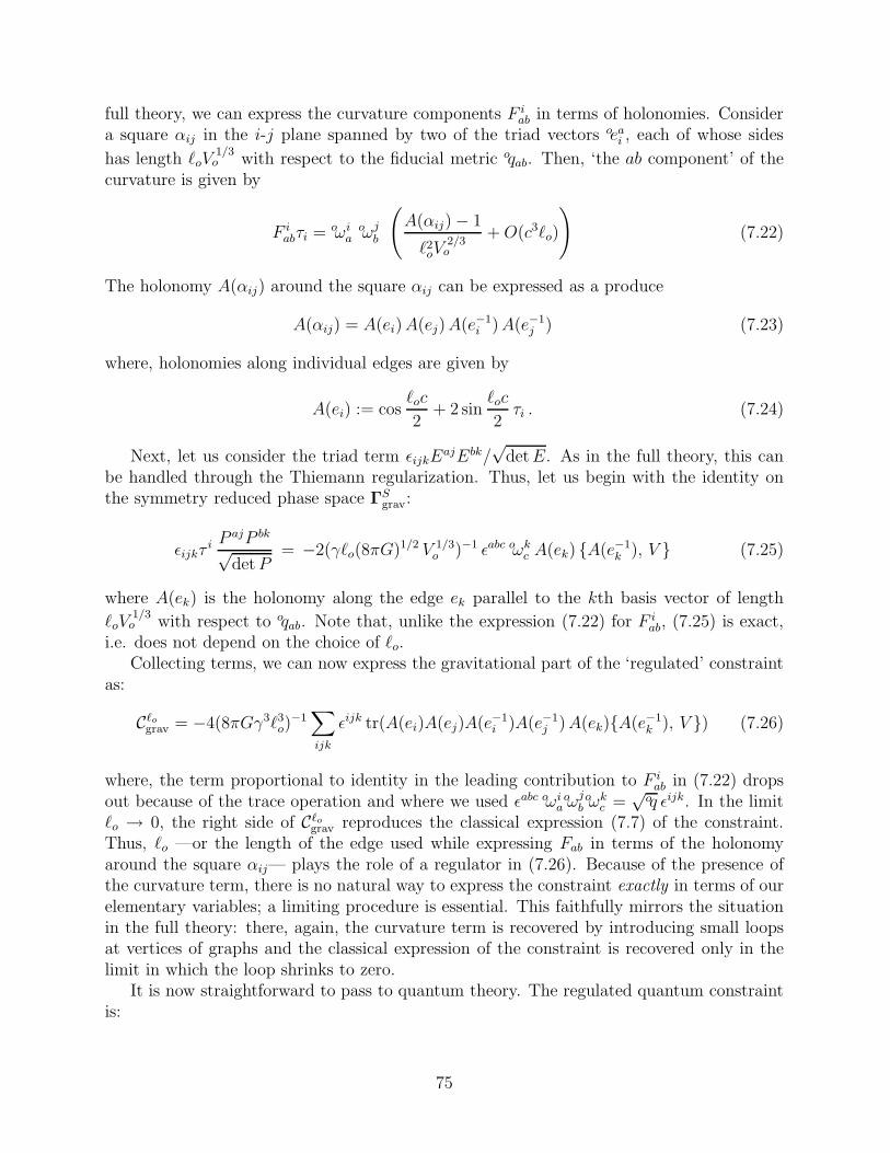
full theory, we can express the curvature components F iab in terms of holonomies. Consider

a square αij in the i-j plane spanned by two of the triad vectors oeai , each of whose sides

has length ℓoV1/3o with respect to the fiducial metric oqab. Then, ‘the ab component’ of the

curvature is given by

F iabτi = oωi

aoωj

b

(A(αij) − 1

ℓ2oV2/3o

+O(c3ℓo)

)(7.22)

The holonomy A(αij) around the square αij can be expressed as a produce

A(αij) = A(ei)A(ej)A(e−1i )A(e−1

j ) (7.23)

where, holonomies along individual edges are given by

A(ei) := cosℓoc

2+ 2 sin

ℓoc

2τi . (7.24)

Next, let us consider the triad term ǫijkEajEbk/

√detE. As in the full theory, this can

be handled through the Thiemann regularization. Thus, let us begin with the identity onthe symmetry reduced phase space ΓS

grav:

ǫijkτi P

ajP bk

√detP

= −2(γℓo(8πG)1/2 V 1/3o )−1 ǫabc oωk

c A(ek) A(e−1k ), V (7.25)

where A(ek) is the holonomy along the edge ek parallel to the kth basis vector of length

ℓoV1/3o with respect to oqab. Note that, unlike the expression (7.22) for F i

ab, (7.25) is exact,i.e. does not depend on the choice of ℓo.

Collecting terms, we can now express the gravitational part of the ‘regulated’ constraintas:

Cℓo

grav = −4(8πGγ3ℓ3o)−1∑

ijk

ǫijk tr(A(ei)A(ej)A(e−1i )A(e−1

j )A(ek)A(e−1k ), V ) (7.26)

where, the term proportional to identity in the leading contribution to F iab in (7.22) drops

out because of the trace operation and where we used ǫabc oωiaoωj

boωk

c =√

oq ǫijk. In the limitℓo → 0, the right side of Cℓo

grav reproduces the classical expression (7.7) of the constraint.Thus, ℓo —or the length of the edge used while expressing Fab in terms of the holonomyaround the square αij— plays the role of a regulator in (7.26). Because of the presence ofthe curvature term, there is no natural way to express the constraint exactly in terms of ourelementary variables; a limiting procedure is essential. This faithfully mirrors the situationin the full theory: there, again, the curvature term is recovered by introducing small loopsat vertices of graphs and the classical expression of the constraint is recovered only in thelimit in which the loop shrinks to zero.

It is now straightforward to pass to quantum theory. The regulated quantum constraintis:

75

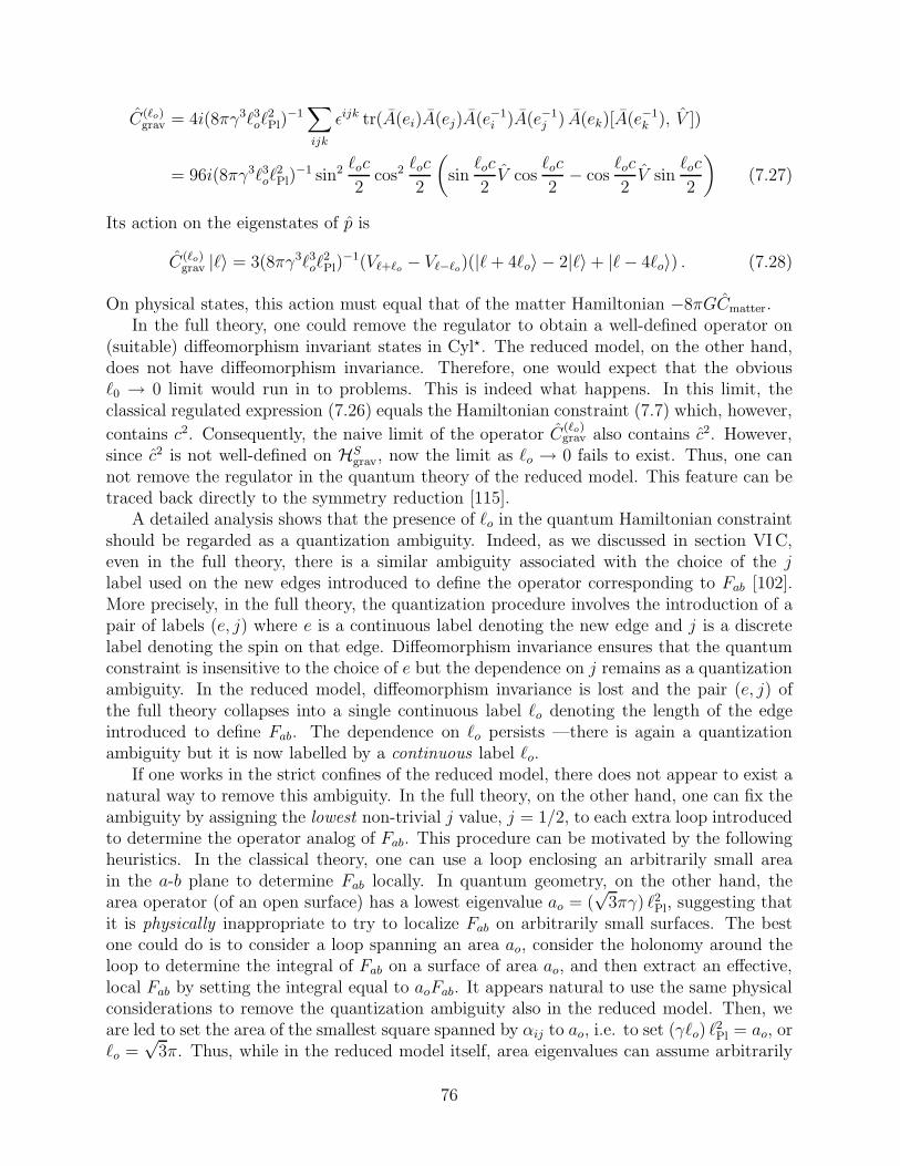
C(ℓo)grav = 4i(8πγ3ℓ3oℓ

2Pl)

−1∑

ijk

ǫijk tr(A(ei)A(ej)A(e−1i )A(e−1

j ) A(ek)[A(e−1k ), V ])

= 96i(8πγ3ℓ3oℓ2Pl)

−1 sin2 ℓoc

2cos2 ℓoc

2

(sin

ℓoc

2V cos

ℓoc

2− cos

ℓoc

2V sin

ℓoc

2

)(7.27)

Its action on the eigenstates of p is

C(ℓo)grav |ℓ〉 = 3(8πγ3ℓ3oℓ

2Pl)

−1(Vℓ+ℓo− Vℓ−ℓo

)(|ℓ+ 4ℓo〉 − 2|ℓ〉 + |ℓ− 4ℓo〉) . (7.28)

On physical states, this action must equal that of the matter Hamiltonian −8πGCmatter.In the full theory, one could remove the regulator to obtain a well-defined operator on

(suitable) diffeomorphism invariant states in Cyl⋆. The reduced model, on the other hand,does not have diffeomorphism invariance. Therefore, one would expect that the obviousℓ0 → 0 limit would run in to problems. This is indeed what happens. In this limit, theclassical regulated expression (7.26) equals the Hamiltonian constraint (7.7) which, however,

contains c2. Consequently, the naive limit of the operator C(ℓo)grav also contains c2. However,

since c2 is not well-defined on HSgrav, now the limit as ℓo → 0 fails to exist. Thus, one can

not remove the regulator in the quantum theory of the reduced model. This feature can betraced back directly to the symmetry reduction [115].

A detailed analysis shows that the presence of ℓo in the quantum Hamiltonian constraintshould be regarded as a quantization ambiguity. Indeed, as we discussed in section VIC,even in the full theory, there is a similar ambiguity associated with the choice of the jlabel used on the new edges introduced to define the operator corresponding to Fab [102].More precisely, in the full theory, the quantization procedure involves the introduction of apair of labels (e, j) where e is a continuous label denoting the new edge and j is a discretelabel denoting the spin on that edge. Diffeomorphism invariance ensures that the quantumconstraint is insensitive to the choice of e but the dependence on j remains as a quantizationambiguity. In the reduced model, diffeomorphism invariance is lost and the pair (e, j) ofthe full theory collapses into a single continuous label ℓo denoting the length of the edgeintroduced to define Fab. The dependence on ℓo persists —there is again a quantizationambiguity but it is now labelled by a continuous label ℓo.

If one works in the strict confines of the reduced model, there does not appear to exist anatural way to remove this ambiguity. In the full theory, on the other hand, one can fix theambiguity by assigning the lowest non-trivial j value, j = 1/2, to each extra loop introducedto determine the operator analog of Fab. This procedure can be motivated by the followingheuristics. In the classical theory, one can use a loop enclosing an arbitrarily small areain the a-b plane to determine Fab locally. In quantum geometry, on the other hand, thearea operator (of an open surface) has a lowest eigenvalue ao = (

√3πγ) ℓ2Pl, suggesting that

it is physically inappropriate to try to localize Fab on arbitrarily small surfaces. The bestone could do is to consider a loop spanning an area ao, consider the holonomy around theloop to determine the integral of Fab on a surface of area ao, and then extract an effective,local Fab by setting the integral equal to aoFab. It appears natural to use the same physicalconsiderations to remove the quantization ambiguity also in the reduced model. Then, weare led to set the area of the smallest square spanned by αij to ao, i.e. to set (γℓo) ℓ

2Pl = ao, or

ℓo =√

3π. Thus, while in the reduced model itself, area eigenvalues can assume arbitrarily

76

small values, if one ‘imports’ from the full theory the value of the smallest non-zero areaeigenvalue, one is naturally led to set ℓo =

√3π.

To summarize, in loop quantum cosmology, one adopts the viewpoint that (7.27), withℓo =

√3π, is the ‘fundamental’ Hamiltonian constraint operator which ‘correctly’ incorpo-

rates the underlying discreteness of quantum geometry and the classical expression (7.7)is an approximation which is valid only in regimes where this discreteness can be ignoredand the continuum picture is valid. This viewpoint is borne out by detailed calculations[115]: the expectation values of Cℓo

grav in semi-classical states reproduce the classical con-straint. Furthermore, one can calculate corrections to the classical expression arising fromthe fundamental discreteness and quantum fluctuations inherent in the semi-classical quan-tum states [117].

2. Physical states

Let us now solve the quantum constraint and obtain physical states. For simplicity, weassume that the matter is only minimally coupled to gravity (i.e., there are no curvaturecouplings). As in non-trivially constrained systems, one expects that the physical stateswould fail to be normalizable in the kinematical Hilbert space HS = HS

grav ⊗ HSmatter (see,

e.g., [88,89]). However, as in the full theory, they do have a natural ‘home’. We again havea triplet

CylS ⊂ HS ⊂ Cyl⋆S

of spaces and physical states will belong to Cyl⋆S, the algebraic dual of CylS. Since elementsof Cyl⋆S need not be normalizable, as in section VIC, we will denote them by (Ψ|. (Theusual, normalizable bras will be denoted by 〈Ψ|.)

It is convenient to exploit the existence of a triad representation. Then, every element(Ψ| of Cyl⋆S can be expanded as

(Ψ| =∑

ℓ

ψ(φ, ℓ)〈ℓ| (7.29)

where φ denotes the matter field and 〈ℓ| are the (normalized) eigenbras of p. Note thatthe sum is over a continuous variable ℓ whence (Ψ| need not be normalizable. Now, theconstraint equation

(Ψ|(C(ℓo)

grav + 8πGC(ℓo)matter

)†= 0 (7.30)

turns into the equation

(Vℓ+5ℓo− Vℓ+3ℓo

)ψ(φ, ℓ+ 4ℓo) − 2(Vℓ+ℓo− Vℓ−ℓo

)ψ(φ, ℓ)

+ (Vℓ−3ℓo− Vℓ−5ℓo

)ψ(φ, ℓ− 4ℓo) = −1

38πGγ3ℓ3oℓ

2Pl C

(ℓo)matter(ℓ)ψ(φ, ℓ) (7.31)

for the coefficients ψ(φ, ℓ), where C(ℓo)matter(ℓ) only acts on the matter fields (and depends on ℓ

via metric components in the matter Hamiltonian). Note that, even though ℓ is a continuousvariable, the quantum constraint is a difference equation rather than a differential equation.

77

Strictly, (7.31) just constrains the coefficients ψ(φ, ℓ) to ensure that (Ψ| is a physical state.As in the full quantum theory, we do not have a background space-time, hence no naturalnotion of ‘time’ or ‘evolution’. However, since each 〈ℓ| is an eigenbra of the volume operator,it tells us how the matter wave function is correlated with volume, i.e., geometry. Now, if onewishes, one can regard p as providing a heuristic ‘notion of time’, and then think of (7.31)as an evolution equation for the quantum state of matter with respect to this time. (Notethat p goes from −∞ to ∞, negative values corresponding to triads which are oppositelyoriented to the fiducial one. The classical big-bang corresponds to p = 0.) This heuristicinterpretation often provides physical intuition for (7.31); one can regard it as a discrete‘evolution’ equation. However, it is not essential for what follows; one can forego thisinterpretation entirely and regard (7.31) only as a constraint equation.

What is the fate of the classical singularity? At the big bang, the scale factor goes tozero. Hence it corresponds to the state |ℓ = 0〉 in HS

grav. So, the key question is whether thequantum ‘evolution’ breaks down at ℓ = 0. Let us examine this issue. Starting at ℓ = −4Nℓofor some large positive N , and fixing values of ψ(φ,−4Nℓo) and ψ(φ, (−4N +4)ℓo), one canuse the equation to determine the coefficients ψ(φ, (−4N + 4n)ℓ0) for all n > 1, providedthe coefficient of the highest order term in (7.31) continues to remain non-zero. Now, itis easy to verify that the coefficient vanishes if and only if n = N . Thus, the coefficientψ(φ, ℓ = 0) remains undetermined. In its place, one just obtains a consistency conditionconstraining the coefficients ψ(φ, ℓ=−4) and ψ(φ, ℓ=−8). Now, since ψ(φ, ℓ= 0) remainsundetermined, at first sight, it may appear that one can not ‘evolve’ past the singularity, i.e.that the quantum evolution also breaks down at the big-bang. However, the main point isthat this is not the case. For, the structure of the quantum scalar constraint is such that thecoefficient ψ(φ, ℓ= 0) just decouples from the rest. This comes about because of two facts:i) the minimally coupled matter Hamiltonians annihilate ψ(φ, ℓ= 0) = 0 [104,110]; and ii)Vℓo

= V−ℓo. Thus, unlike in the classical theory, evolution does not stop at the singularity;

the difference equation (7.31) lets us ‘evolve’ right through it. In this analysis, we started atℓ = −4Nℓo because we wanted to test what happens if one encounters the singularity ‘headon’. If one begins at a generic ℓ, the ‘discrete evolution’ determined by (7.31) just ‘jumps’over the classical singularity without encountering any subtleties.

Next, let us consider the space of solutions. An examination of the classical degreesof freedom suggests that the freedom in physical quantum states should correspond to twofunctions just of matter fields φ. The space of solutions to the Hamiltonian constraint, onthe other hand is much larger: there are as many solutions as there are functions ψ(φ, ℓ) onan interval [ℓ′−4ℓo, ℓ

′+4ℓo), where ℓ′ is any fixed number. Thus suggests that a large numberof these solutions may be redundant. Indeed, to complete the quantization procedure, oneneeds to introduce an appropriate inner product on the space of solutions to the Hamiltonianconstraint. The physical Hilbert space is then spanned by just those solutions to the quantumconstraint which have finite norm. In simple examples one generally finds that, while thespace of solutions to all constraints can be very large, the requirement of finiteness of normsuffices to produce a Hilbert space of the physically expected size.

For the reduced system considered here, one have a quantum mechanical system andwith a single constraint in quantum cosmology. Hence it should be possible to extractphysical states using the group averaging technique of the ‘refined algebraic framework’[88,89]. However, this analysis is yet to be carried out explicitly and therefore one does not

78

yet have a good control on how large the physical Hilbert space really is. This issue is beinginvestigated.

To summarize, two factors were key to the resolution of the big bang singularity: i) asa direct consequence of quantum geometry, the Hamiltonian constraint is now a differenceequation rather than a differential equation as in geometrodynamics; and ii) the coefficientsin the difference equation are such that one can evolve unambiguously ‘through’ the sin-gularity even though the coefficient ψ(φ, ℓ = 0) is undetermined. Both these features arerobust: they are largely insensitive to factor ordering ambiguities and persist in more com-plicated cosmological models [111,113,116]. The qualitative changes introduced by quantumgeometry in kinematics and dynamics are significant only in the Planck regime. A carefulanalysis shows that the discrete evolution is extremely well approximated by the WheelerDeWitt differential equation at scales larger than ℓo in a precise sense [115]. Thus the fun-damental discreteness, characteristic of loop quantum gravity, intervenes in a subtle wayprecisely in the Planck regime where geometrodynamics fails to resolve singularities. Sinceloop quantum cosmology mimics the full theory as closely as possible, within the limitationsdiscussed at the very beginning of section VII, these results provide support for the approachto quantum dynamics in the full theory.

VIII. APPLICATIONS: QUANTUM GEOMETRY OF ISOLATED HORIZONS

AND BLACK HOLE ENTROPY

Loop quantum cosmology illuminates dynamical ramifications of quantum geometry butwithin the limited context of mini-superspaces where all but a finite number of degrees offreedom are frozen. In this section, we will discuss a complementary application whereone considers the full theory but probes consequences of quantum geometry which are notsensitive to the details of how the Hamiltonian constraint is imposed. (For further details,see [127–129,133–137,139]. For early work, see [122–124].)

As was explained in section I, since mid-seventies, a key question in the subject has been:What is the statistical mechanical origin of the black hole entropy SBH = (ahor/4ℓ

2Pl)? What

are the microscopic degrees of freedom that account for this entropy? This relation impliesthat a solar mass black hole must have (exp 1077) quantum states, a number that is huge evenby the standards of statistical mechanics. Where do all these states reside? To answer thesequestions, in the early nineties Wheeler [140] had suggested the following heuristic picture,which he christened ‘It from Bit ’. Divide the black hole horizon in to elementary cells, eachwith one Planck unit of area, ℓ2Pl and assign to each cell two microstates. Then the totalnumber of states N is given by N = 2n where n = (ahor/ℓ

2Pl) is the number of elementary

cells, whence entropy is given by S = lnN ∼ ahor. Thus, apart from a numerical coefficient,the entropy (‘It ’) is accounted for by assigning two states (‘Bit ’) to each elementary cell.This qualitative picture is simple and attractive. Thus, one is led to ask: can these heuristicideas be supported by a systematic analysis from first principles? What is the origin ofthe ‘elementary cells’? Why is each cell endowed with precisely two states? And mostimportantly: what has all this to do with a black hole? The ‘It from Bit’ considerationsseem to apply to any 2-surface! Quantum geometry enables one to address all these issuesin detail.

79

The precise picture is much more involved: because the area spectrum is quite com-plicated in quantum geometry, ‘elementary cells’ need not all carry the same area and thenumber of ‘internal states’ of each cell is also not restricted to two. Nonetheless, it doesturn out that a dominant contribution in the entropy calculation comes from states envis-aged by Wheeler. The purpose of this section is to summarize the overall situation. Ourdiscussion is divided in to three parts. In the first, we recall the ‘isolated horizon framework’in classical general relativity which serves as a point of departure for quantum theory. Inthe second we discuss the quantum geometry of the simplest (undistorted and non-rotating)horizons and present the entropy calculation allowing for the presence of minimally coupledmatter. In the third, we discuss extensions that include non-minimal couplings, distortionsand rotation.

A. Isolated horizons

A systematic approach to the problem of entropy requires that we first specify the classof horizons of interest. Since the entropy formula is expected to hold unambiguously forblack holes in equilibrium, most analyses were confined to stationary, eternal black holes(i.e., to the Kerr-Newman family in 4-dimensional general relativity). From a physical view-point however, this assumption seems overly restrictive. After all, in statistical mechanicalcalculations of entropy of ordinary systems, one only has to assume that the given systemis in equilibrium, not the whole world. Therefore, it should suffice for us to assume thatthe black hole itself is in equilibrium; the exterior geometry should not be forced to betime-independent. Furthermore, the analysis should also account for entropy of black holeswhich may be distorted or carry (Yang-Mills and other) hair. Finally, it has been knownsince the mid-seventies that the thermodynamical considerations apply not only to blackholes but also to cosmological horizons [121]. A natural question arises: Can these diversesituations be treated in a single stroke? In classical general relativity, the isolated horizonframework provides a natural avenue by encompassing all these situations. It also providesa Hamiltonian framework which serves as a natural point of departure for quantization[128,133,134]

Let us begin with the basic definitions [133]. In this discussion, we need to begin witha 4-dimensional space-time manifold M although we will return to 3-manifolds M once wehave a Hamiltonian framework.

A non-expanding horizon ∆ is a null, 3-dimensional sub-manifold of the 4-dimensionalspace-time (M, gαβ), with topology S2 ×R, such that:i) the expansion θℓ of its null normal ℓ vanishes; and,ii) Field equations hold on ∆ with stress energy, Tαβ , satisfying the very weak requirementthat −T α

βℓβ is a future-directed, causal vector. (Throughout, ℓα will be assumed to be

future pointing.)Note that: i) if the expansion vanishes for one null normal, it vanishes for all; and, ii) thecondition on stress energy is satisfied by all the standard matter fields provided they areminimally coupled to gravity.

The definition ensures that the area of any 2-sphere cross-section of the horizon is con-stant and matter flux across ∆ vanishes. It also implies that the space-time derivative

80

operator ∇ naturally induces a unique derivative operator D on ∆. Since ∆ is a null 3-surface, it has a degenerate intrinsic ‘metric’ qab of signature 0,+,+. The pair (qab,D) isreferred to as the geometry of ∆. The notion that the black hole itself is in equilibrium iscaptured by requiring that this geometry is time independent:

An isolated horizon (∆, ℓ) is a non-expanding horizon ∆ equipped with a null normal ℓsuch that ℓ is a symmetry of the geometry; i.e., Lℓqab = 0 and [Lℓ, D] = 0 on ∆.One can show that, generically, the null normal ℓ satisfying these conditions is unique up toa constant rescaling. For simplicity, we will assume that we are in the generic case althoughthe main results go through in all cases.

The isolated horizon definition extracts from the notion of the Killing horizon just that‘tiny’ part which turns out to be essential for black hole mechanics and, more generally, tocapture the notion that the horizon is in equilibrium, allowing for dynamical processes andradiation in the exterior region. Indeed, Einstein’s equations admit solutions with isolatedhorizons in which there is radiation arbitrarily close to the horizons [131,132]. Note that inthe definition uses conditions which are local to ∆. Thus, unlike event horizons, this notionis local, not ‘teleological’. For our purposes, the two important considerations are:i) The definition is satisfied not only by event horizons of stationary black holes but alsoby the standard cosmological horizons. Thus, all situations in which thermodynamicalconsiderations apply are treated in one stroke.ii) If one restricts oneself to space-times which admit an internal boundary which is anisolated horizon, the action principle and the Hamiltonian description is well-defined andthe resulting phase space has an infinite number of degrees of freedom. This would not bethe case if one used general event horizons or Killing horizons instead.

Next, let us examine symmetry groups of isolated horizons. A symmetry of (∆, ℓ, q,D)is a space-time diffeomorphism which maps ∆ to itself; at most rescales ℓ by a constant,and preserves q and D. It is clear the diffeomorphisms generated by any smooth extensionof ℓα are symmetries. So, the symmetry group G∆ is at least 1-dimensional. The questionis: Are there any other symmetries? At infinity, we generally have a universal symmetrygroup (such as the Poincare or the anti-de Sitter) because all metrics under considerationapproach a fixed metric (Minkowskian or anti-de Sitter) there. In the case of the isolatedhorizons, generically we are in the strong field regime and space-time metrics do not ap-proach a universal metric. Therefore, the symmetry group is not universal. However, thereare only three universality classes:i) Type I: the isolated horizon geometry is spherical; in this case, G∆ is four dimensional;ii) Type II: the isolated horizon geometry is axi-symmetric; in this case, G∆ is two dimen-sional;iii) Type III: the diffeomorphisms generated by ℓα are the only symmetries; G∆ is onedimensional.

Note that these symmetries refer only to the horizon geometry. The full space-time metricneed not admit any isometries even in a neighborhood of the horizon. Physically, type IIhorizons are the most interesting ones. They include the Kerr-Newman horizons as well astheir generalizations incorporating distortions (to due exterior matter of other black holes)and hair. The zeroth and the first laws of black hole mechanics can be naturally extendedto type II isolated horizons [133,134]. In particular, for the Einstein-Maxwell theory, onecan define the mass M∆ and angular momentum J∆ of the horizon using only the intrinsic

81

geometry of the isolated horizon and show that the first law holds:

dM∆ =κ

8πGda∆ + ΩdJ∆ + ΦdQ∆ (8.1)

where κ,Ω,Φ are, respectively, the surface gravity, angular velocity and the electric potentialat the horizon and d denotes the exterior derivative on the (infinite dimensional) phase space.This law of isolated horizon mechanics encompasses all black holes and cosmological horizonsin equilibrium, including the ones which arbitrary distortion and rotation.

B. Type I isolated horizons: Quantum theory

Let us first discuss type I isolated horizons in detail and then generalize the resultsto include non-minimally coupled matter and type II horizons. We will divide the type Idiscussion in to three parts. In the first, we introduce the Hamiltonian formulation; in thesecond, we describe the quantum horizon geometry; and in the third, we summarize theentropy calculation.

1. Hamiltonian framework

Consider the sector of general relativity consisting of gravitational and matter fields forwhich the underlying space-time admits an internal boundary which is a type I isolatedhorizon ∆ with a fixed area ao. We will focus on geometrical structures near ∆ and onthe modifications of the Hamiltonian framework of section II caused by the presence of aninternal boundary.

Denote by S the 2-sphere intersection of the (partial) Cauchy surface M with the isolatedhorizon ∆. Introduce on ∆ an internal vector field ri, i.e. any isomorphism from the unit2-sphere in the Lie algebra of SU(2) to S and partially gauge fix the internal SU(2) freedomto U(1) by requiring that riP a

i =√

| det q| ra, where ra is the unit normal to S. Then it turnsout that the intrinsic geometry of ∆ is completely determined by the pull-back Airi =: 2Wto S of the connection Ai on M [135]. Furthermore, W is in fact a spin-connection intrinsicto the 2-sphere S: W = 1

2Airi = 1

2Γiri on S (see (2.20). Thus, if we consider orthonormal

dyads (m, m) on S with internal rotation freedom in SO(2), W is a connection on thecorresponding U(1) bundle. Now, this U(1) bundle on S is non-trivial and

∮SdW equals

−2π, rather than zero. (But since the Chern class of any spin connection is the same,∮SδW = 0; tangent vectors δW to the phase space are genuine 1-forms, globally defined on

S. This fact will be useful in the discussion of the symplectic structure.) Finally, the factthat S is (the intersection of M with) a type I isolated horizon is captured in a relationbetween the two canonically conjugate fields:

F := dW = −2π

ao

8πGγ Σi ri. (8.2)

where Σi is the pull-back to S of the 2-forms Σiab = ηabcP

aj η

ij on M , dual to the momentumP a

i . Thus, because of the isolated horizon boundary conditions, fields which would otherwise

82

be independent are now related. As one would expect, the boundary conditions reduce thenumber of independent fields; in particular, the pull-backs to S of the canonically conjugatefields Ai

a,Σiab are completely determined by the U(1) connection W .

The main modification in the Hamiltonian framework of section II is that the gravita-tional symplectic structure now acquires a surface term:

Ω(δ1, δ2) = −∫

M

Tr (δ1A ∧ δ2Σ − δ2A ∧ δ1Σ) +1

2π

ao

4πGγ

∮

S

δ1W ∧ δ2W , (8.3)

where, as in section II, δ ≡ (δA, δΣ) denote tangent vectors to the phase space Γ. Since Wis essentially the only ‘free data’ on the horizon, it is not surprising that the surface termof the symplectic structure is expressible entirely in terms of W . However, it is interestingand somewhat surprising that the new surface term is precisely the symplectic structure ofthe U(1)-Chern Simons theory. The symplectic structures of the Maxwell, Yang-Mills, scalarand dilatonic fields do not acquire surface terms. Conceptually, this is an important point:this, in essence, is the reason why (for minimally coupled matter) the black hole entropydepends just on the area and not, in addition, on the matter charges.

2. Quantum horizon geometry

In the classical theory, the bulk fields determine the surface fields just by continuity; thereare no independent degrees of freedom on the surface in the classical phase space. In thequantum theory, on the other hand the fields are distributional and arbitrarily discontinuouswhence the surface and the bulk fields effectively decouple. It is this phenomenon that isresponsible for creating ‘independent surface states’ in the quantum theory.

The main task is to extend the ‘bulk’ quantum geometry of sections IV and V to allowfor the presence of an internal boundary S. Now, the space of generalized connections A is aproduct A = AV ×AS, where a volume generalized connection AV assigns an SU(2) elementto any (closed-piecewise analytic) edge lying in the bulk while AS assigns an U(1) elementto each (closed-piecewise analytic) edge lying in the surface S. Therefore, it is natural tobegin with a total Hilbert space H = HV ⊗ HS where HV is built from suitable functionsof generalized connections in the bulk and HS from suitable functions of generalized surfaceconnections. The volume Hilbert space HV is the one that comes from bulk quantum ge-ometry of section IV: HV = L2(A, µo). The question is: What would be the surface Hilbertspace? The answer is suggested by the structure of the surface term in the symplectic struc-ture: It should be the Hilbert space of Chern-Simons theory on the horizon. Furthermore,the coefficient in front of this surface term tells us that the quantum Chern-Simons theorymust have a (dimensionless) coupling constant/level k given by:

k =ao

4πγℓ2Pl

(8.4)

But we also have to incorporate the boundary condition (8.2) which ensures that S is not anyold 2-surface but an isolated horizon. The key idea is to impose it quantum mechanically,as an operator equation on H, i.e. via

83

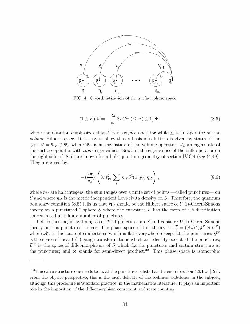
n-1

n-1

n-1

2p1

p p3

p pn

γ1 2 γ3 γ

η1 η2 η3 η

γ

FIG. 4. Co-ordinatization of the surface phase space

(1 ⊗ F ) Ψ = −2π

ao8πGγ (Σ · r) ⊗ 1) Ψ , (8.5)

where the notation emphasizes that F is a surface operator while Σ is an operator on thevolume Hilbert space. It is easy to show that a basis of solutions is given by states of thetype Ψ = ΨV ⊗ ΨS where ΨV is an eigenstate of the volume operator, ΨS an eigenstate ofthe surface operator with same eigenvalues. Now, all the eigenvalues of the bulk operator onthe right side of (8.5) are known from bulk quantum geometry of section IVC4 (see (4.49).They are given by:

− (2π

ao)

(8πℓ2Pl

∑

I

mI δ3(x, pI) ηab

), (8.6)

where mI are half integers, the sum ranges over a finite set of points —called punctures— onS and where ηab is the metric independent Levi-civita density on S. Therefore, the quantumboundary condition (8.5) tells us that HS should be the Hilbert space of U(1)-Chern-Simonstheory on a punctured 2-sphere S where the curvature F has the form of a δ-distributionconcentrated at a finite number of punctures.

Let us then begin by fixing a set P of punctures on S and consider U(1)-Chern-Simonstheory on this punctured sphere. The phase space of this theory is ΓP

S = (AoS)/(GP ⋊ DP)

where AoS is the space of connections which is flat everywhere except at the punctures; GP

is the space of local U(1) gauge transformations which are identity except at the punctures;DP is the space of diffeomorphisms of S which fix the punctures and certain structure atthe punctures; and ⋊ stands for semi-direct product.30 This phase space is isomorphic

30The extra structure one needs to fix at the punctures is listed at the end of section 4.3.1 of [129].

From the physics perspective, this is the most delicate of the technical subtleties in the subject,

although this procedure is ‘standard practice’ in the mathematics literature. It plays an important

role in the imposition of the diffeomorphism constraint and state counting.

84

with the torus T2(n−1) if there are n punctures in the set P, equipped with the naturalsymplectic structure on T2(n−1). A convenient set of canonically conjugate coordinates canbe introduced as follows. Let us fix the nth puncture as ‘origin’ and, as in Fig 4, denote byγI , a family of curves joining the Ith puncture to the nth, (with I = 1, 2, . . . , n− 1)) and byηI , ‘small’ closed loops surrounding each of the first n− 1 punctures. Then, for each I, twoholonomies around γI and ηI are canonically conjugate. This phase space is often referredto as the non-commutative torus.

The Hilbert space HPS of surface states results from geometric quantization of this torus

[129]. This is the space of quantum states of the U(1) Chern-Simons theory on (S,P).The total surface Hilbert space HS is the inductive limit of these Hilbert spaces as theset P becomes larger and larger. As discussed in section IV, the volume Hilbert spaceHV = L2(Av, dµo) can also be obtained as the inductive limit of the Hilbert spaces (HV )α

associated with graphs α [44,45,66].Next one has to impose the quantum boundary condition (8.5). This introduces a highly

non-trivial test of the whole framework. Construction of the surface Hilbert space wasstrongly motivated by (8.5). However, now that it is complete, there is no more freedom. Inthe Chern-Simons Hilbert space, one can compute the eigenvalues of the surface operator F .This calculation is completely independent of the volume Hilbert space; it has never heardof the quantum geometry in the bulk. The key question on which everything hinges is: Arethe eigenvalues of F the same as the eigenvalues (8.6) of the bulk operator in (8.5)? If not,there will be no solutions to the quantum boundary conditions! The remarkable fact is thatthe infinite set of eigenvalues of the two operators match, even though the two calculationsare completely distinct. This comes about because the level of the Chern-Simons theory isrelated to the Barbero-Immirzi parameter γ and the area ao in a very specific way, which inturn is a consequence of the isolated horizon boundary conditions. Thus there is a seamlessmatching between three completely independent theories: the isolated horizon framework inclassical general relativity; the bulk quantum geometry; and, the Chern-Simons theory onthe punctured horizon. And this matching provides a coherent mathematical description ofthe quantum geometry of the horizon.

Finally, one has to impose quantum Einstein’s equations. The Gauss constraint asksthat the total state ΨV ⊗ΨS should be gauge invariant. The diffeomorphism constraint asksthat diffeomorphisms on S should be regarded as gauge. Again there are important math-ematical subtleties. But the final picture is simple. While each of the bulk and the surfacestates transforms non-trivially under the remaining gauge freedom (G/GP), the total stateis gauge invariant as needed. Implementation of the remaining diffeomorphism constraint(corresponding to D/DP) asks that what matters is only the number of punctures; theirlocation is irrelevant.31

31The subtleties are: i) In the Chern-Simons theory, only the exponentiated operator exp iF

is well-defined; F itself is not. Therefore, the mathematically meaningful quantum boundary

condition is the exponentiated version of (8.5). ii) the U(1) gauge group at the punctures is

replaced by the quantum U(1) group. The deformation parameter is supplied by the level k

of the Chern-Simons theory which is required to be an integer because of the pe-quantization

85

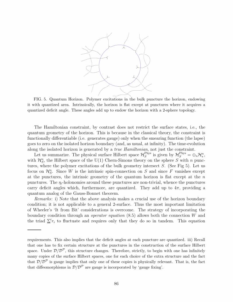
FIG. 5. Quantum Horizon. Polymer excitations in the bulk puncture the horizon, endowing

it with quantized area. Intrinsically, the horizon is flat except at punctures where it acquires a

quantized deficit angle. These angles add up to endow the horizon with a 2-sphere topology.

The Hamiltonian constraint, by contrast does not restrict the surface states, i.e., thequantum geometry of the horizon. This is because in the classical theory, the constraint isfunctionally differentiable (i.e. generates gauge) only when the smearing function (the lapse)goes to zero on the isolated horizon boundary (and, as usual, at infinity). The time-evolutionalong the isolated horizon is generated by a true Hamiltonian, not just the constraint.

Let us summarize. The physical surface Hilbert space HPhysS is given by HPhys

S = ⊕nHns ,

with HnS, the Hilbert space of the U(1) Chern-Simons theory on the sphere S with n punc-

tures, where the polymer excitations of the bulk geometry intersect S. (See Fig 5). Let usfocus on Hn

S. Since W is the intrinsic spin-connection on S and since F vanishes exceptat the punctures, the intrinsic geometry of the quantum horizon is flat except at the npunctures. The ηi-holonomies around these punctures are non-trivial, whence the puncturescarry deficit angles which, furthermore, are quantized. They add up to 4π, providing aquantum analog of the Gauss-Bonnet theorem.

Remarks : i) Note that the above analysis makes a crucial use of the horizon boundarycondition; it is not applicable to a general 2-surface. Thus the most important limitationof Wheeler’s ‘It from Bit’ considerations is overcome. The strategy of incorporating theboundary condition through an operator equation (8.5) allows both the connection W andthe triad Σiri to fluctuate and requires only that they do so in tandem. This equation

requirements. This also implies that the deficit angles at each puncture are quantized. iii) Recall

that one has to fix certain structure at the punctures in the construction of the surface Hilbert

space. Under D/DP , this structure changes. Therefore, strictly, to begin with one has infinitely

many copies of the surface Hilbert spaces, one for each choice of the extra structure and the fact

that D/DP is gauge implies that only one of these copies is physically relevant. That is, the fact

that diffeomorphisms in D/DP are gauge is incorporated by ‘gauge fixing’.

86

provides the first step in the answer to the question: what is a quantum black hole?ii) For extensions of this framework to include non-minimally coupled fields and type

II horizons (discussed in section VIIIC), let us note that there are just three essentialmathematical ingredients which serve as the input for this construction of the surface Hilbertspace: a) the form of the surface term in (8.3) which shows that the surface symplecticstructure is that of the U(1)-Chern-Simons theory with level k of (8.4); b) the horizonboundary condition (8.2); and c) The spectrum (8.6) of the triad operator Σiri.

3. Entropy: Counting surface states

In the classical theory, ao in the expression of the surface term of the symplectic structure(8.3) and in the boundary condition (8.2) is the horizon area. However in the quantum theory,ao has simply been a parameter so far; we have not tied it to the physical area of the horizon.To calculate entropy, one has to construct a suitable ‘micro-canonical’ ensemble by relatingao to the physical area.

It follows from the definition of volume connections that, as depicted in Fig 5, the poly-mer excitations of the bulk geometry puncture the horizon transversely from the ‘exterior’.Hence, the relevant area eigenvalues are those given in (5.18):

8πγℓ2Pl

∑

I

√jI(jI + 1) .

Therefore, one is led to construct the micro-canonical ensemble by considering only thatsub-space of the bulk theory which, at the horizon, satisfies:

ao − ǫ ≤ 8πγℓ2Pl

∑

I

√jI(jI + 1) ≤ ao + ǫ (8.7)

where I ranges over the number of punctures, jI is the spin label (the eigenvalue of thevertex operator JpI

associated with the puncture pI), and ℓ2Pl < ǫ ≪ a0). In presence of

matter fields carrying charges, one fixes values of horizon charges Q(α)o (labelled by α) and

restrict the matter configurations so that

Q(α)o − ǫ(α) ≤ Q(α)

o ≤ Q(α)o + ǫ(α) (8.8)

for suitably chosen ǫ(α). (As is usual in statistical mechanics, the leading contributionto the entropy is independent of the precise choice of these small intervals.) Now, thephysical states belonging to this ensemble contain information also about gravitational andelectromagnetic radiation far away from the horizon which is obviously irrelevant to thecalculation of black hole entropy. What is relevant are the states directly associated withthe horizon of a given area ao, and charges Q

(α)o . One is therefore led to trace over the

volume degrees of freedom and construct a density matrix ρ∆ describing a maximum entropymixture of surface satisfying (8.7) and (8.8). The statistical mechanical entropy is then givenby S∆ = −Tr(ρ∆ ln ρ∆). As usual, this number can be calculated simply by counting states:

S∆ = lnN∆ (8.9)

87

where N∆ is the number of Chern-Simons surface states consistent with the area and chargeconstraints. A detailed analysis [129], estimates this number and leads to the expression ofentropy of large black holes:

S∆ := lnN∆ =γo

γ

ao

4ℓ2Pl

+ o(ℓ2Pl

ao

), where γo =ln 2√3π

(8.10)

Thus, ignoring terms o(ℓ2Pl

ao), entropy is indeed proportional to the horizon area. However,

even for large black holes, one obtains agreement with the Hawking-Bekenstein formula onlyin the sector of quantum geometry in which the Barbero-Immirzi parameter γ takes thevalue γ = γo. Thus, while all γ sectors are equivalent classically, the standard quantum fieldtheory in curved space-times is recovered in the semi-classical theory only in the γo sector ofquantum geometry. It is quite remarkable that thermodynamical considerations involvinglarge black holes can be used to fix the quantization ambiguity which dictates such Planckscale properties as eigenvalues of geometric operators.

Now, the value of γ can be fixed by demanding agreement with the semi-classical resultjust in one case —e.g., a spherical horizon with zero charge, or a cosmological horizon inthe de Sitter space-time, or, . . . . Once the value of γ is fixed, the theory is completelyfixed and one can ask: Does this theory yield the Hawking-Bekenstein value of entropy of allisolated horizons, irrespective of the values of charges, angular momentum, and cosmologicalconstant, the amount of distortion, or hair. The non-trivial fact is that the answer is in theaffirmative. Thus, the agreement with quantum field theory in curved space-times holds inall these diverse cases. Physical interpretation of S∆ is that it represents the entropy thatobservers in the ‘external region’ (used in the construction of the phase space) associate tothe horizon.

Why does γo not depend on other quantities such as charges? As noted in section VIIIB 2,only the gravitational part of the symplectic structure develops a surface term at the horizon;the matter symplectic structures have only volume terms. (Furthermore, the gravitationalsurface term is insensitive to the value of the cosmological constant.) Consequently, thereare no independent surface quantum states associated with matter. This provides a natural‘explanation’ of the fact that the Hawking-Bekenstein entropy depends only on the horizongeometry and is independent of electro-magnetic (or other) charges (of minimally coupledmatter fields).

Finally, let us return to Wheeler’s ‘It from Bit’. One can ask: what are the states thatdominate the counting? Perhaps not surprisingly, they turn out to be the ones which assignto each puncture the smallest quantum of area (i.e., spin value j = 1

2), thereby maximizing

the number of punctures. In these states, each puncture defines Wheeler’s ‘elementary cell’and his two states correspond to whether the deficit angle is positive or negative.

To summarize, quantum geometry naturally provides the micro-states responsible forthe huge entropy associated with horizons. In this analysis, all black holes and cosmologicalhorizons are treated in an unified fashion; there is no restriction, e.g., to near-extremal blackholes. The sub-leading term has also been calculated and shown to be proportional to ln ahor

[130,141]. Finally, in this analysis quantum Einstein’s equations are used. In particular, hadthe quantum Gauss and co-vector/diffeomorphism constraints not been imposed on surfacestates, the spurious gauge degrees of freedom would have given an infinite entropy. However,

88

because of the isolated horizon boundary conditions, the scalar/Hamiltonian constraint hasto be imposed just in the bulk. Since in the entropy calculation one traces over bulk states,the final result is insensitive to the details of how this (or any other bulk) equation isimposed. Thus, as in other approaches to black hole entropy, the calculation does notrequire a complete knowledge of quantum dynamics.

C. Non-minimal couplings and type II horizons

We will now show that, while the introduction of non-minimal couplings [136,137] anddistortion and rotation [138,139] does introduce interesting modifications, the qualitativepicture of section VIIIB remains unaltered.

1. Non-minimal couplings

Consider a scalar field φ non-minimally coupled to gravity through the action

S[gab, φ] =

∫d4x

√−g[

1

16πGf(φ)R− 1

2gab∇aφ∇bφ− V (φ)

](8.11)

where f is a nowhere vanishing function (minimal coupling results if f(φ) = 1) and V (φ) isthe potential. Now the stress energy tensor does not satisfy even the weak energy require-ment ii) in the definition of a non-expanding horizon. However, one can replace it by:ii)’ Field equations hold on ∆ and the scalar field φ satisfies Lℓφ = 0 on ∆.to incorporate the idea that the scalar field is time independent on ∆, reflecting the factthat the horizon is in equilibrium. (For minimal couplings, time independence of matterfields on ∆ is ensured by ii).) The isolated horizon framework then leads to the zeroth andfirst laws [136]. However, now the form of the first law is modified:

dM =κ

8πGd [

∮

S

f(φ)d2VS] + ΩdJ∆ (8.12)

suggesting that the entropy should be given by:

S∆ =1

4ℓ2Pl

∮

S

f(φ)d2V. (8.13)

(The same conclusion is reached using the general framework of [125,126] which deals witha broad class of theories but which requires a globally defined Killing field with a bifurcateKilling horizon.) The question now is: Can the statistical mechanical derivation of entropyof VIIIB, based on quantum geometry, go through also in this case? This is a non-trivialcheck on the robustness of that framework, first because the seamless matching betweenChern-Simons theory and bulk geometry required for a coherent description of the quantumhorizon geometry is very delicate, and second, because the entropy now depends not onlyon geometry but also on the scalar field. In spite of these non-trivialities, the frameworkdoes turn out to be robust.

89

For type I horizons, as one would expect, φ is constant on S. Let us consider the sectorof the phase space consisting of fields for which ∆ is a type I horizon with fixed area ao

and scalar field φo. Then, the main modifications of the discussion of VIIIB, caused by thenon-minimal coupling, are the following:i) Denote by Πa

i the momentum conjugate to the gravitational connection Aia. If we only have

minimally coupled matter, Πai = P a

i and the geometrical triad Eai is given by Ea

i = 8πGγP ai

(see (2.21)). With non-minimal coupling, the geometrical triad involves both Πai and the

scalar field: Eai = (8πGγ/f(φ)) Πa

i . Conceptually, this is an important change becausequantum geometry is now dictated not just by the gravitational variables (Ai

a,Πai ) but also

involves the matter variable φ.ii) The geometrical relation between the pulled back triad and the gravitational connectionon the horizon remains unaltered. Therefore, in terms of the phase space variables, theboundary condition (8.2) is now replaced by:

F := dW = − 2π

f(φo) ao8πGγ Σi ri. (8.14)

where Σiab is now the pull-back to S of the dual ηabcΠ

cjη

ij of the gravitational momentum.iii) The surface term in the symplectic structure is again given by that of the U(1) Chern-Simons theory but the level is modified:

k =f(φo) ao

4πγℓ2Pl

(8.15)

iv) Since the description of the bulk Hilbert space in terms of the gravitational momentumvariables remains unaltered, the eigenvalues of the gravitational momentum operator Σi

abri

continue to given by (8.6):

− (2π

ao)

(8πℓ2Pl

∑

I

mI δ3(x, pI) ηab

), (8.16)

v) Finally, for the 2-surface S, the area eigenvalues are now given by:

8πγℓ2Pl

f(φo)

∑

I

√jI(jI + 1) . (8.17)

in place of (5.18).Thus, in the key equations, ao is just replaced by f(φo)ao everywhere. One can now

repeat the analysis of section VIIIB (using the ‘polymer representation also of the scalarfield [136].) Equations (8.14), (8.15) and (8.17) now imply that the quantum boundarycondition does have ‘enough’ solutions: although the level of the Chern-Simons theory andthe boundary condition are both modified, the delicate interplay between the surface andthe volume sectors required for a coherent theory of the geometry of quantum horizonssurvives in tact. The state counting procedure can be repeated and (8.17) now implies thatthe entropy is given by:

90

S∆ := lnN =γo

γ

f(φo)ao

4ℓ2Pl

+ o(ℓ2Pl

ao

), where γo =ln 2√3π

. (8.18)

Thus, if γ = γo, one obtains the answer suggested by the classical analysis. Note that thevalue γo of the Barbero-Immirzi parameter is the same as it was for minimally coupledmatter fields.

2. Inclusion of distortion and rotation

Let us now extend the framework of section VIIIA to type II horizons [138,139]. Itturns out that the type II problem can be mapped on to the type I problem already at theclassical level. Thus, in the quantum theory, the underlying mathematics will be the sameas that in the type I case. However, the physical meaning of the Chern-Simons connectionon the boundary will be different. As is usual when one maps a given, complicated problemto a mathematically simpler one, the physical non-trivialities are contained in the map. Inthe present case it is the map that carries all the information about distortion and angularmomentum.

For brevity, let us focus just on the gravitational sector and ignore other fields on ∆. The‘free data’ on type II isolated horizon is again determined by an U(1) connection V := 1

2Airi

on S. However, now the connection also has the information about distortion and angularmomentum : Ai ri = Γiri +γK

iri, where Γi is a real U(1) connection on the spin-bundle overS which now carries information about distortion and Kiri is a globally defined, real-valued1-form on S which carries information about angular momentum (see(2.20). The gaugeand diffeomorphism invariant characterization of the free data V can be coded in a pair,Mn, Jn, n = 0, 1, 2, . . . ,∞ of mass and angular momentum multipoles [138]. In the type Icase, M0 is the mass and all other horizon multipoles vanish. In the type II case, M0 isagain the mass, J0 continues to vanish, J1 is the angular momentum and higher multipolesrepresent departures from sphericity. The Mn and Jn have the interpretation of ‘sourcemultipoles’ of the black hole.

Recall from section VIIIA that two ingredients from the classical theory play the keyrole in quantization: the isolated horizon boundary condition (8.2) and the surface term inthe symplectic structure (8.3). Now, (8.2) is replaced by:

F := dV = f 8πGγ Σiri (8.19)

The major difference from the type I case is that f is not a constant but a genuine functionon S (determined by the Newman-Penrose component Ψ2 of) the Weyl curvature. Similarly,while the symplectic structure does have a surface term which is fully determined by thesurface connection V , it is not the Chern-Simons symplectic structure for V . So, at first,the situation appears to be quite different from that in the type I case.

However, one can in fact map the present problem to the type I problem which wasalready solved. To see this, note first that if one is interested in any one macroscopicblack hole, one has to fix its macroscopic parameters. In the globally vacuum context ofclassical general relativity, for example, one would fix the mass (or the horizon area) andthe angular momentum. In the present, very general discussion of isolated horizons, we have

91

allowed arbitrary distortions. Therefore, to fix the macroscopic black hole, one has to fix allmultipole moments Mn, Jn. The type I phase space can also be constructed my fixing allmultipoles (now M0 6= 0 and all other multipoles zero). Hence, one would intuitively expectthat this sector is ‘of the same size’ as the type I sector. However, is this really the case?More importantly, do the arguments that one should be considering a Chern-Simons theoryon a punctured 2-sphere go through?

The answer to both questions turns out to be in the affirmative: One can explicitlycoordinatize the type II surface phase space ΓS with a new U(1) connection W on thespin-bundle over S such that the surface symplectic structure ΩS is given by:

ΩS(δ1, δ2) =1

8πG

ao

γπ

∮

S

δ1W ∧ δ2W . (8.20)

and the curvature of W is given by:

dW = −2πγ

ao8πGγ Σiri (8.21)

Thus, the sector of the surface phase space corresponding to any fixed set of multipoles on atype II horizon is isomorphic with the phase space of a type I horizon. Moreover, the horizonboundary condition in the type II case (when expressed in terms of W ) are identical to thosein the type I case. Therefore in terms of the surface connection W , one can proceed withquantization as we did before in the type I case. All mathematics underlying the quantumhorizon geometry and the state counting is the same! However, the physical meaning ofsymbols and constructions is different. In particular, in the type I case, W was the naturalspin connection which directly described the horizon geometry and therefore the punctureswhere its curvature is concentrated could be directly associated with deficit angles. In thepresent case, it is the connection V that determines the physical horizon geometry and notW and the relation between the two involves distortion and rotation. Classically, this non-trivial information is coded in multipole moments of V . On the quantum Hilbert space,one can introduce the multipole moment operators and their eigenvalues distinguish thephysical situation of interest, coded in V , from the physics of the fiducial connection W .Thus, there are non-trivial differences on issues related to interpretation. However, thecounting argument of VIIIC is unaffected by these.

To summarize, one can treat generic type II isolated horizons via following steps: i)construct parameters (the multipoles) which characterize these horizons in an invariantfashion macroscopically (i.e. in the classical theory); and, ii) Introduce an isomorphismfrom the phase space of horizons of interest to that of type I horizons, which maps thephysical isolated horizon condition to the horizon condition in the type I case. Together,these properties enable us to construct the quantum theory of horizon geometry and countthe horizon states. The procedure guarantees that the value of the Barbero-Immirzi parameterthat reproduces the Hawking Bekenstein formula for large black holes is the same as that usedin the type I case, independent of the values of the mass and angular momentum multipoles.The value is thus robust. Finally, note that because this analysis incorporates arbitrarydistortions, we are going well beyond the Kerr-Newman family. The method encompasses avast class of astrophysically realistic black holes.

92

IX. CURRENT DIRECTIONS

In the last six sections, we presented a self-contained summary of the quantum geometryframework and its physical applications which have been worked out in detail. In thissection, we turn to current research. There are two major thrusts: i) recovery of low energyphysics through semi-classical quantum geometries; and, ii) spin foam models, which providea ‘sum over histories’ approach based on quantum geometry. Since these are frontier areas,a finished physical picture is yet to emerge. Therefore, our discussion will be briefer.

A. Low energy physics

A basic premise of loop quantum gravity is that there should be no background fields;everything, including space-time geometry is dynamical and treated quantum mechanicallyfrom the start. However, of necessity, a background independent description must use phys-ical concepts and mathematical tools that are quite different from those normally used inlow energy quantum physics which is rooted in classical, Minkowskian geometry. A majorchallenge, then, is to show that this low energy description does arise from the pristine,Planckian world in an appropriate sense. This challenge is now being met step by step,although one is still far from reaching the final goal.

Let us begin by listing some of the main issues and questions. Loop quantum gravity isbased on quantum geometry, the essential discreteness of which permeates all constructionsand results. The fundamental excitations are 1-dimensional and polymer-like. A convenientbasis of states is provided by spin networks. Low energy physics, on the other hand, is basedon quantum field theories which are rooted in a flat space continuum. The fundamentalexcitations of these fields are 3-dimensional, typically representing wavy undulations on thebackground Minkowskian geometry. The convenient Fock-basis is given by specifying theoccupation number in one particle states labelled by momenta and helicities. At first sight,the two frameworks seem disparate. What then is the precise sense in which the Fock statesare to arise in the low energy limit of the full theory?

From a mathematical physics perspective, the basic variables of quantum geometry areholonomies (or Wilson loops) of the gravitational connection A along 1-dimensional curvesand fluxes of the conjugate momenta (the triads) E across 2-surfaces. In the final quantumtheory, the connection A fails to be a well-defined operator(-valued distribution); only theholonomies are well-defined. In perturbative quantum field theories, by contrast, the vectorpotential operators are distributions, whence, a priori, their holonomies fail to be well-definedoperators. Similarly, fluxes of electric field operators across 2-surfaces fail to be well-definedon the Fock space of photons. Heuristically, then, it would appear that, even at a kinematiclevel, loop quantum gravity describes a ‘phase’ of gauge theories which is distinct from theone used in electrodynamics. Since it is generally believed that distinct phases carry distinctphysics, it is natural to ask: Is the well-tested, macroscopic ‘Coulomb phase’ of low energygravity compatible at all with the Planck scale discreteness of quantum geometry? If so, inwhat sense? How does it emerge from loop quantum gravity?

So far these issues have been analyzed through simple examples, where the focus is onconstructing mathematical and conceptual tools that will be ultimately necessary for the

93

systematic analysis of quantum fields on semi-classical states of quantum geometry [148] .

1. Quantum mechanics of particles

In non-relativistic quantum mechanics, one generally begins with the Weyl algebra gen-erated by operators U(λ) = exp iλX and V (µ) = exp i(µ/~)P and seeks representations inwhich U(λ) and V (µ) are represented by 1-parameter family of unitary operators which areweakly continuous in λ and µ. The von Neumann uniqueness theorem tells us that everyirreducible representation of this algebra is isomorphic with the Schrodinger representation.Therefore, one typically develops the theory using just this representation. However, if onedrops the requirement of weak continuity, say in µ, new representations become available.

Specifically, there is one in which states Ψ(k) are almost periodic functions of k = p/hbar.In this representation, operators U(λ), V (µ) are unitary as desired but the self-adjoint gen-erator of V (µ), which provides the momentum operator in the Schrodinger representation,fails to exist. The position operator X, on the other hand, does exist and is self-adjoint.Furthermore, its spectrum is discrete in the sense that all its eigenvectors are normalizable.This representation is referred to as ‘polymer particle’ because of its close mathematicalsimilarities with the ‘polymer’ representation of the algebra generated by holonomies andelectric fluxes introduced in section IV. (Indeed, the underlying mathematical framework isthe same as that used in quantum cosmology in section VII, but the physical interpretationsare very different.) X is analogous to the electric flux operators and its eigenstates provideus with analogs of spin network states. V (µ) is analogous to the holonomies. Just as theconnection operator does not exist in quantum geometry, the generator of space translations—-the momentum operator of the Schrodinger theory— does not exist on the Hilbert spaceHpoly of the polymer particle representation. While the absence of the standard momentumoperator is alarming from the perspective of non-relativistic quantum mechanics, heuristi-cally it can be thought of as arising from a fundamental discreteness of spatial geometry.However, this motivation can not be taken too literally: non-relativistic quantum mechan-ics has limitations which become manifest much before quantum gravity discreteness canbecome significant.

Rather, the primary motivation in this study is mathematical: we have a simple toymodel to probe the questions raised in the beginning of this section. In this analogy,Schrodinger quantum mechanics plays the role of quantum theories used in low energyphysics and the main question is: Can the polymer particle framework reproduce the re-sults of Schrodinger quantum mechanics, in spite of the fact that the two descriptions arefundamentally so different? The answer is in the affirmative and the analysis has providedsome conceptual and technical insight to recover low energy physics from the Planck scaleframework based on polymer geometry.

Main results [155] can be summarized as follows:• Although the standard creation and annihilation operators fail to be well-defined in

Hpoly, their exponentials are well-defined and can be used to construct coherent statespurely in the polymer framework. As one might expect of semi-classical states, they belongto Cyl⋆poly, the analog of Cyl⋆ of quantum geometry. A key question is whether they can beregarded as semi-classical states. At first this appears to be difficult because Cyl⋆poly does

94

not carry a Hermitian inner product. However, one can provide a meaningful criterion ofsemi-classicality through a notion of shadow states (explained in section IXA2) and verifythat these coherent states satisfy the criterion.

• As in quantum cosmology, by introducing a length scale µo which is thought of asarising from the fundamental discreteness of spatial geometry, one can define a momentumoperator and the kinetic energy term in the Hamiltonian using V (µ):

P 2

2m=

~2

2m

1

µ2o

[2 − V (µo) − V (−µo)] .

with µo ≪ d, where d is the smallest length scale in the problem.32 The Schrodingerequation then reduces to a difference equation. For the case of the harmonic oscillator, onecan transform it to the well-known Mathieu equation and, using the rather large body ofresults on this equation, show that all energy eigenstates are non-degenerate and eigenvaluesdiscrete, given by:

En ∼ (2n+ 1)~ω

2− 2n2 + 2 + 1

16

(µo

d

)2 ~ω

2+O

(µo

d

)4

Thus the ‘polymer corrections’ to the Schrodinger eigenvalues become significant only whenn ∼ 107! Using the notion of shadow states, one can also show that that there is a precisesense in which the eigenvectors are ‘close’ to the Schrodinger eigenvectors. Since in the finalpicture one is in effect using a discrete approximation to the Schrodinger equation, it mayseem ‘obvious’ that a close agreement with Schrodinger quantum mechanics must occur.However, the detailed analysis contains a number of subtleties and the agreement emergesonly when these subtleties are handled appropriately [155]. More importantly, one doesnot simply begin with the Schrodinger equation and discretize it ‘by hand’. Rather, onefollows procedures that are natural from the ‘polymer’ perspective and arrive at the discretesubstitute of the Schrodinger equation.

Thus, polymer particle has turned out to be a simple toy model to illustrate how thegap between inequivalent mathematical frameworks can be bridged and how they can leadto physically equivalent results in the ‘low energy regime’ in spite of the deep conceptualand structural differences at a fundamental level.

2. The Maxwell field and linearized gravity

The next two models that have been studied in detail are the Maxwell field and linearizedgravity in Minkowski space-time [152–154,156–158]. Since our goal is to only to provide abird’s eye view, we will focus the main discussion on the Maxwell case and return to linearizedgravity at the end.

32For a harmonic oscillator, d =√

~/mω, which , for the vibrational modes of a CO molecule is

10−10cm. Since laboratory experiments show no signature of discreteness at the 10−17cm scale, it

is safe to take µo ≤ 10−19cm

95

Following the general procedures outlined in section IV to the case when the gauge groupG is U(1), one can construct a ‘polymer representation’ of the Maxwell field (see Appendix A.Polymer representations were first introduced by Buchholz and Fredenhagen in a differentcontext.) The goal is to understand its relation to the standard Fock representation ofphotons. Again, the viewpoint is not that the polymer representation provides a betterphysical description of photons in Minkowski space. Rather, the primary goal is to developmathematical and conceptual tools to compare the disparate descriptions, tools which will befinally useful in understanding the relation between quantum field theories on semi-classicalquantum geometries representing classical space-times and continuum quantum field theoriesin these space-times.

The first major difference between the polymer and the Fock representations lies intheir algebras of elementary observables. In the polymer representation, these are given byholonomies A(e) of the Maxwell connection A along edges e in M = R3, and electric fieldsP(g) smeared by smooth 1-forms g of compact support in M . In the Fock representation, bycontrast, the configuration variables A(f) are vector potentials smeared with smooth vectordensities f of compact support; A(e) fail to be well-defined [151]. To resolve this tension,one can proceed as follows [152,153]. Introduce a test bi-tensor field ra′

a (x, x′) which is a1-form in its x dependence and a vector density in its x′ dependence:

A(r)a (x) :=

∫

M

d3x′ ra′

a (x, x′)Aa′(x′), and Pa′

(r)(x′) :=

∫

M

d3x ra′

a (x, x′)Pa(x). (9.1)

Then, the map

IFockpoly (r) : (A(e), P(r)(g)) 7→ (A(r)(e), P(g)) (9.2)

is an isomorphism from the Poisson-Lie algebra of the elementary observables used in thepolymer representation to that used in the Fock representation. A prototype example ofra′

a (x, x′) is given in Cartesian coordinates by:

ra′

a (x, x′) =1

r3exp

|x− x′|22r2

δa′

a ≡ fr(x, x′) δa′

a (9.3)

with r > 0, for which A(r)(e) is simply the holonomy around a ‘thickening’ of the edge e.For simplicity, we will restrict ourselves to this specific choice in what follows.

Using isomorphisms IFockpoly , one can pass back and forth between the polymer and the Fock

descriptions. Specifically, the image of the Fock vacuum can be shown to be the followingelement of Cyl⋆Max [152,153]:

(V | =∑

α,~n

exp

[−~

2

∑

IJ

GIJnInJ

](Fα,~n | . (9.4)

where (Fα,~n|, called flux network states, constitute a basis in Cyl⋆Max and are analogous tothe spin network states in Cyl⋆ (see Appendix A). These states do not have any knowledgeof the underlying Minkowskian geometry. This information is neatly coded in the matrixGIJ associated with the edges of the graph α, given by:

96

GIJ =

∫

eI

dteaJ(t)

∫

eJ

dt′eIb(t′)

∫d3x qab(x) [fr(x, eI(t)) |∆|− 1

2 f(x, eJ(t′))] (9.5)

where qab is the flat Euclidean metric and ∆ its Laplacian. A key insight of Varadarajan [152]was to note that, as in the case of the polymer particle, one can single out this state directlyin the polymer representation by invoking Poincare invariance, without any reference to theFock space.

Similarly, one can directly locate in Cyl⋆Max all coherent states, i.e., all eigenstates ofthe (exponentiated) annihilation operators. Let us denote by (C(Ao,Po)| the state peaked atclassical fields (Ao,Po). Given a graph α, one can show that the restriction of the action of

(C(Ao,Po)| to cylindrical functions associated with α is fully encoded in a state C(Ao,Po)α in the

Hilbert space (HMax)α:

(C(Ao,Po)|Ψα〉 =

∫

AMax

dµo [C(Ao,Po)α (A)]⋆ Ψα(A) (9.6)

for all cylindrical functions Ψα associated with the graph α . The states C(Ao,Po)α (A) in

(HMax)α are referred to as shadows of the element (C(Ao,Po)| ∈ Cyl⋆ on graphs α. Note thatthe set of all shadows captures the full information in (C(Ao,Po)|. By analyzing shadows onsufficiently refined graphs, one can introduce criteria to test if a given element of Cyl⋆Max

represents a semi-classical state [155,156]. The states (C(Ao,Po)| do satisfy this criterion andcan therefore be regarded as semi-classical in the polymer framework. Finally, using theisomorphism IFock

poly one can check that these states are the images of the Fock coherentstates. To summarize, although the polymer representation is inequivalent to the Fock, it ispossible to single out and analyze the ‘correct’ semi-classical states of the quantum Maxwellfield directly in the polymer framework [156].

For Maxwell fields, the Fock representation is compatible with only the Coulomb phase:The vacuum expectation value of (regularized) Wilson loops goes as the exponential ofthe perimeter and one can read-off the Coulomb potential from the sub-leading term in theexponent. It turns out that one can translate Wilson’s criterion as a condition on the overlapof certain coherent states defined by the type of loops used in the original criterion. All theseconsiderations go through also for the linearized gravitational field in Minkowski space-time[157,158]. Moreover, the reformulation of the Wilson criterion provides a means of testingwhether candidate semi-classical states of the full theory, approximating Minkowski space-time and fluctuations thereon, are compatible with the Coulomb phase —i.e., if, in a suitablelimit, the gravitational force between two particles will be given by the Coulomb law [158].Physically, this is a key constraint on the viability of proposed semi-classical states.

3. Quantum geometry

The experience gained from simpler models is currently being used to construct semi-classical states of quantum geometry peaked at initial data corresponding to physicallyinteresting space-times. In particular, are there ‘preferred’ semi-classical states peaked atsuch classical space-times, analogous to the coherent states of photons and gravitons inMinkowski space-time?

97

The early work [142,143] focussed on constructing states which are peaked at a givenspatial triad Ea

i . However, the mathematical precision was low and, moreover, the analysisignored connections altogether. The challenge of constructing states which are peaked atgiven values of a set of observables constructed from both the triads and the connection wastaken up in [144,146,147]. In particular, a detailed mathematical framework developed in theseries of papers [146,147] focused on observables associated with a given graph: holonomies ofedges of the graph and fluxes of triads across certain surfaces ‘dual’ to the edges. This workled to states in Cyl which are sharply peaked at given values of these observables. However,this set of observables is too small from physical considerations and these states do not havethe ‘non-local’ correlations which are the hallmark of semi-classical states in Minkowskianphysics. Nonetheless, this analysis introduced a number of mathematical techniques whichcontinue to be useful in the current investigations.

As a prelude to current research directions, let us begin by recasting the constructionof the familiar coherent states in a form that is suitable for generalization. For a harmonicoscillator (or for free fields in Minkowski space-times) coherent states can be constructedusing heat kernel methods on the configuration space. In this procedure, one starts byselecting a suitable, positive function F on the phase space which is quadratic in momenta.For the harmonic oscillator, this can be taken to be the simply the kinetic energy, F = ~P · ~P .By rescaling the quantum analog of this function with suitable constants, one obtains the(negative definite) Laplacian ∆. The associated heat kernel provides a smoothening operatorwhich maps the generalized eigenstates of the configuration operator to coherent states. Forthe oscillator, the coherent state C~xo,0, peaked at ~x = ~xo and ~p = 0 is given by:

C(~xo,~p=0)(x) = [exp t∆] δ(~x, ~xo) (9.7)

where t determines the width of the Gaussian. (t has physical dimensions (length)2. Thevalue t = ~/mω yields the standard coherent states.) A general coherent state C~xo,~po

isobtained simply by taking the analytical continuation of this state with respect to ~xo:

C~x0,~po(x) = ([exp t∆] δ(~x, ~xo))~xo 7→~zo

(9.8)

where ~zo = ~xo + (i/~)po. Hall [145] generalized this construction for the case when theconfiguration space is a compact Lie group. Let us consider the example of a free particlemoving on the group manifold SU(2) (see section IVA). We can again use for F the kineticenergy term: F = ηijpipj where as before ηij is the Cartan-Killing metric on SU(2). Onecan use the natural isomorphism between the complexification of and the cotangent bundleover SU(2) to label the points in the phase space by elements gC of CSU(2). Then, thecoherent states CgC

opeaked at the point gC

o of the phase space is given by:

CgCo(g) = ([exp t∆] δ(g, go))go 7→gC

o(9.9)

These states are sharply peaked at the phase space point gC

o [146,147]. The generalization ofHall’s procedure to quantum theories of connection on a graph (discussed in section IVB)is straightforward since now the configuration space is isomorphic to [SU(2)]n, where n isthe number of edges of the graph.

For theories of connections in the continuum, one can again follow the same procedure.For the Maxwell theory in Minkowski space-time discussed in the section IXA2, in the

98

polymer picture one can proceed as follows. First, given a graph α, one can set F = GIKpIpK

where pI denotes the momentum vector in the cotangent bundle over U(1) associated withthe Ith edge. Then, the Laplacian on the Hilbert space (HMax)α is given simply by ∆Max

α =−(~/2)

∑I,K [GIKJIJK ]. Interestingly, this family ∆Max

α of operators is consistent and leads

to a negative definite, self-adjoint operator ∆Max on the full Hilbert space HMax. ThisLaplacian can now be used to define coherent states. The result is precisely the coherentstates in Cyl⋆Max discussed in section IXA2:

(CAo,Po|Ψ〉 =

∫

A

dµo (e∆Max

δ(A,Ao)|Ao 7→AoC)⋆ Ψ(A) (9.10)

for all cylindrical functions Ψ, where AoC

= Ao − i|∆|−1/2Po. In particular (V |, the image ofthe Fock vacuum in Cyl⋆Max is obtained by this procedure simply by setting Ao = Po = 0.These Laplacians and the corresponding coherent states belong to a general frameworkdiscussed in [46].

This procedure can be naturally extended to quantum geometry to define a candidatesemi-classical state (M | corresponding to the Minkowski space-time, i.e. to the point of thephase space represented by (A = 0, E = Eo) where Eo is a flat triad. Given any graph α,one can define a Laplacian operator ∆α on the quantum geometry Hilbert space Hα:

∆α = −~

8

∑

I,K

GIKηikJI

i JKk (9.11)

Again, this set of operators is consistent and thus defines a negative definite, self-adjointoperator ∆ on the full quantum geometry Hilbert space. The desired state (M | ∈ Cyl⋆ cannow be defined using the heat kernel defined by this Laplacian:

(M |Ψ〉 =

∫

A

dµo (e∆ δ(A, Ao)|Ao 7→AoC)⋆ Ψ(A) (9.12)

for all Ψ ∈ Cyl, where AC

o = −ibEo where b is a constant with dimensions of inverse length[153]. Note however that the state is defined simply by analogy with the simpler systems. Sofar, its structure has not been analyzed in any detail and there is no a priori guarantee thatthis is indeed a semi-classical state, i.e., that its shadows on sufficiently refined graphs aresharply peaked at the point (A = 0, E = Eo) of the gravitational phase space. (Notion fromstatistical geometry [150] are likely to play an important role in selecting the appropriatefamily of graphs.) The ‘Coulomb phase criterion’ is also yet to be applied.

Thiemann has developed a systematic framework to extend this procedure to introducesemi-classical states by considering more general functions F , leading to heat kernels basedon operators which are more general than Laplacians [149]. Thus, rather powerful tools arenow available to explore the semi-classical regime. However, compelling candidate statesare yet to emerge. Finally, the emphasis in this work is on constructing states which arepeaked at points on the constraint surface of the classical phase space. These are kinematicalstates; as simple examples show, these states will not solve quantum constraints. Indeed,semi-classical solutions to the quantum constraints would be peaked at points of the reducedphase space, i.e., roughly, on equivalence classes of 4-metrics where two are equivalent if they

99

are related by a diffeomorphism. To make contact with low energy physics, what we need isstates peaked at individual classical space-times, whence it is the kinematical semi-classicalstates considered here which are more directly relevant. The relation between the two isbeing explored systematically. The overall picture can be summarized as follows: i) thekinematical states can be regarded as ‘gauge fixed versions’ of the semi-classical solutionsto constraints; and, ii) the expectation values and fluctuations of Dirac observables agree inan appropriate sense on the two sets.

B. Spin foams

Spin foams can be thought of as histories traced out by ‘time evolution’ of spin networksand provide a path integral approach to quantum dynamics. Since an entire review articledevoted to spin foams has appeared recently [10], our discussion will be very brief.

In the gravitational context, the path integral can play two roles. First, as in standardquantum field theories, it can be used to compute ‘transitions amplitudes’. However out-side, say, perturbation theory about a background space-time, there still remain unresolvedconceptual questions about the physical meaning of such amplitudes. The second role is‘cleaner’: as in the Euclidean approach of Hawking and others, it can be considered as adevice to extract physical states, i.e. solutions to all the quantum constraint equations. Inthis role as an extractor, it can shed new light on the quantum Hamiltonian constraint andon the issue of finding a physical inner product on the space of solutions to all constraints.

The well-defined quantum kinematics of sections IV and V has motivated specific pro-posals for the definition of path integrals, often called ‘state sum models’. Perhaps the mostsuccessful of these is the Barrett-Crane model and its various modifications. At the classi-cal level, one regards general relativity as a topological field theory, called the BF theory,supplemented with an algebraic constraint. The BF theory is itself a 4-dimensional gener-alization of the 3-dimensional Chern-Simons theory mentioned in section VIIIB and hasbeen investigated in detail in the mathematical physics literature. However, the role of theadditional constraint is very important. Indeed, BF theory has no local degrees of freedom;it is the extra constraint that reduces the huge gauge freedom, thereby recovering the localdegrees of freedom of general relativity. The crux of the problem in quantum gravity is theappropriate incorporation of this constraint. At the classical level, (modulo issues relatedto degenerate configurations) the constrained BF theory is equivalent to general relativity.To obtain Euclidean general relativity, one has to start with the BF theory associated withSO(4) while the Lorentzian theory results if one uses SO(3, 1) instead. The Barrett-Cranemodel and its extensions are specific proposals to define quantum geometry based pathintegrals for the constrained BF theory in either case.

Fix a 4-manifold M bounded by two 3-manifolds M1 and M2. Spin-network states on thetwo boundaries can be regarded as ‘initial’ and ‘final’ quantum geometries. One can thenconsider histories, i.e., quantum 4-geometries, joining them. Each history is a spin-foam.Each vertex of the initial spin-network on M1 ‘evolves’ to give a 1-dimensional edge in thespin-foam and each edge, to give a 2-dimensional face. Consequently, each face carries aspin label j. However, in the course of ‘evolution’ new vertices can appear, making thedynamics non-trivial and yielding a non-trivial amplitude for an ‘initial’ spin-network with

100

n1 vertices to evolve into a ‘final’ spin-network with n2 vertices. For mathematical clarityas well as physical intuition, it is convenient to group spin-foams associated with the same4-dimensional graph but differing from one another in the labels, such as the spins j carriedby faces. Each group is said to provide a discretization of the 4-manifold M. Physically, adiscretization has essentially just the topological information. The geometrical information—such as the area associated with each face— resides in the labels. This is an importantdifference from lattice gauge theories with a background metric, where a discretization itselfdetermines, e.g., the edge lengths and hence how refined the lattice is.

A notable development is the discovery that the non-perturbative path integral, definedby a certain modification of the Barrett-Crane model, is equivalent to a manageable groupfield theory (GFT) in the sense specified below [166]. The GFT is a rather simple quan-tum field theory, defined on four copies of the underlying group —SL(2, C) in the case ofLorentzian gravity and Spin(4) in the case of Euclidean. (Note that these are just doublecovers of the Lorentz group and the rotation group of Euclidean 4-space.) Thus GFTs livein high dimensions. The action has a ‘free part’ and an interaction term with a couplingconstant λ. But the free part is non-standard and does not have the familiar kinetic term,whence the usual non-renormalizability arguments for higher dimensional, interacting the-ories do not apply. In fact, the first key recent result is that this GFT is finite order byorder in the Feynman perturbation expansion. The second key result is ABC(n) = AGFT(n),where ABC(n) is the modified Barret-crane amplitude obtained by summing over all geome-tries (i.e., spin labels j) for a fixed discretization and AGFT(n) is the coefficient of λn in theFeynman expansion of the GFT. Together, the two results imply that, in this approach toquantum gravity, sum over geometries for a fixed discrete topology is finite. This is a highlynon-trivial result because, on each face, the sum over js ranges from zero to infinity; thereis no cut-off.33

However, many open issues remain. First, in the specific proposal of Perez and others,convergence is achieved at a price: the integral is dominated by ‘degenerate’ geometriesdescribed by by spin foams where all the spins labelling faces are zero except for ‘islands’of higher spin [167]. Second, in any of the finite models, it is not clear if there is a directphysical interpretation, in gravitational terms, of the specific amplitudes (associated with2-faces and tetrahedra) that lead to a suppression of divergences. More importantly, whilemany of these developments are very interesting from a mathematical physics perspective,their significance to quantum gravity is less clear. Physical issues such as gauge fixing in thepath integral are not fully understood in 3+1 dimensions [171]. (However, recently there hasbeen notable progress in 2+1 dimensions [172,173].) Finally, the discrete topology is fixed inmost of this work and issue of summing over all topologies, or a substitute thereof, remainslargely unexplored. However, this is a very active area of research and the hope is that thecurrent investigations sill soon yield a sufficient intuition and control on mathematical issuesto enable one to analyze in detail the deeper, physical problems. In particular, it is likely

33Perez’s Euclidean result has the same ‘flavor’ as the evidence found by Luscher, Reuter, Per-

cacci, Perini and others [169,170] for non-perturbative renormalizability of 4-dimensional Euclidean

quantum general relativity (stemming from the existence of a non-trivial fixed point).

101

that a judicious combination of methods from the canonical treatment of the Hamiltonianconstraint and spin foam models will lead to significant progress in both areas.

X. OUTLOOK

Loop quantum gravity is a non-perturbative, background-independent approach to theproblem of unification of general relativity and quantum physics. In the last nine sections, wegave a self-contained account of the core developments in this approach and then summarizedthe most important physical applications of the framework. However, due to space limitationwe had to leave out several interesting developments, particularly at the forefront of the field.In this section, we will discuss some of them briefly and outline a few open issues.

• Quantum geometry. As mentioned in section I the necessity of a quantum theory ofgeometry was strongly motivated by the fact that, in general relativity, gravity is coded inspace-time geometry. However, the quantum geometry framework itself is more general andcould be used for background independent quantization of other theories as well. For ex-ample, in two space-time dimensions, Yang-Mills theory requires only a background volumeelement, not a metric. Since the classical theory is invariant under all volume preservingdiffeomorphisms, it is natural to quantize it in a way that this symmetry is manifest atevery step. Quantum geometry techniques have been used to carry out this quantizationand this construction has certain advantages over others [174]. Similarly, in the standardtreatments of bosonic string theory, one fixes only a conformal metric on the world-sheet. In2 dimensions, the group of conformal isometries is an infinite dimensional subgroup of thediffeomorphism group and one can again use the standard techniques developed in sectionIV to carry out a quantization in which this symmetry is manifest [175].

A recent mathematical development is the natural emergence of quantum groups fromquantum geometry considerations [176]. Suppose for a moment that quantum groups hadyet not been invented and one was trying to extend the construction of Cyl, introducedin section IV, to the most general setting possible, e.g. to obtain mathematically viablegeneralizations of quantum gauge theories. Then, one would have naturally discoveredthat Cyl can be replaced by a non-commutative C⋆-algebra which has precisely the samestructure as a quantum group! This is a fascinating result which brings out the naturalnessof constructions underlying quantum geometry.

From conceptual considerations, an important issue is the physical significance of dis-creteness of eigenvalues of geometric operators (see, e.g., [72]). Recall first that in theclassical theory differential geometry simply provides us with formulas to compute areas ofsurfaces and volumes of regions in a Riemannian manifold. To turn these quantities in tophysical observables of general relativity, one has to define the surfaces and regions opera-tionally, e.g. using matter fields. Once this is done, one can simply calculate values of theseobservables using formulas supplied by differential geometry. The situation is the same inquantum theory. For instance, the area of the isolated horizon is a Dirac observable in theclassical theory and the application of the quantum geometry area formula to this surfaceleads to physical results. In 2+1 dimensions, point particles have recently been incorpo-rated and physical distance between them is again a Dirac observable [173]. When used inthis context, the spectrum of the length operator has direct physical meaning. In all these

102

situations, the operators and their eigenvalues correspond to the ‘proper’ lengths, areas anvolumes of physical objects, measured in the rest frames. Finally sometimes questions areraised about compatibility between discreteness of these eigenvalues and Lorentz invariance.There is no tension whatsoever [177]: it suffices to recall that discreteness of eigenvaluesof the angular momentum operator Jz of non-relativistic quantum mechanics is perfectlycompatible with the rotational invariance of that theory.

• Quantum Einstein’s equations. The challenge of quantum dynamics in the full theoryis to find solutions to the quantum constraint equations and endow these physical states withthe structure of an appropriate Hilbert space. The general consensus in the loop quantumgravity community is that while the situation is well-understood for Gauss and diffeomor-phism constraints, it is very far from being definitive for the scalar (i.e., the Hamiltonian)constraint. It is non-trivial that well-defined candidate operators representing the scalarconstraint exist on the space Hdiff of solutions to the Gauss and diffeomorphism constraints.However as section VIC shows there is a host of ambiguities and none of the candidateoperators has been shown to lead to a ‘sufficient number of’ semi-classical states in 3+1dimensions. A second important open issue is to find restrictions on matter fields and theircouplings to gravity for which this non-perturbative quantization can be carried out to asatisfactory conclusion. In the renormalization group approach, for example, the situationis as follows. There is significant evidence for a non-trivial fixed point for pure gravity in 4dimensions [169] but when matter sources are included it continues to exist only when thematter content and couplings are suitably restricted. For scalar fields in particular, Percacciand Perini [170] have found that polynomial couplings (beyond the quadratic term in theaction) are ruled out, an intriguing result that may ‘explain’ the triviality of such theories inMinkowski space-times. Are there similar constraints coming from loop quantum gravity?

To address these core issues, at least four different approaches are being followed. Thefirst, and the closest to ideas discussed in section VIC is the ‘Master constraint program’recently introduced by Thiemann [178]. The idea here is to avoid using an infinite numberof constraints C(N), each smeared by a lapse function N . Instead, one squares the inte-grand C(x) itself in an appropriate sense and then integrates it on the 3-manifold M . Insimple examples, this procedure leads to physically viable quantum theories [179]. In thegravitational case, however, the procedure does not seem to remove any of the ambiguities.Rather, its principal strength lies in its potential to resolve the difficult issue of finding thephysically appropriate scalar product on physical states. The general philosophy is similar tothat advocated by John Klauder [180] over the years in his very interesting approach basedon coherent states. However, there are two key differences. First, Klauder seeks solutionsto constraints in the original, kinematical Hilbert space rather than in a larger space suchas Cyl⋆. Consequently, when zero is in the continuous part of the spectrum of constraintoperators his physical states are only approximately annihilated by the constraints. Second,in Klauder’s proposal all constraints are to be imposed in this manner. In loop quantumgravity, this does not seem to be feasible for several important technical reasons; one needsto first solve the Gauss and the diffeomorphism constraint and work on the Hilbert spaceHdiff . Indeed, to our knowledge, the proposal has not been implemented in sufficient detailto know if the original strategy can be employed to solve the diffeomorphism constraintrigorously, even by itself. But the program has a key advantage that, since it is basedon coherent states, the semi-classical sector can be readily located. A cross-fertilization of

103

this program and loop quantum gravity is likely to be fruitful in the analysis of low energyphysics.

A second approach to quantum scalar constraint is due to Gambini, Pullin and theircollaborators [181]. It builds on their earlier extensive work [4] on the interplay betweenquantum gravity and knot theory. The more recent developments use the relatively newinvariants of intersecting knots discovered by Vassiliev. This is a novel approach whichfurthermore has a potential of enhancing the relation between topological field theories andquantum gravity. As our knowledge of invariants of intersecting knots deepens, this approachis likely to provide increasingly significant insights. In particular, it has the potential ofleading to a formulation of quantum gravity which does not refer even to a backgroundmanifold (see footnote 5). The third approach comes from spin-foam models [10] discussedbriefly in section IXB. Here, amplitudes used in the path integrals can be used to restrictthe choice of the scalar constraint operator in the canonical theory. This is a promisingdirection and the detailed analysis of restrictions is already in progress in 2+1 dimensions[173]. In the fourth approach, also due to Gambini and Pullin, one first constructs consistentdiscrete theories at the classical level and then quantizes them [182]. In this program, thereare no constraints; they are solved to find lapse and shift fields. It has already been appliedsuccessfully to gauge theories and certain cosmological models. An added bonus here isthat one can revive a certain proposal made by Page and Wootters to address the difficultissues of interpretation of quantum mechanics which become especially acute in quantumcosmology, and more generally in the absence of a background physical geometry.

• Applications. As we saw in sections VII and VIII, loop quantum gravity has resolvedsome of the long-standing physical problems of quantum gravity. As in other approachesto black hole entropy [183–186], concrete progress could be made because the constructionsdo not require detailed knowledge of how quantum dynamics is implemented in the fullquantum theory. Recently, the first law of black hole mechanics has been extended to fullydynamical situations [187]. Its form suggests that the entropy is given by the area of the dy-namical horizon. Can the quantum entropy calculation be extended to these non-equilibriumsituations? This may even provide an input to non-equilibrium statistical mechanics wherethe notion of entropy is still rather poorly understood.

In quantum cosmology, there is ongoing work on obtaining ‘effective field equations’ whichincorporate quantum corrections [188,189,117]. Quantum geometry effects significantly mod-ify the effective field equations which in turn leads to new physics in the early universe. Inparticular, not only is the initial singularity resolved but the (Belinski-Khalatnikov-Lifschitztype) chaotic behavior predicted by classical general relativity and supergravity also disap-pears! As explained [189], this is to be expected on rather general grounds if the underlyinggeometry exhibits quantum discreteness because even in the classical theory chaos disap-pears if the theory is truncated at any smallest, non-zero volume. There are also less drasticbut interesting modifications of the inflationary scenario with potentially observable conse-quences [188,190]. While the technical steps used in these analyses of effective equationsare not as clean as those of section VII, it is encouraging that loop quantum cosmology isalready yielding some phenomenological results.

As explained in section IXA, a frontier area of research is contact with low energyphysics. Here, a number of fascinating challenges appear to be within reach. Fock states havebeen isolated in the polymer framework [152,153,160] and elements of quantum field theory

104

on quantum geometry have been introduced [148]. These developments lead to concretequestions. For example, in quantum field theory in flat space-times, the Hamiltonian andother operators are regularized through normal ordering. For quantum field theory onquantum geometry, on the other hand, the Hamiltonians are expected to be manifestlyfinite (see, e.g., Appendix A). Can one then show that, in a suitable approximation, normalordered operators in the Minkowski continuum arise naturally from these finite operators?Can one ‘explain’ why Hadamard states of quantum field theory in curved space-times arespecial? These issues also provide valuable hints for construction of viable semi-classicalstates of quantum geometry. The final and much more difficult challenge is to ‘explain’why perturbative quantum general relativity fails if the theory exists non-perturbatively.As explained in section I, heuristically the failure can be traced back to the insistence thatthe continuum space-time geometry is a good approximation even below the Planck scale.But a more detailed answer is needed. Is it because, as recent developments in Euclideanquantum gravity indicate [169,170], the renormalization group a non-trivial fixed point?

Finally, there is the issue of unification. At a kinematical level, there is already anunification because the quantum configuration space of general relativity is the same as ingauge theories which govern the strong and electro-weak interactions. But the non-trivialissue is that of dynamics. We will conclude with a speculation. One possibility is to use the‘emergent phenomena’ scenario where new degrees of freedom or particles, which were notin the initial Lagrangian, emerge when one considers excitations of a non-trivial vacuum.For example, one can begin with solids and arrive at phonons; start with superfluids andfind rotons; consider superconductors and discover cooper pairs. In loop quantum gravity,the micro-state representing Minkowski space-time will have a highly non-trivial Planckscale structure. The basic entities are 1-dimensional and polymer like. Even in absenceof a detailed theory, one can tell that the fluctuations of these 1-dimensional entities willcorrespond not only to gravitons but also to other particles, including a spin-1 particle, ascalar and an anti-symmetric tensor. These ‘emergent states’ are likely to play an importantrole in Minkowskian physics derived from loop quantum gravity. A detailed study of theseexcitations may well lead on to interesting dynamics that includes not only gravity but alsoa select family of non-gravitational fields.

ACKNOWLEDGMENTS:

Discussions with a large number of colleagues have added clarity and precision to thisreview. Among them, we would especially like to thank J. Baez, J. Barrett, M. Bojowald, D.Buchholz, A. Corichi, A. Ghosh, S. Fairhurst, C. Fleischhack, K. Fredenhagen, L. Freidel, R.Gambini, J. Hartle, G. Horowitz, J. Jain, T. Jacobson, K. Krasnov, D. Lust, D. Maison, P.Majumdar, D. Marolf, J. Mourao, H. Nicolai, K. Noui, A. Okolow, R. Penrose, A. Perez, J.Pullin, C. Rovelli, J. Samuel, H. Sahlmann, D. Sudarsky, T. Thiemann, C. van den Broeck,M. Varadarajan, J. Wisniewski, J. Willis, W. Unruh, R. Wald and J.A. Zapata. This workwas supported in part by the NSF grant PHY 0090091, the KBN grant 2 P03B 12724, theAlexander von Humboldt Foundation and the Eberly research funds of The PennsylvaniaState University.

105

APPENDIX A: INCLUSION OF MATTER FIELDS:

THE EINSTEIN-MAXWELL THEORY

In section V, to bring out the main ideas we simplified the discussion of dynamics byignoring matter fields. Inclusion of these fields does not require a major modification ofthe underlying framework. In this appendix we will illustrate the procedure using Einstein-Maxwell theory.

1. Classical framework

The point of departure for canonical quantization is again a Hamiltonian framework.One can easily repeat the procedure used in section II by carrying out a 3+1 decompositionalso of the Maxwell action. The phase space now consists of 2 pairs of canonically conjugatefields (A,P ) describing geometry and (A,P) describing the Maxwell field, where A is ourMaxwell vector potential and P, our Maxwell electric field. As usual the only non-vanishingPoisson bracket in the Maxwell sector is

Aa(x),Pb(y) = δb

a δ(x, y). (A1)

As in the geometrical sector, the basic configuration variables will be taken to be holonomiesA(e) := exp−i

∫e

A. However, because the Maxwell gauge group U(1) is Abelian, it turnsout that the electric field Pa can be smeared either along 2-surfaces (as was done for thegravitational P a in section IVC1), or directly in three dimensions. It is more convenient touse three dimensional smearing and set P(g) :=

∫Md3x ga(x)P

a(x) for all test 1-forms ga onM . The Poisson bracket between these elementary variables is given by:

A(e), P(g) = −i(∫

e

g) A(e) . (A2)

Thus the Poisson algebra of elementary variables is closed as needed.34

As in section II, one can obtain the Hamiltonian through a Legendre transform. Asexpected, the total Hamiltonian density hEM is a sum of constraints:

hEM = N(C + C) +Na(Ca + Ca) + ωit Gi + At G, (A3)

where the lapse N and shift Na are the same as in the gravitational sector (see(2.23)); At

is a freely specifiable function, the Lagrange multiplier for the Maxwell Gauss constraintG = DaP

a; and C and Ca, are functionals of P,A,P, representing the Maxwell energy and

34The physical dimensions of the Maxwell variables are the same as those of their gravitational

analogs. Thus, [A] = L−1 and [P] = ML−1. The magnetic potential A and electric field E of

classical electrodynamics are given by A = eA and E = (1/e) P. In quantum electrodynamics, the

holonomy is generally written as exp(−ie/~)∫

A′. Therefore, the vector potential A′ used there is

given by A′ = (~/e)A.

106

momentum density, respectively. Specifically, the electromagnetic contribution to the scalarconstraint is

CMax(N) =1

8π

∫d3xN(x)

qab(x)√det q(x)

(P

a(x)Pb(x) + Ba(x)Bb(x)

), (A4)

and

Ba =

1

2ηabc(∂aAb − ∂bAa) (A5)

is the magnetic vector density. In comparison with the Hamiltonian of the Maxwell fieldin Minkowski space-time, the presence of the inverse square root of q may seem surprising.Note however that the electric and magnetic fields naturally carry density weight one, whencethis factor is quite essential. In Minkowski space the background metric is implicitly usedto remove the density weight.

2. Quantum kinematics

One can just use the procedure of section IVC to carry out quantization using G =SU(2)×U(1), where SU(2) refers to geometry and U(1) to the Maxwell field. The Kinemat-ical Hilbert space of the Einstein-Maxwell theory is given by:

HEM = H⊗HMax (A6)

where H is the Hilbert space of states of the quantum geometry of section IVC2 and HMax

is the corresponding Hilbert space for the case G = U(1).Since we discussed the structure of H and of the operators thereon in detail in sections

IVC and V, let us focus just on the Maxwell sector. Convenient orthonormal basis statesFα,~n, called flux networks, in HMax can be constructed as follows. Given a graph α, assignan orientation to the edges (e1, . . . eN), label them by integers (n1, . . . nN) and set

Fα,~n(A) = [A(e1)]n1 . . . [A(en)]nN (A7)

Note that if the orientation of an edge eI is reversed, the state is unchanged if nI is replacedby −nI .

The Poisson bracket relation (A2) leads to the definition of the smeared electric operatorP(g):

P(g)Ψ = i~ P(g),Ψ (A8)

capturing the expectation that P(x) should be represented by i~δ/δA(x). On the fluxnetwork states, the action reduces to:

P(g)Fγ,~n = −~

(∑

I

nI

∫

eI

g

)Fγ,~n. (A9)

If the support of g has non-trivial intersection just with a single edge eI of α, then the fluxnetwork Fα,~n is an eigenstate of P(g) and the eigenvalue just measures nI , the ‘electric fluxcarried by the oriented edge eI ’. Thus the electric flux is quantized and the each edge ofthe flux network Fα,~n can be thought of as carrying an integral multiple of the fundamentalquantum.

107

3. The quantum constraints

As noted in section A1, the Einstein-Maxwell theory again has a set of three first classconstraints. The action of the Gauss constraint for the group SU(2)×U(1) naturally factorson HEM = H×HMax: CEM

G = CG ⊗CMaxG , where CMax

G is the Gauss constraint operator on thequantum geometry Hilbert space H and G that on the Maxwell Hilbert space. Imposition ofthis constraint selects the gauge invariant sub-space of HEM. The gauge invariant subspaceof H was obtained in section VIA. On the Maxwell Hilbert space HMax, the constraintsimply restricts the flux network states as follows: at each vertex the sum of the labels nI

assigned to the incoming edges is equal to the sum of the labels assigned to the outgoingedges. Note that the solution space is a sub-space on HEM.

The diffeomorphism constraint∫d3xNa(Ca + Ca) is also straightforward to impose in

the exponentiated version. The general procedure is the same as that of section VIB. Again,the solutions lie in the dual Cyl⋆EM of CylEM = [Cyl ⊗ CylMax] where CylMax is the space ofthe cylindrical functions of U(1) connections.

Finally, we have to impose the scalar constraint. Regularization of the Einstein partC(N) of the constraint was discussed in detail in section VIC. Here we will focus just onthe Maxwell part CMax(N). We have organized the discussion so that it will serve a dualpurpose. On the one hand, it will provide us the Maxwell part of the total Hamiltonianconstraint that must be imposed to select the physical states of the Einstein-Maxwell theory.For this purpose, we will construct an operator which is well-defined on the (gauge and)diffeomorphism invariant sector (Cyl⋆EM)diff of Cyl⋆EM. On the other hand, in the frameworkof field theory in a given classical space-time, CMax(N) can also be regarded as the physicalHamiltonian of the Maxwell field. Therefore, it is natural to ask if one can construct fromCMax(N) a well-defined operator which will act on (Ψ|geo⊗FMax, where (Ψ|geo is a given semi-classical state of quantum geometry and FMax the Fock-space of photons on this geometry.We will show that this is also possible. The result will be a Hamiltonian governing thedynamics of a test quantum Maxwell field on a fixed, semi-classical quantum geometry.

a. Regularization of the 3-geometry part in CMax(N)

In contrast to the Maxwell parts CMaxG and CDiff of the Gauss and the vector constraints,

the Maxwell part CMax(N) of the scalar constraint contains a coefficient qab/√q that explicitly

depends on geometry. We will first ‘regularize’ this term, i.e. express it using variableswhich have direct operator analogs on the quantum geometry Hilbert space. This discussionwill bring out the role played by quantum geometry in regulating the quantum matterHamiltonians. For simplicity, we will work with just the electric term; by inspection allequations of this sub-section continue to hold if the electric fields are replaced by magnetic.

Consider then the term∫

M

d3xN(x)qab(x)√det q(x)

Pa(x)Pb(x). (A10)

We can express the metric qab using (a slight generalization of) the expression (6.16) for theorthonormal co-frame ei

a,

108

eia(x) =

2

kγAi

a(x), VR (A11)

where R is an arbitrary open neighborhood of x, and VR is its volume with respect to qab.The Poisson bracket is independent of R and for our regularization purposes, it is convenientto choose it to be the ball Rǫ of coordinate volume ǫ3, centered at x. Denote the geometricvolume of this ball (with respect to qab) by V (x, ǫ). Approximating

√det q by V (x, ǫ)/ǫ3 it

is easy to verify:

qab(x)√det q(x)

=16

k2γ2limǫ→0

ǫ3 Aia(x),

√V (x, ǫ)Ai

b(x),√V (x, ǫ) (A12)

Now, in the quantum Maxwell theory in Minkowski space-time, the electric field becomesan operator valued distribution whence the product of electric fields at the same point, suchas the one in (A10), is ill-defined. Therefore, with an eye towards quantization, let uspoint-split the product by introducing a two-point smearing function χǫ(x, y):

χǫ(x, y) =

1, if y ∈ Rǫ

0, otherwise. (A13)

Then, we obtain:∫d3xN(x)

qab√det q

Pa(x)Pb(x) =

16

k2γ2limǫ→0

∫

M

d3xN(x)

∫

M

d3y Pa(x)Pb(y) ×

χǫ(x, y) Aia(x),

√V (x, ǫ)Ai

a(y),√V (y, ǫ) := lim

ǫ→0Cǫ

elec (A14)

Note that the point splitting procedure requires us to set Pa(x) = (1/ǫ3)∫Rǫd3y Pa(y) but

the factor 1/ǫ3 in the denominator is cancelled by the factor ǫ3 in the geometric term(A12). We will see that, thanks to point splitting, this regulated classical version has a well-defined operator analog in the quantum theory. Had we worked in Minkowski space-time,the geometric term qab/

√q would simply be a smooth field on M . Then, the 1/ǫ3 factor

required in the point-splitting procedure would have remained and led to a divergence inthe limit as ǫ 7→ 0, i.e., when the regulator is removed. This divergence is now avoidedbecause the quantum geometry operator corresponding to Ai

a(x),√V (x, ǫ) has a well-

defined limit as ǫ tends to infinity. In this precise sense, the quantum nature of geometryprovides a natural regulator for matter Hamiltonians [9].

b. Quantization of the electric part of CMax(N)

We now wish to find the quantum analog of the expression on the right side of (A14).Following a strategy introduced by Thiemann [98], we will proceed in two steps. In the first,we replace the classical electric field by the corresponding operators and in the second wedo the same for geometric fields.35

35It is also possible to quantize simultaneously the electric and geometric fields in the constraint.

However then, subtleties arise in the choice of the holonomies replacing the SU(2) connection A.

109

Consider a flux network state Fγ,~n in the Maxwell Hilbert space. Then, using the action(A9) of smeared electric field operators, we immediately obtain the action of the regulatedoperator Cǫ

elec(N) (see Eq. (A4 ):

Cǫelec(N)Fγ,~n = Cǫ

elec Fγ,~n (A15)

where the eigenvalue Cǫelec is given by

Cǫelec(N) =

2~2

k2γ2π

∫

eI

dt

∫

eJ

dt′∑

I,J

N(eI(t))χǫ(eI(t), eJ(t′))nInJ ×

Aia(eI(t))e

aI(t),

√V (eI(t), ǫ) Ai

b(eJ(t′))ebJ(t′),

√V (eJ(t′), ǫ) . (A16)

The second step is now facilitated because the gravitational connection A appears onlythrough its along edges of the graph. By dividing the edges into segments of coordinatelength ǫ′, replacing the integrals by sums of holonomies and taking the limit ǫ′ 7→ 0 first,followed by the limit ǫ 7→ 0, one obtains the action of the electric part of CMax(N) on a stateΨγ ⊗ Fγ,~n in the full Hilbert space HEM:

Celec(N) [Ψγ ⊗ Fγ,~n] =4

k2γ2π

∑

v

N(v)∑

I,J

nInJ ×

Tr(A(e−1

I )[A(eI),4√qv] A(e−1

J )[A(eJ), 4√qv])

[Ψγ ⊗ Fγ,~n] (A17)

where v ranges over the vertices of the graph γ and, given v, I, J run over the labels of theedges intersecting v. Note that this action preserves each sub-space (HEM)γ of HEM; it does

not require us to extend the graph γ. Finally, it is straightforward to check that Celec admitsa self-adjoint extension to HEM.

c. Quantization of the magnetic part

The starting point is again the expression (A14), but with Pa replacing Ba. We needto define operator analogs of the magnetic field. The strategy is the same as that used insection VIC for curvature Fab of the SU(2) connection of quantum geometry: approximatethe dual Fab of the magnetic field Ba by holonomies around small closed loops. For thispurpose, as in section VIC1, we again cover M with cells 2 (possibly with arbitrary shape)and, in every cell, introduce edges sI

2and loops αIJ

2. Let us label this structure by T . The

idea now is to replace the double integral in the left hand side of (A14) by a generalizedRiemann sum in which the gravitational connection Ai

a are approximated by holonomiesalong the edges sI

2and the magnetic field is approximated by the holonomies along αIJ

2. We

are then led to define the approximate expression of the magnetic part of Cmax(N) as:

C(ǫ,T )mag (N) := TIJI′J ′

∑

2,2′

N(x2)χǫ(x2, x2′)Tr(

A(αI2)A((sJ

2)−1)A(sJ

),√VR ×

A(αI′

2′)A((sJ ′

2′)−1) A(sJ ′

2′),√V ′R)

(A18)

110

which converges to the magnetic part of CMax(N) as we shrink T and take ǫ to zero. (HereT IJI′J ′

are constants determined by the geometry of T .) It is now straightforward to pass

to the regulated operator C(ǫ,T )mag (N). While this operator is well defined in CylEM, as in the

gravitational case, its limit as ǫ 7→ 0 fails to be well-defined on HEM. Therefore, to definethe constraint operator, as in section VIC2, we pass to (Cyl⋆EM)diff . Given (Ψ| ∈ (Cyl⋆EM)diff ,the procedure used in section VIC2 leads to the following well-defined action:

[(Ψ|Cmag(N)]|ΨγFγ,~n〉 = −~−2 T IJI′J ′

(Ψ|∑

v

N(v) ×

Tr(A(αI

v)A((sJv )−1) [A(sJ

v ), 4√qv] A(αI′

v )A((sJ ′

v )−1) [A(sJ ′

v ), 4√qv′ ])|Ψγ〉 (A19)

where for every vertex v of the graph γ, sIv and αI

v are the edges and loops of T originatingat v. Recall from section VIC that the geometric structure of T is such the edges sI

v

themselves do not appear int he final result; the graph changes only through the loops αIv.

But the geometric operators that appear on the right hand side do not refer to the loopsαI

v. Therefore, while the action of Cmag(N) does add new edges to the graph, the spin labelsof these edges vanish; only the Maxwell flux quantum numbers ~n are non-trivial on theseedges.

d. summary

Collecting the results of the last two sections, solutions to the quantum scalar constraintare elements (Ψ| of (Cyl⋆EM)diff satisfying

(Ψ|[C(N) + Cele(N) + Cmag(N)] = 0

where the action of the geometrical part C(N) is as in section VIC and the electric andmagnetic Maxwell operators are given by (A17) and (A19).

Finally, as mentioned in the beginning of section A3, CMax(N) is also the Hamiltonianof the Maxwell field propagating on a fixed, static background (where the 4-metric is deter-mined completely by the 3-metric qab and the lapse N .) Can we use this operator to ‘derive’,in a suitable approximation, the quantum theory of Maxwell fields on static space-times?Let us use for (Ψ| the tensor product (Ψ|geo ⊗ (Ψ|Max where (Ψ|geo is a quantum geometrystate peaked at a static space-time and (Ψ|Max is (the image in Cyl⋆Max of) a Fock-stateof photons associated with the static background. Note that these states are not diffeo-morphism invariant. However, we can exploit the availability of a background metric anduse in place of Cmag(N) the regulated operator C(ǫ,T )(N), where the area of the loops αI

2

is given by the minimum non-zero eigenvalue of the area operator. The resulting MaxwellHamiltonian C(N) has a well-defined action on Cyl⋆EM. Therefore, we can analyze the evo-lution of the resulting state and compare it with the standard evolution in the Fock space.An important viability criterion for this strategy to work is that the geometry part of thestate does not change appreciably under the action of CMax(N). To analyze whether thiscondition is met, we can expand (Ψ|geo in terms of spin-network states (sγ,~j,~I |. It is easy to

check that the action of the geometric operators in C(N) leaves γ and the spin labels ~j of

111

each of these spin-network component invariant; only the intertwiners change. Therefore,it is plausible that (Ψ|geo does not change appreciably. However, so far it is not obviousthat any of the candidate semi-classical states proposed to date satisfy this condition; thisissue is being investigated. Thus, considerations involving matter fields provide detailed,quantitative criteria for viability of candidate semi-classical states of quantum geometry.

112

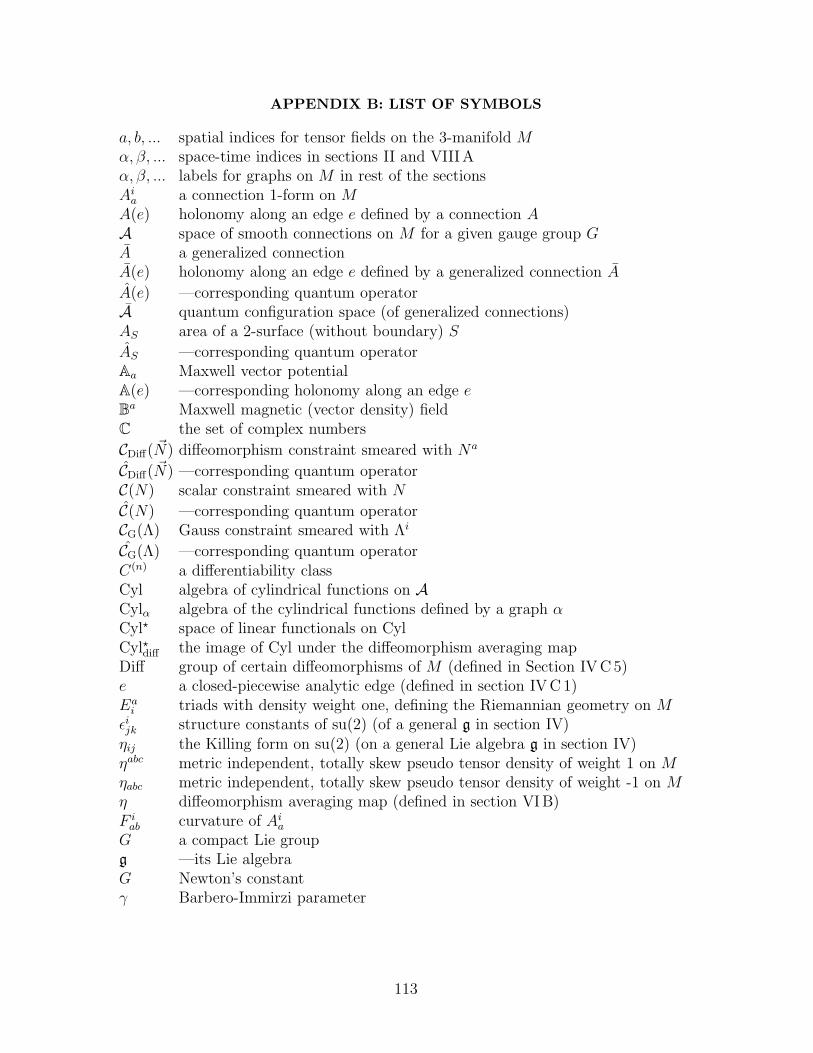
APPENDIX B: LIST OF SYMBOLS

a, b, ... spatial indices for tensor fields on the 3-manifold Mα, β, ... space-time indices in sections II and VIIIAα, β, ... labels for graphs on M in rest of the sectionsAi

a a connection 1-form on MA(e) holonomy along an edge e defined by a connection AA space of smooth connections on M for a given gauge group GA a generalized connectionA(e) holonomy along an edge e defined by a generalized connection A

A(e) —corresponding quantum operatorA quantum configuration space (of generalized connections)AS area of a 2-surface (without boundary) S

AS —corresponding quantum operatorAa Maxwell vector potentialA(e) —corresponding holonomy along an edge eBa Maxwell magnetic (vector density) fieldC the set of complex numbers

CDiff( ~N) diffeomorphism constraint smeared with Na

CDiff( ~N) —corresponding quantum operatorC(N) scalar constraint smeared with N

C(N) —corresponding quantum operatorCG(Λ) Gauss constraint smeared with Λi

CG(Λ) —corresponding quantum operatorC(n) a differentiability classCyl algebra of cylindrical functions on ACylα algebra of the cylindrical functions defined by a graph αCyl⋆ space of linear functionals on CylCyl⋆diff the image of Cyl under the diffeomorphism averaging mapDiff group of certain diffeomorphisms of M (defined in Section IVC5)e a closed-piecewise analytic edge (defined in section IVC1)Ea

i triads with density weight one, defining the Riemannian geometry on Mǫijk structure constants of su(2) (of a general g in section IV)ηij the Killing form on su(2) (on a general Lie algebra g in section IV)ηabc metric independent, totally skew pseudo tensor density of weight 1 on Mηabc metric independent, totally skew pseudo tensor density of weight -1 on Mη diffeomorphism averaging map (defined in section VIB)F i

ab curvature of Aia

G a compact Lie groupg —its Lie algebraG Newton’s constantγ Barbero-Immirzi parameter

113

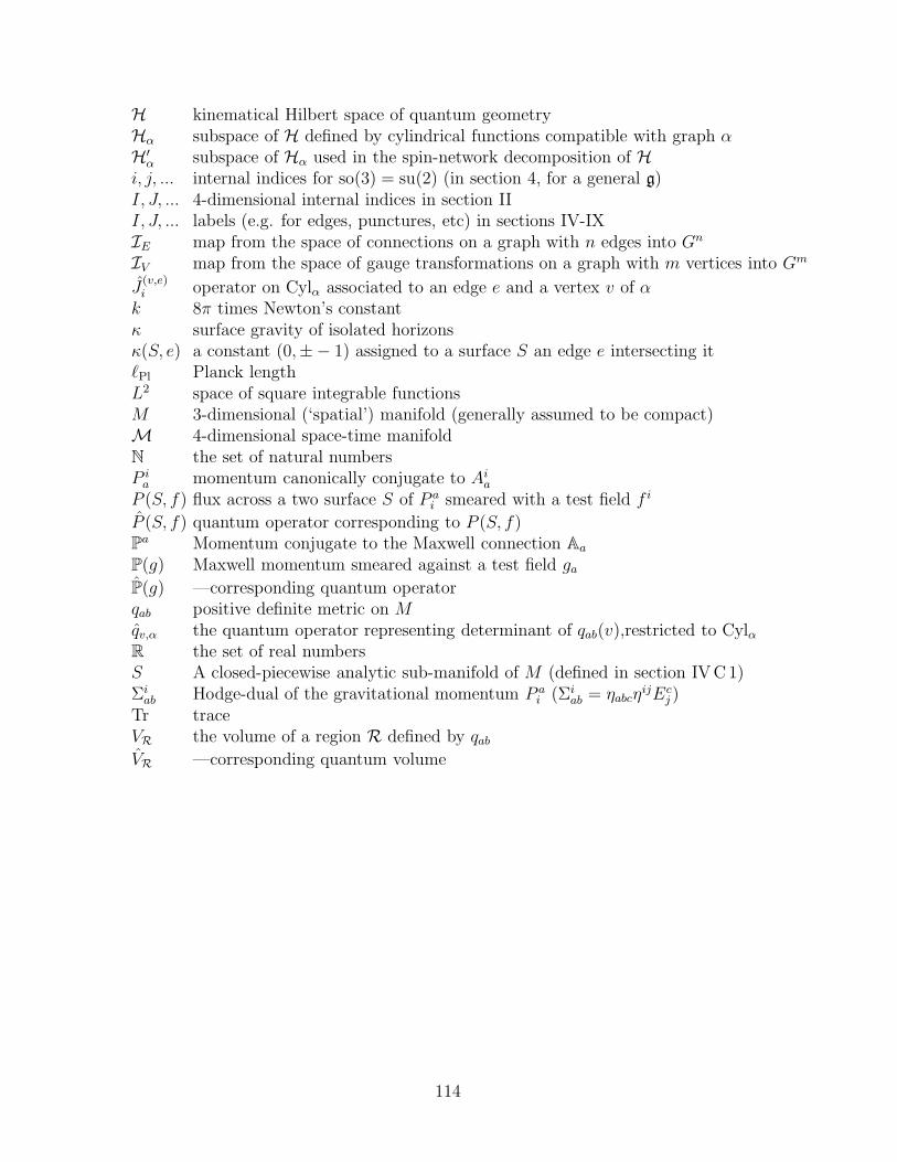
H kinematical Hilbert space of quantum geometryHα subspace of H defined by cylindrical functions compatible with graph αH′

α subspace of Hα used in the spin-network decomposition of Hi, j, ... internal indices for so(3) = su(2) (in section 4, for a general g)I, J, ... 4-dimensional internal indices in section III, J, ... labels (e.g. for edges, punctures, etc) in sections IV-IXIE map from the space of connections on a graph with n edges into Gn

IV map from the space of gauge transformations on a graph with m vertices into Gm

J(v,e)i operator on Cylα associated to an edge e and a vertex v of αk 8π times Newton’s constantκ surface gravity of isolated horizonsκ(S, e) a constant (0,±− 1) assigned to a surface S an edge e intersecting itℓPl Planck lengthL2 space of square integrable functionsM 3-dimensional (‘spatial’) manifold (generally assumed to be compact)M 4-dimensional space-time manifoldN the set of natural numbersP i

a momentum canonically conjugate to Aia

P (S, f) flux across a two surface S of P ai smeared with a test field f i

P (S, f) quantum operator corresponding to P (S, f)Pa Momentum conjugate to the Maxwell connection Aa

P(g) Maxwell momentum smeared against a test field ga

P(g) —corresponding quantum operatorqab positive definite metric on Mqv,α the quantum operator representing determinant of qab(v),restricted to CylαR the set of real numbersS A closed-piecewise analytic sub-manifold of M (defined in section IVC1)Σi

ab Hodge-dual of the gravitational momentum P ai (Σi

ab = ηabcηijEc

j )Tr traceVR the volume of a region R defined by qab

VR —corresponding quantum volume

114

REFERENCES

Books and recent reviews:

[1] Creutz M 1983 Quarks, gluons and lattices (Cambridge UP, Cambridge)[2] Ashtekar A 1991 Lectures on non-perturbative canonical gravity Notes prepared in

collaboration with R. S. Tate (World Scientific, Singapore)[3] Baez J and Muniain J P 1994 Gauge fields, knots and gravity (World Scientific, Sin-

gapore)[4] Gambini R and Pullin J 1996 Loops, knots, gauge theories and quantum gravity (Cam-

bridge UP, Cambridge)[5] Carlip S 1998 Quantum gravity in 2+1 dimensions (Cambrige UP, Cambridge)[6] Rovelli C 1998 Loop quantum gravity Living Rev. Rel 1 1[7] Bojowald M. 2001 Quantum Geometry and Symmetry (Saker-Verlag, Aachen)[8] Ashtekar A 2002 Quantum geometry and gravity: Recent Advances General Relativ-

ity and Gravitation ed Bishop N T and Maharaj S D (World Scientific, Singalore),gr-qc/0112038

[9] Thiemann T 2002 Lectures on loop quantum gravity, to appear in Aspects of quantumgravity: From theory to experimental search Lecture Notes in Physics (Springer-Verlag,Berlin 2003), gr-qc/02100942004 Modern canonical quantum general relativity, (Cambridge University Press, Cam-bridge, in press), gr-qc/0110034

[10] Perez A 2003 Spin foam models for quantum gravity Class. Quant. Grav. 20 R43–R104[11] C. Rovelli 2004 Quantum Gravity (Cambridge University Press, Cambridge, in press)

Classical theory:

[12] Ashtekar A 1986 New variables for classical and quantum gravity Phys. Rev. Lett. 57

2244–2247[13] Ashtekar A (1987) New Hamiltonian formulation of general relativity Phys. Rev. D36

1587–1602[14] Samuel J 1987 A Lagrangian basis for Ashtekar’s reformulation of canonical gravity

Pramana-J. Phys. 24 28 L429-L432Jacobson T and Smolin L 1987 The left handed spin connection as a variable forcanonical greavity Phys. Lett. B196 39-42

[15] Ashtekar A, Mazur P and Torre C G 1987 BRST structure of general relativity interms of new variables Phys. Rev D36 2955-2962

[16] Ashtekar A, Romano J D and Tate R S 1989 New variables for gravity: Inclusion ofmatter Phys. Rev. D40 2572–2587

[17] Jacobson T 1988 New variables for canonical supergravity, Class. Quant. Grav. 5 923–935Matschull H J and Nicolai H 1994 Canonical Quantum Supergravity in three-dimensions Nucl. Phys. B411 609–646

[18] Ashtekar A, Balachandran A P and Jo S 1989 The CP problem in quantum gravity,Int. J. Mod. Phys. A4 1493—1514

[19] Plebanski J F 1977 On the separation of Einsteinian substructures J. Math. Phys. 18

2511

115

[20] Capovilla R, Dell J and Jacobson T 1989 General relativity without a metric Phys.Rev. Lett. 63 2325–2328Capovilla R, Dell J, Jacobson T and Mason L 1991 Selfdual two forms and gravityClass. Quant. Grav. 8 41–57

[21] Holst S 1996 Barbero’s Hamiltonian derived from a generalized Hilbert-Palatini actionPhys. Rev. D53 5966-5969Wisniewski J 2001 Symplectic structure from Holst action, pre-print

[22] Samuel J 2000 Is Barbero’s Hamiltonian formulation a gauge theory of Lorentziangravity? Class. Quant. Grav. 17 L141-L148

[23] Robinson D C 1995 A Lagrangian formalism for the Einstein-Yang-Mills equations J.Math. Phys. 36 3733-42Lewandowski J, Okol’ow A 2000 2-Form Gravity of the Lorentzian Signature Class.Quant. Grav. 17 L47-L51

[24] Alexandrov S, Livine E R 2003 SU(2) Loop Quantum Gravity seen from CovariantTheory Phys. Rev. D67 044009

[25] Freidel L and Krasnov K 1999 BF description of higher dimensional gravity theoriesAdv. Theor. Math. Phys. 3 1289–1324

[26] Jacobson T, Romano J D 1992 Degenerate Extensions Of General Relativity Class.Quant. Grav. 9 L119–L124

[27] Matschull H J 1996 Causal structure and diffeomorphisms in Ashtekar’s gravity Class.Quant. Grav. 13 765–782

[28] Jacobson T 1996 (1+1) sector of (3+1) gravity Class. Quant. Grav. 13 L111–L116,Erratum-ibid. 1996 Class. Quant. Grav. 13 3269

[29] Lewandowski J and Wisniewski J 1997 (2+1) sector of (3+1) gravity Class. Quant.Grav. 14 775–782

[30] Lewandowski J and Wisniewski J 1999 Degenerate sectors of the Ashtekar gravityClass. Quant. Grav. 16 3057–3069

[31] Penrose R 1976 Non-linear graviton and curved twistor theory Gen. Rel.& Grav. 7

31-52[32] Ko M, Ludvigsen M, Newman E T and Tod P 1981 The theory of H space Phys. Rep.

71 51–139

Connections and loops:

[33] Rovelli C and Smolin L 1988 Knot theory and quantum gravity Phys. Rev. Lett. 61

1155-1158[34] Rovelli C and Smolin L 1990 Loop representation for quantum general relativity Nucl.

Phys. B331 80–152[35] Ashtekar A, Husain V, Rovelli C, Samuel J, and Smolin L 1989 2+1 quantum gravity

as a toy model for the 3+1 theory Class. Quant. Grav. 6 L185–L193[36] Ashtekar A, Rovelli C, and Smolin L 1991 Gravitons and loops Phys. Rev. D44 1740–

1755[37] Smolin L 1992 Recent developments in non-perturbative quantum gravity Quantum

Gravity and Csomology ed Mercader J, Sola J and Verdaguer R (World Scientific,Singapore)

[38] Goldberg J N, Lewandowski J, Stornaiolo C 1992 Degeneracy in loop variables Com-

116

mun. Math. Phys. 148 377–402

Background independent quantization of theories of connections:

[39] Ashtekar A and Isham C J 1992 Representation of the holonomy algebras of gravityand non-Abelian gauge theories Class. Quant. Grav. 9 1433–1467

[40] Ashtekar A and Lewandowski J 1994 Representation theory of analytic holonomy al-gebras, in Knots and Quantum Gravity ed Baez J C (Oxford U. Press, Oxford)

[41] Baez J C 1994 Generalized measures in gauge theory Lett. Math. Phys. 31 213–223[42] Lewandowski J 1994 Topological Measure and Graph-Differential Geometry on the

Quotient Space of Connections Int. J. Mod. Phys. D3 207–210[43] Ashtekar A, Lewandowski L, Marolf D, Mourao J and Thiemann T 1995 A manifestly

gauge invariant approach to quantum gauge theories, in Geometry of Constrained Dy-namical Systems ed Charap J M (Cambridge U. Press, Cambridge)60–72

[44] Marolf D and Mourao J 1995 On the support of the Ashtekar-Lewandowski measureCommun. Math. Phys. 170 583-606

[45] Ashtekar A and Lewandowski J 1995 Projective techniques and functional integrationJour. Math. Phys. 36 2170–2191

[46] Ashtekar A, Lewandowski L, Marolf D, Mourao J and Thiemann T 1996 CoherentState Transforms for Spaces of Connections Jour. Funct. Analysis 135 519-551

[47] Baez J C and Sawin S 1997 Functional integration on spaces of connections Jour.Funct. Analysis 150 1–27

[48] Ashtekar A, Corichi A and Zapata J A 1998 Quantum theory of geometry: III. Non-commutativity of Riemannian structures Class. Quant. Grav. 15 2955–2972

[49] Marolf D, Mourao J, Thiemann T 1997 The Status of Diffeomorphism Superselectionin Euclidean 2+1 Gravity J. Math. Phys. 38 4730-4740

[50] Mourao J M, Thiemann T, Velhinho J M 1999 Physical Properties of Quantum FieldTheory Measures J. Math. Phys. 40 2337–2353

[51] Velhinho J M 2002 A groupoid approach to spaces of generalized connections J. Geom.Phys. 41 166–180

[52] Fleischhack C 2000 Stratification of the Generalized Gauge Orbit Space Commun.Math. Phys. 214 607–649

[53] Fleischhack C 2003 On the Gribov Problem for Generalized Connections Commun.Math. Phys. 234 423–454

[54] Fleischhack C 2003 Hyphs and the Ashtekar-Lewandowski Measure J. Geom. Phys. 45

231–251[55] Sahlmann H 2002 When Do Measures on the Space of Connections Support the Triad

Operators of Loop Quantum Gravity? Preprint gr-qc/0207112Sahlmann H 2002 Some Comments on the Representation Theory of the Algebra Un-derlying Loop Quantum Gravity Preprint gr-qc/0207111

[56] Okolow A, Lewandowski J 2003 Diffeomorphism covariant representations of theholonomy-flux star-algebra Class. Quant. Grav. 20 3543–3568

[57] Sahlmann H and Thiemann T 2003 On the superselection theory of the Weyl algebrafor diffeomorphism invariant quantum gauge theories Preprint gr-qc/0302090Sahlmann H and Thiemann T 2003 Irreducibility of the Ashtekar-Isham-Lewandowskirepresentation Preprint gr-qc/0303074

117

[58] Lewandowski J, Okolow A, Sahlmann H, Thiemann T 2003 Uniqueness of the diffeo-morphism invariant state on the quantum holonomy-flux algebra Preprint

Spin networks:

[59] Penrose R 1971 Angular momentum: an approach to combinatorial space-time Quan-tum Theory and Beyond ed Bastin T (Cambridge University Press)

[60] Rovelli C and Smolin L 1995 Spin networks and quantum gravity Phys. Rev. D52

5743–5759[61] Baez J C 1996 Spin networks in non-perturbative quantum gravity, in The Interface

of Knots and Physics ed Kauffman L (American Mathematical Society, Providence)pp. 167–203Baez J C 1996 Spin networks in gauge theory Adv. Math.117 253–272

[62] Thiemann T 1998 The inverse loop transform J. Math. Phys. 39 1236–1248[63] Baez J C and Sawin S 1998 Diffeomorphism–invariant spin network states Jour. Funct.

Analysis 158 253–266[64] C Fleischhack 2003 Proof of a Conjecture by Lewandowski and Thiemann Preprint

math-ph/0304002

Geometric operators and their properties

[65] Rovelli C and Smolin L 1995 Discreteness of area and volume in quantum gravity Nucl.Phys. B442 593–622; Erratum: Nucl. Phys. B456 753

[66] Ashtekar A and Lewandowski L 1995 Differential geometry on the space of connectionsusing projective techniques Jour. Geo. & Phys. 17 191–230

[67] Loll R 1995 The volume operator in discretized quantum gravity Phys. Rev. Lett. 75

3048–3051[68] Loll R 1995 Spectrum of the Volume Operator in Quantum Gravity Nucl. Phys. B460

143–154[69] Frittelli S, Lehner L and Rovelli C 1996 Class. Quant. Grav. 13 2921–2932[70] De Pietri R, Rovelli C 1996 Phys. Rev. D54 2664–2690[71] Lewandowski J. 1997 Volume and Quantizations Class. Quant. Grav. 14 71–76[72] Ashtekar A and Lewandowski J 1997 Quantum theory of geometry I: Area operators

Class. Quant. Grav. 14 A55–A81[73] Ashtekar A and Lewandowski J 1997 Quantum theory of geometry II: Volume Opera-

tors Adv. Theo. Math. Phys. 1 388–429[74] Loll R 1997 Simplifying the spectral analysis of the volume operator Nucl. Phys. B500

405–420[75] Loll R 1997 Further results on geometric operators in quantum gravity Class. Quant.

Grav. 14 1725–1741[76] De Pietri R 1997 Spin Networks and Recoupling in Loop Quantum Gravity Nucl. Phys.

Suppl 57 251-254[77] De Pietri R 1997 On the relation between the connection and the loop representation

of quantum gravity Class. Quant. Grav. 14 53–70[78] Thiemann T 1998 Closed formula for the matrix elements of the volume operator in

canonical quantum gravity J. Math. Phys. 39 3347-3371[79] Thiemann T 1998 A length operator for canonical quantum gravity Jour. Math. Phys.

118

39 3372–3392[80] Major S A 1999 Operators for quantized directions Class. Quant. Grav. 16 3859-3877

Barbero-Immirzi ambiguity

[81] Barbero F 1996 Real Ashtekar variables for Lorentzian signature space-times Phys.Rev. D51 5507–5510

[82] Immirzi G 1997 Quantum gravity and Regge calculus Nucl. Phys. Proc. Suppl. 57

65–72[83] Rovelli C. and Thiemann T. (1998) The Immirizi parameter in quantum general rela-

tivity Phys. Rev. D57 1009–1014[84] Gambini R, Obregon O and Pullin J 1999 Yang-Mills analogs of the Immirzi ambiguity

Phys. Rev. D59 047505

Quantum Einstein’s equation I

[85] Kuchar K 1993 Canonical Quantum Gravity General Relativity and Gravitation 1992ed Gleiser R J, Kozameh C N, Moreschi O M (Institute of Physics Publishing) 119–150

[86] Ashtekar A, Tate R S and Uggla C 1993 Minisuperspaces: Observables and quantiza-tion Int. J. Phys. D2 15–50Ashtekar A, Tate R S and Uggla C 1993 Minisuperspaces: Symmetries and quantiza-tion Misner Festschrift ed Hu B L et al (Cambridge U. P., Cambridge)

[87] Ashtekar A and Tate R S 1994 An algebraic extension of Dirac quantization: ExamplesJour. Math. Phys. 35 6434–6470

[88] Marolf D 1995 Refined algebraic quantization: Systems with a single constraintPreprint gr-qc/9508015

[89] Ashtekar A, Lewandowski J, Marolf D, Mourao J and Thiemann T 1995 Quantizationof diffeomorphism invariant theories of connections with local degrees of freedom Jour.Math. Phys. 36 6456–6493

[90] Marolf D, Mourao J and Thiemann T 1997 The status of diffeomorphism super-selection in Euclidean 2+1 gravity J. Math. Phys. 38 4730-4740

[91] Guilini N and Marolf D 1999 On the Generality of Refined Algebraic QuantizationClass. Quant. Grav.16 2479–2488A uniqueness theorem for constraint quantization Class. Quant. Grav. 16 2489–2505

[92] Lewandowski J and Thiemann T 1999 Diffeomorphism invariant quantum field theoriesof connections in terms of webs Class. Quant. Grav. 16 2299–2322

[93] Corichi A and Zapata J A 1997 On diffeomorphism invariance for lattice theories Nucl.Phys. B493 475–490

Quantum Einstein’s equation II

[94] Rovelli C and Smolin L 1994 The physical Hamiltonian in nonperturbative quantumgravity Phys. Rev. Lett. 72 446–449

[95] Thiemann T 1996 Anomaly-free formulation of non-perturbative, four-dimensionalLorentzian quantum gravity Phys. Lett. B380 257–264

[96] Thiemann T 1998 Quantum spin dynamics (QSD) Class. Quant. Grav. 15 839–873[97] Thiemann T. 1998 QSD III: Quantum constraint algebra and physical scalar product

in quantum general relativity Class. Quant. Grav. 15 1207–1247

119

[98] Thiemann T 1998 QSD V: Quantum gravity as the natural regulator of matter quantumfield theories Class. Quant. Grav. 15 1281–1314

[99] Thiemann T 2001 Quantum Spin Dynamics (QSD) : VII. Symplectic Structures andContinuum Lattice Formulations of Gauge Field Theories Class. Quant. Grav. 18 3293–3338

[100] Gambini R, Lewandowski J, Marolf D and Pullin J 1998 On the consistency of theconstraint algebra in spin network quantum gravity Int. J. Mod. Phys. D7 97–109

[101] Lewandowski J and Marolf D 1998 Loop constraints: A habitat and their algebra Int.J. Mod. Phys. D7 299–330

[102] Gaul G and Rovelli C 2001 Generalized hamiltonian constraint operator in loop quan-tum gravity and its simplest Euclidean matrix elements Class. Quant. Grav. 18 1593–1624

Big-bang:

[103] Kodama H 1988 Specialization of Ashtekar’s formalism to Bianchi cosmology Prog.Theor. Phys. 80 1024–1040Kodama H 1990 Holomorphic wavefunction of the universe Phys. Rev. D42 2548–2565

[104] Bojowald M 2001 Absence of singularity in loop quantum cosmology Phys. Rev. Lett.86 5227–5230

[105] Bojowald M 2001 Inverse scale factor in isotropic quantum geometry Phys. Rev. D64

084018[106] Bojowald M 2001 Dynamical initial conditions in quantum cosmology Phys. Rev. Lett.

87 121301[107] Bojowald M 2001 Loop Quantum Cosmology IV: Discrete Time Evolution Class.

Quant. Grav. 18 1071–1088[108] Bojowald M 2001 Loop quantum cosmology III: Wheeler-DeWitt operators Class.

Quant. Grav. 18 1055–1070Bojowald M 2002 The Semiclassical Limit of Loop Quantum Cosmology Class. Quant.Grav. 18 L109–L116

[109] Bojowald M 2001 The Inverse Scale Factor in Isotropic Quantum Geometry Phys.Rev.D64 084018

[110] Bojowald M 2002 Isotropic Loop Quantum Cosmology Class.Quant.Grav. 19 2717–2742

[111] Bojowald M, Hinterleitner F 2002 Isotropic Loop Quantum Cosmology with MatterPhys.Rev. D66 104003

[112] Bojowald M and Vandersloot K 2003 Loop Quantum Cosmology, Boundary Proposals,and Inflation Phys.Rev. D67 124023

[113] Bojowald M 2003 Homogeneous Loop Quantum Cosmology Class.Quant.Grav. 20

2595–2615[114] Bojowald M 2003 Initial Conditions for a Universe Gen. Rel. Grav. 35, 1877-1883

(First Prize in the Gravity Research Foundation Essay Contest)[115] Ashtekar A, Bojowald M, Lewandowski J 2003 Mathematical structure of loop quantum

cosmology Adv. Theor. Math. Phys. 7 233–268[116] Bojowald M, Date G and Vandersloot K 2004 Homogeneous Loop Quantum Cosmol-

ogy: The Role of the Spin Connection Class. Quant. Grav. textbf21 1253-1278

120

[117] Ashtekar A, Bojowald M and Willis J 2004 Quantum corrections to Friedmann equa-tions in loop quantum cosmology (in preparation)

Black holes:

[118] Bekenstein J D 1973 Black holes and entropy Phys. Rev. D7 2333–2346(1974) Generalized second law of thermodynamics in black hole physics Phys. Rev. D9

3292–3300Bekenstein J D and Meisels A 1977 Einstein A and B coefficients for a black hole Phys.Rev. D15 2775–2781

[119] Bardeen J W, Carter B and Hawking S W 1973 The four laws of black hole mechanicsCommun. Math. Phys. 31 161-170

[120] Hawking S W 1975 Particle creation by black holes Commun. Math. Phys. 43 199–220[121] Gibbons G and Hawking S W 1977 Cosmological event horizons, thermodynamics, and

particle creation Phys. Rev.D15 2738–2751[122] Smolin L 1995 Linking topological quantum field theory and nonperturbative quantum

gravity J. Math. Phys. 36 6417–6455[123] Barreira M, Carfora M and Rovelli C 1996 Physics with non-perturbative quantum

gravity: radiation from a quantum black hole Gen. Rel. Grav. 28 1293–1299Rovelli C 1996 Black hole entropy from loop quantum gravity Phys. Rev. Lett. 14

3288–3291Rovelli C 1996 Loop quantum gravity and black hole physics Helv. Phys. Acta. 69

582–611[124] Krasnov K 1997 Geometrical entropy from loop quantum gravity Phys. Rev. D55

3505–3513Krasnov K 1998 On statistical mechanics of Schwarzschild black holes Gen. Rel. Grav.30 53–68

[125] Jacobson T, Kang G and Myers R C 1994 On black hole entropy Phys. Rev. D496587–6598

[126] Wald R. (1993) Black hole entropy is Noether charge Phys. Rev. D48 3427–3431Iyer V and Wald R 1994 Some properties of Noether charge and a proposal for dynam-ical black hole entropy Phys. Rev. D50 846–864

[127] Ashtekar A, Baez J C, Corichi A, and Krasnov K 1998 Quantum geometry and blackhole entropy (1998) Phys. Rev. Lett. 80 904–907

[128] Ashtekar A, Corichi A and Krasnov K 1999 Isolated horizons: the classical phase spaceAdv. Theor. Math. Phys. 3 418–471

[129] Ashtekar A, Baez J C and Krasnov K 2000 Quantum geometry of isolated horizonsand black hole entropy Adv. Theo. Math. Phys. 4 1–95

[130] Kaul R K and Majumdar P 2000 Logarithmic corrections to the Bekenstein-Hawkingentropy Phys. Rev. Lett. 84 5255–5257

[131] Ashtekar A, Beetle C and Fairhurst S 1999 Isolated horizons: a generalization of blackhole mechanics Class. Quantum Grav. 16 L1–L7Ashtekar A, Beetle C and Fairhurst S 2000 Mechanics of isolated horizons Class. Quan-tum Grav. 17 253–298

[132] Lewandowski J 2000 Space-times admitting isolated horizons Class. Quantum Grav.17 L53–L59

121

[133] Ashtekar A, Fairhurst S and Krishnan B 2000 Isolated Horizons: Hamiltonian Evolu-tion and the First Law Phys. Rev. D62 104025.

[134] Ashtekar A, Beetle C and Lewandowski J 2001 Mechanics of rotating isolated horizonsPhy. Rev. D64 044016

[135] Ashtekar A, Beetle C and Lewandowski J 2002 Geometry of generic isolated horizonsClass. Quantum Grav. 19 1195–1225

[136] Ashtekar A, Corichi A and Sudarski D 2003 Non-Minimally Coupled Scalar Fields andIsolated Horizons Class. Quantum Grav. 20 3413-3425

[137] Ashtekar A and Corichi A 2003 Non-minimal couplings, quantum geometry and blackhole entropy 20 Class. Quantum Grav. 20 4473-4484

[138] Ashtekar A, Engle J, Pawlowski, T and van der Broeck C 2004 Multipole moments ofisolated horizons Class. Quant. Grav. 21 2549-2570

[139] Ashtekar A 2003 Black hole entropy: Inclusion of distortion and angular momentum,http://www.phys.psu.edu/events/index.html?event id=517&event type=17Ashtekar A, Engle J and van der Broeck C 2004 (in preparation)

[140] Wheeler J A 1992 It from bit Sakharov Memorial Lectures on Physics, Vol 2 ed KeldyshL and Feinberg V (Nova Science, Moscow)

[141] Ghosh A and Mitra P 2004 A bound on the log correction to the black hole area lawpre-print gr-qc/0401070

Low energy physics:

[142] Ashtekar A, Rovelli C and Smolin L 1992 Weaving a classical geometry with quantumthreads Phy. Rev. Lett. 69 237–240

[143] Arnsdorf M, Gupta S 2000 Loop quantum gravity on non-compact spaces Nucl. Phys.B577 529-546

[144] Corichi A, Reyes J M 2001 A Gaussian Weave for Kinematical Loop Quantum GravityInt. J. Mod. Phys. D10 325-338

[145] Hall B C 1994 The Segal-Bergmann coherent state transform for compact Lie Liegroups J. Funct. Anal. 122 103-151

[146] Sahlmann H, Thiemann T and Winkler O 2001 Coherent states for canonical quantumgeneral relativity and the infinite tensor product extension Nucl. Phys. B606 401-440

[147] Thiemann T 2001 Gauge field theory coherent states (GCS): I. general properties Class.Quant. Grav. 18 2025-2064T. Thiemann, O. Winkler 2001 Gauge Field Theory Coherent States (GCS) : II.Peakedness Properties Class. Quant. Grav. 18 2561–2636Thiemann T, Winkler O 2001 Gauge Field Theory Coherent States (GCS) : III. Ehren-fest Theorems Class. Quant. Grav. 18 4629-4682Thiemann T, Winkler O 2001 Gauge Field Theory Coherent States (GCS) : IV. InfiniteTensor Product and Thermodynamical Limit Class. Quant. Grav. 18 4997-5054

[148] Hanno Sahlmann, Thomas Thiemann 2002 Towards the QFT on Curved SpacetimeLimit of QGR. I: A General Scheme Preprint gr-qc/0207030

Sahlmann H Thomas Thiemann 2002 Towards the QFT on Curved Spacetime Limitof QGR. II: A Concrete Implementation Preprint gr-qc/0207031

[149] Thiemann T 2002 Complexifier Coherent States for Quantum General RelativityPreprint gr-qc/0206037

122

[150] Bombelli L 2002 Statistical geometry of random weave states Proceedings of the NinthMarcel Grossmann Meeting on General Relativity ed Gurzadyan VG, Jantzen RT, andRuffini R (World Scientific, Singapore) gr-qc/0101080

[151] Ashtekar A and Isham C J 1992 Phys. Lett. B274 393-398[152] Varadarajan M 2000 Fock representations from U(1) holonomy algebras Phys. Rev.

D61 104001Varadarajan M. (2001) M. Photons from quantized electric flux representations Phys.Rev. D64 104003

[153] Ashtekar A and Lewandowski J 2001 Relation between polymer and Fock excitationsClass. Quant. Grav. 18 L117–L127

[154] Velhinho J M 2002 Invariance properties of induced Fock measures for U(1) holonomiesCommun. Math. Phys. 227 541–550

[155] Ashtekar A, Fairhurst S and Willis J 2003 Quantum gravity, shadow states, and quan-tum mechanics Class. Quantum Grav. 20, 1031-1061

[156] Ashtekar A, Fairhurst S and Ghosh A 2004 (in preparation)[157] Varadarajan M. 2002 Gravitons from a loop representation of linearised gravity Phys.

Rev. D66 024017[158] Ashtekar A, Ghosh A and Van Den Broeck C 2004 (in preparation)[159] Bobienski M, Lewandowski J, Mroczek M 2002 A 2-Surface Quantization of the

Lorentzian Gravity Proceedings of the Ninth Marcel Grossmann Meeting on GeneralRelativity ed Gurzadyan VG, Jantzen RT, and Ruffini R (World Scientific, Singapore)gr-qc/0101069

[160] Ashtekar A, Lewandowski J and Sahlmann H 2003 Polymer and Fock representationsof a scalar field Class. Quant. Grav. 20 L11–L21

Spin foams and finiteness:

[161] Baez J C 2000 An introduction to spin foam models of quantum gravity and BF theoryLect. Notes Phys. 543 25–94

[162] Baez J C 1998 Spin foam models Class. Quant. Grav. 15 1827–1858[163] Reisenberger M P 1997 A lattice worldsheet sum for Reisenberger M P 1997 4-d Eu-

clidean general relativity Preprint gr-qc/9711052Reisenberger M P 1999 On relativistic spin network vertices J. Math. Phys. 40 2046–2054

[164] Reisenberger M P and Rovelli C 2001 Spacetime as a Feynman diagram: the connectionformulation Class. Quant. Grav. 18 121–140Reisenberger M P and Rovelli 2002 Spacetime states and covariant quantum theoryPhys. Rev. D65 125016

[165] Barrett J W and Crane L 1998 Relativistic spin networks and quantum gravity J.Math. Phys. 39 3296–3302Barrett J W and Crane L 2000 A Lorentzian signature model for quantum generalrelativity Class. Quant. Grav. 17 3101–3118

[166] Perez A 2001 Finiteness of a spinfoam model for Euclidean quantum general relativityNucl. Phys. B599 427–434Perez A and Rovelli C 2001 Spin foam model for Lorentzian general relativity Phys.Rev. D63 041501

123

Crane L, Perez A and Rovelli C 2001 Perturbative finiteness in spin-foam quantumgravity Phys. Rev. Lett. 87 181301Crane L, Perez A and Rovelli C 2001 3+1 spinfoam model of quantum gravity withspacelike and timelike components Phys. Rev. D64 064002

[167] Baez J, Christensen D, Halford T R, Tsang DC 2002 Spin Foam Models of RiemannianQuantum Gravity Class. Quant. Grav. 194627-4648

[168] Gambini R and Pullin J 2002 A finite spin-foam-based theory of three and four dimen-sional quantum gravity Phys. Rev. D66 024020

[169] Lauscher O and Reuter M 2002 Is quantum Einstein gravity non-perturbatively renor-malizable? Class. Quant. Grav. 19 483–492

[170] Percacci R and Perini D 2003 Asymptotic safety of gravity coupled to matter Phys.Rev. D68044018Perini D 2003 Gravity and matter with asymptotic safety pre-print hep-th/0305053

[171] Bojowald M and Perez A 2003 Spin foam quantization and anomalies gr-qc/0303026[172] Freidel L and Louapre D 2003 Diffeomorphisms and spin foam models, Nucl.Phys.

B662 279-298Freidel L and Louapre D 2003 Non-perturbative summation over 3D discrete topologiesPhys. Rev. D68 104004 hep-th/0211026

[173] Perez A and Noui K 2004 Three dimensional loop quantum gravity: coupling to pointparticles pre-print gr-qc/0402111

2004 Three dimensional loop quantum gravity: physical scalar product and spin foammodels pre-print gr-qc/0402110

Outlook:

[174] Ashtekar A, Lewandowski J, Marolf D, Mourao J and Thiemann T 1997 SU(N) Quan-tum Yang-Mills theory in two dimensions: A complete solution J. Math. Phys. 38,5453-5482

[175] Ashtekar A and Sahlmann H 2004 (in preparation)[176] Okolw A 204 Representations of quantum geometry Ph.D. thesis, University of Warsaw[177] Rovelli C and Speziale S 2003 Reconcile Planck-scale discreteness and the Lorentz-

Fitzgerald contraction Phys. Rev. D67 064019[178] Thiemann T 2003 The Phoenix project: Master constraint programme for loop quan-

tum gravity Preprint gr-qc/0305080[179] Dittrich B 2004 Testing the master constraint programme for loop quantum gravity

http://www.phys.psu.edu/events/index.html?event id=850&event type=17[180] Klauder J 2003 Affine quantum gravity Int. J. Mod. Phys. D12 1769-1774

2004 The utility of coherent states and other mathematical methods in the foundationsof affine quantum gravity, pre-print hep-th/0401214

[181] Di Bartolo C, Gambini R, Griego J and Pullin J 2000 Consistent canonical quantiza-tion of general relativity in the space of Vassiliev knot invariants Phys. Rev. Lett. 84

2314–23172000 Canonical quantum gravity in the Vassiliev invariants arena: I. Kinematical struc-ture Class. Quant. Grav. 17 3211-32382000 Canonical quantum gravity in the Vassiliev invariants arena: II. Constraints,habitats and consistency of the constraint algebra Class. Quant. Grav. 17 3239-3264

124

[182] Gambini R and Pullin J 2003 Canonical quantization of general relativity in discretespace-times Phys. Rev. Lett. 90 021301Gambini R, Porto R and Pullin J 2004 Loss of coherence from discrete quantum gravityClass. Quant. Grav. 21 L51-L57Gambini R, Porto R and Pullin J 2004 A relational solution to the problem of timein quantum mechanics and quantum gravity induces a fundamental mechanism forquantum decoherence pre-print gr-qc/0402118

[183] Horowitz G. T. 1998 Quantum states of black holes, in Black Holes and RelativisticStars, ed Wald R M ( University of Chicago Press, Chicago)

[184] Carlip S 1999 Entropy from Conformal Field Theory at Killing Horizons Class. Quant.Grav. 16 3327–3348

[185] Dreyer O, Ghosh A and Wisniewski J 2001 Black hole entropy calculations based onsymmetries, Class. Quant. Grav.18 1929-1938

[186] Carlip S 2002 Near-Horizon Conformal Symmetry and Black Hole Entropy Phys. Rev.Lett. 88 241301

[187] Ashtekar A, Krishnan B 2002 Dynamical Horizons: Energy, Angular Momentum,Fluxes and Balance Laws, Phys. Rev. Lett. 89 2611012003 Dynamical horizons and their properties, Phys. Rev. D68 104030

[188] Bojowald M 2002 Inflation from Quantum Geometry Phys.Rev.Lett. 89 261301[189] Bojowald M and Date G 2004 Quantum suppression of the generic chaotic behavior

close to cosmological singularities Phys. Rev. Lett. 92 071302[190] Tsujikawa S, Singh P and Maartens R 2003 Loop quantum gravity effects on inflation

and the CMB, pre-print astro-ph/0311015

125