arX

iv:h

ep-e

x/01

0601

2v3

29

Sep

2001

Searches for New Physics in Events with a Photon and b–quark Jet at CDF(May 14, 2007)

T. Affolder,23 H. Akimoto,45 A. Akopian,37 M. G. Albrow,11 P. Amaral,8 D. Amidei,25 K. Anikeev,24 J. Antos,1

G. Apollinari,11 T. Arisawa,45 A. Artikov,9 T. Asakawa,43 W. Ashmanskas,8 F. Azfar,30 P. Azzi-Bacchetta,31

N. Bacchetta,31 H. Bachacou,23 S. Bailey,16 P. de Barbaro,36 A. Barbaro-Galtieri,23 V. E. Barnes,35 B. A. Barnett,19

S. Baroiant,5 M. Barone,13 G. Bauer,24 F. Bedeschi,33 S. Belforte,42 W. H. Bell,15 G. Bellettini,33 J. Bellinger,46

D. Benjamin,10 J. Bensinger,4 A. Beretvas,11 J. P. Berge,11 J. Berryhill,8 A. Bhatti,37 M. Binkley,11 D. Bisello,31

M. Bishai,11 R. E. Blair,2 C. Blocker,4 K. Bloom,25 B. Blumenfeld,19 S. R. Blusk,36 A. Bocci,37 A. Bodek,36

W. Bokhari,32 G. Bolla,35 Y. Bonushkin,6 D. Bortoletto,35 J. Boudreau,34 A. Brandl,27 S. van den Brink,19

C. Bromberg,26 M. Brozovic,10 E. Brubaker,23 N. Bruner,27 E. Buckley-Geer,11 J. Budagov,9 H. S. Budd,36

K. Burkett,16 G. Busetto,31 A. Byon-Wagner,11 K. L. Byrum,2 S. Cabrera,10 P. Calafiura,23 M. Campbell,25

W. Carithers,23 J. Carlson,25 D. Carlsmith,46 W. Caskey,5 A. Castro,3 D. Cauz,42 A. Cerri,33 A. W. Chan,1

P. S. Chang,1 P. T. Chang,1 J. Chapman,25 C. Chen,32 Y. C. Chen,1 M. -T. Cheng,1 M. Chertok,5 G. Chiarelli,33

I. Chirikov-Zorin,9 G. Chlachidze,9 F. Chlebana,11 L. Christofek,18 M. L. Chu,1 Y. S. Chung,36 C. I. Ciobanu,28

A. G. Clark,14 A. Connolly,23 J. Conway,38 M. Cordelli,13 J. Cranshaw,40 R. Cropp,41 R. Culbertson,11

D. Dagenhart,44 S. D’Auria,15 F. DeJongh,11 S. Dell’Agnello,13 M. Dell’Orso,33 L. Demortier,37 M. Deninno,3

P. F. Derwent,11 T. Devlin,38 J. R. Dittmann,11 A. Dominguez,23 S. Donati,33 J. Done,39 M. D’Onofrio,33 T. Dorigo,16

N. Eddy,18 K. Einsweiler,23 J. E. Elias,11 E. Engels, Jr.,34 R. Erbacher,11 D. Errede,18 S. Errede,18 Q. Fan,36

R. G. Feild,47 J. P. Fernandez,11 C. Ferretti,33 R. D. Field,12 I. Fiori,3 B. Flaugher,11 G. W. Foster,11 M. Franklin,16

J. Freeman,11 J. Friedman,24 H. J. Frisch,8 Y. Fukui,22 I. Furic,24 S. Galeotti,33 A. Gallas,(∗∗) 16 M. Gallinaro,37

T. Gao,32 M. Garcia-Sciveres,23 A. F. Garfinkel,35 P. Gatti,31 C. Gay,47 D. W. Gerdes,25 P. Giannetti,33 V. Glagolev,9

D. Glenzinski,11 M. Gold,27 J. Goldstein,11 I. Gorelov,27 A. T. Goshaw,10 Y. Gotra,34 K. Goulianos,37 C. Green,35

G. Grim,5 P. Gris,11 L. Groer,38 C. Grosso-Pilcher,8 M. Guenther,35 G. Guillian,25 J. Guimaraes da Costa,16

R. M. Haas,12 C. Haber,23 S. R. Hahn,11 C. Hall,16 T. Handa,17 R. Handler,46 W. Hao,40 F. Happacher,13

K. Hara,43 A. D. Hardman,35 R. M. Harris,11 F. Hartmann,20 K. Hatakeyama,37 J. Hauser,6 J. Heinrich,32

A. Heiss,20 M. Herndon,19 C. Hill,5 K. D. Hoffman,35 C. Holck,32 R. Hollebeek,32 L. Holloway,18 R. Hughes,28

J. Huston,26 J. Huth,16 H. Ikeda,43 J. Incandela,11 G. Introzzi,33 J. Iwai,45 Y. Iwata,17 E. James,25 M. Jones,32

U. Joshi,11 H. Kambara,14 T. Kamon,39 T. Kaneko,43 K. Karr,44 H. Kasha,47 Y. Kato,29 T. A. Keaffaber,35

K. Kelley,24 M. Kelly,25 R. D. Kennedy,11 R. Kephart,11 D. Khazins,10 T. Kikuchi,43 B. Kilminster,36 B. J. Kim,21

D. H. Kim,21 H. S. Kim,18 M. J. Kim,21 S. B. Kim,21 S. H. Kim,43 Y. K. Kim,23 M. Kirby,10 M. Kirk,4

L. Kirsch,4 S. Klimenko,12 P. Koehn,28 K. Kondo,45 J. Konigsberg,12 A. Korn,24 A. Korytov,12 E. Kovacs,2

J. Kroll,32 M. Kruse,10 S. E. Kuhlmann,2 K. Kurino,17 T. Kuwabara,43 A. T. Laasanen,35 N. Lai,8 S. Lami,37

S. Lammel,11 J. Lancaster,10 M. Lancaster,23 R. Lander,5 A. Lath,38 G. Latino,33 T. LeCompte,2 A. M. Lee IV,10

K. Lee,40 S. Leone,33 J. D. Lewis,11 M. Lindgren,6 T. M. Liss,18 J. B. Liu,36 Y. C. Liu,1 D. O. Litvintsev,11

O. Lobban,40 N. Lockyer,32 J. Loken,30 M. Loreti,31 D. Lucchesi,31 P. Lukens,11 S. Lusin,46 L. Lyons,30 J. Lys,23

R. Madrak,16 K. Maeshima,11 P. Maksimovic,16 L. Malferrari,3 M. Mangano,33 M. Mariotti,31 G. Martignon,31

A. Martin,47 J. A. J. Matthews,27 J. Mayer,41 P. Mazzanti,3 K. S. McFarland,36 P. McIntyre,39 E. McKigney,32

M. Menguzzato,31 A. Menzione,33 C. Mesropian,37 A. Meyer,11 T. Miao,11 R. Miller,26 J. S. Miller,25 H. Minato,43

S. Miscetti,13 M. Mishina,22 G. Mitselmakher,12 N. Moggi,3 E. Moore,27 R. Moore,25 Y. Morita,22 T. Moulik,35

M. Mulhearn,24 A. Mukherjee,11 T. Muller,20 A. Munar,33 P. Murat,11 S. Murgia,26 J. Nachtman,6 V. Nagaslaev,40

S. Nahn,47 H. Nakada,43 I. Nakano,17 C. Nelson,11 T. Nelson,11 C. Neu,28 D. Neuberger,20 C. Newman-Holmes,11 C.-Y. P. Ngan,24 H. Niu,4 L. Nodulman,2 A. Nomerotski,12 S. H. Oh,10 Y. D. Oh,21 T. Ohmoto,17 T. Ohsugi,17 R. Oishi,43

T. Okusawa,29 J. Olsen,46 W. Orejudos,23 C. Pagliarone,33 F. Palmonari,33 R. Paoletti,33 V. Papadimitriou,40

D. Partos,4 J. Patrick,11 G. Pauletta,42 M. Paulini,(∗) 23 C. Paus,24 L. Pescara,31 T. J. Phillips,10 G. Piacentino,33

K. T. Pitts,18 A. Pompos,35 L. Pondrom,46 G. Pope,34 M. Popovic,41 F. Prokoshin,9 J. Proudfoot,2 F. Ptohos,13

O. Pukhov,9 G. Punzi,33 A. Rakitine,24 F. Ratnikov,38 D. Reher,23 A. Reichold,30 A. Ribon,31 W. Riegler,16

F. Rimondi,3 L. Ristori,33 M. Riveline,41 W. J. Robertson,10 A. Robinson,41 T. Rodrigo,7 S. Rolli,44 L. Rosenson,24

R. Roser,11 R. Rossin,31 A. Roy,35 A. Ruiz,7 A. Safonov,12 R. St. Denis,15 W. K. Sakumoto,36 D. Saltzberg,6

C. Sanchez,28 A. Sansoni,13 L. Santi,42 H. Sato,43 P. Savard,41 P. Schlabach,11 E. E. Schmidt,11 M. P. Schmidt,47

M. Schmitt,(∗∗) 16 L. Scodellaro,31 A. Scott,6 A. Scribano,33 S. Segler,11 S. Seidel,27 Y. Seiya,43 A. Semenov,9

F. Semeria,3 T. Shah,24 M. D. Shapiro,23 P. F. Shepard,34 T. Shibayama,43 M. Shimojima,43 M. Shochet,8 A. Sidoti,31

J. Siegrist,23 A. Sill,40 P. Sinervo,41 P. Singh,18 A. J. Slaughter,47 K. Sliwa,44 C. Smith,19 F. D. Snider,11 A. Solodsky,37

J. Spalding,11 T. Speer,14 P. Sphicas,24 F. Spinella,33 M. Spiropulu,16 L. Spiegel,11 J. Steele,46 A. Stefanini,33

J. Strologas,18 F. Strumia, 14 D. Stuart,11 K. Sumorok,24 T. Suzuki,43 T. Takano,29 R. Takashima,17 K. Takikawa,43

P. Tamburello,10 M. Tanaka,43 B. Tannenbaum,6 M. Tecchio,25 R. Tesarek,11 P. K. Teng,1 K. Terashi,37 S. Tether,24

A. S. Thompson,15 R. Thurman-Keup,2 P. Tipton,36 S. Tkaczyk,11 D. Toback,39 K. Tollefson,36 A. Tollestrup,11

1

D. Tonelli,33 H. Toyoda,29 W. Trischuk,41 J. F. de Troconiz,16 J. Tseng,24 N. Turini,33 F. Ukegawa,43 T. Vaiciulis,36

J. Valls,38 S. Vejcik III,11 G. Velev,11 G. Veramendi,23 R. Vidal,11 I. Vila,7 R. Vilar,7 I. Volobouev,23 M. von der Mey,6

D. Vucinic,24 R. G. Wagner,2 R. L. Wagner,11 N. B. Wallace,38 Z. Wan,38 C. Wang,10 M. J. Wang,1 B. Ward,15

S. Waschke,15 T. Watanabe,43 D. Waters,30 T. Watts,38 R. Webb,39 H. Wenzel,20 W. C. Wester III,11 A. B. Wicklund,2

E. Wicklund,11 T. Wilkes,5 H. H. Williams,32 P. Wilson,11 B. L. Winer,28 D. Winn,25 S. Wolbers,11 D. Wolinski,25

J. Wolinski,26 S. Wolinski,25 S. Worm,27 X. Wu,14 J. Wyss,33 W. Yao,23 G. P. Yeh,11 P. Yeh,1 J. Yoh,11 C. Yosef,26

T. Yoshida,29 I. Yu,21 S. Yu,32 Z. Yu,47 A. Zanetti,42 F. Zetti,23 and S. Zucchelli3

(CDF Collaboration)

1 Institute of Physics, Academia Sinica, Taipei, Taiwan 11529, Republic of China2 Argonne National Laboratory, Argonne, Illinois 60439

3 Istituto Nazionale di Fisica Nucleare, University of Bologna, I-40127 Bologna, Italy4 Brandeis University, Waltham, Massachusetts 02254

5 University of California at Davis, Davis, California 956166 University of California at Los Angeles, Los Angeles, California 90024

7 Instituto de Fisica de Cantabria, CSIC-University of Cantabria, 39005 Santander, Spain8 Enrico Fermi Institute, University of Chicago, Chicago, Illinois 60637

9 Joint Institute for Nuclear Research, RU-141980 Dubna, Russia10 Duke University, Durham, North Carolina 27708

11 Fermi National Accelerator Laboratory, Batavia, Illinois 6051012 University of Florida, Gainesville, Florida 32611

13 Laboratori Nazionali di Frascati, Istituto Nazionale di Fisica Nucleare, I-00044 Frascati, Italy14 University of Geneva, CH-1211 Geneva 4, Switzerland

15 Glasgow University, Glasgow G12 8QQ, United Kingdom16 Harvard University, Cambridge, Massachusetts 0213817 Hiroshima University, Higashi-Hiroshima 724, Japan

18 University of Illinois, Urbana, Illinois 6180119 The Johns Hopkins University, Baltimore, Maryland 21218

20 Institut fur Experimentelle Kernphysik, Universitat Karlsruhe, 76128 Karlsruhe, Germany21 Center for High Energy Physics: Kyungpook National University, Taegu 702-701; Seoul National University, Seoul 151-742; and

SungKyunKwan University, Suwon 440-746; Korea22 High Energy Accelerator Research Organization (KEK), Tsukuba, Ibaraki 305, Japan23 Ernest Orlando Lawrence Berkeley National Laboratory, Berkeley, California 94720

24 Massachusetts Institute of Technology, Cambridge, Massachusetts 0213925 University of Michigan, Ann Arbor, Michigan 48109

26 Michigan State University, East Lansing, Michigan 4882427 University of New Mexico, Albuquerque, New Mexico 87131

28 The Ohio State University, Columbus, Ohio 4321029 Osaka City University, Osaka 588, Japan

30 University of Oxford, Oxford OX1 3RH, United Kingdom31 Universita di Padova, Istituto Nazionale di Fisica Nucleare, Sezione di Padova, I-35131 Padova, Italy

32 University of Pennsylvania, Philadelphia, Pennsylvania 1910433 Istituto Nazionale di Fisica Nucleare, University and Scuola Normale Superiore of Pisa, I-56100 Pisa, Italy

34 University of Pittsburgh, Pittsburgh, Pennsylvania 1526035 Purdue University, West Lafayette, Indiana 47907

36 University of Rochester, Rochester, New York 1462737 Rockefeller University, New York, New York 1002138 Rutgers University, Piscataway, New Jersey 08855

39 Texas A&M University, College Station, Texas 7784340 Texas Tech University, Lubbock, Texas 79409

41 Institute of Particle Physics, University of Toronto, Toronto M5S 1A7, Canada42 Istituto Nazionale di Fisica Nucleare, University of Trieste/ Udine, Italy

43 University of Tsukuba, Tsukuba, Ibaraki 305, Japan44 Tufts University, Medford, Massachusetts 02155

45 Waseda University, Tokyo 169, Japan46 University of Wisconsin, Madison, Wisconsin 53706

2

47 Yale University, New Haven, Connecticut 06520(∗) Now at Carnegie Mellon University, Pittsburgh, Pennsylvania 15213

(∗∗) Now at Northwestern University, Evanston, Illinois 60208

3

We have searched for evidence of physics beyond the standard model in events that include anenergetic photon and an energetic b-quark jet, produced in 85 pb−1 of pp collisions at 1.8 TeV atthe Tevatron Collider at Fermilab. This signature, containing at least one gauge boson and a third-generation quark, could arise in the production and decay of a pair of new particles, such as thosepredicted by Supersymmetry, leading to a production rate exceeding standard model predictions.We also search these events for anomalous production of missing transverse energy, additional jetsand leptons (e, µ and τ ), and additional b-quarks. We find no evidence for any anomalous productionof γb or γb+X events. We present limits on two supersymmetric models: a model where the photonis produced in the decay χ0

2 → γχ01, and a model where the photon is produced in the neutralino

decay into the Gravitino LSP, χ01 → γG. We also present our limits in a model–independent form

and test methods of applying model–independent limits.

PACS number(s): 13.85.Rm, 13.85.Qk, 14.80.Ly

I. INTRODUCTION

As the world’s highest–energy accelerator, the Tevatron Collider provides a unique opportunity to search for evidenceof physics beyond the standard model. There are many possible additions to the standard model, such as extraspatial dimensions, additional quark generations, additional gauge bosons, quark and lepton substructure, weak–scalegravitational effects, new strong forces, and/or supersymmetry, which may be accessible at the TeV mass scale. Inaddition, the source of electro-weak symmetry breaking, also below this mass scale, could well be more complicatedthan the standard model Higgs mechanism.

New physics processes are expected to involve the production of heavy particles,which can decay into standardmodel constituents (quarks, gluons, and electroweak bosons) which in turn decay to hadrons and leptons. Due tothe large mass of the new parent particles, the decay products will be observed with large momentum transverse tothe beam (pt), where the rate for standard model particle production is suppressed. In addition, in many modelsthese hypothetical particles have large branching ratios into photons, leptons, heavy quarks or neutral non-interactingparticles, which are relatively rare at large values of pt in ordinary proton-antiproton collisions.

In this paper we present a broad search for phenomena beyond those expected in the standard model by measuringthe production rate of events containing at least one gauge boson, in this case the photon, and a third-generation quark,the b-quark, both with and without additional characteristics such as missing transverse energy (6Et). Accompanyingsearches are made within these samples for anomalous production of jets, leptons, and additional b-quarks, which arepredicted in models of new physics. In addition, the signature of one gauge-boson plus a third-generation quark israre in the standard model, and thus provides an excellent channel in which to search for new production mechanisms.

The initial motivation of this analysis was a search for the stop squark (t) stemming from the unusual eeγγ 6Et eventobserved at the Collider Detector at Fermilab (CDF) [1]. A model was proposed [2] that produces the photon fromthe radiative decay of the χ0

2 neutralino, selected to be the photino, into the χ01, selected to be the orthogonal state

of purely higgsino, and a photon. The production of a chargino-neutralino pair, χ+i χ0

2, could produce the γb 6Et finalstate via the decay chain

χ+i χ0

2 → (tb)(γχ01) → (bcχ0

1)(γχ01). (1)

This model, however, represents only a small part of the available parameter space for models of new physics.Technicolor models, supersymmetric models in which supersymmetry is broken by gauge interactions, models of newheavy quarks, and models of compositness predicting an excited b quark which decays to γb, for example, would alsocreate this signature. We have consequently generalized the search, emphasizing the signature (γb or γb 6Et) ratherthan this specific model. We present generalized, model–independent limits. Ideally, these generic limits could beapplied to actual models of new physics to provide the information on whether models are excluded or allowed by thedata. Other procedures for signature–based limits have been presented recently [1,3,4].

In the next section we begin with a description of the data selection followed by a description of the calculation ofbackgrounds and observations of the data. Next we present rigorously–derived limits on both Minimal Supersymmetric(MSSM) and Gauge-mediated Supersymmetry Breaking (GMSB) Models. The next sections present the model–independent limits. Finally, in the Appendix we present tests of the application of model–independent limits to avariety of models that generate this signature.

A search for the heavy Techniomega, ωT , in the final state γ + b + jet, derived from the same data sample, hasalready been published [5].

4

II. DATA SELECTION

The data used here correspond to 85 pb−1 of pp collisions at√

s = 1.8 TeV. The data sample was collected bytriggering on the electromagnetic cluster caused by the photon in the central calorimeter. We use ‘standard’ photonidentification cuts developed for previous photon analyses [1], which are similar to standard electron requirementsexcept that there is a restriction on any tracks near the cluster. The events are required to have at least one jet witha secondary vertex found by the standard silicon detector b–quark identification algorithm. Finally, we apply missingtransverse energy requirements and other selections to examine subsamples. We discuss the selection in detail below.

A. The CDF Detector

We briefly describe the relevant aspects of the CDF detector [6]. A superconducting solenoidal magnet providesa 1.4 T magnetic field in a volume 3 m in diameter and 5 m long, containing three tracking devices. Closest tothe beamline is a 4-layer silicon microstrip detector (SVX) [7] used to identify the secondary vertices from b–hadrondecays. A track reconstructed in the SVX has an impact parameter resolution of 19µm at high momentum toapproximately 25µm at 2 GeV/c of track momentum. Outside the SVX, a time projection chamber (VTX) locatesthe z position of the interaction. In the region with radius from 30 cm to 132 cm, the central tracking chamber (CTC)measures charged–particle momenta. Surrounding the magnet coil is the electromagnetic calorimeter, which is in turnsurrounded by the hadronic calorimeter. These calorimeters are constructed of towers, subtending 15◦ in φ and 0.1 inη [8], pointing to the interaction region. The central preradiator wire chamber (CPR) is located on the inner face ofthe calorimeter in the central region (|η| < 1.1). This device is used to determine if the origin of an electromagneticshower from a photon was in the magnet coil. At a depth of six radiation lengths into the electromagnetic calorimeter(and 184 cm from the beamline), wire chambers with additional cathode strip readout (central electromagnetic stripchambers, CES) measure two orthogonal profiles of showers.

For convenience we report all energies in GeV, all momenta as momentum times c in GeV, and all masses as masstimes c2 in GeV. Transverse energy (Et) is the energy deposited in the calorimeter multiplied by sin θ.

B. Event Selection

Collisions that produce a photon candidate are selected by at least one of a pair of three-level triggers, each of whichrequires a central electromagnetic cluster. The dominant high–Et photon trigger requires a 23 GeV cluster with lessthan approximately 5 GeV additional energy in the region of the calorimeter surrounding the cluster [9]. A secondtrigger, designed to have high efficiency at large values of Et, requires a 50 GeV cluster, but has no requirement onthe isolation energy.

These events are required to have no energy deposited in the hadronic calorimeter outside of the time window thatcorresponds to the beam crossing. This rejects events where the electromagnetic cluster was caused by a cosmic raymuon which scatters and emits bremsstrahlung in the calorimeter.

Primary vertices for the pp collisions are reconstructed in the VTX system. A primary vertex is selected as theone with the largest total |pt| attached to it, followed by adding silicon tracks for greater precision. This vertex isrequired to be less than 60 cm from the center of the detector along the beamline, so that the jet is well-containedand the projective nature of the calorimeters is preserved.

C. Photon

To purify the photon sample in the offline analysis, we select events with an electromagnetic cluster with Et >25 GeVand |η| < 1.0. To provide for a reliable energy measurement we require the cluster to be away from cracks in thecalorimeter. To remove backgrounds from jets and electrons, we require the electromagnetic cluster to be isolated.Specifically, we require that the shower shape in the CES chambers at shower maximum be consistent with that ofa single photon, that there are no other clusters nearby in the CES, and that there is little energy in the hadroniccalorimeter towers associated with (i.e. directly behind) the electromagnetic towers of the cluster.

We allow no tracks with pt > 1 GeV to point at the cluster, and at most one track with pt < 1 GeV. We require

that the sum of the pt of all tracks within a cone of ∆R =√

∆η2 + ∆φ2 = 0.4 around the cluster be less than 5 GeV.If the photon cluster has Et < 50 GeV, we require the energy in a 3 × 3 array of trigger towers (trigger towers are

made of two consecutive physical towers in η) to be less than 4 GeV. This isolation energy sum excludes the energy

5

in the electromagnetic calorimeter trigger tower with the largest energy. This requirement is more restrictive thanthe hardware trigger isolation requirement, which is approximately 5 GeV on the same quantity. In some cases thephoton shower leaks into adjacent towers and the leaked photon shower energy is included in the isolation energysum. This effect leads to an approximately 20% inefficiency for this trigger. When the cluster Et is above 50 GeV,a second trigger with no isolation requirement accepts the event. For these events, we require the transverse energyfound in the calorimeter in a cone of R = 0.4 around the cluster to be less than 10% of the cluster’s energy.

These requirements yield a data sample of 511,335 events in an exposure of 85 pb−1 of integrated luminosity.

D. B-quark Identification

Jets in the events are clustered with a cone of 0.4 in η−φ space using the standard CDF algorithm [10]. One of thejets with |η| < 2 is required to be identified as a b–quark jet by the displaced-vertex algorithm used in the top–quarkanalysis [11]. This algorithm searches for tracks in the SVX that are associated with the jet but not associatedwith the primary vertex, indicating they come from the decay of a long–lived particle. We require that the track,extrapolated to the interaction vertex, has a distance of closest approach greater than 2.5 times its uncertainty andpass loose requirements on pt and hit quality. The tracks passing these cuts are used to search for a vertex with threeor more tracks. If no vertex is found, additional requirements are placed on the tracks, and this new list is used tosearch for a two–track vertex. The transverse decay length, Lxy, is defined in the transverse plane as the projectionof the vector pointing from the primary vertex to the secondary vertex on a unit vector along the jet axis. We require|Lxy|/σ > 3, where σ is the uncertainty on Lxy. These requirements constitute a “tag”. In the data sample the tag isrequired to be positive, with Lxy > 0. The photon cluster can have tracks accidentally associated with it and couldpossibly be tagged; we remove these events. This selection reduces the dataset to 1487 events.

The jet energies are corrected for calorimeter gaps and non-linear response, energy not contained in the jet cone,and underlying event energy [10]. For each jet the resulting corrected Et is the best estimate of the underlying truequark or gluon transverse energy, and is used for all jet requirements in this analysis. We require the Et of the taggedjet in the initial bγ event selection to be greater than 30 GeV; this reduces the data set to 1175 events.

E. Other Event Selection

While the photon and b–tagged jet constitute the core of the signature we investigate, supersymmetry and othernew physics could be manifested in any number of different signatures. Because of the strong dependence of signatureon the many parameters in supersymmetry, one signature is (arguably) not obviously more likely than any other. Forthese reasons we search for events with unusual properties such as very large missing Et or additional reconstructedobjects. These objects may be jets, leptons, additional photons or b-tags. This method of sifting events was employedin a previous analysis [1]. We restrict ourselves to objects with large Et since this process is serving as a sieve of theevents for obvious anomalies. In addition, in the lower Et regime the backgrounds are larger and more difficult tocalculate. In this section we summarize the requirements that define these objects.

Missing Et (6Et) is the magnitude of negative of the two-dimensional vector sum of the measured Et in eachcalorimeter tower with energy above a low threshold in the region |η| < 3.6. All jets in the event with uncorrectedEt greater than 5 GeV and |η| <2 are corrected appropriately for known systematic detector mismeasurements; thesecorrections are propagated into the missing Et. Missing Et is also corrected using the measured momentum of muons,which do not deposit much of their energy in the calorimeter.

We apply a requirement of 20 GeV on missing Et, and observe that a common topology of the events is a photonopposite in azimuth from the missing Et (see Figure 2). We conclude that a common source of missing Et occurs whenthe basic event topology is a photon recoiling against a jet. This topology is likely to be selected by the 6Et cut becausethe fluctuations in the measurement of jet energy favor small jet energy over large. To remove this background, weremove events in the angular bin ∆φ(γ− 6Et) > 168◦ for the sample, where we have raised the missing Et requirementto 40 GeV.

We define Ht as the scalar sum of the Et in the calorimeter added to the missing Et and the pt of any muons inthe event. This would serve as a measure of the mass scale of new objects that might be produced.

To be recognized as an additional jet in the event, a calorimeter cluster must have corrected Et >15 GeV and|η| < 2. To count as an additional b tag, a jet must be identified as a b candidate by the same algorithm as theprimary b jet, and have Et > 30 GeV and |η| <2. To be counted as an additional photon, an electromagnetic clusteris required to have Et > 25 GeV, |η| < 1.0, and to pass all the same identification requirements as the primary photon.

6

Object Selection

Basic Sample Requirements

Isolated Photon Et > 25 GeV, |η| < 1.0b-quark jet (SVX b-tag) Et > 30 GeV, |η| < 2.0

Optional Missing Et Requirements

6Et > 40 GeV|∆φ(γ − 6Et)| < 168◦

Optional Other Objects

Jets Et > 15 GeV, |η| < 2.0Additional Photons Et > 25 GeV, |η| < 1.0Additional b-quark jets Et > 30 GeV, SVX b-tagElectrons Et > 25 GeV, |η| < 1.0Muons pt > 25 GeV, |η| < 1.0Tau Leptons Et > 25 GeV, |η| < 1.2

TABLE I. Summary of the kinematic selection criteria for the bγ + X sample that contains 1175 events. Also shown arethe kinematic criteria for the identification of other objects, such as missing Et, jets, additional b-jets and leptons. The leptonidentification criteria are the same as used in the top discovery.

For lepton identification, we use the cuts defined for the primary leptons in the top quark searches [11,12]. Wesearch for electrons in the central calorimeter and for muons in the central muon detectors. Candidates for τ leptonsare identified only by their hadronic decays – as a jet with one or three high–pt charged tracks, isolated from othertracks and with calorimeter energy cluster shapes consistent with the τ hypothesis [12]. Electrons and τ ’s must haveEt > 25 GeV as measured in the calorimeter; muons must have pt > 25 GeV. Electrons and muons must have |η| < 1.0while τ ’s must have |η| < 1.2. We summarize the kinematic selections in Table I.

III. BACKGROUND ESTIMATES

The backgrounds to the bγ sample are combinations of standard model production of photons and b quarks and alsojets misidentified as a photon (“fake” photons) or as a b–quark jet (“fake” tags or mistags). A jet may be misidentifiedas a photon by fragmenting to a hard leading π0. Other jets may fake a b–quark jet through simple mismeasurementof the tracks leading to a false secondary vertex.

We list these backgrounds and a few other smaller backgrounds in Table II. The methods referred to in this tableare explained in the following sections.

Source Method of Calculation

γbb and γcc Monte Carlo

γ+ mistag CES–CPR and tagging prediction

fake γ and bb or cc CES–CPR

fake γ and a mistag CES–CPR

Wγ, Zγ Monte Carlo, normalized to data

electrons faking γ’s measured fake rate

cosmic rays cosmic characteristics

TABLE II. The summary of the backgrounds to the photon and tag sample and the methods used to calculate them.

7

The following sections begin with a discussion of the tools used to calculate backgrounds. Section III C explainswhy the method presented is necessary. The subsequent sections provide details of the calculation of each backgroundin turn.

A. Photon Background Tools

There are two methods we use to calculate photon backgrounds, each used in a different energy region. The firstemploys the CES detector embedded at shower maximum in the central electromagnetic calorimeter [13]. This methodis based on the fact that the two adjacent photons from a high–pt π0 will tend to create a wide CES cluster, witha larger CES χ2, when compared to the single photon expectation. The method produces an event-by-event weightbased on the χ2 of the cluster and the respective probabilities to find this χ2 for a π0 versus for a photon. In thedecay of very high–energy π0’s the two photons will overlap, and the π0 will become indistinguishable from a singlephoton in the CES by the shape of the cluster. From studies of π0’s from ρ decay we have found that for Et > 35 GeVthe two photons coalesce and we must use a second method of discrimination that relies on the central preradiatorsystem (CPR) [13]. This background estimator is based on the fact that the two photons from a π0 have two chancesto convert to an electron-positron pair at a radius before the CPR system, versus only one chance for a single photon.The charged particles from the conversion leave energy in the CPR, while an unconverted photon does not. Theimplementation of the CPR method of discriminating photons from π0’s on a statistical basis is similar to the CESmethod, an event-by-event weight. When the two methods are used together to cover the entire photon Et range fora sample, we refer to it as the CES–CPR method.

Both these photon background methods have low discrimination power at high photon Et. This occurs becausethe weights for a single photon and a (background) π0 are not very different. For example, in the CES method, atan Et of 25 GeV, the probability for a photon to have a large χ2 is on the order of 20% while the background hasa probability of approximately 45%. For the CPR method, typical values for a 25 GeV photon are 83% conversionprobability for background and 60% for a single photon.

B. b-quark Tagging Background Tools

A control sample of QCD multi-jet events is used to study the backgrounds to the identification of b–quark jets [14].For each jet in this sample, the Et of the jet, the number of SVX tracks associated with the jet, and the scalar sumof the Et in the event are recorded. The probability of tagging the jet is determined as a function of these variablesfor both positive (Lxy > 0) and negative tags (Lxy < 0).

Negative tags occur due to measurement resolution and errors in reconstruction. Since these effects produce negativeand positive tags with equal probability, the negative tagging probability can be used as the probability of finding apositive tag due to mismeasurement (mistags).

C. Background Method

We construct a total background estimate from summing the individual sources of backgrounds, each found bydifferent methods. In the CDF top analysis [11] one of the tagging background procedures was to apply the positivetagging probability to the jets in the untagged sample to arrive at a total tagging background estimate. A similarprocedure could be considered for our sample.

However, in this analysis, a more complex background calculation is necessary for two reasons. First, the param-eterized tagging background described above is derived from a sample of jets from QCD events [11] which have adifferent fraction of b–quark jets than do jets in a photon-plus-jets sample. This effect is caused by the coupling of thephoton to the quark charge. Secondly, b quarks produce B mesons which have a large branching ratio to semileptonicstates that include neutrinos, producing real missing Et more often than generic jets. When a 6Et cut is applied, the bfraction tends to increase. This effect is averaged over in the positive background parameterization so the backgroundprediction will tend to be high at small 6Et and low at large 6Et.

For these reasons, the positive tagging rate is correlated to the existence of a photon and also the missing Et, whenthat is required. In contrast, the negative tagging rate is found not to be significantly correlated with the presenceof real b quarks. This is because the negative tagging rate is due only to mismeasurement of charged tracks whichshould not be sensitive to the flavor of the quarks.

8

The next sections list the details of the calculations of the individual sources of the backgrounds. Both photons andb–tagged jets have significant backgrounds so we consider sources with real photons and b–tags or jets misidentifiedas photons or b–jets (“fakes”).

D. Heavy Flavor Monte Carlo

The background consisting of correctly–identified photons and b–quark jets is computed with an absolutely normal-ized Monte Carlo [15]. The calculation is leading order, based on qq and gg initial states and a finite b–quark mass.The Q2 scale is taken to be the square of the photon Et plus the square of the bb or cc pair mass, Q2 = E2

t + M2. Asystematic uncertainty of 30% is found by scaling Q by a factor of two and the quark masses by 10%. An additional20% uncertainty allows for additional effects which cannot be determined by simply changing the scale dependence[15].

In addition, we rely on the detector simulation of the Monte Carlo to predict the tail of the rapidly falling 6Et

spectrum. The Monte Carlo does not always predict this tail well. For example, a Monte Carlo of Z → e+e−

production predicts only half the observed rate for events passing the missing Et cut used in this analysis. We thusinclude an uncertainty of 100% on the rate that events in the bγ sample pass the 6Et cut. We combine the Monte Carloproduction and 6Et sources of uncertainty in quadrature. However when the γbb and γcc backgrounds are totaled,these common uncertainties are treated as completely correlated.

E. Fake photons

The total of all backgrounds with fake photons can be measured using the CES and CPR detectors. Thesebackgrounds, dominated by jets that fragment to an energetic π0 → γγ and consequently are misidentified as asingle photon, are measured using the shower shape in the CES system for photon Et < 35 GeV and the probabilityof a conversion before the CPR for Et > 35 GeV [16]. We find 55 ± 1 ± 15% [17] of these photon candidates areactually jets misidentified as photons.

For many of our subsamples we find this method is not useful due to the large statistical dilution as explained inSection III. This occurs because, for example, the probabilities for background (π0’s) and for signal (γ’s) to convertbefore the CPR are not too different. This results in a weak separation and a poor statistical uncertainty. We findthe method returns 100% statistical uncertainties for samples of less than approximately 25 photon candidates.

F. Real photon, Fake tags

To estimate this background we start with the untagged sample, and weight it with both the CES-CPR real photonweight and the negative tagging (background) weight. This results in the number of true photons with mistags in thefinal sample. As discussed above, the negative tagging prediction does not have the correlation to quark flavor andmissing Et as does the positive tagging prediction.

As a check, we can look at the sample before the tagging and 6Et requirements. In this sample we find 197 negativetags while the estimate from the negative tagging prediction is 312. This discrepancy could be due to the topology ofthe events – unlike generic jets, the photon provides no tracks to help define the primary vertex. The primary vertexcould be systematically mismeasured leading to mismeasurement of the transverse decay length Lxy for some events.We include a 50% uncertainty on this background due to this effect.

G. Estimate of Remaining Backgrounds

There are several additional backgrounds which we have calculated and found to very small. The production ofWγ and Zγ events may provide background events since they produce real photons and b or c quarks from the bosondecay (W± → cs, Z → bb). The 6Et would have to be fake, due to mismeasurement in the calorimeter. We find W/Zγevents in the CDF data using the same photon requirements as the search. The W/Z is required to decay leptonicallyfor good identification. We then use a Monte Carlo to measure the ratio of the number of these events to the numberof events passing the full γb 6Et search cuts. The product of these two numbers predicts this background to be lessthan 0.1 events.

9

The next small background is W → eν plus jets where the electron track is not reconstructed, due either tobremsstrahlung or to pattern-recognition failure. Using Z → e+e− events, we find this probability is small, about0.5%. Applying this rate to the number of observed events with an electron, b-tag and missing Et we find the numberof events expected in our sample to be negligible.

The last small background calculation is the rate for cosmic ray events. In this case there would have to be a QCDb–quark event with a cosmic ray bremsstrahlung in time with the event. The missing Et comes with the unbalancedenergy deposited by the cosmic ray. We use the probability that a cosmic ray leaves an unattached stub in the muonchambers to estimate that the number of events in this category is also negligible.

The total of all background sources is summarized in Table III. The number of observed events is consistent withthe calculation of the background for both the γb sample and the subsamples with 6Et.

IV. DATA OBSERVATIONS

In this section we report the results of applying the final event selection to the data. First we compare thetotal background estimate with the observed number of events in the bγ sample, which requires only a photon withEt > 25 GeV and a b–tagged jet with Et > 30 GeV. Since most models of supersymmetry predict missing Et, we alsotabulate the backgrounds for that subsample.

Table III summarizes the data samples and the predicted backgrounds. We find 98 events have missing Et > 20 GeV.Six events have missing Et > 40 GeV, and only two of those events pass the ∆φ(γ − 6Et) < 168◦ cut.

Figures 1 and 2 display the kinematics of the data with a background prediction overlayed. Because of the largestatistical uncertainty in the fake photon background, the prediction for bins with small statistics have such largeuncertainties that they are not useful. In this case we approximate the fake photon background by applying the fakephoton measurement and the positive tagging prediction to the large-statistics untagged sample. This approximationonly assumes that real b quarks do not produce substantial missing Et. Each component of the background isnormalized to the number expected as shown in Table III; the total is then normalized to the data in order tocompare distributions. We observe no significant deviations from the expected background.

Source Events Events 6Et > 20 Events 6Et > 40, ∆φ

γbb 99 ± 5 ± 50 9 ± 1 ± 10 0.4 ± 0.3 ± 0.4

γcc 161 ± 9 ± 81 7 ± 2 ± 8 0.0 ± 0.5 ± 0.5

γ+mistag 124 ± 1 ± 62 10 ± 0.3 ± 5.2 0.7 ± 0.05 ± 0.5

fake γ 648 ± 69 ± 94 49 ± 22 ± 7 1.0 ± 1.0 ± 0.2

Wγ 2 ± 1 0.4 ± 0.2 ± 0.4 0.0 ± 0.1 ± 0.1

Zγ 6 ± 4 0.8 ± 0.6 ± 0.8 0.08 ± 0.06 ± 0.08

e → γ 0.4 ± 0.1 0.4 ± 0.1 0.1 ± .03

cosmics 0 ± 16 0 ± 5 0

total background 1040 ± 72 ± 172 77 ± 23 ± 20 2.3 ± 1.2 ± 1.1

data 1175 98 2

TABLE III. Summary of the primary background calculation. The γbb and γcc systematic uncertainties are considered100% correlated. The column labeled 6Et > 40 GeV also includes the requirement that ∆φ(γ − 6Et) < 168◦. The entry for fakephotons in the column labeled 6Et > 40 GeV is not measured but is estimated using the assumption that 50% of photons arefakes. This number is assigned a 100% uncertainty.

Several events appear on the tails of some of the distributions. Since new physics, when it first appears, will likelybe at the limit of our kinematic sensitivity, the tail of any kinematic distribution is a reasonable place to look foranomalous events. However, a few events at the kinematic limit do not warrant much interest unless they have manycharacteristics in common or they have additional unusual properties. We find two events pass the largest missingEt cut of 40 GeV; we examine those events more closely below. We also observe there are five events with large dijetmass combinations and we also look at those more closely below. In Section IVC, we search for other anomalies inour sample.

10

02468

101214161820

50 100 150 200 250γ Et (GeV)

Eve

nts/

7.5

GeV

CDF 85pb-1

• γ+b+/Et Data

a) b)

c) d)

Backgroundχ~0

2 → γχ~0

1 model

1

10

10 2

0 50 100 150Missing Et (GeV)

Eve

nts/

5 G

eV

0

5

10

15

20

25

100 200 300b-jet Et (GeV)

Eve

nts/

9.5

GeV

02468

1012141618

0 100 200 3002nd jet Et (GeV)

Eve

nts/

10 G

eV

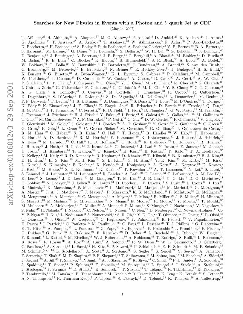
FIG. 1. Comparison of the data to the background prediction (dashed line), and the baseline SUSY model of Section VA 2(dotted line). The data consist of the 98 events of the γb data with 6Et > 20 GeV, except in b) which contains no 6Et

requirement. In each case the predictions have been normalized to the data. The distributions are: a) the photon Et, b) themissing Et, c) the b–tagged jet Et and d) the Et of the second jet with Et >15 GeV, if there is one. For display, the SUSYmodel event yield is scaled up by a factor of 4 for a), c) and d) and a factor of 40 for b).

11

02.5

57.510

12.515

17.520

0 200 400 600 800Ht (GeV)

Eve

nts/

27 G

eV

CDF 85pb-1

• γ+b+/Et Data

a) b)

c) d)

Backgroundχ~0

2 → γχ~0

1 model

0

10

20

30

40

50

0 50 100 150∆φ(γ-/Et)

Eve

nts/

12de

g

05

101520253035404550

0 2 4 6Njet

Eve

nts

0

10

20

30

40

50

0 50 100 150∆φ(jet-/Et)

Eve

nts/

12de

g

FIG. 2. Comparison of the data to the background prediction (dashed line), and the the baseline SUSY model of SectionVA 2 (dotted line), each normalized to the 98 events of the γb data with 6Et > 20 GeV. The distributions are: a) Ht (totalenergy), b) ∆φ between the photon and the 6Et, c) number of jets with Et > 15 GeV, and d) ∆φ between the missing Et andthe nearest jet. For display, the SUSY model event yield is scaled up by a factor of 4.

12

1

10

10 2

0 50 100 150 200 250 300 350 400 450M(γ,b) (GeV)

Eve

nts/

17 G

eV

• 85pb-1 CDF γ+b Data

Background estimate

FIG. 3. Comparison of the γb mass in the data to the background prediction (dashed line), normalized to the 1175 events ofthe γb data.

13

0

2468

101214

0 50 100 150 200 250 300 350 400 450M(b,jet) (GeV)

Eve

nts/

15 G

eV/c

2

CDF 85pb-1

• γ+b+/Et Data

a)

b)

Backgroundχ~0

2 → γχ~0

1 model

0246

8101214

0 100 200 300 400 500 600 700M(γ,b,jet) (GeV)

Eve

nts/

23 G

eV/c

2

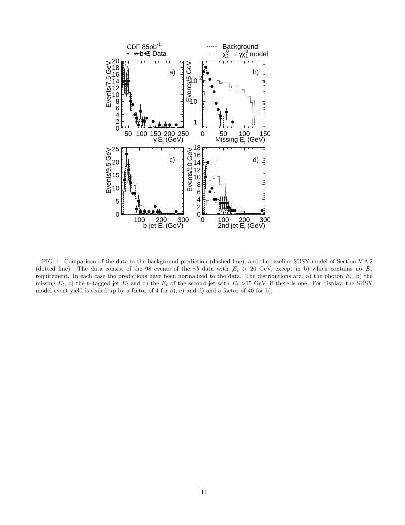
FIG. 4. The distributions for: a) M(b, j) and b) M(γ, b, j) for the 6Et > 20 GeV events as shown in Figure 5. Only 63 of the98 events have a second jet and make it into this plot. The data are compared to a background prediction (dashed line), andthe baseline SUSY model of Section VA 2 (dotted line), each normalized to the data. The Monte Carlo prediction is scaled upby a factor of 3.

14

A. Analysis of Events with Large Missing Et

Six events pass the a priori selection criteria requiring a photon, b–tag, and 6Et >40 GeV. Two of these events alsopass the ∆φ(γ − 6Et) < 168◦ requirement. We have examined these two events to see if there indications of anythingelse unusual about them (for example, a high–pt lepton, or a second jet which forms a large invariant mass with thefirst b-jet, to take signals of GMSB and Higgsino models respectively).

The first event (67537/59517) does not have the characteristics of a typical b-tag. It is a two-track tag (which hasa worse signal–to–noise) with the secondary vertex consistent with the beam pipe radius (typical of an interactionin the beam pipe). The two tracks have a pt of 2 and 60 GeV, respectively; this highly asymmetric configuration isunlikely if the source is a b–jet. There are several other tracks at the same φ as the jet that are inconsistent witheither the primary or secondary vertex. We conclude the b-tag jet in this event is most likely to be a fake, comingfrom an interaction in the beam pipe.

The second event has a typical b–tag but there are three jets, and all three straddle cracks in the calorimeter(η = 0.97,−1.19,−0.09), implying the 6Et is very likely to be mismeasured.

In both events we judge by scanning that the primary vertex is the correct choice so that a mismeasurement of the6Et due to selecting the wrong vertex is unlikely.

While we have scanned these two events and find they are most likely not true γb 6Et events, we do not excludethem from the event sample as the background calculations include these sources of mismeasured events.

Run/Event γ Et 6Et M(b, jet) b Et jets Et ∆φ(γ − 6Et) ∆φ(jnear − 6Et) Ht

60951/189718 121 42 57 61 67,26,15 177 11 342

64997/119085 222 44 97 173 47 170 1 495

63684/15166 140 57 63 35 25,20,15 175 6 388

67537/59517∗ 36 73 399 195 141,113,46,17 124 20 595

69426/104696 33 58 266 143 119 180 3 344

68464/291827∗ 93 57 467 128 155,69 139 16 405

TABLE IV. Characteristics of the six events with 6Et > 40 GeV; the two marked with an asterisk also pass the∆φ(γ − 6Et) < 168◦ requirement. All units are GeV except for ∆φ which is in degrees. The columns are the Et of thephoton in the event, the missing Et, the mass of the b-jet and the second highest Et jet in the event, the Et of the b jet, the Et

of the jets other than the b jet, the ∆φ between the photon and the missing Et, the ∆φ between the the missing Et and thenearest jet, and the Ht of the event (scalar sum of the Et, the missing Et and the pt of any muons in the event).

B. Analysis of Five High–mass Events

If the events include production of new, heavy particles, we might observe peaks, or more likely, distortions in thedistributions of the masses formed from combinations of objects. To investigate this, we create a scatter plot of themass of the b-quark jet and the second highest-Et jet versus the mass of the photon, b-quark jet and second highestjet in Figure 5 and 4.

As seen in the figures, the five events at highest M(b, j) seem to form a cluster on the tail of the distribution. Thereare 63 events in the scatter plot which are the subset of the 98 events with 6Et > 20 GeV which contain a second jet.The five events include the two (probable background) events with 6Et > 40 GeV and ∆φ(γ − 6Et) < 168◦ and threeevents with large Ht (> 400 GeV). Since these events were selected for their high mass, we expect they would appearin the tails of several of the distributions such as Ht. Table V shows the characteristics of these five events.

Run/Event γ Et 6Et M(b, jet) b Et jet Et’s ∆φ(γ − 6Et) ∆φ(jnear − 6Et) Ht

66103/52684 106 24 433 170 135,57 152 29 517

66347/373704 122 32 369 268 125,42 101 14 605

67537/59517 36 73 399 195 141,113,46,17 124 20 595

68333/233128 38 39 395 99 282,212 121 3 600

68464/291827 93 57 467 128 155,69 139 16 405

TABLE V. Characteristics of events with M(b, jet) > 300 GeV. For a complete description of the quantities, see Table IV.

15

In order to see if these events are significant, we need to make an estimate of the expected background. We definethe two regions indicated in Figure 5. The small box is placed so that it is close to the five events.1 This is intendedto maximize the significance of the excess. The large box is placed so that it is as far from the five events as possiblewithout including any more data events. This will minimize the significance. The two boxes can serve as informalupper and lower bounds on the significance. Since these regions were chosen based on the data, the excess overbackground cannot be used to prove the significance of these events. These estimates are intended only to give aguideline for the significance.

We cannot estimate the background to these five events using the CES and CPR methods described in Section III Adue to the large inherent statistical uncertainties in these techniques. We instead use the following procedure. Thelist of backgrounds in Section III defines the number of events from each source with no restriction on M(b, j). Wenormalize these numbers to the 63 events in the scatter plot. We next derive the fraction of each of these sources weexpect at high M(b, j). We multiply the background estimates by the fractions. The result is a background estimatefor the high–mass regions.

To derive the fractions of background sources expected at high M(b, j) we look at each background in turn. Thefake photons are QCD events where a jet has fluctuated into mostly electromagnetic energy. For this source we usethe positive Lxy background prediction [11] to provide the fraction. This prediction is derived from a QCD jet sampleby parameterizing the positive tagging probability as a function of several jet variables. The probability for each jetis summed over all jets for the untagged sample to arrive at a tagging prediction. Since the prediction is derived fromQCD jets we expect it to be reliable for these QCD jets also. Running this algorithm (called “Method 1” [11]) on theuntagged photon and 6Et sample yields the fraction of expected events in each of the two boxes. The fractions aresummarized in Table VI.

Source Big box Small box

fake γ 0.080 ± 0.007 0.017 ± 0.003

γ, fake tag 0.112 ± 0.009 0.032 ± 0.005

γbb 0.10 ± 0.03 0.022 ± 0.007

γcc 0.08 ± 0.04 0.018 ± 0.008

TABLE VI. The fraction of the 63 γbj 6Et events for each background expected to fall into the high–M(b, j) boxes defined inFigure 5.

1Note that events cannot be above the diagonal in the M(γ, b, j) − M(b, j) plane, so the true physical area is triangular.

16

The second background source considered consists of real photons with fake tags. We calculate this contributionusing the measured negative tagging rate applied to all jets (i.e. before b-tagging) in the sample. Finally, the realphoton and heavy flavor backgrounds are calculated based on the Monte Carlo. The results from estimating thefractions are shown in Table VI.

The estimates of the sources of background for the 63 events at all M(b, j) have statistical uncertainties, as dothe fractions in Table VI; we include both in the uncertainty in the number of events in the high–mass boxes. Wepropagate the systematic uncertainties on the backgrounds to the 63 events at all M(b, j) and include the followingsystematics due to the fractions:

1. 50% of the real photon and mistag background calculation for the possibility that the quark and gluon content,as well as the heavy flavor fraction, in photon events may differ from the content in QCD jets.

2. 50% of the real photon and mistag background calculation for the possibility that using the positive taggingprediction to correct the Monte Carlo for the 6Et cut may have a bias.

3. 100% of the real photon and real heavy flavor background calculation for the possibility that the tails in theMonte Carlo M(b, j) distribution may not be reliable.

The results of multiplying the backgrounds at all M(b, j) with the fractions expected at high M(b, j) are shown inTable VII.

Source Big box Small box

fake γ 3.3 ± 1.5 ± 0.5 0.70 ± 0.33 ± 0.10

γ, fake tag 0.97 ± 0.09 ± 0.69 0.28 ± 0.05 ± 0.20

γbb 0.75 ± 0.26 ± 1.18 0.16 ± 0.06 ± 0.26

γcc 0.44 ± 0.26 ± 0.79 0.11 ± 0.06 ± 0.17

total 5.5 ± 1.5 ± 1.6 1.24 ± 0.35 ± 0.38

TABLE VII. Summary of the estimates of the background at high M(b, j) in the boxes in the M(γ, b, j) − M(b, j) planedefined in Figure 5.

The result is that we expect 5.5 ± 1.5 ± 1.6 events in the big box, completely consistent with five observed. Weexpect 1.2 ± 0.35 ± 0.38 events in the small box. The probability of observing five in the small box is 1.6%, a 2.7σeffect, a posteriori.

We next address a method for avoiding the bias in deciding where to place a cut when estimating backgroundsto events on the tail of a distribution. This method was developed by the Zeus collaboration for the analysis of thesignificance of the tail of the Q2 distribution [18]. Figure 6 summarizes this method. The Poisson probability thatthe background fluctuated to the observed number of events (including uncertainties on the background estimate) isplotted for different cut values. We use the projection of the scatter plot onto the M(b, j) axis and make the cut onthis variable since this is where the effect is largest. We find the minimum probability is 1.4 × 10−3, which occursfor a cut of M(b, j) >400 GeV. We then perform 10,000 “pseudo-experiments” where we draw the data accordingto the background distribution derived above and find the minimum probability each time. We find 1.2% of theseexperiments have a minimum probability lower than the data, corresponding to a 2.7σ fluctuation. Including theeffect of the uncertainties in the the background estimate does not significantly change the answer.

We note that this method is one way of avoiding the bias from deciding in what region to compare data andbackgrounds after seeing the data distributions. It does not, however, remove the bias from the fact that we areinvestigating this plot, over all others, because it looks potentially inconsistent with the background. If we makeenough plots one of them will have a noticeable fluctuation. We conclude that the five events on the tail representsomething less than a 2.7σ effect.

17

0

50

100

150

200

250

300

350

400

450

500

0 100 200 300 400 500 600 700

1.2±0.35±0.38events expected

5.5±1.5±1.6events expected

CDF 85pb-1 γ+b+/Et Data

Data (large dots)and expectedbackground x10

M(γ,b,jet) (GeV)

M(b

,jet)

(G

eV)

a posteriori probability:minimum: 1.6%maximum: 58%

FIG. 5. M(b, j) versus M(γ, b, j) for the events with 6Et > 20 GeV as shown in Figure 5. Only 63 of the 98 events have asecond jet and make it into this plot. The small dots are the result of making the scatter plot for the untagged data (passingall other cuts) and weighting it with the positive tagging prediction. The estimates of background expected in the boxes arefound by the method described in the text.

18

10-2

10-1

1

10

0 50 100 150 200 250 300 350 400 450M(b,jet) Cut (GeV/c2)

Eve

nts

pass

ing

cut

CDF 85pb-1 γ+b+/Et Data

DataExpected background

10-3

10-2

10-1

1

0 50 100 150 200 250 300 350 400 450

M(b,jet) Cut (GeV/c2)

Pro

b(ob

serv

ed e

vent

s pa

ss c

ut)

Expect 1.2% of experimentsto have minimum probabilityless than 0.14%

FIG. 6. The upper plot is the number of events passing a cut on M(b, j) for the data and the positive tagging prediction. Thelower plot is the probability that the number of events passing a cut on M(b, j) is consistent with the positive tagging prediction.The expected number of experiments with such a low minimum probability is derived from 10,000 simulated experiments drawnfrom the distribution of the expected background.

19

C. Additional Objects in the Data Sample

We have searched the γb data sample for other unusual characteristics. The creation and decay of heavy squarks,for example, could produce an excess of events with multiple jets. In Figure 7 we histogram the number of eventswith N or more jets. Table VIII presents the numbers of events observed and expected. Some backgrounds arenegative due to the large statistical fluctuations of the fake photon background. When all backgrounds are includedthe distribution in the number of jets in the data is consistent with that from background.

Min Njet Observed, 6Et > 0 GeV Expected, 6Et > 0 GeV Observed, 6Et > 20 GeV Expected, 6Et > 20 GeV

1 1175 1040 ± 72 ± 172 98 77 ± 23 ± 20

2 464 394 ± 44 ± 63 63 39 ± 18 ± 12

3 144 82 ± 24 ± 14 25 −8 ± 12 ± 3

4 36 17 ± 11 ± 3 7 −

5 10 − 3 −

6 5 − 1 −

7 2 − 0 −

8 1 − 0 −

TABLE VIII. Numbers of events with N or more jets and the expected Standard Model background. Some backgroundpredictions are negative due to the large statistical fluctuations on the fake photon background method.

We have searched in the sample of events with a photon and b–tagged jet for additional high–Et objects using therequirements defined in Section II E. We find no events containing a second photon. We find no events containing ahadronic τ decay or a muon. We find one event with an electron; its characteristics are listed in Table IX. In scanningthis event, we note nothing else unusual about it.

We find 8 events of the 1175 which have a photon and b–tagged jet contain a second b–tagged jet with Et >30 GeV.(Out of the 1175, only 200 events have a second jet with Et >30 GeV.) Unfortunately, this is such a small samplethat we cannot use the background calculation to find the expected number of these events (the photon backgroundCES–CPR method returns 100% statistical uncertainties). One of the events with two tags has 30 GeV of missing Et

so is in the 98–event 6Et > 20 GeV sample.

Run/Event γ Et 6Et M(γ, e) b Et electron Et ∆φ(γ − 6Et) Ht

63149/4148 42 17 21 106 33 43 212

TABLE IX. Characteristics of the one event with a photon, tagged jet, and an electron.

20

0

200

400

600

800

1000

1200

0 2 4 6 8 10Minimum Njet

CDF 85pb-1

γ+b data

a)

Eve

nts

0

20

40

60

80

100

120

0 2 4 6 8 10

CDF 85pb-1

γ+b data/Et>20

Minimum Njet

b)

Eve

nts

FIG. 7. The distribution of the number of events with N or more jets, represented by the solid points. The boxes are centeredon the background prediction and their size reflects plus and minus one-σ of combined statistical and systematic uncertaintyon the background prediction. The distributions are: a) all events with a photon and b-tagged jet, b) all events with a photon,b-tagged jet and 6Et > 20 GeV. Some background predictions are negative due to the large statistical fluctuations on the fakephoton background method. The results are also tabulated in Table VIII.

21

V. LIMITS ON MODELS OF SUPERSYMMETRY

In the following sections we present limits on three specific models of supersymmetry [19]. Each of these modelspredicts significant numbers of events with a photon, a b–quark jet and missing transverse energy (i.e γb 6Et).

As is typical for supersymmetry models, each of these shows the problems in the process of choosing a model andpresenting limits on it. Each of these models is very specific and thus represents a very small area in a very largeparameter space. Consequently the odds that any of these is the correct picture of nature is small. They are currenttheories devised to address current concerns and may appear dated in the future. (This aspect is particularly relevantto the experimentalists, who often publish their data simultaneously with an analysis depending on a current model.)In addition these models can show sensistivity to small changes in the parameters.

The first model is based on a particular location in MSSM parameter space which produces the signature of γb 6Et+X .We consider both direct production of charginos and neutralinos and, as a second model, indirect production ofcharginos and neutralinos through squarks and gluinos. The third model is based on the gauge–mediated concept,discussed further below.

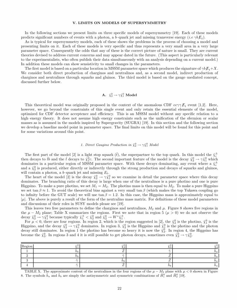
A. χ02 → γχ0

1 Model

This theoretical model was originally proposed in the context of the anomalous CDF eeγγ 6Et event [1,2]. Here,however, we go beyond the constraints of this single event and only retain the essential elements of the model,optimized for CDF detector acceptence and efficiency. This is an MSSM model without any specific relation to ahigh–energy theory. It does not assume high–energy constraints such as the unification of the sfermion or scalarmasses as is assumed in the models inspired by Supergravity (SUGRA) [19]. In this section and the following sectionwe develop a baseline model point in parameter space. The final limits on this model will be found for this point andfor some variations around this point.

1. Direct Gaugino Production in χ02 → γχ0

1 Model

The first part of the model [2] is a light stop squark (t), the superpartner to the top quark. In this model the χ±

i

then decays to tb and the t decays to χ01c. The second important feature of the model is the decay χ0

2 → γχ01 which

dominates in a particular region of MSSM parameter space. With these decays dominating, any event where a χ±

i

and a χ02 is produced, either directly or indirectly through the strong production and decays of squarks and gluinos,

will contain a photon, a b–quark jet and missing Et.The heart of the model [2] is the decay χ0

2 → γχ01 so we examine in detail the parameter space where this decay

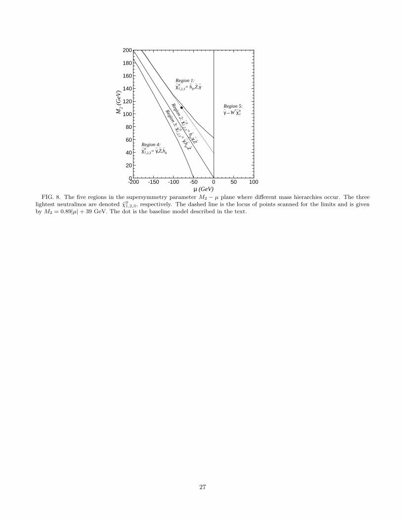
dominates. The branching ratio of this decay is large when one of the neutralinos is a pure photino and one is pureHiggsino. To make a pure photino, we set M1 = M2. The photino mass is then equal to M2. To make a pure Higgsinowe set tan β ≈ 1. To avoid the theoretical bias against a very small tanβ (which makes the top Yukawa coupling goto infinity before the GUT scale) we will use tanβ = 1.2. In this case, the Higgsino mass is approximately equal to|µ|. The above is purely a result of the form of the neutralino mass matrix. For definitions of these model parametersand discussions of their roles in SUSY models please see [19].

This leaves two free parameters to define the charginos and neutralinos, M2 and µ. Figure 8 shows five regions inthe µ − M2 plane; Table X summarizes the regions. First we note that in region 5 (µ > 0) we do not observe thedecay χ0

2 → γχ01 because typically χ±

1 < χ02 and χ0

2 → W ∗χ±

1 .For µ < 0, there are four regions. In region 2, which is the region suggested in [2], the χ0

2 is the photino, χ01 is the

Higgsino, and the decay χ02 → γχ0

1 dominates. In region 3, χ02 is the Higgsino and χ0

1 is the photino and the photondecay still dominates. In region 1 the photino has become so heavy it is now the χ0

3. In region 4, the Higgsino hasbecome the χ0

3. In regions 3 and 4 it is still possible to get photon decays, sometimes even χ03 → γχ0

2.

Region χ01 χ0

2 χ03 χ0

4

1 hb Z γ ha

2 hb γ Z ha

3 γ hb Z ha

4 γ Z hb ha

TABLE X. The approximate content of the neutralinos in the four regions of the µ − M2 plane with µ < 0 shown in Figure8. The symbols ha and hb are simply the antisymmetric and symmetric combinations of H0

1 and H02 [19].

22

We choose to concentrate on region 2 where the photon plus b decay signature can be reliably estimated by theMonte Carlo event generator PYTHIA [20]. The χ0

2 → γχ01 decay dominates here. We also note that in this region the

cross section for χ±

2 χ02 is 3–10 times larger than the cross section for χ±

1 χ02 even though the χ±

2 is significantly heavier

than the χ±

1 . This is due to the large W component of the χ±

2 .Since region 2 is approximately one-dimensional, we scan in only one dimension, along the diagonal, when setting

limits on χ±

2 χ02 production. To decide where in the region to place the model, we note that the mass of χ0

2 equalsM2 and the mass of χ0

1 = |µ| in this region. To give the photon added boost for a greater sensitivity, we will set M2

significantly larger than |µ|. This restricts us to the upper part of region 2. The dotted line in Figure 8 is the set ofpoints defined by all these criteria and is given by M2 = 0.89 ∗ |µ| + 39 GeV.

The next step is to choose a t mass. It is necessary that χ01 < t < χ±

1 for the decay χ±

1 , χ±

2 → bt to dominate.We find that in Region 2, χ±

1 ≈ M2. If the t mass is near the χ±

1 , the b will only have a small boost, but the χ01 in

the decay t → cχ01 will have a greater boost, giving greater 6Et. If the t mass is near the χ0

1, the opposite occurs.In Monte Carlo studies, we find considerably more sensitivity if the t mass is near the χ0

1. We set the t mass to beMχ0

1

+5 GeV. Since the χ±

2 χ02 production cross section is larger than χ±

1 χ02 and will be detected with better efficiency,

when we simulate direct production we set the Monte Carlo program to produce only χ±

2 χ02 pairs. The final limit

is expressed as a cross section limit plotted versus the χ±

2 mass (which is very similar to the χ02 mass). This model

is designed to provide a simple, intuitive signature that is not complicated by branching ratios and many modes ofproduction.

For the baseline model, we chose a value of µ near the exclusion boundary of current limits [21] on a t which decaysto cχ0

1. The point we chose is Mχ0

1

= 80 GeV. From the above prescription, this corresponds to Mχ0

1

= −µ = 80 GeV,

Mχ0

2

= Mχ±

1

= M2 = 110 GeV, and Mt = 85 GeV. This point, indicated by the dot in Figure 8, gives the lightest

mass spectrum with good mass splittings that is also near the exclusion boundary from LEP and DO Collaborations.

2. Squarks and Gluinos

Now we address the squarks and gluinos, which can produce χ±

i χ02 in their decays, and sleptons, which can appear

in the decays of charginos and neutralinos.We will set the squarks (the lighter b and both left and right u, d, s and c) to 200 GeV and the gluino to 210 GeV.

The heavier t and b are above 1 TeV. The gluino will decay to the squarks and their respective quarks. The squarks willdecay to charginos or neutralinos and jets. This will maximize the production of χ±

i χ02 and therefore the sensitivity.

This brings us to the limit on indirect production in the χ02 → γχ0

1 model. The chargino and neutralino parametersare fixed at the baseline model parameters. We then vary the gluino mass and set the squark mass according toMg = MQ + 10 GeV. The limit is presented as a limit on cross section plotted versus the gluino mass. When

the gluino mass crosses the tt threshold at 260 GeV, the gluino can decay to tt and production of χ±

i χ02 decreases.

However, since all squarks are lighter than the gluino, the branching ratio to the t is limited and production will notfall dramatically.

Some remaining parameters of the model are now addressed. Sleptons could play a role in this model. They havesmall cross sections so they are not often directly produced, but if the sleptons are lighter than the charginos, thecharginos can decay into the sleptons. In particular, the chargino decay tb may be strongly suppressed if it competeswith a slepton decay. We therefore set the sleptons to be very heavy so they do not compete for branching ratios. Weset MA large. The lightest Higgs turns out to be only 87 GeV due to the corrections from the light third–generationsquarks. This is below current limits so we attempted to tune the mass to be heavier and found it was difficult toachieve, given the light t and low tanβ.

Using the PYTHIA Monte Carlo program, we find that 69% of all events generated with squarks and gluinos havethe decay χ0

2 → γχ01, 58% have the decay χ±

i → tb, and 30% have both. (To be precise, the light stop squark wasexcluded from this exercise, as it decays only to cχ0

1. A light stop pair thus gives the signature cc + 6Et, one of thesignatures used to search for it, [21,22] but not of interest here.)

23

3. Acceptances and Efficiencies

This section describes the evaluation of the acceptance and efficiency for the indirect production of χ±

i χ0i through

squarks and gluinos and the direct production of χ±

2 χ02 in the MSSM model of χ0

2 → γχ01. We use the PYTHIA Monte

Carlo with the CTEQ4L parton distribution functions (PDFs) [23]. The efficiencies for squark and gluino productionat the baseline point are listed in Table XI.

Cuts Cumulative Efficiency (%)

Photon Et > 25 GeV,|η| < 1.0, ID cuts 50One jet Et,corr > 30 GeV, |η| < 2.0 47

One SVX tag Et,corr > 30 GeV, |η| < 2.0 4.36Et > 40 GeV 2.9

TABLE XI. Efficiencies for the baseline point with squark and gluino production. The efficiencies do not include branchingratios.

24

The total efficiencies, which will be used to set production limits below, are listed in Table XII for the productionof χ±

i χ0i through squarks and gluinos, and in Table XIII for direction production. Typical efficiencies are 2-3% in the

former case, and 1% in the latter.

4. Systematic Uncertainty

Some systematics are common to the indirect production and the direct production. The efficiencies of the isolationrequirement in the Monte Carlo and Z → e+e− control sample cannot be compared directly due to differences in theEt-spectra of the electromagnetic cluster, and the multiplicity and Et spectra of associated jets. The difference (14%)is taken to be the uncertainty in the efficiency of the photon identification cuts. The systematic uncertainty on theb–tagging efficiency (9%) is the statistical uncertainty in comparisons of the Monte Carlo and data. The systematicuncertainty on the luminosity (4%) reflects the stability of luminosity measurements.

We next evaluate systematics specifically for the indirect production. The baseline parton distribution function isCTEQ4L. Comparing the efficiency with this PDF to the efficiencies obtained with MRSD0′ [24] and GRV–94LO [25]for the squark and gluino production, we find a standard deviation of 5%. Turning off initial– and final–state radiation(ISR/FSR) in the Monte Carlo increases the efficiency by 1% and 2% respectively and we take half of these as therespective systematics. Varying the jet energy scale by 10% causes the efficiency to change by 4%. In quadrature, thetotal systematic for the indirect production is 18%.

Evaluating the same systematics for the direct production, we find the uncertainty from the choice of PDF is 5%,from ISR/FSR is 2%/9%, and from jet energy scale is 4%. In quadrature, the total systematic uncertainty for thedirect production is 20%.

5. Limits on the χ02 → γχ0

1 Model, Indirect Production

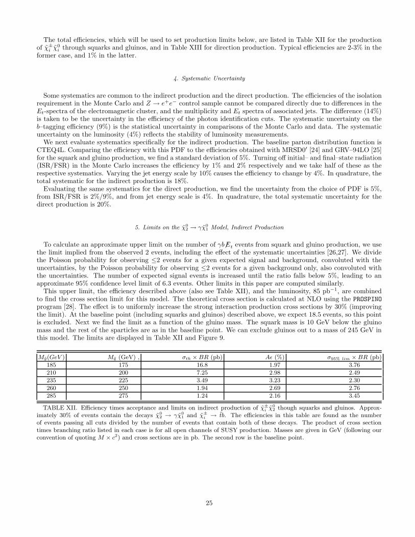
To calculate an approximate upper limit on the number of γb 6Et events from squark and gluino production, we usethe limit implied from the observed 2 events, including the effect of the systematic uncertainties [26,27]. We dividethe Poisson probability for observing ≤2 events for a given expected signal and background, convoluted with theuncertainties, by the Poisson probability for observing ≤2 events for a given background only, also convoluted withthe uncertainties. The number of expected signal events is increased until the ratio falls below 5%, leading to anapproximate 95% confidence level limit of 6.3 events. Other limits in this paper are computed similarly.

This upper limit, the efficiency described above (also see Table XII), and the luminosity, 85 pb−1, are combinedto find the cross section limit for this model. The theoretical cross section is calculated at NLO using the PROSPINO

program [28]. The effect is to uniformly increase the strong interaction production cross sections by 30% (improvingthe limit). At the baseline point (including squarks and gluinos) described above, we expect 18.5 events, so this pointis excluded. Next we find the limit as a function of the gluino mass. The squark mass is 10 GeV below the gluinomass and the rest of the sparticles are as in the baseline point. We can exclude gluinos out to a mass of 245 GeV inthis model. The limits are displayed in Table XII and Figure 9.

Mg(GeV ) Mq (GeV) , σth × BR (pb) Aǫ (%) σ95% lim × BR (pb)

185 175 16.8 1.97 3.76

210 200 7.25 2.98 2.49

235 225 3.49 3.23 2.30

260 250 1.94 2.69 2.76

285 275 1.24 2.16 3.45

TABLE XII. Efficiency times acceptance and limits on indirect production of χ±

i χ02 though squarks and gluinos. Approx-

imately 30% of events contain the decays χ02 → γχ0

1 and χ±

i → tb. The efficiencies in this table are found as the numberof events passing all cuts divided by the number of events that contain both of these decays. The product of cross sectiontimes branching ratio listed in each case is for all open channels of SUSY production. Masses are given in GeV (following ourconvention of quoting M × c2) and cross sections are in pb. The second row is the baseline point.

25

6. Limits on the χ02 → γχ0

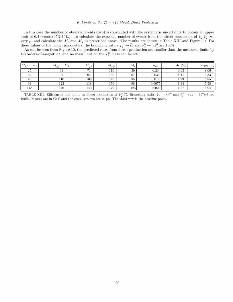
1 Model, Direct Production

In this case the number of observed events (two) is convoluted with the systematic uncertainty to obtain an upperlimit of 6.4 events (95% C.L.). To calculate the expected number of events from the direct production of χ±

2 χ02, we

vary µ, and calculate the Mt and M2 as prescribed above. The results are shown in Table XIII and Figure 10. Forthese values of the model parameters, the branching ratios χ±

2 → tb and χ02 → γχ0

1 are 100%.As can be seen from Figure 10, the predicted rates from direct production are smaller than the measured limits by

1-3 orders-of-magnitude, and no mass limit on the χ±

2 mass can be set.

Mχ0

1

= −µ Mχ0

2

= M2, Mχ±

1

Mχ±

2

Mt σth Aǫ (%) σ95% lim

25 61 71 110 30 0.23 0.93 8.06

62 95 94 130 67 0.034 1.41 5.33

79 110 108 140 85 0.018 1.29 5.85

93 123 118 150 98 0.0075 1.34 5.58

118 146 140 170 123 0.0022 1.27 5.94

TABLE XIII. Efficiencies and limits on direct production of χ±

2 χ02. Branching ratios χ0

2 → γχ01 and χ±

i → tb → (χ01c)b are

100%. Masses are in GeV and the cross sections are in pb. The third row is the baseline point.

26

0

20

40

60

80

100

120

140

160

180

200

-200 -150 -100 -50 0 50 100

Region 5:γ~→W*χ

~±1

Region 1:χ~0

1,2,3= h~

b,Z~,γ~

Region 4:χ~0

1,2,3= γ~,Z~,h~

b

Region 2: χ ~01,2,3 =

h ~b ,γ ~

,Z ~

Region 3: χ ~01,2,3 =

γ ~,h ~

b ,Z ~

M2

(GeV

)

µ (GeV)FIG. 8. The five regions in the supersymmetry parameter M2 − µ plane where different mass hierarchies occur. The three

lightest neutralinos are denoted χ01,2,3, respectively. The dashed line is the locus of points scanned for the limits and is given

by M2 = 0.89|µ| + 39 GeV. The dot is the baseline model described in the text.

27

1

10

160 180 200 220 240 260 280 300

85pb-1 γ+b+/Et Data

Gluino Mass (GeV/c2)

Cro

ss S

ectio

n x

BR

(pb

)

χ~0

2 → γχ~0

1 modelSquark and gluino productionM(q

~)=M(g

~)-10 GeV

M(χ~0

1)=80 GeV, M(χ~0

2)=110 GeV

M(χ~±

2)=140 GeV, M(t~)=85 GeV

95% C.L. Limit Theory (NLO)

FIG. 9. The limits on the cross section times branching ratio for SUSY production of γb 6Et events in the χ02 → γχ0

1 model.All production processes have been included; the dominant mode is the production of squarks and gluinos which decay tocharginos and neutralinos. The overall branching ratio to the γb 6Et topology is approximately 30%.

28

10-3

10-2

10-1

1

10

10 2

10 3

10 4

100 120 140 160 180

85pb-1 γ+b+/Et Data

χ~±

2 Mass (GeV/c2)

Cro

ss S

ectio

n x

BR

(pb

)

χ~±

2 χ~0

2 production

χ~0

2 → γχ~0

1 model

M(t~)=M(χ

~01)+5 GeV

95% C.L. Limit Theory

FIG. 10. The limits on the χ±

2 χ02 cross section in the χ0

2 → γχ01 SUSY model. The branching ratios χ0

2 → γχ01 and

χ±

i → tb → (χ01c)b are taken to be 100%.

29

B. Gauge-mediated Model

This is the second SUSY model [19] which can give substantial production of the signature γb 6Et. In this model thedifference between the mass of the standard model particles and their SUSY partners is mediated by gauge (the usualelectromagnetic, weak, and strong) interactions [29] instead of gravitational interactions as in SUGRA models. SUSYis assumed broken in a hidden sector. Messenger particles gain mass through renormalization loop diagrams whichinclude the hidden sector. SUSY particles gain their masses through loops which include the messenger particles.

This concept has the consequence that the strongly–interacting squarks and gluinos are heavy and the right-handedsleptons are at the same mass scale as the lighter gauginos. A second major consequence is that the gravitino is verylight (eV scale) and becomes the LSP. The source of b quarks is no longer the third generation squarks, but the decays

of the lightest Higgs boson. If the lightest neutralino is mostly Higgsino, the decay χ01 → hG can compete with the

decays χ01 → ZG and χ0

1 → γG. The Higgs decays to bb as usual. Since SUSY particles are produced in pairs, eachevent will contain two cascades of decays down to two χ0

1’s, each of which in turn will decay by one of these modes. Ifone decays to a Higgs and one decays to a photon, the event will have the signature of a photon, at least one b–quarkjet, and missing Et.

We will use a minimal gauge-mediated model with one exception. This MGMSB model has five parameters, withthe following values:

• Λ = 61 − 90 TeV, the effective SUSY-breaking scale;

• M/Λ = 3, where M is the messenger scale;

• N = 2 the number of messenger multiplets;

• tanβ = 3;

• the sign of µ < 0.

We will compute the MGMSB model using the GMSB option of ISAJET [30]. We then re–enter the model using theMSSM options so that we can make one change: we set µ = −0.75M1. This makes the lightest neutralino a Higgsinoso the branching ratio for χ0

1 → hG will be competitive with χ01 → γG. We produce all combinations of χ±

i and χ0j ,

which are the only significant cross sections. We vary Λ which varies the overall mass scale of the supersymmetricparticles.

The model masses and branching ratios are given in Table XIV. The branching ratio is defined as the number ofevents with χ0

1 → γG and χ01 → hG divided by the number of events produced from all sources predicted by the

model. We are using ISAJET with the CTEQ4L parton distribution function. The first point appears to have anunusually large efficiency because of other sources for b quarks which are not reflected in the definition of the signalbranching ratio. We use the systematic uncertainties evaluated using the direct production of the χ0

2 → γχ01 model.

Taking the two events observed, and convoluting with a 20% systematic uncertainty gives an upper limit of 6.4events observed at 95% C.L. The final limits on this model are presented in Table XV and displayed in Figure 11.Again, one can see that the experimental sensitivity is not adequate to set a mass limit (this time on the χ±

1 mass)by several orders of magnitude.

30

Mχ0

1

, Mχ0

2

Mχ±

1

BR(χ01 → γG) BR(χ0

1 → hG)

113 141 130 90 2

132 157 147 62 18

156 178 170 33 40

174 194 186 22 50

TABLE XIV. The models used in the limits on the GMSB scenario. The lightest Higgs boson is 100 GeV. The masses arein GeV and the branching ratios are in %.

Aǫ BR σth × BR σ95% lim × BR

27.4 3 0.010 0.27

7.5 20 0.0402 1.00

8.4 23 0.0230 0.89

11.4 18 0.0111 0.66

TABLE XV. Efficiencies and limits on direct production of χ±

i χ0j in the GMSB scenario. Branching ratios are not included

in these efficiencies. The first row has an inflated efficiency due to the definition of the branching ratio. The units of Aǫ andthe branching ratio are % and the cross sections are in pb.

31

10-3

10-2

10-1

1

10

10 2

10 3

120 140 160 180 200

85pb-1 γ+b+/Et Data

χ~±

1 Mass (GeV/c2)

Cro

ss S

ectio

n x

BR

(pb

)

χ~±

i χ~0

i productionGMSB Modelχ~0

1 → γG or χ~0

1 → hG

95% C.L. Limit

Theory

FIG. 11. The limits on the cross section times branching ratio for SUSY production of γb 6Et events in the GMSB model. Allproduction processes have been included.

VI. MODEL–INDEPENDENT LIMITS

As described in the introduction, there are several advantages to presenting limits of searches in a model–independentform. In the previous sections we derived limits on models of supersymmetry and presented the results as a limiton a cross section times branching ratio for a specific model, (σ × BR)lim = N lim/LAǫ, where Nlim is the 95%confidence level on the number of events of anomalous production and L is the integrated luminosity. We make adistinction between the acceptance, A, which is defined as probability that an object passes Et, η, and ∆φ cuts,and the efficiency, ǫ, which is the probability of events surviving all other sources of inefficiencies, such as photonidentification cuts or b–tagging requirements, which is detector-specific. The acceptance may be calculated fromkinematic and geometric criteria alone, so an experienced worker in the field can compute it using only a MonteCarlo event generator program, while the efficiency requires access to the full detector simulation and, typically,multiple control samples. In our formulation, Nlim includes the degradation in sensitivity due to uncertainties on Aǫ,luminosity, and background subtractions, when they are included, as well as the statistical upper limit on the numberof events.

In the case of model–independent limits, there is no model to determine the efficiency and therefore we reporta limit on (σ × BR × Aǫ)lim = N lim/L. These limits, which are presented in the next section, do not have animmediate interpretation. (They do imply, however, a cross section range that we are not sensitive to, even withperfect efficiency.) In order to determine the meaning of these limits, in particular if a model is excluded or not, theremust still be a mechanism for an interested physicist to calculate Aǫ for the model, and we develop three methods inthe Appendix.

A. Model–independent Limits on γbX Signatures

The limit on (σ × BR × Aǫ)limi = N lim/L is described by reporting that two events are observed with an isolated

photon with Et >25 GeV and |η| < 1, a SVX-tagged b–quark jet with Et >30 GeV and |η| < 2, ∆φ(γ−6Et) < 168◦ and6Et > 40 GeV. The cuts are fully described in Section II. The integrated luminosity for this sample is (85 ± 3) pb−1.

The resulting 95% confidence level limit on (σ ×BR ×Aǫ)lim for the γb 6Et signature is then 0.069 pb. Adding the4% luminosity uncertainty we find the cross section limit increases to 0.070 pb. If we also add the 22% uncertainty inAǫ from the WW limits (a typical uncertainty on an efficiency for this signature) discussed in the Appendix, we findthe cross section limit increases 10% to 0.077 pb. This is the final model–independent limit on the signature γb 6Et.

32

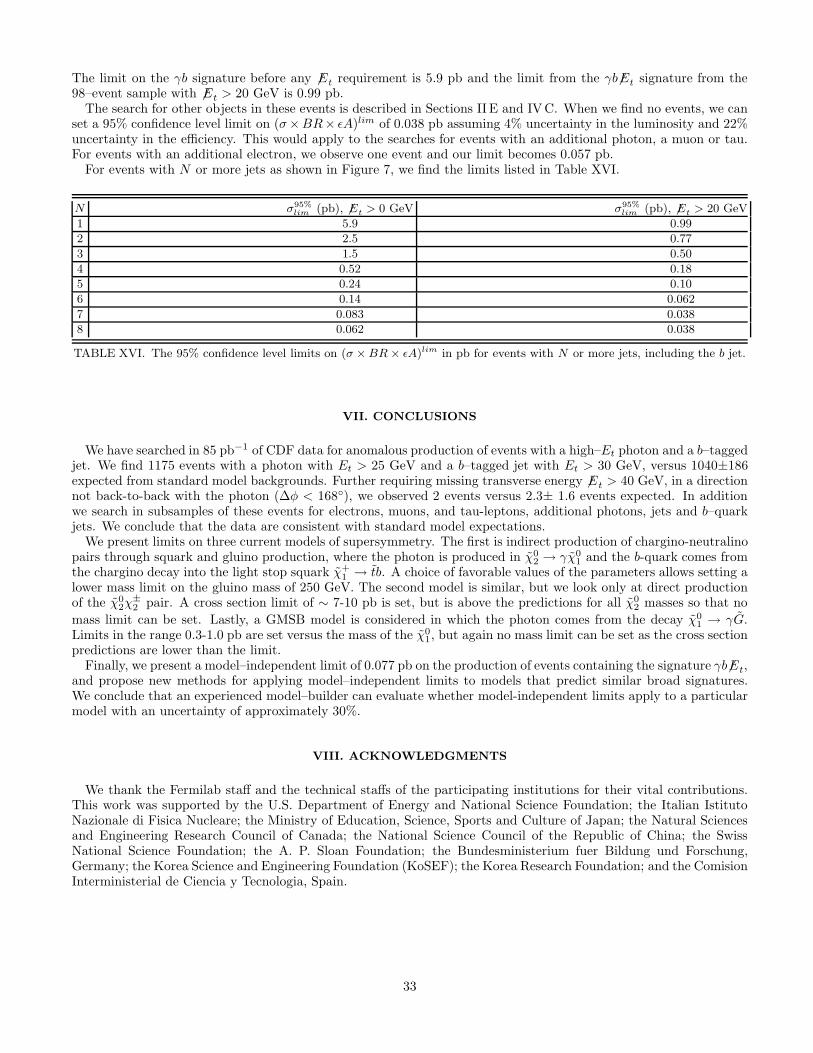
The limit on the γb signature before any 6Et requirement is 5.9 pb and the limit from the γb 6Et signature from the98–event sample with 6Et > 20 GeV is 0.99 pb.

The search for other objects in these events is described in Sections II E and IVC. When we find no events, we canset a 95% confidence level limit on (σ×BR× ǫA)lim of 0.038 pb assuming 4% uncertainty in the luminosity and 22%uncertainty in the efficiency. This would apply to the searches for events with an additional photon, a muon or tau.For events with an additional electron, we observe one event and our limit becomes 0.057 pb.

For events with N or more jets as shown in Figure 7, we find the limits listed in Table XVI.

N σ95%

lim (pb), 6Et > 0 GeV σ95%

lim (pb), 6Et > 20 GeV

1 5.9 0.99

2 2.5 0.77

3 1.5 0.50

4 0.52 0.18

5 0.24 0.10

6 0.14 0.062

7 0.083 0.038

8 0.062 0.038

TABLE XVI. The 95% confidence level limits on (σ × BR × ǫA)lim in pb for events with N or more jets, including the b jet.

VII. CONCLUSIONS

We have searched in 85 pb−1 of CDF data for anomalous production of events with a high–Et photon and a b–taggedjet. We find 1175 events with a photon with Et > 25 GeV and a b–tagged jet with Et > 30 GeV, versus 1040±186expected from standard model backgrounds. Further requiring missing transverse energy 6Et > 40 GeV, in a directionnot back-to-back with the photon (∆φ < 168◦), we observed 2 events versus 2.3± 1.6 events expected. In additionwe search in subsamples of these events for electrons, muons, and tau-leptons, additional photons, jets and b–quarkjets. We conclude that the data are consistent with standard model expectations.

We present limits on three current models of supersymmetry. The first is indirect production of chargino-neutralinopairs through squark and gluino production, where the photon is produced in χ0

2 → γχ01 and the b-quark comes from

the chargino decay into the light stop squark χ+1 → tb. A choice of favorable values of the parameters allows setting a

lower mass limit on the gluino mass of 250 GeV. The second model is similar, but we look only at direct productionof the χ0

2χ±

2 pair. A cross section limit of ∼ 7-10 pb is set, but is above the predictions for all χ02 masses so that no

mass limit can be set. Lastly, a GMSB model is considered in which the photon comes from the decay χ01 → γG.

Limits in the range 0.3-1.0 pb are set versus the mass of the χ01, but again no mass limit can be set as the cross section

predictions are lower than the limit.Finally, we present a model–independent limit of 0.077 pb on the production of events containing the signature γb 6Et,

and propose new methods for applying model–independent limits to models that predict similar broad signatures.We conclude that an experienced model–builder can evaluate whether model-independent limits apply to a particularmodel with an uncertainty of approximately 30%.

VIII. ACKNOWLEDGMENTS

We thank the Fermilab staff and the technical staffs of the participating institutions for their vital contributions.This work was supported by the U.S. Department of Energy and National Science Foundation; the Italian IstitutoNazionale di Fisica Nucleare; the Ministry of Education, Science, Sports and Culture of Japan; the Natural Sciencesand Engineering Research Council of Canada; the National Science Council of the Republic of China; the SwissNational Science Foundation; the A. P. Sloan Foundation; the Bundesministerium fuer Bildung und Forschung,Germany; the Korea Science and Engineering Foundation (KoSEF); the Korea Research Foundation; and the ComisionInterministerial de Ciencia y Tecnologia, Spain.

33

IX. APPENDIX: APPLICATION OF MODEL–INDEPENDENT LIMITS

In the body of this paper, we present the limits on specific models of new physics that predict the γb 6Et signature,then rigorously calculate Aǫ for that model by using a Monte Carlo with a full detector simulation. We present ourlimits on (σ × BR)lim = N lim/LAǫ, or a parameter of the model such as the mass of a supersymmetric particle.

A new paradigm, the signature–based or, equivalently, model–independent search may be an effective method forreporting the results of searches in the future. In this case, a signature, such as the photon and b–quark jet addressedin this paper, is the focus of the search rather than the predictions of a particular model.

There are several advantages to this approach [1,3,4].

1. The results are not dated by our current theoretical understanding.

2. No a priori judgement is necessary to determine what is an interesting model.

3. The results more closely represent the experimental observations and results will be presented in a form thatcan be applied to a broad range of models including those not yet imagined.

4. The number of signatures is more reasonably limited than the number of models and model parameters.

5. Concentrating on a particular model can tend to focus the search very narrowly, ignoring variations on thesignature which may be just as likely to yield a discovery.

6. Time spent on studying models can be diverted to systematically searching additional signatures.

In order to reflect the data results more generally, in the body of this paper we also present a limit on (σ × BR ×Aǫ)lim = N lim/L for the signatures with no calculation of Aǫ. With limits presented this way, the collaboration itself,model–builders and other interested workers are no longer given limits on the physics models directly but now mustderive the limits themselves. This has the potential for a wider application of the limits. In a pratical sense, it meansthe interested workers must calculate Aǫ for the model under study.

In this Appendix, we present three methods to calculate Aǫ. These results together with the model-independentlimits can be used to set limits on most models that predict events with the γb 6Et signature.

The three methods are referred to as “object efficiencies”, “standard model calibration process,” and “public MonteCarlo”. In the sections below we describe each in turn. In the following sections, we test these methods by comparingthe results of each Aǫ calculation to the rigorously–derived Aǫ for the specific supersymmetry models.

A. Object Efficiencies

The first method for deriving Aǫ to use in conjunction with the model–independent limits is object efficiencies.The person investigating a model would run a Monte Carlo generator and place the acceptance cuts on the outputwhich will determine the acceptance, A. The next step would be to apply efficiencies (simple scale factors) for theidentification of each object in the signature, such as the photon or the b-quark tag. This has the advantage of beingbeing very straightforward and the disadvantage that correlations between the objects in the event are not accountedfor. For example, a model with many jets would tend to have a lower efficiency for the photon isolation requirementthan a model with few jets and this effect would not be reflected in this estimate of the efficiency.

Using a sample of Z → e+e− events to measure the efficiencies of the global event cuts, we find the z < 60 cm cutis 92% efficient. The probability of finding no energy out-of-time is 98%. In this case the total global efficiency wouldbe the product of these two efficiencies. In the discussion below, the efficiency of the identification of each object isoften listed as efficiencies of several separate steps which should be multiplied to find the total efficiency.

We can also use Z → e+e− events to measure the efficiency of the photon identification cuts. One electron fromthe Z is required to fire the trigger, but the second electron is unbiased with respect to the trigger. In addition theZ peak indicates the number of true physics events, ideal for measuring efficiencies. Which Z electron is required topass which set of cuts (trigger or offline) must be effectively randomized to avoid correlations between the two setsof cuts. Requiring the cluster to be far from the boundary of the active area in the calorimeters is 73% efficient [31].The trigger is 91% efficient, the identification cuts are 86% and the isolation requirement is 77% efficient.

For the b–quark efficiency we use a 70% probability that the jets from the event are contained in the SVX. (Thiswould be 64% if the global event vertex was not already required to have z < 60 cm.) We add a 90% probability that

34

the jet was taggable (containing two reconstructed tracks in the SVX, passing pt cuts) and apply the published [32]tagging probability as a function of the jet Et which can be summarized as

0 for Et < 18 GeV0.35 + 0.00277 ∗ Et for 18 < Et < 72 GeV

0.6 for Et > 72 GeV

The missing Et is found as the vector sum of the noninteracting particles in the event. As long as the missing Et

is large, the resolution on the 6Et should not greatly effect the efficiency.In Section IVC, we searched the events in the γb sample for additional leptons; here we present approximate object

efficiencies for those cuts. These requirements and their efficiencies are borrowed from top–quark analyses [11,12] as arepresentative selection for high–Et leptons. The efficiencies quoted here are measured in those contexts and thereforethey are approximations in a search for new physics. In particular, the isolation efficiency is likely to be dependenton the production model. For example, if a model of new physics contained no jets, then the isolation efficiency islikely to be greater than that measured in top–quark events which contain several jets on average.

For the electron search we require Et > 25 GeV and |η| < 1.0. Given that an electron, as reported in the output ofthe Monte Carlo generator, passes these acceptance cuts, the probability that the electron strikes the calorimeter wellaway from any uninstrumented region is 87%, the probability to pass identification cuts is 80%, and to pass isolationcuts is approximately 87% [31].

For muons we require pt > 25 GeV and |η| <1.0. Given that the muon, as reported in the output of the MonteCarlo generator, passes these cuts, the fiducial acceptance of the muon detectors is 48%. Once the muon is accepted,the probability to pass identification cuts is 91%, and to pass isolation cuts is approximately 81%.

Tau leptons are identified only in their one– and three–prong hadronic decays which have a branching ratio of 65%.(Tau semileptonic decays can contribute to the electron and muon searches.) We require that the calorimeter clusterhas Et > 25 GeV and |η| < 1.2 and the object is not consistent with an electron or muon. Given that the τ decaysto a one– or three–prong hadronic decay mode and passes the Et and η requirements, the probability that the taupasses identification and isolation cuts is approximately 57%.

In Section IXD we apply these object efficiencies to the supersymmetry models and compare to the results of therigorously–derived efficiency to test the accuracy of the results.

B. Standard Model Calibration Process

The second method for determining Aǫ for a model is the Standard Model process or efficiency model. In this methodwe select a simple physics model that produces the signature. The model is purely for the purpose of transmittinginformation about Aǫ so it does not have any connection to a model of new physics. Since it may be considered acalibration model, it does not have to be tuned and will not become dated. The interested model builder runs aMonte Carlo of the new physics and places acceptance cuts on the output, determining A, the same as the first stepin the object efficiencies method. This result is then multiplied by the value of ǫ which is taken to be the same as thevalue of ǫ which we report here for the standard model process.

We have adopted WW production as our efficiency model. One W is required to decay to eν and we replace theelectron with a photon before the detector simulation. The second W is forced to decay to bu, so the combinationyields the signature γb 6Et. Since some efficiencies may be dependent on the Et of the objects in the event, we willvary the “W” mass to present this effect. A model–builder would then choose the efficiency that most closely matchesthe mass scale of the new physics models.

35

The Aǫ for this model is found using the same methods as used for the models of supersymmetry. From thedifference in the observed efficiencies in Monte Carlo and data Z → ee samples, we use a 14% uncertainty on theefficiency of the photon ID and isolation. We use 9% for the b–tagging efficiency uncertainty. The parton distributionfunction we use is CTEQ4L. Comparing this efficiency to those obtained with the MRSD0′ and GRV–94LO partondistribution functions, we find a standard deviation of 5%. Turning off initial– and final–state radiation increasesthe efficiency by 2% and 23% respectively and we take half these numbers as the systematic uncertainty. Varyingthe jet energy scale by 10% causes the efficiency to change by 6%. We use an 4% uncertainty for the luminosity. Inquadrature, the total systematic is 22%. Table XVII summarizes the results.

MW 75 GeV 100 GeV 125 GeV 150 GeV 175 GeV

ǫA(%) 0.85 2.56 4.86 6.98 8.12

ǫ (%) 11.8 10.7 13.9 15.4 16.5

TABLE XVII. Summary of the efficiencies found for the values of W mass used in the WW calibration model versus thevalue of the “W” mass.

36

In Section IXD we apply this method of calculating Aǫ to the supersymmetry models and compare to the resultsof the rigorously–derived efficiency to test the accuracy of the results.

C. A Public Monte Carlo

A Monte Carlo event generator followed by a detector simulation is the usual method for determining the efficiencyof a model of new physics. However, there is usually considerable detailed knowledge required to run the simulationprograms correctly so it is not practical to allow any interested person access to it. But if the simulation is greatlysimplified while still approximating the full program, it could become usable for any worker in the field. The model–builder then only has to run this simple Monte Carlo to determine Aǫ.

An example of this kind of detector simulation, called SHW, was developed for the Fermilab Run II SUSY/HiggsWorkshop [33]. Generated particles are traced to a calorimeter and energy deposited according to a simple fractionalacceptance and Gaussian resolution. A list of tracks is also created according to a simple efficiency and resolutionmodel, and similarly for muon identification. The calorimeter energy is clustered to find jets. Electromagnetic clusters,together with requirements on isolation and tracking, form electron and photon objects. The tagging of b–quarks isdone with a simple, parameterized efficiency. At points where object identification efficiencies would occur, such asa χ2 cut on an electron shower profile, the appropriate number of candidates are rejected to create the inefficiency.The result is a simple list of objects that are reconstructed for each event. This method of determining efficienciesaddresses the largest concern not addressed in the previous methods – the correlation of the characteristics of jets inthe model with isolation requirements. We note that a highly parameterized Monte Carlo has obvious limitations.

We have used the SHW program to compute efficiencies for the three models considered above. Since the programis tuned to provide the approximate efficiency of the Run II detector, we made a few minor changes to reflect the RunI detector. In particular, we changed the photon fiducial efficiency from 85% to 73% and the offline efficiency from85% to 60%. We reduced the SVX acceptance along the z axis from 60 cm to 31 cm. Finally, we removed soft leptonb-tagging and added a 90% efficiency for the global event cuts.

In the next section we use the public Monte Carlo to calculate Aǫ for the supersymmetry models and compare theresults to the rigorously–derived efficiency to test the accuracy of the public Monte Carlo.

D. Tests of the Model–independent Efficiency Methods

In the body of this paper we have provided rigorous limits on several variations of three supersymmetry physicsmodels that produce the signature of γb 6Et. In this section we apply the model-independent efficiency methods tothe supersymmetry models. We can then compare the results with the rigorous limits to evaluate how effective it isto apply the model–independent limits to real physics models.

In most cases we need to distinguish between acceptance and efficiency. Acceptance, indicated by A, we define asthe probability for generated Monte Carlo objects to pass all geometric and Et cuts. For the γb 6Et signature, with6Et defined as the vector sum of neutrinos and LSP’s, the cuts defining the acceptance of the signature are listed inTable XVIII.

γ Et > 25 GeV |η| <1.0

b–quark Et > 30 GeV |η| <2.0

Additional Signatures

Σpt(ν, LSP ) 6Et > 40 GeV,∆φ(γ − 6Et) < 168◦

e Et > 25 GeV |η| <1.0

µ Et > 25 GeV |η| <1.0

τ Et > 25 GeV |η| <1.2

2nd γ Et > 25 GeV |η| <1.0

2nd b Et > 30 GeV |η| <2.0

Jets Et > 15 GeV |η| <2.0

TABLE XVIII. The list of requirements on the output of a Monte Carlo generator which define the acceptance of a signature,A. The requirements on the photon and b–quark jet above the double line are common to all signatures in this paper. Whenmissing Et is required, as in all the supersymmetry searches and the tests of model–independent methods, both 6Et >40 GeVand ∆φ(γ − 6Et) < 168◦ are required. The 6Et requirement is removed and other requirements are added to make specificsubsamples.

37

Table XIX and Figure 12 list the results. The columns marked R are the efficiency times acceptance done rigorously,divided by the the same found using each of the model–independent methods. The difference of this ratio from 1.0one is a measure of the accuracy of the approximate methods compared to the rigorous method.

Model Ms BR(%) A A · ǫ Robj RWW RSHW

130 3 65.0 27.50 2.79 3.03 1.07GMSB 147 20 49.8 7.45 0.91 1.00 0.70

Ms = Mχ±

1

170 23 51.7 8.35 0.97 1.00 0.87

186 18 54.7 11.44 1.26 1.22 1.11

185 30 17.0 1.97 0.91 0.68 0.48χ0

2 → γχ01 210 30 22.0 2.98 1.04 0.73 0.90

q, g production 235 30 24.0 3.23 1.01 0.68 0.90Ms = Mg 260 30 24.5 2.69 0.82 0.52 0.75

285 30 19.7 2.16 0.84 0.48 0.72

110 100 13.5 0.93 0.54 0.54 0.59χ0

2 → γχ01 130 100 12.6 1.41 0.88 0.80 0.87

q, g production 140 100 14.8 1.29 0.68 0.60 0.66Ms = M

χ±

2

150 100 13.7 1.34 0.77 0.65 0.78

170 100 11.5 1.27 0.85 0.68 0.65

TABLE XIX. The results of comparing the methods of calculating Aǫ using the model–independent methods and therigorously–derived Aǫ. Each row is a variation of a model of supersymmetry as indicated by the label in the first column andthe mass of a supersymmetric particle listed in column two (GeV). The column labeled A is the acceptance of the model in %and the next column is the rigorously–derived Aǫ. The columns labeled with R are the ratios of the rigorously–derived Aǫ toAǫ found using the model–independent method indicated.

38

0

0.5

1

1.5

2

2.5

3

0 2 4 6 8 10 12 14 16

Monte Carlo/SHW

Monte Carlo/Per Object

Monte Carlo/Effic. Model

Monte Carlo/Kinematic

Aε(

Mon

te C

arlo

)/A

ε(m

etho

d)

Model numberFIG. 12. The ratio of the efficiencies obtained with full detector simulation to those obtained with the model–independent

methods. The x axis is the row number from Table XIX.

E. Conclusions from tests

There are several notable effects apparent immediately from Table XIX and Figure 12. The first is that thecomparison of efficiencies for one model point fares especially poorly. This occurs when the branching ratio for themodel is very small (2%). When the events do not contain many real photons and b quarks, the small number ofobjects misidentified as photons and b-quarks becomes important. For example, jets may pass photon cuts and cquarks may be b-tagged. When this occurs, the full simulation will be more efficient than a method which specificallyrequires that the Monte Carlo generate an isolated photon or b-quark in order to accept the event. This is true of theobject efficiencies method and the efficiency model method. We note that the public Monte Carlo method does allowmisidentification and so it does not show this large mismatch. We can conclude that when the branching ratios aresmall, the public Monte Carlo method is vastly superior to the others.

In the object efficiency method, the acceptance of the signature is computed by running the Monte Carlo withouta detector simulation. As each object in the signature is identified and passes acceptance cuts, the individual objectefficiencies are multiplied. These object efficiencies which may or may not be Et– or η–dependent, are listed in SectionIXA. In this test, these efficiencies are typically well–matched to the rigorously–derived efficiencies. The average ofRobj over all models except the first, is 0.88 ± 0.21 where 0.21 is the RMS computed with respect to 1.0, the idealresult.

In the efficiency model method, we generate a Monte Carlo model that is not related to a search for new physicsbut produces the signature of interest. For the signature of γb 6Et, we generated WW → (γν)(bu). The efficiencymodel results are also optimistic, the average is a ratio of 0.74±0.35 where again the uncertainty is actually the RMSwith 1.0, the ideal result. We found that the difficulty of applying this method was in choosing the mass scale. Forexample, we chose to match the “W” mass to the χ±

2 mass in the direct production of the χ02 → γχ0

1 model. However,the photon comes from a secondary decay and the effect of the LSP mass compared to the massless neutrino causesthe Et of the γ and b to be poorly matched to the Et of these objects in the WW model.

In the public Monte Carlo method, we compute the efficiency using SHW, a highly-parameterized, self–containedMonte Carlo. In general, results here are somewhat optimistic with the average ratio to the rigorous total efficiencybeing 0.77 ± 0.28, where the uncertainty is the RMS computed with respect to 1.0, the ideal result.

For completeness we also include the ratio of the simple acceptance to the rigorous acceptance times efficiency. Theaverage ratio is 0.12 ± 0.87.

The methods for calculating efficiency without access to the full detector simulation are accurate to approximately30% overall. They tend to underestimate Aǫ by 10-25% but the result for individual comparisons varies greatly. Theseuncertainties are larger than, but not greatly larger than, a typical uncertainty in a rigorously–derived efficiency, which

39

is 20%.We conclude that to determine if a model is easily excluded or far from being excluded by the data, the model–

independent methods are sufficient. If the model is within 30% of exclusion, no conclusion can be drawn and theefficiency should be rigorously–derived.

40

[1] F. Abe et al. (The CDF Collaboration), Phys. Rev. Lett. 81 1791 (1998), Phys. Rev. D 59 092002,1999.[2] S. Ambrosanio, G.L. Kane, Graham D. Kribs, Stephen P. Martin, and S. Mrenna, Phys. Rev. Lett. 76, 3498 (1996); G. L.

Kane and S. Mrenna, Phys. Rev. Lett. 77, 3502 (1996); S. Ambrosanio, G.L. Kane, Graham D. Kribs, Stephen P. Martin,and S. Mrenna, Phys. Rev. D 55, 1372 (1997).

[3] H. Frisch, in proceedings of the NATO Summer School 1998, Cargese, France, to be published, edited by P. Binetruy adG. Smadja (Kluwer Academic Publishers).

[4] B. Abbott et al. (The DO Collaboration), Phys. Rev. D 62, 92004 (2000); B. Abbott et al. (The DO Collaboration), Phys.Rev. Lett., 86, 3712 (2001); B. Abbott et al. (The DO Collaboration), to be published in Phys. Rev. D, hep-ex/0011067(2000).

[5] F. Abe et al. (The CDF Collaboration), Phys. Rev. Lett 83, 3124 (1999).[6] F. Abe et al. (The CDF Collaboration), Nucl. Instrum. Methods Phys Res., Sect. A 271, 387 (1988).[7] D. Amidei et al., Nucl. Instrum. Methods Phys. Res., Sect. A 350, 73 (1994).[8] The CDF coordinate system is right-handed, and has the z axis aligned with the proton beam and y vertical. The azimuthal

angle is denoted as φ and the polar angle as θ; η is − ln[tan(θ/2)].[9] D. Amidei et al., Nucl. Instrum. Methods Phys. Res., Sect. A 269, 51 (1988).

[10] F. Abe et al. (The CDF Collaboration), Phys. Rev. D 45, 1448 (1992).[11] F. Abe et al. (The CDF Collaboration), Phys. Rev. Lett. 74 2626 (1995); Phys. Rev. D 50, 2966 (1994).[12] F. Abe et al. (The CDF Collaboration), Phys. Rev. Lett. 79, 3585 (1997).[13] F. Abe et al. (The CDF Collaboration), Phys. Rev. Lett. 73, 2662 (1994); Phys. Rev. D 48, 2998 (1993).[14] F. Abe et al. (The CDF Collaboration), Phys. Rev. D 50, 2966 (1994); Phys. Rev. Lett. 73, 225 (1994).[15] The γbb and γcc Monte Carlo program was incorporated into Herwig by M. Mangano, based on calcuations in R. K. Ellis

and Z. Kunszt, Nucl. Phys. B 303, 653 (1988); R. K. Ellis and P. Nason, Nucl. Phys. B 312, 551 (1989).[16] F. Abe et al. (The CDF Collaboration), Phys. Rev. Lett. 73, 2662 (1994).[17] In this Letter when two uncertainties are reported, the first is statistical and the second is systematic.[18] J. Breitweg et al. (The ZEUS Collaboration), Z. Phys. C74 207, 1997. A similar method was developed in C. Adloff et al.

(The H1 Collaboration), Z. Phys. C74 191, 1997.[19] For an introduction to SUSY, see, for example: M. Carena, R.L. Culbertson, S. Eno, H.J. Frisch, and S. Mrenna, The

Search for Supersymmetry at the Tevatron Collider, Rev. Mod. Phys. 71, no.4 (July 1999).[20] T. Sjostrand, Computer Physics Commun. 82, 74 (1994). We use Version 6.1.[21] S. Abachi et al. (The DO Collaboration), Phys. Rev. Lett. 76 2222 (1996); G. Abbiendi et al. (The OPAL Collaboration),

Phys. Lett. B 456, 95 (1999); P. Abreu et al. (The Delphi Collaboration), Phys. Lett. B 496, 59 (2000); M. Acciarri et al.

(The L3 Collaboration), Phys. Lett. B 471, 308 (1999); R. Barate et al. (The Aleph Collaboration), Phys. Lett. B 434,189 (1998).

[22] T. Affolder et al. (The CDF Collaboration) Phys. Rev. Lett. 84, 5704 (2000).[23] H. L. Lai et al. (The CTEQ collaboration), Phys. Rev. D 55, 1280 (1997).[24] A. D. Martin, R. G. Roberts, and W. J. Stirling, Phys. Lett. B 306, 145 (1993).[25] M. Gluck, E. Reya, and A. Vogt, Z. Phys. C 67, 433 (1995).[26] O. Helene, Nucl Instrum. Methods Phys. Res., Sect. A 212, 319 (1983).[27] G. Zech, Nucl Instrum. Meth. A 277, 608 (1989).[28] W. Beenaker, R. Hopker, and M. Spira, hep–ph/9611232 (1996).[29] For an introduction to gauge-mediated SUSY, see, for example: S. Dimopoulos, S. Thomas, and J. D. Wells, Nucl. Phys.

B 488 39 (1997); R. L. Culbertson et al., hep–ph/0008070 (2000).[30] H. Baer et al., Proc. of the Workshop on Physics at Current Accelerators and the Supercollider, Argonne, 703 (1993). We

are using Version 7.37.[31] D. Toback Ph.D. thesis, University of Chicago, 1997.[32] Weiming Yao, in New Directions for High–Energy Physics, proceedings of 1996 DPF / DPB Summer Study on New

Directions for High–energy Physics (Snowmass 96), Snowmass, CO, edited by D.G. Cassel and L. Trindle (Stanford, CA,Stanford Linear Accelerator Center, 1997. 2v.).

[33] The Supersymmetry/Higgs Workshop, Fermilab, Batavia IL, November 19, 1998. http://fnth37.fnal.gov/susy.html.

41