arX

iv:h

ep-p

h/96

0135

9v2

11

Dec

199

6

SLAC–PUB–7106hep-ph/9601359

January, 1996

CALCULATING SCATTERING AMPLITUDES EFFICIENTLY⋆

LANCE DIXON

Stanford Linear Accelerator Center

Stanford University, Stanford, CA 94309

ABSTRACT

We review techniques for more efficient computation of perturbative scattering am-plitudes in gauge theory, in particular tree and one-loop multi-parton amplitudes inQCD. We emphasize the advantages of (1) using color and helicity information todecompose amplitudes into smaller gauge-invariant pieces, and (2) exploiting theanalytic properties of these pieces, namely their cuts and poles. Other useful toolsinclude recursion relations, special gauges and supersymmetric rearrangements.

Invited lectures presented at the Theoretical Advanced Study Institutein Elementary Particle Physics (TASI 95): QCD and Beyond

Boulder, CO, June 4-30, 1995

⋆Research supported by the US Department of Energy under grant DE-AC03-76SF00515.

1 Motivation

Feynman rules for covariant perturbation theory have been around for almostfifty years, and their adaptation to nonabelian gauge theories has been fully de-veloped for almost twenty-five years. Surely by now every significant standardmodel scattering process ought to have been calculated to the experimentally-required accuracy. In fact, this is far from the case, especially for QCD, whichis the focus of this school and of these lectures. Many QCD cross-sections havebeen calculated only to leading order (LO) in the strong coupling constant αs,corresponding to the square of the tree-level amplitude. Such calculations havevery large uncertainties — often a factor of two — which can only be reducedto reasonable levels, say 10% or so, by including higher-order corrections inαs.

Currently, no quantities have been computed beyond next-to-next-to-lead-ing-order (NNLO) in αs, and the only quantities known at NNLO are totallyinclusive quantities such as the total cross-section for e+e− annihilation intohadrons, and various sum rules in deep inelastic scattering. Many more pro-cesses have been calculated at next-to-leading-order (NLO), but at presentresults are still limited to where the basic process has four external legs, suchas a virtual photon or Z decaying to three jets, or production of a pair of jets(or a weak boson plus a jet) in hadronic collisions via qq → gg (qq → Wg),etc.

This is not to say that processes with more external legs are not interest-ing; they are of much interest, both for testing QCD in different settings andas backgrounds to new physics processes. For example, αs could be measuredat the largest possible momentum transfers using the ratio of three-jet eventsto two-jet events at hadron colliders, if only the three-jet process were knownat NLO. As another example, QCD is a major background to top quark pro-duction in pp collisions. If both t’s decay hadronically (t → Wb → qq′b), thebackground is from six jet production. Despite the fact that the QCD processstarts off at α6

s, it completely swamps the top signal. If one of the two topquarks decays leptonically (t → Wb → ℓνℓb), then QCD production of a Wplus three or four jets forms the primary background. This background pre-vented discovery of the top quark at the Tevatron in this channel, until theadvent of b tagging.1 Although the NLO corrections to three-jet productionare within sight, we are still far from being able to compute the top quarkbackrounds at NLO accuracy; on the other hand, it’s good to have long rangegoals.

These lectures are about amplitudes rather than cross-sections. The goalof the lectures is to introduce you to efficient techniques for computing tree

2

and one-loop amplitudes in QCD, which serve as the input to LO and NLOcross-section calculations. (The same techniques can be applied to many non-QCD multi-leg processes as well.) Zoltan Kunszt will then describe in detailhow to combine amplitudes into cross-sections.2

Efficient techniques for computing tree amplitudes have been available forseveral years, and an excellent review exists.3 One-loop calculations are con-siderably more involved — they form an “analytical bottleneck” to obtainingnew NLO results — and benefit from additional techniques. In principle itis straightforward to compute both tree and loop amplitudes by drawing allFeynman diagrams and evaluating them, using standard reduction techniquesfor the loop integrals that are encountered. In practice this method becomesextremely inefficient and cumbersome as the number of external legs grows,because there are:

1. too many diagrams — many diagrams are related by gauge invariance.

2. too many terms in each diagram — nonabelian gauge boson self-interactions are complicated.

3. too many kinematic variables — allowing the construction of arbitrarilycomplicated expressions.

Consequently, intermediate expressions tend to be vastly more complicatedthan the final results, when the latter are represented in an appropriate way.

In these lectures we will stress the advantages of (1) using color and he-licity information to decompose amplitudes into smaller (and simpler) gauge-invariant pieces, and (2) exploiting the analytic properties of these pieces,namely their cuts and poles. In this way one can tame the size of intermediateexpressions as much as possible on the way to the final answer. There aremany useful technical steps and tricks along the way, but I believe the overallorganizational philosophy is just as important. A number of the techniquescan be motivated by how calculations are organized in string theory.4,5 I willnot attempt to describe string theory here, but I will mention some placeswhere it provides a useful heuristic guide.

The approach advocated here is quite useful for multi-parton scatteringamplitudes. For more inclusive processes — for example the e+e− → hadronstotal cross-section — where the number of kinematic variables is smaller, andthe real and virtual contributions are on a more equal footing, the compu-tational issues are completely different, and the philosophy of splitting theproblem up into many pieces may actually be counterproductive.

3

2 Total quantum-number management (TQM)

The organizational framework mentioned above uses all the quantum-numbersof the external states (colors and helicity) to decompose amplitudes into sim-pler pieces; thus we might dub it “Total Quantum-number Management”.TQM suggests that we:

• Keep track of all possible information about external particles — namely,helicity and color information.

• Keep track of quantum phases by computing the transition amplitude ratherthan the cross-section.

• Use the helicity/color information to decompose the amplitude into simpler,gauge-invariant pieces, called sub-amplitudes or partial amplitudes.

• In many cases we may also introduce still simpler auxiliary objects, calledprimitive amplitudes, out of which the partial amplitudes are built.

• Exploit the “effective” supersymmetry of QCD tree amplitudes, and usesupersymmetry at loop-level to help manage the spins of particles propagatingaround the loop.

• Square amplitudes to get probabilities, and sum over helicities and colors toobtain unpolarized cross-sections, only at the very end of the calculation.

Carrying out the last step explicitly would generate a large analytic expression;however, at this stage one would typically make the transition to numericalevaluation, in order to combine the virtual and real corrections. The use ofTQM is hardly new, particularly in tree-level applications3 — but it becomesespecially useful at loop level.

2.1 Color management

First we describe the color decomposition of amplitudes,6,7 and review somediagrammatic techniques8 for efficiently carrying out the necessary group the-ory. The gauge group for QCD is SU(3), but there is no harm in generalizingit to SU(Nc); indeed this makes some of the group theory structure more ap-parent. Gluons carry an adjoint color index a = 1, 2, . . . , N2

c − 1, while quarksand antiquarks carry an Nc or N c index, i, = 1, . . . , Nc. The generators ofSU(Nc) in the fundamental representation are traceless hermitian Nc × Nc

matrices, (T a) i . We normalize them according to Tr(T aT b) = δab in order to

avoid a proliferation of√

2’s in partial amplitudes. (Instead the√

2’s appearin intermediate steps such as the color-ordered Feynman rules in Fig. 5.)

The color factor for a generic Feynman diagram in QCD contains a factorof (T a)

i for each gluon-quark-quark vertex, a group theory structure constantfabc — defined by [T a, T b] = i

√2 fabc T c — for each pure gluon three-vertex,

4

and contracted pairs of structure constants fabef cde for each pure gluon four-vertex. The gluon and quark propagators contract many of the indices togetherwith δab, δ

i factors. We want to first identify all the different types of colorfactors (or “color structures”) that can appear in a given amplitude, and thenfind rules for constructing the kinematic coefficients of each color structure,which are called sub-amplitudes or partial amplitudes.

The general color structure of the amplitudes can be exposed if we firsteliminate the structure constants fabc in favor of the T a’s, using

fabc = − i√2

(

Tr(

T aT bT c)

− Tr(

T aT cT b)

)

, (1)

which follows from the definition of the structure constants. At this stage wehave a large number of traces, many sharing T a’s with contracted indices, of theform Tr

(

. . . T a . . .)

Tr(

. . . T a . . .)

. . . Tr(

. . .). If external quarks are present,then in addition to the traces there will be some strings of T a’s terminatedby fundamental indices, of the form (T a1 . . . T am) ı1

i2. To reduce the number of

traces and strings we “Fierz rearrange” the contracted T a’s, using

(T a) 1i1

(T a) 2i2

= δ 2i1

δ 1i2

− 1

Ncδ 1i1

δ 2i2

, (2)

where the sum over a is implicit.Equation 2 is just the statement that the SU(Nc) generators T a form the

complete set of traceless hermitian Nc ×Nc matrices. The −1/Nc term imple-ments the tracelessness condition. (To see this, contract both sides of Eq. 2with δ i1

1 .) It is often convenient to consider also U(Nc) = SU(Nc) × U(1)gauge theory. The additional U(1) generator is proportional to the identitymatrix,

(T aU(1)) i =

1√Nc

δ i ; (3)

when this is added back the U(Nc) generators obey Eq. 2 without the −1/Nc

term. The auxiliary U(1) gauge field is often called the photon, because it iscolorless (it commutes with SU(Nc), faU(1)bc = 0, for all b, c) and therefore itdoes not couple directly to gluons; however, quarks carry charge under it. (Itscoupling strength has to be readjusted from QCD to QED strength for it torepresent a real photon.)

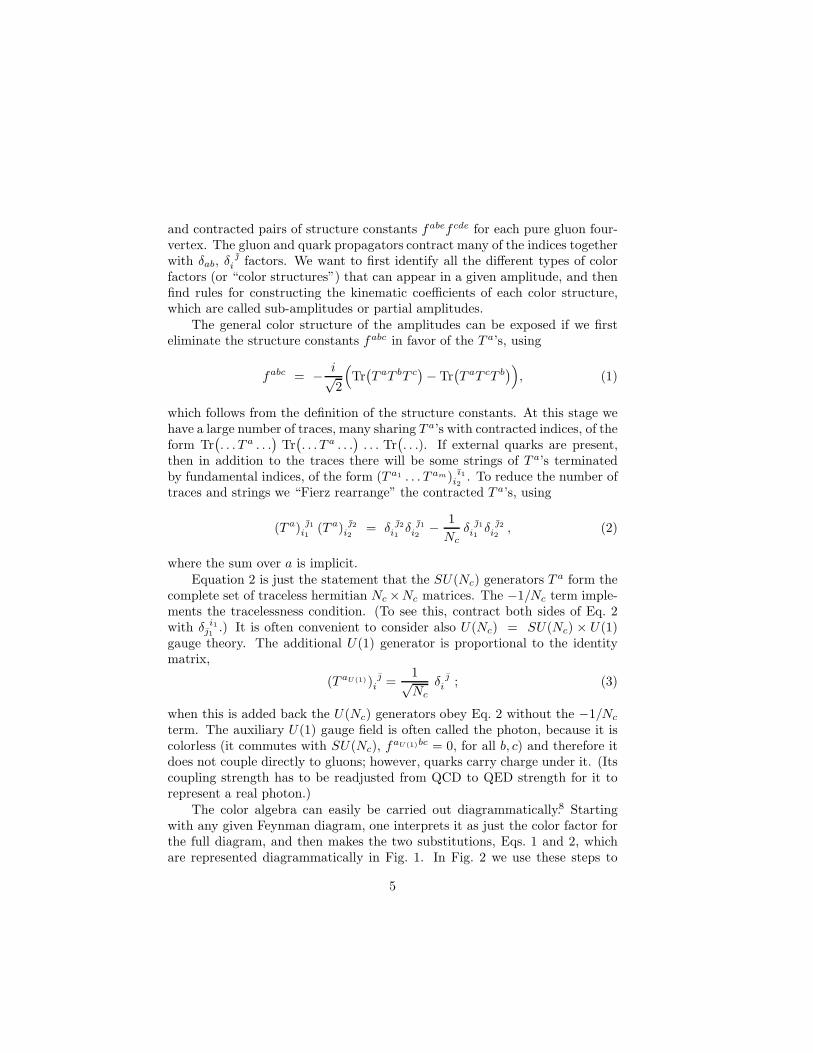
The color algebra can easily be carried out diagrammatically.8 Startingwith any given Feynman diagram, one interprets it as just the color factor forthe full diagram, and then makes the two substitutions, Eqs. 1 and 2, whichare represented diagrammatically in Fig. 1. In Fig. 2 we use these steps to

5

Figure 1: Diagrammatic equations for simplifying SU(Nc) color algebra. Curly lines (“gluonpropagators”) represent adjoint indices, oriented solid lines (“quark propagators”) representfundamental indices, and “quark-gluon vertices” represent the generator matrices (T a)

i.

simplify a sample diagram for five-gluon scattering at tree level. The final lineis the diagrammatic representation of a single trace, Tr

(

T a1T a2T a3T a4T a5)

,plus all possible permutations. Notice that the −1/Nc terms in Eq. 2 do notcontribute here, because the photon does not couple to gluons.

It is easy to see that any tree diagram for n-gluon scattering can be re-duced to a sum of “single trace” terms. This observation leads to the colordecomposition of the the n-gluon tree amplitude,6

Atreen ({ki, λi, ai}) = gn−2

∑

σ∈Sn/Zn

Tr (T aσ(1) · · ·T aσ(n)) Atreen (σ(1λ1 ), . . . , σ(nλn)).

(4)

Here g is the gauge coupling ( g2

4π = αs), ki, λi are the gluon momenta andhelicities, and Atree

n (1λ1 , . . . , nλn) are the partial amplitudes, which contain allthe kinematic information. Sn is the set of all permutations of n objects, whileZn is the subset of cyclic permutations, which preserves the trace; one sumsover the set Sn/Zn in order to sweep out all distinct cyclic orderings in thetrace. The real work is still to come, in calculating the independent partialamplitudes Atree

n . However, the partial amplitudes are simpler than the fullamplitude because they are color-ordered: they only receive contributions fromdiagrams with a particular cyclic ordering of the gluons. Because of this, thesingularities of the partial amplitudes, poles and (in the loop case) cuts, canonly occur in a limited set of momentum channels, those made out of sums ofcyclically adjacent momenta. For example, the five-point partial amplitudesAtree

5 (1λ1 , 2λ2 , 3λ3 , 4λ4 , 5λ5) can only have poles in s12, s23, s34, s45, and s51,and not in s13, s24, s35, s41, or s52, where sij ≡ (ki + kj)

2.

6

Figure 2: A sample diagram for tree-level five-gluon scattering, reduced to a single trace.

Similarly, tree amplitudes qqgg · · · g with two external quarks can be re-duced to single strings of T a matrices,

Atreen = gn−2

∑

σ∈Sn−2

(T aσ(3) · · ·T aσ(n)) 1i2

Atreen (1λ1

q , 2λ2q , σ(3λ3), . . . , σ(nλn)),

(5)where numbers without subscripts refer to gluons.Exercise: Write down the color decomposition for the tree amplitude qqQQg.

Color decompositions at loop level are equally straightforward. In Fig. 3we simplify a sample diagram for four-gluon scattering at one loop. Again the−1/Nc terms in Eq. 2 are not present, but now both single and double tracestructures are generated, leading to the one-loop color decomposition,7

A1−loopn ({ki, λi, ai})

= gn

[

∑

σ∈Sn/Zn

Nc Tr (T aσ(1) · · ·T aσ(n)) An;1(σ(1λ1 ), . . . , σ(nλn))

+

⌊n/2⌋+1∑

c=2

∑

σ∈Sn/Sn;c

Tr (T aσ(1) · · ·T aσ(c−1)) Tr (T aσ(c) · · ·T aσ(n))

× An;c(σ(1λ1 ), . . . , σ(nλn))

]

, (6)

where An;c are the partial amplitudes, Zn and Sn;c are the subsets of Sn thatleave the corresponding single and double trace structures invariant, and ⌊x⌋is the greatest integer less than or equal to x.

7

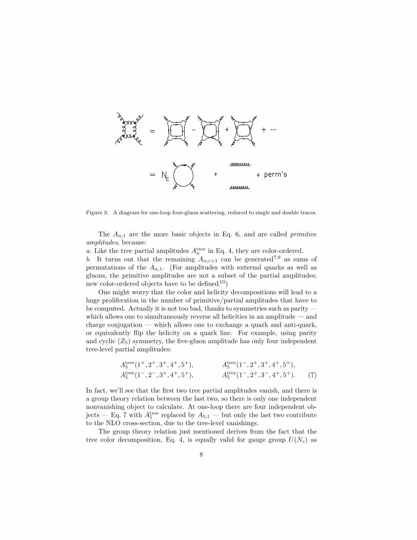
Figure 3: A diagram for one-loop four-gluon scattering, reduced to single and double traces.

The An;1 are the more basic objects in Eq. 6, and are called primitiveamplitudes, because:a. Like the tree partial amplitudes Atree

n in Eq. 4, they are color-ordered.b. It turns out that the remaining An;c>1 can be generated7,9 as sums ofpermutations of the An;1. (For amplitudes with external quarks as well asgluons, the primitive amplitudes are not a subset of the partial amplitudes;new color-ordered objects have to be defined.10)

One might worry that the color and helicity decompositions will lead to ahuge proliferation in the number of primitive/partial amplitudes that have tobe computed. Actually it is not too bad, thanks to symmetries such as parity —which allows one to simultaneously reverse all helicities in an amplitude — andcharge conjugation — which allows one to exchange a quark and anti-quark,or equivalently flip the helicity on a quark line. For example, using parityand cyclic (Z5) symmetry, the five-gluon amplitude has only four independenttree-level partial amplitudes:

Atree5 (1+, 2+, 3+, 4+, 5+), Atree

5 (1−, 2+, 3+, 4+, 5+),

Atree5 (1−, 2−, 3+, 4+, 5+), Atree

5 (1−, 2+, 3−, 4+, 5+). (7)

In fact, we’ll see that the first two tree partial amplitudes vanish, and there isa group theory relation between the last two, so there is only one independentnonvanishing object to calculate. At one-loop there are four independent ob-jects — Eq. 7 with Atree

5 replaced by A5;1 — but only the last two contributeto the NLO cross-section, due to the tree-level vanishings.

The group theory relation just mentioned derives from the fact that thetree color decomposition, Eq. 4, is equally valid for gauge group U(Nc) as

8

SU(Nc), but any amplitude containing the extra U(1) photon must vanish.Hence if we substitute the U(1) generator — the identity matrix — into theright-hand-side of Eq. 4, and collect the terms with the same remaining colorstructure, that linear combination of partial amplitudes must vanish. We get

0 = Atreen (1, 2, 3, . . . , n) + Atree

n (2, 1, 3, . . . , n) + Atreen (2, 3, 1, . . . , n)

+ · · · + Atreen (2, 3, . . . , 1, n), (8)

often called a “photon decoupling equation”7 or “dual Ward identity”3 (becauseEq. 8 can be derived from string theory, a.k.a. dual theory). In the five-pointcase, we can use Eq. 8 to get

Atree5 (1−, 2+, 3−, 4+, 5+) = −Atree

5 (1−, 3−, 2+, 4+, 5+)

−Atree5 (1−, 3−, 4+, 2+, 5+)

−Atree5 (1−, 3−, 4+, 5+, 2+). (9)

The partial amplitude where the two negative helicities are not adjacent hasbeen expressed in terms of the partial amplitude where they are adjacent, asdesired.

Since color is confined and unobservable, the QCD-improved parton modelcross-sections of interest to us are averaged over initial colors and summedover final colors. These color sums can be performed very easily using thediagrammatic techniques. For example, Fig. 4 illustrates the evaluation ofthe color sums needed for the tree-level four-gluon cross-section. In this casewe can use the much simpler U(Nc) color algebra, omitting the −1/Nc termin Eq. 2, because the U(1) contribution vanishes. (This shortcut is not validfor general loop amplitudes, or if external quarks are present.) Using also thereflection identity discussed below, Eq. 45, the total color sum becomes

∑

colors

[Atree ∗4 Atree

4 ] = 2 g4 Atree ∗4 (1, 2, 3, 4)×

[

Atree4 (1, 2, 3, 4)(N4

c + N2c )

+(

Atree4 (2, 1, 3, 4) + Atree

4 (2, 3, 1, 4))

(N2c + N2

c )

]

+ 2 more permutations

= g4 N2c (N2

c − 1)∑

σ∈S3

|Atree4 (σ(1), σ(2), σ(3), 4)|2 , (10)

where we have used the decoupling identity, Eq. 8, in the last step.

9

Figure 4: Diagrammatic evaluation of color sums for the tree-level four-gluon cross-section.

Because we have stripped all the color factors out of the partial amplitudes,the color-ordered Feynman rules for constructing these objects are purely kine-matic (no T a’s or fabc’s are left). The rules are given in Fig. 5, for quantizationin Lorentz-Feynman gauge. (Later we will discuss alternate gauges.) To com-pute a tree partial amplitude, or a color-ordered loop partial amplitude suchas An;1,

1. Draw all color-ordered graphs, i.e. all planar graphs where the cyclic or-dering of the external legs matches the ordering of the T ai matrices in thecorresponding color structure,

2. Evaluate each graph using the color-ordered vertices of Fig. 5.

Starting with the standard Feynman rules in terms of fabc, etc., you can checkthat this prescription works because:

1) of all possible graphs, only the color-ordered graphs can contribute to thedesired color structure, and

2) the color-ordered vertices are obtained by inserting Eq. 1 into the standardFeynman rules and extracting a single ordering of the T a’s; hence they keeponly the portion of a color-ordered graph which does contribute to the correctcolor structure.

Many partial amplitudes are not color-ordered — for example the An;c forc > 1 in Eq. 6 — and so the above rules do not apply. However, as mentionedabove one can usually express such quantities as sums over permutations ofcolor-ordered “primitive amplitudes” — for example the An;1 — to which therules do apply.

10

=

=

kp �� �� ��� i������ � i2(������ + ������)ip2 ����(p� q)� + ���(q � k)� + ���(k � p)��

i=p�i���p2� �=

=

ip2 �� ip2 ��� =

=

q

Figure 5: Color-ordered Feynman rules, in Lorentz-Feynman gauge, omitting ghosts.Straight lines represent fermions, wavy lines gluons. All momenta are taken outgoing.

2.2 Helicity Nitty Gritty

The spinor helicity formalism for massless vector bosons11,12,13 is largely re-sponsible for the existence of extremely compact representations of tree andloop partial amplitudes in QCD. It introduces a new set of kinematic objects,spinor products, which neatly capture the collinear behavior of these ampli-tudes. A (small) price to pay is that automated simplification of large expres-sions containing these objects is not always straightforward, because they obeynonlinear identities. In this section we will review the spinor helicity formalismand some of the key identities.

We begin with massless fermions. Positive and negative energy solutionsof the massless Dirac equation are identical up to normalization conventions.One way to see this is to note that the positive and negative energy pro-jection operators, Λ+(k) ∼ u(k) ⊗ u(k) and Λ−(k) ∼ v(k) ⊗ v(k), are bothproportional to 6k in the massless limit. Thus the solutions of definite helicity,u±(k) = 1

2 (1 ± γ5)u(k) and v∓(k) = 12 (1 ± γ5)v(k), can be chosen to be equal

to each other. (For negative energy solutions, the helicity is the negative ofthe chirality or γ5 eigenvalue.) A similar relation holds between the conjugatespinors u±(k) = u(k)1

2 (1 ∓ γ5) and v∓(k) = v(k)12 (1 ∓ γ5). Since we will be

interested in amplitudes with a large number of momenta, we label them by

11

ki, i = 1, 2, . . . , n, and use the shorthand notation

|i±〉 ≡ |k±i 〉 ≡ u±(ki) = v∓(ki), 〈i±| ≡ 〈k±

i | ≡ u±(ki) = v∓(ki).(11)

We define the basic spinor products by

〈i j〉 ≡ 〈i−|j+〉 = u−(ki)u+(kj), [i j] ≡ 〈i+|j−〉 = u+(ki)u−(kj).(12)

The helicity projection implies that products like 〈i+|j+〉 vanish.For numerical evaluation of the spinor products, it is useful to have explicit

formulae for them, for some representation of the Dirac γ matrices. In the Diracrepresentation,

γ0 =

(

1 00 −1

)

, γi =

(

0 σi

−σi 0

)

, γ5 =

(

0 11 0

)

, (13)

the massless spinors can be chosen as follows,

u+(k) = v−(k) =1√2

√k+√

k−eiϕk√k+√

k−eiϕk

, u−(k) = v+(k) =

1√2

√k−e−iϕk

−√

k+

−√

k−e−iϕk√k+

,

(14)where

e±iϕk ≡ k1 ± ik2

√

(k1)2 + (k2)2=

k1 ± ik2

√k+k−

, k± = k0 ± k3. (15)

Exercise: Show that these solutions satisfy the massless Dirac equation withthe proper chirality.

Plugging Eqs. 14 into the definitions of the spinor products, Eq. 12, weget explicit formulae for the case when both energies are positive,

〈i j〉 =√

k−i k+

j eiϕki −√

k+i k−

j eiϕkj =√

|sij |eiφij ,

[i j] = −√

k−i k+

j e−iϕki +√

k+i k−

j e−iϕkj =√

|sij |e−i(φij+π),

k0i > 0, k0

j > 0, (16)

where sij = (ki + kj)2 = 2ki · kj , and

cosφij =k1

i k+j − k1

j k+i

√

|sij |k+i k+

j

, sin φij =k2

i k+j − k2

j k+i

√

|sij |k+i k+

j

. (17)

12

The spinor products are, up to a phase, square roots of Lorentz products.We’ll see that the collinear limits of massless gauge amplitudes have this kindof square-root singularity, which explains why spinor products lead to verycompact analytic representations of gauge amplitudes, as well as improvednumerical stability.

We would like the spinor products to have simple properties under crossingsymmetry, i.e. as energies become negative.13 We define the spinor product 〈i j〉by analytic continuation from the positive energy case, using the same formula,Eq. 16, but with ki replaced by −ki if k0

i < 0, and similarly for kj ; and withan extra multiplicative factor of i for each negative energy particle. We define[i j] through the identity

〈i j〉 [j i] = 〈i−|j+〉〈j+|i−〉 = tr(

12 (1 − γ5) 6ki 6kj

)

= 2ki · kj = sij . (18)

We also have the useful identities:Gordon identity and projection operator:

〈i±|γµ|i±〉 = 2kµi , |i±〉〈i±| = 1

2 (1 ± γ5) 6ki (19)

antisymmetry:

〈j i〉 = −〈i j〉 , [j i] = − [i j] , 〈i i〉 = [i i] = 0 (20)

Fierz rearrangement:

〈i+|γµ|j+〉〈k+|γµ|l+〉 = 2 [i k] 〈l j〉 (21)

charge conjugation of current:

〈i+|γµ|j+〉 = 〈j−|γµ|i−〉 (22)

Schouten identity:

〈i j〉 〈k l〉 = 〈i k〉 〈j l〉 + 〈i l〉 〈k j〉 . (23)

In an n-point amplitude, momentum conservation,∑n

i=1 kµi = 0, provides one

more identity,n

∑

i=1i6=j,k

[j i] 〈i k〉 = 0. (24)

The next step is to introduce a spinor representation for the polarizationvector for a massless gauge boson of definite helicity ±1,

ε±µ (k, q) = ±〈q∓|γµ|k∓〉√2〈q∓|k±〉

, (25)

13

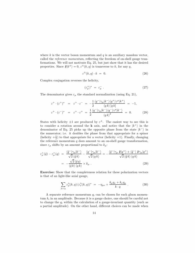
where k is the vector boson momentum and q is an auxiliary massless vector,called the reference momentum, reflecting the freedom of on-shell gauge tran-formations. We will not motivate Eq. 25, but just show that it has the desiredproperties. Since 6k|k±〉 = 0, ε±(k, q) is transverse to k, for any q,

ε±(k, q) · k = 0. (26)

Complex conjugation reverses the helicity,

(ε+µ )∗ = ε−µ . (27)

The denominator gives εµ the standard normalization (using Eq. 21),

ε+ · (ε+)∗ = ε+ · ε− = −1

2

〈q−|γµ|k−〉〈q+|γµ|k+〉〈q k〉 [q k]

= −1,

ε+ · (ε−)∗ = ε+ · ε+ =1

2

〈q−|γµ|k−〉〈q−|γµ|k−〉〈q k〉2

= 0. (28)

States with helicity ±1 are produced by ε±. The easiest way to see this isto consider a rotation around the k axis, and notice that the |k+〉 in thedenominator of Eq. 25 picks up the opposite phase from the state |k−〉 inthe numerator; i.e. it doubles the phase from that appropriate for a spinor(helicity + 1

2 ) to that appropriate for a vector (helicity +1). Finally, changingthe reference momentum q does amount to an on-shell gauge transformation,since εµ shifts by an amount proportional to kµ:

ε+µ (q) − ε+

µ (q) =〈q−|γµ|k−〉√

2 〈q k〉− 〈q−|γµ|k−〉√

2 〈q k〉= −〈q−|γµ 6k|q+〉 + 〈q−| 6kγµ|q+〉√

2 〈q k〉 〈q k〉

= −√

2 〈q q〉〈q k〉 〈q k〉 × kµ . (29)

Exercise: Show that the completeness relation for these polarization vectorsis that of an light-like axial gauge,

∑

λ=±ελ

µ(k, q) (ελν (k, q))∗ = −ηµν +

kµqν + kνqµ

k · q . (30)

A separate reference momentum qi can be chosen for each gluon momen-tum ki in an amplitude. Because it is a gauge choice, one should be careful notto change the qi within the calculation of a gauge-invariant quantity (such asa partial amplitude). On the other hand, different choices can be made when

14

calculating different gauge-invariant quantities. A judicious choice of the qi

can simplify a calculation substantially, by making many terms and diagramsvanish, due primarily to the following identities, where ε±i (q) ≡ ε±(ki, qi = q):

ε±i (q) · q = 0, (31)

ε+i (q) · ε+

j (q) = ε−i (q) · ε−j (q) = 0, (32)

ε+i (kj) · ε−j (q) = ε+

i (q) · ε−j (ki) = 0, (33)

6ε+i (kj)|j+〉 = 6ε−i (kj)|j−〉 = 0, (34)

〈j+| 6ε−i (kj) = 〈j−| 6ε+i (kj) = 0. (35)

In particular, it is useful to choose the reference momenta of like-helicity gluonsto be identical, and to equal the external momentum of one of the opposite-helicity set of gluons.

We can now express any amplitude with massless external fermions andvector bosons in terms of spinor products. Since these products are defined forboth positive- and negative-energy four-momenta, we can use crossing sym-metry to extract a number of scattering amplitudes from the same expression,by exchanging which momenta are outgoing and which incoming. However,because the helicity of a positive-energy (negative-energy) massless spinor hasthe same (opposite) sign as its chirality, the helicities assigned to the parti-cles — bosons as well as fermions — depend on whether they are incoming oroutgoing. Our convention is to label particles with their helicity when theyare considered outgoing (positive-energy); if they are incoming the helicity isreversed.

The spinor-product representation of an amplitude can be related to amore conventional one in terms of Lorentz-invariant objects, the momentuminvariants ki · kj and contractions of the Levi-Civita tensor εµνσρ with exter-nal momenta. The spinor products carry around a number of phases. Someof the phases are unphysical because they are associated with external-stateconventions, such as the definitions of the spinors |i±〉. Physical quantitiessuch as cross-sections (or amplitudes from which an overall phase has beenremoved), when constructed out of the spinor products, will be independentof such choices. Thus for each external momentum label i, if the product 〈i j〉appears then its phase should be compensated by some [i k] (or equivalently1/ 〈i k〉 = − [i k] /sik). If a spinor string appears in a physical quantity, then itmust terminate, i.e. it has the form

〈i1 i2〉 [i2 i3] 〈i3 i4〉 · · · [i2m i1] , (36)

for some m. Multiplying Eq. 36 by 1 = [i4 i1] 〈i1 i4〉 /si1i4 , etc., we can breakup any spinor string into strings of length two and four; the former are just

15

sij ’s (Eq. 18), while the latter can then be evaluated by performing the Diractrace:

〈i j〉 [j l] 〈l m〉 [m i] = tr(

12 (1 − γ5) 6ki 6kj 6kl 6km

)

=1

2

[

sijslm − silsjm + simsjl − 4iε(i, j, l, m)

]

, (37)

where ε(i, j, l, m) = εµνσρkµi kν

j kρl kσ

m. Thus the Levi-Civita contractions are al-ways accompanied by an i and account for the physical phases. In practice, thespinor products offer the most compact representation of helicity amplitudes,but it is useful to know the connection to a more conventional representation.Exercise: Verify the Schouten identity, Eq. 23, by multiplying both sides by[j k] [l i] and using Eq. 37 to simplify.

3 Tree-level techniques

Now we are ready to attack some tree amplitudes, beginning with direct calcu-lation of some simple examples, followed by a discussion of recursive techniquesfor generating more complicated amplitudes, and of the role of supersymmetryand factorization properties in tree-level QCD.

3.1 Simple examples

Let’s first compute the four-gluon tree helicity amplitude Atree4 (1+, 2+, 3+, 4+).a

Since all the gluons have the same helicity, if we choose all the reference mo-menta to be the same null-vector q we can make all the ε+

i · ε+j terms vanish

according to Eq. 32. We can’t choose q to equal one of the external momenta,because that polarization vector would have a singular denominator. But wecould choose for example the null-vector qµ = −2s23k

µ1 +(s12−s23)(2kµ

2 +kµ3 ).

Actually we won’t need the explicit expression for q here, because when westart to evaluate the various diagrams, we find that they always contain atleast one εi · εj , and therefore every diagram in this helicity amplitude van-ishes identically!

This result generalizes easily to more external gluons. Each nonabelianvertex can contribute at most one momentum vector ki to the numerator al-gebra of the graph, and there are at most n − 2 vertices. Thus there are at

aAlthough we will refer to the gluons as all having the same positive helicity, rememberthat the helicity of the two incoming gluons (whichever two they may be) is actually negative.Hence this scattering process changes the helicity of the gluons by the maximum possible,−2 → +2.

16

most n − 2 momentum vectors available to contract with the n polarizationvectors εi (the amplitude is linear in each εi). This means there must be atleast one εi · εj contraction, and so the tree amplitude must vanish wheneverwe can arrange that all the εi · εj vanish. Obviously this can be arranged forthe n-gluon amplitudes with all helicities the same, Atree

n (1+, 2+, 3+, . . . , n+),by again taking all the reference momenta to be identical. And it can be ar-ranged for Atree

n (1−, 2+, 3+, . . . , n+) by the reference momentum choice q2 =q3 = · · · = qn = k1, q1 = kn. Thus we have already computed a large numberof (zero) amplitudes,

Atreen (1±, 2+, 3+, . . . , n+) = 0. (38)

Exercise: Use an analogous argument to show that the following qqgg . . . ghelicity amplitudes also vanish:

Atreen (1−q , 2+

q , 3+, 4+, . . . , n+) = 0. (39)

We’ll see later that an “effective” supersymmetry14 of tree-level QCD is re-sponsible for all these vanishings.

Next we turn to the (nonzero) helicity amplitude Atree4 (1−, 2−, 3+, 4+),

choosing the reference momenta q1 = q2 = k4, q3 = q4 = k1, so that only thecontraction ε−2 · ε+

3 is nonzero. It is easy to see from the color-ordered rules inFig. 5 that only one of the three potential graphs contributes, the one with agluon exchange in the s12 channel. We get

Atree4 (1−, 2−, 3+, 4+)

=

(

i√2

)2 ( −i

s12

)

×[

ε−1 · ε−2 (k1 − k2)µ + (ε−2 )µε−1 · (2k2 + k1) + (ε−1 )µε−2 · (−2k1 − k2)

]

×[

ε+3 · ε+

4 (k3 − k4)µ + (ε+4 )µε+

3 · (2k4 + k3) + (ε+3 )µε+

4 · (−2k3 − k4)]

= − 2i

s12

(

ε−2 · ε+3

)(

ε−1 · k2

)(

ε+4 · k3

)

= − 2i

s12

(

−2

2

[4 3] 〈1 2〉[4 2] 〈1 3〉

) (

− [4 2] 〈2 1〉√2 [4 1]

) (

+〈1 3〉 [3 4]√

2 〈1 4〉

)

= −i〈1 2〉 [3 4]

2

[1 2] 〈1 4〉 [1 4]. (40)

We can pretty up the answer a bit, using antisymmetry (Eq. 20), momentumconservation (Eq. 24), and s34 = s12,

Atree4 (1−, 2−, 3+, 4+) = −i

〈1 2〉 (〈2 3〉 [3 4])([3 4] 〈3 4〉)[1 2] 〈2 3〉 〈3 4〉 〈1 4〉 [1 4]

17

= i〈1 2〉 (−〈2 1〉 [1 4])([1 2] 〈1 2〉)

[1 2] 〈2 3〉 〈3 4〉 〈4 1〉 [1 4]

= i〈1 2〉3

〈2 3〉 〈3 4〉 〈4 1〉 , (41)

or

Atree4 (1−, 2−, 3+, 4+) = i

〈1 2〉4〈1 2〉 〈2 3〉 〈3 4〉 〈4 1〉 . (42)

The remaining four-gluon helicity amplitude can be obtained from thedecoupling identity, Eq. 8:

Atree4 (1−, 2+, 3−, 4+) = −Atree

4 (1−, 3−, 2+, 4+) − Atree4 (1−, 3−, 4+, 2+)

= −i

[

〈1 3〉3〈3 2〉 〈2 4〉 〈4 1〉 +

〈1 3〉3〈3 4〉 〈4 2〉 〈2 1〉

]

= i〈1 3〉3(〈1 2〉 〈3 4〉+ 〈1 4〉 〈2 3〉)

〈1 2〉 〈2 3〉 〈3 4〉 〈4 1〉 〈2 4〉 , (43)

or using the Schouten identity, Eq. 23,

Atree4 (1−, 2+, 3−, 4+) = i

〈1 3〉4〈1 2〉 〈2 3〉 〈3 4〉 〈4 1〉 . (44)

There are no other four-gluon amplitudes to compute, because parity allowsone to reverse all helicities simultaneously, by exchanging 〈 〉 ↔ [ ] and multi-plying by −1 if there are an odd number of gluons.

Note also that the antisymmetry of the color-ordered rules implies thatthe partial amplitudes (even with external quarks) obey a reflection identity,

Atreen (1, 2, . . . , n) = (−1)n Atree

n (n, . . . , 2, 1). (45)

To obtain the unpolarized, color-summed cross-section for four-gluon scat-tering, we insert the nonvanishing helicity amplitudes, Eqs. 42 and 44, intoEq. 10, and sum over the negative helicity gluons i, j:

∑

colorshelicities

[Atree ∗4 Atree

4 ] = g4 N2c (N2

c − 1)4

∑

i>j=1

∑

σ∈S3

(sij)4

sσ(1)σ(2)sσ(2)σ(3)sσ(3)4s4σ(1).

(46)

Of course polarized cross-sections can be constructed just as easily from thehelicity amplitudes.

18

Figure 6: The two nonvanishing graphs in the qqggg helicity amplitude calculation.

Next we calculate a sample five-parton tree amplitude, for two quarks andthree gluons, Atree

5 (1−q , 2+q , 3−, 4+, 5+), where the momenta without subscripts

label the gluons. We choose the gluon reference momenta as q3 = k2, q4 =q5 = k1, so we can use the vanishing relations, Eqs. 34 and 35,

〈2+| 6ε−3 = 6ε+4 |1+〉 = 6ε+

5 |1+〉 = 0. (47)

This kills the graphs where gluons 3 and 5 attach directly to the fermion line,and the graph with a four-gluon vertex, leaving only the two graphs shown inFig. 6.

Graph 1 evaluates to

− i√2

〈2+|(6k3− 6k4− 6k5)|1+〉s12s45

(ε−3 · ε+5 ε+

4 · k5 − ε−3 · ε+4 ε+

5 · k4)

= −i[2 3] 〈3 1〉s12s45

[

− [2 5] 〈1 3〉[2 3] 〈1 5〉

〈1 5〉 [5 4]

〈1 4〉 +[2 4] 〈1 3〉[2 3] 〈1 4〉

〈1 4〉 [4 5]

〈1 5〉

]

= +i[2 3] 〈1 3〉2 [4 5]

s12s45 [2 3] 〈1 4〉 〈1 5〉[

−〈1 5〉 [5 2] − 〈1 4〉 [4 2]]

= −i[2 3] 〈1 3〉3 [4 5]

s12s45 〈1 4〉 〈1 5〉 . (48)

Graph 2 requires a few more uses of the spinor product identities (exercise):

− i√2s12s34

[

〈2+|(6k3+ 6k4− 6k5)|1+〉(

12ε−3 · ε+

4 ε+5 · (k3 − k4) − ε−3 · ε+

5 ε+4 · k3

)

19

−〈2+|(6k3− 6k4)|1+〉ε−3 · ε+4 ε+

5 · (k3 + k4)]

= · · · = +i[2 5] 〈1 3〉3 [3 4]

s12s34 〈1 4〉 〈1 5〉 . (49)

The sum is

Atree5 (1−q , 2+

q , 3−, 4+, 5+) = −i〈1 3〉3 (− [2 3] 〈3 4〉 − [2 5] 〈5 4〉)

s12 〈1 4〉 〈1 5〉 〈3 4〉 〈4 5〉 , (50)

or

Atree5 (1−q , 2+

q , 3−, 4+, 5+) = i〈1 3〉3 〈2 3〉

〈1 2〉 〈2 3〉 〈3 4〉 〈4 5〉 〈5 1〉 . (51)

Once again the expression collapses to a single term.b Spurious singulari-ties associated with the reference momentum choice — such as 1/ 〈1 4〉 in theabove example — are present in individual graphs but cancel out in the gauge-invariant sum.

3.2 Recursive Techniques

By now you can see that color-ordering, plus the spinor helicity formalism, canvastly reduce the number of diagrams, and terms per diagram, that have to beevaluated. However, with more external legs the results still get more complexand difficult to carry out by hand. Fortunately, a technique is available forgenerating tree amplitudes recursively in the number of legs.15 Even if onecannot simplify analytically the expressions obtained in this way, the recursiveapproach lends itself to efficient numerical evaluation.

In order to get a tree-level recursion relation, we need to construct anauxiliary quantity with one leg off-shell. For the construction of pure-glueamplitudes, we define the off-shell current Jµ(1, 2, . . . , n) to be the sum ofcolor-ordered (n+1)-point Feynman graphs, where legs 1, 2, . . . , n are on-shellgluons, and leg “µ” is off-shell, as shown in Fig. 7. The uncontracted vectorindex on the off-shell leg is also denoted by µ; the off-shell propagator is definedto be included in Jµ. Since Jµ is an off-shell quantity, it is gauge-dependent.For example, Jµ depends on the reference momenta for the on-shell gluons,which must therefore be kept fixed until after one has extracted an on-shellresult. One can also construct amplitudes with external quarks recursively, byintroducing an off-shell quark current15 as well as the gluon current Jµ, butwe will not do so here.

bWe have multiplied both graphs here by (−1); this external state convention makesthe qqggg partial amplitudes equal to the gluino partial amplitudes ggggg, so that thesupersymmetry Ward identities below can be applied without extra minus signs.

20

Figure 7: The off-shell gluon current Jµ(1, 2, . . . , n). Leg “µ” is the only off-shell leg.

It is easy to write down a recursion relation for Jµ, by following the off-shell line back into the diagram. One first encounters either a three-gluonvertex or a four-gluon vertex. Each of the off-shell lines branching out fromthis vertex attaches to a smaller number of on-shell gluons, thus we have therecursion relation15 depicted in Fig. 8,

Jµ(1, . . . , n) =−i

P 21,n

[

n−1∑

i=1

V µνρ3 (P1,i, Pi+1,n) Jν(1, . . . , i) Jρ(i + 1, . . . , n)

+

n−1∑

j=i+1

n−2∑

i=1

V µνρσ4 Jν(1, . . . , i) Jρ(i + 1, . . . , j) Jσ(j + 1, . . . , n)

]

,

(52)

where the Vi are just the color-ordered gluon self-interactions,

V µνρ3 (P, Q) =

i√2

(ηνρ(P − Q)µ + 2ηρµQν − 2ηµνP ρ) ,

V µνρσ4 =

i

2(2ηµρηνσ − ηµνηρσ − ηµσηνρ) , (53)

andPi,j ≡ ki + ki+1 + · · · + kj . (54)

The Jµ satisfy the photon decoupling relation,

Jµ(1, 2, 3, . . . , n) + Jµ(2, 1, 3, . . . , n) + · · · + Jµ(2, 3, . . . , n, 1) = 0, (55)

the reflection identity

Jµ(1, 2, 3, . . . , n) = (−1)n+1 Jµ(n, . . . , 3, 2, 1), (56)

21

Figure 8: The recursion relation for the off-shell gluon current Jµ(1, 2, . . . , n).

and current conservation,

Pµ1,n Jµ(1, 2, . . . , n) = 0. (57)

In some cases, the recursion relations can be solved in closed form.15,16 Thesimplest case is (as expected) when all on-shell gluons have the same helicity,for which we choose the common reference momentum q, and then

Jµ(1+, 2+, . . . , n+) =〈q−|γµ 6P 1,n|q+〉√

2 〈q 1〉 〈1 2〉 · · · 〈n − 1, n〉 〈n q〉. (58)

Let’s verify that this expression solves Eq. 52. Note first that the V4 term doesnot contribute at all, nor the first term in V3, because after Fierzing we get afactor of 〈q q〉 = 0. Thus the right-hand side of Eq. 52 becomes (using 〈q q〉 = 0to commute and rearrange terms)

1√2P 2

1,n 〈q 1〉 〈1 2〉 · · · 〈n − 1, n〉 〈n q〉

n−1∑

i=1

〈i, i + 1〉〈i q〉 〈q, i + 1〉

×(

〈q−|γµ 6P i+1,n|q+〉〈q−| 6P i+1,n 6P 1,i|q+〉

−〈q−|γµ 6P 1,i|q+〉〈q−| 6P 1,i 6P i+1,n|q+〉)

=〈q−|γµ 6P 1,n|q+〉√

2P 21,n 〈q 1〉 〈1 2〉 · · · 〈n − 1, n〉 〈n q〉

×[

n−1∑

i=1

〈i, i + 1〉〈i q〉 〈q, i + 1〉 〈q

−| 6P i+1,n

]

6P 1,n|q+〉 . (59)

22

Using the identity

n−1∑

i=1

〈i, i + 1〉〈i q〉 〈q, i + 1〉 〈q

−| 6P i+1,n =〈1−| 6P 1,n

〈1 q〉 , (60)

we get the desired result, Eq. 58.Exercise: Prove the identity, Eq. 60, by first proving the identity

k−1∑

i=j

〈i, i + 1〉〈i q〉 〈q, i + 1〉 =

〈j k〉〈j q〉 〈q k〉 . (61)

The “eikonal” identity, Eq. 61, also plays a role in understanding the structureof the soft singularities of QED amplitudes, when these are obtained from QCDpartial amplitudes by the replacement T a → 1 (see Sections 3.4 and 3.5).

The current where the first on-shell gluon has negative helicity can beobtained similarly,

Jµ(1−, 2+, . . . , n+) =〈1−|γµ 6P 2,n|1+〉√

2 〈1 2〉 · · · 〈n 1〉

n∑

m=3

〈1−| 6km 6P 1,m|1+〉P 2

1,m−1P21,m

, (62)

where the reference momentum choice is q1 = k2, q2 = · · · = qn = k1.Exercise: Show this.

Amplitudes with (n+1) legs are obtained from the currents Jµ(1, 2, . . . , n)by amputating the off-shell propagator (multiplying by i P 2

1,n), contracting theµ index with the appropriate on-shell polarization vector εµ

n+1, and takingP 2

1,n = k2n+1 → 0. In the case of Jµ(1+, 2+, . . . , n+), there is no P 2

1,n polein the current, so the amplitude must vanish for both helicities of gluon (n +1), in accord with Eq. 38. In the case of Jµ(1−, 2+, . . . , n+), the pole termrequirement picks out the term m = n in Eq. 62. Using reference momentumqn+1 = kn for ε−n+1, we obtain (replacing 6P 1,n → − 6kn+1, etc.),

Atreen+1(1

−, 2+, . . . , n+, (n + 1)−)

= −i〈n+|γµ|(n + 1)+〉√

2 [n, n + 1]

〈1−|γµ 6P 1,n|1+〉√2 〈1 2〉 · · · 〈n 1〉

〈1−| 6kn 6P 1,n|1+〉P 2

1,n−1

= −i〈1, n + 1〉

〈1 2〉 · · · 〈n 1〉〈n + 1, 1〉 〈1 n〉 [n, n + 1] 〈n + 1, 1〉

sn,n+1, (63)

or

Atreen (1−, 2−, 3+, 4+, . . . , n+) = i

〈1 2〉4〈1 2〉 · · · 〈n 1〉 . (64)

23

Applying the decoupling identity, Eq. 8, and the spinor identity, Eq. 61, itis easy to obtain the remaining maximally helicity violating (MHV) or Parke-Taylor17 helicity amplitudes,

Atree MHVjk ≡ Atree

n (1+, . . . , j−, . . . , k−, . . . , n+) = i〈j k〉4

〈1 2〉 · · · 〈n 1〉 . (65)

These remarkably simple amplitudes were first conjectured by Parke andTaylor17 on the basis of their collinear limits (see below) and photon decouplingrelations, and were rigorously proven correct by Berends and Giele15 usingthe above recursive approach. The other nonvanishing helicity configurations(beginning at n = 6) are typically more complicated. The MHV amplitudescan be used as the basis of approximation schemes, however.18

3.3 Supersymmetry

What does supersymmetry have to do with a non-supersymmetric theory suchas QCD? The answer is that tree-level QCD is “effectively” supersymmetric,14

and the “non-supersymmetry” only leaks in at the loop level. To see thesupersymmetry of an n-gluon tree amplitude is simple: It has no loops in it,so it has no fermion loops in it. Therefore the fermions in the theory might aswell be gluinos, i.e. at tree-level the theory might as well be super Yang-Millstheory. Tree amplitudes with quarks are also supersymmetric, but at the levelof partial amplitudes: after the color information has been stripped off, thereis nothing to distinguish a quark from a gluino. Supersymmetry leads to extrarelations between amplitudes, supersymmetric Ward identities (SWI),19 whichcan be quite useful in saving computational labor.14

To derive supersymmetric Ward identities,19,3 we use the fact that thesupercharge Q annihilates the vacuum (we are considering exactly supersym-metric theories, not spontaneously or softly broken ones!),

0 = 〈0|[Q, Φ1Φ2 · · ·Φn]|0〉 =

n∑

i=1

〈0|Φ1 · · · [Q, Φi] · · ·Φn|0〉 . (66)

When the fields Φi create helicity eigenstates, many of the [Q, Φi] terms canbe arranged to vanish. To proceed, we need the precise commutation relationsof the supercharge with the fields g±(k), Λ±(k), which create gluon and gluinostates of momentum k (k2 = 0) and helicity ±. We multiply Q by a Grassmannspinor parameter η, defining Q(η) ≡ ηαQα, so that Q(η) commutes with theFermi fields as well as the Bose fields. The commutators have the form

[

Q(η), g±(k)]

= ∓Γ±(k, η) Λ±(k),

24

[

Q(η), Λ±(k)]

= ∓Γ∓(k, η) g±(k), (67)

where Γ(k, η) is linear in η, and has its form constrained by the Jacobi identityfor the supersymmetry algebra,

0 = [[Q(η), Q(ζ)] , Φ(k)] + [[Q(ζ), Φ(k)] , Q(η)] + [[Φ(k), Q(η)] , Q(ζ)] , (68)

where Φ(k) is either g±(k) or Λ±(k). Since [Q(η), Q(ζ)] = −2iη 6Pζ, we need

Γ+(k, η)Γ−(k, ζ) + Γ−(k, η)Γ+(k, ζ) = −2iη 6kζ. (69)

A solution to Eq. 69, which also has the correct behavior under rotationsaround the k axis, is (cf. Eq. 19)

Γ+(k, η) = ηu−(k), Γ−(k, η) = ηu+(k) = u−(k)η. (70)

Finally, we choose η to be a Grassmann parameter θ, multiplied by the spinorfor an arbitrary massless vector q, and choose q so as to simplify the identities(much like the choice of reference momentum in εµ

±(q)). Then Γ±(k, η) become

Γ+(k, q) = θ 〈q+|k−〉 = θ [q k] , Γ−(k, q) = θ 〈q−|k+〉 = θ 〈q k〉 . (71)

The simplest case is the like-helicity one. We start with

0 =⟨

0|[Q(η(q)), Λ+1 g+

2 g+3 · · · g+

n ]|0⟩

= −Γ−(k1, q)An(g+1 , g+

2 , . . . , g+n ) + Γ+(k2, q)An(Λ+

1 , Λ+2 , g+

3 , . . . , g+n )

+ · · ·+ Γ+(kn, q)An(Λ+1 , g+

2 , . . . , g+n−1, Λ

+n ). (72)

Since massless gluinos, like quarks, have only helicity-conserving interactionsin (super) QCD, all of the amplitudes but the first in Eq. 72 must vanish.Therefore so must the like-helicity amplitude An(g+

1 , g+2 , . . . , g+

n ). Similarly,with one negative helicity we get

0 =⟨

0|[Q(η(q)), Λ+1 g−2 g+

3 · · · g+n ]|0

⟩

= −Γ−(k1, q)An(g+1 , g−2 , g+

3 , . . . , g+n ) − Γ−(k2, q)An(Λ+

1 , Λ−2 , g+

3 , . . . , g+n ),

(73)

where we have omitted the vanishing fermion-helicity-violating amplitudes.Now we use the freedom to choose q, setting q = k1 to show the secondamplitude vanishes and setting q = k2 to show the first vanishes. Thus wehave recovered Eqs. 38 and 39.

25

With two negative helicities, we begin to relate nonzero amplitudes:

0 =⟨

0|[Q(η(q)), g−1 g−2 Λ+3 g+

4 · · · g+n ]|0

⟩

= Γ−(k1, q)An(Λ−1 , g−2 , Λ+

3 , . . . , g+n ) + Γ−(k2, q)An(g−1 , Λ−

2 , Λ+3 , . . . , g+

n )

−Γ−(k3, q)An(g−1 , g−2 , g+3 , . . . , g+

n ). (74)

Choosing q = k1, we get

An(g−1 , g−2 , g+3 , g+

4 , . . . , g+n ) =

〈1 2〉〈1 3〉 × An(g−1 , Λ−

2 , Λ+3 , g+

4 , . . . , g+n ). (75)

No perturbative approximations were made in deriving any of the aboveSWI; thus they hold order-by-order in the loop expansion. They apply directlyto QCD tree amplitudes, because of their “effective” supersymmetry. Butthey can also be used to save some work at the loop level (see below). Sincesupersymmetry commutes with color, the SWI apply to each color-orderedpartial amplitude separately. Summarizing the above “MHV” results (andsimilar ones including a pair of external scalar fields), we have

ASUSYn (1±, 2+, 3+, . . . , n+) = 0, (76)

ASUSYn (1−, 2−P , 3+

P , 4+, . . . , n+) =

( 〈1 2〉〈1 3〉

)2|hP |ASUSY

n (1−, 2−φ , 3+φ , 4+, . . . , n+).

(77)

Here no subscript refers to a gluon, while φ refers to a scalar particle (forwhich the “helicity” ± means particle vs. antiparticle), and P refers to ascalar, fermion or gluon, with respective helicity hP = 0, 1

2 , 1.We can use Eq. 77 at the four-point level to obtain the qqgg amplitudes

from the four-gluon ones, Eqs. 42 and 44:

Atree4 (1−q , 2+

q , 3−, 4+) = i〈1 3〉3 〈2 3〉

〈1 2〉 〈2 3〉 〈3 4〉 〈4 1〉 ,

Atree4 (1−q , 2+

q , 3+, 4−) = i〈1 4〉3 〈2 4〉

〈1 2〉 〈2 3〉 〈3 4〉 〈4 1〉 . (78)

Exercise: Check the SWI at the five-point level, comparing the qqggg ampli-tude, Eq. 51, and the ggggg amplitude from Eq. 65.

3.4 Factorization Properties

Analytic properties of amplitudes are very useful as consistency checks of thecorrectness of a calculation, but they can also sometimes be used to help con-struct amplitudes. At tree-level, the principal analytic property is the pole

26

behavior as kinematic invariants vanish, due to an almost on-shell interme-diate particle. As mentioned above, color-ordered amplitudes can only havepoles in channels corresponding to the sum of a sum of cyclically adjacent mo-menta, i.e. as P 2

i,j → 0, where Pµi,j ≡ (ki + ki+1 + · · · + kj)

µ. This is becausesingularities arise from propagators going on-shell, and propagators for color-ordered graphs always carry momenta of the form Pµ

i,j . We refer to channelsformed by three or more adjacent momenta as multi-particle channels, and thetwo-particle channels as collinear channels.

In a multi-particle channel, a true pole can develop as P 21,m → 0,

Atreen (1, . . . , n) ∼

∑

λ

Atreem+1(1, . . . , m, Pλ)

i

P 21,m

Atreen−m+1(m + 1, . . . , n, P−λ),

(79)where P1,m is the intermediate momentum and λ denotes the helicity of theintermediate state P . Our outgoing-particle helicity convention means thatthe intermediate helicity is reversed in going from one product amplitude tothe other.

Most multi-parton amplitudes have multi-particle poles, but the MHVtree amplitudes do not, due to the vanishing of Atree

n (1±, 2+, . . . , n+). Whenwe attempt to factorize an MHV amplitude on a multi-particle pole, as inFig. 9(a), we have only three negative helicities (one from the intermediategluon) to distribute among the two product amplitudes. Therefore one of thetwo must vanish, so the pole cannot be present. Thus the vanishing SWI alsoguarantees the simple structure of the nonvanishing MHV tree amplitudes:only collinear (two-particle) singularities of adjacent particles are permitted.

An angular momentum obstruction suppresses collinear singularities inQCD amplitudes. For example, a helicity +1 gluon cannot split into two pre-cisely collinear helicity ±1 gluons and still conserve angular momentum alongthe direction of motion. Nor can it split into a + 1

2 fermion and − 12 antifermion.

The 1/si,i+1 from the propagator is cancelled by numerator factors, down tothe square-root of a pole, 1√

si,i+1∼ 1

〈i, i+1〉 ∼ 1[i, i+1] . Thus the spinor products,

square roots of Lorentz invariants, are ideal for capturing the collinear behav-ior in QCD. The general form of the collinear singularities for tree amplitudesis shown in Fig. 9(b),

Atreen (. . . , aλa , bλb , . . .)

a‖b−→∑

λ=±Splittree−λ (z, aλa , bλb)Atree

n−1(. . . , Pλ, . . .) , (80)

where Splittree denotes a splitting amplitude, the intermediate state P hasmomentum kP = ka + kb and helicity λ, and z describes the longitudinal mo-mentum sharing, ka ≈ zkP , kb ≈ (1 − z)kP . Universality of the multi-particle

27

Figure 9: (a) Factorization of an MHV tree amplitude on a multi-particle pole — one of thetwo product amplitudes always vanishes. (b) General behavior of a tree-level amplitude inthe collinear limit where ka is parallel to kb; S stands for the splitting amplitude Splittree.

and collinear factorization limits can be derived in field theory,20 or perhapsmore elegantly in string theory,3 which lumps all the field theory diagrams oneach side of the pole into one string diagram.

An easy way to extract the splitting amplitudes Splittree in Eq. 80 isfrom the collinear limits of five-point amplitudes. For example, the limit ofAtree

5 (1−, 2−, 3+, 4+, 5+) as k4 and k5 become parallel determines the gluonsplitting amplitude Splittree− (a+, b+):

Atree5 (1−, 2−, 3+, 4+, 5+) = i

〈1 2〉4〈1 2〉 〈2 3〉 〈3 4〉 〈4 5〉 〈5 1〉

4‖5−→

1√

z(1 − z) 〈4 5〉× i

〈1 2〉4〈1 2〉 〈2 3〉 〈3 P 〉 〈P 1〉

= Splittree− (4+, 5+) × Atree4 (1−, 2−, 3+, P+).

(81)

Using also the 2 ‖ 3 and 5 ‖ 1 limits, plus parity, we can infer the full set ofg → gg splitting amplitudes17,21,15,3

Splittree− (a−, b−) = 0,

Splittree− (a+, b+) =1

√

z(1 − z) 〈a b〉,

28

Splittree+ (a+, b−) =(1 − z)2

√

z(1 − z) 〈a b〉,

Splittree− (a+, b−) = − z2

√

z(1 − z) [a b]. (82)

The g → qq and q → qg splitting amplitudes are also easy to obtain, from thelimits of Eq. 51, etc.

Since the collinear limits of QCD amplitudes are responsible for partonevolution, it is not surprising that the residue of the collinear pole in thesquare of a splitting amplitude gives the (color-stripped) polarized Altarelli-Parisi splitting probability.22

Exercise: Show that the unpolarized g → gg splitting probability, from sum-ming over the terms in Eq. 82, has the familiar form

Pgg(z) ∝ 1 + z4 + (1 − z)4

z(1 − z), (83)

neglecting the plus prescription and δ(1 − z) term.QCD amplitudes also have universal behavior in the soft limit, where all

components of a gluon momentum vector ks go to zero. At tree level one finds

Atreen (. . . , a, s, b, . . .)

ks→0−→ Softtree(a, s, b)Atreen−1(. . . , a, b, . . .). (84)

The soft or “eikonal” factor,

Softtree(a, s, b) =〈a b〉

〈a s〉 〈s b〉 , (85)

depends on both color-ordered neighbors of the soft gluon s, because the setsof graphs where s is radiated from legs a and b are both singular in the softlimit. On the other hand, the soft behavior is independent of both the identity(gluon vs. quark) and the helicity of partons a and b, reflecting the classicalorigin of soft radiation. (See George Sterman’s lectures in this volume for adeeper and more general discussion.23)Exercise: Verify the soft behavior, Eq. 84, for any of the above multipartontree amplitudes.

As Zoltan Kunszt will explain in more detail,2 the universal soft andcollinear behavior of tree amplitudes, and therefore of tree-level cross-sections,makes possible general procedures for isolating the infrared divergences in thereal, bremsstrahlung contribution to an arbitrary NLO cross-section, and can-celling these divergences against corresponding ones in one-loop amplitudes.

29

But the factorization limits also strongly constrain the form of tree and loopamplitudes. It is quite possible that they uniquely determine a rational func-tion of the n-point variables for n ≥ 6, given the lower-point amplitudes, butthis has not yet been proven.Exercise: Show that

ε(1, 2, 3, 4)

〈1 2〉 〈2 3〉 〈3 4〉 〈4 5〉 〈5 1〉 (86)

provides a counterexample to the uniqueness assertion at the five-point level,because it is nonzero, yet has nonsingular collinear limits in all channels.

3.5 Beyond QCD (briefly)

This school is titled “QCD and Beyond”, so let me indicate briefly how thetechniques discussed here can be applied beyond pure QCD. Consider ampli-tudes containing a single external electroweak vector boson, W , Z or γ. Interms of U(Nc) = SU(Nc) × U(1) group theory, the electroweak boson gener-ator corresponds to the U(1) generator, proportional to the identity matrix.Thus the color decomposition is identical to that obtained by ignoring the weakboson. For example, the tree amplitudes qqg · · · gγ can be written as

Atree,1γn (1q, 2q, 3, . . . , n − 1, nγ) =

√2Qqeg

n−3∑

σ∈Sn−3

(T aσ(3) · · ·T aσ(n−1))ı2

i1

×Atree,1γn (1q, 2q; σ(3), . . . , σ(n − 1); nγ), (87)

where Qq is the quark charge. Furthermore, the partial amplitudes Atree,1γn can

be obtained for free from the partial amplitudes Atreen for qqg · · · g. One simply

inserts T an = 1 in the color decomposition for Atreen , Eq. 5, and matches the

color structures with Eq. 87. The result is3

Atree,1γn (1q, 2q; 3, . . . , n − 1; nγ) = Atree

n (1q, 2q; n, 3, 4, . . . , n − 1))

+Atreen (1q, 2q; 3, n, 4, . . . , n − 1))

+ · · ·+Atreen (1q, 2q; 3, 4, . . . , n − 1, n)) . (88)

Compare this “photon coupling equation” with the photon decoupling equa-tion for pure gluon amplitudes, Eq. 8. When more quark lines are present,one has to pay attention to the −1/Nc terms mentioned in Section 2.1, sincethese distinguish SU(Nc) from U(1); however, similar formulas can be derived,including also multiple photon emission.10,24,25

The emission of a massive vector particle — a W , Z or virtual photon —would seem to require an extension of the helicity formalism of Section 2.2.

30

However, in most cases one is actually interested in processes where the vectorboson “decays” to a pair of massless fermions. (One or more of these fermionsmay be in the initial state.) Then the formalism for massless fermions andvectors can still be applied, albeit with the introduction of one additional (butphysical) four-vector. Thus electroweak processes such as e+e− annihilation tofour fermions may be calculated very efficiently using the helicity formalism.

Massive fermions do require a serious extension of the formalism. It is pos-sible to represent a massive spinor in terms of two massless ones26; alternativelyone can represent massive spinor outer products in terms of “spin vectors”.27

In either case the price is at least one additional four-vector, this time an un-physical one. Not only is the formalism more cumbersome than for masslessfermions, but so are the results. Amplitudes with a helicity flip on the quarkline no longer vanish; nor do those that were protected by a supersymmetryWard identity in the massless case, such as Atree

4 (1q, 2q, 3+, 4+).

4 Loop-level techniques

In order to increase the precision of QCD predictions, we need to go to next-to-leading-order, and in particular, to have efficient techniques for computingthe one-loop amplitudes which now enter. Here the algebra gets considerablymore complicated, even with the use of color-ordering and the helicity for-malism, because there are more off-shell lines, and more nonabelian vertices.Furthermore, one has to evaluate loop integrals with loop momenta inserted inthe numerator; reducing these integrals often requires the inversion of matriceswhich can generate a big mess. Although the helicity and color tools are stillvery useful, we will need additional tools for organizing loop amplitudes inorder to minimize the growth of expressions in intermediate steps.

4.1 Supersymmetry and background-field gauge

At loop level, QCD “knows” it is not supersymmetric. However, one canstill rearrange the sum over internal spins propagating around the loop, inorder to take advantage of supersymmetry. For example, for an amplitudewith all external gluons, and a gluon circulating around the loop, we canuse supersymmetry to trade the internal gluon loop for a scalar loop. Werewrite the internal gluon loop g (and fermion loop f) as a supersymmetriccontribution plus a complex scalar loop s,

g = (g + 4f + 3s) − 4(f + s) + s = AN=4 − 4 AN=1 + Ascalar,

f = (f + s) − s = AN=1 − Ascalar. (89)

31

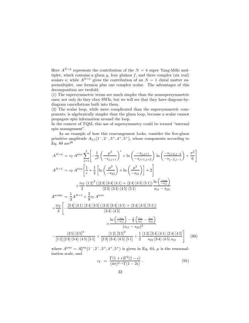
Here AN=4 represents the contribution of the N = 4 super Yang-Mills mul-tiplet, which contains a gluon g, four gluinos f , and three complex (six real)scalars s; while AN=1 gives the contribution of an N = 1 chiral matter su-permultiplet, one fermion plus one complex scalar. The advantages of thisdecomposition are twofold:(1) The supersymmetric terms are much simpler than the nonsupersymmetricones; not only do they obey SWIs, but we will see that they have diagram-by-diagram cancellations built into them.(2) The scalar loop, while more complicated than the supersymmetric com-ponents, is algebraically simpler than the gluon loop, because a scalar cannotpropagate spin information around the loop.In the context of TQM, this use of supersymmetry could be termed “internalspin management”.

As an example of how this rearrangement looks, consider the five-gluonprimitive amplitude A5;1(1

−, 2−, 3+, 4+, 5+), whose components according toEq. 89 are28

AN=4 = cΓ Atree5

∑

j=1

[

− 1

ǫ2

(

µ2

−sj,j+1

)ǫ

+ ln

( −sj,j+1

−sj+1,j+2

)

ln

(−sj+2,j−2

−sj−2,j−1

)

+π2

6

]

AN=1 = cΓ Atree

[

1

ǫ+

1

2

[

ln

(

µ2

−s23

)

+ ln

(

µ2

−s51

)]

+ 2

]

+icΓ

2

〈1 2〉2 (〈2 3〉 [3 4] 〈4 1〉 + 〈2 4〉 [4 5] 〈5 1〉)〈2 3〉 〈3 4〉 〈4 5〉 〈5 1〉

ln(

−s23

−s51

)

s51 − s23

Ascalar =1

3AN=1 +

2

9cΓ Atree

+icΓ

3

[

− [3 4] 〈4 1〉 〈2 4〉 [4 5] (〈2 3〉 [3 4] 〈4 1〉 + 〈2 4〉 [4 5] 〈5 1〉)〈3 4〉 〈4 5〉

×ln

(

−s23

−s51

)

− 12

(

s23

s51− s51

s23

)

(s51 − s23)3

− 〈3 5〉 [3 5]3

[1 2] [2 3] 〈3 4〉 〈4 5〉 [5 1]+

〈1 2〉 [3 5]2

[2 3] 〈3 4〉 〈4 5〉 [5 1]+

1

2

〈1 2〉 [3 4] 〈4 1〉 〈2 4〉 [4 5]

s23 〈3 4〉 〈4 5〉 s51

]

(90)

where Atree = Atree5 (1−, 2−, 3+, 4+, 5+) is given in Eq. 64, µ is the renormal-

ization scale, and

cΓ =Γ(1 + ǫ)Γ2(1 − ǫ)

(4π)2−ǫΓ(1 − 2ǫ). (91)

32

These amplitudes contain both infrared and ultraviolet divergences, which havebeen regulated dimensionally with D = 4− 2ǫ, dropping O(ǫ) corrections. Wesee that the three components have quite different analytic structure, indi-cating that the rearrangement is a natural one. As promised, the N = 4supersymmetric component is the simplest, followed by the N = 1 component.The non-supersymmetric scalar component is the most complicated, yet it isstill simpler than the direct gluon calculation, because it does not mix all threecomponents together.

We can understand why the supersymmetric decomposition works by quan-tizing QCD in a special gauge, background-field gauge.29 The color-orderedrules in Fig. 5 were obtained using the Lorentz gauge condition ∂µAµ = 0,where Aµ ≡ Aa

µT a with T a in the fundamental representation. After perform-ing the Faddeev-Popov trick to integrate over the gauge-fixing condition, oneobtains the additional term in the Lagrangian

− 1

2ξTr(∂µAµ)2, (92)

where we chose the integration weight ξ = 1 (Lorentz-Feynman gauge) inFig. 5. To quantize in background-field gauge one splits the gauge field into aclassical background field and a fluctuating quantum field, Aµ = AB

µ + AQµ ,

and imposes the gauge condition DBµ AQ

µ = 0, where DBµ = ∂µ − i√

2gAB

µ is

the background-field covariant derivative, with ABµ evaluated in the adjoint

representation. Now the Faddeev-Popov integration (for ξ = 1) leads to theadditional term, replacing Eq. 92,

− 1

2Tr(DB

µ AQµ )2 = −1

2Tr(∂µAQ

µ − i√2g[AB

µ , AQµ ])2. (93)

For one-loop calculations we require only the terms in the Lagrangian thatare quadratic in the quantum field AQ

µ ; AQµ describes the gluon propagating

around the loop, while ABµ corresponds to the external gluons. Expanding out

the classical Lagrangian − 14 Tr(F 2

µν) plus Eq. 93, one finds that the three-gluon(QQB) and four-gluon (QQBB) color-ordered vertices are modified from thoseshown in Fig. 5 to

V QQBµνρ =

i√2

[

ηµν(k − p)ρ − 2ηρνqµ + 2ηρµqν

]

V QQBBµνρλ = − i

2

[

ηµνηρλ + 2ηµληνρ − 2ηµρηνλ

]

; (94)

the remaining rules remain the same. In background-field gauge the interac-tions of a scalar and of a ghost with the background field are identical, and

33

are given by

V ssBρ =

i√2(k − p)ρ

V ssBBρλ = − i

2ηρλ ; (95)

of course a ghost loop has an additional overall minus sign.Now let’s use Eqs. 94 and 95 to compare the gluon and scalar contribu-

tions to an n-gluon one-loop amplitude, focusing on the terms with the mostfactors of the loop momentum in the numerator of the Feynman diagrams,because these give rise to the greatest algebraic complications in explicit com-putations (see the next subsection). The loop momentum only appears in thetri-linear vertices, and only in the first term in V QQB

µνρ , because q is an external

momentum. This term matches V ssBρ up to the ηµν factor. Thus the lead-

ing loop-momentum terms for a gluon loop (including the ghost contribution)are identical to those for a complex scalar loop: ηµ

µ − 2 = 2 in D = 4. Indimensional regularization this result is still true if one uses a scheme such asdimensional reduction30 or four-dimensional helicity,5 which leaves the numberof physical gluon helicities fixed at two. In fact, as we’ll see shortly, the differ-ence between a gluon loop and a complex scalar loop has two fewer powers ofthe loop momentum in the numerator — at most m − 2 powers in a diagramwith m propagators in the loop, versus m for the gluon or scalar loop alone.In summary, a gluon loop is a scalar loop “plus a little bit more”.

To treat fermion loops in the same way, it is convenient to use a “second-order formalism” where the propagator looks more like that of a boson.31,32 Itis not necessary to generate the full Feynman rules; it suffices to inspect theeffective action Γ(A), which generates the one-particle irreducible (1PI) graphs.Scattering amplitudes are obtained by attaching tree diagrams to the externallegs of 1PI graphs, but this process does not involve the loop momentum and isidentical for all internal particle contributions. The scalar, fermion and gluoncontributions to the effective action (the latter in background-field gauge andincluding the ghost loop) are

Γscalar(A) = ln det−1[0]

(

D2)

,

Γfermion(A) =1

2ln det

1/2[1/2]

(

D2 − g√2

12σµνFµν

)

,

Γgluon(A) = ln det−1/2[1]

(

D2 − g√2ΣµνFµν

)

+ ln det[0](

D2)

, (96)

where D is the covariant derivative, F is the external field strength, 12σµν (Σµν)

is the spin- 12 (spin-1) Lorentz generator, and det[J] is the one-loop determinant

34

for a particle of spin J in the loop. The fermionic contribution has beenrewritten in second-order form using

ln det1/2[1/2] (6D) =

1

2ln det

1/2[1/2]

(

6D2)

(97)

and6D2 = 1

2{6D, 6D} + 12 [6D, 6D] = D2 − g√

212σµνFµν . (98)

We want to compare the leading behavior of each contribution in Eq. 96for large loop momentum ℓ. The leading behavior possible for an m-point 1PIgraph is ℓm, as we saw above in the gluon and scalar cases. The leading term al-ways comes from the D2 term in Eq. 96, because Fµν contains only the externalmomenta, not the loop momentum. Using Tr[0](1) = 1, Tr[1/2](1) = Tr[1] = 4,we see that the D2 term cancels between the scalar and fermion loop, andbetween the fermion and gluon loop; hence it cancels in any supersymmetriclinear combination. Subleading terms in supersymmetric combinations comefrom using one or more factors of F in generating a graph; each F costs onepower of ℓ. Terms with a lone F cancel, thanks to Trσµν = TrΣµν = 0, so thecancellation for an m-point 1PI graph is from ℓm down to ℓm−2. In a gaugeother than background-field gauge, the cancellations involving the gluon loopwould no longer happen diagram by diagram.Exercise: By comparing the traces of products of two and three σµν ’s (Σµν ’s),show that for AN=4 the cancellation is all the way down to ℓm−4.

The loop-momentum cancellations are responsible for the much simplerstructure of the supersymmetric contributions to A5;1(1

−, 2−, 3+, 4+, 5+) inEq. 90, and similarly for generic n-gluon loop amplitudes. As we sketch in thenext subsection, loop integrals with fewer powers of the loop momentum in thenumerator can be reduced more simply to “scalar” integrals — integrals withno loop momenta in the numerator. In the (supersymmetric) case where them-point 1PI graphs have at most ℓm−2 behavior, the set of integrals obtainedis so restricted that such an amplitude can be reconstructed directly from itsabsorptive parts33 (see Section 4.3).

Similar rearrangements can be carried out for one-loop amplitudes withexternal fermions.33,10 For example, the amplitude with two external quarksand the rest gluons has many diagrams where a fermion goes part of the wayaround the loop, and a gluon the rest of the way around. It is easy to seethat these graphs have an ℓm−1 behavior. If one now subtracts from eachgraph the same graph where a scalar replaces the gluon in the loop, thenthe background-field gauge rules, Eqs. 94 and 95, show that the differenceobeys the “supersymmetric” ℓm−2 criterion (even though in this case it is notsupersymmetric). Subtracting and adding back this scalar contribution is a

35

rearrangement analogous to the n-gluon supersymmetric rearrangement, anddoes aid practical calculations.10

Finally, these rearrangements can be motivated by the Neveu-Schwarz-Ramond representation of superstring theory.4,5,31,9 This representation is notmanifestly space-time supersymmetric, but at one loop it corresponds to fieldtheory in background-field gauge (for 1PI graphs) and to a second-order formal-ism for fermions.31 At tree-level — and at loop-level for the trees that have tobe sewn onto 1PI graphs to construct amplitudes — string theory correspondsto the nonlinear Gervais-Neveu gauge,34,31 ∂µAµ − i√

2gAµAµ = 0. This gauge

choice also simplifies the respective calculations, though we omit the detailshere. String theory may have more to teach us about special gauges at themulti-loop level.

4.2 Loop Integral Reduction

Even if one takes advantage of the various techniques already outlined, loop cal-culations with many external legs can still be very complex. Most of the com-plication arises at the stage of doing the loop integrals. The general one-loopm-point integral in 4 − 2ǫ dimensions (for vanishing internal particle masses)is

Im

[

P (ℓµ)]

=

∫

d4−2ǫℓ

(2π)4−2ǫ

P (ℓµ)

ℓ2(ℓ − k1)2(ℓ − k1 − k2)2 · · · (ℓ − k1 − k2 − · · · − km−1)2

(99)where ki, i = 1, . . . , m, are the momenta flowing out of the loop at leg i,and P (ℓµ) is a polynomial in the loop momentum. As we’ll outline, Eq. 99can be reduced recursively to a linear combination of scalar integrals Im[1],where m = 2, 3, 4. The problem is that for large m the reduction coefficientscan depend on many kinematic variables, and are often unwieldy and containspurious singularities.

Here we illustrate one reduction procedure that works well for large m.35 Ifm ≥ 5, then for generic kinematics we have at least four independent momenta,say p1 = k1, p2 = k1 + k2, p3 = k1 + k2 + k3, p4 = k1 + k2 + k3 + k4. We candefine a set of dual momenta vµ

i ,

vµ1 = ε(µ, 2, 3, 4), vµ

2 = ε(1, µ, 3, 4), vµ3 = ε(1, 2, µ, 4), vµ

4 = ε(1, 2, 3, µ),

vi · pj = ε(1, 2, 3, 4) δij, (100)

and expand the loop momentum in terms of them,

ℓµ =1

ε(1, 2, 3, 4)

4∑

i=1

vµi ℓ · pi

36

=1

2ε(1, 2, 3, 4)

4∑

i=1

vµi

[

ℓ2 − (ℓ − pi)2 + p2

i

]

. (101)

The first step can be verified by contracting both sides with pµj . In the second

step we rewrite ℓµ in terms of the propagator denominators in Eq. 99, plus aterm independent of the loop momentum. If we insert Eq. 101 into the degree ppolynomial P (ℓµ) in Eq. 99, the former terms cancel propagator denominators,turning an m-point loop integral into (m−1)-point integrals with polynomialsof degree p − 1, while the latter term remains an m-point integral, also ofdegree p − 1. Iterating this procedure, m-point integrals can be reduced tobox integrals (m = 4) plus scalar m-point integrals. Equation 101 is only validfor the four-dimensional components of the loop momentum, so one has to becareful when applying it to dimensionally-regulated amplitudes. In practice,when using the helicity formalism the loop momenta usually end up contractedwith four-dimensional external momenta and polarization vectors, in whichcase ℓµ is already projected into four-dimensions.

The strategy of rewriting the loop momentum polynomial P (ℓµ) (whichmay be contracted with external momenta) in terms of the propagator denom-inators ℓ2, (ℓ− k1)

2, etc. is a very general one. In special cases — such as theN = 4 supersymmetric example in Section 4.4 — the form of the contractedP (ℓµ) often allows a rapid reduction without having to invoke the general for-malism, and without undue algebra. However, in other cases one may not beso fortunate.

The scalar integrals for m ≥ 6 can be reduced to lower-point scalar inte-grals by a similar technique.36,35 For m ≥ 6 we have a fifth independent vector,p5 = k1 + k2 + k3 + k4 + k5. Contracting Eq. 101 with p5, we get

ℓ · p5 =1

ε(1, 2, 3, 4)

4∑

i=1

vi · p5 ℓ · pi, (102)

which can be rewritten as an equality relating a sum of six propagator denom-inators to a term independent of the loop momentum. Inserting this equalityinto the scalar integral Im[1], we get an expression for Im[1] as a linear combi-

nation of six “daughter” integrals I(i)m−1[1], where the index (i) indicates which

of the m propagators has been cancelled. A similar formula reduces the scalarpentagon to a sum of five boxes.36,35,37,38 To reduce box integrals with loop mo-menta in the numerator, one may employ either a standard Passarino-Veltmanreduction,39 or one using dual vectors like that discussed above.40,25 These ap-proaches share the property of Eq. 101, that in each step the degree of theloop-momentum polynomial drops by one. Thus supersymmetric cancellationsof m-point 1PI graphs down to ℓm−2 are maintained under integral reduction.

37

The final results for an amplitude may therefore be described as a linearcombination of various bubble, triangle and box scalar integrals. The biggestproblem is that the reduction coefficients from the above procedures containspurious kinematic singularities, which should cancel at the end of the day, butwhich can lead to very large intermediate expressions if one is not careful. Forexample, although the Levi-Civita contraction ε(1, 2, 3, 4) appears in the de-nominator of Eq. 101, it has an unphysical singularity when the four momentaki become co-planar, so it should not appear in the final result. Despite thisfact, the above approach actually does a good job of keeping the number ofterms small, and the requisite cancellations of ε(1, 2, 3, 4) denominator factorsare not so hard to obtain.

4.3 Unitarity constraints

In Section 3.4 we discussed the analytic behavior of tree amplitudes, namelytheir pole structure. At the loop level, amplitudes have cuts as well as poles.I won’t elaborate on the factorization (pole) structure of one-loop amplitudes,but they do exhibit the same kind of universality as tree amplitudes, whichleads to strong constraints and consistency checks on calculations.41,9,42

Unitarity of the S-matrix, S†S = 1, implies that the scattering T matrix,defined by S = 1+ iT , obeys (T −T †)/i = T †T . One can expand this equationperturbatively in g, and recognize the matrix sum on the right-hand side asincluding an integration over momenta of intermediate states. Thus the imag-inary or absorptive parts of loop amplitudes — which contain the branch-cutinformation — can be determined from phase-space integrals of products oflower-order amplitudes.43 For one-loop multi-parton amplitudes, there are sev-eral reasons why this calculation of the cuts is much easier than a direct loopcalculation:

• One can simplify the tree amplitudes before feeding them into the cut calcu-lation.

• The tree amplitudes are usually quite simple, because they possess “effective”supersymmetry, even if the full loop amplitudes do not.

• One can further use on-shell conditions for the intermediate legs in evaluatingthe cuts.

The catch is that it is not always possible to reconstruct the full loop ampli-tude from its cuts. In general there can be an additive “polynomial ambiguity”— besides the usual logarithms and dilogarithms of loop amplitudes, one mayadd polynomial terms (actually rational functions) in the kinematic variables,which cannot be detected by the cuts. This ambiguity turns out to be absentin one-loop massless supersymmetric amplitudes, due to the loop-momentum

38

+ −

+ −

m2+

2

1m

l2

1m+ l 1

j −

k−

+ +1)m

+ −1))

)

Figure 10: The possible intermediate helicities for a cut of a MHV amplitude, when bothnegative helicity gluons lie on the same side of the cut.

cancellations discussed in Section 4.1.9,33 For example, in the five-gluon ampli-tude, Eq. 90, all the polynomial terms in both AN=4 and AN=1 are intimatelylinked to the logarithms, while in Ascalar they are not linked.

The polynomial terms in non-supersymmetric one-loop amplitudes cannotgenerally be reconstructed from unitarity cuts evaluated in four-dimensions. Itis possible to use dimensional analysis to extract the O(ǫ0) polynomial termsif one has evaluated the cuts to O(ǫ) in dimensional regularization,44 but thistask is significantly harder than evaluation to O(ǫ0). In practice, polynomialambiguities can often be fixed, recursively in the number of external legs, byrequiring consistent collinear factorization of an amplitude in all channels.41,42

4.4 Example

As an example of how simple one-loop multi-parton cuts can be, we outline herethe evaluation of the cuts for an infinite sequence of n-gluon amplitudes, theMHV amplitudes in N = 4 super-Yang-Mills theory.9 We consider the single-trace, leading-color contribution An;1, and the case where the two negativehelicity gluons lie on the same side of the cut, as shown in Fig. 10. (Thecase where they lie on the opposite side of the cut can be quickly reduced tothis case9 using the SWI, Eqs. 76 and 77.) Contributions to this cut fromintermediate fermions or scalars vanish using the “effective” supersymmetryof tree amplitudes, Eq. 76, plus conservation of fermion helicity and scalar

39

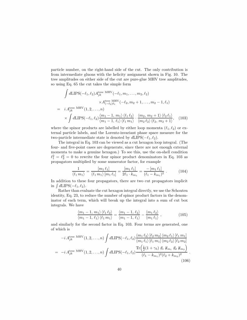
particle number, on the right-hand side of the cut. The only contribution isfrom intermediate gluons with the helicity assignment shown in Fig. 10. Thetree amplitudes on either side of the cut are pure-glue MHV tree amplitudes,so using Eq. 65 the cut takes the simple form

∫

dLIPS(−ℓ1, ℓ2)Atree MHVjk (−ℓ1, m1, . . . , m2, ℓ2)

×Atree MHV(−ℓ2)ℓ1

(−ℓ2, m2 + 1, . . . , m2 − 1, ℓ1)

= i Atree MHVjk (1, 2, . . . , n)

×∫

dLIPS(−ℓ1, ℓ2)〈m1 − 1, m1〉 〈ℓ1 ℓ2〉〈m1 − 1, ℓ1〉 〈ℓ1 m1〉

· 〈m2, m2 + 1〉 〈ℓ2 ℓ1〉〈m2 ℓ2〉 〈ℓ2, m2 + 1〉 , (103)

where the spinor products are labelled by either loop momenta (ℓ1, ℓ2) or ex-ternal particle labels, and the Lorentz-invariant phase space measure for thetwo-particle intermediate state is denoted by dLIPS(−ℓ1, ℓ2).

The integral in Eq. 103 can be viewed as a cut hexagon loop integral. (Thefour- and five-point cases are degenerate, since there are not enough externalmomenta to make a genuine hexagon.) To see this, use the on-shell conditionℓ21 = ℓ2

2 = 0 to rewrite the four spinor product denominators in Eq. 103 aspropagators multiplied by some numerator factor, for example

1

〈ℓ1 m1〉=

[m1 ℓ1]

〈ℓ1 m1〉 [m1 ℓ1]=

[m1 ℓ1]

2ℓ1 · km1

=− [m1 ℓ1]

(ℓ1 − km1)2

. (104)

In addition to these four propagators, there are two cut propagators implicitin

∫

dLIPS(−ℓ1, ℓ2).Rather than evaluate the cut hexagon integral directly, we use the Schouten

identity, Eq. 23, to reduce the number of spinor product factors in the denom-inator of each term, which will break up the integral into a sum of cut boxintegrals. We have

〈m1 − 1, m1〉 〈ℓ1 ℓ2〉〈m1 − 1, ℓ1〉 〈ℓ1 m1〉

=〈m1 − 1, ℓ2〉〈m1 − 1, ℓ1〉

− 〈m1 ℓ2〉〈m1 ℓ1〉

, (105)

and similarly for the second factor in Eq. 103. Four terms are generated, oneof which is

−i Atree MHVjk (1, 2, . . . , n)

∫

dLIPS(−ℓ1, ℓ2)〈m1 ℓ2〉 [ℓ2 m2] 〈m2 ℓ1〉 [ℓ1 m1]

〈m1 ℓ1〉 [ℓ1 m1] 〈m2 ℓ2〉 [ℓ2 m2]

= −i Atree MHVjk (1, 2, . . . , n)

∫

dLIPS(−ℓ1, ℓ2)Tr

(

12 (1 + γ5) 6ℓ1 6km1 6ℓ2 6km2

)

(ℓ1 − km1)2(ℓ2 + km2)

2.

(106)

40

This is the cut box integral Im1,m2

4 , where the set of momenta flowing out ofits four vertices is {km1 , Pm1+1,m2−1, km2 , Pm2+1,m1−1}. The other three terms

similarly give Im1−1,m2

4 , Im1,m2+14 and Im1−1,m2+1

4 , all with two loop momentainserted in the numerator.

The γ5-odd part of the trace in Eq. 106 does not contribute, because thebox does not have enough independent momenta to satisfy the Levi-Civitatensor. The γ5-even part can be reduced by standard Passarino-Veltman tech-niques39 to scalar box, triangle and bubble integrals. The coefficient of thescalar box integral Im1,m2

4 [1] is

− 12

(

P 2m1,m2−1P

2m1+1,m2

− P 2m1,m2

P 2m1+1,m2−1

)

. (107)

After summing over the four box integrals, the triangles and bubbles cancel out.(This could have been anticipated from the exercise in Section 4.1, showing thatAN=4 exhibits loop-momentum cancellations down to ℓm−4, plus the generalloop integral reduction procedures discussed in Section 4.2.) Therefore theN = 4 MHV amplitude which matches all the cuts is a sum of scalar boxintegrals, with coefficients given by Eq. 107, which evaluates explicitly (throughO(ǫ0)) to

AN=4n;1 (1+, . . . , j−, . . . , k−, . . . , n+) = (µ2)ǫ cΓ Atree MHV

jk (1, 2, . . . , n)Vn , (108)

where the universal, cyclically symmetric function Vn is given by

V2m+1 =

m−1∑

r=1

n∑

i=1

fi,r ,

V2m =

m−2∑

r=1

n∑

i=1

fi,r +

n/2∑

i=1

fi,m−1 , (109)

with

fi,r = − 1

ǫ2

[

(

−P 2i−1,i+r−1

)−ǫ+

(

−P 2i,i+r

)−ǫ −(

−P 2i,i+r−1

)−ǫ −(

−P 2i−1,i+r

)−ǫ]

+ Li2

(

1 −P 2

i,i+r−1

P 2i−1,i+r−1

)

+ Li2

(

1 −P 2

i,i+r−1

P 2i,i+r

)

+ Li2

(

1 −P 2

i−1,i+r

P 2i−1,i+r−1

)

+ Li2

(

1 −P 2

i−1,i+r

P 2i,i+r

)

−Li2

(

1 −P 2

i,i+r−1P2i−1,i+r

P 2i−1,i+r−1P

2i,i+r

)

+1

2ln2

(

P 2i−1,i+r−1

P 2i,i+r

)

. (110)

41

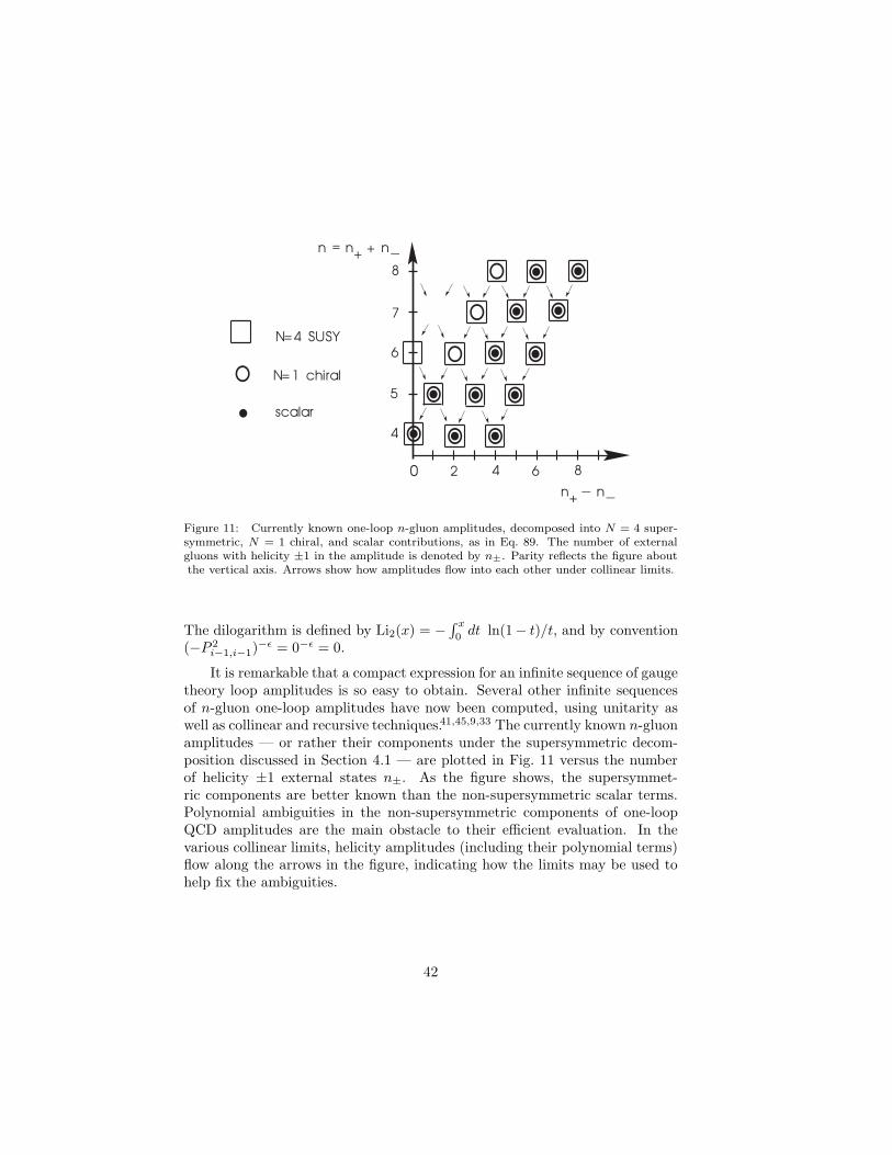
Figure 11: Currently known one-loop n-gluon amplitudes, decomposed into N = 4 super-symmetric, N = 1 chiral, and scalar contributions, as in Eq. 89. The number of externalgluons with helicity ±1 in the amplitude is denoted by n±. Parity reflects the figure aboutthe vertical axis. Arrows show how amplitudes flow into each other under collinear limits.

The dilogarithm is defined by Li2(x) = −∫ x

0 dt ln(1− t)/t, and by convention(−P 2

i−1,i−1)−ǫ = 0−ǫ = 0.

It is remarkable that a compact expression for an infinite sequence of gaugetheory loop amplitudes is so easy to obtain. Several other infinite sequencesof n-gluon one-loop amplitudes have now been computed, using unitarity aswell as collinear and recursive techniques.41,45,9,33 The currently known n-gluonamplitudes — or rather their components under the supersymmetric decom-position discussed in Section 4.1 — are plotted in Fig. 11 versus the numberof helicity ±1 external states n±. As the figure shows, the supersymmet-ric components are better known than the non-supersymmetric scalar terms.Polynomial ambiguities in the non-supersymmetric components of one-loopQCD amplitudes are the main obstacle to their efficient evaluation. In thevarious collinear limits, helicity amplitudes (including their polynomial terms)flow along the arrows in the figure, indicating how the limits may be used tohelp fix the ambiguities.

42

5 Conclusions

In these lectures we described techniques for efficient analytical calculation ofscattering amplitudes in gauge theories, particularly QCD. Tools such as he-licity and color decompositions, special gauges, unitarity, factorization limitsand supersymmetric rearrangements can lead to many simplifications. Some ofthese ideas can be motivated from string theory, but none requires its detailedknowledge. There is no one “magic bullet” but rather a combined arsenalof techniques that work well together. At the practical level, some of thesetools have been instrumental in calculating the one-loop five-parton ampli-tudes (ggggg, qqqqg and qqggg) which form the analytical bottleneck to NLOcross-sections for three-jet events at hadron colliders.28,46,10 They have alsobeen used to obtain infinite sequences of special one-loop helicity amplitudesin closed form.41,45,9,33 On the other hand, many processes of experimentalinterest remain uncalculated at NLO and at higher orders, so there is plentyof room for improvement in the field!

Acknowledgements

I would like to thank my collaborators, Zvi Bern, Dave Dunbar and DavidKosower, for contributing greatly to my understanding of the lecture topics;Zvi Bern, Michael Peskin and Wing Kai Wong for reading the manuscript; thestudents at TASI95 for very enjoyable discussions; and particularly DavisonSoper for organizing such a well-run school. This work was supported in partby a NATO Collaborative Research Grant CRG–921322.

References

1. CDF collaboration, Phys. Rev. Lett. 74:2626 (1995), Phys. Rev. D51:4623(1995); D0 collaboration, Phys. Rev. Lett. 74:2632 (1995).

2. Z. Kunszt, in these proceedings.3. M. Mangano and S. Parke, Phys. Rep. 200:301 (1991).4. Z. Bern and D.A. Kosower, Phys. Rev. Lett. 66:1669 (1991); Z. Bern

and D.A. Kosower, in Proceedings of the PASCOS-91 Symposium, eds.P. Nath and S. Reucroft (World Scientific, 1992); Z. Bern, Phys. Lett.296B:85 (1992).

5. Z. Bern and D.A. Kosower, Nucl. Phys. B379:451 (1992).6. F.A. Berends and W.T. Giele, Nucl. Phys. B294:700 (1987); M. Mangano,

S. Parke and Z. Xu, Nucl. Phys. B298:653 (1988); M. Mangano, Nucl.Phys. B309:461 (1988).

43

7. Z. Bern and D.A. Kosower, Nucl. Phys. B362:389 (1991).8. G. ’t Hooft, Nucl. Phys. B72:461 (1974); Nucl. Phys. B75:461 (1974);

P. Cvitanovic, Group Theory (Nordita, 1984).9. Z. Bern, L. Dixon, D.C. Dunbar and D.A. Kosower, Nucl. Phys. B425:217

(1994).10. Z. Bern, L. Dixon and D.A. Kosower, Nucl. Phys. B437:259 (1995).11. F.A. Berends, R. Kleiss, P. De Causmaecker, R. Gastmans and T.T.

Wu, Phys. Lett. B103:124 (1981); P. De Causmaeker, R. Gastmans,W. Troost and T.T. Wu, Nucl. Phys. B206:53 (1982); R. Kleiss andW.J. Stirling, Nucl. Phys. B262:235 (1985); R. Gastmans and T.T. Wu,The Ubiquitous Photon: Helicity Method for QED and QCD (ClarendonPress, 1990).

12. Z. Xu, D.-H. Zhang and L. Chang, Nucl. Phys. B291:392 (1987).13. J.F. Gunion and Z. Kunszt, Phys. Lett. 161B:333 (1985).14. S.J. Parke and T. Taylor, Phys. Lett. 157B:81 (1985); Z. Kunszt, Nucl.

Phys. B271:333 (1986).15. F.A. Berends and W.T. Giele, Nucl. Phys. B306:759 (1988).16. D.A. Kosower, Nucl. Phys. B335:23 (1990).17. S.J. Parke and T.R. Taylor, Phys. Rev. Lett. 56:2459 (1986).18. Z. Kunszt and W.J. Stirling, Phys. Rev. D37:2439 (1988); C.J. Maxwell,

Phys. Lett. B192:190 (1987).19. M.T. Grisaru, H.N. Pendleton and P. van Nieuwenhuizen, Phys. Rev.

D15:996 (1977); M.T. Grisaru and H.N. Pendleton, Nucl. Phys. B124:81(1977).

20. F.A. Berends and W.T. Giele, Nucl. Phys. B313:595 (1989).21. M. Mangano and S. J. Parke, Nucl. Phys. B299:673 (1988).22. G. Altarelli and G. Parisi, Nucl. Phys. B126:298 (1977).23. G. Sterman, in these proceedings.24. A. Signer, Phys. Lett. B357:204 (1995).25. A. Signer, Ph.D. Thesis, ETH-Zurich (1995).26. R. Kleiss and W.J. Stirling, Nucl. Phys. B262:235 (1985); A. Ballestrero

and E. Maina, Phys. Lett. B350:225 (1995); S. Dittmaier, Wurzburgpreprint 93-0023.

27. R. Vega and J. Wudka, preprint hep-ph/9511310.28. Z. Bern, L. Dixon and D.A. Kosower, Phys. Rev. Lett. 70:2677 (1993).29. G. ’t Hooft, in Acta Universitatis Wratislavensis no. 38, 12th Winter

School of Theoretical Physics in Karpacz, Functional and ProbabilisticMethods in Quantum Field Theory, Vol. 1 (1975) ; B.S. DeWitt, inQuantum gravity II, eds. C. Isham, R. Penrose and D. Sciama (Oxford,1981); L.F. Abbott, Nucl. Phys. B185:189 (1981); L.F. Abbott, M.T.

44

Grisaru and R.K. Schaefer, Nucl. Phys. B229:372 (1983).30. W. Siegel, Phys. Lett. 84B:193 (1979); D.M. Capper, D.R.T. Jones and

P. van Nieuwenhuizen, Nucl. Phys. B167:479 (1980); L.V. Avdeev andA.A. Vladimirov, Nucl. Phys. B219:262 (1983).

31. Z. Bern and D.C. Dunbar, Nucl. Phys. B379:562 (1992).32. A.G. Morgan, Phys. Lett. B351:249 (1995).33. Z. Bern, L. Dixon, D.C. Dunbar and D.A. Kosower, Nucl. Phys. B435:59

(1995).34. J.L. Gervais and A. Neveu, Nucl. Phys. B46:381 (1972).35. W. van Neerven and J. Vermaseren, Phys. Lett. 137B:241 (1984).36. D.B. Melrose, Il Nuovo Cimento 40A:181 (1965).37. Z. Bern, L. Dixon and D.A. Kosower, Phys. Lett. 302B:299 (1993);

erratum ibid. 318:649 (1993).38. Z. Bern, L. Dixon and D.A. Kosower, Nucl. Phys. B412:751 (1994).39. L.M. Brown and R.P. Feynman, Phys. Rev. 85:231 (1952) ; G. Pas-

sarino and M. Veltman, Nucl. Phys. B160:151 (1979); G. ’t Hooft andM. Veltman, Nucl. Phys. B153:365 (1979).

40. G.J. van Oldenborgh and J.A.M. Vermaseren, Z. Phys. C46:425 (1990);G.J. van Oldenborgh, Ph.D. thesis, University of Amsterdam (1990).

41. Z. Bern, G. Chalmers, L. Dixon and D.A. Kosower, Phys. Rev. Lett.72:2134 (1994).

42. Z. Bern and G. Chalmers, Nucl. Phys. B447:465 (1995).43. L.D. Landau, Nucl. Phys. 13:181 (1959); S. Mandelstam, Phys. Rev.

112:1344 (1958), 115:1741 (1959); R.E. Cutkosky, J. Math. Phys. 1:429(1960).

44. W.L. van Neerven, Nucl. Phys. B268:453 (1986); Z. Bern and A. Mor-gan, preprint hep-ph/11336; Z. Bern, L. Dixon and D.A. Kosower, toappear in Ann. Rev. Nucl. Part. Sci.

45. G.D. Mahlon, Phys. Rev. D49:2197 (1994); Phys. Rev. D49:4438 (1994).46. Z. Kunszt, A. Signer and Z. Trocsanyi, Phys. Lett. B336:529 (1994).

45