arX

iv:q

uant

-ph/

0209

120v

2 2

4 Se

p 20

02

A geometric theory of non-local two-qubit operations

Jun Zhang1, Jiri Vala2, K. Birgitta Whaley2 and Shankar Sastry11Department of Electrical Engineering and Computer Sciences

2 Department of Chemistry and Pitzer Center for Theoretical ChemistryUniversity of California, Berkeley, CA 94720

(Dated: October 31, 2018)

We study non-local two-qubit operations from a geometric perspective. By applying a Cartandecomposition to su(4), we find that the geometric structure of non-local gates is a 3-Torus. Wederive the invariants for local transformations, and connect these local invariants to the coordinatesof the 3-Torus. Since different points on the 3-Torus may correspond to the same local equivalenceclass, we use the Weyl group theory to reduce the symmetry. We show that the local equivalenceclasses of two-qubit gates are in one-to-one correspondence with the points in a tetrahedron excepton the base. We then study the properties of perfect entanglers, that is, the two-qubit operationsthat can generate maximally entangled states from some initially separable states. We providecriteria to determine whether a given two-qubit gate is a perfect entangler and establish a geometricdescription of perfect entanglers by making use of the tetrahedral representation of non-local gates.We find that exactly half the non-local gates are perfect entanglers. We also investigate the non-local operations generated by a given Hamiltonian. We first study the gates that can be directlygenerated by a Hamiltonian. Then we explicitly construct a quantum circuit that contains at mostthree non-local gates generated by a two-body interaction Hamiltonian, together with at most fourlocal gates generated by single qubit terms. We prove that such a quantum circuit can simulateany arbitrary two-qubit gate exactly, and hence it provides an efficient implementation of universalquantum computation and simulation.

I. INTRODUCTION

Considerable effort has been made on the characterization of non-local properties of quantum states and operations.Grassl et al. [1] have computed locally invariant polynomial functions of density matrix elements. Makhlin [2] hasrecently analyzed non-local properties of two-qubit gates and presented local invariants for an operation M ∈ U(4).Makhlin also studied some basic properties of perfect entanglers, which are defined as the unitary operations thatcan generate maximal entangled states from some initially separable states. Also shown were entangling properties ofgates generated by several different Hamiltonian operators. All these results are crucial for physical implementationsof quantum computation schemes.Determining the entangling capabilities of operations generated by a given physical system is another intriguing and

complementary issue. Zanardi [3, 4] has explored the entangling power of quantum evolutions. The most extensiverecent effort to characterize entangling operations is due to Cirac and coworkers [5, 6, 7, 8, 9, 10, 11, 12]. Kraus andCirac [8] focused on finding the best separable two-qubit input states such that some given unitary transformationcan create maximal entanglement. Vidal et al. [9] developed the interaction cost for a non-local operation as theoptimal time to generate it from a given Hamiltonian. The same group, Hammerer et al. [12] then extended theseconsiderations to characterize non-local gates. These works are closely related to time optimal control as addressedrecently by Khaneja et al. [13], who studied systems described by a Hamiltonian that contains both a non-local internalor drift term, and a local control term. All these studies assume that any single qubit operation can be achievedalmost instantaneously. This is a good approximation for the situation when the control terms in the Hamiltoniancan be made large compared to the internal couplings.Universality and controllability are issues of crucial importance in physical implementations of quantum information

processing [14, 15]. A series of important results have been obtained since questions of universality were first addressedby Deutsch in his seminal papers on quantum computing [16, 17]. Deutsch [17] proved that any unitary operationcan be constructed from generalized Toffoli gate operating on three qubits. DiVincenzo [18] proved universality fortwo-qubit gates by reconstructing three-qubit operations using these gates and a local NOT gate. Similarly, Barenco[19, 20] and Sleator and Weinfurter [21] identified the controlled unitary operation as a universal two-qubit gate.Barenco [22] showed the universality of the CNOT gate supplemented with any single qubit unitaries, and pointedout advantages of CNOT in the context of quantum information processing. Lloyd [23] showed that almost anyquantum gate for two or more qubits is universal. Deutsch et al. [24] proved that almost any two-qubit gate isuniversal by showing that the set of non-universal operations in U(4) is of lower dimension than the U(4) group.Universal properties of quantum gates acting on an n ≥ 2 dimensional Hilbert space have been studied by Brylinski[25]. Dodd et al. [26] have pointed out that universal quantum computation can be achieved by any entanglinggate supplemented with local operations. Bremner et al. [27] recently demonstrated this by extending the results

2

of Brylinski, giving a constructive proof that any two-qubit entangling gate can generate CNOT if arbitrary singlequbit operations are also available. Universal sets of quantum gates for n-qubit systems have been explored by Vlasov[28, 29] in connection with Clifford algebras.General results on efficient simulation of any unitary operation in SU(2n) by a discrete set of gates are embodied

in the Solovay-Kitaev theorem [15, 30] and in recent work due to Harrow et al. [31]. The Solovay-Kitaev theoremimplies the equivalence of different designs of universal quantum computers based on suitable discrete sets of single-qubit and two-qubit operations in a quantum circuit. An example is the standard universal set of gates includingcontrolled-NOT and three discrete single-qubit gates, namely Hadamard, Phase and π/2 gates [15]. Other universalsets have also been proposed. According to the Solovay-Kitaev theorem, every such design can represent a circuitthat is formulated using the standard set of gates. Consequently, all quantum computation constructions—includingalgorithms, error-correction, and fault-tolerance—can be efficiently simulated by physical systems that can provide asuitable set of operations, and do not necessarily need to be implemented by the standard gates. This moves the focusfrom study of gates to study of the Hamiltonians whose time evolution gives rise to the gates. In this context, Burkardet al. [32] studied the quantum computation potential of the isotropic exchange Hamiltonian. This interaction can

generate√SWAP gate directly. However, CNOT cannot be obtained directly from the exchange interaction. Burkard

et al. showed that it can be generated via a circuit of two√SWAP gates and a single-qubit phase rotation. More

recently, Whaley and co-workers have shown that the two-particle exchange interaction is universal when physicalqubits are encoded into logical qubits, allowing a universal gate set to be constructed from this interaction alone[33, 34, 35, 36, 37, 38]. This has given rise to the notion of “encoded universality”, in which a convenient physicalinteraction is made universal by encoding into a subspace [35, 36]. Isotropic, anisotropic, and generalized forms of theexchange interaction have recently been shown to possess considerable power for efficient construction of universalgate sets, allowing explicit universal gate constructions that require only a small number of physical operations[34, 37, 38, 39].In this paper, we analyze non-local two-qubit operations from a geometric perspective and show that considerable

insight can be achieved with this approach. We are concerned with three main questions here. First, achieving ageometric representation of two-qubit gates. Second, characterizing or quantifying all operations that can generatemaximal entanglement. Third, exact simulation of any arbitrary two-qubit gates from a given two-body physicalinteraction together with single qubit gates. The fundamental mathematical techniques we employ are Cartan decom-position and Weyl group in the Lie group representation theory. The application of these theories to the Lie algebrasu(4) provides us with a natural and intuitive geometric approach to investigate the properties of non-local two-qubitoperations. This geometric approach reveals the nature of the problems intrinsically and allows a general formulationof solutions to the three issues of interest here.Because it is the non-local properties that generate entanglement in quantum systems, we first study the invariants

and geometric representation of non-local two-qubit operations. A pair of two-qubit operations are called locallyequivalent if they differ only by local operations. We apply the Cartan decomposition theorem to su(4), the Liealgebra of the special unitary group SU(4). We find that the geometric structure of non-local gates is a 3-Torus.On the other hand, the Cartan decomposition of su(4) derived from the complexification of sl(4) yields an easy wayto derive the invariants for local transformations. These invariants can be used to determine whether two gates arelocally equivalent. Moreover, we establish the relation of these local invariants to the coordinates of the 3-Torus.This provides with a way to compute the corresponding points on the 3-Torus for a given gate. It turns out that asingle non-local gate may correspond to finitely many different points on the 3-Torus. If we represent these pointsin a cube with side length π, there is obvious symmetry between these points. We then use the Weyl group theoryto reduce this symmetry. We know that in this case the Weyl group is generated by a set of reflections in R3. It isthese reflections that create the kaleidoscopic symmetry of points that correspond to the same non-local gate in thecube. We can explicitly compute these reflections, and thereby show that the local equivalence classes of two-qubitgates are in one-to-one correspondence with the points in a tetrahedron except on the base. This provides a completegeometric representation of non-local two-qubit operations.The second objective of this paper is to explore the properties of perfect entanglers, that is, the quantum gates that

can generate maximally entangled states from some initially separable states. We start with criteria to determinewhether a given two-qubit gate is a perfect entangler. A condition for such a gate has been stated in [2]. Weprovide here a proof of this condition and show that the condition can be employed within our geometric analysis todetermine which fraction of all non-local two-qubit gates are perfect entanglers. We show that the entangling propertyof a quantum gate is only determined by its geometric representation on the 3-Torus. Using the result that every pointon the tetrahedron corresponds to a local equivalence class, we then show that the set of all perfect entanglers is apolyhedron with seven faces and possessing a volume equal to exactly half that of the tetrahedron. This implies thatamongst all the non-local two-qubit operations, exactly half of them are capable of generating maximal entanglement.Finally, we explore universality and controllability aspects of non-local properties of given physical interactions

and the potential of such specified Hamiltonians to generate perfect entanglers. Our motivation is related to that of

3

PSfrag replacements

Local Gates

Non-Perfect Entanglers

Perfect Entanglers

CNOT

Non-local Gates

SU(4)\SU(2) ⊗ SU(2)

SU(2)⊗ SU(2)

SWAP

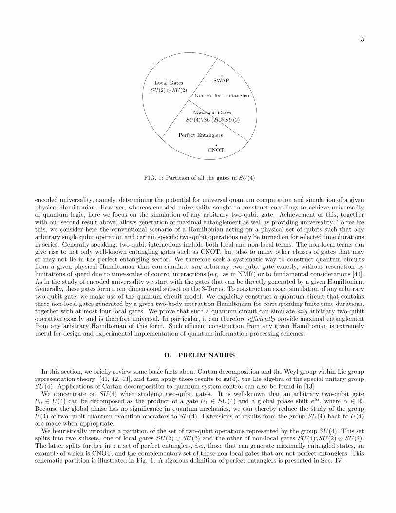
FIG. 1: Partition of all the gates in SU(4)

encoded universality, namely, determining the potential for universal quantum computation and simulation of a givenphysical Hamiltonian. However, whereas encoded universality sought to construct encodings to achieve universalityof quantum logic, here we focus on the simulation of any arbitrary two-qubit gate. Achievement of this, togetherwith our second result above, allows generation of maximal entanglement as well as providing universality. To realizethis, we consider here the conventional scenario of a Hamiltonian acting on a physical set of qubits such that anyarbitrary single qubit operation and certain specific two-qubit operations may be turned on for selected time durationsin series. Generally speaking, two-qubit interactions include both local and non-local terms. The non-local terms cangive rise to not only well-known entangling gates such as CNOT, but also to many other classes of gates that mayor may not lie in the perfect entangling sector. We therefore seek a systematic way to construct quantum circuitsfrom a given physical Hamiltonian that can simulate any arbitrary two-qubit gate exactly, without restriction bylimitations of speed due to time-scales of control interactions (e.g. as in NMR) or to fundamental considerations [40].As in the study of encoded universality we start with the gates that can be directly generated by a given Hamiltonian.Generally, these gates form a one dimensional subset on the 3-Torus. To construct an exact simulation of any arbitrarytwo-qubit gate, we make use of the quantum circuit model. We explicitly construct a quantum circuit that containsthree non-local gates generated by a given two-body interaction Hamiltonian for corresponding finite time durations,together with at most four local gates. We prove that such a quantum circuit can simulate any arbitrary two-qubitoperation exactly and is therefore universal. In particular, it can therefore efficiently provide maximal entanglementfrom any arbitrary Hamiltonian of this form. Such efficient construction from any given Hamiltonian is extremelyuseful for design and experimental implementation of quantum information processing schemes.

II. PRELIMINARIES

In this section, we briefly review some basic facts about Cartan decomposition and the Weyl group within Lie grouprepresentation theory [41, 42, 43], and then apply these results to su(4), the Lie algebra of the special unitary groupSU(4). Applications of Cartan decomposition to quantum system control can also be found in [13].We concentrate on SU(4) when studying two-qubit gates. It is well-known that an arbitrary two-qubit gate

U0 ∈ U(4) can be decomposed as the product of a gate U1 ∈ SU(4) and a global phase shift eiα, where α ∈ R.Because the global phase has no significance in quantum mechanics, we can thereby reduce the study of the groupU(4) of two-qubit quantum evolution operators to SU(4). Extensions of results from the group SU(4) back to U(4)are made when appropriate.We heuristically introduce a partition of the set of two-qubit operations represented by the group SU(4). This set

splits into two subsets, one of local gates SU(2) ⊗ SU(2) and the other of non-local gates SU(4)\SU(2) ⊗ SU(2).The latter splits further into a set of perfect entanglers, i.e., those that can generate maximally entangled states, anexample of which is CNOT, and the complementary set of those non-local gates that are not perfect entanglers. Thisschematic partition is illustrated in Fig. 1. A rigorous definition of perfect entanglers is presented in Sec. IV.

4

A. Cartan decomposition and Weyl group

Our first goal is to establish fundamentals for a geometric picture of non-local unitary operations with emphasison their generators, which are represented by Hamiltonian operators in physical context. We start with a summaryof some basic definitions [41, 42, 43]. Consider a Lie group G and its corresponding Lie algebra g. The adjointrepresentation Adg is a map from the Lie algebra g to g which is the differential of the conjugation map ag fromthe Lie group G to G given by ag(h) = ghg−1. For matrix Lie algebras, Adg(Y ) = gY g−1, where g, Y are bothrepresented as matrices of compatible dimensions. The differential of the adjoint representation is denoted by ad, andadX is a map from the Lie algebra g to g given by the Lie bracket with X , that is, adX(Y ) = [X,Y ].We now define an inner product on g by the Killing form B(X,Y ) = tr(adX adY ). Let {X1, . . . , Xn} be a basis for

g. The numbers Cijk ∈ C such that

[Xj , Xk] =

n∑

i=1

CijkXi (1)

are the structure constants of the Lie algebra g with respect to the basis, where j, k run from 1 to n. Since

adXj[X1, . . . , Xn] = [

n∑

i=1

Cij1Xi, . . . ,

n∑

i=1

CijnXi]

= [X1, . . . , Xn]

C1j1 · · · C1

jn

......

Cnj1 · · · Cnjn

,

(2)

the matrix representation of adXjwith respect to the basis is

C1j1 · · · C1

jn

......

Cnj1 · · · Cnjn

. (3)

Thus, the trace of adXjadXk

, which is B(Xj , Xk), is∑n

a,b=1 CajbCbka, which is also the jk-th entry of the matrix of

the quadratic form B( , ). The Lie algebra g is semisimple if and only if the Killing form is nondegenerate, i.e., thedeterminant of its matrix is nonzero.Let K be a compact subgroup of G, and k the Lie algebra of K. Assume that g admits a direct sum decomposition

g = p⊕ k, such that p = k⊥ with respect to the metric induced by the inner product.

Definition 1 (Cartan decomposition of the Lie algebra g) Let g be a semisimple Lie algebra and let the de-composition g = p⊕ k, p = k⊥ satisfy the commutation relations

[k, k] ⊂ k, [p, k] ⊂ p, [p, p] ⊂ k. (4)

This decomposition is called a Cartan decomposition of g, and the pair (g, k) is called an orthogonal symmetric Lie

algebra pair.

A maximal Abelian subalgebra a contained in p is called a Cartan subalgebra of the pair (g, k). If a′ is another Cartansubalgebra of (g, k), then there exists an element k ∈ K such that Adk(a) = a′. Moreover, we have p = ∪k∈K Adk(a).

Proposition 1 (Decomposition of the Lie group G) Given a semisimple Lie algebra g and its Cartan decompo-

sition g = p⊕ k, let a be a Cartan subalgebra of the pair (g, k), then G = K exp(a)K.

For X ∈ a, let W ∈ g be an eigenvector of adX and α(X) the corresponding eigenvalue, i.e.,

[X,W ] = α(X)W. (5)

The linear function α is called a root of g with respect to a. Let ∆ denote the set of nonzero roots, and ∆p denotethe set of roots in ∆ which do not vanish identically on a. Note that if α ∈ ∆, it is also true that −α ∈ ∆.Let M and M ′ denote the centralizer and normalizer of a in K, respectively. In other words,

M = {k ∈ K|Adk(X) = X for each X ∈ a},M ′ = {k ∈ K|Adk(a) ⊂ a}. (6)

5

Definition 2 (Weyl group) The quotient group M ′/M is called the Weyl group of the pair (G,K). It is denoted

by W (G,K).

One can prove that W (G,K) is a finite group. Each α ∈ ∆p defines a hyperplane α(X) = 0 in the vector space a.These hyperplanes divide the space a into finitely many connected components, called the Weyl chambers. For eachα ∈ ∆p, let sα denote the reflection with respect to the hyperplane α(X) = 0 in a.

Proposition 2 (Generation of the Weyl group) The Weyl group is generated by the reflections sα, α ∈ ∆p.

This proposition is proved in Corollary 2.13, Ch. VII in [41].

B. Application to su(4)

Now we apply the above results to su(4), the Lie algebra of the special unitary group SU(4). The Lie algebrag = su(4) has a direct sum decomposition g = p⊕ k, where

k = spani

2{σ1

x, σ1y, σ

1z , σ

2x, σ

2y , σ

2z},

p = spani

2{σ1

xσ2x, σ

1xσ

2y, σ

1xσ

2z , σ

1yσ

2x, σ

1yσ

2y, σ

1yσ

2z , σ

1zσ

2x, σ

1zσ

2y, σ

1zσ

2z}.

(7)

Here σx, σy, and σz are the Pauli matrices, and σ1ασ

2β = σ1

α ⊗ σ2β . If we use Xj to denote the matrices in Eq. (7),

where j runs from left to right in Eq. (7), we can derive the Lie brackets of Xj and Xk. These are summarized inthe following table:

[Xj , Xk] X1 X2 X3 X4 X5 X6 X7 X8 X9 X10 X11 X12 X13 X14 X15

X1 0 −X3 X2 0 0 0 0 0 0 −X13 −X14 −X15 X10 X11 X12

X2 X3 0 −X1 0 0 0 X13 X14 X15 0 0 0 −X7 −X8 −X9

X3 −X2 X1 0 0 0 0 −X10 −X11 −X12 X7 X8 X9 0 0 0

X4 0 0 0 0 −X6 X5 0 −X9 X8 0 −X12 X11 0 −X15 X14

X5 0 0 0 X6 0 −X4 X9 0 −X7 X12 0 −X10 X15 0 −X13

X6 0 0 0 −X5 X4 0 −X8 X7 0 −X11 X10 0 −X14 X13 0

X7 0 −X13 X10 0 −X9 X8 0 −X6 X5 −X3 0 0 X2 0 0

X8 0 −X14 X11 X9 0 −X7 X6 0 −X4 0 −X3 0 0 X2 0

X9 0 −X15 X12 −X8 X7 0 −X5 X4 0 0 0 −X3 0 0 X2

X10 X13 0 −X7 0 −X12 X11 X3 0 0 0 −X6 X5 −X1 0 0

X11 X14 0 −X8 X12 0 −X10 0 X3 0 X6 0 −X4 0 −X1 0

X12 X15 0 −X9 −X11 X10 0 0 0 X3 −X5 X4 0 0 0 −X1

X13 −X10 X7 0 0 −X15 X14 −X2 0 0 X1 0 0 0 −X6 X5

X14 −X11 X8 0 X15 0 −X13 0 −X2 0 0 X1 0 X6 0 −X4

X15 −X12 X9 0 −X14 X13 0 0 0 −X2 0 0 X1 −X5 X4 0

Now the structure constants Cijk can be found from the above table (see Eq. (1)) so that we can evaluate

B(Xj , Xk) =

15∑

a=1

15∑

b=1

CajbCbka = −8δjk. (8)

It is easy to verify that tr(XjXk) = −δjk, and thus the Killing form of su(4) is B(X,Y ) = 8 tr(XY ). Since k =span {X1, . . . , X6} and p = span {X7, . . . , X15}, from the Lie bracket computation table above, it is clear that

[k, k] ⊂ k, [p, k] ⊂ p, [p, p] ⊂ k. (9)

Therefore the decomposition g = k⊕ p is a Cartan decomposition of su(4). Note that the Abelian subalgebra

a = spani

2{σ1

xσ2x, σ

1yσ

2y , σ

1zσ

2z} (10)

6

is contained in p and is a maximal Abelian subalgebra, i.e., we cannot find any other Abelian subalgebra of p thatcontains a. Hence it is a Cartan subalgebra of the pair (g, k). Further, since the set of all the local gates K is aconnected Lie subgroup SU(2) ⊗ SU(2) of SU(4), and there is one-to-one correspondence between connected Liesubgroups of a Lie group and subalgebras of its Lie algebra [44], it is clear that k in Eq. (7) is just the Lie subalgebracorresponding to K. From Proposition 1, any U ∈ SU(4) can be decomposed as

U = k1Ak2 = k1 exp{i

2(c1σ

1xσ

2x + c2σ

1yσ

2y + c3σ

1zσ

2z)}k2, (11)

where k1, k2 ∈ SU(2)⊗ SU(2), and c1, c2, c3 ∈ R.Another more intuitive Cartan decomposition of su(4) can be obtained via the complexification of sl(4). Consider

G = SL(4), the real special linear group, and K = SO(4), the special orthogonal group. The Lie algebra sl(4) isthe set of 4 × 4 real matrices of trace zero, and so(4) the set of 4 × 4 real skew symmetric matrices. Then sl(4) canbe decomposed as sl(4) = so(4) ⊕ p, where p is the set of 4 × 4 real symmetric matrices. This is nothing but thedecomposition of a matrix into symmetric and skew symmetric parts, and it is indeed a Cartan decomposition ofsl(4). Consider the following subset of the complexification of sl(4):

gµ = so(4) + ip. (12)

It can be verified that gµ is exactly su(4), and thus (gµ, so(4)) is an orthogonal symmetric Lie algebra pair. Theisomorphism carrying k in Eq. (7) into so(4) is just the transformation from the standard computational basis ofstates to the Bell basis in [2, 12]. This procedure is of crucial importance in computing the invariants for two-qubitgates under local transformations. See Section III for more details.Now let us compute the Weyl groupW (G,K). Let X = i

2 (c1σ1xσ

2x+ c2σ

1yσ

2y+ c3σ

1zσ

2z) ∈ a. Identify a with R3, then

X = [c1, c2, c3]. The roots of g with respect to a are eigenvalues of the matrix of adX :

∆p = i{c1 − c2,−c1 − c2,−c1 − c3, c1 − c3, c2 − c3, c2 + c3,

− c1 + c2, c1 + c2, c1 + c3,−c1 + c3,−c2 + c3,−c2 − c3}.(13)

For α = i(c1 − c3) ∈ ∆p, the plane α(X) = 0 in a is the set {X ∈ R3|uTX = 0}, where u = [1, 0,−1]T . The reflectionof X = [c1, c2, c3] with respect to the plane α(X) = 0 is

sα(X) = X − 2uuT

‖u‖2 X = [c3, c2, c1]. (14)

Similarly, we can compute all the reflections sα as follows:

si(c3−c2)(X) = [c1, c3, c2], si(c2+c3)(X) = [c1,−c3,−c2],si(c2−c1)(X) = [c2, c1, c3], si(c1+c2)(X) = [−c2,−c1, c3],si(c1−c3)(X) = [c3, c2, c1], si(c1+c3)(X) = [−c3, c2,−c1].

(15)

From Proposition 2, the Weyl group W (G,K) is generated by sα given in Eq. (15). Therefore, the reflections sα areequivalent to either permutations of the elements of [c1, c2, c3], or permutations with sign flips of two elements.

III. NON-LOCAL OPERATIONS

We now study non-local two-qubit operations within the group theoretical framework of the previous section. TheCartan decomposition of su(4) provides us with a good starting point to explore the invariants under local gateoperations. It also reveals that the geometric structure of the local equivalence classes is none other than a 3-Torus.Every point on this 3-Torus corresponds to a local equivalence class of two-qubit gates. Different points may alsocorrespond to the same equivalence class. To reduce this symmetry, we apply the Weyl group theory. We show thatthe local equivalence classes of two-qubit gates are in one-to-one correspondence with the points in a tetrahedron,except on the base where there are two equivalent areas. This tetrahedral representation of non-local operations playsa central role in our subsequent discussion of perfect entanglers and the design of universal quantum circuits.

A. Local invariants and local equivalence classes

Two unitary transformations U , U1 ∈ SU(4) are called locally equivalent if they differ only by local operations:U = k1U1k2, where k1, k2 ∈ SU(2) ⊗ SU(2) are local gates. This clearly defines an equivalence relation on the Lie

7

group SU(4). We denote the equivalence class of a unitary transformation U as [U ]. From the Cartan decompositionof su(4) in Section II B, any two-qubit gate U ∈ SU(4) can be written in the following form

U = k1Ak2 = k1 exp{i

2(c1σ

1xσ

2x + c2σ

1yσ

2y + c3σ

1zσ

2z)}k2, (16)

where k1, k2 ∈ SU(2)⊗ SU(2). Because the two-qubit gate U is periodic in ck and the minimum positive period isπ, the geometric structure of [c1, c2, c3] is a 3-Torus, T 3 = S1 × S1 × S1.In [2], local invariants were given for two-qubit gates. Here we will connect these invariants of Makhlin to the

coordinates [c1, c2, c3] on the 3-Torus. We first consider the case of the two-qubit gates in SU(4), and then extendthe results to the general case of U(4).

1. SU(4) Operations

Consider the transformation from the standard basis of states |00〉, |01〉, |10〉, |11〉 to the Bell basis |Φ+〉 =1√2(|00〉+ |11〉), |Φ−〉 = i√

2(|01〉+ |10〉), |Ψ+〉 = 1√

2(|01〉 − |10〉), |Ψ−〉 = i√

2(|00〉 − |11〉). In this basis, the two-qubit

gate U in Eq. (16) can be written as

UB = Q†UQ = Q†k1Ak2Q, (17)

where

Q =1√2

1 0 0 i

0 i 1 0

0 i −1 0

1 0 0 −i

. (18)

Recalling that i2{σ1

x, σ1y, σ

1z , σ

2x, σ

2y, σ

2z} is a basis for k, it is not hard to verify that i

2Q†{σ1

x, σ1y, σ

1z , σ

2x, σ

2y, σ

2z}Q forms

a basis for so(4), the Lie algebra of the special orthogonal group SO(4). Hence UB can be written as

UB = O1Q†AQO2, (19)

where

O1 = Q†k1Q ∈ SO(4),

O2 = Q†k2Q ∈ SO(4).(20)

Eq. (19) can also be obtained from the Cartan decomposition of su(4) derived from the complexification of sl(4), asdiscussed in Section II B. An Abelian subalgebra a is generated by i

2{σ1xσ

2x, σ

1yσ

2y, σ

1zσ

2z}, and the transformation to

the Bell basis takes these operators to i2{σ1

z ,−σ2z , σ

1zσ

2z}. Therefore, we have UB = O1FO2, where

F = Q†AQ

= exp{ i2(c1σ

1z − c2σ

2z + c3σ

1zσ

2z)}

= diag{eic1−c2+c3

2 , eic1+c2−c3

2 , e−ic1+c2+c3

2 , ei−c1+c2+c3

2 }.

(21)

Let

m = UTBUB = OT2 F2O2, (22)

where O2 is defined by Eq. (20). The complete set of local invariants of a two-qubit gate U ∈ SU(4) is given by thespectrum of the matrix m [2], and hence by the eigenvalues of F 2:

{ ei(c1−c2+c3), ei(c1+c2−c3), e−i(c1+c2+c3), ei(−c1+c2+c3)}. (23)

Since m is unitary and detm = 1, the characteristic polynomial of m is then

|sI −m| = s4 − tr(m) s3 +1

2

(

tr2(m)− tr(m2))

s2 − tr(m) s+ 1. (24)

Therefore the spectrum of m is completely determined by only the two quantities tr(m) and tr2(m)− tr (m2). For atwo-qubit gate U given in Eq. (16), its local invariants can be derived from Eq. (23) as:

tr (m) = 4 cos c1 cos c2 cos c3 + 4i sin c1 sin c2 sin c3,

tr2 (m)− tr (m2) = 16 cos2 c1 cos2 c2 cos

2 c3 − 16 sin2 c1 sin2 c2 sin

2 c3 − 4 cos 2c1 cos 2c2 cos 2c3.(25)

8

2. Generalization to U(4)

Now let us consider the local invariants for the general case of U(4) [2]. An arbitrary two-qubit gate U ∈ U(4) canbe decomposed as the product of a gate U1 ∈ SU(4) and a global phase shift eiα, where detU = ei4α. It follows thatm(U1) = e−i2αm(U), where

m(U) = (Q†UQ)TQ†UQ, (26)

and

tr(

m(U1))

= e−i2α tr(

m(U))

,

tr2(

m(U1))

− tr(

m2(U1))

= e−i4α(

tr2(m(U))− tr(m2(U)))

.(27)

It is clear that the global phase factor just rotates the eigenvalues of m(U) along the unit circle in the complexplane, while keeping their relative phase invariant. Therefore, it does not affect the entangling properties and we canconsequently divide by det(U). The local invariants of a two-qubit gate U are thus given by

G1 =tr2

(

m(U))

16 detU,

G2 =tr2

(

m(U))

− tr(

m2(U))

4 detU,

(28)

where the numerical factors are incorporated into the denominators to provide convenient normalization. If U is nowwritten in the following form:

U = eiαk1Ak2 = eiαk1 exp{i

2(c1σ

1xσ

2x + c2σ

1yσ

2y + c3σ

1zσ

2z)}k2, (29)

we can compute its local invariants as:

G1 = cos2 c1 cos2 c2 cos

2 c3 − sin2 c1 sin2 c2 sin

2 c3 +i

4sin 2c1 sin 2c2 sin 2c3

G2 = 4 cos2 c1 cos2 c2 cos

2 c3 − 4 sin2 c1 sin2 c2 sin

2 c3 − cos 2c1 cos 2c2 cos 2c3.(30)

Because the local invariants G1 and G2 characterize the non-local properties of unitary operations, we can usethese two invariants to check whether a pair of two-qubit gates are locally equivalent. The invariants G1 and G2

are evaluated by taking the matrix representation of a gate in the Bell basis and then using Eqs. (26) and (28). Forexample, CNOT and Controlled-Z (referred as C(Z)) possess identical values of the local invariants, given by G1 = 0and G2 = 1. Therefore, they belong to the same local equivalence class. We refer to this class as [CNOT]. On the

other hand, the local invariants for√SWAP are G1 = i/4 and G2 = 0. Hence this gate belongs to a different local

equivalence class that we refer to as [√SWAP]. Note that from Eq. (28), since the local invariants are functions of

eigenvalues of the matrix m, the local equivalence class can alternatively be defined simply via the set of eigenvaluesof the matrix m.

B. Geometric representation of two-qubit gates

Eq. (30) reveals the relation between the local invariants G1 and G2 and the coordinates [c1, c2, c3] of the 3-Torusstructure of non-local two-qubit gates. From this relation, given a set of coordinates [c1, c2, c3], we can easily computethe local invariants for a local equivalence class. Vice versa, from a given pair of values of the local invariants G1 andG2, we can also find the points on the 3-Torus that correspond to a given two-qubit operation. In general, we expectto find multiple points on the 3-Torus for a given pair G1 and G2. We now show how this multiple-valued nature canbe removed by using the Weyl group to construct a geometric representation that allows the symmetry to be reduced.To visualize the geometric structure of the two-qubit gates, we first consider a cube with side length π in the vector

space a. This provides an equivalent representation of the points on the 3-Torus, since T 3 ∼= R3/Z3. Clearly, everypoint in this cube corresponds a local equivalence class. However, different points in the cube may belong to the samelocal equivalence class. For example, both the points [π4 ,

π4 ,

π4 ] and [π4 ,

3π4 ,

3π4 ] correspond to the gate

√SWAP.

We use the theory of the Weyl group to reduce this symmetry in the cube. From the Lie group representationtheory, the orbits of local gates K acting on SU(4)/SU(2)⊗ SU(2) are in one-to-one correspondence with the orbits

9

PSfrag replacements

c1

c2

c3

π

π

π

A1

O PSfrag replacements

A1

A2

A3

O

PSfrag replacements

A1

A2

A3

O

L

(A) (B) (C)

FIG. 2: Illustration of the tetrahedral representation of non-local two-qubit operations. (A) Divide the cube by the planesc1−c3 = 0, c1+c3 = π, c2−c3 = 0, and c2+c3 = π. (B) One of the six equivalent square pyramids produced from (A). Furtherdividing this pyramid by the planes c1 − c2 = 0 and c1 + c2 = π gives (C), the tetrahedron OA1A2A3, with A1 = [π, 0, 0],A2 = [π

2, π

2, 0], and A3 = [π

2, π

2, π

2]. OA1A2A3 is a Weyl chamber, denoted a+, with the exception of points on its base where we

have an equivalence of LA2A1 with LA2O, where L is the point [π2, 0, 0]. Every point in a+ corresponds to a local equivalence

class of two-qubit operations.

of the Weyl group W (G,K) on a [41]. From Proposition 2, the Weyl group W (G,K) is generated by the reflectionssα as given in Eq. (15). Note that in Eq. (15), the reflections sα are either permutations or permutations with signflips of two entries in [c1, c2, c3]. Therefore, if [c1, c2, c3] is an element in a local equivalence class [U ], then [ci, cj, ck],[π− ci, π− cj , ck], [ci, π− cj , π− ck], and [π− ci, cj , π− ck] are also in [U ], where (i, j, k) is a permutation of (1, 2, 3).With the meaning clear from the context of the discussion, in the remainder of this paper we shall use the triplet[c1, c2, c3] to denote either the corresponding local equivalence class of a two-qubit gate, or simply to refer to a specificpoint on the 3-Torus or cube.Since each orbit of the Weyl group W (G,K) on a contains precisely one point in a Weyl chamber, the local

equivalence classes of two-qubit gates are in one-to-one correspondence with the points of a Weyl chamber. Hence,each Weyl chamber contains all the local equivalence classes. Recall that the Weyl chambers are obtained by dividingthe vector space a by the hyperplanes α(X) = 0, where α ∈ ∆p as given in Eq. (13). Therefore, we can obtain theWeyl chambers by dividing the cube by the planes

{X ∈ a : c1 − c2 = 0}, {X ∈ a : c1 + c2 = π},{X ∈ a : c1 − c3 = 0}, {X ∈ a : c1 + c3 = π},{X ∈ a : c2 − c3 = 0}, {X ∈ a : c2 + c3 = π}.

(31)

Figure 2(A) shows that after dividing the cube by the planes c1 − c3 = 0, c1 + c3 = π, c2 − c3 = 0, and c2 + c3 = π,we obtain six square pyramids. One of these pyramids is shown in Figure 2(B). Further dividing this pyramid bythe planes c1 − c2 = 0 and c1 + c2 = π, we get a tetrahedron OA1A2A3 such as that shown in Figure 2(C). Noticethat for any point [c1, c2, 0] on the base of this tetrahedron, its mirror image with respect to the line LA2, which is[π− c1, c2, 0], corresponds to the same local equivalence class. Therefore, with the caveat that the basal areas LA2A1

and LA2O are identified as equivalent, we finally arrive at the identification of the tetrahedron OA1A2A3 as a Weylchamber, and we denote this a+. There are 24 such Weyl chambers in total, and each of them has the volume π3/24.Note that every point in a+ corresponds to a different local equivalence class. Consequently, the Weyl chamber a+

provides a geometric representation of all the possible two-qubit gates.For a given two-qubit gate, it is important to find its coordinates [c1, c2, c3] on the 3-Torus and hence in the Weyl

chamber a+. With this representation in the tetrahedron a+ we have removed the multiple-valued nature of thecoordinates on the 3-Torus and cube and therefore can now take the coordinates [c1, c2, c3] as an alternative set oflocal invariants. They provide a useful geometric representation of local invariants that is easy to visualize and isentirely equivalent to G1 and G2. They can be used directly to implement the local equivalence class of particularprescribed two-qubit gates for a given Hamiltonian. More generally, this alternative set of local invariants helps us togain a better understanding of the local invariants and geometric representation of two-qubit gates.It is clear that the local gates K correspond to the points O and A1 in Figures 2 (A)–(C). We now study several

10

nontrivial examples of non-local gates to determine the corresponding coordinates [c1, c2, c3] in a+. All the otherpoints of a particular local equivalence class in the cube can be obtained by applying the Weyl group W (G,K) to thecorresponding point in a+. Note that for a gate [c1, c2, c3] in a+, its inverse is just [π2 − c1, c2, c3].(1) CNOTFollowing the procedure to compute the local invariants described above (see Eqs. (26) and (28)), we obtain G1 = 0

and G2 = 1 for the two-qubit gate CNOT. Solving Eq. (30):

cos2 c1 cos2 c2 cos

2 c3 − sin2 c1 sin2 c2 sin

2 c3 = 0,

sin 2c1 sin 2c2 sin 2c3 = 0,

− cos 2c1 cos 2c2 cos 2c3 = 1,

(32)

we find that [π2 , 0, 0] is the corresponding point for CNOT in the Weyl chamber a+. This is the point L in Figure 2(C).(2) SWAPFor the gate SWAP, we have G1 = −1 and G2 = −3. Solving Eq. (30), we obtain that the corresponding point for

SWAP is [π2 ,π2 ,

π2 ], i.e., the point A3 in Figure 2(C).

(3)√SWAP

The local invariants for the gate√SWAP are G1 = i

4 and G2 = 0. Solving Eq. (30) for this case, we derive that[π4 ,

π4 ,

π4 ] is the corresponding point in a+. This is the midpoint of OA3 in Figure 2(C).

(4) Controlled-USuppose U is an arbitrary single qubit unitary operation:

U = exp(γ1iσx + γ2iσy + γ3iσz). (33)

For the Controlled-U gate, the local invariants are G1 = cos2 γ and G2 = 2 cos2 γ + 1, where γ =√

γ21 + γ22 + γ23 . Bysolving Eq. (30), we find that [γ, 0, 0] is the corresponding point in a+. Hence, all the Controlled-U gates correspondto the line OL in a+, where L is [CNOT].

IV. CHARACTERIZATION OF PERFECT ENTANGLERS

Entanglement is one of the most striking quantum mechanical features that plays a key role in quantum computationand quantum information. It is used in many applications such as teleportation and quantum cryptography [15]. Inmany applications, it is often desired to generate maximal entanglement from some unentangled initial states. Thenon-local two-qubit operations that can generate maximal entanglement are called perfect entanglers. In this section,we study the perfect entanglers using the geometric approach established in the preceding sections. We will prove atheorem that provides a sufficient and necessary condition for a two-qubit gate to be a perfect entangler. It turnsout that whether a two-qubit gate can generate maximal entanglement is only determined by its location on the3-Torus, or more specifically, in the Weyl chamber a+. We show that in the tetrahedral representation of non-localgates summarized in Figure 2(C), all the perfect entanglers constitute a polyhedron with seven faces, whose volumeis exactly half that of the tetrahedron. This implies that the among all the non-local two-qubit operations, preciselyhalf of them are capable of generating maximal entanglement from some initially separable states.For a two-qubit state ψ, define a quadratic function Entψ = ψTPψ, where P = − 1

2σ1yσ

2y [2]. It can be shown that

maxψ |Entψ| = 12 , and Entψ = 0 if and only if ψ is an unentangled state. The function Ent thus defines a measure

of entanglement for a pure state. If |Entψ| = 12 , we call ψ a maximally entangled state. It can be proved that the

function Ent is invariant under the local operations.

Definition 3 (Perfect entangler) A two-qubit gate U is called a perfect entangler if it can produce a maximallyentangled state from an unentangled one.

Definition 4 (Convex hull) The convex hull C of N points p1, . . . , pN in Rn is given by

C =

{ N∑

j=1

θjpj∣

∣ θj ≥ 0 for all j and

N∑

j=1

θj = 1

}

. (34)

Theorem 1 (Condition for perfect entangler) A two-qubit gate U is a perfect entangler if and only if the convex

hull of the eigenvalues of m(U) contains zero.

11

This result was first mentioned by Makhlin [2] but no proof was given. We provide here a proof and then go on todevelop a geometrical analysis that provides a quantification of the relative volume of perfect entanglers in SU(4).Proof: From the Cartan decomposition of su(4) in Section II B, any two-qubit gate U ∈ U(4) can be written in

the following form

U = eiαk1Ak2 = eiαk1 exp{i

2(c1σ

1xσ

2x + c2σ

1yσ

2y + c3σ

1zσ

2z)}k2, (35)

where k1, k2 ∈ SU(2)⊗ SU(2). For any arbitrary unentangled state ψ0, we have

EntUψ0 = Ent eiαk1Ak2ψ0 = ei2α EntAψ, (36)

where ψ = k2ψ0 is again an unentangled state. From Eq. (36), it is clear that |EntUψ0| = |EntAψ|. Therefore, Uis a perfect entangler if and only if A is a perfect entangler. Furthermore, we have

EntAψ = ψTATPAψ

= (Q†ψ)T (Q†AQ)T (QTPQ)(Q†AQ)(Q†ψ)

=1

2(Q†ψ)TF 2(Q†ψ),

(37)

where Q and F are defined as in Eq. (18) and (21), respectively. The last equality in Eq. (37) holds since QTPQ = 12I.

Let φ = Q†ψ. Since ψ is an unentangled state, we get Entψ = 0. Hence,

Entψ = ψTPψ = φTQTPQφ =1

2φTφ =

1

2

(

φ21 + φ22 + φ23 + φ24)

= 0. (38)

Since ψ†ψ = 1, we have φ†φ = 1, that is,

|φ1|2 + |φ2|2 + |φ3|2 + |φ4|2 = 1. (39)

Recall the definition of F from Eq. (21):

F = diag{eic1−c2+c3

2 , eic1+c2−c3

2 , e−ic1+c2+c3

2 , ei−c1+c2+c3

2 }. (40)

For simplicity, we denote the eigenvalues of F as {λk}4k=1. Then the eigenvalues of m(U) are just {λ2k}4k=1. We have

EntAψ =1

2(Q†ψ)TF 2(Q†ψ) =

1

2φTF 2φ =

1

2

4∑

k=1

φ2kλ2k. (41)

If A is a perfect entangler, we have

1

2= |EntAψ| = 1

2|φ21λ21 + φ22λ

22 + φ23λ

23 + φ24λ

24|

≤ 1

2

(

|φ21λ21|+ |φ22λ22|+ |φ23λ23|+ |φ24λ24|)

=1

2

(

|φ21|+ |φ22|+ |φ23|+ |φ24|)

=1

2.

(42)

The equality in Eq. (42) holds if and only if there exists a real number θ ∈ [0, 2π] such that

φ21λ21 = |φ1|2ei2θ, φ22λ

21 = |φ2|2ei2θ, φ23λ

21 = |φ3|2ei2θ, φ24λ

21 = |φ4|2ei2θ. (43)

From Eq. (38), we obtain

φ21 + φ22 + φ23 + φ24 = ei2θ( |φ1|2

λ21+

|φ2|2λ22

+|φ3|2λ23

+|φ4|2λ24

)

= 0. (44)

Since 1λk

= λk, it follows that

|φ1|2λ21 + |φ2|2λ22 + |φ3|2λ23 + |φ4|2λ24 = 0. (45)

12

From the relation in Eq. (39), we conclude that if U is a perfect entangler, the convex hull of the eigenvalues of m(U)contains zero.Conversely, suppose the convex hull of the eigenvalues of m(U) contains zero, that is, there exist {αk}4k=1 ⊂ [0, 1]

such that

α21λ

21 + α2

2λ22 + α2

3λ23 + α2

4λ24 = 0,

α21 + α2

2 + α23 + α2

4 = 1.(46)

Let

φ =

(

α1

λ1,α2

λ2,α3

λ3,α4

λ4

)T

, (47)

and ψ = Qφ. From Eq. (38), we have

Entψ =1

2φTφ =

1

2

(

α21

λ21+α22

λ22+α23

λ23+α24

λ24

)

= 0. (48)

Hence ψ is an unentangled state. From Eq. (41), we derive

EntAψ =1

2φTF 2φ =

1

2

(

α21 + α2

2 + α23 + α2

4

)

=1

2. (49)

Therefore, U is a perfect entangler.

We now derive the conditions under which points [c1, c2, c3] in the Weyl chamber a+ are perfect entanglers. Webegin with two corollaries to Theorem 1.

Corollary 1 If [c1, c2, c3] is a perfect entangler, then [π − c1, c2, c3] and [π2 − c1,π2 − c2,

π2 − c3] are both perfect

entanglers.

Proof: We know that [c1, c2, c3] and [c1,−c2,−c3] correspond to the same two-qubit gate. Since the 3-Torus hasthe minimum positive period π, [−π + c1,−c2,−c3] also belongs to the same local equivalence class. From Eq. (44)and (45), if [c1, c2, c3] is a perfect entangler, so is [−c1,−c2,−c3]. Therefore, [π − c1, c2, c3] is a perfect entangler.From Theorem 1, U is a perfect entangler if and only if the convex hull of the eigenvalues of m(U) contains zero,

that is, there exist {αk}4k=1 ⊂ [0, 1] such that

α21ei(c1−c2+c3) + α2

2ei(c1+c2−c3) + α2

3e−i(c1+c2+c3) + α2

4ei(−c1+c2+c3) = 0, (50)

α21 + α2

2 + α23 + α2

4 = 1. (51)

Substitute the coordinates of the point [π2 − c1,π2 − c2,

π2 − c3] into Eq. (50):

i{

α21e

−i(c1−c2+c3) + α22e

−i(c1+c2−c3) + α23ei(c1+c2+c3) + α2

4e−i(−c1+c2+c3)

}

= 0. (52)

Together with Eq. (51), it is clear that [π2 − c1,π2 − c2,

π2 − c3] is a perfect entangler.

Corollary 2 For a two-qubit gate U , if its corresponding point in the Weyl chamber a+ is [c1,π2−c1, c3], [c1, c1− π

2 , c3],or [c1, c2,

π2 − c2], U is a perfect entangler.

Proof: For the gate [c1,π2 − c1, c3], the eigenvalues of m(U) are

{ei(c1−c2+c3), ei(c1+c2−c3), e−i(c1+c2+c3), ei(−c1+c2+c3)}= e−i(c1+c2+c3) {ei2(c1+c3), ei2(c1+c2), 1, ei2(c2+c3)}.

(53)

The convex hull of the eigenvalues of m(U) always contains the origin, and thus [c1,π2 − c1, c3] is a perfect entangler.

The other cases can be proved similarly.

Note that for [c1,π2 − c1, c3], picking c1 = π

2 and c3 = 0, we obtain the perfect entangler [CNOT]; picking c1 = π4

and c3 = π4 , we get the perfect entangler [

√SWAP].

With these corollaries in hand, we can proceed to derive the conditions under which a general point [c1, c2, c3] onthe 3-Torus is a perfect entangler.

13

PSfrag replacements

ei2(cj+ck)

ei2(ci+cj)

ei2(ci+ck)PSfrag replacements

ei2(cj+ck)

ei2(ci+cj)

ei2(ci+ck)

(A) (B)

FIG. 3: Illustration of the proof of Theorem 2.

Theorem 2 (Perfect entangler on 3-Torus) Consider a two-qubit gate U and its corresponding representation[c1, c2, c3] on the 3-Torus. U is a perfect entangler if and only if one of the following two conditions is satisfied:

π

2≤ ci + ck ≤ ci + cj +

π

2≤ π,

3π

2≤ ci + ck ≤ ci + cj +

π

2≤ 2π,

(54)

where (i, j, k) is a permutation of (1, 2, 3).

Proof: Given the eigenvalues of m(U) in Eq. (53), it suffices to study whether the convex hull of{1, ei2(c1+c2), ei2(c1+c3)ei2(c2+c3)} contains the origin or not. Suppose that one of the conditions in Eq. (54) is satisfied.In this case the points {ei2(c1+c2), ei2(c1+c3), ei2(c2+c3)} have to be on the unit circle as shown in Figure 3 (A) or (B).It is clear that the convex hull of these three points contains the origin. From Theorem 1, U is therefore a perfectentangler.Conversely, suppose that U is a perfect entangler. Then the convex hull of the eigenvalues of m(U) contains the

origin. If all the three points {ei2(c1+c2), ei2(c1+c3), ei2(c2+c3)} are on the upper or lower semi-circle, the convex hull of{1, ei2(c1+c2), ei2(c1+c3), ei2(c2+c3)} does not contain the origin. Therefore, we can always pick one point on the uppersemi-circle and one point on the lower semi-circle such that one of the two conditions in Eq. (54) is satisfied.

The above analysis shows that whether a two-qubit gate is a perfect entangler or not is only determined by itsgeometric representation [c1, c2, c3] on the 3-Torus. Recall that in Section III B, we show that the local equivalenceclasses of two-qubit gates are in one-to-one correspondence with the points of the Weyl chamber a+, which can berepresented by a tetrahedron as shown in Figure 2(C). We are now ready for the final stage of the procedure, namelyto identify those points in the tetrahedron that correspond to perfect entanglers.Consider a two-qubit gate [c1, c2, c3]. As shown in Figure 4, in the tetrahedron OA1A2A3, we have c1 ≥ c2 ≥ c3 ≥ 0.

Hence 2(c1 + c2) ≥ 2(c1 + c3) ≥ 2(c2 + c3) ≥ 0. As in the proof of Theorem 2, consider the convex hull of{1, ei2(c1+c2), ei2(c1+c3)ei2(c2+c3)}. We can identify the following three cases of the gates that do not provide maximalentanglement, and are thus not perfect entanglers:

• If c1 + c2 ≤ π2 , that is, all the e

i2(cj+ck) are on the upper semi-circle, the gate is not a perfect entangler. In thetetrahedron OA1A2A3, c1 + c2 ≤ π

2 corresponds to the tetrahedron LQPO.

• If c2 + c3 ≥ π2 , that is, all the e

i2(cj+ck) are on the lower semi-circle, the gate is not a perfect entangler either.This case corresponds to the tetrahedron NPA2A3.

• From Theorem 2, we obtain that the gates represented by points in the set {X ∈ a+| 2(c1+ c3) ≥ 2(c2+ c3)+π}are not perfect entanglers. This set is the tetrahedron LMNA1.

The set of perfect entanglers can thus be obtained by removing these three tetrahedra from OA1A2A3. This is donein Figure 4 where it is thereby evident that the polyhedron LMNPQA2 is the residual set of perfect entanglers. Here

14

PSfrag replacements N

M

L

P

Q

A1

A2

A3

O

FIG. 4: Polyhedron LMNPQA2 corresponds to perfect entanglers in the Weyl chamber a+ (see Figure 2 (C)), where L, M, N,P, and Q are the midpoints of the line segments A1Q, A1A2, A1A3, A3Q, and A2Q, respectively. P corresponds to the gate√SWAP, N to its inverse, and L to the CNOT gate.

the point P corresponds to the gate√SWAP, N to its inverse, and L to the CNOT gate. Computing the volume of

the Weyl chamber OA1A2A3 and of these three polyhedra, we have

V (OA1A2A3) =π3

24,

V (LQPO) =π3

192, V (NPA2A3) =

π3

96, V (LMNA1) =

π3

192.

(55)

Therefore, the volume of the polyhedron LMNPQA2 is π3/48, which is half of the volume of OA1A2A3. This impliesthat among all the non-local two-qubit gates, half of them are perfect entanglers. Note that the polyhedron LMNPQA2

is symmetric with respect to the plane c1 = π/2, which provides a geometric explanation of Corollary 1. The points inCorollary 2 correspond to the triangles LMN, LPQ, and NPA2, which are three faces of the set of perfect entanglers.Also recall that the line OL represents all the Controlled-U gates. Hence CNOT, located at L, is the only Controlled-Ugate that is a perfect entangler. Thus we see that the geometric representation provides an intuitive visual pictureto understand the non-local properties of two-qubit gates, as well as allowing quantification of the weight of perfectentanglers.

V. PHYSICAL GENERATION OF NON-LOCAL GATES

We now investigate the universal quantum computation and simulation potential of a given physical Hamiltonian.We first study the gates that can be generated by a Hamiltonian directly. Generally speaking, these gates form a onedimensional subset on the 3-Torus geometric representation of non-local gates. For any arbitrary two-qubit gate, wewill explicitly construct a quantum circuit that can simulate it exactly with a guaranteed small number of operations.Construction of efficient circuits is especially important in the theoretical design and experimental implementationsof quantum information processing. We assume only that we can turn on local operations individually. Our startingpoint is thus any arbitrary single qubit operation and a two-body interaction Hamiltonian. The single and two-qubitoperations may be, for example, a sequence of pulses of an optical field that are suitably tuned and focused on eachindividual qubit. The qubits may be represented by either a solid state system such as a quantum dot in a cavity[45], or by a gas phase system such as an optical lattice [46].

A. Non-local operations generated by a given Hamiltonian

In this subsection we investigate the non-local gates that can be generated by a given Hamiltonian H for a timeduration t, that is, U(t) = exp iHt. Recall that k in Eq. (7) is the Lie subalgebra corresponding to K, the Lie

15

subgroup of all the local gates. Therefore, k can be viewed as the local part in su(4), and p as the non-local part. Ifthe Hamiltonian H contains the non-local part, that is, iH ∩ p 6= ∅, then H can generate non-local gates.We first consider a Hamiltonian H for which iH is in the Cartan subalgebra a, and then extend to the general

case. Assume H = 12 (c1σ

1xσ

2x + c2σ

1yσ

2y + c3σ

1zσ

2z). The local equivalence classes of U(t) form a continuous flow on

the 3-Torus as time evolves. This provides us a geometric picture to study the properties of the gates generated by agiven Hamiltonian. To illustrate the ideas, we consider the following examples.

Example 1 (Exchange Hamiltonians)(1) Isotropic (Heisenberg) exchange: H1 = 1

4 (σ1xσ

2x + σ1

yσ2y + σ1

zσ2z)

In this case, the two-qubit gate U(t) generated by the Hamiltonian H1 is

U(t) = exp iHt = exp it

4

(

σ1xσ

2x + σ1

yσ2y + σ1

zσ2z

)

. (56)

Hence the Hamiltonian H1 generates the flow [ t2 ,t2 ,

t2 ] on the 3-Torus. The local invariants can thus be computed

from Eq. (30):

G1(t) =tr2(m)

16 detU= (cos3

t

2− i sin3

t

2)2 =

eit

16(3 + e−2it)2,

G2(t) =tr2(m)− tr(m2)

4 detU= 4(cos6

t

2− sin6

t

2)− cos3 t = 3 cos t.

(57)

We reduce the symmetry of the flow to the Weyl chamber a+, as shown in Figure 4. We obtain that for t ∈[2kπ, 2kπ+π], the trajectory is [ t2 ,

t2 ,

t2 ]; and for t ∈ [2kπ+π, 2(k+1)π], the trajectory is [ t2 , π− t

2 , π− t2 ]. Therefore,

the flow generated by the isotropic HamiltonianH1 evolves along OA3A1, which corresponds to all the local equivalenceclasses that can be generated by H1. Moreover, it can easily be seen that

√SWAP and its inverse are the only two

perfect entanglers that can be achieved by this Hamiltonian.(2) Two-dimensional exchange, i.e., XY Hamiltonian: H2 = 1

4 (σ1xσ

2x + σ1

yσ2y)

The Hamiltonian H2 generates the flow [ t2 ,t2 , 0] for t ∈ [2kπ, 2kπ+ π], and [ t2 , π− t

2 , 0] for t ∈ [2kπ+ π, 2(k+ 1)π].Hence the trajectory evolves along OA2A1. It is evident that H2 can generate a set of perfect entanglers thatcorresponds to the line segments QA2 and A2M in a+. Note that A2M represents exactly the same local equivalenceclasses as QA2. The local invariants of U(t) are G1(t) = cos4 t

2 and G2(t) = 1 + 2 cos t.

(3) One-dimensional exchange, i.e., Ising Hamiltonian: H3 = 14σ

1yσ

2y

The trajectory generated by the Hamiltonian H3 in a+ is [ t2 , 0, 0], which evolves along the line OA1. Hence thegates generated by the Hamiltonian H3 are all the Controlled-U gates. As noted above, CNOT, located at L, is theonly perfect entangler that can be generated by this Hamiltonian. The local invariants of U(t) are G1(t) = cos2 t

2 andG2(t) = 2 + cos t.

For any arbitrary H = 12 (c1σ

1xσ

2x + c2σ

1yσ

2y + c3σ

1zσ

2z), the trajectory on the 3-Torus is [c1t, c2t, c3t]. If both c1/c2

and c1/c3 are rational, the trajectory generated by the Hamiltonian H forms a loop on the 3-Torus. If either c1/c2or c1/c3 is irrational, the trajectory forms a proper dense subset of 3-Torus.Next let us consider the case when iH ∈ p. Recall that we have p = ∪k∈K Adk(a). Hence for any arbitrary iH ∈ p,

there exists a local gate k ∈ SU(2)⊗ SU(2) such that

Adk(iH) = iHa, (58)

where Ha = 12 (c1σ

1xσ

2x + c2σ

1yσ

2y + c3σ

1zσ

2z). It follows that

U(t) = exp(iHt) = exp(

k†iHakt)

= k† exp( i

2(c1σ

1xσ

2x + c2σ

1yσ

2y + c3σ

1zσ

2z)t

)

k. (59)

Therefore, the trajectory of U(t) in the Weyl chamber a+ is [c1t, c2t, c3t]. Eq. (58) also implies that H and Ha havethe same set of eigenvalues. We can thus use this property to derive the triplet [c1, c2, c3] explicitly. The followingexample shows how to find the flow in the Weyl chamber a+ for a given Hamiltonian H with iH ∈ p.

Example 2 (Generalized exchange with cross-terms)Consider the generalized anisotropic exchange Hamiltonian H = 1

2 (Jxxσ1xσ

2x+Jyyσ

1yσ

2y+Jxyσ

1xσ

2y+Jyxσ

1yσ

2x) discussed

in [38]. The eigenvalues of H are

1

2

{

√

(Jxx + Jyy)2 + (Jxy − Jyx)2, −√

(Jxx + Jyy)2 + (Jxy − Jyx)2,

√

(Jxx − Jyy)2 + (Jxy + Jyx)2, −√

(Jxx − Jyy)2 + (Jxy + Jyx)2}

,

(60)

16

whereas the eigenvalues of Ha are

1

2{−c1 + c3 + c2,−c1 − c3 − c2, c1 + c3 − c2, c1 − c3 + c2}. (61)

Since H and Ha have the same set of eigenvalues, by comparing Eqs. (60) and (61) and recalling that c1 ≥ c2 ≥ c3 ≥ 0,we find

c1 =1

2

(

√

(Jxx + Jyy)2 + (Jxy − Jyx)2 +√

(Jxx − Jyy)2 + (Jxy + Jyx)2)

c2 =1

2

∣

∣

∣

∣

√

(Jxx + Jyy)2 + (Jxy − Jyx)2 −√

(Jxx − Jyy)2 + (Jxy + Jyx)2∣

∣

∣

∣

c3 = 0.

(62)

Therefore, the flow generated by this Hamiltonian in the Weyl chamber a+ is [c1t, c2t, 0], which evolves in the planeOA1A2.

Now we consider the general case when iH ∈ su(4) and H contains both the local and non-local part. To derive thetrajectory of U(t) = exp iHt on the 3-Torus, we first compute the local invariants of U(t) as in Eqs. (26) and (28):

G1(t) =tr2

(

m(U(t)))

16,

G2(t) =tr2

(

m(U(t)))

− tr(

m2(U(t)))

4.

(63)

Then from the relation of the local invariants and ci, we can obtain the flow [c1(t), c2(t), c3(t)] on the 3-Torus bysolving Eq. (30):

G1 = cos2 c1 cos2 c2 cos

2 c3 − sin2 c1 sin2 c2 sin

2 c3 +i

4sin 2c1 sin 2c2 sin 2c3

G2 = 4 cos2 c1 cos2 c2 cos

2 c3 − 4 sin2 c1 sin2 c2 sin

2 c3 − cos 2c1 cos 2c2 cos 2c3.(64)

Example 3 (Josephson junction charge-coupled qubits)For Josephson (charged-coupled) qubits [47], elementary two-qubit gates are generated by the Hamiltonian HJ =

− 12EJ(σ

1x + σ2

x) + (E2J/EL)σ

1yσ

2y. If EJ is tuned to αEL, α ∈ R, the local invariants can be obtained

G1 =1

(1 + α2)2(

α2(x2 + y2 − 1) + x2)2,

G2 =1

1 + α2

(

3α2 − 1− 4y2α2 + 8α2x2y2 + 4x2 − 4x2α2)

,

(65)

where

x = cosα2ELt, y = cos√

(α2 + 1)αELt. (66)

By solving Eq. (64), we find that the flow generated by this Hamiltonian on the 3-Torus is:

c1(t) = α2ELt− ω(t),

c2(t) = α2ELt+ ω(t),

c3(t) = 0,

(67)

where ω(t) = tan−1√

(1 + α2y2)/(α2 − α2y2). Since c3 = 0, the Hamiltonian HJ can reach only those local equiva-lence classes on the base OA1A2, as shown in Figure 4. Therefore, the Hamiltonian HJ is not able to generate theperfect entangler [

√SWAP]. The trajectory generated by HJ in the Weyl chamber a+ is shown in Figure 5.

For the Hamiltonian HJ to achieve [CNOT], we need to solve Eq. (65) for G1 = 0 and G2 = 1. After some algebraicderivations, we find

x2 = 12 , y2 =

α2 − 1

2α2. (68)

17

PSfrag replacements

O π/4 π/2 3π/4 π

π

4

π

2

3π4

π

c1

c 2

PSfrag replacements

O π/4 π/2 3π/4 π

π

4

π

2

3π4

π

c1

c 2

α = 1.1991, t = 2.7309 α = 1.1991, t = 20

PSfrag replacements

O π/4 π/2 3π/4 π

π

4

π

2

3π4

π

c1

c 2

PSfrag replacements

O π/4 π/2 3π/4 π

π

4

π

2

3π4

π

c1

c 2

α = 0.5, t = 20 α = 0.5, t = 80

FIG. 5: The flow generated by HJ in the Weyl chamber a+.

It follows that

t =(2k + 1)π

4α2EL,

2α2 cos√

1 + α−22k + 1

4π = α2 − 1,

(69)

where k ∈ Z. When EL = 1, numerical solution of these expressions shows that the minimum time solution for theHamiltonian HJ to achieve [CNOT] is obtained for α = 1.1991, and the minimum time is 2.7309.

Note that when the Hamiltonian H contains only the non-local part, that is, iH ∈ p, the flow generated by theHamiltonian on the 3-Torus has constant velocity. However, when the Hamiltonian H contains both the local andnon-local part, the velocity of the flow on the 3-Torus is usually time dependent as shown in the above example.

B. Design of universal quantum circuits

Now let us consider how to generate any arbitrary two-qubit operation from a given two-body Hamiltonian togetherwith local gates. The local gates form the Lie subgroup SU(2) ⊗ SU(2), which also contains all the single qubitoperations. We will show that by applying the Hamiltonian at most three times, together with four appropriatelocal gates, we can exactly simulate any arbitrary two-qubit gate, i.e., we can implement any SU(4) operation.Consequently, if accessibility of any local gate is assumed, this results in satisfying the universality condition neededfor quantum computation or simulation in a very efficient manner.From the discussion in the preceding subsection, we know that a given Hamiltonian is not able to generate any

arbitrary two-qubit operation simply by turning it on for a certain time period. Generally, the set of the gates thatcan be generated by a Hamiltonian directly is a one-dimensional subset of the 3-Torus. For example, we know that

18

[√SWAP] can be directly generated from the isotropic exchange interaction between two physical qubits, whereas

[CNOT] cannot be obtained in this way [2] (unless encoding into multiple qubits is employed [34]). [CNOT] can

however be achieved by a circuit consisting of two√SWAP and a local gate [32]. We shall adopt the approach of

constructing a quantum circuit that contain both non-local gates generated by a given Hamiltonian and local gates,and show that this quantum circuit can simulate any arbitrary non-local two-qubit operation exactly with only asmall number of operations.Consider a Hamiltonian H with iH ∈ p. The gate generated by this Hamiltonian for a time duration t is U(t) =

exp iHt. Consider the following prototype quantum circuit

k0 U(t1) k1 U(t2) k2 . . . kn−1 U(tn) kn

where kj are local gates, and n a given integer. Note that the circuit is to be read from left to right. The matrixrepresentation of the above quantum circuit is

knU(tn)kn−1 · · · k2U(t2)k1U(t1)k0. (70)

We will investigate the non-local gates that can be simulated by this quantum circuit. Recall that for this HamiltonianH , there exists a local gate k ∈ SU(2)⊗SU(2) such that Adk(iH) = iHa, where Ha = 1

2 (c1σ1xσ

2x + c2σ

1yσ

2y + c3σ

1zσ

2z).

Hence

U(t) = exp iHt = exp(Adk† iHat). (71)

Let lj = (kkj−1 · · · k0)†, the quantum circuit (70) can now be described as

exp(

Adl1 iHat1)

exp(

Adl2 iHat2)

. . . exp(

Adln iHatn)

knk†l†n

and its matrix representation is

knk†l†n exp

(

Adln iHatn)

· · · exp(

Adl2 iHat2)

exp(

Adl1 iHat1)

. (72)

We can then pick kj such that lj are in the Weyl group W (G,K). In that case, we have Adlj iHatj ∈ a. Since a is amaximal Abelian subalgebra, the quantum circuit in Eq. (72) is locally equivalent to

exp(

Adln iHatn +Adl2 iHat2 + · · ·+Adl1 iHat1)

. (73)

Proposition 2 tells us that the Weyl group W (G,K) is generated by the reflections sα given in Eq. (15). Hence fora given sα, where α ∈ ∆p, there exists a local gate kα such that for any X ∈ a, Adkα(X) = sα(X). Following theprocedure in Lemma 2.4, Ch. VII in [41], we obtain kα as in the following table:

α sα([c1, c2, c3]) kα

i(c3 − c2) [c1, c3, c2] exp π2 (

i2σ

1x +

i2σ

2x)

i(c2 − c1) [c2, c1, c3] exp π2 (

i2σ

1z +

i2σ

2z)

i(c1 − c3) [c3, c2, c1] exp π2 (

i2σ

1y +

i2σ

2y)

i(c2 + c3) [c1,−c3,−c2] exp π2 (

i2σ

1x − i

2σ2x)

i(c1 + c2) [−c2,−c1, c3] exp π2 (

i2σ

1z − i

2σ2z)

i(c1 + c3) [−c3, c2,−c1] exp π2 (

i2σ

1y − i

2σ2y)

Recall that the flow generated by exp iHat on the 3-Torus is [c1t, c2t, c3t]. By choosing some appropriate lj from theWeyl group W (G,K), we can steer the flow generated by the Hamiltonian. For example, if we want to change theflow from [c1t, c2t, c3t] into [c1t,−c3t,−c2t], we can simply apply the reflection ki(c2+c3):

Adki(c2+c3)iHat = exp

π

2(i

2σ1x −

i

2σ2x)(iHat) exp

π

2(− i

2σ1x +

i

2σ2x)

=i

2

(

c1σ1xσ

2x − c3σ

1yσ

2y − c2σ

1zσ

2z

)

t.

(74)

The following example exemplifies this idea.

19

PSfrag replacements

A1

A2

A3

O

P[√SWAP]

L [CNOT]

FIG. 6: The flow generated by the quantum circuit kx exp(iH1t2)k†x exp(iH1t1) in the Weyl chamber a+.

Example 4 (Construction of CNOT from isotropic exchange Hamiltonian)Consider the isotropic Hamiltonian H1 = 1

4 (σ1xσ

2x + σ1

yσ2y + σ1

zσ2z). Our goal is to simulate [CNOT] by a quantum

circuit containing local gates and two-qubit gates generated by H1. As shown in Figure 6, the flow generated byU(t) = exp iH1t in the Weyl chamber a+ is [ t2 ,

t2 ,

t2 ], which evolves along OA3 for t ∈ [0, π]. In the Weyl chamber a+,

the point L ([π2 , 0, 0]) corresponds to [CNOT]. We then want to switch the flow from [ t2 ,t2 ,

t2 ] to [ t2 ,− t

2 ,− t2 ] at certain

time instant so that the flow can reach the point L. In order to do that, we can simply apply the reflections si(c2+c3)and si(c3−c2) in series. The corresponding local gate is thus

kx = ki(c3−c2)ki(c2+c3) = expπ

2(i

2σ1x +

i

2σ2x) exp

π

2(i

2σ1x −

i

2σ2x) = exp

iπ

2σ1x, (75)

and we have

kx exp(iH1t)k†x = expAdkx iH1t = exp

i

4(σ1xσ

2x − σ1

yσ2y − σ1

zσ2z)t. (76)

Now consider the following quantum circuit

exp(iH1t1) k†x exp(iH1t2) kx

The flow generated by this quantum circuit evolves along the line OA3 for t ∈ [0, t1], and then switches into a directionparallel to the line PL in the plane OA3A1 for t ≥ t1. The matrix representation of this quantum circuit is

kx exp(iH1t2)k†x exp(iH1t1) = exp

i

4

(

σ1xσ

2x − σ1

yσ2y − σ1

zσ2z

)

t2 expi

4

(

σ1xσ

2x + σ1

yσ2y + σ1

zσ2z

)

t1

= exp( t1 + t2

2

i

2σ1xσ

2x +

t1 − t22

i

2σ1yσ

2y +

t1 − t22

i

2σ1zσ

2z

)

.

(77)

Hence the terminal point of the flow is [ t1+t22 , t1−t22 , t1−t22 ]. If we choose t1 = π2 and t2 = π

2 , the terminal point isnone other than [π2 , 0, 0], and thus the quantum circuit simulates [CNOT]. As shown in Figure 6, the flow generatedby this quantum circuit is OPL, which goes along the line OP first, and after hitting the point P, it turns to the pointL along the line PL. Since P is nothing but

√SWAP, and t2 = t1 = π

2 , we arrive at the known result that [CNOT]

can be simulated by a circuit consisting of two√SWAP and a local gate [32].

We now derive the following theorem which asserts that when n = 3 the quantum circuit (70) can simulate any

arbitrary non-local two-qubit gate. This theorem provides a geometric approach to construct a quantum circuit tosimulate any arbitrary two-qubit gate from a two body interaction Hamiltonian.

20

Theorem 3 (Universal quantum circuit) Given a Hamiltonian H with iH ∈ p, any arbitrary two-qubit gate

U ∈ SU(4) can be simulated by the following quantum circuit

k0 exp(iHt1) k1 exp(iHt2) k2 exp(iHt3) k3

where kj are local gates.

Proof: From Cartan decomposition of su(4) in Section II B, any arbitrary two-qubit gate U ∈ SU(4) can be writtenin the following form:

U = kl exp{i

2(γ1σ

1xσ

2x + γ2σ

1yσ

2y + γ3σ

1zσ

2z)}kr, (78)

where kl and kr are local gates, and γ1, γ2, γ3 ∈ R. We also know that for any given iH ∈ p, there exists a local gatek such that Adk(iH) = iHa, where Ha = 1

2 (c1σ1xσ

2x + c2σ

1yσ

2y + c3σ

1zσ

2z), and c1 ≥ c2 ≥ c3 ≥ 0. Therefore, the flow

generated by iH on the 3-Torus is [c1t, c2t, c3t]. The matrix representation of the above quantum circuit is

k3 exp(iHt3)k2 exp(iHt2)k1 exp(iHt1)k0. (79)

Let

l1 = (kk0k†r)

†,

l2 = (kk1k0k†r)

†,

l3 = (kk2k1k0k†r)

†,

(80)

the quantum circuit (79) can be written as

k3k†l†3 exp

(

Adl3 iHat3)

exp(

Adl2 iHat2)

exp(

Adl1 iHat1)

kr. (81)

Choose some appropriate local gates k0, k1, and k2 such that

l1 = I,

l2 = ki(c3−c2)ki(c1+c3),

l3 = ki(c2−c1)ki(c3−c2)ki(c1+c2),

(82)

and let k3 = kll3k. It follows that the quantum circuit (79) is now

kl exp(

Adl3 iHat3)

exp(

Adl2 iHat2)

exp(

Adl1 iHat1)

kr

= kl exp( i

2(c3σ

1xσ

2x − c2σ

1yσ

2y − c1σ

1zσ

2z)t3

)

exp( i

2(−c3σ1

xσ2x − c1σ

1yσ

2y + c2σ

1zσ

2z)t2

)

· exp( i

2(c1σ

1xσ

2x + c2σ

1yσ

2y + c3σ

1zσ

2z)t1

)

kr

= kl exp(

(c1t1 − c3t2 + c3t3)i

2σ1xσ

2x + (c2t1 − c1t2 − c2t3)

i

2σ1yσ

2y + (c3t1 + c2t2 − c1t3)

i

2σ1zσ

2z))

kr.

(83)

To simulate the two-qubit gate U in Eq. (78), we only need to solve the following equation:

c1 −c3 c3c2 −c1 −c2c3 c2 −c1

t1t2t3

=

γ1γ2γ3

. (84)

Since

det

c1 −c3 c3c2 −c1 −c2c3 c2 −c1

= c1(c

21 − c2c3) + (c1 + c2)c

23 + (c1 + c3)c

22 > 0, (85)

21

we can always find a solution for Eq. (84). Therefore, the quantum circuit (79) can simulate any arbitrary two-qubitgate.

From the above constructive proof, it is clear that together with four appropriate local gates, we can simulate anyarbitrary two-qubit gate by turning on a two-body interaction Hamiltonian for at most three times. Also note that inthe proof, the way to choose the local gates k0, k1, and k2 is not unique. There are many different ways to choose thelocal gates and time parameters so as to construct the quantum circuit that achieves the same two-qubit operation.We therefore can pick the one that is optimal in terms of some cost index such as time.

VI. CONCLUSION

In this paper we have derived a geometric approach to study the properties of non-local two-qubit operations,starting from the Cartan decomposition of su(4) and making use of the Weyl group. We first showed that the geometricstructure of non-local gates is a 3-Torus. By further reducing the symmetry, the geometric representation of non-localgates was seen to be conveniently visualized as a tetrahedron. Each point inside this tetrahedron corresponds to adifferent equivalent class of non-local gates. We then investigated the properties of those two-qubit operations that cangenerate maximal entanglement. We provided a proof of the condition of Makhlin for perfect entanglers [2] and thenderived the corresponding geometric description of these gates within the tetrahedral representation. It was foundthat exactly half of the non-local two-qubit operations result in maximal entanglement, corresponding to a seven-facedpolyhedron with volume equal to one half of the tetrahedron. Lastly, we investigated the non-local operations thatcan be generated by a given Hamiltonian. We proved that given a two-body interaction Hamiltonian, it is alwayspossible to explicitly construct a quantum circuit for exact simulation of any arbitrary non-local two-qubit gate byturning on the two-body interaction for at most three times, together with four local gates. This guarantees thata highly efficient simulation of non-local gates can be made with any Hamiltonian consisting of arbitrary two-qubitinteractions and allowing control of single qubit operations.

Acknowledgments

We thank the NSF for financial support under ITR Grant No. EIA-0204641 (SS and KBW). JV and KBW’s effortis also sponsored by the Defense Advanced Research Projects Agency (DARPA) and Air Force Laboratory, Air ForceMateriel Command, USAF, under Contract number F30602-01-2-0524, and the Office of Naval Research under GrantNo. FDN 00014-01-1-0826.

[1] M. Grassl, M. Rotteler, and T. Beth, Phys. Rev. A 58, 1833 (1998).[2] Y. Makhlin (2000), e-print quant-ph/0002045.[3] P. Zanardi, C. Zalka, and L. Faoro, Phys. Rev. A 62, 030301 (2000).[4] P. Zanardi, Phys. Rev. A 63, 040304 (2001).[5] W. Dur, G. Vidal, J. I. Cirac, N. Linden, and S. Popescu, Phys. Rev. Lett. 87, 137901 (2001).[6] J. I. Cirac, W. Dur, B. Kraus, and M. Lewenstein, Phys. Rev. Lett. 86, 544 (2001).[7] W. Dur and J. I. Cirac, Phys. Rev. A 64, 012317 (2001).[8] B. Kraus and J. I. Cirac, Phys. Rev. A 63, 062309 (2001).[9] G. Vidal, K. Hammerer, and J. I. Cirac (2002), e-print quant-ph/0112168 version 2.

[10] G. Vidal, L. Masanes, and J. I. Cirac, Phys. Rev. Lett. 88, 047905 (2002).[11] G. Vidal and J. I. Cirac, Phys. Rev. Lett. 88, 167903 (2002).[12] K. Hammerer, G. Vidal, and J. I. Cirac (2001), e-print quant-ph/0205100.[13] N. Khaneja, R. Brockett, and S. J. Glaser, Phys. Rev. A 63, 032308 (2001).[14] J. Gruska, Quantum Computing (McGraw-Hill, London, 1999).[15] M. Nielsen and I. Chuang, Quantum Computation and Quantum Information (Cambridge University Press, Cambridge,

UK, 2000).[16] D. Deutsch, Proc. R. Soc. Lond. A 400, 97 (1985).[17] D. Deutsch, Proc. R. Soc. Lond. A 425, 73 (1989).[18] D. P. DiVincenzo, Phys. Rev. A 51, 1015 (1995).[19] A. Barenco, Proc. R. Soc. Lond. A 449, 679 (1995).[20] A. Barenco, C. H. Bennett, R. Cleve, D. P. DiVincenzo, N. Margolus, P. Shor, T. Sleator, J. A. Smolin, and H. Weinfurter,

Phys. Rev. A 52, 3457 (1995).[21] T. Sleator and H. Weinfurter, Phys. Rev. Lett. 74, 4087 (1995).

22

[22] A. Barenco, D. Deutsch, A. Ekert, and R. Jozsa, Phys. Rev. Lett. 74, 4083 (1995).[23] S. Lloyd, Phys. Rev. Lett. 75, 346 (1995).[24] D. Deutsch, A. Barenco, and A. Ekert, Proc. R. Soc. Lond. A 449, 669 (1995).[25] J.-L. Brylinski and R. Brylinski (2001), e-print quant-ph/0108062.[26] J. L. Dodd, M. A. Nielsen, M. J. Bremner, and R. T. Thew (2001), e-print quant-ph/0106064.[27] M. J. Bremner, C. M. Dawson, J. L. Dodd, A. Gilchrist, A. W. Harrow, D. Mortimer, M. A. Nielsen, and T. J. Osborne

(2002), e-print quant-ph/0207072.[28] A. Y. Vlasov, Phys. Rev. A 63, 054302 (2001), e-print quant-ph/0010071.[29] A. Y. Vlasov, J. Math. Phys. 43, 2959 (2002).[30] A. Kitaev, Russ. Math. Surv. 52, 1191 (1997).[31] A. W. Harrow, B. Recht, and I. L. Chuang (2001), e-print quant-ph/011031.[32] G. Burkard, D. Loss, D. P. DiVincenzo, and J. A. Smolin, Phys. Rev. B 60, 11404 (1999).[33] D. Bacon, J. Kempe, D. A. Lidar, and K. B. Whaley, Phys. Rev. Lett. 85, 1758 (2000).[34] D. P. DiVincenzo, D. Bacon, J. Kempe, G. Burkard, and K. B. Whaley, Nature 408, 337 (2000).[35] J. Kempe, D. Bacon, D. Lidar, and K. Whaley, Phys. Rev. A 63, 042307 (2001).[36] J. Kempe, D. Bacon, D. P. DiVincenzo, and K. B. Whaley, Quantum Information and Computation 1, 241 (2001), e-print

quant-ph/0112013.[37] J. Kempe and K. B. Whaley, Phys. Rev. A 65, 052330 (2002), e-print quant-ph/0112014.[38] J. Vala and K. B. Whaley, Phys. Rev. A 65, 022304 (2002), e-print quant-ph/0204016.[39] D. Lidar and L.-A. Wu, Phys. Rev. Lett. 88, 017905 (2001), e-print quant-ph/0109021.[40] S. Lloyd, Nature 406, 1047 (2000).[41] S. Helgason, Differential geometry, Lie groups, and symmetric spaces (Academic, New York, 1978).[42] R. N. Cahn, Semi-Simple Lie Algebras and Their Representations (Benjamin/Cummings Publ. Co., 1984), available at

http://www-physics.lbl.gov/∼rncahn/cahn.html.[43] W. Y. Hsiang, Lectures on Lie groups (World Scientific, 1998).[44] F. W. Warner, Foundations of differentiable manifolds and Lie groups (Springer-Verlag, New York, 1983).[45] A. Imamoglu, D. D. Awschalom, G. Burkard, D. P. DiVincenzo, D. Loss, M. Sherwin, and A. Small, Phys. Rev. Lett.

(1999).[46] I. H. Deutsch and P. S. Jessen, Phys. Rev. A 57, 1972 (1998).[47] Y. Makhlin, G. Schon, and A. Shnirman, Nature 395, 305 (1999).