as and a level biology - pearson qualifications level/biology... · mathematical skills are an...

AS and A Level Biology

STUDENT MATHS SUPPORT

Biology Student Maths Support

© Pearson Education Ltd 2015. Copying permitted for purchasing institution only. This material is not copyright free. 2

Contents

Introduction 3

Maths Skills for Biologists 4

Size and magnification 4 Percentage change 7 Measures of centre 9 Temperature coefficient (Q10) 15 Productivity: GPP, NPP and R 17 Animal population estimation: Lincoln Index 19 Habitat biodiversity using an index of diversity (D) 20 The Hardy–Weinberg principle 22 Standard deviation 24

Statistics 26

The Chi-squared test 26 The Student’s t-test 29 Correlation coefficient 33

Further questions 38

Checklist of mathematical skills 42



Introduction

Mathematical skills are an essential part of AS and Advanced Level Biology and your knowledge and understanding of these skills will be assessed in the examinations for this subject. This booklet is intended to give you step-by-step guidance on how to approach many of the mathematical skills required in the specification. Do not be put off if this looks like a lot of maths! It is not intended that you should work through it all at the start of your course. Instead you will gradually be introduced to the skills through many of the core practicals and theory content. As you carry out many of the practical activities, you will obtain quantitative data which will give you opportunities to present the data in tables and in the form of different types of graphs. You may also be required to process the data in various ways, such as finding percentages or rates of change. Some of the mathematical skills are included only in the full A level course, so if you are studying for the Advanced Subsidiary (AS) qualification you should check with your teacher which mathematical skills are appropriate for you. At the end of this booklet there is a comprehensive checklist of mathematical skills for you to keep a record of these as you gain confidence with each one.



Maths Skills for Biologists

Size and magnification

The use of a microscope allows small structures to be enlarged for observation and study. It is important to know how the size of the image viewed relates to the true size of the structure. You may be asked to measure the size of an image on a photograph or on a diagram. The relationship can be expressed as:

)(microscope of ionmagnificat)( size Image )( structure of size True

MIT

However, questions may ask for the magnification to be worked out when given the other two sets of data, etc. To help do this, you may wish to use the following. Sadly, it is not quite as simple as this because of the units involved. The size of the image is likely to be measured in centimetres (cm) or millimetres (mm) whilst the true size of the structure is likely to be in micrometres (µm). For example, a mitochondrion shown on an electron micrograph has a maximum image length of 21 mm when measured with a ruler. However, its true size is 7 µm long. To calculate the magnification of the electron microscope used to produce this image: Step 1: convert the units so they are all the same In this case 21 mm is also 21 x 10-3 m and 7 µm is 7 x 10-6 m Step 2: Apply ‘TIM’s pyramid’ in the appropriate arrangement

In this case it is TIM =

m 107m 1021

6

3

This gives an answer (magnification) of ×3000. There are no units.

T

I

M

Using ‘TIM’s pyramid’ can help to rearrange the equation as necessary. For example:

MIT or

TIM or I = T × M



Worked example The diagram shows a red blood cell.

Using the diagram and the scale provided, calculate the magnification of this red blood cell. Answer Step 1 Find the true size. Using the scale provided, the red blood cell is found to be 7 µm across, as it is exactly 2× the length of the scale line. The true size is 7 x 10-6 m. The image size, as measured from the diagram is 7.0 cm, which is 7 × 10-2 m. Step 2

TIM =

m 107m 107

6

2

= ×10 000 magnification

Scale

3.5 µm



Practice question An investigation was carried out to study the diameter of blood vessels in the wing of a flying mammal. Using a magnification of ×2000, the mean image diameter for arteries found in the wing was 10 cm. a Calculate the mean diameter of these arteries in mm and put your answer

in the table. b The mean diameter of the arterioles was found to be 14% that of the

arteries and the mean vein diameter is 60% greater than the arteries. Using this additional information, complete the table.

Blood vessel type Mean diameter of blood vessel / mm

Artery

Arteriole

Vein



Percentage change

The percentage change is, perhaps, the most common calculation asked for when numerical data is presented in a table or graphical form. The percentage change could be an increase, where the answer would be positive, or a decrease, where the answer would be negative. To calculate the percentage change the following equation can be used.

100set data initial

set data initial - set data final

So if the initial data set is 22 and the final one is 40 then the percentage change is

10022

2240

= 1002218

= 81.8% (or 82%)

Worked example The table shows the effect of increasing axon diameter on the speed of impulse transmission in myelinated neurones. Calculate the percentage change in the speed of impulse as the axon diameter increased from 2 µm to 3 µm. Answer

Percentage change is 1003.8

3.815

= 1003.87.6

= 80.7%

Axon diameter / µm

Impulse speed / m s-1

1 2.2

2 8.3

3 15.0

4 20.0

5 25.0



Practice question A student carried out an investigation into the effect of temperature on the growth of seedlings. Seeds of sea plantain were geminated at 18°C. As soon as they germinated, the seedlings were placed in three temperature-controlled rooms at 10°C, 14°C and 18°C. They were allowed to grow for 50 days. Samples of seedlings were taken at 5-day intervals and their mean dry masses were recorded. The table shows the results of this investigation. Complete the table by calculating the percentage increase in mean dry mass of the seedlings, for all three temperatures, from day 5 to day 50.

Day Mean dry mass / mg

10C 14C 18C

5 2 2 2

10 3 4 6

15 4 6 12

20 7 12 20

25 10 19 34

30 13 25 47

35 17 31 85

40 20 40 109

45 24 55 164

50 28 80 210

Percentage change



Measures of centre

There are three different measures of centre that may be considered in biology: ● mean ● median ● mode.

Mean The mean is commonly referred to as ‘average’. This is the measure of centre that is most commonly encountered by A level students. The values are added together and this total is divided by the number of values.

Worked example Many insects jump to avoid predators. The table below shows the distance jumped by locusts of two different body mass cohorts. Complete the table, by calculating the mean for each of the two locust body mass cohorts. Answer Calculation for the 1.0–1.5 g cohort is:

795.2

7)45.035.035.055.030.035.060.0(

= 0.42 m

While the calculation for the 2.0–2.5 g body size cohort is:

795.3

7)80.040.060.045.080.060.030.0(

= 0.56 m

Locust Distance jumped by two different body mass cohorts / m

1.0–1.5 g 2.0–2.5 g

1 0.60 0.30

2 0.35 0.60

3 0.30 0.80

4 0.55 0.45

5 0.35 0.60

6 0.35 0.40

7 0.45 0.80

Mean



Practice question An investigation was carried out to study whether a marine snail preferred to inhabit red seaweed or brown seaweed. The table below shows the results of this investigation. a Complete the table by calculating the mean number on the red seaweed. b Describe how the mean value for the brown seaweed was calculated.

Quadrat sample

Number on red seaweed

Number on brown seaweed

1 58 12

2 62 14

3 53 13

4 56 13

5 68 54

6 55 11

Mean 12.6



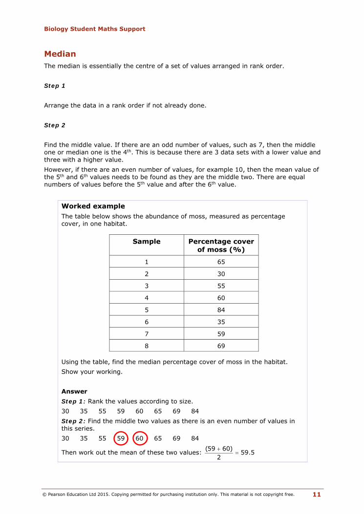
Median The median is essentially the centre of a set of values arranged in rank order. Step 1 Arrange the data in a rank order if not already done. Step 2 Find the middle value. If there are an odd number of values, such as 7, then the middle one or median one is the 4th. This is because there are 3 data sets with a lower value and three with a higher value. However, if there are an even number of values, for example 10, then the mean value of the 5th and 6th values needs to be found as they are the middle two. There are equal numbers of values before the 5th value and after the 6th value.

Worked example The table below shows the abundance of moss, measured as percentage cover, in one habitat. Using the table, find the median percentage cover of moss in the habitat. Show your working. Answer Step 1: Rank the values according to size. 30 35 55 59 60 65 69 84 Step 2: Find the middle two values as there is an even number of values in this series. 30 35 55 59 60 65 69 84

Then work out the mean of these two values: 5.592

)6059(

Sample Percentage cover of moss (%)

1 65

2 30

3 55

4 60

5 84

6 35

7 59

8 69



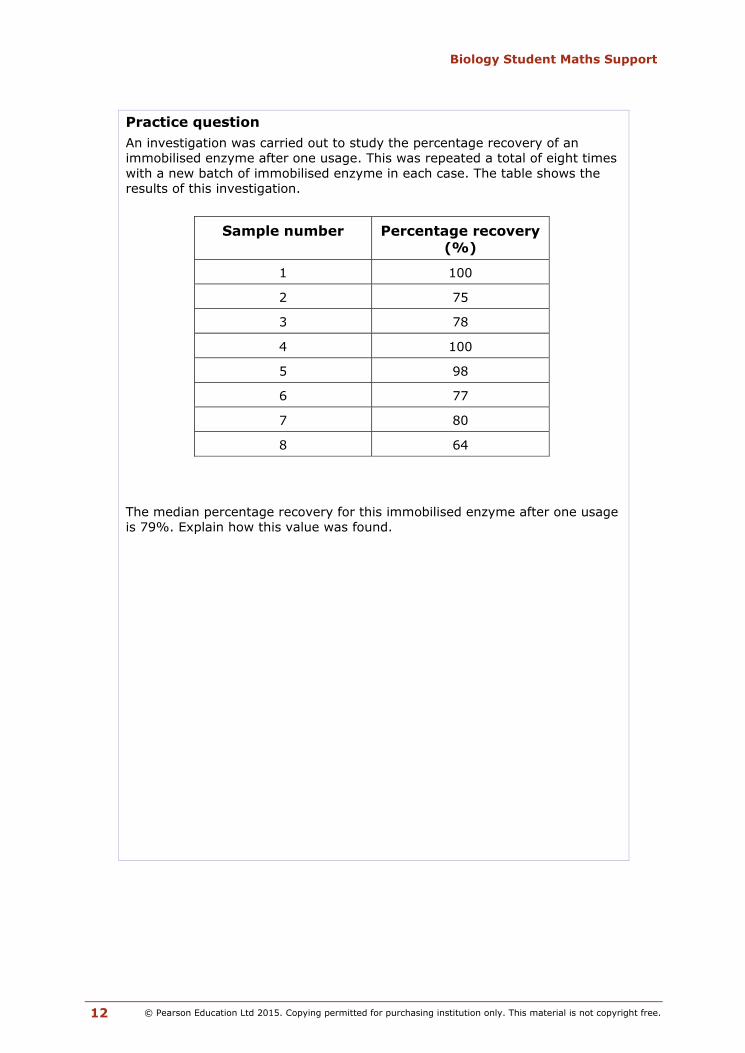
Practice question An investigation was carried out to study the percentage recovery of an immobilised enzyme after one usage. This was repeated a total of eight times with a new batch of immobilised enzyme in each case. The table shows the results of this investigation. The median percentage recovery for this immobilised enzyme after one usage is 79%. Explain how this value was found.

Sample number Percentage recovery (%)

1 100

2 75

3 78

4 100

5 98

6 77

7 80

8 64



Mode The mode is the most frequently occurring value in a series.

Worked example The table below shows some data relating to the ABO blood group alleles found in human populations on different islands. a Use this data to complete the table, by placing a tick in the box that

shows the allele with the mode for each island population. Answer If we consider Cuba, then the most common allele is O as between 90 and 100% of the population possess this allele. If we then look at the other islands, again the O allele is most common, though not as frequent as in Cuba. b Which of the three island populations has the mode for allele B? Answer This question asks for a study of the B allele row in the first table and identification of the country with a population showing the highest occurrence of this allele. The answer is Madagascar with a frequency of between 15 and 20% of the population. If only allele A is considered for populations found on Iceland, Madagascar and New Zealand, then all have the same level of occurrence. In this circumstance, there is no mode.

Allele

Frequency of allele occurrence

Cuba Iceland Madagascar New Zealand

A 0–5 15–20 15–20 15–20

B 0–5 5–10 15–20 5–10

O 90–100 70–80 60–70 70–80

Island population Allele A Allele B Allele O

Cuba

Iceland

Madagascar

New Zealand



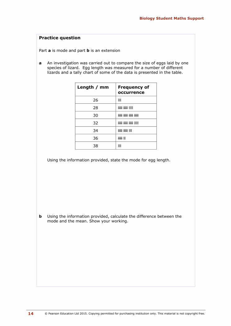
Practice question Part a is mode and part b is an extension a An investigation was carried out to compare the size of eggs laid by one

species of lizard. Egg length was measured for a number of different lizards and a tally chart of some of the data is presented in the table.

Using the information provided, state the mode for egg length. b Using the information provided, calculate the difference between the

mode and the mean. Show your working.

Length / mm Frequency of occurrence

26 III

28 IIII IIII IIII

30 IIII IIII IIII IIII

32 IIII IIII IIII IIII

34 IIII IIII III

36 IIII II

38 III



Temperature coefficient (Q10)

Q10 is the difference in the rate of an enzyme-controlled reaction as the temperature changes by 10°C, especially at temperatures below the optimum temperature. To calculate Q10 the following equation can be used.

Cat activity enzyme of rate

C10 at activity enzyme of rateQ

0

0

10 T

T

If the rate at T°C is 12 arbitrary units of product produced and at T + 10°C 22 units of product produced, then

83.11222Q10

This means that with this 10°C rise in temperature the enzyme produced 1.83 times as much product in the same time.

Worked example The graph below shows an enzyme-controlled reaction.

a Using the graph, calculate Q10 as the temperature increases from 20°C to

30°C. Show your working. Answer Rate of enzyme activity at 20°C is 13 au and at 30°C it is 24 au.

So 8.11324Q10

b What is Q10 if the temperature increases from 10°C to 20°C? A 2.0 B 2.2 C 2.4 D 2.6 Answer The answer is B. A common misconception is to simply divide 20°C by 10°C and produce an answer of 2.0, rather than finding the rate at each of these two temperatures.

If temperature T°C is 18°C, then T + 10°C is 28°C



Practice question If Q10 for enzyme E is 2.00, complete the table.

Temperature / °C

Enzyme E activity / arbitrary units

10 10

20

30

40



Productivity: GPP, NPP and R

Gross primary productivity (GPP), net primary productivity (NPP) and respiration (R) are all inter-related. They can be linked together using the following equation.

GPP = NPP + R Needless to say, it is quite possible that students would be given any two from the three components and be required to calculate the third. To do this, the equation may need to be rearranged. The following may help: 1 To calculate R use R = GPP – NPP 2 To calculate NPP use NPP = GPP – R If, for example, the GPP of an ecosystem is found to be 87 000 kJ m-2 year-1 and the respiration in the same ecosystem is 50 000 kJ m-2 year-1 then the NPP is:

NPP = 37 000 kJ m-2 year-1

Worked example A study was carried out to find the respiration per year in two different evergreen forests. To do this, scientists collected data on the NPP and GPP of the forests. The results are given in the table. Productivity is expressed here as grams of carbon fixed per square metre per year (g of C m-2 year-1). What is the respiration per year in the two different forests? Answer As the same process is being asked for both types of forest, the equation is

R = GPP – NPP So respiration per year for the broadleaf evergreen forest is

2700 – 1200 = 1500 g of C m-2 year-1 For the needle evergreen forest it is

820 – 440 = 380 g of C m-2 year-1

Type of evergreen forest

NPP / g of C m-2 year-1

GPP / g of C m-2 year-1

Broadleaf 1200 2700

Needle 440 820



Practice question 1 The ratio of NPP : GPP can be used by scientists when studying productivity in different types of land. Use the data below to work out the NPP : GPP ratio for these two types of land. Grassland data: GPP = 400 g of C m-2 year-1 and R = 140 g of C m-2 year-1 Scrubland data: NPP = 230 g of C m-2 year-1 and R = 130 g of C m-2 year-1

Practice question 2 The graph shows the GPP and NPP for two types of savannah, woody and non-woody.

Using the graph, calculate the difference in the respiration per year between the two different types of savannah. Show your working.



Animal population estimation: Lincoln Index

The Lincoln Index is a type of mark recapture technique used to estimate the population size of mobile animals. All the animals collected on one occasion are marked and counted (M1). After an appropriate time, another collection in the same area is carried out and the number of animals caught is found (T). Also the number of marked individuals in this second collection are counted (M2). To estimate the population of this animal the following equation can be used.

8.1)(

population Total2

1

M

TM

So if M1 = 50, M2 = 15 and T = 300 then the total population is

15)30050( =

1515000 = 1000 individuals

Worked example A student wished to estimate the number of one species of aquatic snail in a pond. She collected 110 on day 1 and marked the shell of them all with a small spot of waterproof paint. On day 2 she collected all the snails she could find. She found 35 with paint on them and 230 without. Calculate the population size in the pond for this species. Answer M1 = 110, M2 = 35 and T = 230

Her population size was 35

)265110( = 833 snails

Practice question A study was carried out to consider whether the population size of a malarial mosquito changed between the dry season and the wet season in Africa. The student performed a mark recapture technique in the same area in the dry season and in the wet season of the same year. The results of her study are shown in the table. Using the data provided, state whether the population was increasing or decreasing between the dry season and the wet season. Give reasons for your answer.

Season Number marked

Number recaptured

Number recaptured with mark on

Dry 88 89 4

Wet 175 227 4



Habitat biodiversity using an index of diversity (D)

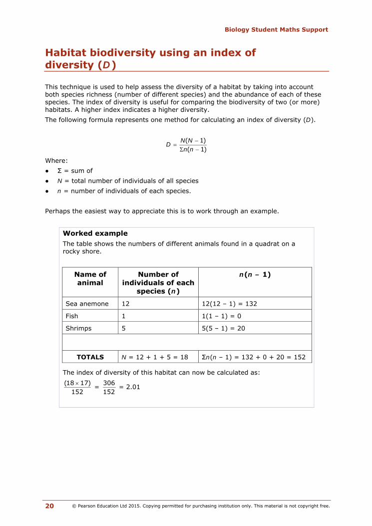
This technique is used to help assess the diversity of a habitat by taking into account both species richness (number of different species) and the abundance of each of these species. The index of diversity is useful for comparing the biodiversity of two (or more) habitats. A higher index indicates a higher diversity. The following formula represents one method for calculating an index of diversity (D).

)1()1(

nnNND

Where: ● Σ = sum of ● N = total number of individuals of all species ● n = number of individuals of each species. Perhaps the easiest way to appreciate this is to work through an example.

Worked example The table shows the numbers of different animals found in a quadrat on a rocky shore. The index of diversity of this habitat can now be calculated as:

152)1718( =

152306 = 2.01

Name of animal

Number of individuals of each

species (n)

n(n – 1)

Sea anemone 12 12(12 – 1) = 132

Fish 1 1(1 – 1) = 0

Shrimps 5 5(5 – 1) = 20

TOTALS N = 12 + 1 + 5 = 18 Σn(n – 1) = 132 + 0 + 20 = 152



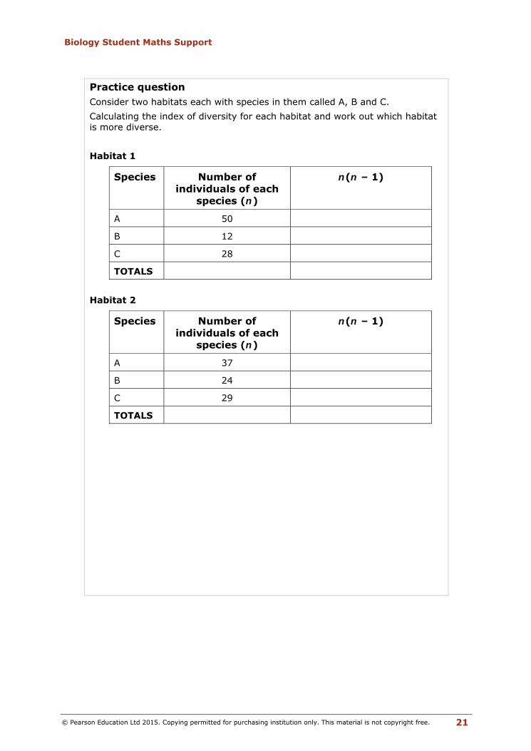
Practice question Consider two habitats each with species in them called A, B and C. Calculating the index of diversity for each habitat and work out which habitat is more diverse. Habitat 1 Habitat 2

Species Number of individuals of each

species (n)

n(n – 1)

A 50

B 12

C 28

TOTALS

Species Number of individuals of each

species (n)

n(n – 1)

A 37

B 24

C 29

TOTALS



The Hardy–Weinberg principle

The Hardy–Weinberg principle is used in population genetics to calculate the frequency of alleles and genotypes. For a population to be in equilibrium the following conditions must be satisfied: ● the population is large ● random breeding ● no mutations ● no selection ● no migration into or out of the population. The Hardy–Weinberg principle applies to monohybrid inheritance, where a character is controlled by a single gene (e.g. A). The genotypes in this population would, therefore, be AA, Aa and aa. We use the following two equations to calculate the allele and genotype frequencies:

p + q = 1 (or 100% of the population) [equation 1] where p represents the frequency of the allele A and q represents the frequency of the allele a and

p2 + 2pq + q2 = 1 (or 100% of the population) [equation 2] where p2 represents the frequency of the genotype AA, 2pq represents the frequency of the genotype Aa and q2 represents the frequency of the genotype aa.

Worked example In tobacco plants, the production of chlorophyll is controlled by a single allele, A. Seedlings with the genotype aa lack chlorophyll and die soon after germination. In a sample of 600 seedlings, 132 lacked chlorophyll. Calculate the expected number of heterozygous seedlings in this sample. Answer From these results, we know that the frequency of seedlings with the genotype aa is 0.22 (22%) This represents q2 in equation 2, so the frequency of the allele a is:

22.0 = 0.469 (= q)

We can now find the frequency of the allele A, using equation 1: 1 – 0.469 = 0.531 (= p)

We now know the values of p (0.531) and q (0.469), so using equation 2, the frequency of heterozygotes is:

2pq = 2 × 0.531 × 0.469 = 0.498 This represents 49.8% of the total number of seedlings, that is, 49.8% of 600 which is 299 seedlings (rounded up to the nearest whole number).



Practice question In fruit flies, wing length is controlled by a single gene. Fruit flies with the homozygous recessive genotype have short wings. In a sample of 350 fruit flies, 73 were found to have short wings. Use the Hardy-Weinberg principle to calculate the expected number of fruit flies in this sample with the homozygous dominant genotype.



Standard deviation

The standard deviation gives a measure of the spread of a normal distribution around the mean value. If the data are tightly clustered around the mean, the standard deviation will be small. If the data are more widely spread, then the standard deviation will be larger. The following formula is usually used to calculate the standard deviation:

1

)( 22

n

nXX

S

Where: ● S is the standard deviation ● ∑ = sum of ● X = each measurement (e.g. width or mass) ● n = the total number of measurements. This is known as the ‘sample standard deviation’ and is used when taking a sample from a much larger population.

Worked example The table shows the lengths of a sample of 20 mollusc shells. Calculate the standard deviation for this sample. Answer Step 1: calculate X2 values. Step 2: find ∑X and ∑X2. Step 3: substitute values into the formula to find S. S = 1.06

Mollusc shell length / cm (X) X2

1 3.2 10.24 2 5.1 26.01 3 2.6 6.76 4 4.6 21.16 5 3.8 14.44 6 6.5 42.25 7 5.0 25.0 8 3.6 12.96 9 6.9 47.61 10 4.8 23.04 11 4.6 21.16 12 4.4 19.36 13 4.0 16.0 14 4.4 19.36 15 4.8 23.04 16 5.9 34.81 17 6.0 36.0 18 4.9 24.01 19 4.4 19.36 20 5.2 27.04

Totals (∑) 94.7 469.61



Practice question The table shows the number of snails found in 10 quadrats. Each quadrat measured 1 m × 1 m. a Calculate the mean number of snails per quadrat. b Calculate the standard deviation for this sample.

Quadrat number Number of snails found in each quadrat

1 14

2 15

3 14

4 16

5 12

6 14

7 14

8 12

9 16

10 13



Statistics

Students are expected to know three statistical tests: ● the Chi-squared (2) test ● the Student’s t-test ● the correlation coefficient.

The Chi-squared test

This is also sometimes referred to as the ‘goodness of fit’ test and is used to see how closely experimental results fit expected results. It is particularly useful in genetics, where the expected results can be predicted using Mendelian ratios, such as 9 : 3 : 3 : 1, or 1 : 1. The Chi-squared test can also be used in choice chamber experiments, or prey selection, such as different coloured snail shells selected by thrushes. The formula for the Chi-squared test is as follows:

EEO 2

2 )(

Where: ● 2 is the Chi-squared value ● ∑ = sum of ● O = the observed values ● E = the expected values.



Worked example A breeding experiment was carried out using fruit flies. The table shows the results of this experiment. Use a Chi-squared test to investigate whether these results fit the expected 9 : 3 : 3 : 1 ratio for a cross involving unlinked genes. Answer Step 1: Calculate the expected numbers (E) of each phenotype, using the expected 9 : 3 : 3 : 1 ratio. The total number of flies in this sample is 128, therefore the expected number of flies with the phenotype long wings and wild-type body colour will be

816128

× 9 = 72 (from the ratio parts, 9 + 3 + 3 + 1 = 16)

Step 2: Calculate the difference between each pair of observed and expected numbers (O – E). Step 3: Square each of these values to obtain (O – E)2. Step 4: Divide the (O – E)2 values by the expected numbers (E). Step 5: Add these to find the Chi-squared value. These steps are shown in the following table.

Phenotype long wings

and wild-type body colour

long wings and black

body colour

vestigial wings and wild-type

body colour

vestigial wings and black body

colour

Observed numbers (O)

76 21 26 5

Phenotype long wings

and wild-type body colour

long wings and black

body colour

vestigial wings and wild-type

body colour

vestigial wings and black body

colour

Observed numbers (O)

76 21 26 5

Expected numbers (E)

72 24 24 8

O – E 4 -3 2 -3

(O – E)2 16 9 4 9

(O – E)2 ÷ E

0.22 0.38 0.17 1.13

Total 0.22 + 0.38 + 0.17 + 1.13 = 1.9



Interpreting the results of the Chi-squared test. The larger the value of Chi-squared, the more certain we can be that there is a difference between the observed and expected results. We need to compare the calculated value of Chi-squared with the critical value at p = 0.05 (or 5%) for the appropriate number of degrees of freedom. In this case, with one row of data, the number of degrees of freedom (df) = the number of columns – 1, i.e. df = 4 – 1 = 3. Here is a table of critical values for the Chi-squared test.

Degrees of freedom

(df)

Levels of significance (p)

0.05 0.025 0.01 0.005 0.001

1 3.84 5.02 6.63 7.88 10.83

2 5.99 7.38 9.21 10.60 13.81

3 7.81 9.35 11.34 12.84 16.27

4 9.49 11.14 13.28 14.86 18.47

The calculated value for Chi-squared (1.9) is less than the critical value at p = 0.05 for 3 degrees of freedom, so the results of this breeding experiment are in the ratio of 9 : 3 : 3 : 1.

Practice question A test cross was carried out between two maize plants, one with yellow, smooth cobs and the other with white, wrinkled cobs. The table shows the results of this cross. Use a Chi-squared test to investigate whether these results fit the expected 1 : 1 : 1 : 1 ratio.

Type of maize cob

yellow and smooth

yellow and wrinkled

white and smooth

white and wrinkled

Number of cobs 28 33 30 34



The Student’s t-test

This test is used to compare the means of two sets of data, if the data are normally distributed. For example, we could use the t-test to investigate whether the difference between the mean width of shade leaves is significantly different from the mean width of sun leaves. Incidentally, this test is not named as such because it is widely used by students, but because ‘Student’ was the pen-name of William Sealy Gosset, who introduced the test in 1908. The formula for Student’s t-test is as follows.

2

22

1

21

21t

NS

NS

xx

Where

● 1x = the mean of the first set of data

● 2x = the mean of the second set of data

● S1 = the standard deviation of the first set of data ● S2 = the standard deviation of the second set of data ● N1 = the number of measurements in the first set of data ● N2 = the number of measurements in the second set of data Calculations of mean and standard deviation are explained on pages 9 and 24



Worked example An investigation was carried out to compare the shell lengths of a species of mollusc from two sites, A and B. Ten specimens were collected at random from each site and length of each shell was measured and recorded. The table below shows the results of this investigation. a Calculate the mean shell length for Site B. Answer The mean shell length for Site B is 26.3 mm b Using the formula for Student’s t-test, calculate the value of t for these

results. Answer Step 1: Calculate the difference between the means. Step 2: Square each of the standard deviations. Divide S2 by N for both sets of data and add together. Step 3: Find the square root of the total from Step 2. Step 4: Divide the difference between the means by the square root from Step 3, to find the t value. Note: if the t value is negative, ignore the minus sign to convert it to a positive number. In this example, t = 6.85.

Shell lengths / mm

Site A Site B

35 15

70 18

45 19

50 23

55 26

60 27

64 32

68 34

62 29

78 40

Mean for Site A = 58.7 Mean for Site B =

Standard deviation for Site A = 12.76

Standard deviation for Site B = 7.80



Interpreting the results of the t-test. We need to compare the t-value with the critical value at p = 0.05 (or 5%) for the appropriate number of degrees of freedom (df). Calculate the number of degrees of freedom, using the following formula.

df = N1 + N2 – 2 In this example, df = 10 + 10 – 2 = 18 Here is an extract from a table of critical values for a t-test, with 18 degrees of freedom.

Degrees of

freedom (df)

Levels of significance (p)

0.05 0.02 0.01 0.002 0.001

18 2.101 2.552 2.878 3.610 3.922 The calculated value of t (6.85) is greater than the critical value at p = 0.05 (2.101), so we can say that the difference between the means is significant.



Practice question Dog’s mercury is a plant that grows in shady areas in woodland and in open clearings. An investigation was carried out to determine whether there was a significant difference between the surface area of the leaves from dog’s mercury plants growing in the shaded areas and open clearings of a wood. Seventeen leaves of dog’s mercury were collected from plants growing in a shaded area (Site A) and seventeen leaves were also collected from plants growing in an open clearing (Site B). The surface area of each leaf was measured. The table shows the results of this investigation. a Calculate the mean surface area of the leaves from Site B. b State the number of degrees of freedom for this investigation. c A statistical table showed that the critical value at p = 0.05 is 2.04. Use Student’s t-test to determine whether the difference in mean surface

area is significant.

Surface area of leaves / cm2

Shaded area (Site A) Open clearing (Site B) 21 15 14 17 16 18 18 17 19 17 21 19 19 13 22 14 18 21 16 13 13 16 22 13 21 16 23 12 19 14 18 12 15 20

Mean for Site A = 18.53 Mean for Site B = Standard deviation for Site A = 2.87

Standard deviation of Site B = 2.70



Correlation coefficient

The correlation coefficient is used to test the strength of the relationship between two variables. The correlation coefficient can vary from – 1, through 0, to +1. A correlation coefficient of -1 indicates a perfect negative correlation and a coefficient of +1 indicates a perfect positive correlation. A correlation coefficient of 0 indicates that there is no relationship between the two variables. One correlation test is known as Spearman’s rank correlation test. This is used to test the relationship between two variables, where the data are not normally distributed. The formula for Spearman’s rank correlation test is as follows.

)1()(61

2

2

nndrs

Where: ● rs = the correlation coefficient ● ∑ = sum of ● d = the difference between each pair of ranks (explained in the worked example) ● n = the size of the sample (number of pairs of values) Note: n(n2 – 1) is sometimes written as n3 – n.



Worked example An investigation was carried out into the relationship between the soil moisture content and the number of reed plants growing in the soil. Eleven samples were taken and the number of reed plants were counted, using a 0.25 m2 quadrat. The soil moisture content of each sample, expressed as a percentage, was also determined. The results are shown in the table below. It is a good idea to start by plotting a scatter diagram to see if there is any relationship between these two variables.

The scatter diagram shows a relationship between the variables; overall, as the soil moisture content increases, the number of reed plants per quadrat also increases.

contd.

Sample 1 2 3 4 5 6 7 8 9 10 11

Number of reed plants per quadrat

11 15 10 12 5 0 8 16 7 13 14

Soil moisture content (%)

23 28 18 27 10 7 14 30 8 15 25



Step 1 Rank the data in each set, so that the highest value is given the ranking ‘1’, the second highest value is given the ranking ‘2’ and so on. If two values are the same (tied numbers) they are each given the mean rank. Step 2 Find the differences (d) between each pair of ranks. For example, for the first pair of measurements, d = 6 – 5 = 1. Add another row to the table for these d values. Step 3 Square the d values. Add another row to the table for these d2 values.

contd.

Sample 1 2 3 4 5 6 7 8 9 10 11


11 15 10 12 5 0 8 16 7 13 14

Rank 6 2 7 5 10 11 8 1 9 4 3


23 28 18 27 10 7 14 30 8 15 25

Rank 5 2 6 3 9 10 8 1 11 7 4

Sample 1 2 3 4 5 6 7 8 9 10 11


11 15 10 12 5 0 8 16 7 13 14

Rank 6 2 7 5 10 11 8 1 9 4 3


23 28 18 27 10 7 14 30 8 15 25

Rank 5 2 6 3 9 10 8 1 11 7 4

d 1 0 1 2 1 1 0 0 -2 -3 -1

Sample 1 2 3 4 5 6 7 8 9 10 11


11 15 10 12 5 0 8 16 7 13 14

Rank 6 2 7 5 10 11 8 1 9 4 3


23 28 18 27 10 7 14 30 8 15 25

Rank 5 2 6 3 9 10 8 1 11 7 4

d 1 0 1 2 1 1 0 0 -2 -3 -1

d2 1 0 1 4 1 1 0 0 4 9 1



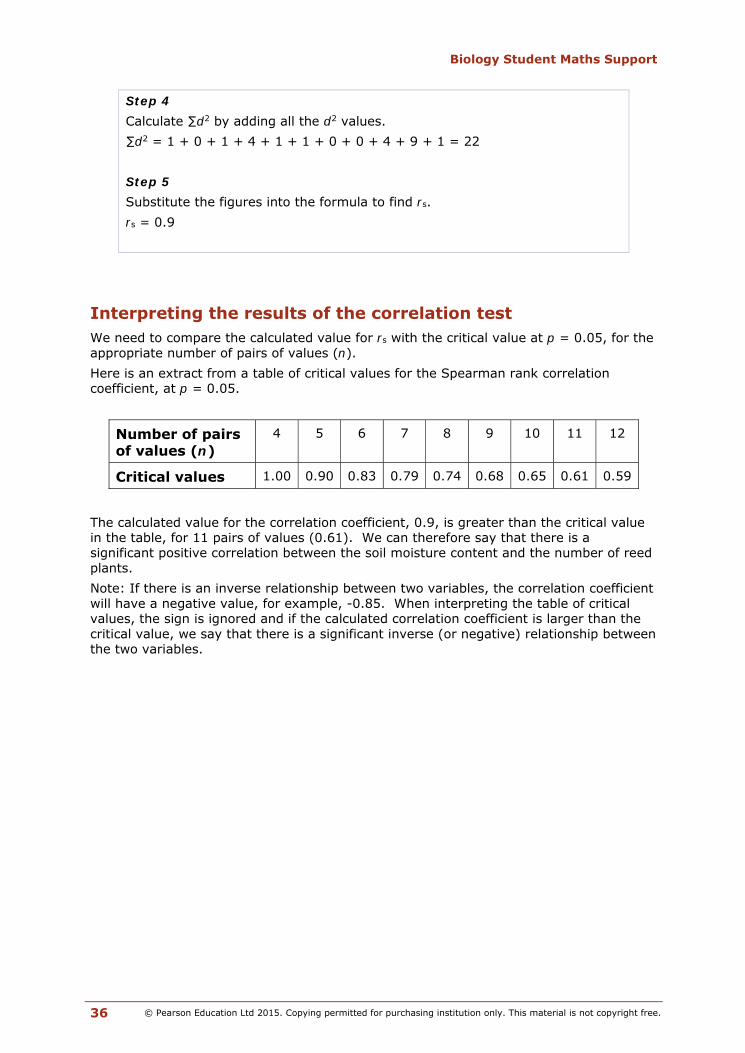
Step 4 Calculate ∑d2 by adding all the d2 values. ∑d2 = 1 + 0 + 1 + 4 + 1 + 1 + 0 + 0 + 4 + 9 + 1 = 22 Step 5 Substitute the figures into the formula to find rs. rs = 0.9

Interpreting the results of the correlation test We need to compare the calculated value for rs with the critical value at p = 0.05, for the appropriate number of pairs of values (n). Here is an extract from a table of critical values for the Spearman rank correlation coefficient, at p = 0.05.

Number of pairs of values (n)

4 5 6 7 8 9 10 11 12

Critical values 1.00 0.90 0.83 0.79 0.74 0.68 0.65 0.61 0.59

The calculated value for the correlation coefficient, 0.9, is greater than the critical value in the table, for 11 pairs of values (0.61). We can therefore say that there is a significant positive correlation between the soil moisture content and the number of reed plants. Note: If there is an inverse relationship between two variables, the correlation coefficient will have a negative value, for example, -0.85. When interpreting the table of critical values, the sign is ignored and if the calculated correlation coefficient is larger than the critical value, we say that there is a significant inverse (or negative) relationship between the two variables.



Practice question An investigation was carried out into the relationship between length and mass in a species of tuna, caught in the Pacific Ocean. Twelve specimens were caught and the length and mass of each fish was recorded. The table below shows the results of this investigation. a Plot a scatter diagram of the data and describe the relationship. b Calculate the Spearman’s rank correlation coefficient for the data. c What does your calculated value indicate about the relationship between

these two variables?

Fish number 1 2 3 4 5 6 7 8 9 10 11 12

Length / cm 100 112 130 143 103 98 93 118 140 138 122 82

Mass / kg 56 45 62 50 27 16 32 54 80 60 38 20



Further questions

Question 1 Ultraviolet light (UV) can be used to kill microorganisms. A student carried out an investigation into the effect of UV light on the survival of bacteria. The student spread bacteria evenly on three agar plates. Each plate was then exposed to UV light for one minute. The student then placed the agar plates in an incubator. The procedure was repeated for exposure times of 2, 3, 4 and 5 minutes. After 48 hours, the number of bacterial colonies on each plate were recorded. The results are shown below. a Write a suitable null hypothesis for this investigation. b Complete the following table, by calculating the mean number of bacterial

colonies for each UV exposure time.

contd.

Exposure time / min

Number of bacterial colonies

1 302 282 322

2 187 215 231

3 174 108 129

4 70 94 82

5 37 47 21

Exposure time / min Mean number of bacterial colonies

1

2

3

4

5



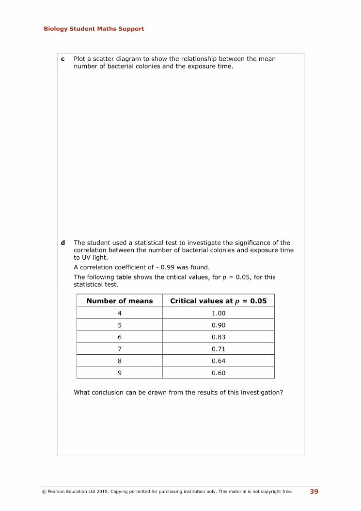
c Plot a scatter diagram to show the relationship between the mean number of bacterial colonies and the exposure time.

d The student used a statistical test to investigate the significance of the

correlation between the number of bacterial colonies and exposure time to UV light.

A correlation coefficient of - 0.99 was found. The following table shows the critical values, for p = 0.05, for this

statistical test. What conclusion can be drawn from the results of this investigation?

Number of means Critical values at p = 0.05

4 1.00

5 0.90

6 0.83

7 0.71

8 0.64

9 0.60



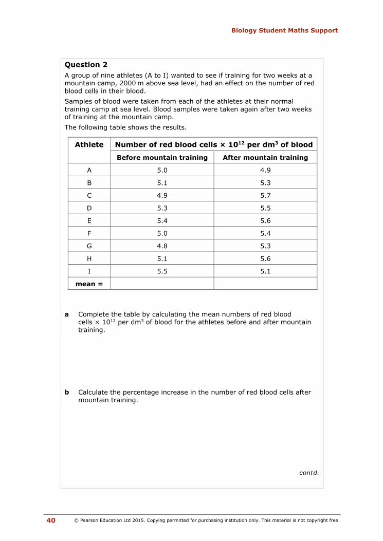
Question 2 A group of nine athletes (A to I) wanted to see if training for two weeks at a mountain camp, 2000 m above sea level, had an effect on the number of red blood cells in their blood. Samples of blood were taken from each of the athletes at their normal training camp at sea level. Blood samples were taken again after two weeks of training at the mountain camp. The following table shows the results. a Complete the table by calculating the mean numbers of red blood

cells × 1012 per dm3 of blood for the athletes before and after mountain training.

b Calculate the percentage increase in the number of red blood cells after

mountain training.

contd.

Athlete Number of red blood cells × 1012 per dm3 of blood

Before mountain training After mountain training

A 5.0 4.9

B 5.1 5.3

C 4.9 5.7

D 5.3 5.5

E 5.4 5.6

F 5.0 5.4

G 4.8 5.3

H 5.1 5.6

I 5.5 5.1

mean =



c Write a null hypothesis for this investigation. d A Student’s t-test was applied to the data to test the null hypothesis. i State the number of degrees of freedom for these results. ii The calculated value of t was found to be 2.24. The following table gives critical values of t, for the appropriate

number of degrees of freedom. What conclusion can be drawn from the results of this investigation?

Significance level (p) 0.20 0.10 0.05 0.01 0.001

Critical value of t 1.34 1.75 2.12 2.92 4.02



Checklist of mathematical skills

Mathematical skills

I am confident with these skills ()

Recognise and make use of appropriate units in calculations

Recognise and use expressions in decimal and standard form

Use ratios, fractions and percentages

Estimate results

Use calculators to find and use power, exponential and logarithmic functions (A level only)

Use an appropriate number of significant figures

Find arithmetic means

Construct and interpret frequency tables and diagrams, bar charts and histograms

Understand simple probability

Understand the terms mean, median and mode

Use a scatter diagram to identify a correlation between two variables

Make order of magnitude calculations

Select and use a statistical test

Understand measures of dispersion, including standard deviation and range

Identify uncertainties in measurements and use simple techniques to determine uncertainty when data are combined

Understand and use the symbols: =, <, <<, >>, >, , ~

Change the subject of an equation

Substitute numerical values into algebraic equations using appropriate units for physical quantities

Solve algebraic equations

Use logarithms in relations to quantities that range over several orders of magnitude (A level only)

Translate information between graphical, numerical and algebraic forms

Plot two variables from experimental or other data

Understand that y = mx + c represents a linear relationship

Determine the intercept of a graph (A level only)

Calculate rate of change from a graph showing a linear relationship

Draw and use the slope of a tangent to a curve as a measure of rate of change

Calculate the circumferences, surfaces areas and volumes of regular shapes

as and a level biology - pearson qualifications level/biology... · mathematical skills are an...

Documents