as the deer pants for streams of water, so my soul pants...
TRANSCRIPT

As the deer pants for streams of water, so my soul pants for you, O God.
Psalm 42:1
My people have committed two sins: They have forsaken me, the spring of living
water, and have dug their own cisterns, broken cisterns that cannot hold water.
Jer 2:13
Welcome to Programming Languages (ITP20005)
No more labs: • All Labs and Discussions with solutions are available from www.cs61a.org,
CS61A course Fall 2014.• They are the best resources for your mid term exam. • Some problems and answers of our labs and homework are searchable in the
web ^^, such as Hanoi Tower, Church Numerals and so on. • I will try to avoid it for your homework, we cannot avoid some of them since
we have to know those well known questions too.
No more labs, but homework • Homework 03 – Recursion• Due is 09:59 am on Oct.13, 2014• Don’t forget running a doctest and including docstring in every function.
If there is no docstring, you should provide it. If there are errors in docstring, you should fix them. It is a required part of your homework. That counts -0.2 and it matters.
Welcome to Programming Languages (ITP20005)
Hog Project (10 points) – Due: Oct. 6, Extended to Oct. 10, 10:10 PM • It will take your time, at least 16 hours – two full days long.
Not familiar with Python? it may take much longer.• The project concept video available from
login: pl20005 password: pl20005.• Refer to www.cs61a.org, but look for hog project Summer 2014
CS61A course, not Fall 2014.• Two of you can work together – no penalty, but each one of you
must understand the concept and programming.You are encouraged to do it by yourself, and to help each other verbally or debugging when you are stuck on a certain problem. But, never give a piece of your code in paper or in file.
• When two of you decide to work together, declare your partner's name and describe each's roles in detail at the beginning of hog project file hog.py.
ITP 20005 Programming LanguagesChapter 1 & 3 • Lambda Calculus
Prof. Youngsup Kim, [email protected], 2014 Programming Languages, CSEE Dept., Handong Global University
5
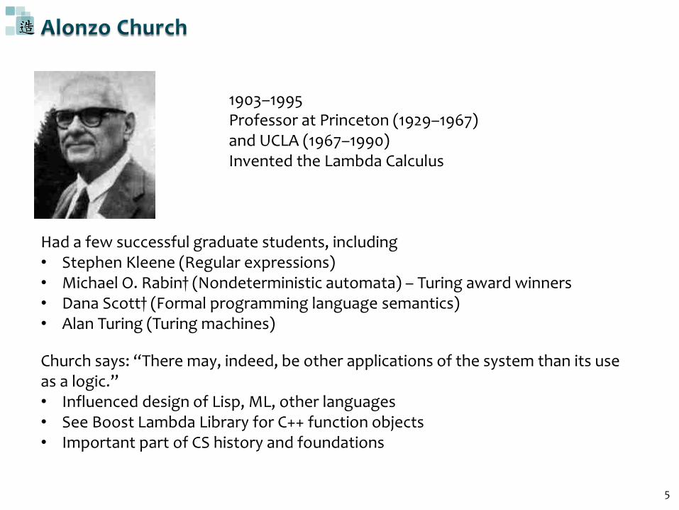
Had a few successful graduate students, including• Stephen Kleene (Regular expressions)• Michael O. Rabin† (Nondeterministic automata) – Turing award winners• Dana Scott† (Formal programming language semantics)• Alan Turing (Turing machines)
1903–1995Professor at Princeton (1929–1967)and UCLA (1967–1990)Invented the Lambda Calculus
Church says: “There may, indeed, be other applications of the system than its use as a logic.”• Influenced design of Lisp, ML, other languages• See Boost Lambda Library for C++ function objects• Important part of CS history and foundations
6
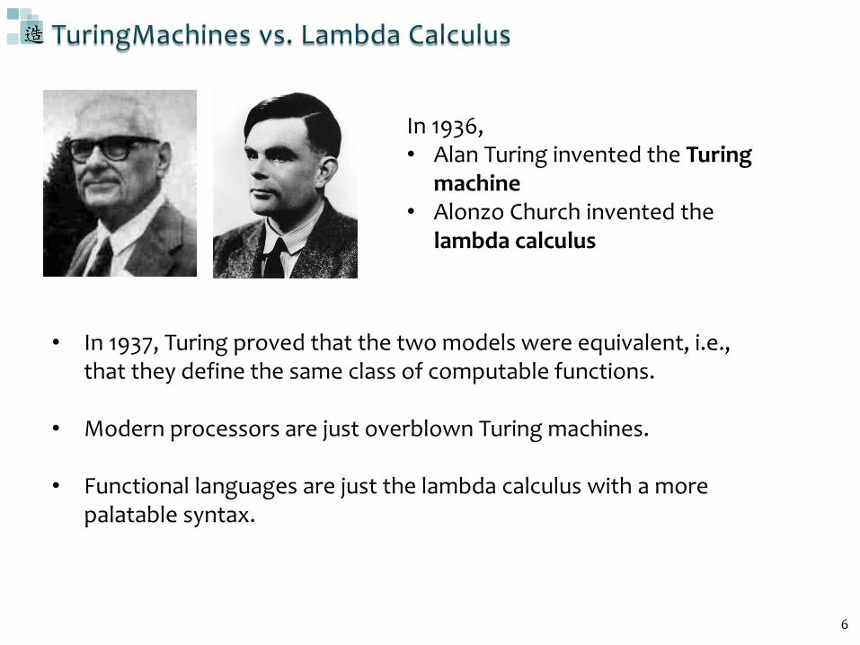
• In 1937, Turing proved that the two models were equivalent, i.e., that they define the same class of computable functions.
• Modern processors are just overblown Turing machines.
• Functional languages are just the lambda calculus with a more palatable syntax.
In 1936,• Alan Turing invented the Turing
machine• Alonzo Church invented the
lambda calculus
Essentially every full-scale programming language has some notion of function.
The (pure) lambda calculus is a language composed entirely of functions.
We use the lambda calculus to study the essence of computation.
It is just as fundamental as Turing Machines.
Lisp originally departed from standard lambda calculus, returned to the fold through Scheme, Common Lisp
8
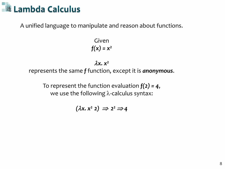
A unified language to manipulate and reason about functions.
Givenf(x) = x2
x. x2
represents the same f function, except it is anonymous.
To represent the function evaluation f(2) = 4, we use the following -calculus syntax:
(x. x2 2) 22 4
9
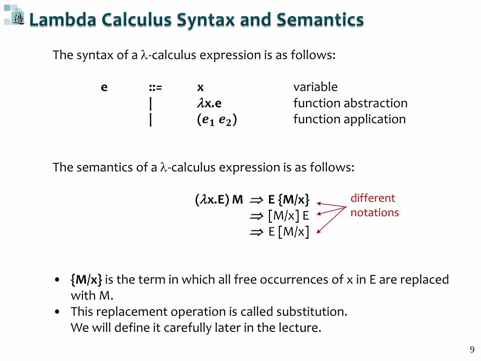
The syntax of a -calculus expression is as follows:
e ::= x variable| x.e function abstraction| (𝒆𝟏 𝒆𝟐) function application
The semantics of a -calculus expression is as follows:
(x.E) M E {M/x} [M/x] E E [M/x]
• {M/x} is the term in which all free occurrences of x in E are replaced with M.
• This replacement operation is called substitution. We will define it carefully later in the lecture.
different notations
6.10
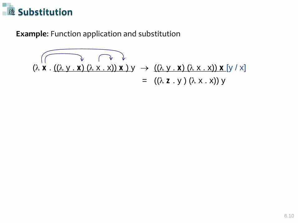
( x . (( y . x) ( x . x)) x ) y (( y . x) ( x . x)) x [y / x]
= (( z . y ) ( x . x)) y
Example: Function application and substitution
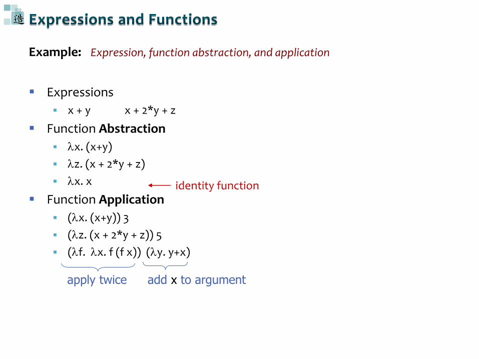
Expressions
x + y x + 2*y + z
Function Abstraction
x. (x+y)
z. (x + 2*y + z)
x. x
Function Application
(x. (x+y)) 3
(z. (x + 2*y + z)) 5
(f. x. f (f x)) (y. y+x)
Example: Expression, function abstraction, and application
identity function
apply twice add x to argument
6.12
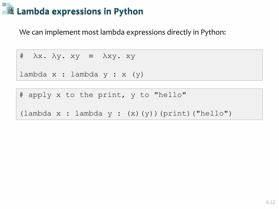
We can implement most lambda expressions directly in Python:
# λx. λy. xy λxy. xy
lambda x : lambda y : x (y)
# apply x to the print, y to "hello"
(lambda x : lambda y : (x)(y))(print)("hello")
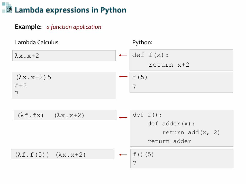
Example: a function application
def f(x):
return x+2
Python:
f(5)
7
Lambda Calculus
x.x+2
(x.x+2)5
5+2
7
(f.fx) (x.x+2)
(f.f(5)) (x.x+2)
def f():
def adder(x):
return add(x, 2)
return adder
f()(5)
7
6.14
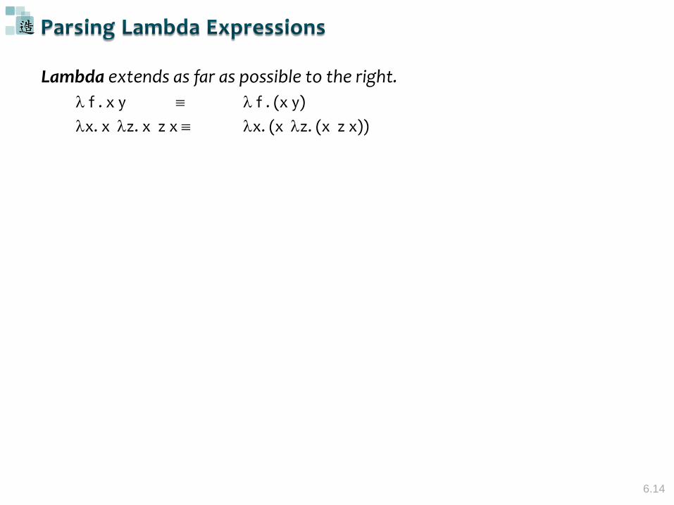
Lambda extends as far as possible to the right.
f . x y f . (x y)
x. x z. x z x x. (x z. (x z x))
6.15
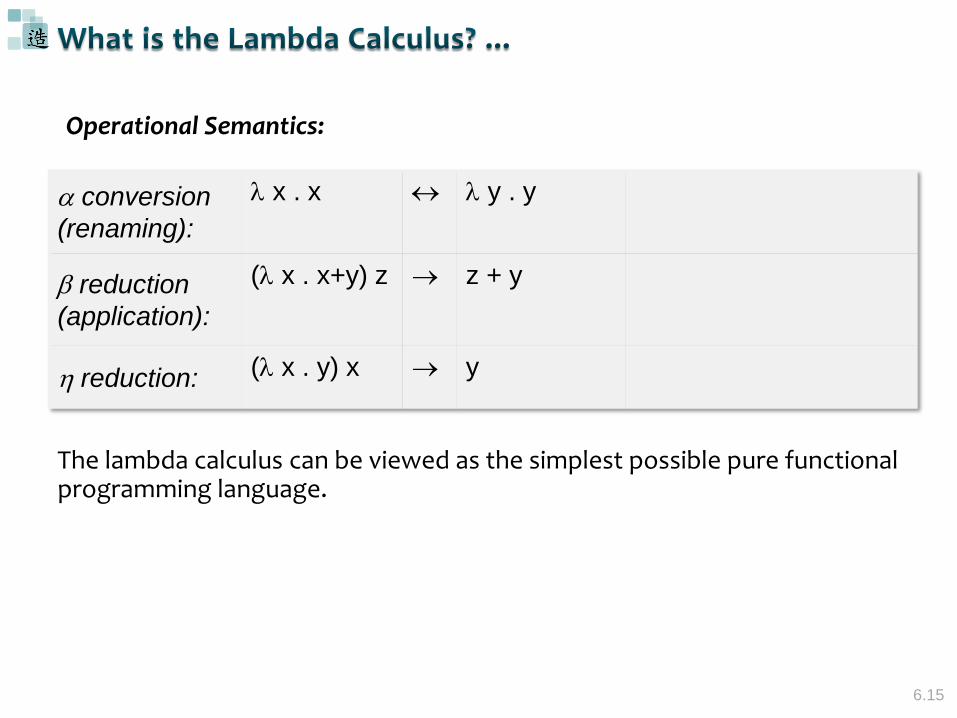
Operational Semantics:
The lambda calculus can be viewed as the simplest possible pure functional programming language.
conversion
(renaming):
x . x y . y
reduction
(application):
( x . x+y) z z + y
reduction: ( x . y) x y
6.16
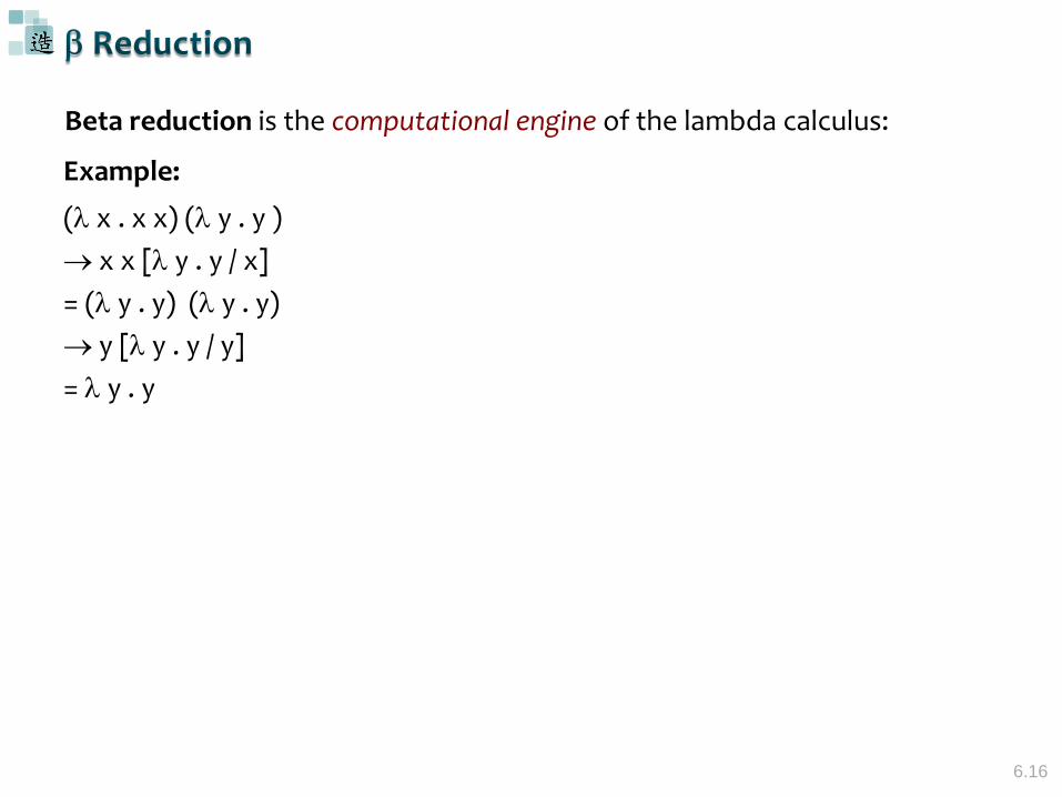
Beta reduction is the computational engine of the lambda calculus:
( x . x x) ( y . y )
x x [ y . y / x]
= ( y . y) ( y . y)
y [ y . y / y]
= y . y
Example:
6.17
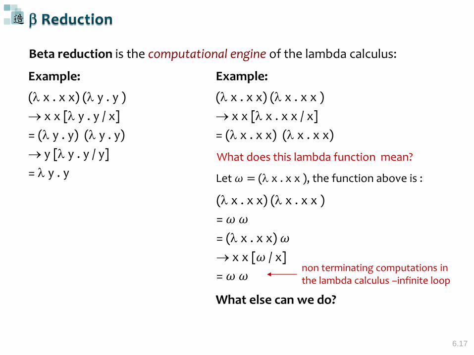
Beta reduction is the computational engine of the lambda calculus:
( x . x x) ( y . y )
x x [ y . y / x]
= ( y . y) ( y . y)
y [ y . y / y]
= y . y
Example:
( x . x x) ( x . x x )
x x [ x . x x / x]
= ( x . x x) ( x . x x)
Example:
What does this lambda function mean?
Let 𝜔 = ( x . x x ), the function above is :
( x . x x) ( x . x x )
= 𝜔 𝜔
= ( x . x x) 𝜔
x x [𝜔 / x]
= 𝜔 𝜔non terminating computations in the lambda calculus –infinite loop
What else can we do?
6.18
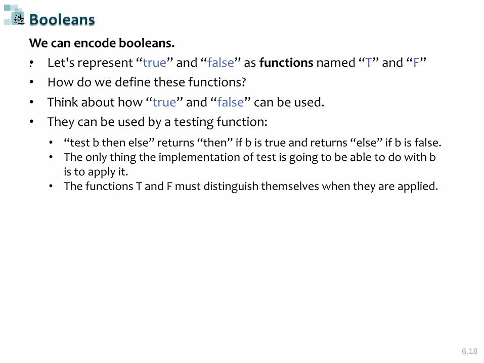
We can encode booleans.
.• Let's represent “true” and “false” as functions named “T” and “F”
• How do we define these functions?
• Think about how “true” and “false” can be used.
• They can be used by a testing function:
• “test b then else” returns “then” if b is true and returns “else” if b is false.• The only thing the implementation of test is going to be able to do with b
is to apply it.• The functions T and F must distinguish themselves when they are applied.
6.19
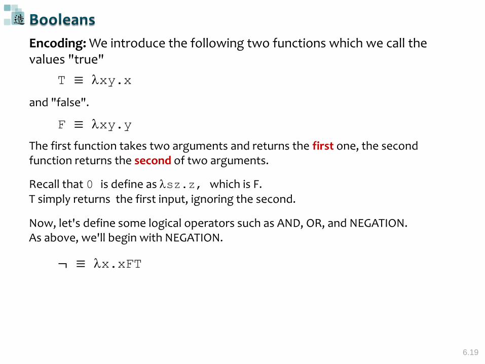
Encoding: We introduce the following two functions which we call the values "true"
T ≡ xy.x
F ≡ xy.y
and "false".
The first function takes two arguments and returns the first one, the second function returns the second of two arguments.
Recall that 0 is define as sz.z, which is F. T simply returns the first input, ignoring the second.
Now, let's define some logical operators such as AND, OR, and NEGATION.As above, we'll begin with NEGATION.
¬ ≡ x.xFT
6.20
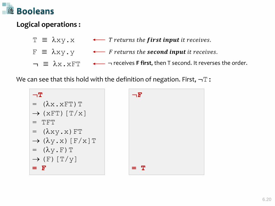
Logical operations :
T ≡ xy.x
F ≡ xy.y
We can see that this hold with the definition of negation. First, ¬T:
¬ ≡ x.xFT
¬T= (x.xFT)T
(xFT)[T/x]
= TFT
= (xy.x)FT
(y.x)[F/x]T
= (y.F)T
(F)[T/y]
= F
¬F
= T
¬ receives F first, then T second. It reverses the order.
𝑇 𝑟𝑒𝑡𝑢𝑟𝑛𝑠 𝑡ℎ𝑒 𝒇𝒊𝒓𝒔𝒕 𝒊𝒏𝒑𝒖𝒕 𝑖𝑡 𝑟𝑒𝑐𝑒𝑖𝑣𝑒𝑠.
𝐹 𝑟𝑒𝑡𝑢𝑟𝑛𝑠 𝑡ℎ𝑒 𝒔𝒆𝒄𝒐𝒏𝒅 𝒊𝒏𝒑𝒖𝒕 𝑖𝑡 𝑟𝑒𝑐𝑒𝑖𝑣𝑒𝑠.
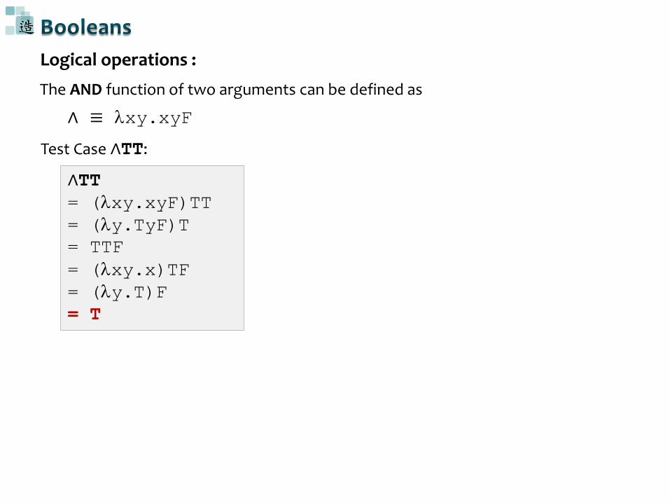
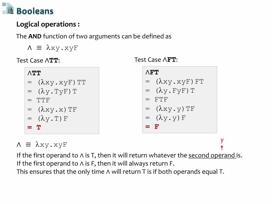
Logical operations :
The AND function of two arguments can be defined as
∧ ≡ xy.xyF
∧TT= (xy.xyF)TT
= (y.TyF)T
= TTF
= (xy.x)TF
= (y.T)F
= T
Test Case ∧TT:
Logical operations :
The AND function of two arguments can be defined as
∧ ≡ xy.xyF
∧TT= (xy.xyF)TT
= (y.TyF)T
= TTF
= (xy.x)TF
= (y.T)F
= T
Test Case ∧TT:
∧FT= (xy.xyF)FT
= (y.FyF)T
= FTF
= (xy.y)TF
= (y.y)F
= F
Test Case ∧FT:
If the first operand to ∧ is T, then it will return whatever the second operand is. If the first operand to ∧ is F, then it will always return F. This ensures that the only time ∧ will return T is if both operands equal T.
∧ ≡ xy.xyFy
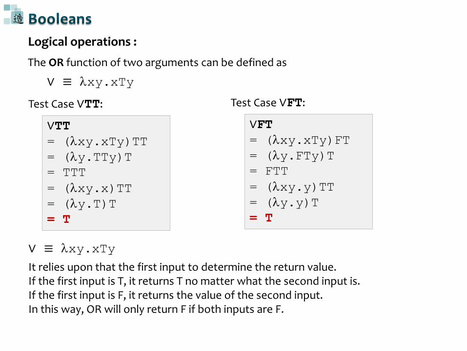
Logical operations :
The OR function of two arguments can be defined as
∨TT= (xy.xTy)TT
= (y.TTy)T
= TTT
= (xy.x)TT
= (y.T)T
= T
Test Case ∨TT:
∨FT= (xy.xTy)FT
= (y.FTy)T
= FTT
= (xy.y)TT
= (y.y)T
= T
Test Case ∨FT:
It relies upon that the first input to determine the return value. If the first input is T, it returns T no matter what the second input is. If the first input is F, it returns the value of the second input. In this way, OR will only return F if both inputs are F.
∨ ≡ xy.xTy
∨ ≡ xy.xTy
24
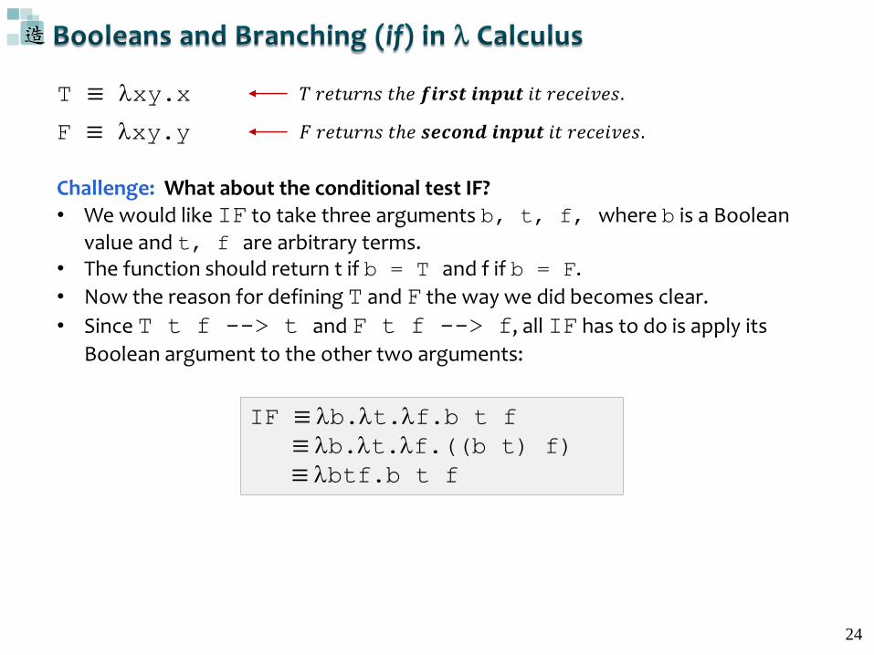
IF ≡ b.t.f.b t f
≡ b.t.f.((b t) f)≡ btf.b t f
T ≡ xy.x
F ≡ xy.y
𝑇 𝑟𝑒𝑡𝑢𝑟𝑛𝑠 𝑡ℎ𝑒 𝒇𝒊𝒓𝒔𝒕 𝒊𝒏𝒑𝒖𝒕 𝑖𝑡 𝑟𝑒𝑐𝑒𝑖𝑣𝑒𝑠.
𝐹 𝑟𝑒𝑡𝑢𝑟𝑛𝑠 𝑡ℎ𝑒 𝒔𝒆𝒄𝒐𝒏𝒅 𝒊𝒏𝒑𝒖𝒕 𝑖𝑡 𝑟𝑒𝑐𝑒𝑖𝑣𝑒𝑠.
Challenge: What about the conditional test IF? • We would like IF to take three arguments b, t, f, where b is a Boolean
value and t, f are arbitrary terms. • The function should return t if b = T and f if b = F.
• Now the reason for defining T and F the way we did becomes clear.
• Since T t f --> t and F t f --> f, all IF has to do is apply its
Boolean argument to the other two arguments:
6.25
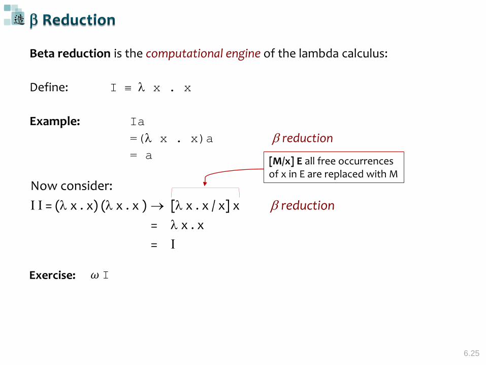
Beta reduction is the computational engine of the lambda calculus:
Define: I x . x
Example: Ia
=( x . x)a reduction
= a
Now consider:
I I = ( x . x) ( x . x ) [ x . x / x] x reduction
= x . x
= I
[M/x] E all free occurrences of x in E are replaced with M
Exercise: 𝜔 I
= x. (y. y+1) ((y. y+1) x)
= x. ((y. y+1) x) + 1
= x. (x+1) + 1
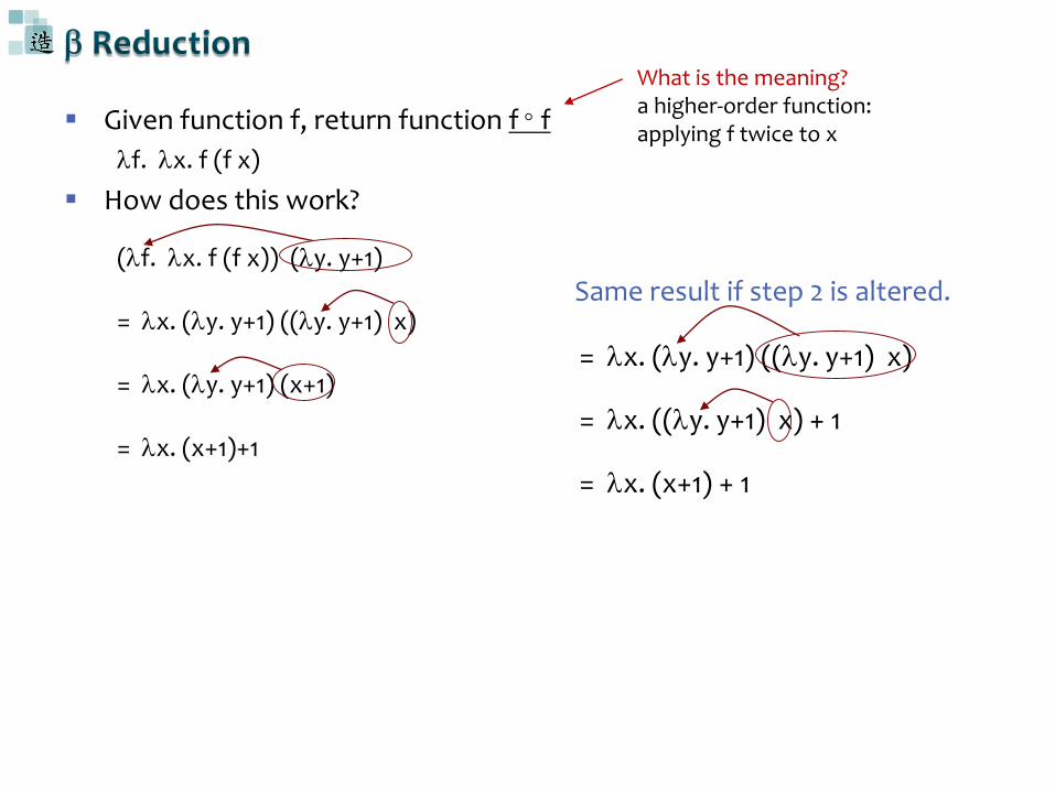
Given function f, return function f f
f. x. f (f x)
How does this work?
(f. x. f (f x)) (y. y+1)
= x. (y. y+1) ((y. y+1) x)
= x. (y. y+1) (x+1)
= x. (x+1)+1
Same result if step 2 is altered.
What is the meaning?a higher-order function:applying f twice to x
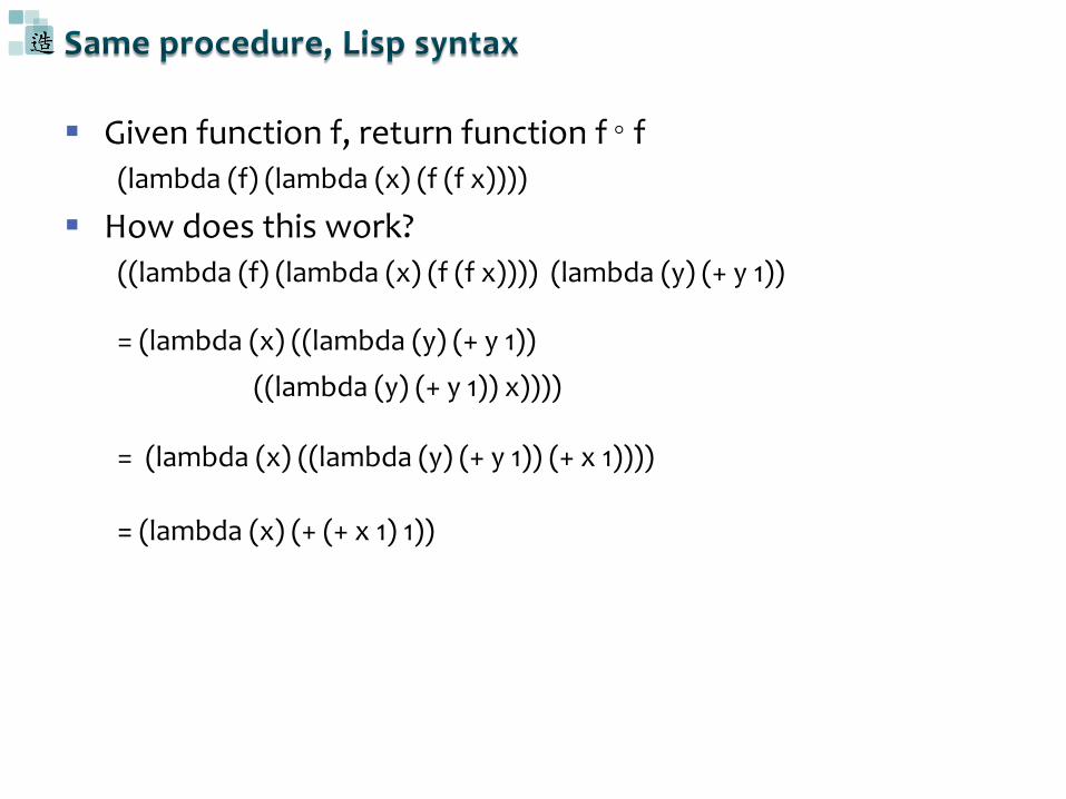
Given function f, return function f f(lambda (f) (lambda (x) (f (f x))))
How does this work?((lambda (f) (lambda (x) (f (f x)))) (lambda (y) (+ y 1))
= (lambda (x) ((lambda (y) (+ y 1))
((lambda (y) (+ y 1)) x))))
= (lambda (x) ((lambda (y) (+ y 1)) (+ x 1))))
= (lambda (x) (+ (+ x 1) 1))
6.28
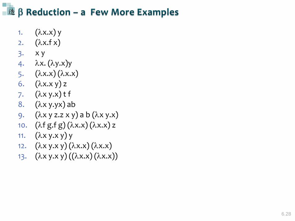
1. (x.x) y
2. (x.f x)
3. x y
4. x. (y.x)y
5. (x.x) (x.x)
6. (x.x y) z
7. (x y.x) t f
8. (x y.yx) ab
9. (x y z.z x y) a b (x y.x)
10. (f g.f g) (x.x) (x.x) z
11. (x y.x y) y
12. (x y.x y) (x.x) (x.x)
13. (x y.x y) ((x.x) (x.x))
6.29
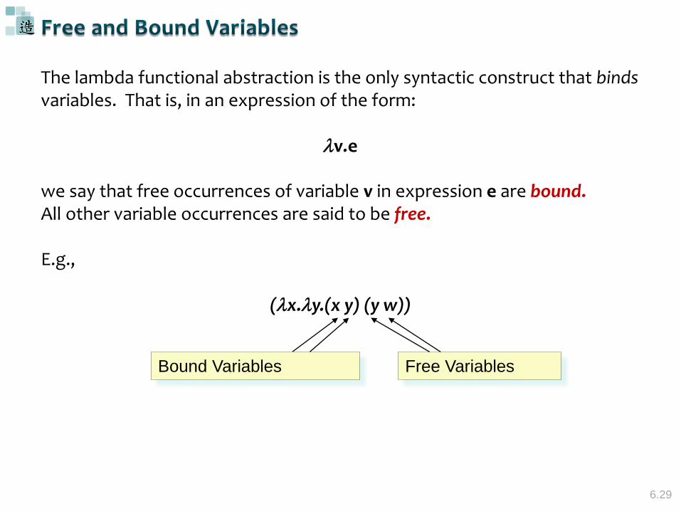
The lambda functional abstraction is the only syntactic construct that bindsvariables. That is, in an expression of the form:
v.e
we say that free occurrences of variable v in expression e are bound. All other variable occurrences are said to be free.
E.g.,
(x.y.(x y) (y w))
Free VariablesBound Variables
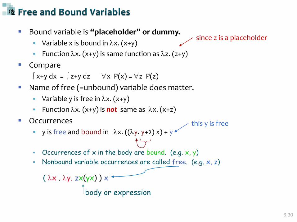
6.30
( x . y. zx(yx) ) x
body or expression
Bound variable is “placeholder” or dummy.
Variable x is bound in x. (x+y)
Function x. (x+y) is same function as z. (z+y)
Compare
x+y dx = z+y dz x P(x) = z P(z)
Name of free (=unbound) variable does matter.
Variable y is free in x. (x+y)
Function x. (x+y) is not same as x. (x+z)
Occurrences
y is free and bound in x. ((y. y+2) x) + y
Occurrences of x in the body are bound. (e.g. x, y)
Nonbound variable occurrences are called free. (e.g. x, z)
since z is a placeholder
this y is free
6.31
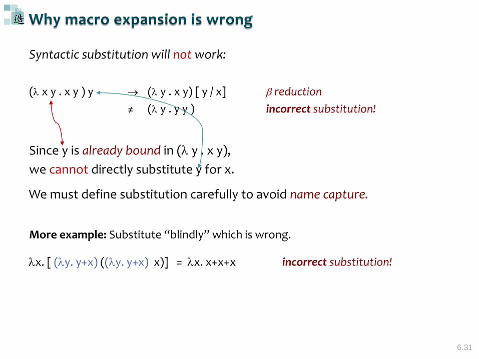
Syntactic substitution will not work:
( x y . x y ) y ( y . x y) [ y / x] reduction
≠ ( y . y y ) incorrect substitution!
Since y is already bound in ( y . x y),
we cannot directly substitute y for x.
We must define substitution carefully to avoid name capture.
x. [ (y. y+x) ((y. y+x) x)] = x. x+x+x
More example: Substitute “blindly” which is wrong.
incorrect substitution!
6.32
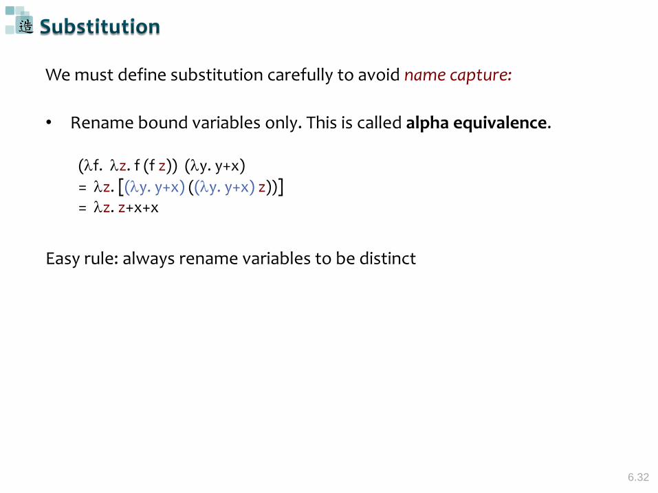
We must define substitution carefully to avoid name capture:
• Rename bound variables only. This is called alpha equivalence.
(f. z. f (f z)) (y. y+x)
= z. [(y. y+x) ((y. y+x) z))]= z. z+x+x
Easy rule: always rename variables to be distinct
33
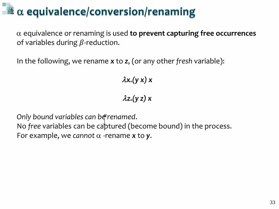
equivalence or renaming is used to prevent capturing free occurrences of variables during 𝛽-reduction.
In the following, we rename x to z, (or any other fresh variable):
x.(y x) x
z.(y z) x
Only bound variables can be renamed. No free variables can be captured (become bound) in the process. For example, we cannot -rename x to y.
α→
34
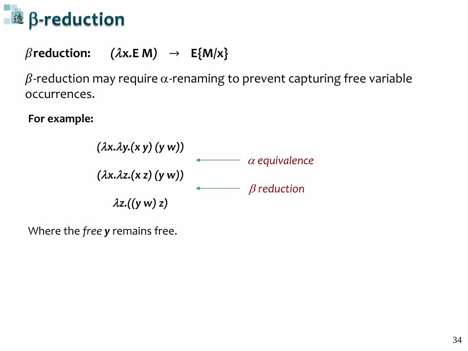
𝛽-reduction may require -renaming to prevent capturing free variable occurrences.
(x.E M) → E{M/x}𝛽reduction:
For example:
(x.y.(x y) (y w))
(x.z.(x z) (y w))
z.((y w) z)
Where the free y remains free.
equivalence
reduction
6.35
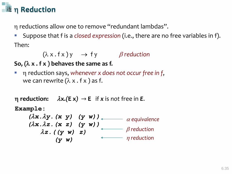
reductions allow one to remove “redundant lambdas”.
Suppose that f is a closed expression (i.e., there are no free variables in f).
Then:
( x . f x ) y f y reduction
So, ( x . f x ) behaves the same as f.
reduction says, whenever x does not occur free in f, we can rewrite ( x . f x ) as f.
Example:
(x.y.(x y) (y w))(x.z.(x z) (y w))
z.((y w) z)(y w)
equivalence
reduction
reduction
x.(E x) → E if x is not free in E. reduction:
6.36
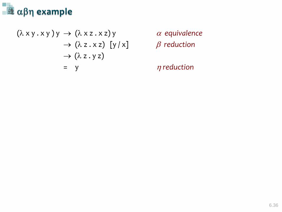
( x y . x y ) y ( x z . x z) y equivalence
( z . x z) [y / x] reduction
( z . y z)
= y reduction
6.37
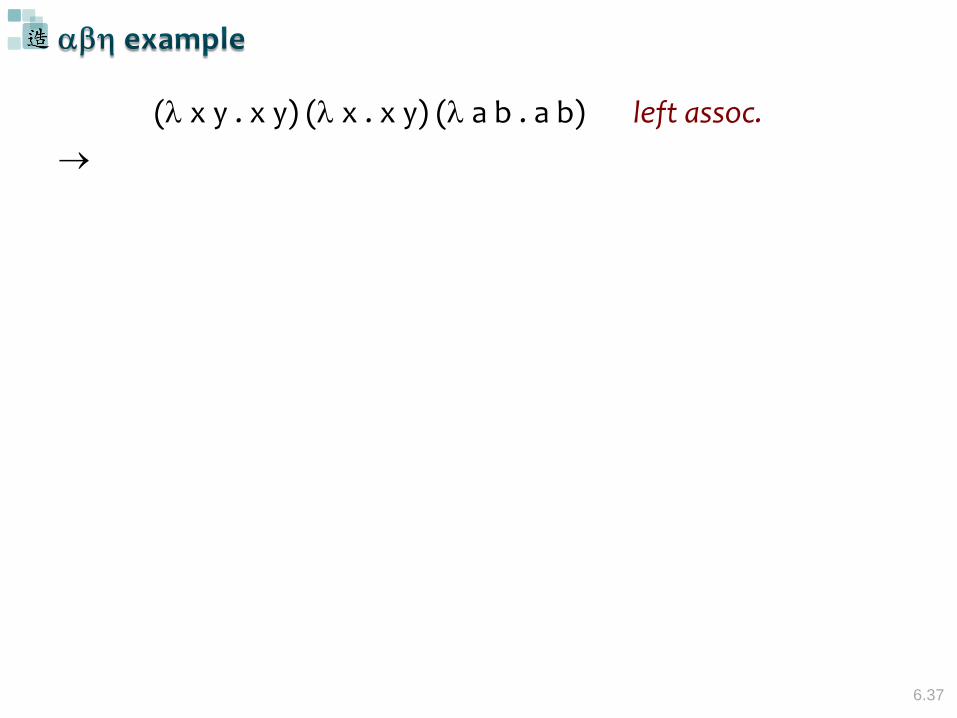
( x y . x y) ( x . x y) ( a b . a b) left assoc.
6.38
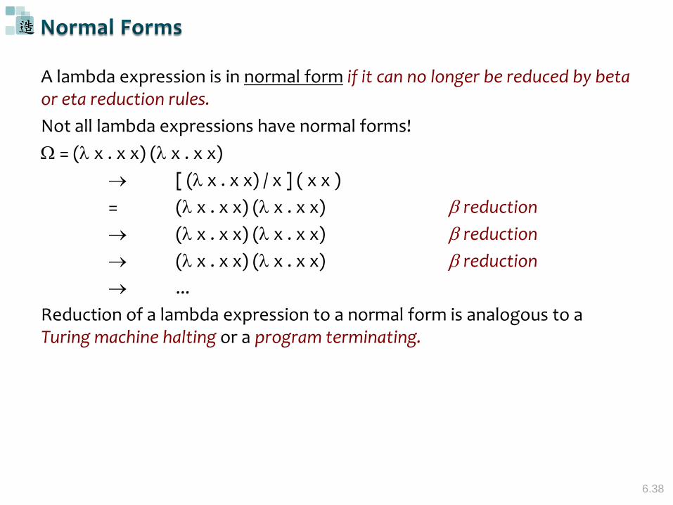
A lambda expression is in normal form if it can no longer be reduced by beta or eta reduction rules.
Not all lambda expressions have normal forms!
= ( x . x x) ( x . x x)
[ ( x . x x) / x ] ( x x )
= ( x . x x) ( x . x x) reduction
( x . x x) ( x . x x) reduction
( x . x x) ( x . x x) reduction
...
Reduction of a lambda expression to a normal form is analogous to a Turing machine halting or a program terminating.
6.39
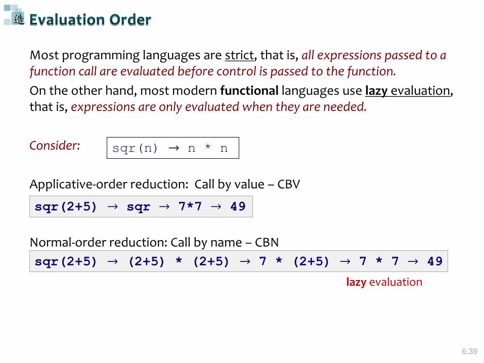
Most programming languages are strict, that is, all expressions passed to a function call are evaluated before control is passed to the function.
On the other hand, most modern functional languages use lazy evaluation, that is, expressions are only evaluated when they are needed.
Consider:
Applicative-order reduction: Call by value – CBV
Normal-order reduction: Call by name – CBN
sqr(n) → n * n
sqr(2+5) → sqr → 7*7 → 49
sqr(2+5) → (2+5) * (2+5) → 7 * (2+5) → 7 * 7 → 49
lazy evaluation
40
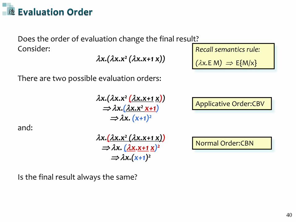
Does the order of evaluation change the final result?Consider:
x.(x.x2 (x.x+1 x))
There are two possible evaluation orders:
x.(x.x2 (x.x+1 x))x.(x.x2 x+1)x. (x+1)2
and:x.(x.x2 (x.x+1 x))x. (x.x+1 x)2
x.(x+1)2
Is the final result always the same?
Recall semantics rule:
(x.E M) E{M/x}
Applicative Order:CBV
Normal Order:CBN
41
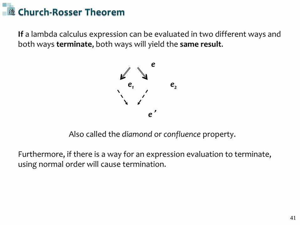
If a lambda calculus expression can be evaluated in two different ways and both ways terminate, both ways will yield the same result.
e
e1 e2
e’
Also called the diamond or confluence property.
Furthermore, if there is a way for an expression evaluation to terminate, using normal order will cause termination.

42
Consider:(x.y (x.(x x) x.(x x)))
There are two possible evaluation orders:
(x.y (x.(x x) x.(x x))) (x.y (x.(x x) x.(x x)))
and:(x.y (x.(x x) x.(x x)))
y
In this example, normal order terminates, whereas applicative order does not.
Recall semantics rule:
(x.E M) E{M/x}
Applicative Order:CBV
Normal Order:CBN

43
S: x.x2 (Square)I: x.x+1 (Increment)C: f.g.x.(f (g x)) (Function Composition)
((C S) I)
For example:
Function application:
Do you evaluate the output intuitively? (𝒙 + 𝟏)𝟐
How do you implement this function composition in Python?
44
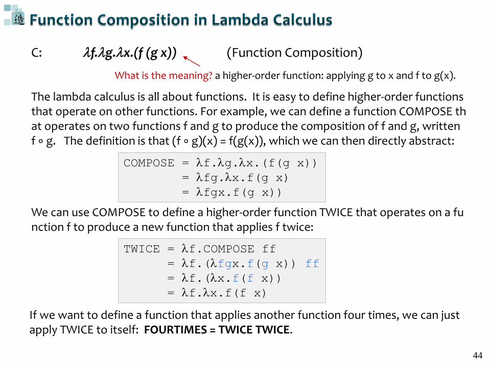
C: f.g.x.(f (g x)) (Function Composition)
What is the meaning? a higher-order function: applying g to x and f to g(x).
The lambda calculus is all about functions. It is easy to define higher-order functions that operate on other functions. For example, we can define a function COMPOSE that operates on two functions f and g to produce the composition of f and g, written f ∘ g. The definition is that (f ∘ g)(x) = f(g(x)), which we can then directly abstract:
COMPOSE = f.g.x.(f(g x))
= fg.x.f(g x)
= fgx.f(g x))
We can use COMPOSE to define a higher-order function TWICE that operates on a function f to produce a new function that applies f twice:
TWICE = f.COMPOSE ff
= f.(fgx.f(g x)) ff
= f.(x.f(f x))
= f.x.f(f x)
If we want to define a function that applies another function four times, we can just apply TWICE to itself: FOURTIMES = TWICE TWICE.
45
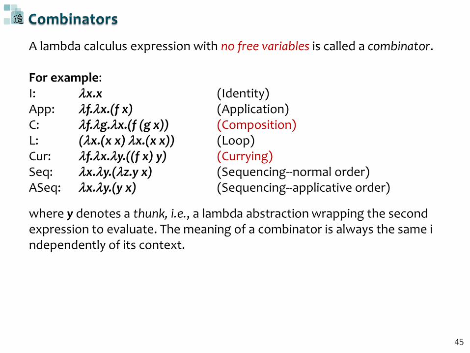
A lambda calculus expression with no free variables is called a combinator.
For example:I: x.x (Identity)App: f.x.(f x) (Application)C: f.g.x.(f (g x)) (Composition)L: (x.(x x) x.(x x)) (Loop)Cur: f.x.y.((f x) y) (Currying)Seq: x.y.(z.y x) (Sequencing--normal order)ASeq: x.y.(y x) (Sequencing--applicative order)
where y denotes a thunk, i.e., a lambda abstraction wrapping the second expression to evaluate. The meaning of a combinator is always the same independently of its context.
6.46
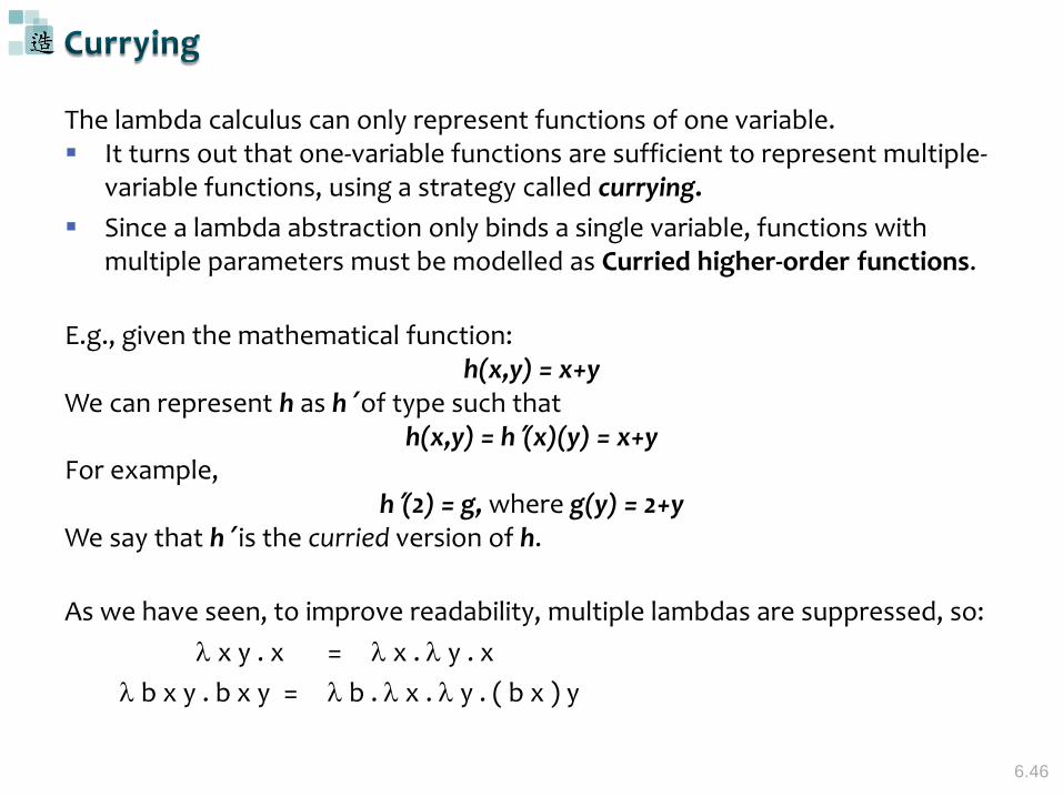
The lambda calculus can only represent functions of one variable. It turns out that one-variable functions are sufficient to represent multiple-
variable functions, using a strategy called currying.
Since a lambda abstraction only binds a single variable, functions with multiple parameters must be modelled as Curried higher-order functions.
E.g., given the mathematical function:h(x,y) = x+y
We can represent h as h’ of type such that h(x,y) = h’(x)(y) = x+y
For example, h’(2) = g, where g(y) = 2+y
We say that h’ is the curried version of h.
As we have seen, to improve readability, multiple lambdas are suppressed, so:
x y . x = x . y . x
b x y . b x y = b . x . y . ( b x ) y
47
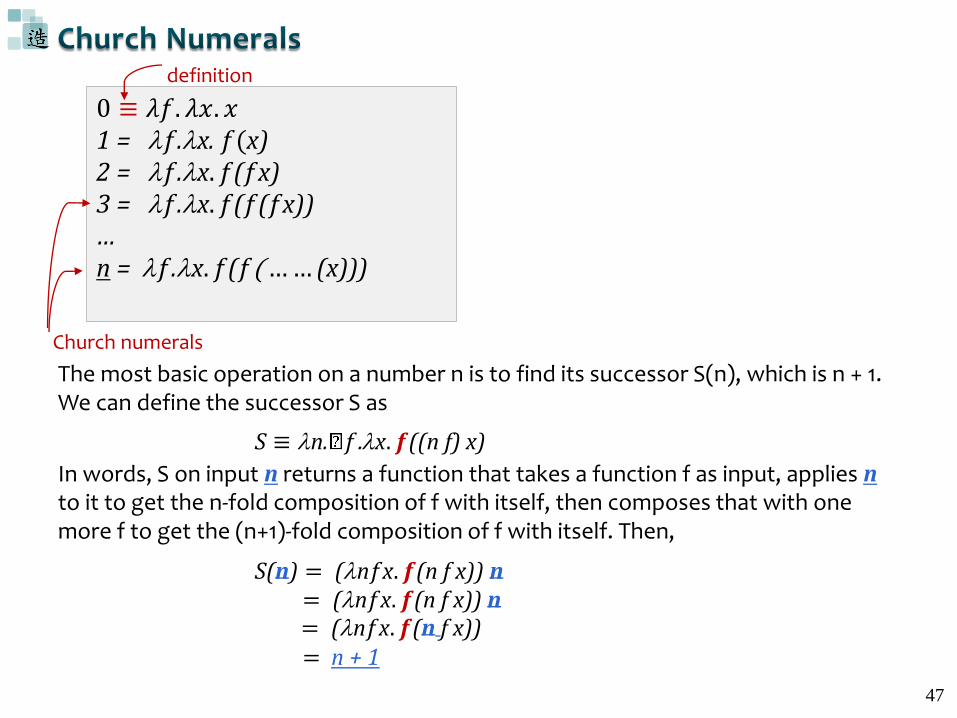
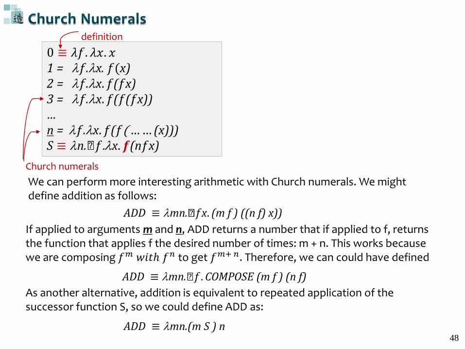
0 ≡ 𝜆𝑓. 𝜆𝑥. 𝑥1 = 𝑓.x. 𝑓(x)2 = 𝑓.x. 𝑓(𝑓x)3 = 𝑓.x. 𝑓(𝑓(𝑓x))…n = 𝑓.x. 𝑓(𝑓(…… (x)))
definition
Church numerals
The most basic operation on a number n is to find its successor S(n), which is n + 1. We can define the successor S as
S ≡ n. 𝑓.x. 𝒇((n f) x)
In words, S on input n returns a function that takes a function f as input, applies nto it to get the n-fold composition of f with itself, then composes that with one more f to get the (n+1)-fold composition of f with itself. Then,
S(n) = (n𝑓x. 𝒇(n f x)) n= (n𝑓x. 𝒇(n f x)) n= (n𝑓x. 𝒇(n f x))= n + 1
0 ≡ 𝜆𝑓. 𝜆𝑥. 𝑥1 = 𝑓.x. 𝑓(x)2 = 𝑓.x. 𝑓(𝑓x)3 = 𝑓.x. 𝑓(𝑓(𝑓x))…n = 𝑓.x. 𝑓(𝑓(…… (x)))S ≡ n. 𝑓.x. 𝒇(n𝑓x)
48
definition
Church numerals
We can perform more interesting arithmetic with Church numerals. We might define addition as follows:
ADD ≡ mn. 𝑓x. (m f ) ((n f) x))
If applied to arguments m and n, ADD returns a number that if applied to f, returns the function that applies f the desired number of times: m + n. This works because we are composing 𝑓𝑚 𝑤𝑖𝑡ℎ 𝑓𝑛 to get 𝑓𝑚+𝑛. Therefore, we can could have defined
ADD ≡ mn. 𝑓. COMPOSE (m f ) (n f)
As another alternative, addition is equivalent to repeated application of the successor function S, so we could define ADD as:
ADD ≡ mn.(m S ) n
49
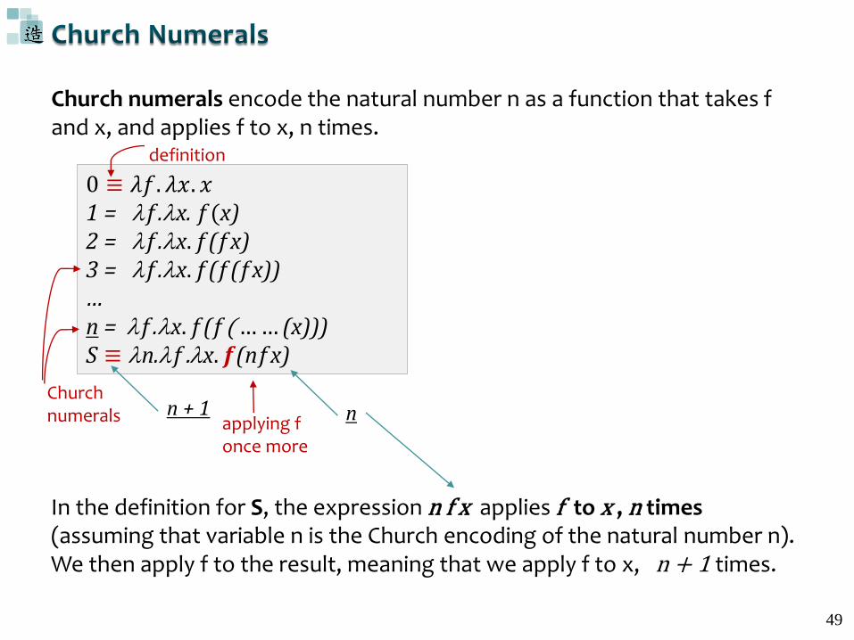
Church numerals encode the natural number n as a function that takes f and x, and applies f to x, n times.
0 ≡ 𝜆𝑓. 𝜆𝑥. 𝑥1 = 𝑓.x. 𝑓(x)2 = 𝑓.x. 𝑓(𝑓x)3 = 𝑓.x. 𝑓(𝑓(𝑓x))…n = 𝑓.x. 𝑓(𝑓(…… (x)))S ≡ n.𝑓.x. 𝒇(n𝑓x)
In the definition for S, the expression n f x applies f to x , n times (assuming that variable n is the Church encoding of the natural number n). We then apply f to the result, meaning that we apply f to x, n + 1 times.
applying fonce more
definition
Churchnumerals n + 1 n
50
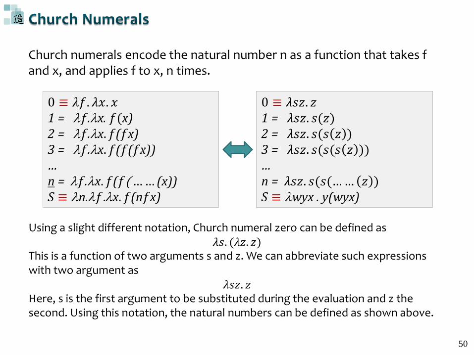
Church numerals encode the natural number n as a function that takes f and x, and applies f to x, n times.
0 ≡ 𝜆𝑓. 𝜆𝑥. 𝑥1 = 𝑓.x. 𝑓(x)2 = 𝑓.x. 𝑓(𝑓x)3 = 𝑓.x. 𝑓(𝑓(𝑓x))…n = 𝑓.x. 𝑓(𝑓(…… (x))S ≡ n.𝑓.x. 𝑓(n𝑓x)
Using a slight different notation, Church numeral zero can be defined as 𝜆𝑠. (𝜆𝑧. 𝑧)
This is a function of two arguments s and z. We can abbreviate such expressions with two argument as
𝜆𝑠𝑧. 𝑧Here, s is the first argument to be substituted during the evaluation and z the second. Using this notation, the natural numbers can be defined as shown above.
0 ≡ 𝜆𝑠𝑧. 𝑧1 = 𝜆𝑠𝑧. 𝑠(𝑧)2 = 𝜆𝑠𝑧. 𝑠(𝑠 𝑧 )3 = 𝜆𝑠𝑧. 𝑠(𝑠(𝑠 𝑧 ))…n = 𝜆𝑠𝑧. 𝑠(𝑠(…… 𝑧 )S ≡ wyx . y(wyx)
51
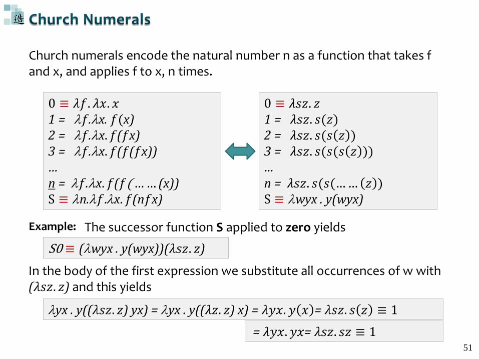
Church numerals encode the natural number n as a function that takes f and x, and applies f to x, n times.
S0 ≡ (wyx . y(wyx))(𝜆𝑠𝑧. 𝑧)
Example: The successor function S applied to zero yields
In the body of the first expression we substitute all occurrences of w with (𝜆𝑠𝑧. 𝑧) and this yields
yx . y((𝜆𝑠𝑧. 𝑧) yx) = yx . y((𝜆𝑧. 𝑧) x) = 𝜆𝑦𝑥. 𝑦 𝑥 = 𝜆𝑠𝑧. 𝑠 𝑧 ≡ 1
= 𝜆𝑦𝑥. 𝑦𝑥= 𝜆𝑠𝑧. 𝑠𝑧 ≡ 1
0 ≡ 𝜆𝑓. 𝜆𝑥. 𝑥1 = 𝑓.x. 𝑓(x)2 = 𝑓.x. 𝑓(𝑓x)3 = 𝑓.x. 𝑓(𝑓(𝑓x))…n = 𝑓.x. 𝑓(𝑓(…… (x))S ≡ n.𝑓.x. 𝑓(n𝑓x)
0 ≡ 𝜆𝑠𝑧. 𝑧1 = 𝜆𝑠𝑧. 𝑠(𝑧)2 = 𝜆𝑠𝑧. 𝑠(𝑠 𝑧 )3 = 𝜆𝑠𝑧. 𝑠(𝑠(𝑠 𝑧 ))…n = 𝜆𝑠𝑧. 𝑠(𝑠(…… 𝑧 )S ≡ wyx . y(wyx)
52
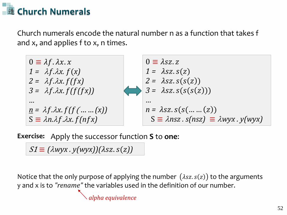
Church numerals encode the natural number n as a function that takes f and x, and applies f to x, n times.
S1 ≡ (wyx . y(wyx))(𝜆𝑠𝑧. 𝑠(𝑧))
Exercise: Apply the successor function S to one:
Notice that the only purpose of applying the number 𝜆𝑠𝑧. 𝑠 𝑧 to the arguments y and x is to "rename" the variables used in the definition of our number.
alpha equivalence
0 ≡ 𝜆𝑠𝑧. 𝑧1 = 𝜆𝑠𝑧. 𝑠(𝑧)2 = 𝜆𝑠𝑧. 𝑠(𝑠 𝑧 )3 = 𝜆𝑠𝑧. 𝑠(𝑠(𝑠 𝑧 ))…n = 𝜆𝑠𝑧. 𝑠(𝑠(…… 𝑧 )S ≡ nsz . s(nsz) ≡ wyx . y(wyx)
0 ≡ 𝜆𝑓. 𝜆𝑥. 𝑥1 = 𝑓.x. 𝑓(x)2 = 𝑓.x. 𝑓(𝑓x)3 = 𝑓.x. 𝑓(𝑓(𝑓x))…n = 𝑓.x. 𝑓(𝑓(…… (x))S ≡ n.𝑓.x. 𝑓(n𝑓x)
53
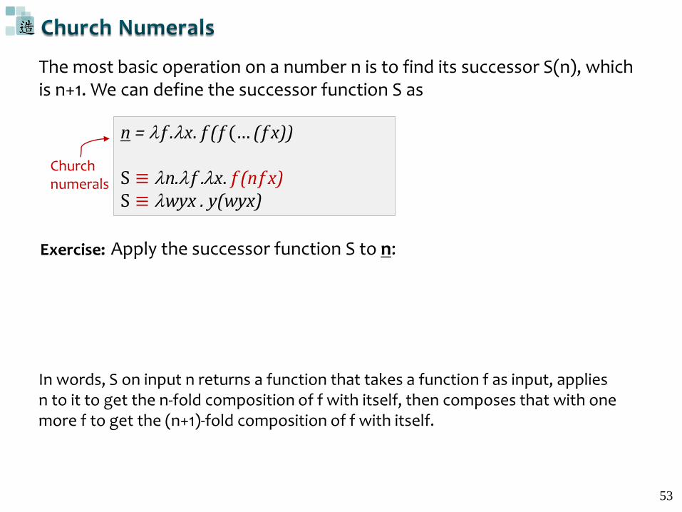
The most basic operation on a number n is to find its successor S(n), which is n+1. We can define the successor function S as
n = 𝑓.x. 𝑓(𝑓(… (𝑓x))
S ≡ n.𝑓.x. 𝑓(n𝑓x)S ≡ wyx . y(wyx)
Exercise: Apply the successor function S to n:
Churchnumerals
In words, S on input n returns a function that takes a function f as input, applies n to it to get the n-fold composition of f with itself, then composes that with one more f to get the (n+1)-fold composition of f with itself.
54
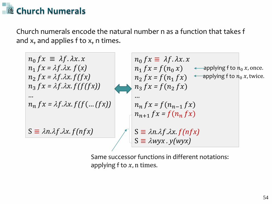
Church numerals encode the natural number n as a function that takes f and x, and applies f to x, n times.
𝑛0 𝑓𝑥 ≡ 𝜆𝑓. 𝜆𝑥. 𝑥𝑛1 𝑓𝑥 = 𝑓.x. 𝑓(x)𝑛2 𝑓𝑥 = 𝑓.x. 𝑓(𝑓x)𝑛3 𝑓𝑥 = 𝑓.x. 𝑓(𝑓(𝑓x))…𝑛𝑛 𝑓𝑥 = 𝑓.x. 𝑓(𝑓(… (𝑓x))
S ≡ n.𝑓.x. 𝑓(n𝑓x)
𝑛0 𝑓𝑥 ≡ 𝜆𝑓. 𝜆𝑥. 𝑥𝑛1 𝑓𝑥 = 𝑓(𝑛0 𝑥)𝑛2 𝑓𝑥 = 𝑓(𝑛1 𝑓𝑥)𝑛3 𝑓𝑥 = 𝑓(𝑛2 𝑓𝑥)…𝑛𝑛 𝑓𝑥 = 𝑓(𝑛𝑛−1 𝑓𝑥)𝑛𝑛+1 𝑓𝑥 = 𝑓(𝑛𝑛 𝑓𝑥)
S ≡ n.𝑓.x. 𝑓(n𝑓x)S ≡ wyx . y(wyx)
applying f to 𝑛0 𝑥, once.
applying f to 𝑛0 𝑥, twice.
Same successor functions in different notations: applying f to 𝑥, n times.
55
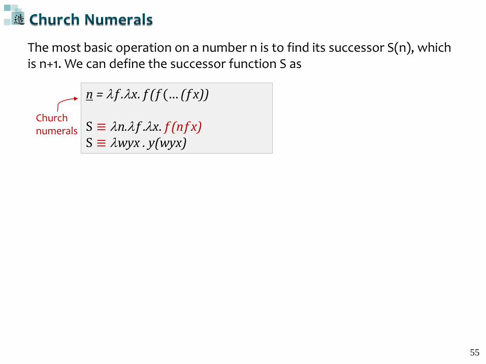
The most basic operation on a number n is to find its successor S(n), which is n+1. We can define the successor function S as
n = 𝑓.x. 𝑓(𝑓(… (𝑓x))
S ≡ n.𝑓.x. 𝑓(n𝑓x)S ≡ wyx . y(wyx)
Churchnumerals
56
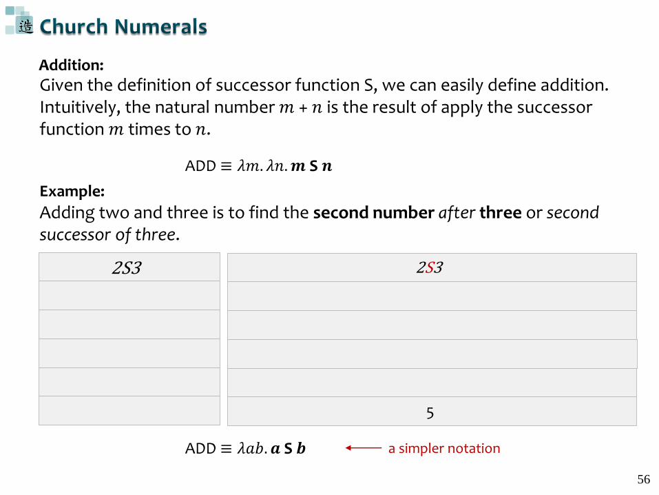
Given the definition of successor function S, we can easily define addition. Intuitively, the natural number 𝑚 + 𝑛 is the result of apply the successor function 𝑚 times to 𝑛.
ADD ≡ 𝜆𝑚. 𝜆𝑛.𝒎 S 𝒏
Addition:
Example:
Adding two and three is to find the second number after three or second successor of three.
2S3 2S3
5
ADD ≡ 𝜆𝑎𝑏. 𝒂 S 𝒃 a simpler notation
57
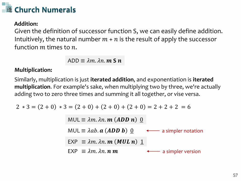
Given the definition of successor function S, we can easily define addition. Intuitively, the natural number 𝑚 + 𝑛 is the result of apply the successor function 𝑚 times to 𝑛.
ADD ≡ 𝜆𝑚. 𝜆𝑛.𝒎 S 𝒏
Addition:
Similarly, multiplication is just iterated addition, and exponentiation is iterated multiplication. For example's sake, when multiplying two by three, we're actually adding two to zero three times and summing it all together, or vise versa.
MUL ≡ 𝜆𝑚. 𝜆𝑛.𝒎 𝑨𝑫𝑫 𝒏 0
Multiplication:
2 ∗ 3 = 2 + 0 ∗ 3 = 2 + 0 + 2 + 0 + 2 + 0 = 2 + 2 + 2 = 6
MUL ≡ 𝜆𝑎𝑏. 𝒂 𝑨𝑫𝑫 𝒃 0 a simpler notation
EXP ≡ 𝜆𝑚. 𝜆𝑛.𝒎 𝑴𝑼𝑳 𝒏 1
EXP ≡ 𝜆𝑚. 𝜆𝑛. 𝒏 𝒎 a simpler version
58
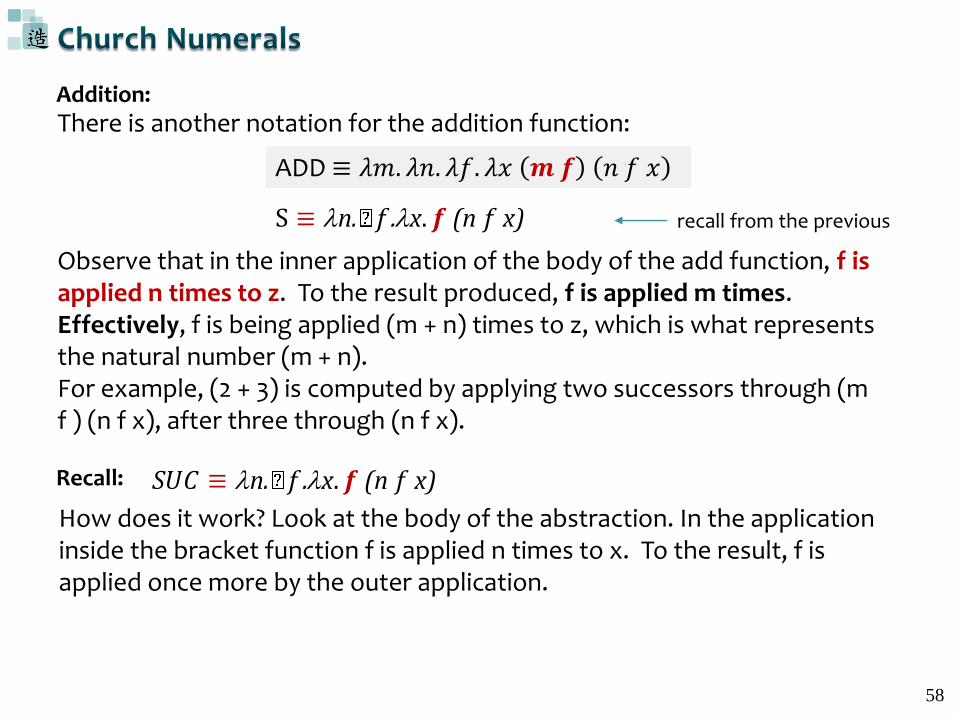
There is another notation for the addition function:
ADD ≡ 𝜆𝑚. 𝜆𝑛. 𝜆𝑓. 𝜆𝑥 𝒎 𝒇 𝑛 𝑓 𝑥
Addition:
S ≡ n. 𝑓.x. 𝒇 (n 𝑓 x)
Observe that in the inner application of the body of the add function, f is applied n times to z. To the result produced, f is applied m times. Effectively, f is being applied (m + n) times to z, which is what represents the natural number (m + n). For example, (2 + 3) is computed by applying two successors through (m f ) (n f x), after three through (n f x).
recall from the previous
Recall: S𝑈𝐶 ≡ n. 𝑓.x. 𝒇 (n 𝑓 x)
How does it work? Look at the body of the abstraction. In the application inside the bracket function f is applied n times to x. To the result, f is applied once more by the outer application.
59
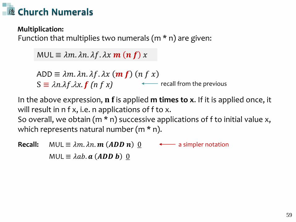
Function that multiplies two numerals (m * n) are given:
MUL ≡ 𝜆𝑚. 𝜆𝑛. 𝜆𝑓. 𝜆𝑥 𝒎 𝒏 𝒇 𝑥
Multiplication:
ADD ≡ 𝜆𝑚. 𝜆𝑛. 𝜆𝑓. 𝜆𝑥 𝒎 𝒇 𝑛 𝑓 𝑥
S ≡ n.𝜆𝑓.x. 𝒇 (n 𝑓 x) recall from the previous
In the above expression, n f is applied m times to x. If it is applied once, it will result in n f x, i.e. n applications of f to x. So overall, we obtain (m * n) successive applications of f to initial value x, which represents natural number (m * n).
MUL ≡ 𝜆𝑚. 𝜆𝑛.𝒎 𝑨𝑫𝑫 𝒏 0Recall: a simpler notation
MUL ≡ 𝜆𝑎𝑏. 𝒂 𝑨𝑫𝑫 𝒃 0
60
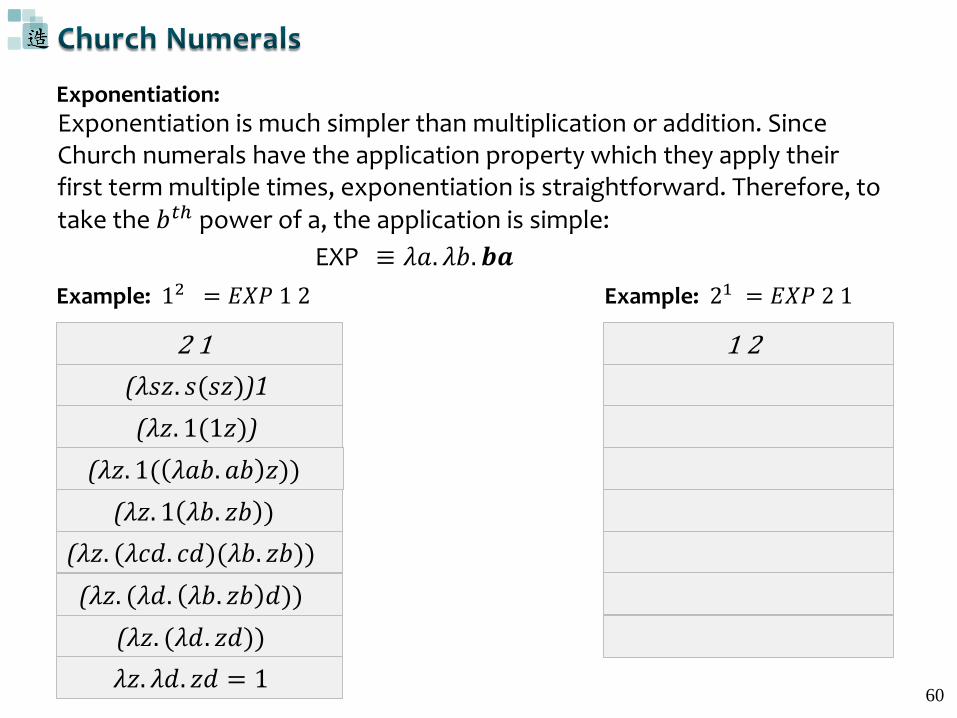
Exponentiation is much simpler than multiplication or addition. Since Church numerals have the application property which they apply their first term multiple times, exponentiation is straightforward. Therefore, to take the 𝑏𝑡ℎ power of a, the application is simple:
Exponentiation:
EXP ≡ 𝜆𝑎. 𝜆𝑏. 𝒃𝒂
Example: 12 = 𝐸𝑋𝑃 1 2
2 1
(𝜆𝑠𝑧. 𝑠(𝑠𝑧))1
(𝜆𝑧. 1(1𝑧))
(𝜆𝑧. 1( 𝜆𝑎𝑏. 𝑎𝑏 𝑧))
(𝜆𝑧. 1 𝜆𝑏. 𝑧𝑏 )
(𝜆𝑧. (𝜆𝑐𝑑. 𝑐𝑑)(𝜆𝑏. 𝑧𝑏))
(𝜆𝑧. (𝜆𝑑. 𝜆𝑏. 𝑧𝑏 𝑑))
(𝜆𝑧. (𝜆𝑑. 𝑧𝑑))
𝜆𝑧. 𝜆𝑑. 𝑧𝑑 = 1
Example: 21 = 𝐸𝑋𝑃 2 1
1 2
61
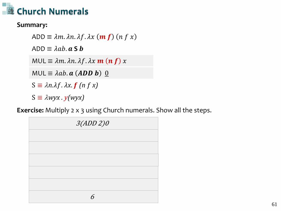
Exercise: Multiply 2 x 3 using Church numerals. Show all the steps.
MUL ≡ 𝜆𝑚. 𝜆𝑛. 𝜆𝑓. 𝜆𝑥 𝒎 𝒏 𝒇 𝑥
ADD ≡ 𝜆𝑚. 𝜆𝑛. 𝜆𝑓. 𝜆𝑥 𝒎 𝒇 𝑛 𝑓 𝑥
S ≡ n.𝜆𝑓. 𝜆x. 𝒇 (n 𝑓 x)
MUL ≡ 𝜆𝑎𝑏. 𝒂 𝑨𝑫𝑫 𝒃 0
S ≡ wyx . y(wyx)
ADD ≡ 𝜆𝑎𝑏. 𝒂 S 𝒃
Summary:
3(ADD 2)0
6
Summary
The lambda calculus is Turing complete.
The lambda calculus is the model of computation underlying functional programming languages.
References
http://www.cs.rice.edu/~javaplt/311/Readings/supplemental.pdf
http://www.utdallas.edu/~gupta/courses/apl/lambda.pdf
http://www.cse.iitb.ac.in/~rkj/lambda.pdf