‘safehull-dynamic loading approach’ for vessels · the safehull-dynamic loading approach...
TRANSCRIPT
G u i d e f o r ‘ S a f e H u l l - D y n a m i c L o a d i n g A p p r o a c h ’ f o r V e s s e l s
GUIDE FOR
‘SAFEHULL-DYNAMIC LOADING APPROACH’ FOR VESSELS
DECEMBER 2006 (Updated May 2018 – see next page)
American Bureau of Shipping Incorporated by Act of Legislature of the State of New York 1862
2010-2018 American Bureau of Shipping. All rights reserved. ABS Plaza 16855 Northchase Drive Houston, TX 77060 USA
Updates
May 2018 consolidation includes: • February 2017 version plus Notice No. 3
February 2017 consolidation includes: • January 2017 version plus Corrigenda/Editorials
January 2017 consolidation includes: • October 2015 version plus Corrigenda/Editorials
October 2015 consolidation includes: • February 2014 version plus Notice No. 2
February 2014 consolidation includes: • August 2013 version plus Corrigenda/Editorials
August 2013 consolidation includes: • December 2006 version plus Notice No. 1 and Corrigenda/Editorials
F o r e w o r d
Foreword This Guide provides information about the optional classification notation, SafeHull-Dynamic Loading Approach, SH-DLA, which is available to qualifying vessels intended to carry oil in bulk, ore or bulk cargoes, containers and liquefied gases in bulk. In the text herein, this document is referred to as “this Guide”.
Section 1-1-3 of the ABS Rules for Conditions of Classification (Part 1) contains descriptions of the various basic and optional classification notations available. The following Chapters of the ABS Rules for Building and Classing Steel Vessels (Steel Vessel Rules) give the design and analysis criteria applicable to the specific vessel types:
• Part 5C, Chapter 1 – Tankers of 150 meters (492 feet) or more in length
• Part 5C, Chapter 3 – Bulk carriers of 150 meters (492 feet) or more in length
• Part 5C, Chapter 5 – Container carriers of 130 meters (427 feet) or more in length
• Part 5C, Chapter 8 – LNG carriers
• Part 5C, Chapter 12 – Membrane Tank LNG Vessels
In addition to the Rule design criteria, SafeHull-Dynamic Loading Approach based on first-principle direct calculations is acceptable with respect to the determination of design loads and the establishment of strength criteria for vessels. In the case of a conflict between this Guide and the ABS Steel Vessel Rules, the latter has precedence.
This Guide is a consolidated and extended edition of:
• Analysis Procedure Manual for The Dynamic Loading Approach (DLA) for Tankers, March 1992
• Analysis Procedure Manual for The Dynamic Loading Approach (DLA) for Bulk Carriers, April 1993
• Analysis Procedure Manual for The Dynamic Loading Approach (DLA) for Container Carriers, April 1993
• Guidance Notes on ‘SafeHull-Dynamic Loading Approach’ for Container Carriers, April 2005
This Guide represents the most current and advanced ABS DLA analysis procedure including linear and nonlinear seakeeping analysis. This Guide is issued December 2006. Users of this Guide are welcome to contact ABS with any questions or comments concerning this Guide. Users are advised to check periodically with ABS to ensure that this version of this Guide is current.
ABS GUIDE FOR ‘SAFEHULL-DYNAMIC LOADING APPROACH’ FOR VESSELS . 2006 iii
T a b l e o f C o n t e n t s
GUIDE FOR
‘SAFEHULL-DYNAMIC LOADING APPROACH’ FOR VESSELS
CONTENTS SECTION 1 General .................................................................................................... 1
1 Introduction ......................................................................................... 1 3 Application ........................................................................................... 1 5 Concepts and Benefits of DLA Analysis ............................................. 1
5.1 Concepts ......................................................................................... 1 5.3 Benefits ............................................................................................ 2 5.5 Load Case Development for DLA Analysis ...................................... 2 5.7 General Modeling Considerations.................................................... 3
7 Notations ............................................................................................. 3 9 Scope and Overview of this Guide ..................................................... 3 FIGURE 1 Schematic Representation of the DLA Analysis Procedure ..... 5
SECTION 2 Load Cases ............................................................................................. 6
1 General ............................................................................................... 6 3 Ship Speed.......................................................................................... 6 5 Loading Conditions ............................................................................. 6
5.1 Tankers ............................................................................................ 6 5.3 Bulk Carriers .................................................................................... 7 5.5 Container Carriers ........................................................................... 7 5.7 LNG Carriers ................................................................................... 7
7 Dominant Load Parameters (DLP) ..................................................... 7 7.1 Tankers ............................................................................................ 7 7.3 Bulk Carriers .................................................................................... 9 7.5 Container Carriers ........................................................................... 9 7.7 LNG Carriers ................................................................................. 11
9 Instantaneous Load Components ..................................................... 11 11 Impact and Other Loads ................................................................... 12 13 Selection of Load Cases ................................................................... 12 FIGURE 1 Positive Vertical Bending Moment ............................................ 7 FIGURE 2 Positive Vertical Shear Force .................................................... 8 FIGURE 3 Definition of Ship Motions ......................................................... 8 FIGURE 4 Positive Horizontal Bending Moment ...................................... 10 FIGURE 5 Reference Point for Acceleration ............................................ 10
iv ABS GUIDE FOR ‘SAFEHULL-DYNAMIC LOADING APPROACH’ FOR VESSELS . 2006
SECTION 3 Environmental Condition ..................................................................... 13 1 General ............................................................................................. 13 3 Wave Scatter Diagram ...................................................................... 13 5 Wave Spectrum ................................................................................ 13 TABLE 1 IACS Wave Scatter Diagrams for the North Atlantic ............... 14 FIGURE 1 Definition of Wave Heading .................................................... 14
SECTION 4 Response Amplitude Operators ......................................................... 15
1 General ............................................................................................. 15 3 Static Loads ...................................................................................... 15 5 Linear Seakeeping Analysis.............................................................. 16
5.1 General Modeling Considerations ................................................. 16 5.3 Diffraction-Radiation Methods ....................................................... 16 5.5 Panel Model Development ............................................................ 16 5.7 Roll Damping Model ...................................................................... 16
7 Ship Motion and Wave Load RAOs .................................................. 16 SECTION 5 Long-term Response ........................................................................... 17
1 General ............................................................................................. 17 3 Short-term Response ........................................................................ 17 5 Long-Term Response ....................................................................... 18
SECTION 6 Equivalent Design Wave ...................................................................... 19
1 General ............................................................................................. 19 3 Equivalent Wave Amplitude .............................................................. 19 5 Wave Frequency and Heading ......................................................... 19 7 Linear Instantaneous Load Components .......................................... 20 9 Nonlinear Pressure Adjustment near the Waterline ......................... 20 11 Special Consideration to Adjust EWA for Maximum Hogging and
Sagging Load Cases ......................................................................... 21 FIGURE 1 Determination of Wave Amplitude .......................................... 20 FIGURE 2 Pressure Adjustment Zones .................................................... 21
SECTION 7 Nonlinear Ship Motion and Wave Load .............................................. 22
1 General ............................................................................................. 22 3 Nonlinear Seakeeping Analysis ........................................................ 22
3.1 Concept ......................................................................................... 22 3.3 Benefits of Nonlinear Seakeeping Analysis ................................... 22
5 Modeling Consideration .................................................................... 22 5.1 Mathematical Model ...................................................................... 22 5.3 Numerical Course-keeping Model ................................................. 23
7 Nonlinear Instantaneous Load Components .................................... 23
ABS GUIDE FOR ‘SAFEHULL-DYNAMIC LOADING APPROACH’ FOR VESSELS . 2006 v
SECTION 8 External Pressure ................................................................................. 24 1 General ............................................................................................. 24 3 Simultaneously-acting External Pressures ....................................... 24 5 Pressure Loading on the Structural FE Model .................................. 24 FIGURE 1 Sample External Hydrodynamic Pressure for Maximum
Hogging Moment Amidships ................................................... 24 SECTION 9 Internal Liquid Tank Pressure ............................................................. 25
1 General ............................................................................................. 25 3 Pressure Components ...................................................................... 25 5 Local Acceleration at the CG of Tank Content ................................. 26 7 Simultaneously-acting Tank Pressure .............................................. 26 FIGURE 1 Internal Pressure on a Completely Filled Tank ....................... 26 FIGURE 2 Internal Pressure on a Partially Filled Tank ............................ 26
SECTION 10 Bulk Cargo Pressure ............................................................................ 27
1 General ............................................................................................. 27 3 Definitions ......................................................................................... 27 5 Pressure Components ...................................................................... 28
5.1 Static Pressure .............................................................................. 28 5.3 Dynamic Pressure ......................................................................... 28
7 Local Acceleration at the CG of Tank Content ................................. 31 9 Simultaneously-acting Bulk Cargo Load ........................................... 31 FIGURE 1 Definition of Wall Angle α ........................................................ 27 FIGURE 2 Definition of Positive Tangential Component of Bulk Cargo
Pressure .................................................................................. 27 FIGURE 3 Static Pressure due to Gravity ................................................ 28 FIGURE 4 Dynamic Pressure due to Vertical Acceleration ...................... 29 FIGURE 5 Dynamic Pressure due to Transverse Acceleration ................ 30
SECTION 11 Container Load ..................................................................................... 32
1 General ............................................................................................. 32 3 Load Components ............................................................................. 32
3.1 Static Load ..................................................................................... 32 3.3 Dynamic Load ................................................................................ 32
5 Local Acceleration at the CG of a Container .................................... 33 7 Simultaneously-acting Container Load ............................................. 34 FIGURE 1 Dynamic Load due to Vertical and Transverse
Acceleration ............................................................................ 33
vi ABS GUIDE FOR ‘SAFEHULL-DYNAMIC LOADING APPROACH’ FOR VESSELS . 2006
SECTION 12 Load on Lightship Structure and Equipment .................................... 35 1 General ............................................................................................. 35 3 Load Components ............................................................................. 35
3.1 Static Load .................................................................................... 35 3.3 Dynamic Load ............................................................................... 35
5 Local Acceleration ............................................................................. 36 7 Simultaneously-acting Loads on Lightship Structure and
Equipment ......................................................................................... 36 SECTION 13 Loading for Structural FE Analysis .................................................... 37
1 General ............................................................................................. 37 3 Equilibrium Check ............................................................................. 37 5 Boundary Forces and Moments ........................................................ 37
SECTION 14 Structural FE Analysis ......................................................................... 38
1 General ............................................................................................. 38 3 Global FE Analysis ............................................................................ 38 5 Local FE Analysis ............................................................................. 38
5.1 Tanker ........................................................................................... 38 5.3 Bulk Carrier ................................................................................... 39 5.5 Container Carrier ........................................................................... 39 5.7 LNG Carrier ................................................................................... 39
7 Fatigue Assessment ......................................................................... 39 SECTION 15 Acceptance Criteria.............................................................................. 40
1 General ............................................................................................. 40 3 Yielding ............................................................................................. 40
3.1 Field Stress ................................................................................... 40 3.3 Local Stress ................................................................................... 41 3.5 Hot-Spot Stress ............................................................................. 41 3.7 Allowable Stress for Watertight Boundaries .................................. 41 3.9 Allowable Stresses for Main Supporting Members and
Structural Details ........................................................................... 41 5 Buckling and Ultimate Strength ........................................................ 42 TABLE 1 Allowable Stresses for Watertight Boundaries ........................ 41 TABLE 2 Allowable Stresses for Various FE Mesh Sizes
(Non-tight Structural Members) ............................................... 42 APPENDIX 1 Summary of Analysis Procedure ........................................................ 43
1 General ............................................................................................. 43 3 Basic Data Required ......................................................................... 43 5 Hydrostatic Calculations ................................................................... 43 7 Response Amplitude Operators (RAOs) ........................................... 44 9 Long-Term Extreme Values .............................................................. 44 11 Equivalent Design Waves ................................................................. 44
ABS GUIDE FOR ‘SAFEHULL-DYNAMIC LOADING APPROACH’ FOR VESSELS . 2006 vii
13 Nonlinear Seakeeping Analysis ........................................................ 45 15 External Pressure ............................................................................. 45 17 Internal Liquid Tank Pressure ........................................................... 45 19 Bulk Cargo Pressure ......................................................................... 45 21 Container Loads ................................................................................ 45 23 Loads on Lightship Structure and Equipment ................................... 45 25 Loadings for Structural FE Analysis .................................................. 46 27 Global FE Analysis ............................................................................ 46 29 Local FE Analysis ............................................................................. 46 31 Closing Comments ............................................................................ 47
APPENDIX 2 Buckling and Ultimate Strength Criteria ............................................. 48
1 General ............................................................................................. 48 1.1 Approach ....................................................................................... 48 1.3 Buckling Control Concepts ............................................................ 48
3 Plate Panels ...................................................................................... 48 3.1 Buckling State Limit ....................................................................... 48 3.3 Effective Width ............................................................................... 49 3.5 Ultimate Strength ........................................................................... 49
5 Longitudinals and Stiffeners .............................................................. 50 5.1 Beam-Column Buckling State Limits and Ultimate Strength .......... 50 5.3 Torsional-Flexural Buckling State Limit .......................................... 51
7 Stiffened Panels ................................................................................ 51 7.1 Large Stiffened Panels Between Bulkheads .................................. 51 7.3 Uniaxially Stiffened Panels between Transverses and Girders ..... 51
9 Deep Girders and Webs ................................................................... 52 9.1 Buckling Criteria............................................................................. 52 9.3 Tripping .......................................................................................... 52
APPENDIX 3 Nominal Design Corrosion Values (NDCV) for Vessels .................... 53
1 General ............................................................................................. 53 TABLE 1 Nominal Design Corrosion Values for Tankers ....................... 54 TABLE 2 Nominal Design Corrosion Values for Bulk Carriers ............... 56 TABLE 3 Nominal Design Corrosion Values for Container Carriers ...... 58 TABLE 4 Nominal Design Corrosion Values for Membrane LNG
Carriers ................................................................................... 60 FIGURE 1 Nominal Design Corrosion Values for Tankers ....................... 53 FIGURE 2 Nominal Design Corrosion Values for Bulk Carriers ............... 55 FIGURE 3 Nominal Design Corrosion Values for Container Carriers ...... 57 FIGURE 4 Nominal Design Corrosion Values for Membrane LNG
Carriers ................................................................................... 59
viii ABS GUIDE FOR ‘SAFEHULL-DYNAMIC LOADING APPROACH’ FOR VESSELS . 2006
S e c t i o n 1 : G e n e r a l
S E C T I O N 1 General
1 Introduction The design and construction of the hull, superstructure and deckhouses of an ocean-going vessel are to be based on all applicable requirements of the ABS Rules for Building and Classing Steel Vessels (Steel Vessel Rules). The design criteria of the Steel Vessel Rules are referred to as ABS SafeHull criteria.
The SafeHull criteria in the Steel Vessel Rules entail a two-step procedure. The main objective of the first step, referred to as Initial Scantling Evaluation (ISE), is scantling selection to accommodate global and local strength requirements. The scantling selection is accomplished through the application of design equations that reflect combinations of static and dynamic envelope loads; durability considerations; expected service, survey and maintenance practices; and structural strength considering the failure modes of material yielding and buckling. Also, a part of ISE is an assessment of fatigue strength primarily aimed at connections between longitudinal stiffeners and transverse web frames in the hull structure. The second step of the SafeHull criteria, referred to as Total Strength Assessment (TSA), entails the performance of structural analyses using the primary design Loading Cases of ISE. The main purpose of the TSA analyses is to confirm that the selected design scantlings are adequate (from a broader structural system point of view) to resist the failure modes of yielding, buckling, ultimate strength and fatigue.
The SafeHull-Dynamic Loading Approach (SH-DLA) provides an enhanced structural analyses basis to assess the capabilities and sufficiency of a structural design. A fundamental requirement of SH-DLA is that the basic, initial design of the structure is to be in accordance with the SafeHull criteria as specified in the Steel Vessel Rules. The results of the DLA analyses cannot be used to reduce the basic scantlings obtained from the direct application of the Rule criteria scantling requirements (see 3-1-2/5.3 of the Steel Vessel Rules). However, should the DLA analysis indicate the need to increase any basic scantling, this increase is to be accomplished to meet the DLA criteria.
3 Application (1 May 2018) This Guide is applicable to ocean-going vessels of all size and proportions including tankers, bulk carriers, container carriers and LNG carriers. Specifically for a container carrier with length in excess of 290 meters (951 feet), the hull structure and critical structural details are to comply with the requirements of this SafeHull-Dynamic Loading Approach (5C-5-1/1.3.3 of the Steel Vessel Rules).
5 Concepts and Benefits of DLA Analysis
5.1 Concepts DLA is an analysis process, rather than a step-wise design-oriented process such as SafeHull criteria. The DLA Analysis emphasizes the completeness and realism of the analysis model in terms of both the extent of the structure modeled and the loading conditions analyzed. The DLA modeling and analysis process relies on performing multiple levels of analysis that start with an overall or global hull model. The results of each previous level of analysis are used to establish which areas of the structure require finer (more detailed) modeling and analysis, as well as the local loads and ‘boundary conditions’ to be imposed on the finer model.
The Load Cases considered in the DLA Analysis possess the following attributes: i) Use of cargo loading patterns, other loading components and vessel operating drafts that reflect
the actual ones intended for the vessel (note that the Load Cases in SafeHull comprise mainly those intended to produce ‘scantling design controlling’ situations).
ii) Load components that are realistically combined to assemble each DLA Analysis Load Case. The dynamically related aspects of the components are incorporated in the model, and the combination of these dynamically considered components is accommodated in the analysis method.
ABS GUIDE FOR ‘SAFEHULL-DYNAMIC LOADING APPROACH’ FOR VESSELS . 2006 1
Section 1 General
5.3 Benefits The enhanced realism provided by the DLA analysis gives benefits that are of added value to the Owner/Operator. The most important of these is an enhanced and more precise quantification of structural safety based on the attributes mentioned above. Additionally, the more specific knowledge of expected structural behavior and performance is very useful in more realistically evaluating and developing inspection and maintenance plans. The usefulness of such analytical results when discussing the need to provide possible future steel renewals should be apparent. A potentially valuable benefit that can arise from the DLA analysis is that it provides access to a comprehensive and authoritative structural evaluation model, which may be readily employed in the event of emergency situations that might occur during the service life, such as structural damage, repairs or modifications.
5.5 Load Case Development for DLA Analysis The basic concept, which must be understood to grasp the nature of DLA, concerns the creation of each Load Case to be used in the DLA analysis. A Load Case contains a Dominant Load component that is characterized by a Dominant Load Parameter (DLP) and the instantaneous load components accompanying the Dominant Load component.
A load component consists of dynamic and static parts. For example, the load component “external fluid pressure on the vessel’s hull in the presence of waves” has a hydrostatic component that combines with a dynamic pressure component. The determination of the static part of the load component is basic. The dynamic part reflects the wave-induced motion effects, which are the product of an inertial portion of the load and a portion representing the motion-induced displacement of the load relative to the structure’s axis system.
Examples of Dominant Load Parameters are “Vertical Bending Moment Amidships” and “Vertical Acceleration at Bow”. The specific Dominant Load Parameters that are recommended for inclusion in the DLA Analysis of each vessel type are given in Subsection 2/7. The other instantaneous load components accompanying the Dominant Load component in a Load Case include internal and external fluid pressures and lightship weights, including structural self-weight.
The combination of the load components composing a Load Case is done through a process where each Dominant Load is analyzed to establish its Response Amplitude Operator (RAO). Using a combination of ship motion analysis, involving ocean wave spectra, and extreme value analysis of the Dominant Load Parameter, an equivalent design wave is derived. The design wave (defined by wave amplitude, frequency, heading and phase angle with respect to a selected reference location) is considered equivalent in the sense that when it is imposed on the structural model it simulates the extreme value of the DLP. The process to perform this derivation is given in Sections 4, 5 and 6.
In this Guide, emphasis is given to the development of hydrodynamic loadings based on seakeeping analysis. It is assumed that the user has the needed theoretical background and computational tools for seakeeping and spectral analysis, which are required in the determination of the Load Cases.
From the seakeeping analysis, the instantaneous magnitude and spatial distributions of the Dominant Load component and the other load components accompanying the Dominant Load component are to be obtained. The procedures to establish these load components accompanying the DLP are given for the various other load component types in Sections 6, 7, 8, 9 and 10.
Using the described basic procedure there are many additional considerations and refinements that can be included and accommodated in DLA Analysis. These include items such as the following:
i) Operational considerations of the vessel in extreme waves
ii) Directionality of waves
iii) Energy spreading of sea spectra
iv) Various formulations to characterize the sea spectra
v) Various exceedance probability levels to characterize extreme values of Dominant Load Parameters
2 ABS GUIDE FOR ‘SAFEHULL-DYNAMIC LOADING APPROACH’ FOR VESSELS . 2006
Section 1 General
The point to bear in mind is that the procedure is robust enough to accommodate these items. In addition it is to be noted that the DLA analysis could also be carried out considering Load Cases comprised of Dominant Stress values and Dominant Stress Parameter, in lieu of Dominant Load components and Dominant Load Parameter, in much the same manner as previously described. In such case the combination of the stress components, rather than load components, comprising a Load Case, can be done through a process where each Dominant Stress is analyzed to establish its stress RAO. This generally requires much more extensive calculations to determine the stress values in the many dynamic conditions and therefore is beyond the scope of this Guide.
5.7 General Modeling Considerations In general, it is expected that the inaccuracies and uncertainties, which can arise from use of partial or segmented models, will be minimized by the use of models that are sufficiently comprehensive and complete to meet the goals of the analysis. This specifically means that to the maximum extent practicable, the overall model of the vessel should comprise the entire hull structure. The motion analysis should consider the effect of all six degrees of freedom motions. There is also to be sufficient compatibility between the hydrodynamic and structural models so that the application of hydrodynamic pressures onto the finite element mesh of the structural model can be done appropriately.
The results of overall (global) FE analysis are to be directly employed in the analysis of the required finer mesh, local FE models. Appropriate ‘boundary conditions’ determined in the larger scale model are to be imposed on the local models to assure appropriate structural continuity and load transfer between the various levels of models.
7 Notations The SH-DLA notation signifies the satisfaction of the DLA analysis procedure of this Guide. The notation SH-DLA signifies:
i) The design is based on an analysis which more explicitly considers the loads acting on the structure and their dynamic nature, and
ii) In no case is an offered design scantling to be less than that obtained from other requirements in the Steel Vessel Rules.
In this regard, all the supporting data, analysis procedures and calculated results are to be fully documented and submitted for review.
9 Scope and Overview of this Guide This Guide provides a description of the analysis procedures to be pursued to obtain the optional classification notation SafeHull-Dynamic Loading Approach, SH-DLA. Emphasis is given here to the determination of dynamic loads rather than the structural FEM analysis procedure. This has been done mainly because structural analysis practices are well established and understood among designers, but the dynamic load determination is a less familiar subject. Therefore, the procedures for FEM analysis are only briefly described for ready reference and completeness.
The Dynamic Loading Approach uses explicitly determined dynamic loads, and the results of the analysis are used as the basis to increase scantlings where indicated, but allows no decreases in scantlings from those obtained from the direct application of the Rules’ scantling equations.
While outside the scope of this Guide, the local impact pressure and global whipping loads due to slamming are to be separately addressed for the strength assessment of the hull structure. Also, the green sea loads due to the shipment of green water on deck is to be addressed for the scantlings of the forecastle deck and breakwater. For this purpose, the adequacy of the selected software may need to be demonstrated to the satisfaction of ABS.
ABS GUIDE FOR ‘SAFEHULL-DYNAMIC LOADING APPROACH’ FOR VESSELS . 2006 3

Section 1 General
This Guide systematically introduces the assumptions in the load formulations and the methods used in the response analysis underlying the DLA analysis. These include the following topics:
i) Specification of the loading conditions
ii) Specification of the Dominant Load Parameters
iii) Response Amplitude Operators and extreme values
iv) Equivalent design waves
v) Wave-induced load components and the assembly of Load Cases
vi) Structural FE model development
vii) Permissible stresses used in the acceptance criteria.
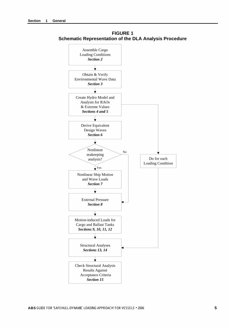
Refer to Section 1, Figure 1 for a schematic of the DLA analysis procedure.
While the DLA can, in principle, be applied to all forms of floating marine structures, the focus of this Guide is on tankers, bulk carriers, container carriers and LNG carriers. In the case of other ship types clients should consult with ABS to establish appropriate analysis parameters. This applies particularly to the choice of loading conditions and Dominant Load Parameters.
4 ABS GUIDE FOR ‘SAFEHULL-DYNAMIC LOADING APPROACH’ FOR VESSELS . 2006
Section 1 General
FIGURE 1 Schematic Representation of the DLA Analysis Procedure
Assemble CargoLoading Conditions
Section 2
Obtain & VerifyEnvironmental Wave Data
Section 3
Create Hydro Model andAnalysis for RAOs& Extreme ValuesSections 4 and 5
Do for eachLoading Condition
Derive EquivalentDesign Waves
Section 6
Nonlinear Ship Motionand Wave Loads
Section 7
Structural AnalysesSections 13, 14
Check Structural AnalysisResults Against
Acceptance CriteriaSection 15
External PressureSection 8
Motion-induced Loads forCargo and Ballast Tanks
Sections 9, 10, 11, 12
Nonlinearseakeepinganalysis?
Yes
No
ABS GUIDE FOR ‘SAFEHULL-DYNAMIC LOADING APPROACH’ FOR VESSELS . 2006 5
S e c t i o n 2 : L o a d C a s e s
S E C T I O N 2 Load Cases
1 General The Dynamic Loading Approach (DLA) requires the development of Load Cases to be investigated using the Finite Element (FE) structural analysis. The Load Cases are derived mainly based on the ship speed (see Subsection 2/3), loading conditions (see Subsection 2/5), and Dominant Load Parameters (see Subsection 2/7).
For each Load Case, the applied loads to be developed for structural FE analysis are to include both the static and dynamic parts of each load component. The dynamic loads represent the combined effects of a dominant load and other accompanying loads acting simultaneously on the hull structure, including external wave pressures, internal tank pressures, bulk cargo loads, container loads and inertial loads on the structural components and equipment. In quantifying the dynamic loads, it is necessary to consider a range of sea conditions and headings, which produce the considered critical responses of the hull structure.
For each Load Case, the developed loads are then used in the FE analysis to determine the resulting stresses and other load effects within the hull structure.
3 Ship Speed In general, the speed of a vessel in heavy weather may be significantly reduced in a voluntary and involuntary manner. In this Guide, for the strength assessment of tankers and bulk carriers, the ship speed is assumed to be zero in design wave conditions, which is consistent with IACS Rec. No.34. For the strength assessment of container and LNG carriers with finer hull forms, the ship speed is assumed to be five knots in design wave conditions.
5 Loading Conditions The loading conditions herein refer to the cargo and ballast conditions that are to be used for DLA analysis. The following loading conditions, typically found in the Loading Manual, are provided as a guideline to the most representative loading conditions to be considered in the DLA analysis.
Other cargo loading conditions that may be deemed critical can also be considered in the DLA analysis. The need to consider other loading conditions or additional loading conditions is to be determined in consultation with ABS.
5.1 Tankers i) Homogeneous full load condition at scantling draft
ii) Partial load condition (67% full)
iii) Partial load condition (50% full)
iv) Partial load condition (33% full)
v) Normal ballast load condition
6 ABS GUIDE FOR ‘SAFEHULL-DYNAMIC LOADING APPROACH’ FOR VESSELS . 2006
Section 2 Load Cases
5.3 Bulk Carriers i) Homogeneous full load condition at scantling draft
ii) Alternate full load condition at scantling draft
iii) Alternate load condition (67% full)
iv) Heavy ballast load condition
v) Light ballast load condition
5.5 Container Carriers i) Full load condition at scantling draft
ii) Light container full load condition with maximum SWBM amidships
iii) Partial load or jump load condition with highest GM
5.7 LNG Carriers i) Homogeneous full load condition at scantling draft
ii) Normal ballast load condition
iii) One tank empty condition
iv) Two adjacent tanks empty condition
7 Dominant Load Parameters (DLP) Dominant Load Parameters (DLP) refer to the load effects, arising from ship motions and wave loads, that may yield the maximum structural response for critical structural members. The instantaneous response of the vessel can be judged by one of the several Dominant Load Parameters. These parameters are to be maximized to establish Load Cases for the DLA analysis.
Other DLPs that may be deemed critical can also be considered in the DLA analysis. The need to consider other DLPs or additional DLPs is to be determined in consultation with ABS.
7.1 Tankers Below five Dominant Load Parameters have been identified as necessary to develop the Load Cases for tankers:
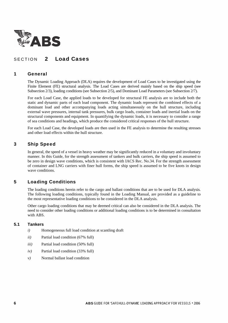
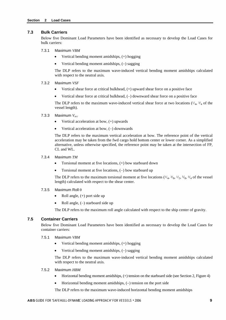
7.1.1 Maximum VBM • Vertical bending moment amidships, (+) hogging (see Section 2, Figure 1)
• Vertical bending moment amidships, (−) sagging
The DLP refers to the maximum wave-induced vertical bending moment amidships calculated with respect to the neutral axis.
FIGURE 1 Positive Vertical Bending Moment
(+)
ABS GUIDE FOR ‘SAFEHULL-DYNAMIC LOADING APPROACH’ FOR VESSELS . 2006 7
Section 2 Load Cases
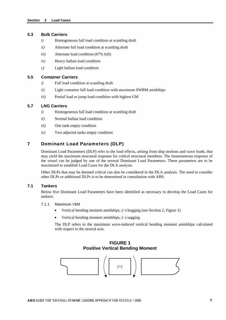
7.1.2 Maximum VSF • Vertical shear force, (+) upward shear force on a positive face (see Section 2, Figure 2)
• Vertical shear force, (–) downward shear force on a positive face
The DLP refers to the maximum wave-induced vertical shear force at two locations (1/4, 3/4 of the vessel length).
FIGURE 2 Positive Vertical Shear Force
(+)
7.1.3 Maximum Vacc • Vertical acceleration at FP, (+) upward
• Vertical acceleration at FP, (−) downward
The DLP refers to the maximum vertical acceleration at bow. The reference point of the vertical acceleration may be taken from the fwd tank top center or corner. As a simplified alternative, unless otherwise specified, the reference point may be taken at the intersection of FP, CL and WL.
7.1.4 Maximum Lacc
• Lateral acceleration at bow, (+) towards portside
• Lateral acceleration at bow, (−) towards starboard side
The DLP refers to the maximum lateral acceleration at bow. The lateral acceleration may be taken at the same reference point for vertical acceleration.
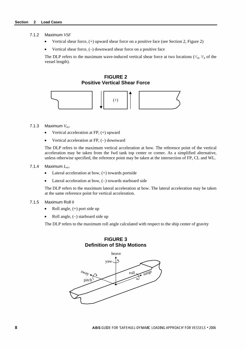
7.1.5 Maximum Roll θ • Roll angle, (+) port side up
• Roll angle, (−) starboard side up
The DLP refers to the maximum roll angle calculated with respect to the ship center of gravity
FIGURE 3 Definition of Ship Motions
heave
pitch
yaw
rollsway surge
8 ABS GUIDE FOR ‘SAFEHULL-DYNAMIC LOADING APPROACH’ FOR VESSELS . 2006
Section 2 Load Cases 7.3 Bulk Carriers
Below five Dominant Load Parameters have been identified as necessary to develop the Load Cases for bulk carriers:
7.3.1 Maximum VBM • Vertical bending moment amidships, (+) hogging
• Vertical bending moment amidships, (−) sagging
The DLP refers to the maximum wave-induced vertical bending moment amidships calculated with respect to the neutral axis.
7.3.2 Maximum VSF • Vertical shear force at critical bulkhead, (+) upward shear force on a positive face
• Vertical shear force at critical bulkhead, (−) downward shear force on a positive face
The DLP refers to the maximum wave-induced vertical shear force at two locations (1/4, 3/4 of the vessel length).
7.3.3 Maximum Vacc • Vertical acceleration at bow, (+) upwards
• Vertical acceleration at bow, (−) downwards
The DLP refers to the maximum vertical acceleration at bow. The reference point of the vertical acceleration may be taken from the fwd cargo hold bottom center or lower corner. As a simplified alternative, unless otherwise specified, the reference point may be taken at the intersection of FP, CL and WL.
7.3.4 Maximum TM • Torsional moment at five locations, (+) bow starboard down
• Torsional moment at five locations, (−) bow starboard up
The DLP refers to the maximum torsional moment at five locations (1/4, 3/8, 1/2, 5/8, 3/4 of the vessel length) calculated with respect to the shear center.
7.3.5 Maximum Roll θ • Roll angle, (+) port side up
• Roll angle, (−) starboard side up
The DLP refers to the maximum roll angle calculated with respect to the ship center of gravity.
7.5 Container Carriers Below five Dominant Load Parameters have been identified as necessary to develop the Load Cases for container carriers:
7.5.1 Maximum VBM • Vertical bending moment amidships, (+) hogging
• Vertical bending moment amidships, (−) sagging
The DLP refers to the maximum wave-induced vertical bending moment amidships calculated with respect to the neutral axis.
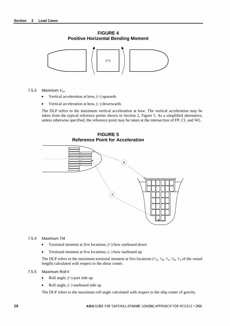
7.5.2 Maximum HBM • Horizontal bending moment amidships, (+) tension on the starboard side (see Section 2, Figure 4)
• Horizontal bending moment amidships, (−) tension on the port side
The DLP refers to the maximum wave-induced horizontal bending moment amidships
ABS GUIDE FOR ‘SAFEHULL-DYNAMIC LOADING APPROACH’ FOR VESSELS . 2006 9
Section 2 Load Cases
FIGURE 4 Positive Horizontal Bending Moment
(+)
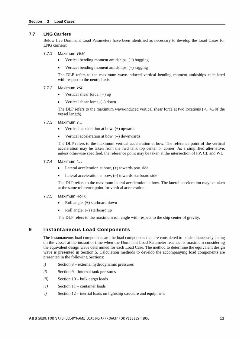
7.5.3 Maximum Vacc • Vertical acceleration at bow, (+) upwards
• Vertical acceleration at bow, (−) downwards
The DLP refers to the maximum vertical acceleration at bow. The vertical acceleration may be taken from the typical reference points shown in Section 2, Figure 5. As a simplified alternative, unless otherwise specified, the reference point may be taken at the intersection of FP, CL and WL.
FIGURE 5 Reference Point for Acceleration
A
B
7.5.4 Maximum TM • Torsional moment at five locations, (+) bow starboard down
• Torsional moment at five locations, (−) bow starboard up
The DLP refers to the maximum torsional moment at five locations (1/4, 3/8, 1/2, 5/8, 3/4 of the vessel length) calculated with respect to the shear center.
7.5.5 Maximum Roll θ • Roll angle, (+) port side up
• Roll angle, (−) starboard side up
The DLP refers to the maximum roll angle calculated with respect to the ship center of gravity.
10 ABS GUIDE FOR ‘SAFEHULL-DYNAMIC LOADING APPROACH’ FOR VESSELS . 2006
Section 2 Load Cases 7.7 LNG Carriers
Below five Dominant Load Parameters have been identified as necessary to develop the Load Cases for LNG carriers:
7.7.1 Maximum VBM • Vertical bending moment amidships, (+) hogging
• Vertical bending moment amidships, (−) sagging
The DLP refers to the maximum wave-induced vertical bending moment amidships calculated with respect to the neutral axis.
7.7.2 Maximum VSF • Vertical shear force, (+) up
• Vertical shear force, (−) down
The DLP refers to the maximum wave-induced vertical shear force at two locations (1/4, 3/4 of the vessel length).
7.7.3 Maximum Vacc • Vertical acceleration at bow, (+) upwards
• Vertical acceleration at bow, (−) downwards
The DLP refers to the maximum vertical acceleration at bow. The reference point of the vertical acceleration may be taken from the fwd tank top center or corner. As a simplified alternative, unless otherwise specified, the reference point may be taken at the intersection of FP, CL and WL
7.7.4 Maximum Lacc
• Lateral acceleration at bow, (+) towards port side
• Lateral acceleration at bow, (−) towards starboard side
The DLP refers to the maximum lateral acceleration at bow. The lateral acceleration may be taken at the same reference point for vertical acceleration.
7.7.5 Maximum Roll θ • Roll angle, (+) starboard down
• Roll angle, (−) starboard up
The DLP refers to the maximum roll angle with respect to the ship center of gravity.
9 Instantaneous Load Components The instantaneous load components are the load components that are considered to be simultaneously acting on the vessel at the instant of time when the Dominant Load Parameter reaches its maximum considering the equivalent design wave determined for each Load Case. The method to determine the equivalent design wave is presented in Section 5. Calculation methods to develop the accompanying load components are presented in the following Sections:
i) Section 8 – external hydrodynamic pressures
ii) Section 9 – internal tank pressures
iii) Section 10 – bulk cargo loads
iv) Section 11 – container loads
v) Section 12 – inertial loads on lightship structure and equipment
ABS GUIDE FOR ‘SAFEHULL-DYNAMIC LOADING APPROACH’ FOR VESSELS . 2006 11
Section 2 Load Cases 11 Impact and Other Loads
Impact loads due to bow flare and bottom slamming and other loads including green sea loads, tank fluid sloshing, vibrations, thermal loads and ice loads may affect global and local structural strength. These are not included in the DLA analysis, but the loads resulting from these considerations are to be treated separately in accordance with the current Steel Vessel Rules requirements.
13 Selection of Load Cases Load Cases are the cases to be investigated in the required structural FE analysis for DLA. Each Load Case is defined by a combination of ship speed (Subsection 2/3), loading condition (Subsection 2/5), a specified DLP (Subsection 2/7) and instantaneous loads accompanying the DLP (Subsection 2/9).
For the DLP of interest, the equivalent design wave is to be determined from the linear seakeeping analysis (Section 4) and long-term spectral analysis (Section 5). With the derived equivalent design wave (Section 6), the instantaneous loads accompanying the DLP are to be determined from linear seakeeeping analysis with nonlinear adjustment (Subsections 6/9 and 6/11) or directly from the nonlinear seakeeping analysis (Section 7).
A large number of Load Cases may result from the combination of loading conditions and the DLPs. Each Load Case is to be examined by performing the ship motion and wave load analysis. In general, not all the Load Cases may need to be included in the FE analysis. If necessary, the analyst may judiciously screen and select the critical Load Cases for the comprehensive structural FE analyses.
12 ABS GUIDE FOR ‘SAFEHULL-DYNAMIC LOADING APPROACH’ FOR VESSELS . 2006
ABS GUIDE FOR ‘SAFEHULL-DYNAMIC LOADING APPROACH’ FOR VESSELS . 2006 13
S e c t i o n 3 : E n v i r o n m e n t a l C o n d i t i o n
S E C T I O N 3 Environmental Condition
1 General For ocean-going vessels, environmentally-induced loads are dominated by waves, which are characterized by significant heights, spectral shapes and associated wave periods.
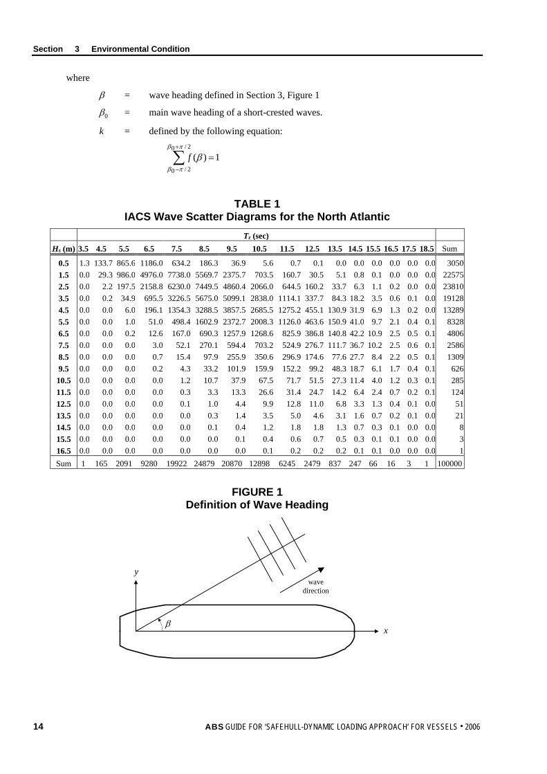
Unless otherwise specified, the vessel is assumed to operate for unrestricted service in the North Atlantic Ocean. IACS Recommendation No.34 (Nov. 2001) provides the standard wave data for the North Atlantic Ocean. It covers areas 8, 9, 15 and 16 of the North Atlantic defined in IACS Recommendation No. 34. The wave scatter diagram is used to calculate the extreme sea loads. In general, the long-term response at the level of 10-8 probability of exceedance ordinarily corresponds to a return period of about 25 years.
3 Wave Scatter Diagram The wave scatter diagram provides the probability or number of occurrences of sea states in a specified ocean area. Section 3, Table 1 shows the wave scatter diagram recommended by IACS for the North Atlantic. For a given zero-crossing period, Tz, and significant wave height, Hs, each cell represents the number of occurrence of the sea state out of 100,000 sea states.
5 Wave Spectrum The two-parameter Bretschneider spectrum is to be used to model the open sea wave conditions and the “cosine squared” spreading is to be applied to model the short-crest waves. The wave spectrum can be expressed by the following equation:
45
24
)/(25.1exp16
5)(
p
sp HS
where
S = wave energy density, in m2-sec
Hs = significant wave height, in meters
= angular frequency of wave component, in rad/sec
p = peak frequency, in rad/sec
= 2/Tp
Tp = peak period, in sec
= 1.408 Tz
The “cosine squared” spreading function is defined by:
f() = k cos2( – 0)
Section 3 Environmental Condition
where
β = wave heading defined in Section 3, Figure 1
β0 = main wave heading of a short-crested waves.
k = defined by the following equation:
∑+
−
=2/0
2/0
1)(πβ
πβ
βf
TABLE 1 IACS Wave Scatter Diagrams for the North Atlantic
Tz (sec) Hs (m) 3.5 4.5 5.5 6.5 7.5 8.5 9.5 10.5 11.5 12.5 13.5 14.5 15.5 16.5 17.5 18.5 Sum
0.5 1.3 133.7 865.6 1186.0 634.2 186.3 36.9 5.6 0.7 0.1 0.0 0.0 0.0 0.0 0.0 0.0 3050 1.5 0.0 29.3 986.0 4976.0 7738.0 5569.7 2375.7 703.5 160.7 30.5 5.1 0.8 0.1 0.0 0.0 0.0 22575 2.5 0.0 2.2 197.5 2158.8 6230.0 7449.5 4860.4 2066.0 644.5 160.2 33.7 6.3 1.1 0.2 0.0 0.0 23810 3.5 0.0 0.2 34.9 695.5 3226.5 5675.0 5099.1 2838.0 1114.1 337.7 84.3 18.2 3.5 0.6 0.1 0.0 19128 4.5 0.0 0.0 6.0 196.1 1354.3 3288.5 3857.5 2685.5 1275.2 455.1 130.9 31.9 6.9 1.3 0.2 0.0 13289 5.5 0.0 0.0 1.0 51.0 498.4 1602.9 2372.7 2008.3 1126.0 463.6 150.9 41.0 9.7 2.1 0.4 0.1 8328 6.5 0.0 0.0 0.2 12.6 167.0 690.3 1257.9 1268.6 825.9 386.8 140.8 42.2 10.9 2.5 0.5 0.1 4806 7.5 0.0 0.0 0.0 3.0 52.1 270.1 594.4 703.2 524.9 276.7 111.7 36.7 10.2 2.5 0.6 0.1 2586 8.5 0.0 0.0 0.0 0.7 15.4 97.9 255.9 350.6 296.9 174.6 77.6 27.7 8.4 2.2 0.5 0.1 1309 9.5 0.0 0.0 0.0 0.2 4.3 33.2 101.9 159.9 152.2 99.2 48.3 18.7 6.1 1.7 0.4 0.1 626
10.5 0.0 0.0 0.0 0.0 1.2 10.7 37.9 67.5 71.7 51.5 27.3 11.4 4.0 1.2 0.3 0.1 285 11.5 0.0 0.0 0.0 0.0 0.3 3.3 13.3 26.6 31.4 24.7 14.2 6.4 2.4 0.7 0.2 0.1 124 12.5 0.0 0.0 0.0 0.0 0.1 1.0 4.4 9.9 12.8 11.0 6.8 3.3 1.3 0.4 0.1 0.0 51 13.5 0.0 0.0 0.0 0.0 0.0 0.3 1.4 3.5 5.0 4.6 3.1 1.6 0.7 0.2 0.1 0.0 21 14.5 0.0 0.0 0.0 0.0 0.0 0.1 0.4 1.2 1.8 1.8 1.3 0.7 0.3 0.1 0.0 0.0 8 15.5 0.0 0.0 0.0 0.0 0.0 0.0 0.1 0.4 0.6 0.7 0.5 0.3 0.1 0.1 0.0 0.0 3 16.5 0.0 0.0 0.0 0.0 0.0 0.0 0.0 0.1 0.2 0.2 0.2 0.1 0.1 0.0 0.0 0.0 1 Sum 1 165 2091 9280 19922 24879 20870 12898 6245 2479 837 247 66 16 3 1 100000
FIGURE 1 Definition of Wave Heading
y
x
wavedirection
β
14 ABS GUIDE FOR ‘SAFEHULL-DYNAMIC LOADING APPROACH’ FOR VESSELS . 2006
S e c t i o n 4 : R e s p o n s e A m p l i t u d e O p e r a t o r s
S E C T I O N 4 Response Amplitude Operators
1 General This Section describes the Response Amplitude Operators (RAOs) of the ship motions and wave loads, which are the vessel’s responses to unit amplitude, regular, sinusoidal waves. Linear seakeeping analysis is to be performed to calculate the ship motions and wave loads for a number of wave headings and frequencies. These RAOs will be used to determine the long-term extreme values of Dominant Load Parameters. Also, these RAOs will be used to determine the equivalent design wave system.
Below, static load determination is described first, to be followed by the linear seakeeping analysis procedure to determine the dynamic ship motion and wave load RAOs.
3 Static Loads For each cargo loading condition, with a vessel’s hull geometry, lightship and deadweight as inputs, the hull girder shear force and bending moment distributions of the vessel in still water are to be computed at transverse sections along the vessel length. A sufficient number of lightship and dead weights are to be used to accurately represent the weight distribution of the vessel.
At a statically balanced loading condition, the displacement, trim and draft, Longitudinal Center of Buoyancy (LCB), transverse metacentric height (GMT) and longitudinal metacentric height (GML), should be checked to meet the following tolerances:
Displacement: ±1%
Trim: ±0.1 degrees
Draft:
Forward ±1 cm
Aft ±1 cm
LCB: ±0.1% of length
GMT: ±2%
GML: ±2%
SWBM: ±5%
Additionally, the longitudinal locations of the maximum and minimum still-water bending moments and, if appropriate, that of zero SWBM may be checked to assure proper distribution of the SWBM along the vessel’s length.
ABS GUIDE FOR ‘SAFEHULL-DYNAMIC LOADING APPROACH’ FOR VESSELS . 2006 15
Section 4 Response Amplitude Operators
5 Linear Seakeeping Analysis
5.1 General Modeling Considerations The same offset data and loading conditions used in the static load calculations are to be used for linear seakeeping analysis. Linear seakeeping analysis is to be performed for all loading conditions considered in Subsection 2/5. For each loading condition, the draft at F.P. and A.P., the location of center of gravity, radii of gyration and sectional mass distribution along the ship length are to be prepared from the Loading Manual. The free surface GM correction is to be considered for partially filled tanks. For full tank above 98% filling or empty tank below 2% filling, the free surface GM correction may be ignored.
There should be sufficient compatibility between the hydrodynamic and structural models so that the application of external hydrodynamic pressures onto the finite element mesh of the structural model can be done appropriately.
5.3 Diffraction-Radiation Methods Computations of the ship motion and wave load RAOs are to be carried out through the application of linear seakeeping analysis codes utilizing three-dimensional potential flow based diffraction-radiation theory. 3D panel methods or equivalent computer programs may be used to perform these calculations. All six degrees-of-freedom rigid-body motions of the vessel are to be accounted for.
5.5 Panel Model Development Boundary element methods, in general, require that the wetted surface of the vessel be discretized into a sufficiently large number of panels. The panel mesh should be fine enough to resolve the radiation and diffraction waves with reasonable accuracy.
5.7 Roll Damping Model The roll motion of a vessel in beam or oblique seas is greatly affected by viscous roll damping, especially with wave frequencies near the roll resonance. For seakeeping analysis based on potential flow theory, a proper viscous roll damping model is required. Experimental data or empirical methods can be used for the determination of the viscous roll damping. In addition to the hull viscous damping, the roll damping due to rudders and bilge keels is to be considered. If this information is not available, 10% of critical damping may be used for overall viscous roll damping.
7 Ship Motion and Wave Load RAOs The Response Amplitude Operators are first to be calculated for the Dominant Load Parameters for each of loading conditions specified in Subsection 2/5. Only these Dominant Load Parameters will be considered for the calculation of long-term extreme values.
A sufficient range of wave headings and frequencies should be considered for the calculation of the long-term extreme value of each Dominant Load Parameter. The Response Amplitude Operators are to be calculated for wave headings from head seas (180 deg.) to following seas (0 deg.) in increments of 15 deg. The range of wave frequencies is to include at least from 0.2 rad/s to 1.20 rad/s in increments of 0.05 rad/s.
If the ship motion and wave load analysis is performed in time domain, the analysis is to be performed for each regular wave with unit amplitude. In this case, the time histories of the ship motion and wave load responses are to be converted into RAOs by a suitable method (e.g., Fourier analysis). The time simulation is to be performed until the response reaches its steady state. The first half of time history is to be treated as transient period.
From the RAO of each DLP, the wave frequency-heading (ω, β) combination at which the RAO has its maximum will be used to determine the equivalent design waves of Section 5. In general, it is likely that the DLPs of VBM and VSF have their RAO maximum in the head sea condition, while the DLPs of HBM, TM, Vacc, Lacc, and Φ have their RAO maximum in beam or oblique sea conditions.
16 ABS GUIDE FOR ‘SAFEHULL-DYNAMIC LOADING APPROACH’ FOR VESSELS . 2006
ABS GUIDE FOR ‘SAFEHULL-DYNAMIC LOADING APPROACH’ FOR VESSELS . 2006 17
S e c t i o n 5 : L o n g - t e r m R e s p o n s e
S E C T I O N 5 Long-term Response
1 General The long-term response of each Dominant Load Parameter described in Subsection 2/7 is to be calculated for various loading conditions based on the wave scatter diagram (see Subsection 3/3) and the Response Amplitude Operators (see Subsection 4/7). The long-term response refers to the long-term most probable extreme value of the response at a specific probability level of exceedance. In general, the exceedance probability level of 10-8 corresponds to approximately 25 design years.
First, the short-term response of each Dominant Load Parameter is to be calculated for each sea state specified in wave scatter diagram. Combining the short-term responses and wave statistics consisting of the wave scatter diagram, the long-term response is to be calculated for each DLP under consideration.
3 Short-term Response For each sea state, a spectral density function Sy() of the response under consideration may be calculated , within the scope of linear theory, from the following equation:
Sy() = S ()|H()|2
where S() represents the wave spectrum and H() represents the Response Amplitude Operator (RAO, see Section 4) as a function of the wave frequency denoted by .. For a vessel with constant forward speed U, the n-th order spectral moment of the response may be expressed by the following equation:
0
2/0
2/0
)()(
dSfm yn
en
where f represents spreading function defined in Section 3 and e represents the wave frequency of encounter defined by:
cos2
gUe
where
g = gravitational acceleration
= wave heading angle (see Section 3, Figure 1)
Assuming the wave-induced response is a Gaussian stochastic process with zero mean and the spectral density function Sy() is narrow banded, the probability density function of the maxima (peak values) may be represented by a Rayleigh distribution. Then, the short-term probability of the response exceeding x0, Pr{x0} for the j-th sea state may be expressed by the following equation:
jjm
xx
0
20
02
exp}{Pr
As an alternative method, Ochi’s (1978) method may also be used considering the bandwidth of the wave spectra.
Section 5 Long-term Response
5 Long-Term Response The long-term probability of the response exceeding x0, Pr{x0} may be expressed by the following equation, expressed as a summation of joint probability over the short-term sea states:
∑∑=i
jj
ji xppx }{Pr}Pr{ 00
where
pi = probability of the i-th main wave heading angle
pj = probability of occurrence of the j-th sea state defined in wave scatter diagram
Prj{x0} = probability of the short-term response exceeding x0 for the j-th sea state
For the calculation of long-term response of a vessel in unrestricted service, equal probability of main wave headings may be assumed for pi. The long-term probability Pr{x0} is related to the total number of DLP cycles in which the DLP is expected to exceed the value x0. Denoted by N, total number of cycles, the relationship between the long-term probability Pr{x0} and N can be expressed by the following equation:
Nx 1}Pr{ 0 =
The term 1/N is often referred to as the exceedance probability level. Using the relation given by the last equation, the response of DLP exceeding the value x0 can be obtained at a specific probability level. The relevant value to be obtained from the long-term spectral analysis is the extreme value at the exceedance probability level of 10-8. This probability level ordinarily corresponds to the long-term response of 20 ~ 25 design years. However, considering the operational considerations commonly used by IACS for vessels operating in extreme wave conditions, the long-term probability level of HBM, TM, Vacc, Laccand Roll (Φ) may be reduced to 10-6.5 in beam or oblique sea conditions.
18 ABS GUIDE FOR ‘SAFEHULL-DYNAMIC LOADING APPROACH’ FOR VESSELS . 2006
ABS GUIDE FOR ‘SAFEHULL-DYNAMIC LOADING APPROACH’ FOR VESSELS . 2006 19
S e c t i o n 6 : E q u i v a l e n t D e s i g n W a v e
S E C T I O N 6 Equivalent Design Wave
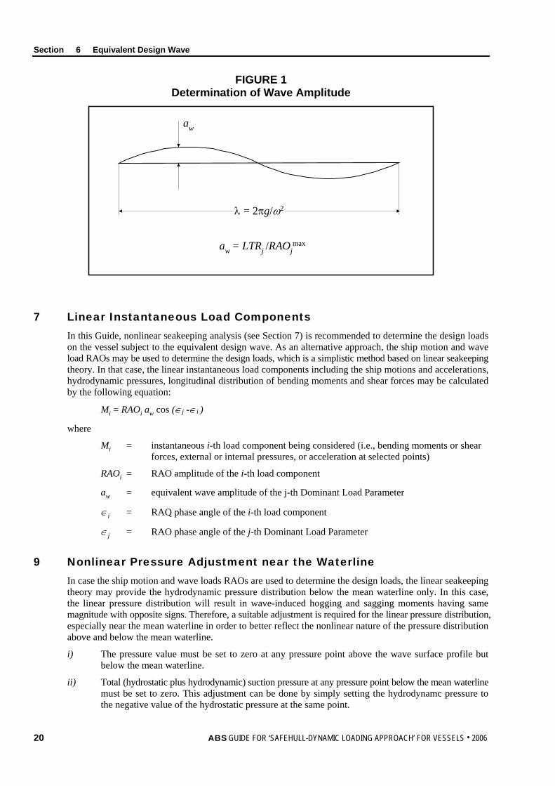
1 General An equivalent design wave is a regular wave that simulates the long-term extreme value of the Dominant Load Parameter under consideration. The equivalent design wave can be characterized by wave amplitude, wave length, wave heading, and wave crest position referenced to the amidships. For each of the Dominant Load Parameters described in Subsection 2/7, an equivalent design wave is to be determined.
Simultaneous load components acting on the hull structure are to be generated for that design wave at the specific time instant when the corresponding Dominant Load Parameter reaches its maximum.
3 Equivalent Wave Amplitude The wave amplitude of the equivalent design wave is to be determined from the long-term extreme value of a Dominant Load Parameter under consideration divided by the maximum RAO amplitude of that Dominant Load Parameter. The maximum RAO occurs at a specific wave frequency and wave heading where the RAO has its maximum value (see Subsection 4/7). Equivalent wave amplitude (EWA) for the j-th Dominant Load Parameter may be expressed by the following equation:
aw = maxj
j
RAO
LTR
where
aw = equivalent wave amplitude of the j-th Dominant Load Parameter
LTRj = long-term response of the j-th Dominant Load Parameter
RAOjmax = maximum RAO amplitude of the j-th Dominant Load Parameter
5 Wave Frequency and Heading The wave frequency and heading of the equivalent design wave, denoted by (, ), are to be determined from the maximum RAO of each Dominant Load Parameter. The wave length of the equivalent design wave can be calculated by the following equation:
= (2g)/2
where
= wave length
g = gravitational acceleration
= wave frequency
Section 6 Equivalent Design Wave
FIGURE 1 Determination of Wave Amplitude
aw
λ = 2πg/ω2
aw = LTRj /RAOjmax
7 Linear Instantaneous Load Components In this Guide, nonlinear seakeeping analysis (see Section 7) is recommended to determine the design loads on the vessel subject to the equivalent design wave. As an alternative approach, the ship motion and wave load RAOs may be used to determine the design loads, which is a simplistic method based on linear seakeeping theory. In that case, the linear instantaneous load components including the ship motions and accelerations, hydrodynamic pressures, longitudinal distribution of bending moments and shear forces may be calculated by the following equation:
Mi = RAOi aw cos (∈j -∈i )
where
Mi = instantaneous i-th load component being considered (i.e., bending moments or shear forces, external or internal pressures, or acceleration at selected points)
RAOi = RAO amplitude of the i-th load component
aw = equivalent wave amplitude of the j-th Dominant Load Parameter
∈i = RAQ phase angle of the i-th load component
∈j = RAO phase angle of the j-th Dominant Load Parameter
9 Nonlinear Pressure Adjustment near the Waterline In case the ship motion and wave loads RAOs are used to determine the design loads, the linear seakeeping theory may provide the hydrodynamic pressure distribution below the mean waterline only. In this case, the linear pressure distribution will result in wave-induced hogging and sagging moments having same magnitude with opposite signs. Therefore, a suitable adjustment is required for the linear pressure distribution, especially near the mean waterline in order to better reflect the nonlinear nature of the pressure distribution above and below the mean waterline.
i) The pressure value must be set to zero at any pressure point above the wave surface profile but below the mean waterline.
ii) Total (hydrostatic plus hydrodynamic) suction pressure at any pressure point below the mean waterline must be set to zero. This adjustment can be done by simply setting the hydrodynamc pressure to the negative value of the hydrostatic pressure at the same point.
20 ABS GUIDE FOR ‘SAFEHULL-DYNAMIC LOADING APPROACH’ FOR VESSELS . 2006
Section 6 Equivalent Design Wave
ABS GUIDE FOR ‘SAFEHULL-DYNAMIC LOADING APPROACH’ FOR VESSELS . 2006 21
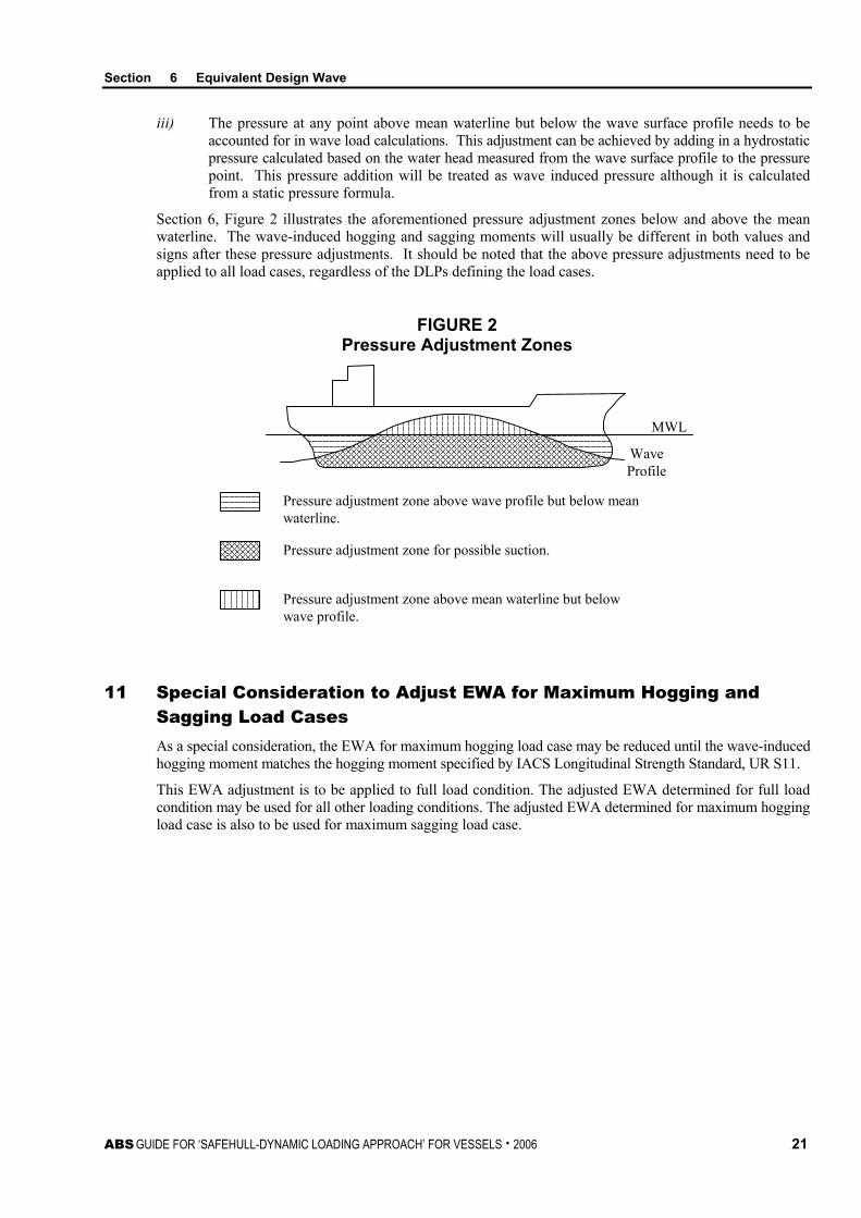
iii) The pressure at any point above mean waterline but below the wave surface profile needs to be accounted for in wave load calculations. This adjustment can be achieved by adding in a hydrostatic pressure calculated based on the water head measured from the wave surface profile to the pressure point. This pressure addition will be treated as wave induced pressure although it is calculated from a static pressure formula.
Section 6, Figure 2 illustrates the aforementioned pressure adjustment zones below and above the mean waterline. The wave-induced hogging and sagging moments will usually be different in both values and signs after these pressure adjustments. It should be noted that the above pressure adjustments need to be applied to all load cases, regardless of the DLPs defining the load cases.
FIGURE 2 Pressure Adjustment Zones
Pressure adjustment zone above wave profile but below meanwaterline.
Pressure adjustment zone for possible suction.
Pressure adjustment zone above mean waterline but belowwave profile.
MWL
WaveProfile
11 Special Consideration to Adjust EWA for Maximum Hogging and Sagging Load Cases As a special consideration, the EWA for maximum hogging load case may be reduced until the wave-induced hogging moment matches the hogging moment specified by IACS Longitudinal Strength Standard, UR S11.
This EWA adjustment is to be applied to full load condition. The adjusted EWA determined for full load condition may be used for all other loading conditions. The adjusted EWA determined for maximum hogging load case is also to be used for maximum sagging load case.
S e c t i o n 7 : N o n l i n e a r S h i p M o t i o n a n d W a v e L o a d
S E C T I O N 7 Nonlinear Ship Motion and Wave Load
1 General For the equivalent design waves defined in Section 6, a nonlinear seakeeping analysis may be performed to calculate the nonlinear ship motions and wave loads. In this Guide, nonlinear time-domain seakeeping analysis is recommended to effectively account for instantaneous nonlinear effects during the time simulation. ABS NLOAD3D or equivalent computer programs may be used to perform these calculations.
3 Nonlinear Seakeeping Analysis
3.1 Concept Under the severe design wave conditions, the ship motions and wave loads are expected to be highly nonlinear, mainly due to the hydrodynamic interaction of the incident waves with the hull geometry above the mean waterline.
Linear seakeeping analysis considers only the hull geometry below the mean waterline as a linear approximation. Nonlinear seakeeping analysis, as a minimum requirement, is to consider the hull geometry above the mean waterline in consideration of:
i) Nonlinear hydrostatic restoring force, and
ii) Nonlinear Froude-Krylov force
which are acting on the instantaneous wetted hull surface below the exact wave surface at every time step during the time simulation.
3.3 Benefits of Nonlinear Seakeeping Analysis In general, linear seakeeping analysis provides hydrodynamic pressure on the hull surface below the mean waterline only. The linear hydrodynamic pressure will give the wave-induced hogging and sagging moments with same magnitudes but opposite signs. Therefore, an appropriate nonlinear correction on the hydrodynamic pressure is required to be used as hydrodynamic loadings for DLA analysis. In the DLA based on linear seakeeping analysis, a quasi-static wave profile correction (described in Subsection 6/11) is required to adjust the pressure distribution near the mean waterline.
In the advanced DLA analysis based on nonlinear seakeeping analysis, however, the quasi-static wave profile correction is not required. The instantaneous nonlinear hydrostatic and Froude-Krylov forces are directly accounted for during the time simulation, which provides a more accurate calculation of the hydrodynamic pressure distribution on the actual wetted surface.
5 Modeling Consideration
5.1 Mathematical Model For the nonlinear seakeeping analysis in time domain, two alternative mathematical formulations may be used: the mixed-source formulation and the Rankine source formulation. The mixed-source formulation requires a matching surface, which is the outer surface surrounding the hull and free surfaces. In the mixed-source formulation, the inner fluid domain inside the matching surface is formulated by a Rankine source, while the outer fluid domain outside the matching surface is formulated by a transient Green function. The velocity potentials of the inner and outer domains should be continuous at the matching surface.
22 ABS GUIDE FOR ‘SAFEHULL-DYNAMIC LOADING APPROACH’ FOR VESSELS . 2006
Section 7 Nonlinear Ship Motion and Wave Load
The Rankine source formulation requires Rankine source distribution on the hull and free surfaces only. The Rankine source formulation requires a numerical damping beach around the outer edge of the free surface in order to absorb the outgoing waves generated by the hull. The size and strength of the damping beach are to be determined to effectively absorb the outgoing waves with a broad range of wave frequencies.
The Rankine source formulation may require larger free surface domain than the mixed-source formulation. The entire free surface domain of the Rankine source formulation is to be at least four times the ship length, including the damping beach. In terms of computational effort, however, the Rankine source formulation can be more efficient than the mixed-source formulation because it does not require the use of the time-consuming transient Green function on the matching surface
5.3 Numerical Course-keeping Model For the time-domain seakeeping analysis, a numerical course-keeping model is required for the simulation of surge, sway and yaw motions. In general, the surge, sway and yaw motions of the vessel occur in the horizontal plane where there exists no hydrostatic restoring force or moment. Without any restoring mechanism, the time simulation of the surge, sway and yaw motions may result in drift motions due to any small transient disturbances or drift forces. In order to prevent unrealistic drift motions in the horizontal plane, a numerical course-keeping model is to be introduced for the motion simulation in time domain.
As a numerical course-keeping model, a rudder-control system or soft-spring system may be used. The rudder-control system based on a simple proportional, integral and derivative (PID) control algorithm may be used to control the rudder angle during the motion simulation. This system may be effective for a vessel cruising at the design speed in moderate sea states. However, for a vessel operating in design wave conditions at reduced ship speed, the rudder-control system is likely to get saturated with subsequent loss of control.
The numerical soft springs are similar to the soft springs used in the experimental setup connecting a model to the towing carriage. These springs are to provide restoring forces and moments sufficient to prevent large drift motion of the model without affecting the wave-induced ship motions. The stiffness of the soft spring is determined so that the natural frequencies of surge, sway and yaw modes fall far below the wave frequency range. Unlike the rudder-control system, the soft-spring system can be more reliable and effective in the extreme design wave conditions.
7 Nonlinear Instantaneous Load Components From the nonlinear seakeeping analysis, the nonlinear instantaneous ship motions and wave loads are to be determined at the instant when each DLP under consideration reaches its maximum.
The ship motions are to include all six degrees-of-freedom rigid-body motions. Depending on the type of a vessel under consideration, the following DLPS are to be considered: vertical acceleration at bow, lateral acceleration at bow, and roll motion (see Subsection 2/7).
The wave loads are the sectional loads acting on the hull along the ship length. The nonlinear wave loads are obtained by integrating the nonlinear hydrostatic and hydrodynamic pressure acting on the instantaneous wetted hull surface and the inertial forces acting on the mass distribution of the cargo and lightship structure along the ship length. Depending on the type of a vessel under consideration, the following DLPs are to be considered: vertical bending moment amidships, horizontal bending moment amidships, vertical shear force at two locations, and torsional moments at five locations along the ship length (see Subsection 2/7).
To determine the nonlinear instantaneous load components accompanying the DLP, a specific instant of time is to be selected when the DLP under consideration reaches its maximum from the response time history of the DLP. The duration of time simulation is to be sufficiently long enough so that the response of the DLP reaches a steady state. It is recommended that the time simulation length be longer than twenty response cycles and the first half of the time history be treated as transient response.
ABS GUIDE FOR ‘SAFEHULL-DYNAMIC LOADING APPROACH’ FOR VESSELS . 2006 23

S e c t i o n 8 : E x t e r n a l P r e s s u r e
S E C T I O N 8 External Pressure
1 General The external hydrodynamic pressures on the wetted hull surface are to be calculated for each Load Case defined by the DLP under consideration (see Subsection 2/7). The external hydrodynamic pressure is to include the pressure components due to waves and the components due to vessel motion.
3 Simultaneously-acting External Pressures For each Load Case, the simultaneously-acting external pressures accompanying the DLP are to be calculated at the specific time instant when the DLP reaches its maximum value. The simultaneously-acting pressures are to be calculated from the linear seakeeping analysis with nonlinear pressure adjustments (see Subsections 6/9 and 6/11) or directly from the nonlinear seakeeping analysis (see Section 7).
5 Pressure Loading on the Structural FE Model The pressure distribution over the hydrodynamic panel model may be too coarse to be used in the structural FE analysis. Therefore, it is necessary to interpolate the pressure over the finer structural mesh. Hydrodynamic pressure may be linearly interpolated to obtain the pressures at each node of the structural FE analysis model.
Section 8, Figure 1 shows an example of the external hydrodynamic pressure distribution mapped on the structural FE model of a container carrier. The pressure distribution is a simultaneously-acting pressure accompanying the DLP of maximum hogging moment amidships at the instant time when the DLP reaches its maximum.
The external pressure distribution mapped over the structural FE model should contain both hydrostatic and hydrodynamic pressures.
FIGURE 1 Sample External Hydrodynamic Pressure for Maximum Hogging Moment Amidships
24 ABS GUIDE FOR ‘SAFEHULL-DYNAMIC LOADING APPROACH’ FOR VESSELS . 2006
S e c t i o n 9 : I n t e r n a l L i q u i d T a n k P r e s s u r e
S E C T I O N 9 Internal Liquid Tank Pressure
1 General The internal pressures acting on the internal surfaces of liquid cargo and ballast tanks are to be calculated and applied to the structural FE model for DLA analysis. Static and dynamic pressures on completely filled and/or partially filled tanks are to be considered in the analysis. Tank sloshing loads are not included in DLA analysis. These sloshing loads are to be treated in accordance with the current Rule requirements
3 Pressure Components The internal liquid tank pressure is composed of static and dynamic components. The static pressure component results from gravity. The dynamic pressure component can be further decomposed into quasi-static and inertial components. The quasi-static component results from gravity due to roll and pitch inclinations of the tank. The direction of gravitational forces in the ship-fixed coordinate system varies with roll and pitch motion, resulting in a change of internal pressure.
The inertial component results from the instantaneous local accelerations of the tank content (liquid cargo or ballast) caused by the ship motions in six degrees of freedom. In the procedure, the vertical, transverse and longitudinal accelerations due to the ship motion are defined in the ship-fixed coordinate system. Therefore, transformation of the acceleration to the ship system due to roll and pitch inclinations is not needed.
The internal tank pressure for each of the tank boundary points can be calculated from the following equation, which is expressed in a combined formula of the static and dynamic pressure components:
p = po + ρ hi [(g + aV)2 + (gT + aT)2 + (gL + aL)2 ]1/2
where
p = internal tank pressure at a tank boundary point
po = either the vapor pressure or the pressure setting on pressure/vacuum relief valve
ρ = liquid density, cargo or ballast
hi = internal pressure head defined by the height of projected liquid column in the direction of a resultant acceleration vector. For a completely filled tank, the pressure head is to be measured from the highest point of the tank to the load point (see Section 9, Figure 1). For a partially filled tank, the pressure head is to be measured from the free surface level to the load point (see Section 9, Figure 2). The free surface is defined as the liquid surface normal to the resultant acceleration vector. In the above figures, only vertical and transverse accelerations are considered for illustration purpose.
g = acceleration of gravity
gL, gT = longitudinal and transverse components of gravitational acceleration relative to the ship-fixed coordinate system due to roll and pitch inclinations
= (–g sin φ, g sin θ)
θ = roll angle
φ = pitch angle
aL, aT, aV = longitudinal, transverse and vertical components of local accelerations caused by ship motions relative to the ship-fixed coordinate system at the center of gravity of tank contents
ABS GUIDE FOR ‘SAFEHULL-DYNAMIC LOADING APPROACH’ FOR VESSELS . 2006 25
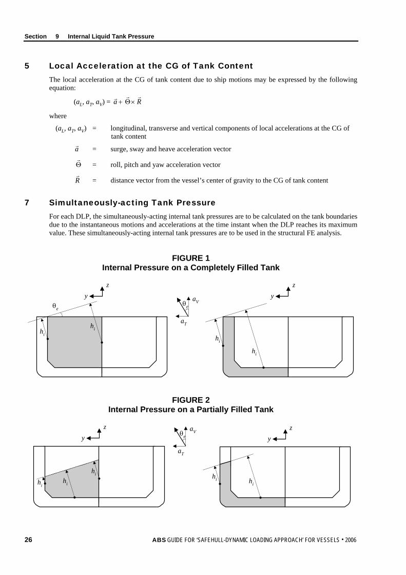
Section 9 Internal Liquid Tank Pressure
5 Local Acceleration at the CG of Tank Content The local acceleration at the CG of tank content due to ship motions may be expressed by the following equation:
(aL, aT, aV) = Ra
×Θ+
where
(aL, aT, aV) = longitudinal, transverse and vertical components of local accelerations at the CG of tank content
a = surge, sway and heave acceleration vector
Θ
= roll, pitch and yaw acceleration vector
R
= distance vector from the vessel’s center of gravity to the CG of tank content
7 Simultaneously-acting Tank Pressure For each DLP, the simultaneously-acting internal tank pressures are to be calculated on the tank boundaries due to the instantaneous motions and accelerations at the time instant when the DLP reaches its maximum value. These simultaneously-acting internal tank pressures are to be used in the structural FE analysis.
FIGURE 1 Internal Pressure on a Completely Filled Tank
yz
aT
aVθeθe
hi
hi
yz
hi
hi
FIGURE 2 Internal Pressure on a Partially Filled Tank
yz
aT
aVθe
hi
hihi
yz
hi hi
26 ABS GUIDE FOR ‘SAFEHULL-DYNAMIC LOADING APPROACH’ FOR VESSELS . 2006
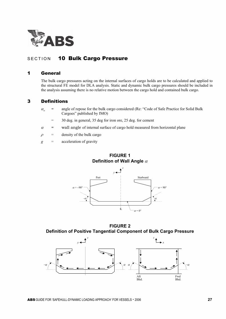
ABS GUIDE FOR ‘SAFEHULL-DYNAMIC LOADING APPROACH’ FOR VESSELS . 2006 27
S e c t i o n 1 0 : B u l k C a r g o P r e s s u r e
S E C T I O N 10 Bulk Cargo Pressure
1 General The bulk cargo pressures acting on the internal surfaces of cargo holds are to be calculated and applied to the structural FE model for DLA analysis. Static and dynamic bulk cargo pressures should be included in the analysis assuming there is no relative motion between the cargo hold and contained bulk cargo.
3 Definitions o = angle of repose for the bulk cargo considered (Re: “Code of Safe Practice for Solid Bulk
Cargoes” published by IMO)
= 30 deg. in general, 35 deg for iron ore, 25 deg. for cement
= wall angle of internal surface of cargo hold measured from horizontal plane
= density of the bulk cargo
g = acceleration of gravity
FIGURE 1 Definition of Wall Angle
LC
= 90°
= 0°
Starboard
= 90°
Port
y
z
FIGURE 2 Definition of Positive Tangential Component of Bulk Cargo Pressure
y
z
x
z
AftBhd.
FwdBhd.
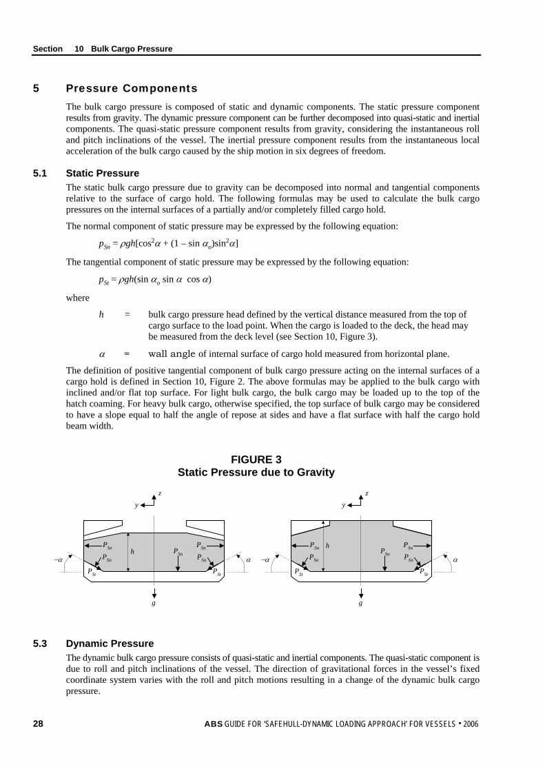
Section 10 Bulk Cargo Pressure
5 Pressure Components The bulk cargo pressure is composed of static and dynamic components. The static pressure component results from gravity. The dynamic pressure component can be further decomposed into quasi-static and inertial components. The quasi-static pressure component results from gravity, considering the instantaneous roll and pitch inclinations of the vessel. The inertial pressure component results from the instantaneous local acceleration of the bulk cargo caused by the ship motion in six degrees of freedom.
5.1 Static Pressure The static bulk cargo pressure due to gravity can be decomposed into normal and tangential components relative to the surface of cargo hold. The following formulas may be used to calculate the bulk cargo pressures on the internal surfaces of a partially and/or completely filled cargo hold.
The normal component of static pressure may be expressed by the following equation:
pSn = ρgh[cos2α + (1 – sin αo)sin2α]
The tangential component of static pressure may be expressed by the following equation:
pSt = ρgh(sin αo sin α cos α)
where
h = bulk cargo pressure head defined by the vertical distance measured from the top of cargo surface to the load point. When the cargo is loaded to the deck, the head may be measured from the deck level (see Section 10, Figure 3).
α = wall angle of internal surface of cargo hold measured from horizontal plane.
The definition of positive tangential component of bulk cargo pressure acting on the internal surfaces of a cargo hold is defined in Section 10, Figure 2. The above formulas may be applied to the bulk cargo with inclined and/or flat top surface. For light bulk cargo, the bulk cargo may be loaded up to the top of the hatch coaming. For heavy bulk cargo, otherwise specified, the top surface of bulk cargo may be considered to have a slope equal to half the angle of repose at sides and have a flat surface with half the cargo hold beam width.
FIGURE 3 Static Pressure due to Gravity
PSn
PSn
PSn
PSt
α
g
yz
hPSn
PSn
PSt
−αPSn
PSn
PSn
PSt
α
g
yz
hPSn
PSn
PSt
−α
5.3 Dynamic Pressure The dynamic bulk cargo pressure consists of quasi-static and inertial components. The quasi-static component is due to roll and pitch inclinations of the vessel. The direction of gravitational forces in the vessel’s fixed coordinate system varies with the roll and pitch motions resulting in a change of the dynamic bulk cargo pressure.
28 ABS GUIDE FOR ‘SAFEHULL-DYNAMIC LOADING APPROACH’ FOR VESSELS . 2006
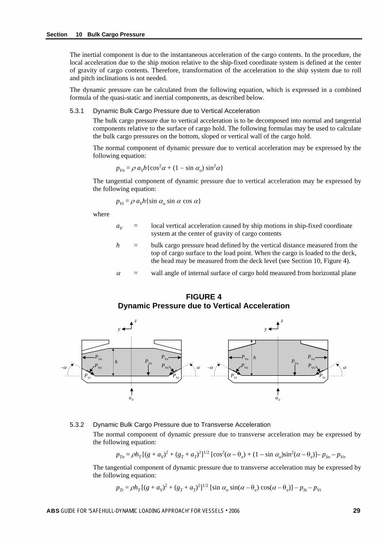
Section 10 Bulk Cargo Pressure
The inertial component is due to the instantaneous acceleration of the cargo contents. In the procedure, the local acceleration due to the ship motion relative to the ship-fixed coordinate system is defined at the center of gravity of cargo contents. Therefore, transformation of the acceleration to the ship system due to roll and pitch inclinations is not needed.
The dynamic pressure can be calculated from the following equation, which is expressed in a combined formula of the quasi-static and inertial components, as described below.
5.3.1 Dynamic Bulk Cargo Pressure due to Vertical Acceleration The bulk cargo pressure due to vertical acceleration is to be decomposed into normal and tangential components relative to the surface of cargo hold. The following formulas may be used to calculate the bulk cargo pressures on the bottom, sloped or vertical wall of the cargo hold.
The normal component of dynamic pressure due to vertical acceleration may be expressed by the following equation:
pVn = ρ aVh{cos2α + (1 − sin αo) sin2α}
The tangential component of dynamic pressure due to vertical acceleration may be expressed by the following equation:
pVt = ρ aVh{sin αo sin α cos α}
where
aV = local vertical acceleration caused by ship motions in ship-fixed coordinate system at the center of gravity of cargo contents
h = bulk cargo pressure head defined by the vertical distance measured from the top of cargo surface to the load point. When the cargo is loaded to the deck, the head may be measured from the deck level (see Section 10, Figure 4).
α = wall angle of internal surface of cargo hold measured from horizontal plane
FIGURE 4 Dynamic Pressure due to Vertical Acceleration
PVn
PVn
PVn
PVt
α
aV
yz
hPVn
PVn
PVt
−αPVn
PVn
PVn
PVt
α
aV
yz
hPVn
PVn
PVt
−α
5.3.2 Dynamic Bulk Cargo Pressure due to Transverse Acceleration The normal component of dynamic pressure due to transverse acceleration may be expressed by the following equation:
pTn = ρhT [(g + aV)2 + (gT + aT)2]1/2 [cos2(α – θe) + (1 – sin αo)sin2(α – θe)]– pSn – pVn
The tangential component of dynamic pressure due to transverse acceleration may be expressed by the following equation:
pTt = ρhT [(g + aV)2 + (gT + aT)2]1/2 [sin αo sin(α – θe) cos(α – θe)] – pSt – pVt
ABS GUIDE FOR ‘SAFEHULL-DYNAMIC LOADING APPROACH’ FOR VESSELS . 2006 29
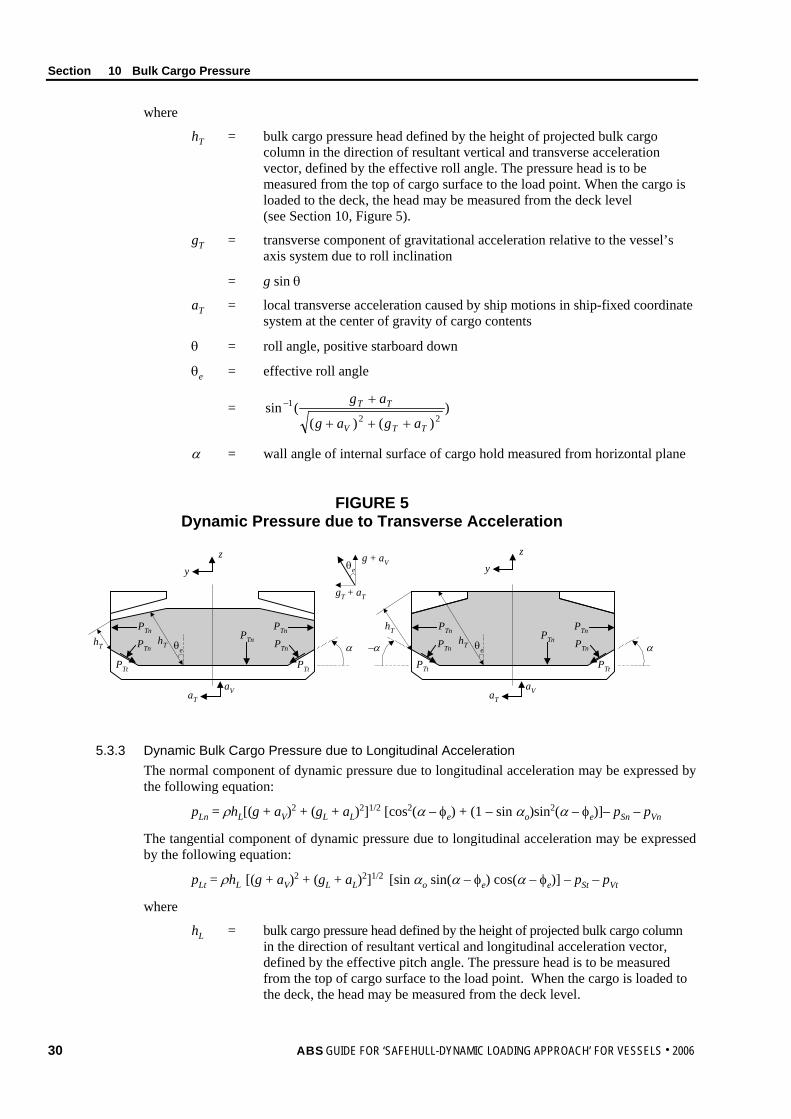
Section 10 Bulk Cargo Pressure
where
hT = bulk cargo pressure head defined by the height of projected bulk cargo column in the direction of resultant vertical and transverse acceleration vector, defined by the effective roll angle. The pressure head is to be measured from the top of cargo surface to the load point. When the cargo is loaded to the deck, the head may be measured from the deck level (see Section 10, Figure 5).
gT = transverse component of gravitational acceleration relative to the vessel’s axis system due to roll inclination
= g sin θ
aT = local transverse acceleration caused by ship motions in ship-fixed coordinate system at the center of gravity of cargo contents
θ = roll angle, positive starboard down
θe = effective roll angle
= ))()(
(sin22
1
TTV
TT
agag
ag
+++
+−
α = wall angle of internal surface of cargo hold measured from horizontal plane
FIGURE 5 Dynamic Pressure due to Transverse Acceleration
PTn
PTn
PTn
PTt
α
aT
yz
aV
gT + aT
g + aVθe
θehT
PTn
PTn
PTt
hTPTn
PTn
PTn
PTt
α
yz
PTn
PTn
PTt
−α
hT
θehT
aT
aV
5.3.3 Dynamic Bulk Cargo Pressure due to Longitudinal Acceleration The normal component of dynamic pressure due to longitudinal acceleration may be expressed by the following equation:
pLn = ρhL[(g + aV)2 + (gL + aL)2]1/2 [cos2(α – φe) + (1 – sin αo)sin2(α – φe)]– pSn – pVn
The tangential component of dynamic pressure due to longitudinal acceleration may be expressed by the following equation:
pLt = ρhL [(g + aV)2 + (gL + aL)2]1/2 [sin αo sin(α – φe) cos(α – φe)] – pSt – pVt
where
hL = bulk cargo pressure head defined by the height of projected bulk cargo column in the direction of resultant vertical and longitudinal acceleration vector, defined by the effective pitch angle. The pressure head is to be measured from the top of cargo surface to the load point. When the cargo is loaded to the deck, the head may be measured from the deck level.
30 ABS GUIDE FOR ‘SAFEHULL-DYNAMIC LOADING APPROACH’ FOR VESSELS . 2006
Section 10 Bulk Cargo Pressure
gL = longitudinal component of gravitational acceleration relative to the vessel’s axis system due to pitch inclination
= –g sin φ
aL = local longitudinal acceleration caused by ship motions in ship-fixed coordinate system at the center of gravity of cargo contents
φ = pitch angle
φe = effective pitch angle,
=
+++
+−
22
1
)()(sin
LLV
LL
agag
ag
α = wall angle of internal surface of cargo hold measured from horizontal plane
7 Local Acceleration at the CG of Tank Content The local acceleration at the CG of tank content due to ship motions may be expressed by the following equation:
(aL, aT, aV) = Ra
×Θ+
where
(aL, aT, aV) = longitudinal, transverse and vertical components of local accelerations at the CG of tank content
a = surge, sway and heave acceleration vector
Θ
= roll, pitch and yaw acceleration vector
R
= distance vector from the vessel’s center of gravity to the CG of tank content
9 Simultaneously-acting Bulk Cargo Load For each DLP, the simultaneously-acting static and dynamic bulk cargo pressures are to be calculated on the cargo hold boundaries due to the instantaneous motions and accelerations at the time instant when the DLP reaches its maximum value. These simultaneously-acting bulk cargo pressures are to be used in the structural FE analysis.
ABS GUIDE FOR ‘SAFEHULL-DYNAMIC LOADING APPROACH’ FOR VESSELS . 2006 31
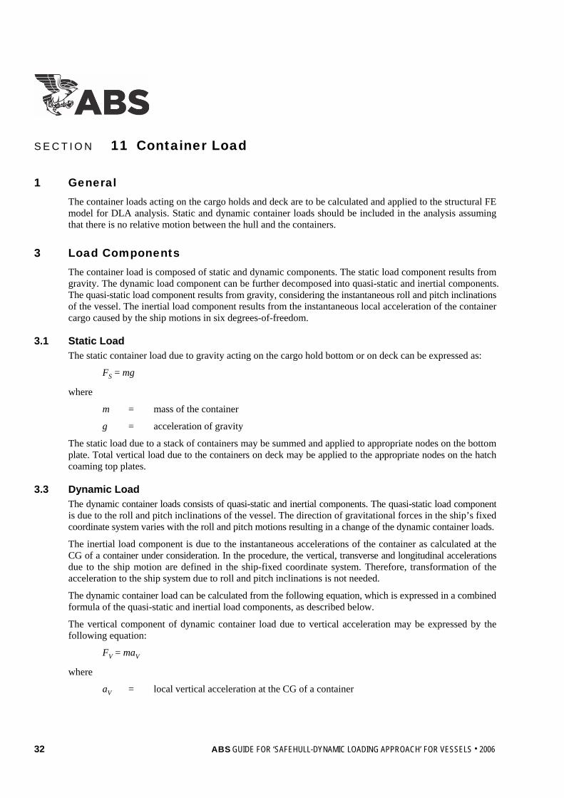
S e c t i o n 1 1 : C o n t a i n e r L o a d
S E C T I O N 11 Container Load
1 General The container loads acting on the cargo holds and deck are to be calculated and applied to the structural FE model for DLA analysis. Static and dynamic container loads should be included in the analysis assuming that there is no relative motion between the hull and the containers.
3 Load Components The container load is composed of static and dynamic components. The static load component results from gravity. The dynamic load component can be further decomposed into quasi-static and inertial components. The quasi-static load component results from gravity, considering the instantaneous roll and pitch inclinations of the vessel. The inertial load component results from the instantaneous local acceleration of the container cargo caused by the ship motions in six degrees-of-freedom.
3.1 Static Load The static container load due to gravity acting on the cargo hold bottom or on deck can be expressed as:
FS = mg
where
m = mass of the container
g = acceleration of gravity
The static load due to a stack of containers may be summed and applied to appropriate nodes on the bottom plate. Total vertical load due to the containers on deck may be applied to the appropriate nodes on the hatch coaming top plates.
3.3 Dynamic Load The dynamic container loads consists of quasi-static and inertial components. The quasi-static load component is due to the roll and pitch inclinations of the vessel. The direction of gravitational forces in the ship’s fixed coordinate system varies with the roll and pitch motions resulting in a change of the dynamic container loads.
The inertial load component is due to the instantaneous accelerations of the container as calculated at the CG of a container under consideration. In the procedure, the vertical, transverse and longitudinal accelerations due to the ship motion are defined in the ship-fixed coordinate system. Therefore, transformation of the acceleration to the ship system due to roll and pitch inclinations is not needed.
The dynamic container load can be calculated from the following equation, which is expressed in a combined formula of the quasi-static and inertial load components, as described below.
The vertical component of dynamic container load due to vertical acceleration may be expressed by the following equation:
FV = maV
where
aV = local vertical acceleration at the CG of a container
32 ABS GUIDE FOR ‘SAFEHULL-DYNAMIC LOADING APPROACH’ FOR VESSELS . 2006
Section 11 Container Load
The transverse component of dynamic container load due to transverse acceleration may be expressed by the following equation:
FT = m(gT + aT)
where
gT = transverse component of gravitational acceleration relative to the vessel’s axis system due to roll inclination
= g sin θ
aT = local transverse acceleration at the CG of a container
The transverse load due to containers may be distributed to appropriate nodes on the bulkhead structure via the container cell guide. The total transverse load due to the containers on deck may be applied to the appropriate nodes on the hatch coaming top plates via the container lashing system.
The longitudinal component of dynamic container load due to longitudinal acceleration may be expressed by the following equation:
FL = m(gL + aL)
where
gL = longitudinal component of gravitational acceleration relative to the vessel’s axis system due to pitch inclination
= –g sin φ
aL = local longitudinal acceleration at the CG of a container
FIGURE 1 Dynamic Load due to Vertical and Transverse Acceleration
FV
FT∇∇
aT
aV
5 Local Acceleration at the CG of a Container The local acceleration at the CG of a container due to ship motions may be expressed by the following equation:
(aL, aT, aV) = Ra
×Θ+
where
(aL, aT, aV) = longitudinal, transverse and vertical components of local acceleration at the CG of a container
ABS GUIDE FOR ‘SAFEHULL-DYNAMIC LOADING APPROACH’ FOR VESSELS . 2006 33

Section 11 Container Load
a = surge, sway and heave acceleration vector
Θ
= roll, pitch and yaw acceleration vector
R
= distance vector from the vessel’s center of gravity to the CG of a container
7 Simultaneously-acting Container Load For each DLP, the simultaneously-acting static and dynamic container loads are to be calculated on the cargo hold and deck due to the instantaneous motions and accelerations at the time instant when the DLP reaches its maximum value. These simultaneously-acting container loads are to be used in the structural FE analysis.
34 ABS GUIDE FOR ‘SAFEHULL-DYNAMIC LOADING APPROACH’ FOR VESSELS . 2006
S e c t i o n 1 2 : L o a d o n L i g h t s h i p S t r u c t u r e a n d E q u i p m e n t
S E C T I O N 12 Load on Lightship Structure and Equipment
1 General The static and dynamic loads acting on the lightship structure and equipment are to be calculated and applied to the structural FE model for DLA analysis.
3 Load Components The load on lightship structure and equipment is composed of static and dynamic components. The static load results from gravity. The dynamic load can be further decomposed into quasi-static and inertial components. The quasi-static load results from gravity, considering the instantaneous roll and pitch inclinations of the vessel. The inertial load results from the instantaneous local accelerations on the lightship structure and equipment caused by the ship motions in six degrees-of-freedom.
3.1 Static Load The static load due to gravity acting on the lightship structure and equipments can be expressed as:
FS = mg
where
m = nodal mass of the structural member or equipment
g = acceleration of gravity
3.3 Dynamic Load The dynamic load consists of quasi-static and inertial components. The quasi-static load is due to the roll and pitch inclinations of the vessel. The direction of gravitational forces in the ship’s fixed coordinate system varies with the roll and pitch motions resulting in a change of the dynamic load.
The inertial load is due to the instantaneous local acceleration on the lightship structure and equipment. In the procedure, the vertical, transverse and longitudinal components of local accelerations are defined in the ship-fixed coordinate system.
The dynamic load can be calculated from the following equation, which is expressed in a combined formula of the quasi-static and inertial components, as described below.
The vertical component of dynamic load due to vertical acceleration may be expressed by the following equation:
FV = maV
where
aV = local vertical acceleration
ABS GUIDE FOR ‘SAFEHULL-DYNAMIC LOADING APPROACH’ FOR VESSELS . 2006 35
Section 12 Load on Lightship Structure and Equipment
The transverse component of dynamic load due to transverse acceleration may be expressed by the following equation:
FT = m(gT + aT)
where
gT = transverse component of gravitational acceleration relative to the ship-fixed coordinate system due to roll inclination
= g sin θ
aT = local transverse acceleration
The longitudinal component of dynamic load due to longitudinal acceleration may be expressed by the following equation:
FL = m(gL + aL)
where
gL = longitudinal component of gravitational acceleration relative to the ship-fixed coordinate system due to pitch inclination
= –g sin φ
aL = local longitudinal acceleration
5 Local Acceleration The local acceleration at a location of interest may be expressed by the following equation:
(aL, aT, aV) = Ra
×Θ+
where
(aL, aT, aV) = longitudinal, transverse and vertical components of local acceleration
a = surge, sway and heave acceleration vector
Θ
= roll, pitch and yaw acceleration vector
R
= distance vector from the vessel’s center of gravity to the location of interest
7 Simultaneously-acting Loads on Lightship Structure and Equipment For each DLP, the simultaneously-acting static and dynamic loads on lightship structure and equipment are to be calculated at the time instant when the DLP under consideration reaches its maximum value. These simultaneously-acting inertial loads on the lightship structure and equipment are to be applied to each node of the structural FE model in the structural analysis.
36 ABS GUIDE FOR ‘SAFEHULL-DYNAMIC LOADING APPROACH’ FOR VESSELS . 2006
S e c t i o n 1 3 : L o a d i n g f o r S t r u c t u r a l F E A n a l y s i s
S E C T I O N 13 Loading for Structural FE Analysis
1 General For each Load Case, structural loadings are to be applied to the global (whole vessel) structural FE model. The structural loadings are to include both static and dynamic load components determined in accordance with Sections 7, 8 and 9. The static load components are those caused, for example, by buoyancy or gravity, and should be included in the structural FE analysis.
3 Equilibrium Check The model of the hull girder structure is to be in a dynamic equilibrium condition with all load components applied.
The unbalanced forces in the model’s global axis system for each Load Case need to be determined and resolved. The magnitudes of the unbalanced forces and the procedure used to balance the structural model in equilibrium prior to solution should be fully documented.
5 Boundary Forces and Moments When the FE analysis model considers only a portion of the vessel, boundary conditions are required at the end sections of the partial model. These conditions are represented by the instantaneous vertical and lateral shear forces and three moments at the instant of time when the Dominant Load Parameter reaches its maximum. The method to calculate the instantaneous loads is described in Subsection 6/9.
ABS GUIDE FOR ‘SAFEHULL-DYNAMIC LOADING APPROACH’ FOR VESSELS . 2006 37

S e c t i o n 1 4 : S t r u c t u r a l F E A n a l y s i s
S E C T I O N 14 Structural FE Analysis
1 General The structural adequacy of the hull is examined by the finite element (FE) analysis using global and local FE models. The global FE model is recommended to have sufficient mesh density to represent the entire hull girder structure and main supporting members.
For the critical areas with high stress levels, a local FE analysis is recommended using a local finer mesh model representing the structural details. In this case, the results of nodal displacements or forces obtained from the global FE analysis are to be used as boundary conditions in the subsequent local FE analysis.
The DLA strength assessment procedures in this Guide are based on the “gross” ship approach, which uses the gross or as-built scantlings in the FE modeling. For more details of global FE modeling, refer to the ABS Guidance Notes on SafeHull Finite Element Analysis of Hull Structures.
3 Global FE Analysis The overall structural responses of the vessels are to be determined by the global FE analysis applying the instantaneous load components for each Load Case. The global FE analysis is to consider the structural responses of the entire hull girder and main supporting members. Typically a one-longitudinal spacing mesh size is recommended for global FE models.
In making the global 3D FE model, a judicious selection of nodes, elements and degrees of freedom is to be made to represent the stiffness and inertia properties of the hull structure, while keeping the size of the model and required data generation within manageable limits. Lumping of stiffeners, use of equivalent plate thicknesses and other such techniques may be used for this purpose.
In general, the global FE model, whose geometry, configuration and stiffness approximate the actual hull structure, mainly consists of three types of elements.
i) Truss or rod elements with axial stiffness only
ii) Bar or beam elements with axial, torsional and bending stiffness
iii) Plate elements with in-plane and out-of-plane stiffness in either triangular or quadrilateral shapes.
5 Local FE Analysis For the critical areas where the global FE analysis indicates high stress levels, more detailed local FE analysis is recommended by local finer mesh model, based on the results of the global FE analysis. In this case, boundary displacements obtained from the global FE analysis are to be used as boundary conditions in the fine mesh analysis. In addition to the boundary constraints, the pertinent local loads should be reapplied to the fine mesh models.
The following are the structural components generally regarded as critical areas of vessels.
5.1 Tanker The critical areas of a tanker may include, but not limited to, the following local structures:
i) Transverse web frames
ii) Centerline and off-centerline longitudinal girder structures
iii) Horizontal stringers of watertight transverse bulkheads
iv) Hopper knuckle connections
38 ABS GUIDE FOR ‘SAFEHULL-DYNAMIC LOADING APPROACH’ FOR VESSELS . 2006
Section 14 Structural FE Analysis
5.3 Bulk Carrier The critical areas of a bulk carrier may include, but not limited to, the following local structures:
i) Hatch coamings, side girder and hatch end
ii) Deck plating and longitudinals, plating and stiffeners between hatches
iii) Bottom and inner bottom plating and longitudinals, double bottom floors and girders
iv) Bulkheads
• Longitudinal bulkheads or sloping bulkheads plating and stiffeners
• Transverse bulkhead plating and stiffeners or corrugations
v) Side shell plating, longitudinals and transverse frames
vi) Web frames, transverses, diaphragms, bulkheads in upper and lower wing tanks including web frames in cargo holds
vii) Upper and lower stool structures
5.5 Container Carrier The critical areas of a container carrier may include, but not limited to, the following local structures:
i) Hatch corners and hatch coaming top plates
ii) Deck plating, longitudinal stiffeners and girders
iii) Bottom and inner bottom plating, longitudinal stiffeners and girders
iv) Side shell plating, longitudinal stiffeners
v) Transverse web frames
5.7 LNG Carrier The critical areas of a LNG carrier may include, but not limited to, the following local structures:
i) Transverse web frames
ii) Centerline and off-centerline longitudinal girder structures
iii) Horizontal stringers of watertight transverse bulkheads
iv) Hopper knuckle connections
In making the local finer mesh model, care is to be taken to accurately represent the stiffness of the local structures as well as their geometry, such as the connections, openings, bracket toes and structural knuckle points.
7 Fatigue Assessment Fatigue assessment of the vessels in areas such as hopper knuckles or hatch corners is very important. Spectral fatigue analysis is outside the scope of the DLA analysis. The global and local FE models developed for DLA analysis can be used in spectral fatigue analysis. Detailed procedures for spectral fatigue analysis and the SFA notation are described in the ABS Guide for Spectral-Based Fatigue Analysis for Vessels.
ABS GUIDE FOR ‘SAFEHULL-DYNAMIC LOADING APPROACH’ FOR VESSELS . 2006 39
40 ABS GUIDE FOR ‘SAFEHULL-DYNAMIC LOADING APPROACH’ FOR VESSELS . 2006
S e c t i o n 1 5 : A c c e p t a n c e C r i t e r i a
S E C T I O N 15 Acceptance Criteria
1 General For assessing the results of the finite element analyses, two failure modes of the structure are to be considered:
i) Yielding
ii) Buckling and Ultimate Strength
General guidance on fatigue assessment is contained separately in the ABS Guide for Spectral-Based Fatigue Analysis for Vessels.
The evaluation for yielding and buckling of the main supporting members with high stress level is to be mainly based on the results of local finer mesh models where more accurate structural details are considered.
3 Yielding For a plate element subjected to biaxial stresses, a specific combination of stress components, rather than a single maximum normal stress component constitutes the limiting condition. In this regard, the following equivalent stress, given by the Hencky-von Mises theory, is to be compared to a maximum allowable percentage of the material’s yield strength:
HVM = 222 3 xyyxyx
where
x = normal stress in the x-direction (local axis system of the element)
y = normal stress in the y-direction
xy = shear stress
or using principal stresses, 1 and 2:
HVM = 2122
21
The von Mises stress obtained from the global FE analysis is not to exceed a certain portion of the material’s yield strength. Given the recommended global FE mesh of one longitudinal spacing for hull girder and main supporting members (watertight) and finer local FE mesh for critical areas and structural details such as openings and bracket toes, the resulting stresses may be categorized into the three levels of stresses such as field stress, local stress and hot-spot stress.
3.1 Field Stress Field stresses are indicative of stress severity sufficiently away from structural details such as hopper knuckles, openings and bracket toes. The recommended basic mesh size for capturing field stresses is one longitudinal spacing. Typically, element stresses directly obtained from global 3D FE models of one longitudinal spacing can be considered as field stresses. For main supporting members, field stresses are primarily due to primary hull girder deformation and secondary bending between watertight boundaries.
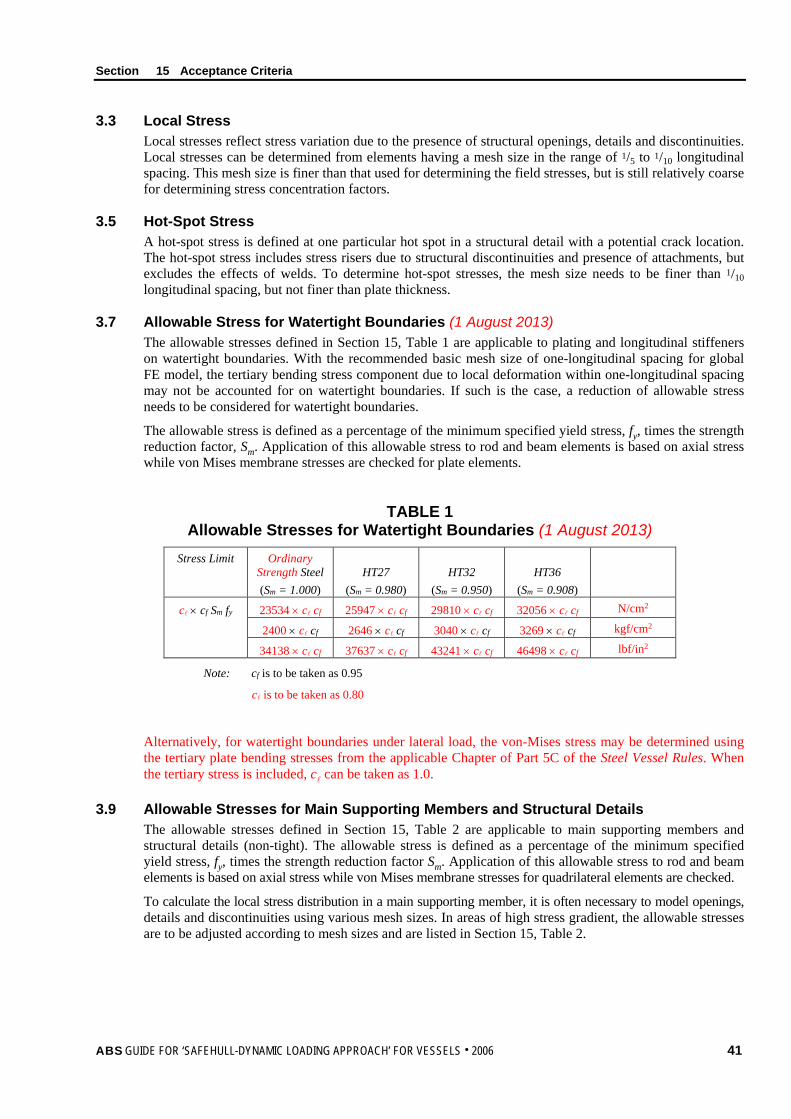
Section 15 Acceptance Criteria
3.3 Local Stress Local stresses reflect stress variation due to the presence of structural openings, details and discontinuities. Local stresses can be determined from elements having a mesh size in the range of 1/5 to 1/10 longitudinal spacing. This mesh size is finer than that used for determining the field stresses, but is still relatively coarse for determining stress concentration factors.
3.5 Hot-Spot Stress A hot-spot stress is defined at one particular hot spot in a structural detail with a potential crack location. The hot-spot stress includes stress risers due to structural discontinuities and presence of attachments, but excludes the effects of welds. To determine hot-spot stresses, the mesh size needs to be finer than 1/10 longitudinal spacing, but not finer than plate thickness.
3.7 Allowable Stress for Watertight Boundaries (1 August 2013) The allowable stresses defined in Section 15, Table 1 are applicable to plating and longitudinal stiffeners on watertight boundaries. With the recommended basic mesh size of one-longitudinal spacing for global FE model, the tertiary bending stress component due to local deformation within one-longitudinal spacing may not be accounted for on watertight boundaries. If such is the case, a reduction of allowable stress needs to be considered for watertight boundaries.
The allowable stress is defined as a percentage of the minimum specified yield stress, fy, times the strength reduction factor, Sm. Application of this allowable stress to rod and beam elements is based on axial stress while von Mises membrane stresses are checked for plate elements.
TABLE 1 Allowable Stresses for Watertight Boundaries (1 August 2013)
Stress Limit Ordinary Strength Steel (Sm = 1.000)
HT27
(Sm = 0.980)
HT32
(Sm = 0.950)
HT36
(Sm = 0.908)
c × cf Sm fy 23534 × c cf 25947 × c cf 29810 × c cf 32056 × c cf N/cm2
2400 × c cf 2646 × c cf 3040 × c cf 3269 × c cf kgf/cm2
34138 × c cf 37637 × c cf 43241 × c cf 46498 × c cf lbf/in2
Note: cf is to be taken as 0.95
c is to be taken as 0.80
Alternatively, for watertight boundaries under lateral load, the von-Mises stress may be determined using the tertiary plate bending stresses from the applicable Chapter of Part 5C of the Steel Vessel Rules. When the tertiary stress is included, c can be taken as 1.0.
3.9 Allowable Stresses for Main Supporting Members and Structural Details The allowable stresses defined in Section 15, Table 2 are applicable to main supporting members and structural details (non-tight). The allowable stress is defined as a percentage of the minimum specified yield stress, fy, times the strength reduction factor Sm. Application of this allowable stress to rod and beam elements is based on axial stress while von Mises membrane stresses for quadrilateral elements are checked.
To calculate the local stress distribution in a main supporting member, it is often necessary to model openings, details and discontinuities using various mesh sizes. In areas of high stress gradient, the allowable stresses are to be adjusted according to mesh sizes and are listed in Section 15, Table 2.
ABS GUIDE FOR ‘SAFEHULL-DYNAMIC LOADING APPROACH’ FOR VESSELS . 2006 41
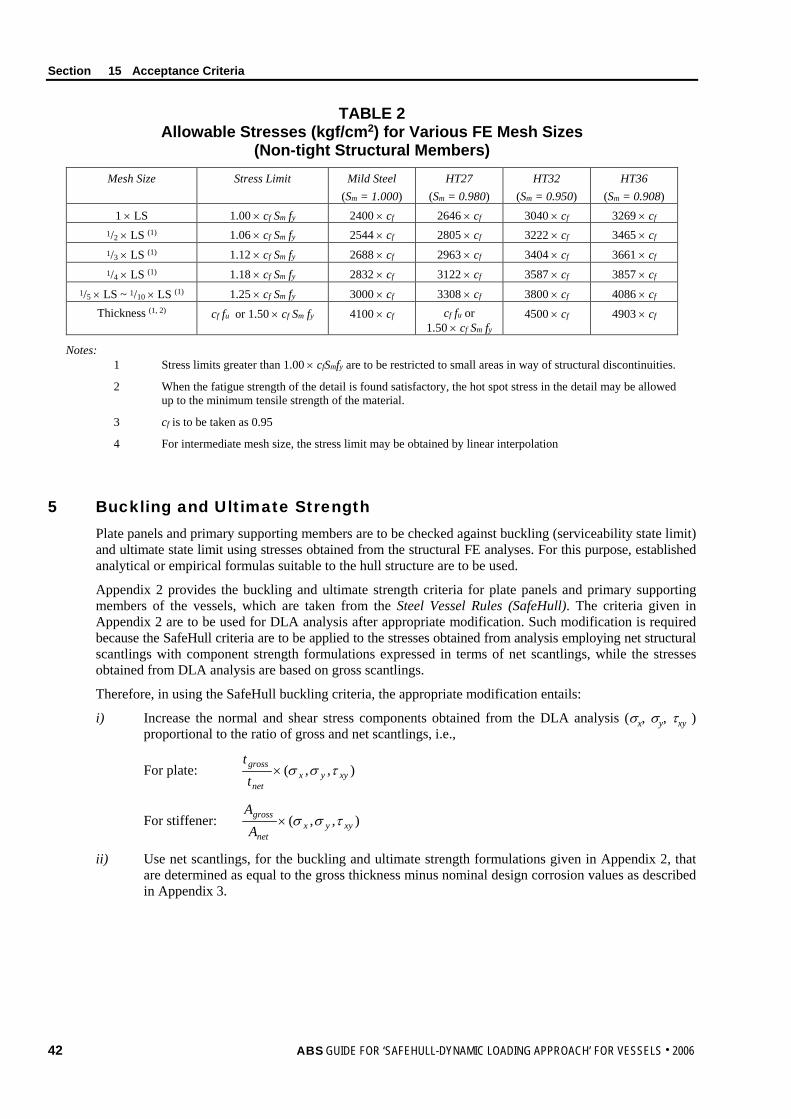
Section 15 Acceptance Criteria
TABLE 2 Allowable Stresses (kgf/cm2) for Various FE Mesh Sizes
(Non-tight Structural Members) Mesh Size Stress Limit Mild Steel
(Sm = 1.000) HT27
(Sm = 0.980) HT32
(Sm = 0.950) HT36
(Sm = 0.908) 1 × LS 1.00 × cf Sm fy 2400 × cf 2646 × cf 3040 × cf 3269 × cf
1/2 × LS (1) 1.06 × cf Sm fy 2544 × cf 2805 × cf 3222 × cf 3465 × cf 1/3 × LS (1) 1.12 × cf Sm fy 2688 × cf 2963 × cf 3404 × cf 3661 × cf 1/4 × LS (1) 1.18 × cf Sm fy 2832 × cf 3122 × cf 3587 × cf 3857 × cf
1/5 × LS ~ 1/10 × LS (1) 1.25 × cf Sm fy 3000 × cf 3308 × cf 3800 × cf 4086 × cf Thickness (1, 2) cf fu or 1.50 × cf Sm fy 4100 × cf cf fu or
1.50 × cf Sm fy 4500 × cf 4903 × cf
Notes: 1 Stress limits greater than 1.00 × cfSmfy are to be restricted to small areas in way of structural discontinuities.
2 When the fatigue strength of the detail is found satisfactory, the hot spot stress in the detail may be allowed up to the minimum tensile strength of the material.
3 cf is to be taken as 0.95
4 For intermediate mesh size, the stress limit may be obtained by linear interpolation
5 Buckling and Ultimate Strength Plate panels and primary supporting members are to be checked against buckling (serviceability state limit) and ultimate state limit using stresses obtained from the structural FE analyses. For this purpose, established analytical or empirical formulas suitable to the hull structure are to be used.
Appendix 2 provides the buckling and ultimate strength criteria for plate panels and primary supporting members of the vessels, which are taken from the Steel Vessel Rules (SafeHull). The criteria given in Appendix 2 are to be used for DLA analysis after appropriate modification. Such modification is required because the SafeHull criteria are to be applied to the stresses obtained from analysis employing net structural scantlings with component strength formulations expressed in terms of net scantlings, while the stresses obtained from DLA analysis are based on gross scantlings.
Therefore, in using the SafeHull buckling criteria, the appropriate modification entails:
i) Increase the normal and shear stress components obtained from the DLA analysis (σx, σy, τxy ) proportional to the ratio of gross and net scantlings, i.e.,
For plate: ),,( xyyxnet
gross
tt
τσσ×
For stiffener: ),,( xyyxnet
gross
AA
τσσ×
ii) Use net scantlings, for the buckling and ultimate strength formulations given in Appendix 2, that are determined as equal to the gross thickness minus nominal design corrosion values as described in Appendix 3.
42 ABS GUIDE FOR ‘SAFEHULL-DYNAMIC LOADING APPROACH’ FOR VESSELS . 2006
A p p e n d i x 1 : S u m m a r y o f A n a l y s i s P r o c e d u r e
A P P E N D I X 1 Summary of Analysis Procedure
1 General Most of the concepts and analysis procedure presented in this Guide are summarized in this Appendix. The general procedure outlined below is recommended for the Dynamic Load Approach (DLA) analysis of the vessels. The DLA analysis carried out in accordance with this procedure and considering the load cases as defined in Section 2 is deemed to be adequate to determine the controlling dynamic loadings acting on the hull structure of the vessels.
3 Basic Data Required The following geometric and cargo loading information is required to perform the prescribed analysis:
i) Lines Plan and/or Offset Table
ii) General Arrangement
iii) Lightship weight curve
iv) Cargo weight distribution for each loading condition
v) Principal Dimensions
vi) Drafts (forward and aft) for each loading condition
vii) Longitudinal Center of Gravity (LCG) for each loading condition
viii) Vertical Center of Gravity (VCG) for each loading condition
ix) Roll radius of gyration (kr) for each loading condition
If this information is not available, the roll radius of gyration may be estimated by:
kr = 0.35B for full load
kr = 0.45B for ballast load
x) Pitch and yaw radius of gyration for each loading condition
xi) Shear center amidships for bulk carriers and container carriers
5 Hydrostatic Calculations The steps involved in the hydrostatic calculations are as follows:
i) Prepare hull offset file of the vessel utilizing the offsets from the Offset Table
ii) Discretize the lightship weight distribution curve along the vessel’s length into a series of trapezoidal weight blocks. It should be noted that the finer the discretization, the more accurate the numerical modeling of the lightship weight distribution would be.
iii) Based on the loading manual for the particular loading condition, discretize the cargo weight distribution curve along the vessel’s length into a series of trapezoidal weight blocks.
iv) Calculate the displacement, trim, drafts (FP and AP), longitudinal center of gravity and longitudinal distribution of still-water vertical shear force and bending moment using a seakeeping program based on the information obtained above.
ABS GUIDE FOR ‘SAFEHULL-DYNAMIC LOADING APPROACH’ FOR VESSELS . 2006 43
Appendix 1 Summary of Analysis Procedure
v) The results of the hydrostatic calculations should be within acceptable tolerances specified in Subsection 4/3.
vi) The DLA criteria require the investigation of a set of Loading Conditions as outlined in Subsection 2/5. The above hydrostatic calculations are to be repeated for each of these Loading Conditions.
7 Response Amplitude Operators (RAOs) i) Determine the response amplitude operators for each Dominant Load Parameter (DLP) as specified
in Subsection 2/7. A computer program that employs linear potential theory using panel method may be adequate for the determination of the RAOs.
ii) It is important that a broad range of wave frequencies and headings is considered in this calculation. It is recommended that the RAOs be calculated for wave headings, in increments of 15 degrees from head seas (180 degrees) to following seas (0 degrees). The range of wave frequencies is to include at least from 0.2 rad/s to 1.20 rad/s in increment of 0.05 rad/s.
iii) The offset data, drafts and trim determined from the hydrostatic analysis described above are to be used in the determination of the RAOs.
iv) The RAOs are to be calculated for each of the Loading Conditions as outlined in Subsection 2/5.
9 Long-Term Extreme Values i) Establish the appropriate wave environment for the intended vessel service. (This may be for
either a route specific service or unrestricted service depending on which is more appropriate for the vessel’s required classification). For unrestricted service vessels, the wave data should be representative of realistic sea conditions in the North Atlantic Ocean. It is recommended that IACS Recommendation No.34 be used for unrestricted service vessels. For unrestricted service, equal probability of wave headings may be used.
ii) Determine the long-term extreme values of the Dominant Load Parameters as specified in Section 5. Following the operational considerations, the probability level for long-term extreme values of HBM, TM, Vacc, Lacc and Roll may be reduced in beam or oblique sea condition. The long-term extreme value predictions are to be carried out for each of the Loading Conditions.
11 Equivalent Design Waves Determine an equivalent design wave system for each DLP. In conjunction with the equivalent design wave system, the linear instantaneous load components accompanying the DLP may be obtained at the instant of time when the DLP under consideration reaches its maximum. This wave system is determined by using the results of the RAO calculations and the long-term extreme value predictions. To determine this wave system, the following information must be captured from the RAO calculations:
i) Maximum amplitude of the RAO for each DLP
ii) Wave heading corresponding to the maximum of the RAO
iii) Wave frequency corresponding to the maximum of the RAO
iv) Wave amplitude that is equivalent to the long-term extreme value divided by the maximum amplitude of the RAO.
v) For the DLP of maximum vertical bending moment, the wave amplitude may be adjusted based on the IACS UR S11 hogging wave moment. The procedures for the adjustment of EWA are described in Subsection 6/11.
44 ABS GUIDE FOR ‘SAFEHULL-DYNAMIC LOADING APPROACH’ FOR VESSELS . 2006
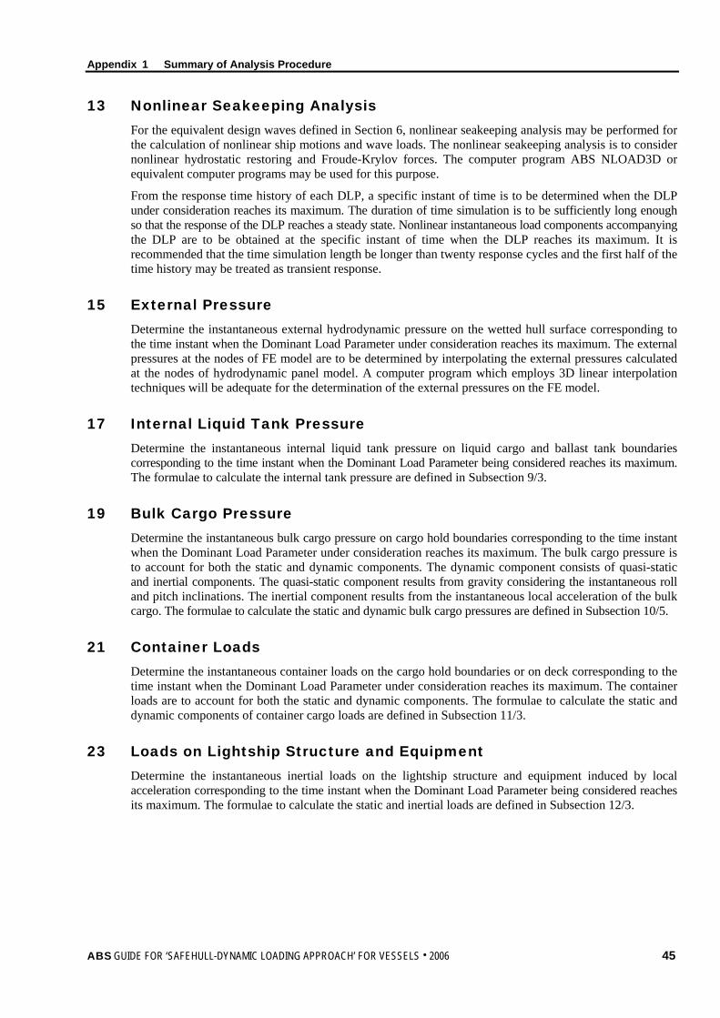
Appendix 1 Summary of Analysis Procedure
13 Nonlinear Seakeeping Analysis For the equivalent design waves defined in Section 6, nonlinear seakeeping analysis may be performed for the calculation of nonlinear ship motions and wave loads. The nonlinear seakeeping analysis is to consider nonlinear hydrostatic restoring and Froude-Krylov forces. The computer program ABS NLOAD3D or equivalent computer programs may be used for this purpose.
From the response time history of each DLP, a specific instant of time is to be determined when the DLP under consideration reaches its maximum. The duration of time simulation is to be sufficiently long enough so that the response of the DLP reaches a steady state. Nonlinear instantaneous load components accompanying the DLP are to be obtained at the specific instant of time when the DLP reaches its maximum. It is recommended that the time simulation length be longer than twenty response cycles and the first half of the time history may be treated as transient response.
15 External Pressure Determine the instantaneous external hydrodynamic pressure on the wetted hull surface corresponding to the time instant when the Dominant Load Parameter under consideration reaches its maximum. The external pressures at the nodes of FE model are to be determined by interpolating the external pressures calculated at the nodes of hydrodynamic panel model. A computer program which employs 3D linear interpolation techniques will be adequate for the determination of the external pressures on the FE model.
17 Internal Liquid Tank Pressure Determine the instantaneous internal liquid tank pressure on liquid cargo and ballast tank boundaries corresponding to the time instant when the Dominant Load Parameter being considered reaches its maximum. The formulae to calculate the internal tank pressure are defined in Subsection 9/3.
19 Bulk Cargo Pressure Determine the instantaneous bulk cargo pressure on cargo hold boundaries corresponding to the time instant when the Dominant Load Parameter under consideration reaches its maximum. The bulk cargo pressure is to account for both the static and dynamic components. The dynamic component consists of quasi-static and inertial components. The quasi-static component results from gravity considering the instantaneous roll and pitch inclinations. The inertial component results from the instantaneous local acceleration of the bulk cargo. The formulae to calculate the static and dynamic bulk cargo pressures are defined in Subsection 10/5.
21 Container Loads Determine the instantaneous container loads on the cargo hold boundaries or on deck corresponding to the time instant when the Dominant Load Parameter under consideration reaches its maximum. The container loads are to account for both the static and dynamic components. The formulae to calculate the static and dynamic components of container cargo loads are defined in Subsection 11/3.
23 Loads on Lightship Structure and Equipment Determine the instantaneous inertial loads on the lightship structure and equipment induced by local acceleration corresponding to the time instant when the Dominant Load Parameter being considered reaches its maximum. The formulae to calculate the static and inertial loads are defined in Subsection 12/3.
ABS GUIDE FOR ‘SAFEHULL-DYNAMIC LOADING APPROACH’ FOR VESSELS . 2006 45
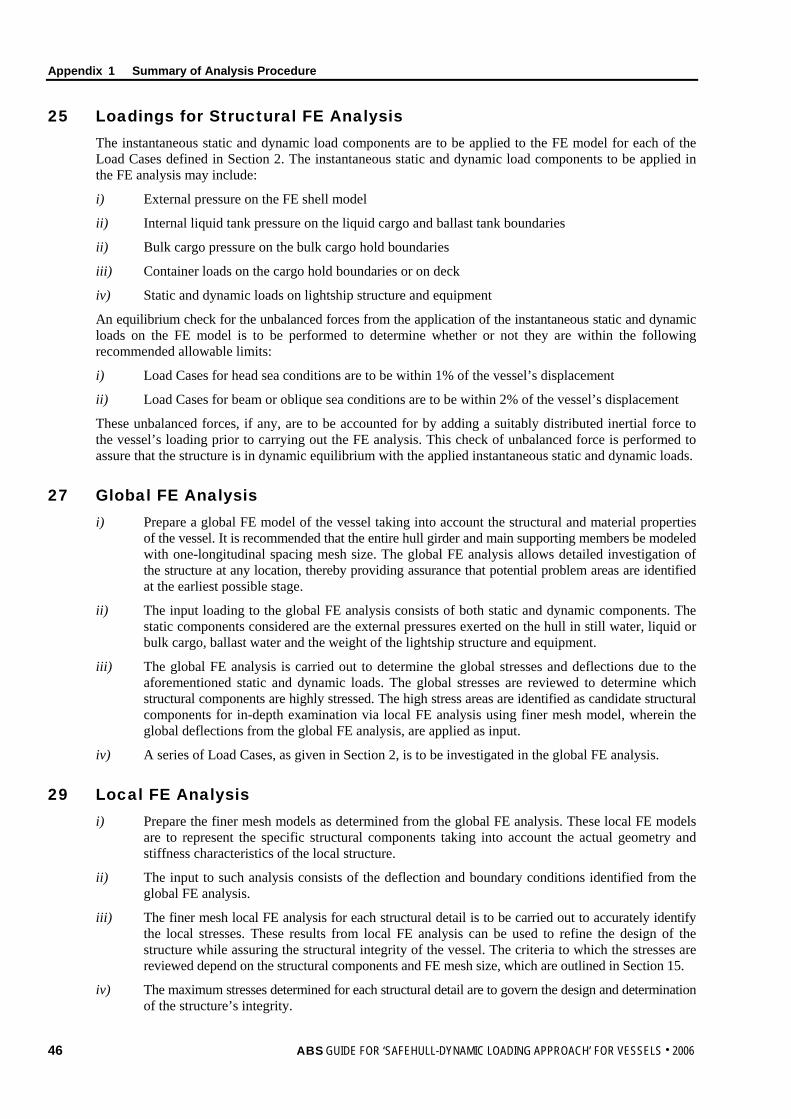
Appendix 1 Summary of Analysis Procedure 25 Loadings for Structural FE Analysis
The instantaneous static and dynamic load components are to be applied to the FE model for each of the Load Cases defined in Section 2. The instantaneous static and dynamic load components to be applied in the FE analysis may include:
i) External pressure on the FE shell model
ii) Internal liquid tank pressure on the liquid cargo and ballast tank boundaries
ii) Bulk cargo pressure on the bulk cargo hold boundaries
iii) Container loads on the cargo hold boundaries or on deck
iv) Static and dynamic loads on lightship structure and equipment
An equilibrium check for the unbalanced forces from the application of the instantaneous static and dynamic loads on the FE model is to be performed to determine whether or not they are within the following recommended allowable limits:
i) Load Cases for head sea conditions are to be within 1% of the vessel’s displacement
ii) Load Cases for beam or oblique sea conditions are to be within 2% of the vessel’s displacement
These unbalanced forces, if any, are to be accounted for by adding a suitably distributed inertial force to the vessel’s loading prior to carrying out the FE analysis. This check of unbalanced force is performed to assure that the structure is in dynamic equilibrium with the applied instantaneous static and dynamic loads.
27 Global FE Analysis i) Prepare a global FE model of the vessel taking into account the structural and material properties
of the vessel. It is recommended that the entire hull girder and main supporting members be modeled with one-longitudinal spacing mesh size. The global FE analysis allows detailed investigation of the structure at any location, thereby providing assurance that potential problem areas are identified at the earliest possible stage.
ii) The input loading to the global FE analysis consists of both static and dynamic components. The static components considered are the external pressures exerted on the hull in still water, liquid or bulk cargo, ballast water and the weight of the lightship structure and equipment.
iii) The global FE analysis is carried out to determine the global stresses and deflections due to the aforementioned static and dynamic loads. The global stresses are reviewed to determine which structural components are highly stressed. The high stress areas are identified as candidate structural components for in-depth examination via local FE analysis using finer mesh model, wherein the global deflections from the global FE analysis, are applied as input.
iv) A series of Load Cases, as given in Section 2, is to be investigated in the global FE analysis.
29 Local FE Analysis i) Prepare the finer mesh models as determined from the global FE analysis. These local FE models
are to represent the specific structural components taking into account the actual geometry and stiffness characteristics of the local structure.
ii) The input to such analysis consists of the deflection and boundary conditions identified from the global FE analysis.
iii) The finer mesh local FE analysis for each structural detail is to be carried out to accurately identify the local stresses. These results from local FE analysis can be used to refine the design of the structure while assuring the structural integrity of the vessel. The criteria to which the stresses are reviewed depend on the structural components and FE mesh size, which are outlined in Section 15.
iv) The maximum stresses determined for each structural detail are to govern the design and determination of the structure’s integrity.
46 ABS GUIDE FOR ‘SAFEHULL-DYNAMIC LOADING APPROACH’ FOR VESSELS . 2006

Appendix 1 Summary of Analysis Procedure
31 Closing Comments The primary intent of this Guide is to provide the necessary steps needed to generate the dynamic loads to be used in the structural FE analysis for the strength assessment of the vessels. The analysis procedure for Dynamic Loading Approach of the vessels described above outlines the “state-of-the-art” methods presently employed by ABS. As research in hydrodynamics identifies more advanced methods of analysis and as experience with newer designs for ships increases, modification of this procedure may be issued.
ABS GUIDE FOR ‘SAFEHULL-DYNAMIC LOADING APPROACH’ FOR VESSELS . 2006 47
A p p e n d i x 2 : B u c k l i n g a n d U l t i m a t e S t r e n g t h C r i t e r i a
A P P E N D I X 2 Buckling and Ultimate Strength Criteria
1 General
1.1 Approach The strength criteria given here correspond to either serviceability (buckling) state limit or ultimate state limit for structural members and panels, according to the intended functions and buckling resistance capability of the structure. For plate panels between stiffeners of decks, shell or plane bulkhead, buckling in the elastic range is acceptable, provided that the ultimate strength of the structure satisfies the specified design limits. The critical buckling stresses and ultimate strength of structural elements and members may be determined based on either well documented experimental data or a calibrated analytical approach. When a detailed analysis is not available, the equations given in Appendix 5C-5-A2 of the Steel Vessel Rules may be used to assess the buckling strength.
1.3 Buckling Control Concepts The strength criteria given in Section are based on the following assumptions and limitations with respect to buckling control in the design.
i) The buckling strength of longitudinals and stiffeners is generally greater than that of the plate panels being supported by the stiffeners.
ii) All of the longitudinals and stiffeners are designed to have moments of inertia with the associated effective plating not less than io, given in 5C-5-A2/11.1 of the Steel Vessel Rules.
iii) The main supporting members, including transverses, girders and floors with the effective associated plating, are to have the moment of inertia not less than is given in 5C-5-A2/11.5 of the Steel Vessel Rules.
iv) Face plates and flanges of girders, longitudinals and stiffeners are proportioned such that local instability is prevented (5C-5-A2/11.7 of the Steel Vessel Rules).
v) Webs of longitudinals and stiffeners are proportioned such that local instability is prevented (5C-5-A2/11.9 of the Steel Vessel Rules).
vi) Webs of girders, floors and transverses are designed with proper proportions and stiffening systems to prevent local instability. Critical buckling stresses of the webs may be calculated from equations given in 5C-5-A2/3 of the Steel Vessel Rules.
For structures which do not satisfy these assumptions, a detailed analysis of buckling strength using an acceptable method is to be submitted for review.
3 Plate Panels
3.1 Buckling State Limit (1 July 2005) The buckling state limit for plate panels between stiffeners is defined by the following equation:
(fL /fcL)2 + (fT /fcT)2 + (fLT /fcLT)2 ≤ 1.0
where
fL = calculated total compressive stress in the longitudinal direction for the plate, in N/cm2 (kgf/cm2, lbf/in2), induced by bending and torsion of the hull girder and large stiffened panels between bulkheads
48 ABS GUIDE FOR ‘SAFEHULL-DYNAMIC LOADING APPROACH’ FOR VESSELS . 2006

Appendix 2 Buckling and Ultimate Strength Criteria
fT = calculated total compressive stress in the transverse/vertical direction, in N/cm2 (kgf/cm2, lbf/in2)
fLT = calculated total shear stresses in the horizontal/vertical plane, in N/cm2 (kgf/cm2, lbf/in2)
fcL, fcT and fcLT are the critical buckling stresses corresponding to uniaxial compression in the longitudinal, transverse/vertical direction and edge shear, respectively, in N/cm2 (kgf/cm2, lbf/in2), and may be determined from the equations given in Appendix 5C-5-A2 of the Steel Vessel Rules.
3.3 Effective Width When the buckling state limit specified in A2/3.1 is not satisfied, the effective width bwL or bwT of the plating given below is to be used instead of the full width between longitudinals, s, for verifying the ultimate strength as specified in A2/3.5 below. When the buckling state limit in A2/3.1 is satisfied, the full width between longitudinals, s, may be used as the effective width bwL for verifying the ultimate strength of longitudinals and stiffeners specified in Subsection A2/5.
3.3.1 For Long Plate (compression on the short edges) bwL /s = Ce
where
Ce = 2.25/β − 1.25/β 2 for β > 1.25
= 1.0 for β ≤ 1.25
β = (fy /E)1/2s/tn
fy = specified minimum yield point of the material, in N/cm2 (kgf/cm2, lbf/in2)
s = stiffeners spacing, in mm (in.)
tn = net plate thickness, in mm (in.)
E = Young’s modulus for steel, 2.06 × 10⁷ N/cm2 (2.1 × 10⁶ kgf/cm2, 30 × 106 lbf/in2)
3.3.2 For Wide Plate (compression on the long edges) bwT / = Ces/ + 0.115 (1 − s/) (1+ 1/β 2)2 ≤ 1.0
where
= spacing of transverses/girders
Ce and s are as defined in A2/3.3.1.
3.5 Ultimate Strength (1 July 2005) The ultimate strength of a plate panel between stiffeners is to satisfy all of the following equations:
(fL /fuL)2 + (fLT /fuLT)2 ≤ Sm;
(fT /fuT)2 + (fLT /fuLT)2 ≤ Sm;
(fL /fuL)2 + (fT /fuT)2 − η(fL /fuL)(fT /fuT) + (fLT /fuLT)2 ≤ Sm
where
η = (1/2)(3 − β) ≥ 0
Sm = strength reduction factor for plating under consideration
= 1.0 for ordinary mild steel
= 0.95 for Grade H32 steel
= 0.908 for Grade H36 steel
= 0.875 for Grade H40 steel
ABS GUIDE FOR ‘SAFEHULL-DYNAMIC LOADING APPROACH’ FOR VESSELS . 2006 49
Appendix 2 Buckling and Ultimate Strength Criteria
fL, fT and fLT are as defined in A2/3.1.
β is as defined in A2/3.3.
fuL, fuT and fuLT are the ultimate strengths with respect to uniaxial compression and edge shear, respectively, and may be obtained from the following equations and do not need to be taken less than the corresponding critical buckling stresses specified in A2/3.1:
fuL = fy bwL /s ≥ fcL, fuT = fy bwT / ≥ fcT for plating longitudinally stiffened
fuL = fy bwT / ≥ fcL, fuT = fy bwL /s ≥ fcT for plating transversely stiffened
fuLT = fcLT + 0.5(fy − 1.73fcLT)/(1 + α + α2)1/2 ≥ fcLT
where
α = /s
fy, bwL, bwT, s, , fcL, fcT and fcLT as defined above.
When assessing the ultimate strength of plate panels between stiffeners, special attention is to be paid to the longitudinal bulkhead plating in the regions of high hull girder shear forces, and the bottom and inner bottom plating in the mid region of cargo holds subject to bi-axial compression.
5 Longitudinals and Stiffeners
5.1 Beam-Column Buckling State Limits and Ultimate Strength (2002) The buckling state limit for longitudinals and stiffeners are considered as the ultimate state limit for these members and, in combination with the effective plating, are to be determined as follows:
fa/(fca Ae /A) + m fb/fy ≤ Sm
where
fa = nominal calculated compressive stress
= P/A N/cm2 (kgf/cm2, lbf/in2)
P = total compressive load, N (kgf, lbf)
fca = critical buckling stress, as given in 5C-5-A2/5.1 of the Steel Vessel Rules, in N/cm2 (kgf/cm2, lbf/in2)
A = total net sectional area, in cm2 (in2)
= As + stn
As = net sectional area of the longitudinal, excluding the associated plating, in cm2 (in2)
Ae = effective net sectional area, in cm2 (in2)
= As + bwL tn
E = Young’s modulus for steel, 2.06 × 10⁷ N/cm2 (2.1 × 10⁶ kgf/cm2, 30 × 106 lbf/in2)
fy = minimum specified yield point of the longitudinal or stiffener under consideration, N/cm2 (kgf/cm2, lbf/in2)
fb = effective bending stress, N/cm2 (kgf/cm2, lbf/in2)
= M/SMe
M = maximum total bending moment induced by lateral loads
= Cm ps2/12 N-cm (kgf-cm, lbf-in)
50 ABS GUIDE FOR ‘SAFEHULL-DYNAMIC LOADING APPROACH’ FOR VESSELS . 2006
Appendix 2 Buckling and Ultimate Strength Criteria
Cm = moment adjustment coefficient and may be taken as 0.75
p = lateral pressure for the region considered, in N/cm2 (kgf/cm2, lbf/in2)
s = spacing of the longitudinals, cm (in.)
SMe = effective net section modulus of the longitudinal at flange, including the effective plating be, in cm3 (in3).
be = effective breadth as specified in 5C-5-4/Figure 7, line b of the Steel Vessel Rules.
m = amplification factor
= 1/[1 − fa/(π2E (r/)2] ≥ 1.0
tn and bWL are as defined in A2/3.3.1
Sm is as defined in A2/3.5
r and are as defined in 5C-5-A2/5.1 of the Steel Vessel Rules.
5.3 Torsional-Flexural Buckling State Limit (2002) In general, the torsional-flexural buckling state limit of longitudinals and stiffeners is to satisfy the ultimate state limits given below:
fa/( fct Ae/A) ≤ Sm
where
fa = nominal calculated compressive stress, in N/cm2 (kgf/cm2, lbf/in2), as defined in A2/5.1
fct = critical torsional-flexural buckling stress, in N/cm2 (kgf/cm2, lbf/in2), and may be determined by equations given in 5C-5-A2/5.5 of the Steel Vessel Rules.
Ae and A are as defined in A2/5.1 and Sm is as defined in A2/3.5.
7 Stiffened Panels
7.1 Large Stiffened Panels Between Bulkheads For a vessel under the assumptions made in A2/1.3 with respect to the buckling control concepts, the large stiffened panels of the double bottom and double side structures between transverse bulkheads should automatically satisfy the design limits, provided that each individual plate panel and longitudinally and uniaxially stiffened panel satisfy the specified ultimate state limits. Assessments of the buckling state limits are to be performed for large stiffened panels of the single side shell and plane transverse bulkheads. In this regard, the buckling strength is to satisfy the following condition for uniaxially or orthogonally stiffened panels.
(fL /fcL)2 + (fT /fcT)2 ≤ Sm
where
fL , fT = calculated average compressive stresses in the longitudinal and transverse/vertical directions, respectively, in N/cm2 (kgf/cm2, lbf/in2).
fcL, fcT = critical buckling stresses for uniaxial compression in the longitudinal and transverse direction, respectively, and may be determined in accordance with 5C-5-A2/7 of the Steel Vessel Rules, in N/cm2 (kgf/cm2, lbf/in2)
Sm = strength reduction factor, as defined in A2/3.5
7.3 Uniaxially Stiffened Panels between Transverses and Girders The buckling strength of uniaxially stiffened panels between deep transverses and girders is also to be examined in accordance with the specifications given in A2/7.1.
ABS GUIDE FOR ‘SAFEHULL-DYNAMIC LOADING APPROACH’ FOR VESSELS . 2006 51
Appendix 2 Buckling and Ultimate Strength Criteria
9 Deep Girders and Webs
9.1 Buckling Criteria In general, the stiffness of the web stiffeners along the depth of the web plating is to be in compliance with the requirements 5C-5-A2/11.3 of the Steel Vessel Rules. Web stiffeners which are oriented parallel to and near the face plate and thus subject to axial compression are also to satisfy the limits specified in Subsection A2/5, considering the combined effect of the compressive and bending stresses in the web. In this case, the unsupported span of these parallel stiffeners may be taken between tripping brackets, as applicable.
The buckling strength of the web plate between stiffeners and flange/face plate is to satisfy the limits specified below:
9.1.1 Web Plate (1 October 2015) (fL /fcL)2 + (fb /fcb)
2 + (fLT /fcLT)2 ≤ Sm
where
fL = calculated uniform compressive stress along the length of the girder, in N/cm2 (kgf/cm2, lbf/in2).
fb = calculated ideal bending stress, in N/cm2 (kgf/cm2, lbf/in2).
fLT = calculated total shear stress, including hull girder and local loads where applicable, in N/cm2 (kgf/cm2, lbf/in2).
fL, fb and fLT are to be calculated for the panel in question under each load case. fL, fb and fLT may be calculated by the relative displacement of four corner nodes of the panel. Care is to be taken where one corner of the panel is located in a high stress concentration area; because stresses calculated by the displacement method tend to be conservative. fL, fb and fLT may also be directly calculated from the component stresses of the elements in the panel, provided sufficient number of elements exists to represent stress distributions in the panel. fcL, fcb and fcLT are critical buckling stresses with respect to uniform compression, ideal bending and shear, respectively, and may be determined in accordance with 5C-5-A2 of the Steel Vessel Rules.
Sm is as defined in A2/3.5.
In the determination of fcL and fcLT, the effects of openings are to be appropriately considered.
9.1.2 Face Plate and Flange The breadth to thickness ratio of face plate and flange is to satisfy the limits given in 5C-5-A2/11.7 of the Steel Vessel Rules.
9.1.3 Large Brackets and Sloping Webs The buckling strength is to satisfy the limits specified in A2/9.1.2 for web plate.
9.3 Tripping Tripping brackets are to be provided in accordance with 5C-5-A2/9.5 of the Steel Vessel Rules.
52 ABS GUIDE FOR ‘SAFEHULL-DYNAMIC LOADING APPROACH’ FOR VESSELS . 2006
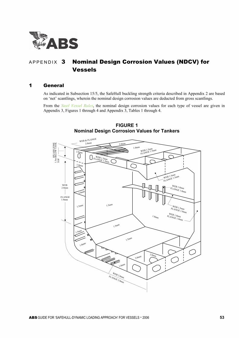
ABS GUIDE FOR ‘SAFEHULL-DYNAMIC LOADING APPROACH’ FOR VESSELS . 2006 53
A p p e n d i x 3 : N o m i n a l D e s i g n C o r r o s i o n V a l u e s ( N D C V ) f o r V e s s e l s
A P P E N D I X 3 Nominal Design Corrosion Values (NDCV) for Vessels
1 General As indicated in Subsection 15/5, the SafeHull buckling strength criteria described in Appendix 2 are based on ‘net’ scantlings, wherein the nominal design corrosion values are deducted from gross scantlings.
From the Steel Vessel Rules, the nominal design corrosion values for each type of vessel are given in Appendix 3, Figures 1 through 4 and Appendix 3, Tables 1 through 4.
FIGURE 1 Nominal Design Corrosion Values for Tankers
WEB & FLANGE
2.0mm2.0mm
1.0mm
WEB 1.5mm
FLANGE 1.5mm
WEB 1.5mm
FLANGE 1.5mm
WEB 1.0mmFLANGE 1.0mm
WEB 1.5mmFLANGE 1.0mmWEB 1.0mmFLANGE 1.0mm
1.0mm
1.5mm
1.5mm
1.5mm
WEB 1.5mmFLANGE 1.5mm
2.0mm
1.0mm
2.0mm
1.5mm
1.0mm
1.5mm
1.0mm
2.0mm2.0mm
2.0mm
1.0mmFLANGE
WEB 2.0mmFLANGE 2.0mm
1.5m
BE
LO
W T
AN
KT
OP
SPL
ASH
ZO
NE
WEB
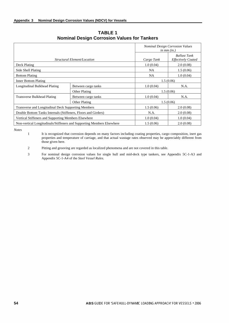
Appendix 3 Nominal Design Corrosion Values (NDCV) for Vessels
TABLE 1 Nominal Design Corrosion Values for Tankers
Nominal Design Corrosion Values in mm (in.)
Structural Element/Location Cargo Tank Ballast Tank
Effectively Coated Deck Plating 1.0 (0.04) 2.0 (0.08) Side Shell Plating NA 1.5 (0.06) Bottom Plating NA 1.0 (0.04) Inner Bottom Plating 1.5 (0.06) Longitudinal Bulkhead Plating Between cargo tanks 1.0 (0.04) N.A. Other Plating 1.5 (0.06) Transverse Bulkhead Plating Between cargo tanks 1.0 (0.04) N.A. Other Plating 1.5 (0.06) Transverse and Longitudinal Deck Supporting Members 1.5 (0.06) 2.0 (0.08) Double Bottom Tanks Internals (Stiffeners, Floors and Girders) N.A. 2.0 (0.08) Vertical Stiffeners and Supporting Members Elsewhere 1.0 (0.04) 1.0 (0.04) Non-vertical Longitudinals/Stiffeners and Supporting Members Elsewhere 1.5 (0.06) 2.0 (0.08)
Notes 1 It is recognized that corrosion depends on many factors including coating properties, cargo composition, inert gas
properties and temperature of carriage, and that actual wastage rates observed may be appreciably different from those given here.
2 Pitting and grooving are regarded as localized phenomena and are not covered in this table.
3 For nominal design corrosion values for single hull and mid-deck type tankers, see Appendix 5C-1-A3 and Appendix 5C-1-A4 of the Steel Vessel Rules.
54 ABS GUIDE FOR ‘SAFEHULL-DYNAMIC LOADING APPROACH’ FOR VESSELS . 2006
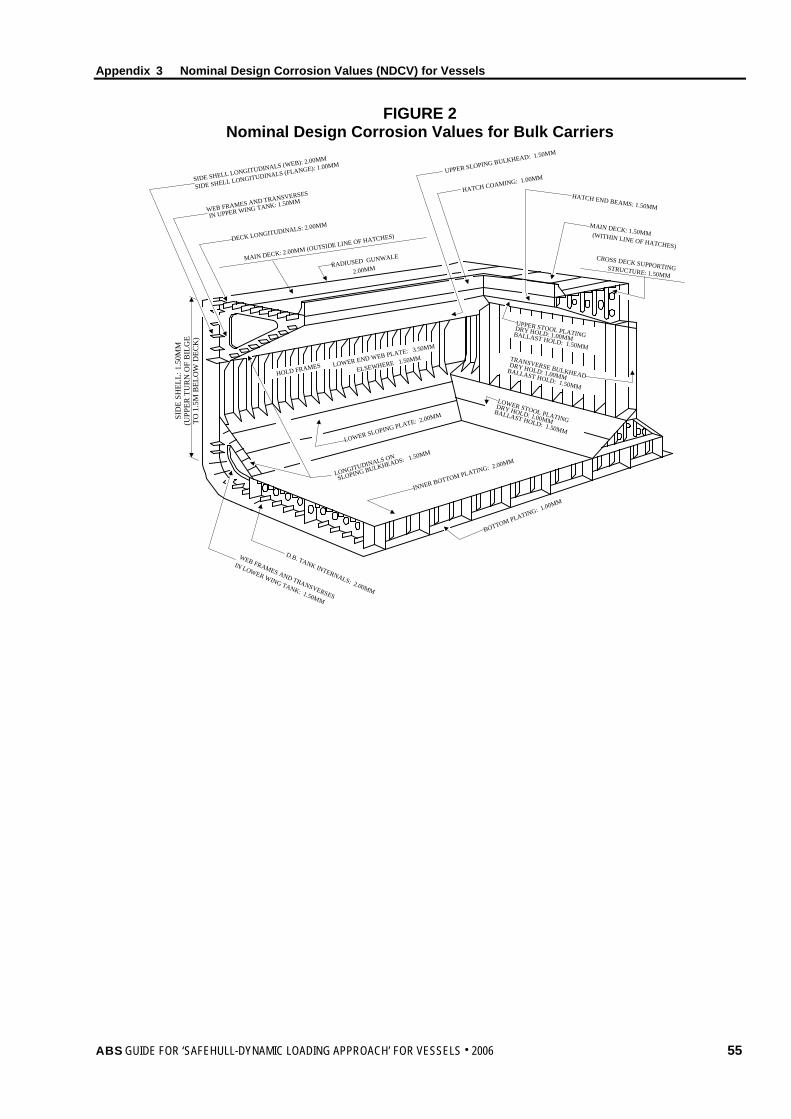
Appendix 3 Nominal Design Corrosion Values (NDCV) for Vessels
FIGURE 2 Nominal Design Corrosion Values for Bulk Carriers
SIDE SHELL LONGITUDINALS (WEB): 2.00MM
SIDE SHELL LONGITUDINALS (FLANGE): 1.00MM
IN UPPER WING TANK: 1.50MMWEB FRAMES AND TRANSVERSES
DECK LONGITUDINALS: 2.00MM
MAIN DECK: 2.00MM (OUTSIDE LINE OF HATCHES)
RADIUSED GUNWALE
2.00MM
HATCH END BEAMS: 1.50MM
MAIN DECK: 1.50MM(WITHIN LINE OF HATCHES)
CROSS DECK SUPPORTINGSTRUCTURE: 1.50MM
UPPER SLOPING BULKHEAD: 1.50MM
HATCH COAMING: 1.00MM
LOWER END WEB PLATE: 3.50MM
ELSEWHERE 1.50MM
HOLD FRAMES
UPPER STOOL PLATINGDRY HOLD: 1.00MMBALLAST HOLD: 1.50MM
TRANSVERSE BULKHEADDRY HOLD: 1.00MM
BALLAST HOLD: 1.50MM
LOWER STOOL PLATING
DRY HOLD: 1.00MMBALLAST HOLD: 1.50MM
D.B. TANK INTERNALS: 2.00MM
WEB FRAMES AND TRANSVERSES
IN LOWER WING TANK: 1.50MM
LOWER SLOPING PLATE: 2.00MM
LONGITUDINALS ON
SLOPING BULKHEADS: 1.50MM
INNER BOTTOM PLATING: 2.00MM
BOTTOM PLATING: 1.00MM
SID
E SH
ELL:
1.5
0MM
(UPP
ER T
UR
N O
F B
ILG
ETO
1.5
M B
ELO
W D
ECK
)
ABS GUIDE FOR ‘SAFEHULL-DYNAMIC LOADING APPROACH’ FOR VESSELS . 2006 55
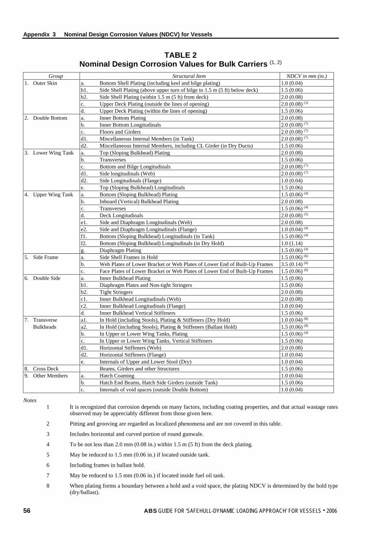
Appendix 3 Nominal Design Corrosion Values (NDCV) for Vessels
TABLE 2 Nominal Design Corrosion Values for Bulk Carriers (1, 2)
Group Structural Item NDCV in mm (in.) 1. Outer Skin a. Bottom Shell Plating (including keel and bilge plating) 1.0 (0.04) b1. Side Shell Plating (above upper turn of bilge to 1.5 m (5 ft) below deck) 1.5 (0.06) b2. Side Shell Plating (within 1.5 m (5 ft) from deck) 2.0 (0.08) c. Upper Deck Plating (outside the lines of opening) 2.0 (0.08) (3) d. Upper Deck Plating (within the lines of opening) 1.5 (0.06) 2. Double Bottom a. Inner Bottom Plating 2.0 (0.08) b. Inner Bottom Longitudinals 2.0 (0.08) (7) c. Floors and Girders 2.0 (0.08) (7) d1. Miscellaneous Internal Members (in Tank) 2.0 (0.08) (7) d2. Miscellaneous Internal Members, including CL Girder (in Dry Ducts) 1.5 (0.06) 3. Lower Wing Tank a. Top (Sloping Bulkhead) Plating 2.0 (0.08) b. Transverses 1.5 (0.06) c. Bottom and Bilge Longitudinals 2.0 (0.08) (7) d1. Side longitudinals (Web) 2.0 (0.08) (7) d2. Side Longitudinals (Flange) 1.0 (0.04) e. Top (Sloping Bulkhead) Longitudinals 1.5 (0.06) 4. Upper Wing Tank a. Bottom (Sloping Bulkhead) Plating 1.5 (0.06) (4) b. Inboard (Vertical) Bulkhead Plating 2.0 (0.08) c. Transverses 1.5 (0.06) (4) d. Deck Longitudinals 2.0 (0.08) (5) e1. Side and Diaphragm Longitudinals (Web) 2.0 (0.08) e2. Side and Diaphragm Longitudinals (Flange) 1.0 (0.04) (4) f1. Bottom (Sloping Bulkhead) Longitudinals (in Tank) 1.5 (0.06) (4) f2. Bottom (Sloping Bulkhead) Longitudinals (in Dry Hold) 1.0 (1.14) g. Diaphragm Plating 1.5 (0.06) (4) 5. Side Frame a. Side Shell Frames in Hold 1.5 (0.06) (6) b. Web Plates of Lower Bracket or Web Plates of Lower End of Built-Up Frames 3.5 (0.14) (6) c. Face Plates of Lower Bracket or Web Plates of Lower End of Built-Up Frames 1.5 (0.06) (6) 6. Double Side a. Inner Bulkhead Plating 1.5 (0.06) b1. Diaphragm Plates and Non-tight Stringers 1.5 (0.06) b2. Tight Stringers 2.0 (0.08) c1. Inner Bulkhead Longitudinals (Web) 2.0 (0.08) c2. Inner Bulkhead Longitudinals (Flange) 1.0 (0.04) d. Inner Bulkhead Vertical Stiffeners 1.5 (0.06) 7. Transverse a1. In Hold (including Stools), Plating & Stiffeners (Dry Hold) 1.0 (0.04) (8) Bulkheads a2. In Hold (including Stools), Plating & Stiffeners (Ballast Hold) 1.5 (0.06) (8) b. In Upper or Lower Wing Tanks, Plating 1.5 (0.06) (4) c. In Upper or Lower Wing Tanks, Vertical Stiffeners 1.5 (0.06) d1. Horizontal Stiffeners (Web) 2.0 (0.08) d2. Horizontal Stiffeners (Flange) 1.0 (0.04) e. Internals of Upper and Lower Stool (Dry) 1.0 (0.04) 8. Cross Deck Beams, Girders and other Structures 1.5 (0.06) 9. Other Members a. Hatch Coaming 1.0 (0.04) b. Hatch End Beams, Hatch Side Girders (outside Tank) 1.5 (0.06) c. Internals of void spaces (outside Double Bottom) 1.0 (0.04)
Notes 1 It is recognized that corrosion depends on many factors, including coating properties, and that actual wastage rates
observed may be appreciably different from those given here.
2 Pitting and grooving are regarded as localized phenomena and are not covered in this table.
3 Includes horizontal and curved portion of round gunwale.
4 To be not less than 2.0 mm (0.08 in.) within 1.5 m (5 ft) from the deck plating.
5 May be reduced to 1.5 mm (0.06 in.) if located outside tank.
6 Including frames in ballast hold.
7 May be reduced to 1.5 mm (0.06 in.) if located inside fuel oil tank.
8 When plating forms a boundary between a hold and a void space, the plating NDCV is determined by the hold type (dry/ballast).
56 ABS GUIDE FOR ‘SAFEHULL-DYNAMIC LOADING APPROACH’ FOR VESSELS . 2006
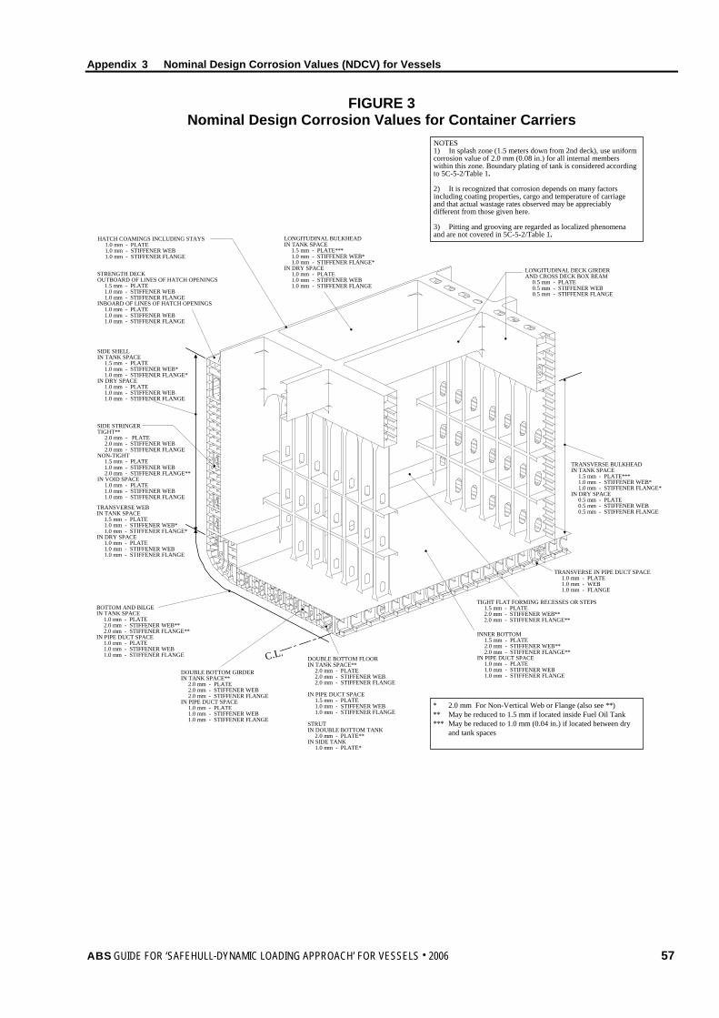
Appendix 3 Nominal Design Corrosion Values (NDCV) for Vessels
FIGURE 3 Nominal Design Corrosion Values for Container Carriers
LONGITUDINAL DECK GIRDERAND CROSS DECK BOX BEAM
0.5 mm - PLATE0.5 mm - STIFFENER WEB0.5 mm - STIFFENER FLANGE
TRANSVERSE BULKHEADIN TANK SPACE
1.5 mm - PLATE***1.0 mm - STIFFENER WEB*1.0 mm - STIFFENER FLANGE*
IN DRY SPACE0.5 mm - PLATE0.5 mm - STIFFENER WEB0.5 mm - STIFFENER FLANGE
TRANSVERSE IN PIPE DUCT SPACE1.0 mm - PLATE1.0 mm - WEB1.0 mm - FLANGE
TIGHT FLAT FORMING RECESSES OR STEPS1.5 mm - PLATE2.0 mm - STIFFENER WEB**2.0 mm - STIFFENER FLANGE**
INNER BOTTOM1.5 mm - PLATE2.0 mm - STIFFENER WEB**2.0 mm - STIFFENER FLANGE**
IN PIPE DUCT SPACE1.0 mm - PLATE1.0 mm - STIFFENER WEB1.0 mm - STIFFENER FLANGE
DOUBLE BOTTOM FLOORIN TANK SPACE**
2.0 mm - PLATE2.0 mm - STIFFENER WEB2.0 mm - STIFFENER FLANGE
IN PIPE DUCT SPACE1.5 mm - PLATE1.0 mm - STIFFENER WEB1.0 mm - STIFFENER FLANGE
STRUTIN DOUBLE BOTTOM TANK
2.0 mm - PLATE**IN SIDE TANK
1.0 mm - PLATE*
* 2.0 mm For Non-Vertical Web or Flange (also see **)** May be reduced to 1.5 mm if located inside Fuel Oil Tank*** May be reduced to 1.0 mm (0.04 in.) if located between dry
and tank spaces
DOUBLE BOTTOM GIRDERIN TANK SPACE**
2.0 mm - PLATE2.0 mm - STIFFENER WEB2.0 mm - STIFFENER FLANGE
IN PIPE DUCT SPACE1.0 mm - PLATE1.0 mm - STIFFENER WEB1.0 mm - STIFFENER FLANGE
HATCH COAMINGS INCLUDING STAYS1.0 mm - PLATE1.0 mm - STIFFENER WEB1.0 mm - STIFFENER FLANGE
STRENGTH DECKOUTBOARD OF LINES OF HATCH OPENINGS
1.5 mm - PLATE1.0 mm - STIFFENER WEB1.0 mm - STIFFENER FLANGE
INBOARD OF LINES OF HATCH OPENINGS1.0 mm - PLATE1.0 mm - STIFFENER WEB1.0 mm - STIFFENER FLANGE
SIDE SHELLIN TANK SPACE
1.5 mm - PLATE1.0 mm - STIFFENER WEB*1.0 mm - STIFFENER FLANGE*
IN DRY SPACE1.0 mm - PLATE1.0 mm - STIFFENER WEB1.0 mm - STIFFENER FLANGE
SIDE STRINGERTIGHT**
2.0 mm - PLATE2.0 mm - STIFFENER WEB2.0 mm - STIFFENER FLANGE
NON-TIGHT1.5 mm - PLATE1.0 mm - STIFFENER WEB2.0 mm - STIFFENER FLANGE**
IN VOID SPACE1.0 mm - PLATE1.0 mm - STIFFENER WEB1.0 mm - STIFFENER FLANGE
TRANSVERSE WEBIN TANK SPACE
1.5 mm - PLATE1.0 mm - STIFFENER WEB*1.0 mm - STIFFENER FLANGE*
IN DRY SPACE1.0 mm - PLATE1.0 mm - STIFFENER WEB1.0 mm - STIFFENER FLANGE
BOTTOM AND BILGEIN TANK SPACE
1.0 mm - PLATE2.0 mm - STIFFENER WEB**2.0 mm - STIFFENER FLANGE**
IN PIPE DUCT SPACE1.0 mm - PLATE1.0 mm - STIFFENER WEB1.0 mm - STIFFENER FLANGE
LONGITUDINAL BULKHEADIN TANK SPACE
1.5 mm - PLATE***1.0 mm - STIFFENER WEB*1.0 mm - STIFFENER FLANGE*
IN DRY SPACE1.0 mm - PLATE1.0 mm - STIFFENER WEB1.0 mm - STIFFENER FLANGE
NOTES1) In splash zone (1.5 meters down from 2nd deck), use uniformcorrosion value of 2.0 mm (0.08 in.) for all internal memberswithin this zone. Boundary plating of tank is considered accordingto 5C-5-2/Table 1.
2) It is recognized that corrosion depends on many factorsincluding coating properties, cargo and temperature of carriageand that actual wastage rates observed may be appreciablydifferent from those given here.
3) Pitting and grooving are regarded as localized phenomenaand are not covered in 5C-5-2/Table 1.
C.L.
ABS GUIDE FOR ‘SAFEHULL-DYNAMIC LOADING APPROACH’ FOR VESSELS . 2006 57
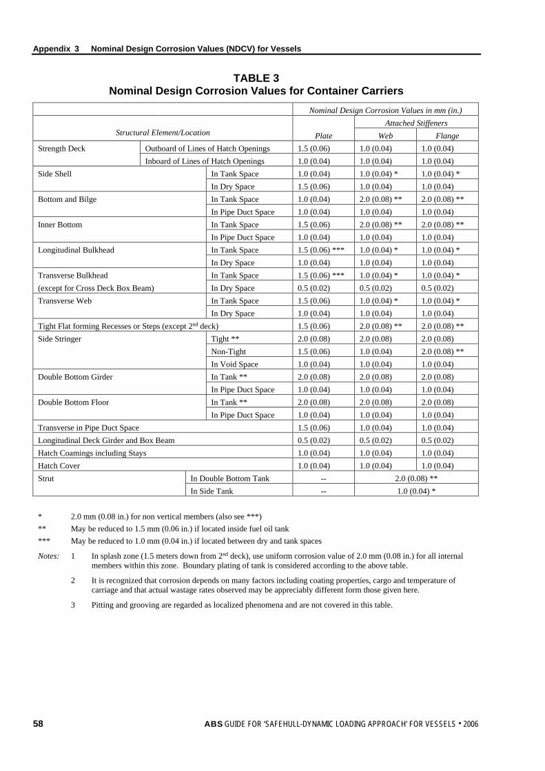
Appendix 3 Nominal Design Corrosion Values (NDCV) for Vessels
TABLE 3 Nominal Design Corrosion Values for Container Carriers
Nominal Design Corrosion Values in mm (in.)
Structural Element/Location Attached Stiffeners
Plate Web Flange Strength Deck Outboard of Lines of Hatch Openings 1.5 (0.06) 1.0 (0.04) 1.0 (0.04) Inboard of Lines of Hatch Openings 1.0 (0.04) 1.0 (0.04) 1.0 (0.04) Side Shell In Tank Space 1.0 (0.04) 1.0 (0.04) * 1.0 (0.04) * In Dry Space 1.5 (0.06) 1.0 (0.04) 1.0 (0.04) Bottom and Bilge In Tank Space 1.0 (0.04) 2.0 (0.08) ** 2.0 (0.08) ** In Pipe Duct Space 1.0 (0.04) 1.0 (0.04) 1.0 (0.04) Inner Bottom In Tank Space 1.5 (0.06) 2.0 (0.08) ** 2.0 (0.08) ** In Pipe Duct Space 1.0 (0.04) 1.0 (0.04) 1.0 (0.04) Longitudinal Bulkhead In Tank Space 1.5 (0.06) *** 1.0 (0.04) * 1.0 (0.04) * In Dry Space 1.0 (0.04) 1.0 (0.04) 1.0 (0.04) Transverse Bulkhead In Tank Space 1.5 (0.06) *** 1.0 (0.04) * 1.0 (0.04) * (except for Cross Deck Box Beam) In Dry Space 0.5 (0.02) 0.5 (0.02) 0.5 (0.02) Transverse Web In Tank Space 1.5 (0.06) 1.0 (0.04) * 1.0 (0.04) * In Dry Space 1.0 (0.04) 1.0 (0.04) 1.0 (0.04) Tight Flat forming Recesses or Steps (except 2nd deck) 1.5 (0.06) 2.0 (0.08) ** 2.0 (0.08) ** Side Stringer Tight ** 2.0 (0.08) 2.0 (0.08) 2.0 (0.08) Non-Tight 1.5 (0.06) 1.0 (0.04) 2.0 (0.08) ** In Void Space 1.0 (0.04) 1.0 (0.04) 1.0 (0.04) Double Bottom Girder In Tank ** 2.0 (0.08) 2.0 (0.08) 2.0 (0.08) In Pipe Duct Space 1.0 (0.04) 1.0 (0.04) 1.0 (0.04) Double Bottom Floor In Tank ** 2.0 (0.08) 2.0 (0.08) 2.0 (0.08) In Pipe Duct Space 1.0 (0.04) 1.0 (0.04) 1.0 (0.04) Transverse in Pipe Duct Space 1.5 (0.06) 1.0 (0.04) 1.0 (0.04) Longitudinal Deck Girder and Box Beam 0.5 (0.02) 0.5 (0.02) 0.5 (0.02) Hatch Coamings including Stays 1.0 (0.04) 1.0 (0.04) 1.0 (0.04) Hatch Cover 1.0 (0.04) 1.0 (0.04) 1.0 (0.04) Strut In Double Bottom Tank -- 2.0 (0.08) ** In Side Tank -- 1.0 (0.04) *
* 2.0 mm (0.08 in.) for non vertical members (also see ***) ** May be reduced to 1.5 mm (0.06 in.) if located inside fuel oil tank *** May be reduced to 1.0 mm (0.04 in.) if located between dry and tank spaces
Notes: 1 In splash zone (1.5 meters down from 2nd deck), use uniform corrosion value of 2.0 mm (0.08 in.) for all internal members within this zone. Boundary plating of tank is considered according to the above table.
2 It is recognized that corrosion depends on many factors including coating properties, cargo and temperature of carriage and that actual wastage rates observed may be appreciably different form those given here.
3 Pitting and grooving are regarded as localized phenomena and are not covered in this table.
58 ABS GUIDE FOR ‘SAFEHULL-DYNAMIC LOADING APPROACH’ FOR VESSELS . 2006
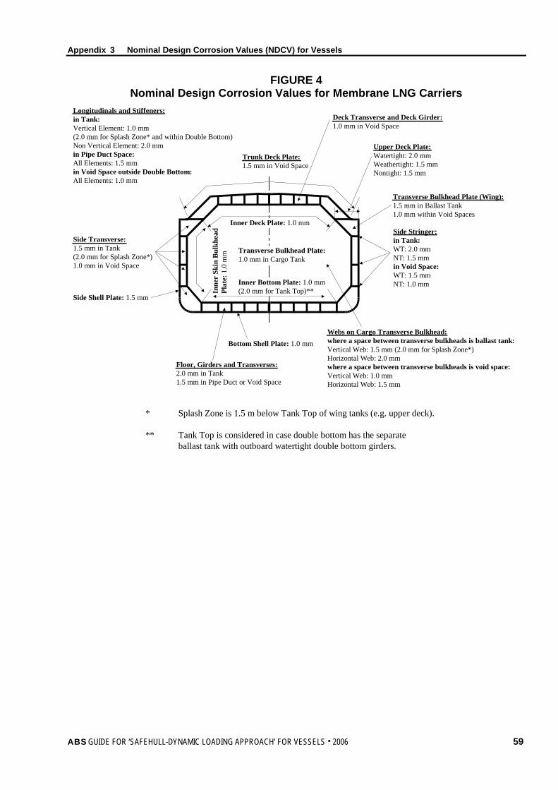
Appendix 3 Nominal Design Corrosion Values (NDCV) for Vessels
FIGURE 4 Nominal Design Corrosion Values for Membrane LNG Carriers
Trunk Deck Plate:1.5 mm in Void Space
Deck Transverse and Deck Girder:1.0 mm in Void Space
Upper Deck Plate:Watertight: 2.0 mmWeathertight: 1.5 mmNontight: 1.5 mm
Transverse Bulkhead Plate (Wing):1.5 mm in Ballast Tank1.0 mm within Void Spaces
Side Stringer:in Tank:WT: 2.0 mmNT: 1.5 mmin Void Space:WT: 1.5 mmNT: 1.0 mm
Longitudinals and Stiffeners:in Tank:Vertical Element: 1.0 mm(2.0 mm for Splash Zone* and within Double Bottom)Non Vertical Element: 2.0 mmin Pipe Duct Space:All Elements: 1.5 mmin Void Space outside Double Bottom:All Elements: 1.0 mm
Side Transverse:1.5 mm in Tank(2.0 mm for Splash Zone*)1.0 mm in Void Space
Side Shell Plate: 1.5 mm
Bottom Shell Plate: 1.0 mm
Floor, Girders and Transverses:2.0 mm in Tank1.5 mm in Pipe Duct or Void Space
Webs on Cargo Transverse Bulkhead:where a space between transverse bulkheads is ballast tank:Vertical Web: 1.5 mm (2.0 mm for Splash Zone*)Horizontal Web: 2.0 mmwhere a space between transverse bulkheads is void space:Vertical Web: 1.0 mmHorizontal Web: 1.5 mm
Inner Bottom Plate: 1.0 mm(2.0 mm for Tank Top)**
Transverse Bulkhead Plate:1.0 mm in Cargo Tank
Inner Deck Plate: 1.0 mmIn
ner
Skin
Bul
khea
dPl
ate:
1.0
mm
* Splash Zone is 1.5 m below Tank Top of wing tanks (e.g. upper deck).
** Tank Top is considered in case double bottom has the separateballast tank with outboard watertight double bottom girders.
ABS GUIDE FOR ‘SAFEHULL-DYNAMIC LOADING APPROACH’ FOR VESSELS . 2006 59
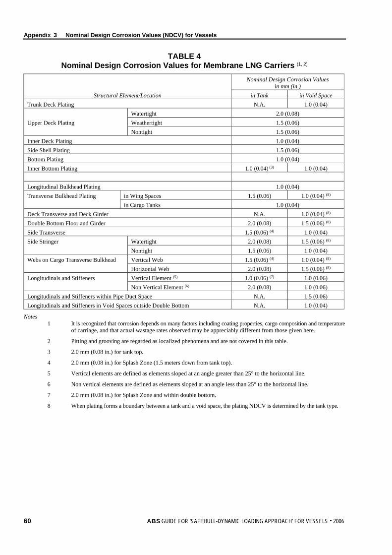
Appendix 3 Nominal Design Corrosion Values (NDCV) for Vessels
TABLE 4 Nominal Design Corrosion Values for Membrane LNG Carriers (1, 2)
Nominal Design Corrosion Values in mm (in.)
Structural Element/Location in Tank in Void Space Trunk Deck Plating N.A. 1.0 (0.04) Watertight 2.0 (0.08) Upper Deck Plating Weathertight 1.5 (0.06) Nontight 1.5 (0.06) Inner Deck Plating 1.0 (0.04) Side Shell Plating 1.5 (0.06) Bottom Plating 1.0 (0.04) Inner Bottom Plating 1.0 (0.04) (3) 1.0 (0.04) Longitudinal Bulkhead Plating 1.0 (0.04) Transverse Bulkhead Plating in Wing Spaces 1.5 (0.06) 1.0 (0.04) (8) in Cargo Tanks 1.0 (0.04) Deck Transverse and Deck Girder N.A. 1.0 (0.04) (8) Double Bottom Floor and Girder 2.0 (0.08) 1.5 (0.06) (8) Side Transverse 1.5 (0.06) (4) 1.0 (0.04) Side Stringer Watertight 2.0 (0.08) 1.5 (0.06) (8) Nontight 1.5 (0.06) 1.0 (0.04) Webs on Cargo Transverse Bulkhead Vertical Web 1.5 (0.06) (4) 1.0 (0.04) (8) Horizontal Web 2.0 (0.08) 1.5 (0.06) (8) Longitudinals and Stiffeners Vertical Element (5) 1.0 (0.06) (7) 1.0 (0.06) Non Vertical Element (6) 2.0 (0.08) 1.0 (0.06) Longitudinals and Stiffeners within Pipe Duct Space N.A. 1.5 (0.06) Longitudinals and Stiffeners in Void Spaces outside Double Bottom N.A. 1.0 (0.04)
Notes 1 It is recognized that corrosion depends on many factors including coating properties, cargo composition and temperature
of carriage, and that actual wastage rates observed may be appreciably different from those given here.
2 Pitting and grooving are regarded as localized phenomena and are not covered in this table.
3 2.0 mm (0.08 in.) for tank top.
4 2.0 mm (0.08 in.) for Splash Zone (1.5 meters down from tank top).
5 Vertical elements are defined as elements sloped at an angle greater than 25° to the horizontal line.
6 Non vertical elements are defined as elements sloped at an angle less than 25° to the horizontal line.
7 2.0 mm (0.08 in.) for Splash Zone and within double bottom.
8 When plating forms a boundary between a tank and a void space, the plating NDCV is determined by the tank type.
60 ABS GUIDE FOR ‘SAFEHULL-DYNAMIC LOADING APPROACH’ FOR VESSELS . 2006