ascet v6.0 getting started - etas · pdf file4.6.1 motion equation ... reductions a reality....

ASCET V6.0Getting Started

2

Copyright

The data in this document may not be altered or amended without specialnotification from ETAS GmbH. ETAS GmbH undertakes no further obligation inrelation to this document. The software described in it can only be used if thecustomer is in possession of a general license agreement or single license. Using and copying is only allowed in concurrence with the specifications stip-ulated in the contract.

Under no circumstances may any part of this document be copied, repro-duced, transmitted, stored in a retrieval system or translated into another lan-guage without the express written permission of ETAS GmbH.

© Copyright 2008 ETAS GmbH, Stuttgart

The names and designations used in this document are trademarks or brandsbelonging to the respective owners.

The name INTECRIO is a registered trademark of ETAS GmbH.

Document EC010010 R6.0.2 EN TN F 00K 103 222

Contents
1 Introduction . . . . . . . . . . . . . . . . . . . . . . . . . . . . . . . . . . . . . . . . . . . . . . . . . . . . . 7
1.1 System Information . . . . . . . . . . . . . . . . . . . . . . . . . . . . . . . . . . . . . . . . . . 71.2 User Information . . . . . . . . . . . . . . . . . . . . . . . . . . . . . . . . . . . . . . . . . . . . 7

1.2.1 User Profile. . . . . . . . . . . . . . . . . . . . . . . . . . . . . . . . . . . . . . . . . 71.2.2 Documentation Structure . . . . . . . . . . . . . . . . . . . . . . . . . . . . . . 81.2.3 How to Use this Manual . . . . . . . . . . . . . . . . . . . . . . . . . . . . . . . 9

1.3 Supporting Functions . . . . . . . . . . . . . . . . . . . . . . . . . . . . . . . . . . . . . . . 111.3.1 Monitor Window . . . . . . . . . . . . . . . . . . . . . . . . . . . . . . . . . . . 111.3.2 Keyboard Assignment. . . . . . . . . . . . . . . . . . . . . . . . . . . . . . . . 121.3.3 Manual and Online Help. . . . . . . . . . . . . . . . . . . . . . . . . . . . . . 12

2 Embedded Automotive Control Software Development with ASCET . . . . . . . . . . 132.1 Model-Based Design . . . . . . . . . . . . . . . . . . . . . . . . . . . . . . . . . . . . . . . . 14

2.1.1 Control Algorithm Development. . . . . . . . . . . . . . . . . . . . . . . . 152.1.2 Rapid Prototyping. . . . . . . . . . . . . . . . . . . . . . . . . . . . . . . . . . . 202.1.3 Implementation and ECU Integration of Control Algorithms . . . 222.1.4 Reuse of the Control Algorithm in Different Kinds of

Projects . . . . . . . . . . . . . . . . . . . . . . . . . . . . . . . . . . . . . . . . . . 272.1.5 Testing the Technical System Architecture in the Lab . . . . . . . . . 28

Contents 3

4

2.1.6 Testing and Honing of the Technical System Architecture inthe Vehicle . . . . . . . . . . . . . . . . . . . . . . . . . . . . . . . . . . . . . . . . 29

2.2 Using ASCET in a Production Environment . . . . . . . . . . . . . . . . . . . . . . . . 292.2.1 Model Conversion . . . . . . . . . . . . . . . . . . . . . . . . . . . . . . . . . . 30

2.3 Summary . . . . . . . . . . . . . . . . . . . . . . . . . . . . . . . . . . . . . . . . . . . . . . . . . 32

3 ASCET and AUTOSAR. . . . . . . . . . . . . . . . . . . . . . . . . . . . . . . . . . . . . . . . . . . . . 333.1 Overview . . . . . . . . . . . . . . . . . . . . . . . . . . . . . . . . . . . . . . . . . . . . . . . . . 33

3.1.1 RTA-RTE and RTA-OS . . . . . . . . . . . . . . . . . . . . . . . . . . . . . . . . 343.1.2 Creating AUTOSAR Software Components . . . . . . . . . . . . . . . . 35

3.2 What is a Runtime Environment? . . . . . . . . . . . . . . . . . . . . . . . . . . . . . . . 353.3 AUTOSAR Elements in ASCET . . . . . . . . . . . . . . . . . . . . . . . . . . . . . . . . . 36

3.3.1 AUTOSAR Software Components . . . . . . . . . . . . . . . . . . . . . . . 373.3.2 Ports and Interfaces . . . . . . . . . . . . . . . . . . . . . . . . . . . . . . . . . 373.3.3 Runnable Entities and Tasks . . . . . . . . . . . . . . . . . . . . . . . . . . . 383.3.4 Runtime Environment . . . . . . . . . . . . . . . . . . . . . . . . . . . . . . . . 39

4 Tutorial . . . . . . . . . . . . . . . . . . . . . . . . . . . . . . . . . . . . . . . . . . . . . . . . . . . . . . . . 414.1 A Simple Block Diagram . . . . . . . . . . . . . . . . . . . . . . . . . . . . . . . . . . . . . 41

4.1.1 Preparatory steps . . . . . . . . . . . . . . . . . . . . . . . . . . . . . . . . . . . 414.1.2 Specifying a Class . . . . . . . . . . . . . . . . . . . . . . . . . . . . . . . . . . . 454.1.3 Summary . . . . . . . . . . . . . . . . . . . . . . . . . . . . . . . . . . . . . . . . . 55

4.2 Experimenting with Components . . . . . . . . . . . . . . . . . . . . . . . . . . . . . . 564.2.1 Starting the Experimentation Environment . . . . . . . . . . . . . . . . 564.2.2 Setting up the Experimentation Environment . . . . . . . . . . . . . . 574.2.3 Using the Experimentation Environment . . . . . . . . . . . . . . . . . . 624.2.4 Summary . . . . . . . . . . . . . . . . . . . . . . . . . . . . . . . . . . . . . . . . . 64

4.3 To Specify a Reusable Component . . . . . . . . . . . . . . . . . . . . . . . . . . . . . . 644.3.1 Creating the Diagram. . . . . . . . . . . . . . . . . . . . . . . . . . . . . . . . 654.3.2 Experimenting with the Integrator . . . . . . . . . . . . . . . . . . . . . . 734.3.3 Summary . . . . . . . . . . . . . . . . . . . . . . . . . . . . . . . . . . . . . . . . . 77

4.4 A Practical Example . . . . . . . . . . . . . . . . . . . . . . . . . . . . . . . . . . . . . . . . . 774.4.1 Specifying the controller . . . . . . . . . . . . . . . . . . . . . . . . . . . . . . 774.4.2 Experimenting with the Controller . . . . . . . . . . . . . . . . . . . . . . 814.4.3 A Project . . . . . . . . . . . . . . . . . . . . . . . . . . . . . . . . . . . . . . . . . 824.4.4 To set up the Project . . . . . . . . . . . . . . . . . . . . . . . . . . . . . . . . . 834.4.5 Experimenting with the Project . . . . . . . . . . . . . . . . . . . . . . . . . 864.4.6 Summary . . . . . . . . . . . . . . . . . . . . . . . . . . . . . . . . . . . . . . . . . 88

4.5 Extending the Project . . . . . . . . . . . . . . . . . . . . . . . . . . . . . . . . . . . . . . . 884.5.1 Specifying the Signal Converter . . . . . . . . . . . . . . . . . . . . . . . . 884.5.2 Experimenting with the Signal Converter . . . . . . . . . . . . . . . . . 91

Contents

4.5.3 Integrating the Signal Converter into the Project. . . . . . . . . . . . 934.5.4 Summary . . . . . . . . . . . . . . . . . . . . . . . . . . . . . . . . . . . . . . . . . 96

4.6 Modeling a Continuous Time System . . . . . . . . . . . . . . . . . . . . . . . . . . . . 964.6.1 Motion Equation . . . . . . . . . . . . . . . . . . . . . . . . . . . . . . . . . . . 974.6.2 Model Design. . . . . . . . . . . . . . . . . . . . . . . . . . . . . . . . . . . . . . 984.6.3 Summary . . . . . . . . . . . . . . . . . . . . . . . . . . . . . . . . . . . . . . . . 103

4.7 A Process Model . . . . . . . . . . . . . . . . . . . . . . . . . . . . . . . . . . . . . . . . . . 1044.7.1 Specifying the Process Model . . . . . . . . . . . . . . . . . . . . . . . . . 1044.7.2 Integrating the Process Model . . . . . . . . . . . . . . . . . . . . . . . . 1084.7.3 Summary . . . . . . . . . . . . . . . . . . . . . . . . . . . . . . . . . . . . . . . . 113

4.8 State Machines . . . . . . . . . . . . . . . . . . . . . . . . . . . . . . . . . . . . . . . . . . . 1144.8.1 Specifying the State Machine . . . . . . . . . . . . . . . . . . . . . . . . . 1144.8.2 How a State Machine Works . . . . . . . . . . . . . . . . . . . . . . . . . 1224.8.3 Experimenting with the State Machine . . . . . . . . . . . . . . . . . . 1234.8.4 Integrating the State Machine in the Controller . . . . . . . . . . . 1254.8.5 Summary . . . . . . . . . . . . . . . . . . . . . . . . . . . . . . . . . . . . . . . . 127

4.9 Hierarchical State Machines . . . . . . . . . . . . . . . . . . . . . . . . . . . . . . . . . . 1274.9.1 Specifying the State Machine . . . . . . . . . . . . . . . . . . . . . . . . . 1274.9.2 Experimenting with the Hierarchical State Machine. . . . . . . . . 1354.9.3 How Hierarchical State Machines Work . . . . . . . . . . . . . . . . . 1354.9.4 Summary . . . . . . . . . . . . . . . . . . . . . . . . . . . . . . . . . . . . . . . . 136

5 Glossary . . . . . . . . . . . . . . . . . . . . . . . . . . . . . . . . . . . . . . . . . . . . . . . . . . . . . . 1375.1 Abbreviations . . . . . . . . . . . . . . . . . . . . . . . . . . . . . . . . . . . . . . . . . . . . 1375.2 Terms . . . . . . . . . . . . . . . . . . . . . . . . . . . . . . . . . . . . . . . . . . . . . . . . . . 139

6 Appendix A: Troubleshooting ASCET Problems . . . . . . . . . . . . . . . . . . . . . . . . . 1496.1 Support Function for Feedback to ETAS in Case of Errors . . . . . . . . . . . . 149

7 Appendix B: Troubleshooting General Problems . . . . . . . . . . . . . . . . . . . . . . . . 1517.1 Problems and Solutions . . . . . . . . . . . . . . . . . . . . . . . . . . . . . . . . . . . . . 151

7.1.1 Network Adapter cannot be selected via Network Manager . . 1517.1.2 Search for Ethernet Hardware fails . . . . . . . . . . . . . . . . . . . . . 1527.1.3 Personal Firewall blocks Communication. . . . . . . . . . . . . . . . . 154

8 Appendix C: AUTOSAR. . . . . . . . . . . . . . . . . . . . . . . . . . . . . . . . . . . . . . . . . . . 1618.1 Basic Principles . . . . . . . . . . . . . . . . . . . . . . . . . . . . . . . . . . . . . . . . . . . 1618.2 AUTOSAR Modelling Elements in ASCET . . . . . . . . . . . . . . . . . . . . . . . . 162

8.2.1 Modes . . . . . . . . . . . . . . . . . . . . . . . . . . . . . . . . . . . . . . . . . . 1628.2.2 Interfaces . . . . . . . . . . . . . . . . . . . . . . . . . . . . . . . . . . . . . . . . 1628.2.3 Atomic Software Component Types . . . . . . . . . . . . . . . . . . . . 163

8.3 Applying ASCET Implementations to AUTOSAR . . . . . . . . . . . . . . . . . . . 164

Contents 5

6

8.3.1 Subpackages . . . . . . . . . . . . . . . . . . . . . . . . . . . . . . . . . . . . . 1648.4 Example . . . . . . . . . . . . . . . . . . . . . . . . . . . . . . . . . . . . . . . . . . . . . . . . 1648.5 Migration of Legacy Projects . . . . . . . . . . . . . . . . . . . . . . . . . . . . . . . . . 173

9 ETAS Contact Addresses . . . . . . . . . . . . . . . . . . . . . . . . . . . . . . . . . . . . . . . . . . 179

Index . . . . . . . . . . . . . . . . . . . . . . . . . . . . . . . . . . . . . . . . . . . . . . . . . . . . . . . . 181

Contents

1 Introduction

ASCET provides an innovative solution for the functional and software devel-opment of modern embedded software systems. ASCET supports every step ofthe development process with a new approach to modelling, code generationand simulation, thus making higher quality, shorter innovation cycles and costreductions a reality.

This manual supports the reader in getting to know ASCET, and quickly achiev-ing results. It provides a step-by-step introduction to the system, while at thesame time making all information easily accessible for reference.

1.1 System Information

The ASCET product family consists of a number of products that provide inter-faces to simulation processors, third-party software packages and for remoteaccess to ASCET. The following products are available for the current versionof ASCET:

• ASCET-MD—support for the development and simulation of models.

• ASCET-RP—support for experimental targets to allow hardware-in-the-loop simulation and rapid prototyping applications. A toolbox for run-ning ETK Bypass experiments is also integrated. ASCET-RP provides the connection to INTECRIO.

• ASCET-SE—support for various microcontroller targets. Generation of optimized executable code, including operating system configuration and integration, for various microcontrollers and two real-time operat-ing systems.

Various kinds of additional modules are optional:

• ASCET-DIFF—A comparison tool for ASCET models.

• ASCET-SCM—offers interfaces to configuration and version manage-ment tools.

Various additional customer-specific products can be integrated in ASCET.More detailed information is available upon request.

1.2 User Information

1.2.1 User Profile

This manual addresses qualified personnel working in the fields of automobilecontrol unit development and calibration. Specialized knowledge in the areasof measurement and control unit technology is required.

Introduction 7

8

ASCET users should be familiar with the Microsoft Windows 2000, WindowsXP, or Windows Vista, operating system. All users should be able to executemenu commands, enable buttons, etc. Furthermore, the users should be famil-iar with the Windows file storage system, especially the connections betweenfiles and directories. The users have to know how to use the basic functions ofthe Windows File Manager and Program Manager or the Windows Explorer,respectively. Moreover, the users should be familiar with the "drag-and-drop"functionality.

Any user who is not familiar with the basic techniques found in Microsoft Win-dows should learn them before using ASCET. For more information on theWindows operating system, please refer to the manuals published byMicrosoft Corporation.

Knowledge of a programming language, preferably ANSI C or Java, can behelpful for advanced users.

1.2.2 Documentation Structure

The ASCET "Getting Started" manual contains the following chapters:

• "Introduction" (this chapter)

This chapter provides an outline of the possible applications of ASCET. Furthermore, it contains general information such as innovations in ASCET V6.0, user and system information.

• "Embedded Automotive Control Software Development with ASCET"

This chapter provides an overview of the ASCET product family and the development process supported by it. This chapter should be read first by all users new to ASCET.

• "ASCET and AUTOSAR"

This chapter describes the cooperation of ASCET and AUTOSAR.

• "Tutorial"

The "Tutorial" mainly addresses users who are new to ASCET. It describes the use of ASCET using practice-oriented examples. The entire tutorial contents are subdivided into short individual compo-

Introduction

nents based on each other. Before you start working on the tutorial, you should have read chapter "Embedded Automotive Control Soft-ware Development with ASCET" on page 13.

• "Glossary"

This chapter explains all technical terms used in the manual. The terms are listed in alphabetic order.

• "Appendix A: Troubleshooting ASCET Problems"

This chapter contains information on troubleshooting, the directory structure, and the reference files required.

• "Appendix B: Troubleshooting General Problems"

This chapter gives some information of what you can do when prob-lems arise that are not specific to an individual ETAS software or hard-ware product.

• "Appendix C: AUTOSAR"

This chapter contains further information on using the AUTOSAR capa-bilities of ASCET.

The installation procedure is described in a separate document.

In the ASCET online help, you can find further detailed information. Informa-tion on using the online help can be found in section 1.3.3 "Manual andOnline Help" on page 12.

1.2.3 How to Use this Manual

Documentation Conventions

All actions to be performed by the user are presented in a a task-oriented for-mat as illustrated in the following example. A task in this manual is a sequenceof actions that have to be performed in order to achieve a certain goal. Thetitle of a task description usually introduces the result of the actions, e.g. "Tocreate a new component", or "To rename an element". Task descriptionsoften contain illustrations of the particular ASCET window or dialog box thetask relates to.

Note

ETAS offers efficient training in the use of ASCET in order to provide an even more thorough knowledge of ASCET, especially if the user has to gain a comprehensive insight in the functionality of ASCET in a very short period of time.

Introduction 9

10

To achieve a goal:

Any preliminary information...

• Step 1

Explanations are given underneath an action.

• Step 2

Any explanation for Step 2...

• Step 3

Any explanation for Step 3...

Any concluding remarks...

Specific example:

To create a new file:

When creating a new file, no other file may be open.

• Choose File → New.

The "Create file" dialog window opens.

• In the "File name" field, type the name of the new file.

The file name must not exceed 8 characters.

• Click OK.

The new file will be created and saved under the name you specified. You cannow work with the file.

Typographic Conventions

The following typographic conventions are used in this manual:

Select File → Open. Menu commands are shown in blue boldface.

Click OK. Buttons are shown in blue boldface.

Press <ENTER>. Keyboard commands are shown in angled brackets and capitals.

The "Open File" dialog window opens.

Names of program windows, dialog boxes, fields, etc. are shown in quotation marks.

Introduction

Important notes for the users are presented as follows:

1.3 Supporting Functions

1.3.1 Monitor Window

The monitor window (see the ASCET online help) is used to log the workingsteps performed by ASCET. All actions, including errors and notifications, arelogged. As soon as an event is logged, the monitor window is displayed in theforeground.

In addition to displaying information, the monitor window also provides thefunctionality of an editor.

• The display field in the "Monitor" tab of the monitor window can be freely edited. This way, your own notes and comments can be added to the ASCET messages.

Select the file setup.exe. Text in drop-down lists on the screen, pro-gram code, as well as path- and file names are shown in the Courier font.

A distribution is always a one-dimensional table of sample points.

General emphasis and new terms are set in italics.

The OSEK group (see http://www.osekvdx.org/) has developed certain standards.

Links to internet documents are set in blue, underlined font.

Note

Important note for users.

Introduction 11

12

• The ASCET messages can be saved as text files along with your com-ments.

• Other ASCET text files already stored can be loaded so that you can compare specific working steps.

1.3.2 Keyboard Assignment

You can display an overview of the keyboard commands currently used at anytime by pressing <CTRL> + <F1>.

1.3.3 Manual and Online Help

If not specified otherwise during installation, the ASCET Getting Started man-ual and installation guide are available electronically. The volumes, namedASCET V6.0 Getting Started.pdf and ASCET V6.0 Installa-tion.pdf, are stored in the ETAS\ETASManuals folder. Printed copies ofthe Getting Started volume can be ordered here:

http://www.etasgroup.com/order_manual/ascet

Using the index, full text search, and hypertext links, you can find referencesfast and conveniently.

The online help can be accessed via the <F1> key. It is stored in theETAS\ASCET6.0\Help folder.

Introduction

http://www.etasgroup.com/order_manual/ascet

2 Embedded Automotive Control Software Develop-ment with ASCET

Embedded automotive software development is an interdisciplinary taskrequiring cooperation between the different vehicle domains (infotainment,chassis, body, powertrain) as well as between different companies, i.e. thevehicle manufacturer and the supplier. Furthermore, embedded automotivesoftware is an integral part of a mechanical subsystem which means that it

• implements control algorithms which read data from sensors, and cal-culate control values which are sent to an actuator.

• runs typically in so-called electronic control units (ECUs for short), employing one or more microcontrollers and additional electrics and electronics.

• will normally not be changed during the lifetime of a vehicle.

• has to obey all requirements with respect to safety and reliability of the mechanical subsystems.

As a result, creating a common understanding of the functionality which hasto be implemented in software is the basis for a seamless integration and non-functional optimizations, e.g. resource consumption. The latter point becomesapparent if one keeps in mind that ECUs are produced in large quantity. Smallcost reduction of a single ECU may hence result in significant savings of theseries’ overall cost. For example, saving of memory resulting in a cheaper deri-vate of a microcontroller will lessen the overall cost even though the cost for asingle ECU changes only marginally.

A graphical model of the function frequently serves as the basis for the com-mon understanding described above. On the one hand, the graphical model ismore abstract then embedded C code, while on the other it is formal, i.e.unambiguous without leeway for interpretations compared to a non-formaltextual specification. It can be executed on a computer in a simulation. It canbe experienced in a vehicle at an early point in time by means of rapid proto-typing. For short, a graphical model of a function serves as digital specification.

Using automatic code generation, graphical functional models can be trans-formed to embedded automotive software. To accomplish this, functionalmodels must be enhanced by adding dedicated design information thatincludes non-functional product properties like safety and resource consump-tion measures.

The operating environment of ECUs can be simulated by means of hardware-in-the-loop test systems (HiL for short) which facilitate early testing of ECUs inthe laboratory. HiL-testing of ECUs offers a greater flexibility in generating test-cases than in-vehicle tests typically provide.

Embedded Automotive Control Software Development with ASCET 13

14

The calibration of embedded automotive software often can be finalized onlyat some point toward the end of the development process. In many cases, thisprocedure is carried out in the vehicle with all systems (i.e. mechanical systemsembedding automotive software of all domains) running, and requires supportof dedicated tools and methods, which have also to be considered during thegeneration of the software.

Chapter 2.1 describes in detail the stages of model-based design and explainsthe abstraction mechanisms employed in ASCET to create a graphical model ofa function. Chapter 2.2 shows how ASCET models can be used in an ECUproduction development environment while chapter 2.3 summarizes the majortopics.

2.1 Model-Based Design

The development of embedded automotive control software is characterizedby several development steps which can be summarized by using the V-model.One starts with the analysis and design of the logical system architecture, i.e.defines the control functions, proceeds with defining the technical architec-ture, which is a set of networked ECUs, and then proceeds with softwareimplementation on an ECU. The software components will be integrated andtested, then the ECU is integrated in the vehicle network and, last but not

Embedded Automotive Control Software Development with ASCET

least, the system running the implemented functions is fine-tuned by means ofcalibration. However, this is not a top-down process, but requires early feed-back by means of simulation and rapid-prototyping.

Fig. 2-1 Model-Based Development of a Software Function

2.1.1 Control Algorithm Development

At first, control algorithms are developed. This is mainly a control-engineeringtask. It starts by the dynamic analysis of the system to be controlled, i.e. theplant. A plant-model is a model of the vehicle (including the sensors and actu-ators), its environment (e.g. the road conditions), and the driver. Typically, only


16

subsystems of the vehicle are considered in special scenarios like the enginewith the powertrain and the driver, or the chassis with the road-conditions.These models can be either analytical, such as an analytically solved differentialequation, or a simulation model, i.e. a differential equation to be solvednumerically. In practice, a plant-model is often a mixture of both.

Then, according to some quality criteria, the control law is applied. Controllaws compensate the dynamics of a plant. There are a lot of rules to find goodcontrol laws. Automotive control algorithms very often combine closed-loopcontrol laws with open-loop control strategies. The latter are often automa-tons or switching constructs. This means that control algorithms are hybridsystems from a system-theory point of view. Typically, the control law consistsof set-point generating function with controlling and monitoring functions, allrealized by software (see section "Software Realization of Control Algo-rithms"). The first step is to design a control algorithm for a vehicle subsystemwhich is represented as a simulation model. Both the control algorithm and theplant model are running on a computer. The plant is typically realized as aquasi-continuous-time model while the control algorithm is modelled in dis-crete-time. The value range of both models is continuous, i.e. the state vari-ables and parameters of the control algorithm and the plant are realized asfloating point variables in the simulation code. This model is depicted in theupper part of Fig. 2-1 on page 15. The logical system architecture representsthe control algorithm which is coupled to a model of the driver, the vehicle &the environment. The arrow labelled 1 represents the control algorithm designstep. Control algorithm modeling is based on the use of shared signals. Thismeans that one component shares the signal in a provide role while othercomponents share the signal in a require role.

Software Realization of Control Algorithms

Control algorithms are hybrid systems, i.e. a mixture of open- and closed-loopsystems where the open-loop parts are quite often non-linear, discrete sys-tems, for example finite-state-machines. If the control algorithms run on amicrocontroller, they have to be transformed in a sequential programming lan-guage, e.g. C. The easiest way for a realization of the control algorithm is toconstruct a main-loop, which is triggered by an interrupt, and to call severalsubroutines, which contain the sequential program. Data exchange betweenthe subroutines is performed by global variables. Triggering the main-loop byinterrupts realizes a reoccurring execution of the sequential-program. If theinterrupt is a timing interrupt, the main-loop realizes a sampled system.

This kind of straight-forward realization of control algorithms in software runsinto its limits if multi-rate systems are considered, i.e. systems having differentsample-rates, which are realized by several tasks instead of one main-loop.These multi-tasking systems require a proper exchange of signal data between


the tasks. Furthermore, it is quite difficult on C code level to distinguishbetween state variables, parameters, input and output signals. Realization ofcontrol algorithms in ASCET closes the gap between the control-engineeringview and the implementation view of the control algorithm. Instead of simplyusing variables and subroutines, it provides the control algorithm modellingconstructs:

• Modules

• Classes

• Projects

Combinations of these constructs allow the construction and execution ofcomplex control algorithms on several targets. Targets are a PC, a rapid-proto-typing system or a microcontroller. Execution is performed by first transform-ing the ASCET model to C code and afterwards transform the C code toexecutable code on the respective target. All modelling constructs are main-tained in a database.

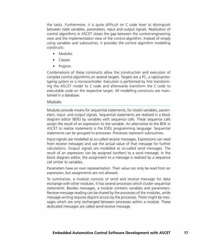
Modules

Modules provide means for sequential statements, for (state) variables, param-eters, input- and output signals. Sequential statements are realized in a blockdiagram editor (BDE) by variables with sequence calls. These sequence callsassign the result of an expression to the variable. An alternative to the BDE inASCET to realize statements is the ESDL programming language. Sequentialstatements can be grouped to processes. Processes represent subroutines.

Input-signals are modelled as so-called receive messages. Expressions can readfrom receive messages and use the actual value of that message for furthercalculations. Output signals are modelled as so-called send messages. Theresult of an expression can be assigned (written) to a send message. In theblock diagram editor, the assignment to a message is realized by a sequencecall similar to variables.

Parameters have an own representation. Their value can only be read from anexpression, but assignments are not allowed.

To summarize, a module consists of send and receive message for dataexchange with other modules. It has several processes which cluster sequentialstatements. Besides messages, a module contains variables and parameters.Receive-message reading can be shared by the processes of the modules, whilemessage-writing requires disjoint access by the processes. There might be mes-sages which are only exchanged between processes within a module. Thesededicated messages are called send-receive message.


18

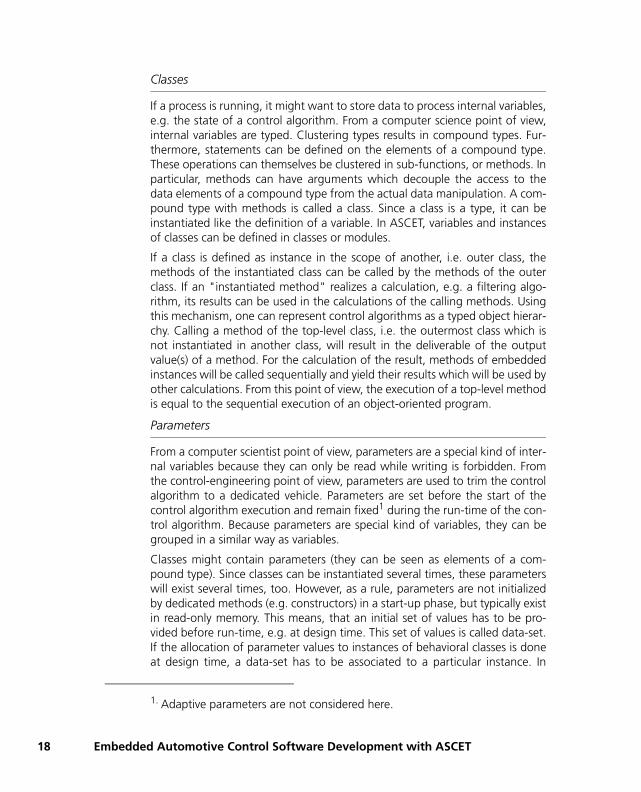
Classes

If a process is running, it might want to store data to process internal variables,e.g. the state of a control algorithm. From a computer science point of view,internal variables are typed. Clustering types results in compound types. Fur-thermore, statements can be defined on the elements of a compound type.These operations can themselves be clustered in sub-functions, or methods. Inparticular, methods can have arguments which decouple the access to thedata elements of a compound type from the actual data manipulation. A com-pound type with methods is called a class. Since a class is a type, it can beinstantiated like the definition of a variable. In ASCET, variables and instancesof classes can be defined in classes or modules.

If a class is defined as instance in the scope of another, i.e. outer class, themethods of the instantiated class can be called by the methods of the outerclass. If an "instantiated method" realizes a calculation, e.g. a filtering algo-rithm, its results can be used in the calculations of the calling methods. Usingthis mechanism, one can represent control algorithms as a typed object hierar-chy. Calling a method of the top-level class, i.e. the outermost class which isnot instantiated in another class, will result in the deliverable of the outputvalue(s) of a method. For the calculation of the result, methods of embeddedinstances will be called sequentially and yield their results which will be used byother calculations. From this point of view, the execution of a top-level methodis equal to the sequential execution of an object-oriented program.

Parameters

From a computer scientist point of view, parameters are a special kind of inter-nal variables because they can only be read while writing is forbidden. Fromthe control-engineering point of view, parameters are used to trim the controlalgorithm to a dedicated vehicle. Parameters are set before the start of thecontrol algorithm execution and remain fixed1 during the run-time of the con-trol algorithm. Because parameters are special kind of variables, they can begrouped in a similar way as variables.

Classes might contain parameters (they can be seen as elements of a com-pound type). Since classes can be instantiated several times, these parameterswill exist several times, too. However, as a rule, parameters are not initializedby dedicated methods (e.g. constructors) in a start-up phase, but typically existin read-only memory. This means, that an initial set of values has to be pro-vided before run-time, e.g. at design time. This set of values is called data-set.If the allocation of parameter values to instances of behavioral classes is doneat design time, a data-set has to be associated to a particular instance. In

1. Adaptive parameters are not considered here.


ASCET, at design time of the class, the data-sets for tentative instances have tobe defined, too, while the association to a particular instance is done when theinstance is created.

Employing Classes in Modules

As written above, the sequential execution of a control algorithm starts withcalling the method of a top-level class. This method call is initiated by the exe-cution of a process. The arguments of a method are typically fed by the receivemessages of the process, while the return value of the method will be fed to asend-message (Of course, these methods might also be fed by internal vari-ables of a module).

From a real-time perspective, the process calling a method of a top-level classgenerates a sequential call-stack of methods which belong to encapsulatedinstances. Even the methods of leave instances are executed in the context ofthe task the process is mapped to. Making the call-stack of methods deepmight compromise reactivity to events. Therefore, when designing classes andemploying them into real-time components, one has to find an appropriatebalance between object-oriented reusability and reactiveness in a task-sched-ule.

Continuous Time Blocks for Plant Modelling

ASCET provides dedicated blocks for the modelling of continuous time sys-tems. These continuous-time blocks (CT blocks) have two flavors:

• Structure blocks which group elementary blocks, and

• Basic blocks which describe the dynamics of elementary systems

Basic blocks assume a non-linear system in normal form of

and specify the dynamic behavior in an object oriented manner. There is aninitialization and termination method, input, update and derivative methods torealize f as well as direct and non-direct output methods to realize g. Further-more, there is a state-event detection method as well as an event methoddescribing what to do in case of a state-event. Last but not least there is amethod to resolve dependent parameters. The expressions can either beexpressed by using the ESDL or C syntax.

),(),(uxgyuxfx

==&


20

Projects for Closed-Loop Simulations

An ECU composition is a set of communicating modules and an operating sys-tem. The operating system configuration defines the tasks and their schedule,while the operating system itself realizes the tasks as well as the messages. Thetask-schedule contains the assignment of processes to tasks. To performclosed-loop simulations on a PC, CT blocks (cf. section "Continuous TimeBlocks for Plant Modelling" on page 19) are attached to the real-time compo-nents of the control algorithm. Binding between the messages of the real-timecomponents and the CT blocks has to be done explicitly, i.e. by connectingports graphically and not by name-matching. The methods of a CT block arecalled from the numerical integration algorithms. The integration algorithmswill be executed as separate task in the resulting operating system configura-tion.

After mapping the processes to tasks and creating the appropriate CT blocktasks, the OS configuration will be translated to executable code. In case of aclosed-loop simulation on a PC, a simulation environment with appropriateevent queues and numerical solvers will be generated. The simulation environ-ment is no real-time execution environment.

2.1.2 Rapid Prototyping

Unfortunately, the employed plant models are typically not detailed enough toserve as a unique reference throughout the design process. Therefore, the con-trol algorithm has to be checked in a real vehicle. This is the first time thecontrol algorithm will run in real-time. The execution entry points of the soft-ware components are mapped to operating system tasks while dedicated soft-ware components for hardware access have to be created and connected withthe software components of the control algorithm. This step is shown inFig. 2-1 on page 15 in linking the logical system architecture to the real vehiclewhich is driven by a driver in a real environment, represented by the arrowlabelled 2. There are many ways to realize this step. First of all, one can use adedicated rapid prototyping system with dedicated I/O boards to interface withthe vehicle. The rapid prototyping systems (RP system) consist of a powerfulprocessor board and I/O boards. The boards are connected via an internal bus-system, e.g. VME. Compared to a production ECU, these processor boards arein general more powerful; they have floating point arithmetic units, and pro-vide more ROM and RAM. Interfacing with sensors and actuators via bus-con-nected boards provides flexibility in different use cases. For short, priority is onrapid prototyping of control algorithms and not on production cost of ECUs.

The interfacing needs of the rapid prototyping systems often result in dedi-cated electrics on the boards. This limits flexibility, and an alternative is there-fore to interface to sensors and actuators using a conventional ECU with itsmicrocontroller peripherals and ECU electronics. A positive side-effect is that


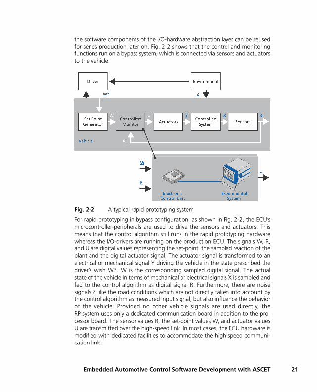
the software components of the I/O-hardware abstraction layer can be reusedfor series production later on. Fig. 2-2 shows that the control and monitoringfunctions run on a bypass system, which is connected via sensors and actuatorsto the vehicle.

Fig. 2-2 A typical rapid prototyping system

For rapid prototyping in bypass configuration, as shown in Fig. 2-2, the ECU’smicrocontroller-peripherals are used to drive the sensors and actuators. Thismeans that the control algorithm still runs in the rapid prototyping hardwarewhereas the I/O-drivers are running on the production ECU. The signals W, R,and U are digital values representing the set-point, the sampled reaction of theplant and the digital actuator signal. The actuator signal is transformed to anelectrical or mechanical signal Y driving the vehicle in the state prescribed thedriver’s wish W*. W is the corresponding sampled digital signal. The actualstate of the vehicle in terms of mechanical or electrical signals X is sampled andfed to the control algorithm as digital signal R. Furthermore, there are noisesignals Z like the road conditions which are not directly taken into account bythe control algorithm as measured input signal, but also influence the behaviorof the vehicle. Provided no other vehicle signals are used directly, theRP system uses only a dedicated communication board in addition to the pro-cessor board. The sensor values R, the set-point values W, and actuator valuesU are transmitted over the high-speed link. In most cases, the ECU hardware ismodified with dedicated facilities to accommodate the high-speed communi-cation link.


22

From the software development point of view, structured interfaces of thesoftware running on the production ECU as well as in the control algorithmdevelopment improves the efficiency of rapid prototyping considerably.

Realtime-I/O Module

For rapid prototyping experiments, dedicated hardware will be used. Besides ahigh-performance microprocessor, there are means available for communica-tion and I/O. For example, in the ETAS ES1000 family the above mentionedmeans are available as VME boards and communication is done via a VME bus.

From a certain point of view, a rapid prototyping system represents a reconfig-urable embedded system. In particular, the communication and I/O hardwarefacilities need basic software modules as glue between the hardware and thecontrol algorithm. These basic software modules are configurable. In ASCET,all basic software modules for the communication and I/O are represented inone ASCET module, the so-called realtime-I/O module. For example, there willbe a process reading signals from the CAN buffer and providing the signals assend-message. This process will be scheduled in an operating system task. Thesignal name as well as the CAN-frame ID can be configured in an editor before.

If a control algorithm shall be tested on an ETAS rapid prototyping system, therealtime-I/O module has to be generated from the configuration parameters. Itis represented as generic ASCET C module and has to be attached to the otherreal-time components, i.e. ASCET modules, to form a running rapid prototyp-ing control algorithm.

Projects for Rapid Prototyping

A project for rapid prototyping does not contain a plant-model represented bycontinuous time blocks. Instead, it contains a real-time I/O module. This real-time I/O module is configured for the rapid prototyping project. On the modellevel, the module communicates with the control algorithm modules via mes-sages. Depending on the configuration of the real-time I/O module, there areseveral processes to be hooked to an operating system task.

2.1.3 Implementation and ECU Integration of Control Algorithms

After the rapid-prototyping step, the control algorithm is valid for use in thevehicle. The code which was generated for rapid prototyping systems relied onthe special features of the processing board, such as RAM resources and thefloating point unit. To make the control algorithm executable under limitedmemory and computational resources, the model of the control algorithm hasto be re-engineered. For example, computation formulas are transformed fromfloating point to fixed point control algorithms, and efficiency, scalability, mod-ularity and other concerns are addressed. The adapted design can be automat-ically transformed to production code in a code generation step.


Floating-Point to Fixed-Point Conversion

A physical plant, e.g. a vehicle, deals with physical quantities, like vehicle-speed and acceleration, coolant temperature, yaw-rate, battery voltage a.s.o.In simulation models, these physical quantities are realized by variables of typefloat, either in 64 or 32 bit guise. The simulation models represent a closed-loop control system, and means that both the vehicle model as well as themodel of the control algorithm are represented in floating point. However,floating point units are expensive and their use in automotive micro-controllersis not common. This means, implementation of a control algorithm on anautomotive micro-controller involves a floating-point to fixed point conversion.

Example: The coolant temperature might range from -50° Celsius to150° Celsius. Fitting these values to an 16-bit integer straight forward wouldbe quite inefficient. Only 0.3% of the available bits would be used as shown inFig. 2-3(a), and the resolution of the temperature would only be 1° Celsius perBit, resulting in a measured temperature of 83.4° Celcius, which is representedas 80° Celsius in the control software.

This can be changed by multiplying every temperature value by 217.78 thushaving a resolution of approximately 0.0046° Celsius per Bit, as shown inFig. 2-3(b). Unfortunately, this adaptation will end up in a floating-point mul-tiplication itself and is not therefore not desirable.

An alternative would be to limit the resolution to 0.0078125° Celsius per bit.Now the multiplication operation can be expressed by a 7bit left-shift opera-tion. Applying this operation to the temperature range yields bit-patterns from-6400 to 19200, thus using a 16 bit integer variable by 39%. This scaling isshown in Fig. 2-3(c).

An even better utilization can be achieved by using an unsigned 16-bit integervalue and a resolution of 0.00390625° Celsius per bit with an offset. This off-set is set to -12800. The temperature range can now be used from -12800 to


24

38400, thus using a range from 51200 values and hence provides a utilizationof more than 78%, as shown in Fig. 2-3(d). However, the offset requires anadditional subtraction.

Fig. 2-3 Unscaled Mapping (a), Aribtrary Mapping (b), 27 Scaling (c), 28 Scaling with Offset (d)

The relationship can be expressed by the linear relationship:

Impl_value = f_impl(phys_value) = phys_value*256+12800

or, more generally, by

impl=scal * phys_value + x

where scal is the scaling factor and x the offset. The resolution is the recip-rocal scaling factor, which means that the physical value is represented by animplementation value of

phys_value = impl_value / scal - ofs

150

0

150

Physical Value Domain Integer Domain (int16)150

0

150Physical Value Domain Integer Domain (int16)

150

0

150

Physical Value Domain150

0

Integer Domain (uint16)

150

(a)

(c) (d)

Integer Domain (int16) Physical Value Domain

(b)

- 150---

- 50---

-50--- 50---

- 50

-50

- 150

- 50 - 50

32767

0

- 32768---

- 50---

32767

0

19200

-32768

-19200---

32767

0

-32768---

-10889

65536

0

51200


Arithmetic with Fixed-Point Values

Associating an implementation formula to every variable has a heavy impacton the statements, i.e. expressions and assignments, of methods or processes.Even the simple assignment of two variables representing physical values

a = b

is not a trivial operation if the implementations, i.e. the associated implemen-tation formulae, are different. Let a and b be implemented by the followingimplementation formulae as unsigned 8 bit variables (range from 0 to 255):

a = 2 * a_impl, b = 3 * b_impl

meaning that the physical value of a has a resolution of 2 while the physicalvalue of b has a resolution of 3. Representing the assignment a=b in imple-mentation terms yields:

2* a_impl = 3* b_impl

This is followed by a simple substitution:

a_impl = (3 / 2)* b_impl

Compared to the original statement a=b, we have now an adapted statementa_impl = (3/2) * b_impl. With respect to implementation formulae1,the adaptations are merely arithmetic operations with constants. However,care must be taken with the series of adaptive operations in order to considerthe requirement for maximum precision. If one, as shown above, first performsthe division, the various conversion equations would be ineffective due to theinteger computation, and the results would be about 50% incorrect. A betterway to express the adapted statement would be:

a_impl = 3 * b_impl / 2

As a result, statements of physical variables adapted by implementation oper-ations often take into account more than just a simple operation.

The question of overflow must be taken into account. This means that if onefirst multiplies by 3, there is an overflow as soon as b_impl becomes greaterthan 255 / 3 = 85. Similarly, one must always be careful of underflows androunding errors. If one first divides by 2, this is equivalent to a right shift oper-ation, i.e. the last bit is dropped. No distinction can then be made whetherb_impl has the value 1 or 0. In both cases, the result for a_impl and thusalso for a is the value 0. In fact, the assignment a = b only makes sense if thephysical ranges are identical (here max. 0 to 510). b_impl can thereforeassume the maximum value 510 / 3 = 170. An overflow can occur here andmust be avoided at all cost. One might think of making a case distinction in the

1. At least the formulae ASCET supports


26

code generation, i.e. first multiply for values from b_impl to 170 and firstdivide for values from b_impl greater than 170. But this leads to a require-ment for more code. So here, one must accept a negligible error in precisionof max. 1.5. within the entire value range. It is clear that the situation itself canbecome more difficult with regular arithmetic operations with few operands,not to mention complex links and expressions.

C Code Classes and Modules

For the migration of legacy code or for micro-controller peripheral access, onemight define classes with the internal behavior of the method specified inC code as well as modules with the internal behavior of processes specified inC. Both C code classes and C code modules already represent implementedcode. This code will be integrated verbatim into the executable for the target.Therefore, C code classes and modules are target-dependent. If one changesthe target of a project, one has to provide the C code for the actual target too.

Projects for Embedded Microcontrollers

As written above, C code classes and modules can be used to access theperipherals of a microcontroller. The ASCET project editors allow to fully con-figurate and generate an operating system. Together with the modules repre-senting the control algorithms, projects for embedded microcontrollers can beused as integration platform. In this case, the code generator will examine theOS schedule and the message communication between the modules and gen-erate the tasks, the messages and the access-code1 of processes to messages.The resulting C code for the project and all its contained modules can be trans-formed to a *.hex file and flashed onto the microcontroller. Needless to saythat an ASAP2 file will be generated too containing all variables to be mea-sured as well as all parameters to be calibrated.

However, there are many cases where a build environment and dedicatedbasic software modules are used for a series production ECU. In this case, typ-ically only the application software, i.e. the control algorithm, is modelled inASCET2. The messages are generated—including the access code of pro-cesses—as well as so-called task bodies, i.e. a sequence of processes as speci-fied in the OS editor. This task body can then be copied to an appropriateOS configuration editor (external to ASCET).

1. Typically realized as macro2. This use-case is often called additional programmer


2.1.4 Reuse of the Control Algorithm in Different Kinds of Projects

As written above, all ASCET modelling elements are maintained in a data-base.Furthermore, projects for different targets differ in the number and kind ofmodules for the same control algorithm.

• Project for closed-loop simulation: This project references the modules for the control algorithm as well as CT blocks.

• Project for rapid prototyping: This project references the modules for the control algorithm (which are the same modules as for the closed-loop simulation) and the realtime-I/O module. The configuration data for the realtime-I/O module is kept at the project

• Project for embedded microcontroller: This project references the mod-ules for the control algorithm as well as the (C code) modules for the peripheral access. If one wants to obtain fixed-point code, one has to attach implementation formulae to modules, classes and projects. Before generating code, one has to the select the appropriate imple-mentation for the project.

ASCET projects can be executed on different execution targets, which mightbe a PC, a rapid prototyping system, or a production ECU1. To run experi-ments, ASCET provides an integrated experiment environment (or EE for short)if the project runs on a PC or rapid-prototyping system. For ECU experiments,an EE is integrated in the measurement and calibration system INCA2 becauseECU experiments are to some extent similar to the fine-tuning3 of a controlalgorithm in the vehicle.

From a software perspective, there are four kinds of experiments:

1. Physical Experiment

2. Quantized Experiment

3. Implementation Experiment

4. Object-Based Controller Implementation Experiment

Only the physical experiment does not need any implementation information.The quantized experiment needs the quantization, the implementation andobject based implementation experiments need additionally the limits and,more important, an integer base type. ASCET control algorithm models are

1. or an evaluation board 2. If the ASCET project consists of CT blocks only and the project runs on a PC

or rapid prototyping hardware, the EE is integrated into LABCAR operator. 3. Because of the limited ECU resources for experimenting, dedicated means

are necessary which are not in the scope of this paper.


28

composed of statements whose generated code looks differently dependingon the type of the target and the selected experiment. In physical experiments,the physical statements will be resolved to real64 variables with no quantiza-tion effects. The quantized experiment uses also real64 variables as basis, butcoerces the physical statements in a way that quantization effects will becomevisible. The implementation experiment uses the full implementation informa-tion and is based on integer types. This means that the types of the variablesin the generated code are the chosen base-types of the implementation andthe operators in the physical statements have been transformed to implemen-tation statements.

The object-based controller implementation experiment uses the types andimplementation statements of the implementation experiment, but the struc-ture of the modules and classes is resolved in a different way. For example, itis possible for every variable in ASCET not only to attach base types, limits andimplementation formulae, but also memory classes. The memory classes reflectthe memory layout of the employed microcontroller. However, as writtenabove, the object-based controller implementation experiment can only bechosen for production ECUs, and online experimentation can only performedby INCA or any other measurement & calibration tool.

When working with a PC or rapid-prototyping target, and all the implementa-tion information w.r.t. base-type, limit, offset and quantization has beenattached to all elements, one can study the effects of implementation formu-lae or integer base types with respect to the physical environment by justswitching the experiment type.

2.1.5 Testing the Technical System Architecture in the Lab

The result of the implementation and integration phase is the technical systemarchitecture, i.e. networked ECUs. These ECUs are tested against plant-modelsin real-time. The plant-models themselves are augmented by models of thesensors and actuators and dedicated boards being able to simulate the electri-cal signals as they are expected by the ECU electronics. These kind of systemsare called Hardware-in-the-Loop systems (or HiL for short) and consist of pro-cessing and I/O boards. The plant model is initialized with different values sim-ulating typical driving manoeuvres. Then, the driving manoeuvre is simulatedon the HiL and providing ECU sensor data as output and accepting ECU actu-ator data as input. This way it can be checked whether the ECU integrationwas successful. HiL testing is represented by the arrow labelled 4 in Fig. 2-1on page 15.


2.1.6 Testing and Honing of the Technical System Architecture in the Vehicle

As written above, there are many use cases where plant models are notdetailed enough to represent the vehicle’s dynamics. Though a lot of calibra-tion activities can nowadays be done by means of HiL-systems, final honing ofa vehicle’s control algorithm still needs to be done with the production soft-ware in a production ECU in a real vehicle. This requires that the technicalsystem architecture is built into a vehicle and tests are done on a provingground. This kind of fine-tuning only concerns the parameter setting of thecontrol algorithm.

2.2 Using ASCET in a Production Environment

Fig. 2-4 Advanced Software Production Environment

In a manual coding environment, there are typically several software develop-ers providing the C code for the control algorithm as well as for the basic soft-ware modules, including the operating system. Then there is an ECU integratorcollecting all necessary source code files and starting the so-called make tool-

Manual C Code(Control Algorithm/

BSW)

GraphicalModeling Tools

BSWConfigurators

.c, .h.c, .h.c, .h.c, .h .c, .h.c, .h.c, .h.c, .h .c, .h.c, .h.c, .h.c, .h

SCMRepository

.c, .h.c, .h.c, .h.c, .h

Make System

.hex


30

chain, which starts the compiler and linker. The C code is transferred betweenthe software developers by using the file-system on the one hand and asource-code management (SCM) system1 on the other. The latter is a databaseholding different versions of the source code files but also allowing the cre-ation and maintenance of configurations. The latter are used as a baseline togenerate/integrate ECU software. To see differences between two versions ofa C code file, difference browsers highlighting the changes in the program textare used. In the last decade, intensive use of SCM systems and differencebrowsing contributed considerably to the enhanced quality of embeddedautomotive software.

In advanced software production environments, some of the C files for controlalgorithms are generated from control algorithm models, e.g. an implementedASCET model, while a lot of C files for basic-software modules, e.g. OS andCOM stack, are generated by so-called configurators. Leaving the ASAM-MCD-2MC file generation aside, such an advanced production environment isshown in Fig. 2-4 on page 29. It shows the C code-generating entities, theSCM database as well as the make system. Looking deeper in such anadvanced production environment, and focussing on the model-based gener-ation of C code for control algorithms with ASCET, one will realize that themodels, which are the basis for the source code, will evolve in the course of thecontrol algorithm development, e.g. incorporating the results of rapid proto-typing. Hence, the models have to be maintained in the SCM database too.

ASCET components are stored in a local database. The local database holdsexact one version of the model. The ASCET-SCM interface establishes a linkfrom the local database to the SCM repository and enables the modelexchange. This model exchange is shown in part (a) of Fig. 2-5 on page 31.Since, in source-code development, difference-browsing between differentversions is indispensable, a similar feature is highly desirable in model-baseddevelopment, too. The ASCET-SCM interface can be enhanced by the so-calledModel-Diff-Browser, thus highlighting, e.g., an additional message in theblock diagram editor of a module.

2.2.1 Model Conversion

As written above, the development of embedded real-time software is drivenboth by control engineers and computer scientists. Sometimes, there aredevelopment processes which start control software development either froma totally behavioral driven point of view or a totally structural driven point ofview, and sometimes even from both views independently of each other.

1. Typical SCM systems are CVS and SubVersion


While ASCET (and AUTOSAR) integrates both approaches with its orthogonalapproach, one might want to take over models stemming from a pure behav-ioral or structural approach.

In the behavioral domain, MATLAB®/Simulink® is a quite popular approach tomodel closed-loop control algorithms without bothering, at least forPC simulation, with too many structuring details. After having performed thePC simulation, the control algorithm parts might be taken over to an ASCETmodule or class as block diagram specification, while the plant parts might berepresented as ASCET CT blocks.

Fig. 2-5 ASCET-SCM interface with (b) and without (a) Diff-Browsing facility

In the structural domain, UML has a certain popularity in both its 1.4 or 2.0guises. Besides very simple class and object diagrams, interaction and collabo-ration diagrams are used to display complex interactions, e.g. in vehicle accesssystems or diagnostics. Sometimes, the classes, objects and their interactionshall be refined in ASCET models so that the natural equivalent in ASCET ofUML, i.e. classes and objects, reflect the object interaction by means ofsequence calls. Embedding the objects in ASCET real-time objects not only addthe real-time perspective to the UML models, but also allow model execution.

(b)

SCMRepository

ASCETDatabase

.c, .h.c, .h.c, .h.c, .h .c, .h.c, .h.c, .h.xml

ASCETASCET

Model Diff.Browser

(a)

SCMRepository

ASCETDatabase

.c, .h.c, .h.c, .h.c, .h .c, .h.c, .h.c, .h.xml

ASCET


32

The model-to-model converter (or M2M for short), a tool provided by the ETASpartner Aquintos, allows these kind of structural and behavioral transforma-tions. It is available for UML 1.4 products and MATLAB/Simulink.

2.3 Summary

Model-based design and implementation of control algorithms is supported byASCET for several development stages. The employed abstraction means allowto use the physical control algorithm model as backbone for all subsequentimplementation annotations throughout the course of development. In partic-ular, no blocks need to be replaced when changing the target. Employing theSCM interface with difference browsing, ASCET can be seamlessly integratedin an ECU production development environment.


3 ASCET and AUTOSAR

This chapter describes the cooperation of ASCET and AUTOSAR. Chapter 3.1overviews the purpose of AUTOSAR, chapter 3.2 describes the AUTOSAR runt-ime environment (RTE), chapter 3.3 lists the AUTOSAR elements supported byASCET.

This chapter contains no detailled introduction to AUTOSAR; see chapter8 "Appendix C: AUTOSAR" on page 161 for more details. The AUTOSAR doc-uments can be found at the AUTOSAR website: http://www.autosar.org/

3.1 Overview

Today, special effort is needed when integrating software components fromdifferent suppliers in a vehicle project comprising networks, electronic controlunits (ECUs), and dissimilar software architectures. While clearly limiting thereusability of automotive embedded software in different projects, this effortalso calls for extra work in order to provide the required fully functional, tested,and qualified software.

By standardizing, inter alia, basic system functions and functional interfaces,the AUTOSAR partnership aims to simplify the joint development of softwarefor automotive electronics, reduce its costs and time-to-market, enhance itsquality, and provide mechanisms required for the design of safety relevant sys-tems.

To reach these goals, AUTOSAR defines an architecture for automotive embed-ded software. It provides for the easy reuse, exchange, scaling, and integrationof those ECU-independent software components (SWCs) that implement thefunctions of the respective application.

The abstraction of the SWC environment is called the virtual function bus(VFB). In each real AUTOSAR ECU, the VFB is mapped by a specific, ECU-dependent implementation of the platform software. The AUTOSAR platformsoftware is split into two major areas of functionality: the runtime environment(RTE) and the basic software (BSW). The BSW provides communications, I/O,and other functionality that all software components are likely to require, e.g.,diagnostics and error reporting, or non-volatile memory management.

ASCET and AUTOSAR 33

http://www.autosar.org/

34

3.1.1 RTA-RTE and RTA-OS

The runtime environment provides the interface between software compo-nents, BSW modules, and operating systems (OS). Concerning the intercon-nection of SWCs, the RTE acts like a telephone switchboard. This is similarlytrue of components that reside either on single ECUs or networked ECUs inter-connected by vehicle buses.

Fig. 3-1 AUTOSAR software component (SWC) communications are rep-resented by a virtual function bus (VFB) implemented through the use of the runtime environment (RTE) and basic software (BSW).

Virtual Function Bus (VFB)

...SWC 3

AUTOSARInterface

SWC 2

AUTOSARInterface

SWC n

AUTOSARInterface

SWC 1

AUTOSARInterface

SWC 1

AUTOSARInterface

SWC 3

AUTOSARInterface

ECU 1

Runtime Environment (RTE)

Basic Software (BSW)

SWC 2

AUTOSARInterface

ECU 2

RTE

BSW

... SWC n

AUTOSARInterface

ECU m

RTE

BSW

GatewayVehicle Bus

ASCET and AUTOSAR

In AUTOSAR, the OS calls the runnable entities of the SWCs through the RTE.RTE and OS are the key modules of the basic software with respect to control-ling application software execution.

ETAS has been supplying the auto industry with automotive operating systemsfor more than a decade: ERCOSEK and now RTA-OSEK. The RTA-RTE AUTOSARRuntime Environment and RTA-OS AUTOSAR Operating System (probablyavailable in the third quarter of 2008) will extend the RTA product portfoliowith support for the key AUTOSAR software modules. RTA-OSEK currentlysupports AUTOSAR OS Scalability Class 1.

Based on their AUTOSAR interfaces, basic software modules from third-partysuppliers can be seamlessly integrated with RTA-RTE and RTA-OSEK.

3.1.2 Creating AUTOSAR Software Components

In addition to an AUTOSAR authoring tool, which provides initial descriptionsof the system architecture and AUTOSAR interfaces, ASCET allows definingand implementing the behavior of AUTOSAR-compliant vehicle functions.

Existing ASCET models can be easily adapted to AUTOSAR because manyAUTOSAR concepts can be mapped to interface specifications in ASCET in asimilar form. On the whole, it suffices to rework the interface of the respectiveapplication to make it AUTOSAR-compliant. As shown in practical demonstra-tions of adapting older models, the expenditure in terms of time is relativelyminor, even with the ASCET version in current use.

ASCET V6.0 supports AUTOSAR SWC descriptions and the generation ofAUTOSAR-compliant SWC production code according to AUTOSAR V2.1.

3.2 What is a Runtime Environment?

The VFB provides the abstraction that allows components to be reusable. Theruntime environment (RTE) provides the mechanisms required to make the VFBabstraction work at runtime. The RTE is, therefore, in the simplest case, animplementation of the VFB. However, the RTE must provide the necessaryinterfacing and infrastructure to allow software components to:

1. be implemented without reference to an ECU (the VFB model); and

2. be integrated with the ECU and the wider vehicle network once this is known (the Systems Integration model) without changing the applica-tion software itself.

More specifically, the RTE must


36

• Provide a communication infrastructure for software components.

This includes both communication between software components on the same ECU (intra-ECU) and communication between software com-ponents on different ECUs (inter-ECU).

• Arrange for real-time scheduling of software components.

This typically means that the runnable entities of the SWC are mapped, according to time constraints specified at design time, onto tasks pro-vided by an operating system.

Application software components have no direct access to the basic softwarebelow the abstraction implemented by the RTE. This means that componentscannot, for example, directly access operating system or communication ser-vices. So, the RTE must present an abstraction over such services. It is essentialthat this abstraction remains unchanged, irrespective of the software compo-nents location. All interaction between software components therefore hap-pens through standardized RTE interface calls.

In addition, the RTE is used for the specific realisation of a previously specifiedarchitecture consisting of SWC on one or more ECUs. To make the RTE imple-mentation efficient, the RTE implementation required for the architecture isdetermined at build time for each ECU. The standardized RTE interfaces areautomatically implemented by an RTE generation tool that makes sure that theinterface behaves in the correct way for the specified component interactionand the specified component allocation.

For example, if two software components reside on the same ECU they can useinternal ECU communication, but if one is moved to a different ECU, commu-nication now needs to occur across the vehicle network.

From the application software component perspective, the generated RTEtherefore encapsulates the differences in the basic software of the variousECUS by:

• Presenting a consistent interface to the software components so they can be reused—they can be designed and written once but used mul-tiple times.

• Binding that interface onto the underlying AUTOSAR basic software implemented in the VFB design abstraction.

3.3 AUTOSAR Elements in ASCET

The following AUTOSAR elements are supported in ASCET:

ASCET and AUTOSAR

3.3.1 AUTOSAR Software Components

AUTOSAR software components are generic application-level componentsthat are designed to be independent of both CPU and location in the vehiclenetwork. An AUTOSAR software component (SWC) can be mapped to anyavailable ECU during system configuration, subject to constraints imposed bythe system designer.

An AUTOSAR software component is therefore the atomic unit of distributionin an AUTOSAR system; it must be mapped completely onto one ECU.

Before an SWC can be created, its component type (SWC type) must bedefined. The SWC type identifies fixed characteristics of an SWC, i.e. portnames, how ports are typed by interfaces, how the SWC behaves, etc. TheSWC type is named, and the name must be unique within the system. Thus, anSWC consists of

• a complete formal SWC description that indicates how the infrastruc-ture of the component must be configured,

• an SWC implementation that contains the functionality (in the form of C code).

To allow an SWC to be used, it needs to be instantiated as configuration time.The distinction between type and instance is analogous to types and variablesin conventional programming languages. You define an application-wideunique type name (SWC type), and delcare one uniquely named variable ofthat type (one or more SWC instance).

3.3.2 Ports and Interfaces

In the VFB model, software components interact trough ports which are typedby interfaces. The interface controlls what can be communicated, as well asthe semantics of communication. The port provides the SWC access to theinterface. The combination of port and port interface is named AUTOSARinterface.

There are two classes of ports:

• Provided ports (Pports) are used by an SWC to provide data or services to other SWC. Pports are implemented either as sender ports or as server ports.


38

• Required ports (Rports) are used by an SWC to require data or services from other SWC. Rports are implemented either as receiver ports or as client ports.

ASCET V6.0 supports one interface type:

• sender-receiver (signal passing)

Each Pport and Rport of an SWC must define the interface type it provides orrequires.

If a system is built from SWC instances, the Rports and Pports of the instancesare connected. One sender must be connected with one receiver.

Sender-Receiver Communication

Sender-receiver communication involves the transmission and reception of sig-nals consisting of atomic data elements sent by one SWC and received by oneor more SWC.

An SWC type can have multiple sender-receiver ports.

Each sender-receiver port can contain multiple data elements each of whichcan be sent and received independently. Data elements within the interfacecan be simple (integer, float, ...) or complex (array, matrix, ...) types.

Sender-receiver communication is one-way; each reply by a receiver must bemodeled as separate sender-receiver communication.

An Rport of an SWC that requires a sender-receiver interface can read the dataelements of the interface. A Pport that provides the interface can write thedata elements.

Sender-receiver communication can be "1:n" (one sender, several receivers)or "n:1" (several senders, one receiver). In the second case, no synchroniza-tion is imposed on the senders.

3.3.3 Runnable Entities and Tasks

A runnable entity is a piece of code in an SWC that is triggered by the RTE (cf.chapter 3.2) at runtime. It corresponds largely to the processes known inASCET.

A software component comprises one or more runnable entities the RTE canaccess at runtime. Runnable entities are triggered, among others, by the fol-lowing events:

Note

In the following, AUTOSAR ports are referred to as Rports or Pports, to avoid confusion with non-AUTOSAR ports.

ASCET and AUTOSAR

• Timing events represent some periodic scheduling event, e.g. a periodic timer tick. The runnable entity provides the entry point for regular exe-cution.

• Events triggered by the reception of data at an Rport (DataReceive events).

AUTOSAR runnable entities can be sorted in several categories. ASCET sup-ports runnable entities of category 1.

In order to be executed, runnable entities must be assigned to the tasks of anAUTOSAR operating system.

3.3.4 Runtime Environment

The runtime environment is described in chapter 3.2.


40
ASCET and AUTOSAR

4 Tutorial

The tutorial mainly addresses users who are new to ASCET. It describes the useof ASCET using practice-oriented examples. The entire tutorial contents aresubdivided into short individual components based on each other. Before youstart working on the tutorial, you should have read chapter "Embedded Auto-motive Control Software Development with ASCET" on page 13.

4.1 A Simple Block Diagram

In ASCET you use components, such as classes and modules, as the main build-ing blocks of your applications. You can either use predefined components,which come with ASCET or have been developed earlier, or create your own,which is what you will be doing in this tutorial.

In ASCET components are usually specified graphically. Once all the compo-nents have been specified, they are assembled into a project, which forms thebasis of an ASCET software system. A software system consists of C code thathas been generated from the graphical model description, and which can berun on a microcontroller or experimental target computer.

4.1.1 Preparatory steps

Before you can start, you have to open a database to work in. All the compo-nents of this tutorial will be stored in this database, so you will only have to dothis once.

All components and projects for this tutorial can be found in the folder calledETAS_Tutorial_Solutions in the database tutorial. It is thereforenot necessary to specify all the components described here yourself .

It is, however, advisable to specify at least the components of lessons one,three and four, to get some practice using ASCET.

Tutorial 41

42

At the start of ASCET, the Component Manager opens, loading the databasethat was last opened.

It is recommended that you create a new database for the tutorial to keep thedata transparent.

To create a new database:

• In the Component Manager, select File → New Database

or

• click on the New button

or

• press <CTRL> + <N>.

The "New database" window opens.

Tutorial

• Enter the name Tutorial.

• Click on OK.

The new database, containing only the data-base name and the Root folder, opens.

To open a database:

When the Tutorial database already exists, proceed as follows:

• In the Component Manager, select File → Open Database

or

• click on the Open button

or

• press <CTRL> + <O>.

The "Open Database" dialog box is displayed. It contains a list of the databases in the current database path.

• If the Tutorial database is on the list, select it and click on OK.

The Component Manager displays the con-tents of the Tutorial database.

• If the Tutorial database is stored some-where else, use the <select path> option to specify the database and click on OK.

• In the "Select database path" window, select the database and click on OK.

The first step in creating your own components is to create a new top levelfolder named Tutorial and a subfolder named LessonN for each lesson.

Tutorial 43

44

To create a new folder:

• In the "1 Database" field, select the database name.

• Select the menu item Insert → Folder

or

• click on the Insert Folder button

or

• press <INSERT>.

A new top-level folder named Root appears in the "1 Database" pane.

• Change the name of the top-level folder to Tutorial. You can type over the highlighted name and then press <ENTER>.

• Select the folder Tutorial.

• Select Insert → Folder once again.

A new folder named Folder is created in the "1 Database" pane.

• Change the name of the new folder to Lesson1.

All the components you create in this tutorial will be stored in a LessonNfolder. You should create a new folder for every lesson. Every database has atleast one top-level folder which can have any number of subfolders.

You can proceed by creating your first component in the Lesson1 folder.

To create a component:

• In the "1 Database" pane, click on the folder Lesson1.

Note

All folder and item names and the names of variables and methods they contain must comply with the ANSI C standard.

Tutorial

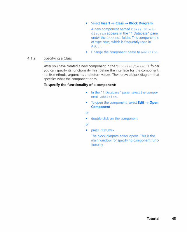
• Select Insert → Class → Block Diagram.

A new component named Class_Block-diagram appears in the "1 Database" pane under the Lesson1 folder. This component is of type class, which is frequently used in ASCET.

• Change the component name to Addition.

4.1.2 Specifying a Class

After you have created a new component in the Tutorial/Lesson1 folderyou can specify its functionality. First define the interface for the component,i.e. its methods, arguments and return values. Then draw a block diagram thatspecifies what the component does.

To specify the functionality of a component:

• In the "1 Database" pane, select the compo-nent Addition.

• To open the component, select Edit → Open Component

or

• double-click on the component

or

• press <RETURN>.

The block diagram editor opens. This is the main window for specifying component func-tionality.

Tutorial 45

46

• In the "Outline" tab, select the method calc. This method is created by default.

• Select Edit → Rename

or

• press <F2>.

The name of the method calc is highlighted.

• Change the name of the method to doAddition.

• Select Edit → Properties

or

Drawing Area

"Components" pane with

"Outline" tab

Palettes

Tutorial

• double-click on the method name.

The signature editor for the method opens.

Every class needs at least one method. Methods in ASCET are similar to meth-ods in object-oriented programming, or functions in procedural programminglanguages. A method can have several arguments and one return value (theseare all optional). Arguments are used to transmit data to a component. Returnvalues are used to return results of calculations within the component to the"outside".

To specify the method signature, you can add two arguments of type con-tinuous and a return value using the signature editor.

To specify the method signature:

• In the signature editor, select Argument → Add.

A new argument called arg appears in the "Arguments" pane.

• Change the name of the argument to input1.

• Add another argument called input2.

By default the data type of the arguments is set to continuous (or cont for short), which is what you need in the example.

Tutorial 47

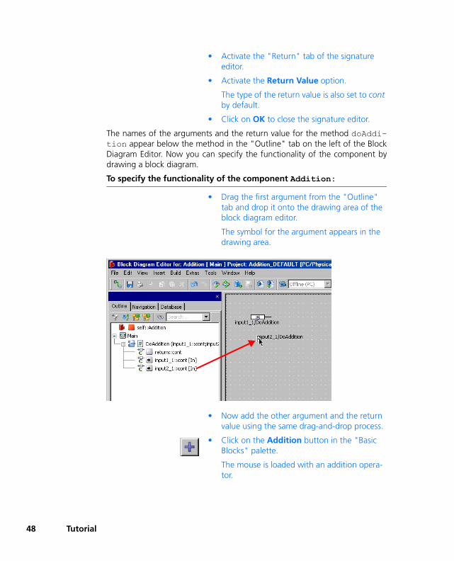
48

• Activate the "Return" tab of the signature editor.

• Activate the Return Value option.

The type of the return value is also set to cont by default.

• Click on OK to close the signature editor.

The names of the arguments and the return value for the method doAddi-tion appear below the method in the "Outline" tab on the left of the BlockDiagram Editor. Now you can specify the functionality of the component bydrawing a block diagram.

To specify the functionality of the component Addition:

• Drag the first argument from the "Outline" tab and drop it onto the drawing area of the block diagram editor.

The symbol for the argument appears in the drawing area.

• Now add the other argument and the return value using the same drag-and-drop process.

• Click on the Addition button in the "Basic Blocks" palette.

The mouse is loaded with an addition opera-tor.

Tutorial

• Click inside the drawing area, between the symbols for the argument and for the return value.

An addition symbol is displayed. By default it has two input pins (indicated by arrows) and one output pin. The output pin is located on the right.

You can now arrange the elements and the operator by dragging them to theirplaces on the drawing area. Next, you need to connect the elements to specifythe flow of information.

To connect the diagram elements:

• Click on the Connect button in the "General" toolbar.

• Alternatively, you can right-click in the draw-ing area (but not on an element).

The cursor changes to a crosshair when it is inside the drawing area.

• Click on the output pin of the first argument symbol to begin a connection.

Now, as you move the mouse cursor, a line is drawn after it. Every time you click inside the drawing area, the line remains fixed up to that point. That way you can determine the path of the connection line

Tutorial 49

50

• Click on the left input of the addition symbol.

The argument symbol is now connected to the input of the addition symbol.

• Connect the second argument symbol with the other input of the addition symbol.

• Connect the return value symbol with the out-put of the addition symbol.

The connection between the addition opera-tor and the return value is displayed as a green line to indicate that the sequencing for this operation needs to be determined.

• Select Tools → Sequence Calls → Sequencing → Ignore Current to determine the addition sequence automatically.

The connection between the addition opera-tor and the return value is displayed as a black line.

Component specification is now complete. The last step in editing your com-ponent is to specify its layout, i.e., the way it is displayed when used withinother components.

Tutorial

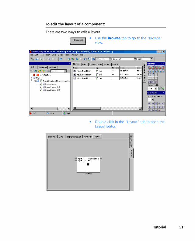
To edit the layout of a component:

There are two ways to edit a layout:

• Use the Browse tab to go to the "Browse" view.

• Double-click in the "Layout" tab to open the Layout Editor.

Tutorial 51

52

• Alternatively, select Edit → Component → Layout.

The Layout Editor opens.

• Resize the block by clicking on it and then dragging the handles to the size you want.

• Drag the pins of the arguments and the return value to create a symmetrical design.

• Click on OK.

Now that you have finished your component, the last step in this lesson is tosave the component in the database.

To save the component Addition:

• Select File → Save and close the block dia-gram editor.

• In the Component Manager, click on the Save button.

Your work is not written to disk until you per-form this operation.

When you select Save in the block diagram editor, the changes are only stored in the cache memory. It is therefore advisable to click Save in the Component Manager regularly as work progresses.

You can have your changes saved automati-cally by activating the appropriate user options (see the ASCET online help) for your ASCET session.

Tutorial

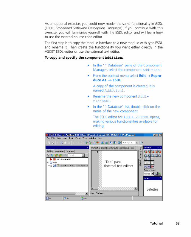
As an optional exercise, you could now model the same functionality in ESDL(ESDL: Embedded Software Description Language). If you continue with thisexercise, you will familiarize yourself with the ESDL editor and will learn howto use the external source code editor.

The first step is to copy the module interface to a new module with type ESDLand rename it. Then create the functionality you want either directly in theASCET ESDL editor or use the external text editor.

To copy and specify the component Addition:

• In the "1 Database" pane of the Component Manager, select the component Addition.

• From the context menu select Edit → Repro-duce As → ESDL.

A copy of the component is created; it is named Addition1.

• Rename the new component Addi-tionESDL.

• In the "1 Database" list, double-click on the name of the new component.

The ESDL editor for AdditionESDL opens, making various functionalities available for editing.

"Edit" pane(internal text editor)

palettes

Tutorial 53

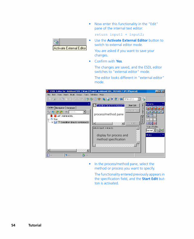
54

• Now enter this functionality in the "Edit" pane of the internal text editor:

return input1 + input2;

• Use the Activate External Editor button to switch to external editor mode.

You are asked if you want to save your changes.

• Confirm with Yes.

The changes are saved, and the ESDL editor switches to "external editor" mode.

The editor looks different in "external editor" mode.

• In the process/method pane, select the method or process you want to specify.

The functionality entered previously appears in the specification field, and the Start Edit but-ton is activated.

process/method pane

display for process and method specification

Tutorial

• Activate the external editor with Start Edit.

The End Edit and Update buttons are now activated, whilst the Start Edit button is deac-tivated.

• Edit the functionality in the external editor.

• Save the functionality in the external editor.

• In the ESDL editor, click Update, to transmit the data from the external editor.

• After you have finished, click End Edit to close the connection to the external editor.

The external editor remains open after you have clicked on End Edit. However, you can-not transmit any more changes to the ESDL editor.

• Click on Activate External Editor a second time to end the external editor mode.

• Select Build → Analyze Diagram to check the code you entered.

Errors are listed in the ASCET monitor win-dow.

4.1.3 Summary

After completing this lesson you should be able to perform the following tasksin ASCET:

• Opening a database

• Creating and naming a folder

• Creating and naming a component

• Defining the interface for a method

• Placing diagram elements on the drawing area

• Connecting diagram elements

Note

When the external editor starts up, the application associated with the file endings *.c and *.h in the operating system register database is called. Data transfer is done via temporary files; this is why you have to ensure the files are saved before closing the editor or before transferring to the ESDL editor.

Tutorial 55

56

• Editing the layout of a component

• Switching between Specification and Browser views.

• Saving a component.

• Copying a component interface.

• Using the ESDL editor.

• Using the external editor.

4.2 Experimenting with Components

Having created the Addition or AdditionESDL components, you cannow experiment with them. Experimentation allows you to see how the com-ponent works, just as it would in a real application. The experimentation envi-ronment provides a variety of tools that can show the values of inputs,outputs, parameters and variables within a component.

4.2.1 Starting the Experimentation Environment

The experimentation environment is called from the block diagram or the ESDLeditor. First open it with the component you want to experiment with.

To start the experimentation environment:

• From the ASCET Component Manager, open the block diagram editor for your Addition in the \Tutorial\Lesson1 folder.

• In the block diagram editor, select Build → Experiment.

The code for the experiment is generated. ASCET analyses the model in your specifica-tion and generates C code that implements the model. It is possible to generate specific code for different platforms.

In your example, you simply use the default settings to generate code for the PC.

After the code has been generated and com-piled, the experimentation environment opens.

Tutorial

4.2.2 Setting up the Experimentation Environment

Before you can start experimenting, you have to set up the environment,which means determining the input values generated for the experiment andhow you want to view the results. You have to carry out three steps. First setup the event generator, then the data generator and finally the measurementsystem.

To set up the Event Generator:

• Click on the Open Event Generator button.

The "Event Generator" window opens. For each method to be simulated, you need to create an event and also a generateData

Tutorial 57

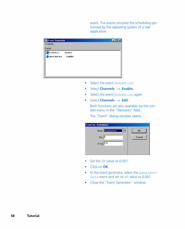
58

event. The events simulate the scheduling per-formed by the operating system of a real application.

• Select the event DoAddtion.

• Select Channels → Enable.

• Select the event DoAddtion again.

• Select Channels → Edit.

Both functions are also available via the con-text menu in the "Elements" field.

The "Event" dialog window opens.

• Set the dT value to 0.001.

• Click on OK.

• In the event generator, select the generate-Data event and set its dT value to 0.001.

• Close the "Event Generator" window.

Tutorial

To set up the Data Generator:

• Click on the Open Data Generator button.

The "Data Generator" window opens.

• Select Channels → Create.

The "Create Data Generator Channel" dialog window opens.

• Select the input1/DoAddition and the input2/DoAddition variables from the list.

• Click on OK.

Now both inputs are listed in the "Data Ele-ments" pane of the "Data Generator" win-dow.

Tutorial 59

60

• Select input1/DoAddition in the "Data Elements" pane.


The "Stimulus" dialog box appears.

• Set the values as follows.

• Click on OK to close the "Stimulus" dialog pane.

• Set the values for input2 as follows:

• Close the "Data Generator" window.

With these settings you get two sine waves with different frequencies and dif-ferent amplitudes. The Addition component adds the two waves and dis-plays the resulting curve.

In order to see the three curves displayed on an oscilloscope, you will now setup a measurement system.

Mode: sine

Frequency: 1.0 Hz

Phase: 0.0 s

Offset: 0.0

Amplitude: 1.0

Mode: sine

Frequency: 2.0 Hz

Phase: 0.0 s

Offset: 0.0

Amplitude: 2.0

Tutorial

To set up the measurement system:

• In the "Physical Experiment" window, select <2. New Oscilloscope> as data display type from the "Measure View" combo box.

• In the "Outline" tab, expand the elements list.

• Select input1/DoAddition.

• Select Extras → Measure.

An oscilloscope window opens with input1 as measurement channel. The "Measure view" list in the experimentation environment is updated to display the title of the measure-ment window.

• In the "Outline" tab of the "Physical Experi-ment" window, select input2/DoAddi-tion.

Tutorial 61

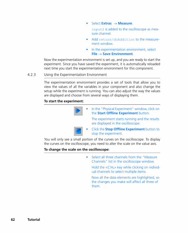
62


input2 is added to the oscilloscope as mea-sure channel.

• Add return/doAddition to the measure-ment window.

• In the experimentation environment, select File → Save Environment.

Now the experimentation environment is set up, and you are ready to start theexperiment. Since you have saved the experiment, it is automatically reloadednext time you start the experimentation environment for this component.

4.2.3 Using the Experimentation Environment

The experimentation environment provides a set of tools that allow you toview the values of all the variables in your component and also change thesetup while the experiment is running. You can also adjust the way the valuesare displayed and choose from several ways of displaying them.

To start the experiment:

• In the "Physical Experiment" window, click on the Start Offline Experiment button.

The experiment starts running and the results are displayed in the oscilloscope.

• Click the Stop Offline Experiment button to stop the experiment.

You will only see a small portion of the curves on the oscilloscope. To displaythe curves on the oscilloscope, you need to alter the scale on the value axis.

To change the scale on the oscilloscope:

• Select all three channels from the "Measure Channels" list in the oscilloscope window.

Hold the <CTRL> key while clicking on individ-ual channels to select multiple items.

Now all the data elements are highlighted, so the changes you make will affect all three of them.

Tutorial

• Select Extras → Setup.

The "Display Setup" dialog box appears.

• Set the "Value Axis" to a range of -3 to 3.

• Set the "Time Axis Extent" to 3.

• Select a background color in the "Background color" list.

• Press <ENTER>.

Tutorial 63

64

The oscilloscope now shows the output with the appropriate scaling on thevalue axis. You will see the two input sine waves, together with the waveresulting from their addition. You can now adjust the input values to see howthe output is affected.

To change the input values for experimentation:

• In the "Physical Experiment" window, select Tools → Data Generator to open the "Data Generator" window.

• In the data generator, select the variable you want to change.


The "Stimulus" dialog window opens.

• Adjust the values you want to change.

• Click Apply.

The curves in the oscilloscope change according to the new settings. You canchange all the settings in the experimentation environment while the experi-ment is running.

4.2.4 Summary


• To call the experimentation environment

• Setting up the event generator

• Setting up the data generator

• Setting up the measuring system

• Starting and stopping the experiment

• Saving the experiment

• Changing stimuli while the experiment is running

4.3 To Specify a Reusable Component

In this lesson you will create a class that implements an integrator, a standardpiece of functionality that is often used in microcontroller software. While thisis a slightly more complex diagram, the techniques for creating and experi-menting with it are the same ones you have learned already.

Tutorial

In this example, you specify an integrator that calculates the distance coveredwhere time and speed are known. The input value will be given in meters persecond, and at each interval multiplied with a dT in seconds. The value foreach time slice is added up in an accumulator. The accumulator stores the dis-tance in meters that has been covered after a certain length of time.

In ASCET, a standard block, such as an accumulator, can be realized with asimple diagram.

4.3.1 Creating the Diagram

Before you start working on the diagram, you need to perform the same stepsas for the addition component. First create a new folder in the Tutorialfolder, then add a new class. Finally, you can specify the interface of the meth-ods, then the block diagram and the layout.

You will start by creating the folder and the new class.

To create the integrator class:

• In the Component Manager, open the Tuto-rial folder.

• Create a new folder and call it Lesson3.

• In the Lesson3 folder, create a new class and call it Integrator.

To define the integrator interface:

• In the "1 Database" pane, select the element Integrator.

• Double-click on the element or select Edit → Open Component.

The block diagram editor opens.

• Rename the method calc to integrate.

Tutorial 65

66

• Edit the method integrate by adding one argument (type cont) and a return value (type cont).

• Place the argument and return value from integrate on the drawing area.

The integrator uses two new types of elements that we have not used before:a variable and a parameter.

Variables are used in the same way as they are used in programming lan-guages; you can store values in them and read the values for further calcula-tions. In contrast, parameters are read-only. They can only be changed fromoutside, e.g. they can be calibrated in the experimentation environment, butthey cannot be overwritten by any of the calculations within the componentitself.

In addition, we want to specify a dependent parameter in this example. How-ever, it is irrelevant for the functionality of the integrator. A dependent param-eter is dependent on one or several parameters, i.e. its value is calculatedbased on a change in another one. The calculation or dependency is only car-ried out on specification, calibration or application. A dependent parameterbehaves in exactly the same way in the target code as a normal parameter.

Tutorial

To create a variable:

• Click on the Continuous Variable button in the "Elements" palette.

The properties editor opens.

• In the "Name" field, enter the name buffer.

• Click OK.

The variable is now named buffer. The cur-sor shape changes to a crosshair. It is loaded with the continuous variable.

• Click inside the drawing area to place the vari-able.

The variable is placed in the drawing area. Its name is highlighted in the "Outline" tab.

When the properties editor does not open automatically, place the variable inthe drawing area. Afterwards, double-click on the variable in the "Outline" tabto open the properties editor manually. Make the required settings and acti-vate the Always show dialog for new elements option. The next time youcreate an element, the properties editor opens automatically.

Tutorial 67

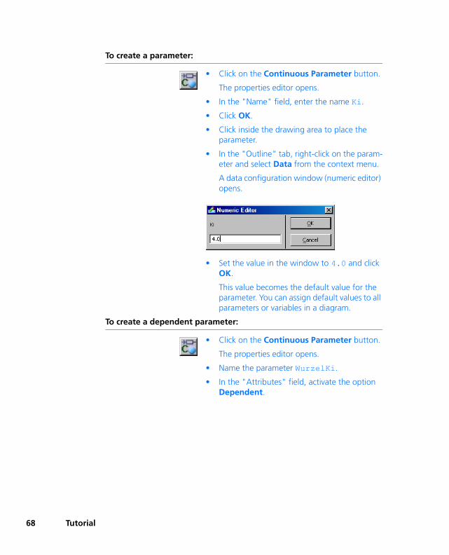
68

To create a parameter:

• Click on the Continuous Parameter button.


• In the "Name" field, enter the name Ki.

• Click OK.

• Click inside the drawing area to place the parameter.

• In the "Outline" tab, right-click on the param-eter and select Data from the context menu.

A data configuration window (numeric editor) opens.

• Set the value in the window to 4.0 and click OK.

This value becomes the default value for the parameter. You can assign default values to all parameters or variables in a diagram.

To create a dependent parameter:

• Click on the Continuous Parameter button.


• Name the parameter WurzelKi.

• In the "Attributes" field, activate the option Dependent.

Tutorial

• Open the formula editor using the Formula button.

• Right-click in the "Identifier" field and select Add from the context menu.

A formal parameter is created.

• In the "Identifier" field, enter the name x for the new parameter.

• In the "Formula" field, specify the calculation rule.

You can select different operators from the "Operator" combo box for more complex for-mulas. They are added to the "Formula" field one by one with the >> button next to the "Operator" field.

Likewise, various functions can be selected in the "Function" combo box, and inserted into the "Formula" field with the >> button next to the "Function" combo box.

• For the example here, select the root calcula-tion of the formal parameter.

Formal Parameter: xFormula: sqrt(x)

• Exit with OK, and close the properties editor, too.

The cursor shape changes to a crosshair.

Tutorial 69

70

• Click into the drawing area to place the parameter.

• In the block diagram editor, right-click on the WurzelKi parameter in the "Outline" tab, and select Data from the context menu.

• In the "Dependency Editor" window, assign a model parameter from the combo box to the formal parameter (in this example Ki).

• Complete data entry with OK.

You have now specified a parameter depen-dent on the parameter Ki which on calibra-tion will automatically be calculated based on Ki. Later on in the experiment, you can check the dependency or the calculation.

Now that you have added all the elements, you need to specify an integrator.You can proceed by creating the remainder of the diagram.

Tutorial

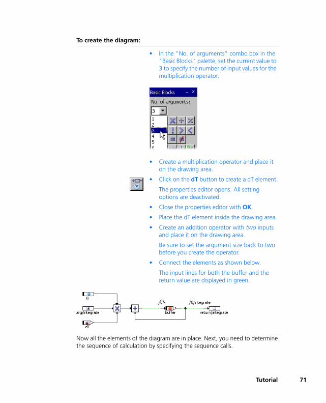
To create the diagram:

• In the "No. of arguments" combo box in the "Basic Blocks" palette, set the current value to 3 to specify the number of input values for the multiplication operator.

• Create a multiplication operator and place it on the drawing area.

• Click on the dT button to create a dT element.

The properties editor opens. All setting options are deactivated.

• Close the properties editor with OK.

• Place the dT element inside the drawing area.

• Create an addition operator with two inputs and place it on the drawing area.

Be sure to set the argument size back to two before you create the operator.

• Connect the elements as shown below.

The input lines for both the buffer and the return value are displayed in green.

Now all the elements of the diagram are in place. Next, you need to determinethe sequence of calculation by specifying the sequence calls.

Tutorial 71

72

To assign a value to a sequence call:

• Right-click on the sequence call above the variable buffer.

• Select Edit from the context menu.

The sequence editor opens.

• Click on OK to accept the default settings.

The assignment comes first in the algorithm for your integrator.

To adjust the sequence number in a sequence call:

• Right-click on the sequence call above the return value for integrate.

• Select Edit from the context menu.

• In the sequence editor, set the value for "Sequence Number" to 2.

Sequence calls

Tutorial

• Click on OK.

The return value is assigned only after the vari-able buffer has been updated.

To adjust the layout:

• Select Edit → Component → Layout.

The layout editor opens.

Alternatively you can also get to the layout editor from the "Information/Browse" view by doubleclicking the layout within the "Layout" tab.

• Drag the argument from integrate to the middle of the left-hand side of the block.

• Drag the return value to the middle of the right-hand side of the block.

• Click on OK.

The diagram for the integrator class is now complete. Now save the changesto the diagram by selecting File → Save in the block diagram editor. Changesthat do not affect the diagram itself are stored automatically. Next, save thechanges to the database by selecting File → Save Database in the Compo-nent Manager window.

4.3.2 Experimenting with the Integrator

Again, first set up the event generator, then the data generator and finally themeasurement system.

Tutorial 73

74

To set up the experimentation environment for the integrator:

• Start the experimentation environment by selecting Component → Offline Experi-ment.

• Click the Event Generator button.

• Activate the event integrate using the default dT value of 0.01.

• Close the "Event generator" window.

• Click on the Data Generator button.

• Create a data channel for the integrate method by selecting Channels → Create and selecting the argument from integrate.

• Set the values as follows:

• Close the Data Generator.

Mode: pulse

Frequency: 0,2 Hz

Phase: 0.0 s

Offset: -1.0

Amplitude: 2.0

Tutorial

• Open an oscilloscope window with the arg and return values from the integrate method.

• Set the value axis to a range from -10 to 10 and the time axis extent to 10 seconds.

• Click on Start Offline Experiment to start the experiment.

The output value of the integrate method increases when the argument ispositive, and decreases when it is negative. Because the positive and negativeparts of the input curve are equal, the output will remain within stable bound-aries.

To reset an experiment:

If you stop an experiment, the current values of variables and parameters arestored; they are used again when the experiment is restarted. It may be desir-able to reset all variables or parameters to their initial values.

• Select Extras → Reinitialize → Variables or Parameters or Both.

Depending on your selection, either all vari-ables or all parameters, or both, are reset to their initialization values.

Next, you should experiment with various settings to illustrate the function ofthe integrator. You can adjust the Ki parameter and change the input.

Tutorial 75

76

To experiment with the integrator:

• In the "Outline" tab, expand the Integra-tor element.

• Select the parameter Ki.

• Select Extras → Calibrate.

A numerical editor opens for the parameter.

• Set the value to 5.

The output curve on the oscilloscope becomes steeper.

• Set the value to 3.

The output curve now becomes flatter again.

• Set the parameter back to 4 and close the numerical editor.

• Open the "Data Generator" window.

• Set the offset of the input pulse to -0.5.

• Click on OK.

Now the positive part is greater, so the output will start to increase. At somepoint it will exceed the oscilloscope limits. You can adjust the scale of the oscil-loscope for each value individually by selecting only that value when you makechanges. You can also open a numerical display window to see the outputvalue.

To display a value numerically:

• Select <1.Numeric Display> in the "Measure View" combo box in the experi-mentation environment.

• In the "Outline" tab, select the return value (return) from the integrate method.


A "Numeric display" window shows the cur-rent return value.

Tutorial

• Also display the dependent parameter Wur-zelKi.

• Experiment with changing Ki and initiating update using the Update Dependent Parameters button.

4.3.3 Summary


• Creating a parameter

• Creating and specifying a dependent parameter

• Creating a variable:

• Creating an operator with multiple inputs

• Setting the sequence number of a sequence call

• Assigning a default value

• Calibrating a value during experimentation

• Displaying values in a "Numeric display" window

4.4 A Practical Example

In this lesson you will create a controller based on a slightly enhanced standardPI filter. The controller will be used to keep the rotational speed of an idling carengine constant.

When controlling the idling speed of an engine, you have to make sure thatthe actual number of revolutions n stays close to the nominal value for idlingn_nominal. The value n is subtracted from n_nominal to determine thedeviation that is to be controlled.

The deviation in the actual number of revolution forms the basis for calculatingthe value of air_nominal, which determines the throttle position, i.e. theamount of air the engine gets.

4.4.1 Specifying the controller

The steps in creating the diagram for your controller are the same as earlier:

• adding a new folder and creating the component in the Component Manager,

• defining the interface and drawing the block diagram.

Tutorial 77

78

The major difference is that you will implement the controller as a module.Modules are used as the top-level components in projects. They define theprocesses that make up a project.

To create the controller component:

• In the Component Manager, add a new sub-folder to the Tutorial folder and rename it Lesson4.

• Select the Lesson4 folder and select Insert → Module → Block diagram to add a new module.

• Rename the new module IdleCon and open the block diagram editor.

• In the "Outline" tab, rename the diagram process to p_idle.

The functionality of modules is specified in processes, which correspond to themethods in classes. Unlike methods, processes do not have arguments orreturn values. Data exchange (communication) between processes is based ondirected messages, which are referred to as Receive messages (inputs) andSend messages (outputs) in ASCET.

In your controller, you will use a receive message to process the actual numberof revolutions n and a send message to adjust the throttle position toair_nominal.

To specify the interface of the controller:

• Create a receive message by clicking on the Receive Message button and name it n.

• In the properties editor for the message n, activate the Set() Method option.

• Click on the Send Message button and then inside the drawing area to create a send mes-sage.

Tutorial

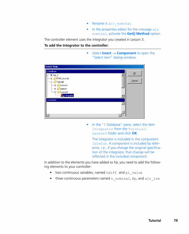
• Rename it air_nominal.

• In the properties editor for the message air nominal, activate the Get() Method option.

The controller element uses the integrator you created in Lesson 3.

To add the Integrator to the controller:

• Select Insert → Component to open the "Select item" dialog window.

• In the "1 Database" pane, select the item Integrator from the Tutorial\ Lesson3 folder and click OK.

The integrator is included in the component IdleCon. A component is included by refer-ence, i.e., if you change the original specifica-tion of the integrator, that change will be reflected in the included component.

In addition to the elements you have added so far, you need to add the follow-ing elements to your controller:

• two continuous variables, named ndiff and pi_value

• three continuous parameters named n_nominal, Kp, and air_low

Tutorial 79

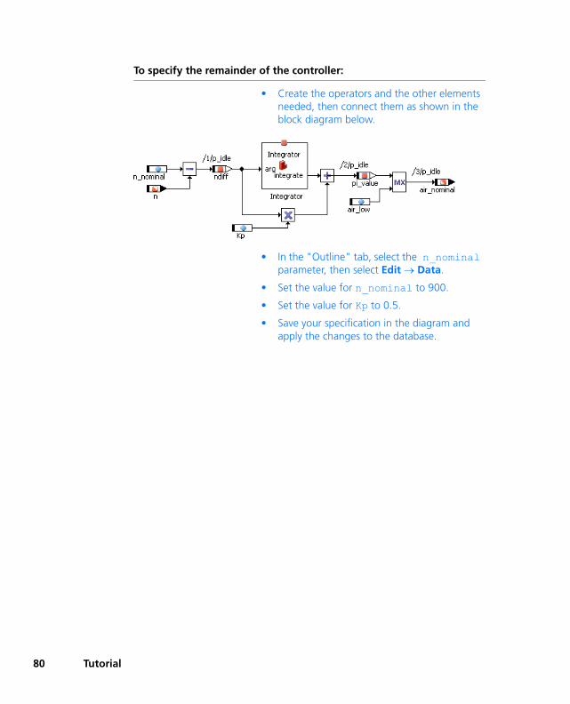
80

To specify the remainder of the controller:

• Create the operators and the other elements needed, then connect them as shown in the block diagram below.

• In the "Outline" tab, select the n_nominal parameter, then select Edit → Data.

• Set the value for n_nominal to 900.

• Set the value for Kp to 0.5.

• Save your specification in the diagram and apply the changes to the database.

Tutorial

4.4.2 Experimenting with the Controller

Experimentation with modules works like experimentation with other compo-nents. First the data and event generators and then the measurement systemare set up.

To set up the experimentation environment:

• Select Build → Experiment to start the experimentation environment.

• Open the "Event Generator" window and enable the event for the process p_idle using the default value of 0.01 for dT.

An event for a process works the same as an event for a method.

• Open the "Data generator" window and set up the channel for the receive message n with the following values:

Mode: pulse

Frequency: 1.0 Hz

Tutorial 81

82

• Set up an oscilloscope with the variables n_diff and air_nominal.

• In the oscilloscope, set the value axis to -500 to 500 and the time axis extent to 2.

• Click on the Save Environment button.

The experiment is now set up to display the relationship between the deviationin the number of revolutions and the throttle position.

To experiment with the controller:

• Start the experiment by clicking the Start Offline Experiment button.

• Open a calibration window for the variables Ki and Kp. From here, you can adjust the val-ues Ki and Kp and observe their effect on the output.

From time to time, you may need to reinitialize the model in order to get back to meaningful values.

4.4.3 A Project

A project is the main unit of ASCET software representing a complete softwaresystem. This software system can be executed on experimental or microcon-troller targets in real-time with an online experiment. Individual componentscan only be tested in the offline experimentation environment.

Phase: 0.0

Offset: 800.0

Amplitude: 200.0

Tutorial

Every experiment runs in the context of a project. Whenever code is generatedfor a project, the operating system code is also generated. The operating sys-tem specification is required to run on an ASCET software system in real-time.Running a software system in real-time is called Online experimentation. So far,we have experimented offline only, i.e. not in real-time.

4.4.4 To set up the Project

The project is created in the Component Manager. You can add it to the samefolder as the IdleCon module.

To create a project:

• In the Component Manager, select Insert → Project or click on Insert Project to add a new project.

• Name the project ControllerTest.

• Select Edit → Open Component or double-click the project.

The project editor opens for the project.

Note

All ASCET experiments—both online and offline—run within the context of a project. This is clearly seen with offline experiments, which use an (other-wise invisible) default project. Creating and setting up a project for the express purpose of specifying an operating system is only required for online experiments. However, you also have the option of configuring the default project for your own application.

Tutorial 83

84

The next step is to add the IdleCon controller to the "Outline" tab of theproject.

To include components in a project:

• In the project editor, select Insert → Compo-nent to open the "Select item" dialog win-dow.

• From the "1 Database" list, select the compo-nent IdleCon in the Tutorial\Lesson4 folder.

• Click on OK to add the component.

The name of the component is shown in the "Outline" tab of the project editor.

Components are included by reference, i.e. if you change the diagram of anincluded component, that change will also be effective in the project.

The operating system schedules the tasks and processes of a project. Beforeyou can generate code for the project, you have to create the necessary tasksand assign the processes to them.

The operating system schedule is specified in the "OS" tab of the project edi-tor. You will now specify the operating system schedule to have the p_idleprocess activated every 10 ms.

Tutorial

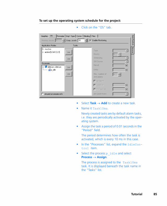
To set up the operating system schedule for the project:

• Click on the "OS" tab.

• Select Task → Add to create a new task.

• Name it Task10ms.

Newly created tasks are by default alarm tasks, i.e. they are periodically activated by the oper-ating system.

• Assign the task a period of 0.01 seconds in the "Period" field.

The period determines how often the task is activated, which is every 10 ms in this case.

• In the "Processes" list, expand the IdleCon-trol item.

• Select the process p_idle and select Process → Assign.

The process is assigned to the Task10ms task. It is displayed beneath the task name in the "Tasks" list.

Tutorial 85

86

In projects, imported and exported elements are used for inter-process com-munication. They are global elements that correspond to the send and receivemessages in the modules. Global elements must be declared in the project andlinked to their respective counterparts in the modules included in the project.

To define global elements:

• In the project editor, select Extras → Global Elements → Resolve Globals.

The necessary global elements are created and automatically linked to their counterparts. Ele-ments with the same name are automatically linked to each other.

4.4.5 Experimenting with the Project

You will now run an offline experiment with this project. Offline experimenta-tion can be performed on the PC without the connection of any additionalhardware. Projects run on the PC by default. Therefore you do not have toadjust any settings. Offline experimentation with projects works like offlineexperimentation with components.


• In the Component Manager, select File → Save Database.

It is always a good idea to apply your changes to the database before you start the experi-mentation environment.

• In the project editor, select Build → Experi-ment.

Code for the project is generated and the offline experimentation environment opens.

Tutorial

• Click on the Open Event Generator button.

In the event generator you see an event for each task you want to use in the experiment, rather than for each method or process, as in experimentation with components.

• Enable the task generateData from the event generator and use the default dT value of 0.01 seconds.

The task Task10ms is already enabled by default, and both events now have 0.01 sec-onds as their dT value; therefore you do not need to make any further adjustments.

• Close the event generator.

• Set up the data generator and measurement system with the same values as in the previous experiment (cf. "Experimenting with the Con-troller" on page 81).

• Save the environment by selecting File → Save Environment.

Tutorial 87

88

To run the experiment:

• Click on the Start Offline Experiment but-ton.

• Adjust the Ki and Kp parameters as in the previous section to see the effect of your changes in the output.

4.4.6 Summary


• Creating modules

• Creating messages in modules

• Using components from the Component Manager in a block diagram.

• Creating a project

• Including components in projects.

• Creating tasks and assigning processes to them

• Experimenting with projects

4.5 Extending the Project

In this lesson you will add some refinements to make your controller morerealistic. You will create a signal converter that converts sensor readings intoactual values. Many sensors, used for instance in automotive applications,return a voltage that corresponds to a particular measurement value, such astemperature, position or number of revolutions per minute. The relationshipbetween the voltage and the measured value is not always linear. ASCET pro-vides characteristic tables to model this kind of behavior efficiently.

4.5.1 Specifying the Signal Converter

The first step in modeling the signal converter is to create a folder and a mod-ule that specifies the functionality. The signal converter uses two characteristiclines to map its input values to the corresponding outputs.

To create the module:

• In the Component Manager, create a new folder Tutorial\Lesson5.

• Create a new module and name it SignalConv.

Tutorial

• Double-click the element to open the block diagram editor.

• In the block diagram editor, select Insert → Process to create a second process.

• Name the processes n_sampling and t_sampling.

• In the "Outline" tab, create two receive mes-sages U_n and U_t and two send messages t and n.

• Create a characteristic field by clicking on the OneD Table button.


• Call the table t_sensor.

• In the "x" part of the "Dimension" field, enter the value 13.

The characteristic field can now span a maxi-mum of 13 columns.As you have created a one-dimensional char-acteristic line, the "y" part of the "Dimen-sion" field is inactive.

• Click OK to close the properties editor.

• Then click in the drawing area to place the table.

The table is added to the "Outline" tab.

• Create a second table with a maximum of 2 columns and call it n_sensor.

• Connect the elements as shown and edit the sequencing to assign the corresponding pro-cesses.

Tutorial 89

90

The next step is to edit the data for the two characteristic fields. ASCET pro-vides a table editor for editing arrays, matrices and characteristic fields.

To edit the tables:

• Right-click on the table t_sensor and select Data from the context menu.

The table editor opens.

• Adjust the size of the table as follows:

The table is extended to 13 columns with all z-values set to 0 by default.

• Enter the values listed in the following table. The top row corresponds to the X row, the bottom row to the Z row.

You should edit the table by entering the sam-ple points (X values) first, starting from left to right.

• Click on an X value and then enter the new one in the dialog box.

The new X value must be between the limits set left and right by the sample points.

• Then enter the output values by clicking on a value and typing over the highlighted value.

• Edit the second table in the same way using the following data:

• In the block diagram editor, select File → Save.

• In the Component Manager, click on the Save button to store your changes.

0.00 0.08 0.30 0.67 1.17 2.5 5.00 7.50 8.83 9.33 9.70 9.92 10.00

-40.0 -26.0 -13.0 0.0 13.0 40.0 80.0 120.0 146.0 160.0 173.0 186.0 200.0

0.0 10.0

0.0 6000.0

Tutorial

In this example, the second table represents a linear relationship betweeninput and output, therefore it needs only two sample points. This worksbecause you have specified the interpolation mode between values as linear.

In linear interpolation, for an input value between two sample points the out-put value is determined from a straight line. In this case, an input of 0 returns0 and an input of 10 returns 6000. If the input value is 5, the return value isinterpolated accordingly as 3000.

4.5.2 Experimenting with the Signal Converter

You can now experiment with the new component to observe the behavior ofthe tables. Since the two tables have different value ranges, you will set up aseparate oscilloscope window for each of them.


• Select Build → Experiment to open the experimentation environment.

• Create an event for each process in the com-ponent (n_sampling, t_sampling, generateData) and assign a dT value of 4 ms to each event.

Tutorial 91

92

• In the data generator create a channel for the message U_n and one for U_t and set up both channels with the following values:

• Create an oscilloscope window with the mes-sages n and U_n and a second oscilloscope with the messages t and U_t.

Before you create the second oscilloscope, be sure to activate the <2. New Oscillo-scope> entry in the "Select Measure View" combo box.

The resolution of the sampling points and their corresponding interpolationvalues differs so much that you should configure each channel in the two oscil-loscopes individually in order to optimize the way the behavior of the twotables is displayed.

To set up the oscilloscopes for measuring:

• Activate the oscilloscope for the process n_sampling (channels U_n and n).

• In the "Measure Channels" list, select the message n and select Extras → Setup.

The "Display Setup" dialog window for the message n is displayed.

• Set the range of the value axis to 0 to 6000 and the time axis to 0.5

• Open the "Display Setup" dialog window for the message U_n.

• Set its value axis to a range from -1 to 11.

The time axis must be the same for all vari-ables in an oscilloscope window, so you do not have to change that.

Mode: sine

Frequency: 2,0 Hz

Phase: 0.0

Offset: 5.0

Amplitude: 5.0

Tutorial

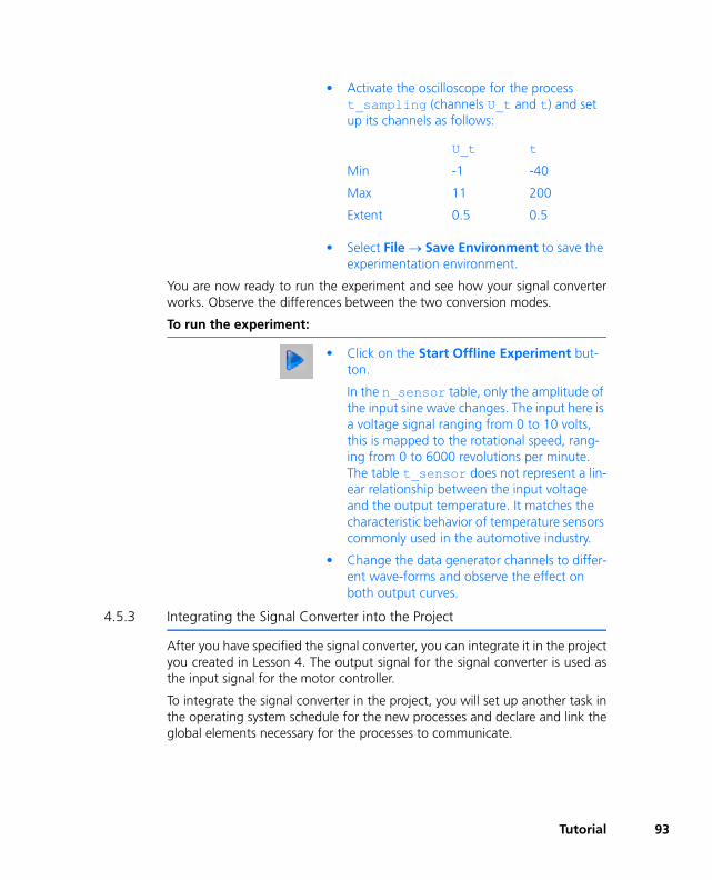
• Activate the oscilloscope for the process t_sampling (channels U_t and t) and set up its channels as follows:

• Select File → Save Environment to save the experimentation environment.

You are now ready to run the experiment and see how your signal converterworks. Observe the differences between the two conversion modes.

To run the experiment:

• Click on the Start Offline Experiment but-ton.

In the n_sensor table, only the amplitude of the input sine wave changes. The input here is a voltage signal ranging from 0 to 10 volts, this is mapped to the rotational speed, rang-ing from 0 to 6000 revolutions per minute. The table t_sensor does not represent a lin-ear relationship between the input voltage and the output temperature. It matches the characteristic behavior of temperature sensors commonly used in the automotive industry.

• Change the data generator channels to differ-ent wave-forms and observe the effect on both output curves.

4.5.3 Integrating the Signal Converter into the Project

After you have specified the signal converter, you can integrate it in the projectyou created in Lesson 4. The output signal for the signal converter is used asthe input signal for the motor controller.

To integrate the signal converter in the project, you will set up another task inthe operating system schedule for the new processes and declare and link theglobal elements necessary for the processes to communicate.

U_t t

Min -1 -40

Max 11 200

Extent 0.5 0.5

Tutorial 93

94

To add the signal converter to the project:

• Open the project editor for the project ControllerTest.

• Drag the module SignalConv from the "1 Database" list of the Component Manager to the "Outline" tab of the project.

• Click on the "OS" tab to activate the operat-ing system editor.

• Create a new task n_sampling.

• Set the period for the new task to 0.004 sec-onds.

• Assign the process n_sampling to the task n_sampling.

Tutorial

The project now has two tasks. The first task is activated every 10 milliseconds,the second one every 4 milliseconds. All the processes assigned to a given taskare executed at the interval specified. In the example, each task has only oneprocess, but it is possible to have any number of processes per task.

The next step in integrating the signal converter is to resolve communicationbetween the modules. Communication between the processes works throughglobal elements. All global elements used within a project have to be definedas messages in the corresponding modules.

By default, send messages are defined in a module while receive messages arenormally only imported into a module so they have to be defined now withinthe context of the project.

To set up the global elements:

• Select Extras → Global Elements → Resolve Globals to set up automatic links.

• Select Extras → Global Elements → Delete Unused Globals to remove the links from the previous lesson.

All the necessary global elements are created and linked automatically to thecorresponding elements with a matching name. The global message U_n, forinstance, is automatically linked to the message U_n in SignalConv.

Note that it is necessary to delete unused globals because the message n wasdefined in lesson 4 in the project context while it is now defined in the moduleSignalConv. The message n is now used for communication between theprocesses of the modules.

To experiment with the project:

• Select Build → Experiment to activate the experimentation environment.

• Open the event generator and enable the task n_sampling.

• Set the dT value for the task to 4 milliseconds.

During offline experimentation with projects, the event generator simulates the scheduling that is performed by the operating system during online experimentation.

• Open the data generator and delete the exist-ing data channel.

• Then set up a new channel for the message U_n.

Tutorial 95

96

• Set up the channel U_n as follows:

• Now activate U_n, the output voltage of the rotational speed sensor.

The signal converter converts the voltage value into the actual value for n using the characteristic table n_sensor.

The values given above produce an output range for n that matches the range from the previous experiment (without signal process-ing).


• Start the experiment.

The output curves should be the same as in the example without signal pro-cessing. The stimulus created by the data generator is different, but is thenprocessed in the table so that it looks the same as before.

4.5.4 Summary


• Creating and using characteristic fields

• Adding components to a project

• Define the communication between different components in a project

4.6 Modeling a Continuous Time System

The realistic modeling of physical, mechanical, electrical, and mechatronicalprocesses, often described by differential equations, requires continuous timemethods. Before integrating a method like this in the project created in theprevious chapters, this chapter covers modeling a time continuous systemusing a detailed example.

Mode: pulse

Frequency: 1.0 Hz

Phase: 0.0

Offset: 4/3

Amplitude: 1/3

Tutorial

ASCET supports the modeling and simulation of continuous time systems bymeans of so-called CT blocks. CT stands for "Continuous Time" and refers toitems that are modeled or calculated in quasi-continuous time intervals. Thecontinuous time modeling in ASCET is based on state space representation,the standard description form used in the design of continuous time systems.This representation allows the description of CT basic blocks by nonlinear ordi-nary first-order differential equations and nonlinear output equations. ASCETprovides several real-time integration methods to find optimal solutions tothese differential equations (refer to the ASCET online help for more informa-tion).

The procedure for modeling a continuous time system will now be explainedusing the example of a mass-spring pendulum with attenuation by the earth'sgravity.

4.6.1 Motion Equation

The mass m shown in the following illustration is subject to the followingforces:

• gravity: Fg = -mg(g = gravitational acceleration)

• Spring force: FF = - c (x + l0) (c = spring rate, l0 = length of spring at rest, and x = position of mass m)

• Attenuation FD = - d x’ (d = attenuation constant and x’ = velocity of mass)

This gives the motion equation as follows:

mx’’ = -mg + F or x’’ = -g + F/m (with F = FF + FD)

m

x

c

d

Tutorial 97

98

Breaking the second-order differential equation into two first-order differentialequations (x = x, v = x’) results in:

x’ = v

v’ = -g + F/m

These differential equations will be used in the following model design.

4.6.2 Model Design

For simplicity, the model of the mass-spring pendulum will be designed usinga single CT block. However, to illustrate the "direct pass-through" or "non-direct pass-through" properties and to demonstrate how to avoid an algebraicloop by skillful setting of these properties, we will design this model using twoblocks.

• The Force block calculates spring force F from the position of the pendulum’s mass m and the friction force from the velocity x’.

• From the spring force F the Mass block calculates the acceleration x’’ from the integration of which the velocity x’ and the position x result.

At first sight, this system looks like an algebraic loop: each block expects aninput value from the other block in order to calculate an output value requiredby the other block.

This algebraic loop can be avoided by clever setting of the direct pass-throughor non-direct pass-through properties:

• In the Force block, the output variable F via the equation

F = -c(x + l0) - dx’

is directly dependent on the input variables x and x’. This block is thus defined as having a direct pass-through.

• In the Mass block however, the output variables x and x’ do not depend directly on the input variable F, but on the internal state vari-ables of the block. These, at least at the start, have initial values from which the output variables x and x’ can be calculated, when the input variable F is unknown. Otherwise the output variables are calculated using the following differential equations:

x’ = v

Massx, x'

FForce

Tutorial

v’ = -g + F/m

This block is thus defined as having a non-direct pass-through.

Model Creation:

• In the Component Manager, create a folder and call it Lesson6.

• In this folder, use Insert → Continuous Time Block → ESDL to create a block Force and a block Mass.

• Double-click the Force block to open the ESDL editor.

• Click on the Input button to create two inputs x and v (type continuous).

• Click on the Output button to create an out-put F (type continuous).

• Click on the Parameter button to create the constants c (spring rate), d (attenuation con-stant) and l0 (length of the spring at rest).

The methods in the "Outline" tab are fixed by default.

Tutorial 99

100

• Right-click on each constant in the "Outline" tab in turn and select Data from the context menu.

The "Numeric Editor" dialog window opens.

• Assign realistic values to the constants (e.g., 5.0 to the spring rate c, 1.0 to the attenuation constant d, and 2.0 to the length of the spring at rest l0).

• In the "Outline" tab, click on the method directOutputs[].

• In the "Edit" field, specify the formula used to calculate the force:

F = -c * (x + l0) - d*v;

• Click on the Generate Code button.

The CT block Force is compiled.

• Double-click the Mass block to open the ESDL editor.

• As above, create an input F, two outputs x and v, one parameter m (mass), and one con-stant g (gravitational acceleration).

• Assign values to g and m as described above (9.81 to g and, e.g., 2.0 to the mass m).

Tutorial

• Click on the Continuous State button to cre-ate state variables x_local and v_local for the internal calculation of the outputs.

• For the derivatives[] method, specify the differential equations required for the cal-culation:

x_local.ddt(v_local);

v_local.ddt(-g + F/m);

• In nondirectOutputs[] pass the state variables x_local and v_local to the out-puts x and v:

x=x_local;

v=v_local;

• In the init[] method, you can provide the system with realistic initial values for x and v using the resetContinuousState() func-tion.

resetContinuousState(x_local,0.0);

resetContinuousState(v_local,0.0);

• Click on the Generate Code button.

The CT block Mass is compiled.

The combination of the two basic CT blocks into one CT structure block isdone using the Block Diagram Editor (BDE).

Tutorial 101

102

To combine the two basic CT blocks.

• In the Component Manager, Lesson6 folder, select Insert → Continuous Time Block → Block Diagram to create a new block Mass_Spring.

• Double-click the new block to open it in the Block Diagram Editor.

• In the Component Manager, drag and drop the Mass and Force blocks (one at a time) to the BDE window and file them.

• Connect the corresponding inputs and out-puts with each other.

• Select Build → Experiment.

The CT block is now compiled, and the exper-iment is started.

Note

Double-clicking one of the CT basic blocks makes it available for editing. Note, however, that any modification to the blocks affects the entire library, i.e., all structure blocks that use these basic blocks.

Tutorial

• Create the experimentation environment required with numeric editors for the parame-ters and graphical displays.

• Scale the channels in the oscilloscope sepa-rately, from -10 to 0 for x, from -8 to +8 for v.

4.6.3 Summary

After finishing this lesson, you should be able to carry out the following tasksin ASCET:

• Creating a model to simulate a process

• Using the ESDL editor to create CT blocks with direct and non-direct pass-through

• Using the Block Diagram Editor to combine CT blocks

• Performing the physical experiment

Tutorial 103

104

4.7 A Process Model

Following the introduction of CT blocks in the last chapter, you will now usethem for testing your controller. In ASCET you can develop a model of thetechnical process to be controlled, and then experiment with a closed controlloop. This means that way the controller can be thoroughly tested before it isused in a real vehicle.

In our example here, the motor is the technical process. It returns a value U_nwhich is a sensor reading of the rotational speed of the engine. This value isprocessed by the controller, which returns a value air_nominal. The control-ler output value determines the throttle- position of the engine, and thus inturn influences the rotational speed.

Fig. 4-1 A closed-loop experiment

You will use a CT block for this process model. This type of component is par-ticularly suitable for process models. The model is based on the following dif-ferential equation, which models a PT2 - system:

T2 s’’ + 2DTs’ + s = Ku

Equ. 4-1 A PT2 - system

The parameters T, D and K have to be set up with appropriate values.

4.7.1 Specifying the Process Model

Creating continuous time components is different from creating other compo-nents. They have inputs and outputs which are the equivalent of argumentsand return values. The main difference is that a continuous time block canhave multiple inputs and outputs which are not tied to a particular method.There is a fixed set of methods defined in each continuous time block, thatcannot be modified by the user.

Controller

Technical Process

U_n

air_nominal

Tutorial

You will use ESDL Code for the example here. The syntax of the ESDL code issimilar to C++ or Java. An object method is called with the name of the object,a dot, the name of the method and the arguments in brackets followed by asemicolon. The method used for deriving is called ddt(). For example, theequation is equivalent to the ESDL statement s.ddt(sp);.

To create a continuous time component:

• In the Component Manager create the folder Tutorial\Lesson7.

• To add a continuous time block, select Insert → Continuous Time Block → ESDL.

• Name the new component ProcModel.

• Select Edit → Open Component to open the ESDL editor.

You can, of course, also use the external text editor. There are instructions for this in the first part of the tutorial.

To edit the process model, first add the elements required and then edit themethods derivatives and non directOutput.

To edit the process model:

• In the ESDL editor, use the Continuous State button to create two continuous states.

• Name the states s and sp.

• Create an input u.

• Create an output y.

Both elements are of type cont.

sp s·=

Tutorial 105

106

• Create the parameters D, K and T.

The "Outline" tab for the process model should look like this:

• Adjust the parameters as follows:

D = 0.4,

K = 0.002,

T = 0.05.

• In the "Outline" tab, select the deriva-tives method and edit the code as follows:

s.ddt(sp);

sp.ddt((K*u-2*D*T*sp-s)/(T*T));

• Select the nondirectOutputs method and type in the following text.

y = s;

• Adjust the layout in the layout editor.

Note that in a process model it is preferable to put the outputs on the left and the inputs on the right.

Note

See the ASCET online help for specifying CT blocks for information on how to resolve a differential equation.

Tutorial

• Select Edit → Save.

• In the Component Manager, click on the Save button to save the process model.

You can now start experimenting with the new model.

To experiment with the model:

• In the ESDL editor, select Build → Experi-ment to open the experimentation environ-ment.

• Click on the Open CT Solver button to open the "Solver Configuration" dialog pane.

The configuration is displayed as follows:

• Click OK to accept the default configuration.

• Open the data generator and create a channel for the input u.

• Set up the channel u with the following val-ues:

• Open an oscilloscope window with the chan-nels u and y.

Mode: pulse

Frequency: 0.5 Hz

Phase: 0.0 s

Offset: -0.5

Amplitude: 1.0

Tutorial 107

108

• Set the Measure Channels for the oscilloscope as follows:


• Start the experiment.

The output should look like this:

4.7.2 Integrating the Process Model

To create a closed control loop, we will now integrate the process model intothe controller project we created earlier. The steps required are the same asbefore: including the module, setting up the operating system and linking theglobal elements.

u y

Min -1 -0.002

Max 2 0.004

Extent 3.0 3.0

Note

The process model is added to the same project for simplicity. This is often useful in the early stages of testing closed loop simulation. In regular projects, the process model would be distributed over a network in another project since they are not part of the same embedded system.

Tutorial

To include the process model:

• From the Component Manager, open the project editor for ControllerTest.

• In the project editor, add the component ProcModel to the "Outline" tab.

• Activate the "OS" tab of the project editor to specify the scheduling for the CT tasks.

• Select the task simulate_CT1 and set the value in the "Period" field to 0.01 s.

The controller and the process model both run in the same time interval.

Linking the continuous time blocks and the modules cannot be done automat-ically. They have to be connected explicitly in a block diagram.

To adjust the linking between modules and CT block:

• Click the "Graphics" tab.

• From the "Outline" tab, drag the three com-ponents and drop them into the drawing area.

• Connect the messages of the modules with the corresponding input and output of the CT block.

To construct the example, connect the output y of ProcModel with the global message U_n and connect the input u of ProcModel with the global message air_nominal.

Tutorial 109

110

• Right-click on each component and select Unconnected Ports to remove these ports from the diagram.

Linking the messages for communicating between modules is done automati-cally. Messages that have the same name are linked with each other.

The project is now complete and ready for experimentation. We will nowexperiment online, which requires an ASCET-RP installation and a real-time tar-get (e.g. ES1000). If you do not have both, you will have to continue by exper-imenting offline as before.

To set up the project for online experimentation:

• Click on the Project Propertiesbutton.

Note

If you continue by experimenting offline, be sure to remove the global mes-sage U_n from the data generator.

Tutorial

• In the "Project Properties" dialog window, "Build" node, select the target ES1130 and the GNU-C V3.4.4 (Power-PC) compiler.

These options specify the hardware and the corresponding compiler for code generation.

• Click OK to close the "Project Properties" dia-log window.

The buttons Reconnect to Experiment of selected Experiment Target and Select Hardware are now available.

• Click on the "OS" tab to activate the operat-ing system editor.

• To copy the schedule you created earlier, select Operating System → Copy From Target.

• From the "Selection Required" dialog, select PC and click OK.

The project for the new target now has the same scheduling as that specified before for the offline PC simulation.

Tutorial 111

112

There are several differences from the offline experiment. In the online experi-ment, there is no event or data generator. The event generator serves to simu-late the scheduling of the operating system tasks generated for onlineexperiments.

In the online experiment the experimentation code and the measurements arestarted separately, and have separate buttons in the toolbar. This is because themeasurements may influence the real-time behavior of the experiment, so itmay sometimes be necessary to switch them off.

To experiment with the project online:

• Select Online (RP) from the "Experiment Target" combo box.

Offline (RP) is intended for offline exper-iments on the target.


The code for the experiment is generated and the experiment opens with the same environ-ment as defined previously.

Tutorial

If your project contains several tasks, you could well be prompted to select one acquisi-tion task for each measure value.

• In the "Selection Required" window, select the #3 simulate_CT1 task and click OK.

• Include n and n_nominal in the existing oscilloscope and set their value range from 0 to 2000.

• Open numeric editors for the variables n_nominal, Ki and Kp.

• Click on the Start OS button and then click on the Start Measurement button.

The experiment starts and the results are dis-played on the oscilloscope. The value for n should quickly approach n_nominal and stay there.

• Modify n_nominal in the numeric editor.

The value n should change in line with all the changes to n_nominal.

• You can optimize the behavior of the control loop by adjusting the Ki and Kp parameters.

4.7.3 Summary


• Creating and specifying continuous time blocks

• Experimenting with continuous time blocks

• Integrating continuous time blocks in a project

Start OS

Start Measurement

Tutorial 113

114

• Creating variable links

• Switching between different targets

• Experimenting online with a project

4.8 State Machines

State machines are useful for modeling systems that move between a limitednumber of distinct states. ASCET provides a powerful mechanism for specify-ing components as state machines. In this lesson we will specify and test asimple state machine that implements a temperature dependent change in thenominal number of revolutions of an idling engine. That state machine willthen be integrated into our project. In the next chapter we will then constructhierarchical state machines.

If the engine is cold, it has to idle at a higher speed to keep it turning over.Once the engine has warmed up, the rotational speed for idling can bedecreased to reduce fuel consumption. Our state machine thus has two states:one when the engine is cold, and one when it is warm. It represents a two-phase control.

4.8.1 Specifying the State Machine

A state machine consists of the state graph itself and a number of specifica-tions of actions and conditions. The actions and conditions can be specifiedusing either block diagrams or ESDL code. They determine what happens inthe various states and during the transitions between states.

The diagrams are specified in the block diagram editor. Another possibility is towrite ESDL code directly in a text editor which can be opened for every stateand every transition (i.e., without opening the ESDL editor). State machineshave inputs and outputs for data transfer with other components.

To create a state machine:

• In the Component Manager, create the folder Tutorial\Lesson8.

• Select Insert → State Machine or click on the Statemachine button to create a new state machine.

• Name it WarmUp.

Tutorial

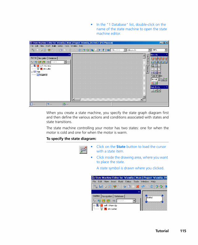
• In the "1 Database" list, double-click on the name of the state machine to open the state machine editor.

When you create a state machine, you specify the state graph diagram firstand then define the various actions and conditions associated with states andstate transitions.

The state machine controlling your motor has two states: one for when themotor is cold and one for when the motor is warm.

To specify the state diagram:

• Click on the State button to load the cursor with a state item.

• Click inside the drawing area, where you want to place the state.

A state symbol is drawn where you clicked.

Tutorial 115

116

• Create a second state symbol and place it below the first one in the drawing area.

• Right-click on the state symbol you created first and select Edit State from the context menu to open the State Editor.

• In the "State" field, enter the name coldEngine.

• Activate the Start State option to determine the state the machine is in when it is first started.

There must be start state for each state machine.

• Click on OK to close the State Editor.

The name is displayed in the state symbol.

• Name the second state symbol warmEngine.

• Right-click in the drawing area, outside any symbol, to activate the connection mode.

Tutorial

• Click in the right half of the coldEngine state symbol to begin a connection, then click in the right half of the warmEngine state symbol to connect the two states.

A line is drawn between the two state sym-bols. It has an arrow at one end, pointing from the top to the bottom symbol. The lines repre-sent possible transitions between states.

• Create another transition from left half of the bottom to the left half of the top symbol.

• Select File → Save to store the diagram.

• In the Component Manager, select File → Save Database to save the database.

The next step in building the state machine is to specify its interface. You needan input for the temperature value and an output for the number of revolu-tions. In addition, parameters are required that specify high and low tempera-ture and number of revolutions per minute.

To specify the interface of the state machine:

• Create an input by clicking the Input button.

• Name the input t.

• Create an output by clicking on the Output button.

• Name the output n_nominal.

• Use the Continuous Parameter button to create four parameters.

Tutorial 117

118

• Name the parameters and set their values as follows:

t_up = 70

t_down = 60

n_cold = 900

n_warm = 600

You can now proceed by specifying the actions and conditions for both thestates and the transitions between states. You can specify three actions foreach state:

• The entry action is executed each time the state is entered.

• The exit action is executed each time the state is left.

• The static action is executed while the state machine remains station-ary.

Similarly, a trigger event, a condition, a priority and an action can be specifiedfor each transition. The name of the trigger and of the condition appear nextto the transition. One trigger is automatically created when the state machineis created.

The actions and conditions are specified in ordinary diagrams or in ESDL code.In this example you will use ESDL code.

To specify the trigger actions and conditions:

• Right-click on the transition from the cold-Engine state to warmEngine.

• From the context menu, select Edit Transi-tion to open the Transition Editor.

The condition for a transition from cold to warm is that the actual temperature value t is greater than t_up.

• On the "Condition" tab, select <ESDL> from the combo box.

Note that you can influence the predefined choice of options in this combo box.

Tutorial

• Enter the code shown below in the code pane of the condition:

If the condition evaluates to true, the idle speed of the engine is set to n_warm.

Note that this code is displayed in the state machine diagram. In this example, an alias name is created for the transition condition and shown in the diagram.

• Select <ESDL> for the action, too, and enter the following code:

n_nominal = n_warm;

• Click OK to close the Transition Editor.

• Look at the diagram. Note that the condition and the action from the state machine can be seen.

• Open another editor for the transition from warmEngine to coldEngine.

• Select <ESDL> for the condition and enter the following code:

Note

In the Transition Editor, the condition is not ter-minated with a semicolon. This is also true for regular ESDL code where conditions appear in parentheses.

Tutorial 119

120

t < t_down

Note that this time the complete code is shown in the diagram as no alias was assigned (in a comment).

• Select <ESDL> for the action, too, and enter the following code:

n_nominal = n_cold;

• Close the transition editor and select File → Save.

You can also specify the actions and conditions as block diagrams instead ofESDL code. For that purpose, you first create a separate diagram for actionsand conditions.

To create a diagram for actions/conditions:

• In the state machine editor, select Insert → Diagram → Actions/Conditions BDE.

A diagram named ActionCondition_BDE is created in the "Outline" tab.

• Accept the default name.

Now you can add, and specify, actions and conditions.

To specify the action/condition as block diagram:

• In the "Diagrams" field, click on the Action-Condition diagram.

Tutorial

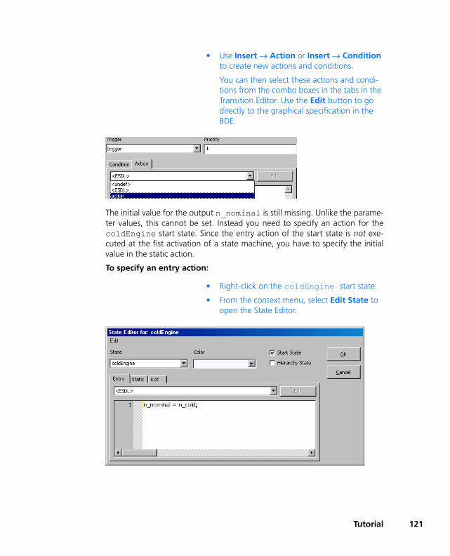
• Use Insert → Action or Insert → Condition to create new actions and conditions.

You can then select these actions and condi-tions from the combo boxes in the tabs in the Transition Editor. Use the Edit button to go directly to the graphical specification in the BDE.

The initial value for the output n_nominal is still missing. Unlike the parame-ter values, this cannot be set. Instead you need to specify an action for thecoldEngine start state. Since the entry action of the start state is not exe-cuted at the fist activation of a state machine, you have to specify the initialvalue in the static action.

To specify an entry action:

• Right-click on the coldEngine start state.

• From the context menu, select Edit State to open the State Editor.

Tutorial 121

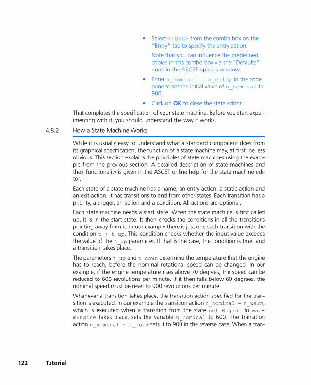
122

• Select <ESDL> from the combo box on the "Entry" tab to specify the entry action.

Note that you can influence the predefined choice in this combo box via the "Defaults" node in the ASCET options window.

• Enter n_nominal = n_cold; in the code pane to set the initial value of n_nominal to 900.

• Click on OK to close the state editor.

That completes the specification of your state machine. Before you start exper-imenting with it, you should understand the way it works.

4.8.2 How a State Machine Works

While it is usually easy to understand what a standard component does fromits graphical specification, the function of a state machine may, at first, be lessobvious. This section explains the principles of state machines using the exam-ple from the previous section. A detailed description of state machines andtheir functionality is given in the ASCET online help for the state machine edi-tor.

Each state of a state machine has a name, an entry action, a static action andan exit action. It has transitions to and from other states. Each transition has apriority, a trigger, an action and a condition. All actions are optional.

Each state machine needs a start state. When the state machine is first calledup, it is in the start state. It then checks the conditions in all the transitionspointing away from it. In our example there is just one such transition with thecondition t > t_up. This condition checks whether the input value exceedsthe value of the t_up parameter. If that is the case, the condition is true, anda transition takes place.

The parameters t_up and t_down determine the temperature that the enginehas to reach, before the nominal rotational speed can be changed. In ourexample, if the engine temperature rises above 70 degrees, the speed can bereduced to 600 revolutions per minute. If it then falls below 60 degrees, thenominal speed must be reset to 900 revolutions per minute.

Whenever a transition takes place, the transition action specified for the tran-sition is executed. In our example the transition action n_nominal = n_warm,which is executed when a transition from the state coldEngine to war-mEngine takes place, sets the variable n_nominal to 600. The transitionaction n_nominal = n_cold sets it to 900 in the reverse case. When a tran-

Tutorial

sition occurs, the state machine also executes the exit action of the state itleaves, and the entry action of the state it enters. In our example, these areempty and nothing happens.

Once the state machine has entered the second state, it stays in that state untilthe condition in the transition from the second to the first state is fulfilled.While the state machine stays in one state, the static action is executed everytime the state machine is triggered. Triggering is always an outside event whichstarts one pass through the state machine.

A pass through a state machine consists of first testing all the conditions ontransitions leading away from the current state. Transitions and their condi-tions are tested in order of their priorities. If a condition is true, the correspond-ing transition is performed and the exit, transition and entry actions areexecuted. Once the first condition checks out true, any other transitions lead-ing from the same state but having lower priorities are not tested. If no condi-tion is true, the machine remains in the current state and performs the staticaction once for each pass.

Once the condition in the second transition of our state machine is true, i.e. ifthe input value falls below the threshold, the state machine returns to the firststate. The machine then remains in that state (doing nothing, because there isno static action) until the input value grows larger than the threshold again.

4.8.3 Experimenting with the State Machine

The experimentation environment works the same for state machines as forother types of components. One extra feature for experimenting with statemachines is their animation, i.e. the current state is highlighted in the statemachine diagram while the experiment is running.

Tutorial 123

124

To experiment with the state machine:

• In the state machine editor, select Build → Experiment to open the experimentation environment.

• Right-click on one of the states and select Animate States from the context menu.

• Enable the trigger event.

• In the data generator, create a channel for the variable t.

• Assign a sine-wave with frequency 1 Hz, off-set 70, and amplitude 20 to the channel.

• Open an oscilloscope window for t and n_nominal.

• Click on the Start Offline Experiment but-ton to experiment with the state machine.

• Change the colors of the individual states to improve clarity.

• To do this, use the Exit to Component but-ton to leave the experimentation environ-ment, and call the state editor.

Tutorial

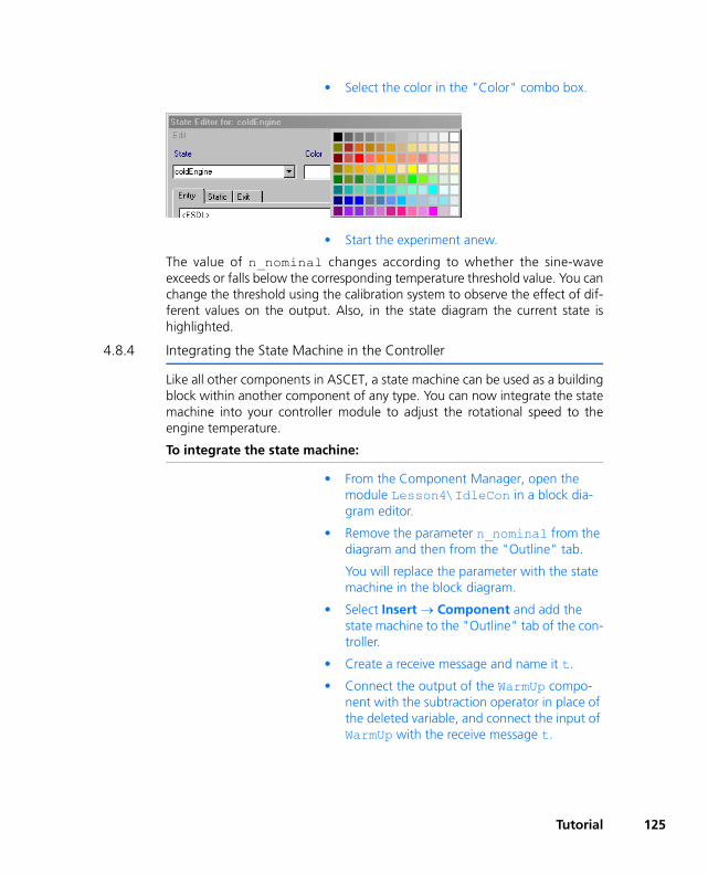
• Select the color in the "Color" combo box.

• Start the experiment anew.

The value of n_nominal changes according to whether the sine-waveexceeds or falls below the corresponding temperature threshold value. You canchange the threshold using the calibration system to observe the effect of dif-ferent values on the output. Also, in the state diagram the current state ishighlighted.

4.8.4 Integrating the State Machine in the Controller

Like all other components in ASCET, a state machine can be used as a buildingblock within another component of any type. You can now integrate the statemachine into your controller module to adjust the rotational speed to theengine temperature.

To integrate the state machine:

• From the Component Manager, open the module Lesson4\IdleCon in a block dia-gram editor.

• Remove the parameter n_nominal from the diagram and then from the "Outline" tab.

You will replace the parameter with the state machine in the block diagram.

• Select Insert → Component and add the state machine to the "Outline" tab of the con-troller.

• Create a receive message and name it t.

• Connect the output of the WarmUp compo-nent with the subtraction operator in place of the deleted variable, and connect the input of WarmUp with the receive message t.

Tutorial 125

126

• Adjust the diagram as shown below. Be sure to adjust the sequencing in the diagram to include all items in the correct order.

• Save the diagram and click on the Save but-ton in the Component Manager.

In order to make the modified controller work with our project, we have tomake some adjustments to the project. At this point we will also integrate thetemperature sensor, which has been left unused so far.

To modify the project:

• Open the project editor for the project Con-trollerTest.

• Switch to the "OS" tab.

• Assign the process t_sampling to the task Task10ms.

• Use the command Task → Move Up to make the process t_sampling the first in that task.


• Open an additional scalar calibration window for the value U_t.

• Add the variable t to the oscilloscope.

• Click on the Start OS button.

• Click on the Start Measurement button.

• Adjust the value U_t and observe its effect.

If the value of t exceeds the 70 degree limit, the state machine switches to nominal value for n to the lower value of 600. If the temper-

Start OS

Start Measurement

Tutorial

ature falls to below 60 degrees (simulated by adjusting U_t), the nominal value for n regains the original value of 900.

4.8.5 Summary


• Creating a state diagram

• Creating and assigning conditions, actions and triggers

• Experimenting with state machines

• Integrating state machines into other components

4.9 Hierarchical State Machines

Now that you have familiarized yourself with the way state machines work inthe preceding lesson, we shall look at creating a more complex system. Thisunit concentrates on hierarchical state machines. You will also learn how touse the system libraries and components supplied with ASCET, such as timers.

ASCET permits structuring of state machines in closed and open hierarchies.With closed hierarchies, the internal functionality is concealed, with open hier-archies the substates are also shown graphically.

You will build a traffic light control system to run through the individual phasesof a traffic light using parameterizable timing. The traffic light will also have anerror status where it will flash.

4.9.1 Specifying the State Machine

First you will import the libraries you need and prepare for the task.

To import the system library:

• In the Component Manager, click on Import.

The "Select Import File" window opens.

• In the "Import File" field, use the button to select the file SystemLibETAS.exp from the Export directory of your ASCET installation (e.g. C:\etas\ASCET6.0\export).

The OK button is now available.

Tutorial 127

128

• Click OK to start the import.

The "Import" window opens. All objects con-tained in the file are selected.

• Confirm the import of all files with OK.

The files are imported. This can take up to sev-eral minutes. When the import procedure is finished, all imported items are listed in the "Imported Items" window.

The second step is to specify the two main states possible for the traffic light(NormalMode and ErrorMode).

To create the state machine:

• In the Component Manager, create the folder Tutorial\Lesson9.

• Select Insert → State Machine to create a new state machine, and call it Light.

• Select Edit → Open Component to open the state machine editor.

You can start specifying the state machine that will control your traffic light.

• Create the two states ErrorMode and NormalMode.

Then add a timer to your project from the system library.

To add the timer object:

• Select Insert → Component.

• In the "Select Item" dialog, select the timer object Timer from the Counter_Timer folder of the SystemLib_ETAS library.

• Confirm your selection with Ok.

You have now added an object Timer to the "Outline" tab for your state machine.

To specify the state diagram:

• Specify the necessary data elements as fol-lows:

– An input error of type Logic,

Tutorial

– three outputs (yellow, green, red) of type Logic to symbolize traffic light col-ors,

– four continuous parameters (Blink-Time, YellowTime, GreenTime, RedTime) for the different traffic light phases.

To get more practice with dependent parame-ters, you will configure the parameters so that only the green phase is specified; the other parameters are given values dependent on that:

RedTime = 2 * GreenTime

YellowTime = GreenTime/3

BlinkTime = YellowTime/10

• Now specify calculations and dependencies of the individual parameters.

• To do this, activate the Dependent option under "Dependency" in the properties editor for the parameters RedTime, YellowTime and BlinkTime.

The properties editor is started with a double-click on the element name or via the Edit con-text menu.

• Click on the Formula button to start the for-mula editor.

• Using the formula editor, specify the calcula-tion for each of the dependent parameters by first creating a formal parameter x and then entering the calculation in the formula pane.

Redtime : 2*x

YellowTime : x/3

BlinkTime : x/10

• Close the formula editor and the properties editor.

• Open the dependency editor via the context menu Edit Data.

Tutorial 129

130

• Assign the corresponding model parameter to the formal parameter x for each of the depen-dent parameters.

RedTime : x = GreenTime

YellowTime : x = GreenTime

BlinkTime : x = YellowTime

• Give the data elements meaningful values (e.g. GreenTime = 5).

• Open the state editor for the ErrorMode state.

You can open the state editor either by dou-bleclicking on a state or via the Edit State context menu.

• Define this state as the initial state and color it red.

• Enlarge both states so that the hierarchies can be inserted.

• Create the transitions between the two states.

• Open the transition editor via the Edit Transi-tion context menu or with a double-click on the graphic.

• Specify the transitions between the two states by entering conditions in the transition dialog. Enter the conditions in ESDL so that the nor-mal state NormalMode is activated when the

Tutorial

input error is false (i.e. there has not been an error), and ErrorMode is activated when there is an error.

• Select File → Save.

• Save your work in the Component Manager by selecting File → Save Database.

• You might like to experiment with the main states.

The next step towards creating the traffic light control system is to specify thesubstates. First specify the performance in the error mode (state ErrorMode).In this state, a yellow flashing light will be output. To do this, introduce twosubstates YellowOff and YellowOn; with the timer as switch betweenthem. In the YellowOn state, the output yellow will be set to true, whilethe YellowOff state sets it back to false.

To specify the substates for the error mode

• Create the states YellowOff and Yel-lowOn and place them inside the state ErrorMode.

Tutorial 131

132

• Define YellowOff as start state and color YellowOn yellow.

• Define the response of the state YellowOff in the state editor.

To do this, call the state editor either via the Edit State context menu or with a double-click on the state.

• For the entry action, select ESDL in the combo box for the "Entry" tab and enter the follow-ing code:

green = false;

red = false;

yellow = false;

Timer.start(BlinkTime);

• For the static action, enter the following code on the "Static" tab:

Timer.compute();

• Now define and describe the YellowOn state in the same way.

Entry action:

yellow = true;Timer.start (BlinkTime);

Static action:

Timer.compute();

Tutorial

• Now define the transitions between the two substates.

The condition for a state transition is that the timer has run out (Timer.out() == false).

This means that the ErrorMode state is started in the YellowOff state. Aswell as switching off the color signals, the entry action starts the timer with theparameterizable flashing time. The static action of the YellowOff state callsthe timer function compute() each time, which decrements the timercounter. When this counter is 0, the timer function out() returns the codefalse, thus fulfilling the transition condition. The state YellowOn works ina similar way, however, in the entry action, the Yellow color signal is switchedon.

The next step is to specify the performance in normal operation. To do this,create a start state, AllOff, and place it within the NormalMode state. Usethe exit action to set all the color signals to a defined state. Now think about asuitable response for the traffic light control system.

In this example, you should describe the activation or deactivation of the indi-vidual color signals in the transition actions, not in the entry actions of thestates.

To specify the substates in normal operation

• Create the states AllOff (start state), Yel-low, Red, RedYellow and Green and place them inside the NormalMode state..

Tutorial 133

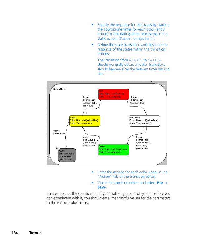
134

• Specify the response for the states by starting the appropriate timer for each color (entry action) and initiating timer processing in the static action. (Timer.compute()).

• Define the state transitions and describe the response of the states within the transition actions.

The transition from AllOff to Yellow should generally occur, all other transitions should happen after the relevant timer has run out.

• Enter the actions for each color signal in the "Action" tab of the transition editor.

• Close the transition editor and select File → Save.

That completes the specification of your traffic light control system. Before youcan experiment with it, you should enter meaningful values for the parametersin the various color timers.

Tutorial

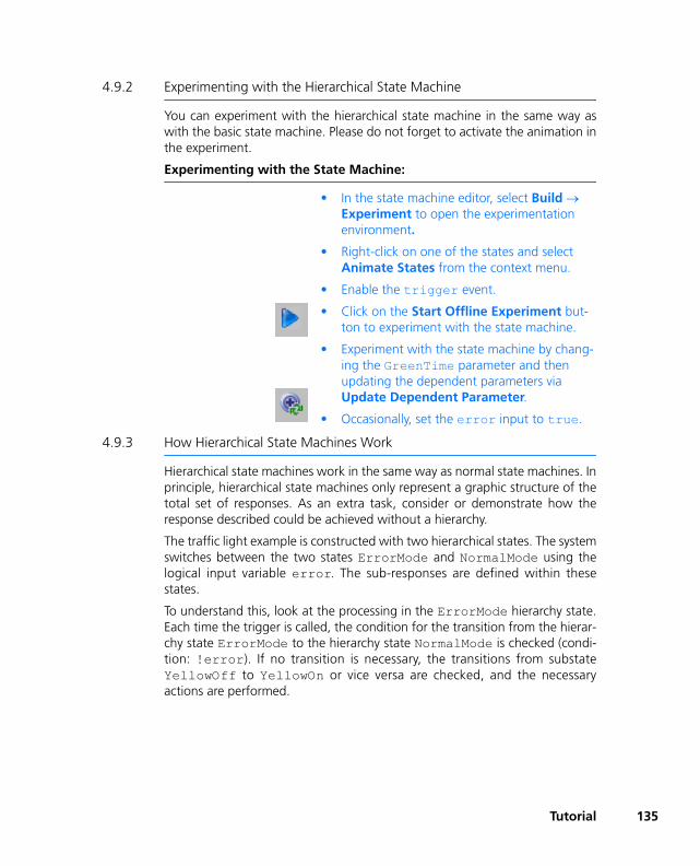
4.9.2 Experimenting with the Hierarchical State Machine

You can experiment with the hierarchical state machine in the same way aswith the basic state machine. Please do not forget to activate the animation inthe experiment.

Experimenting with the State Machine:

• In the state machine editor, select Build → Experiment to open the experimentation environment.

• Right-click on one of the states and select Animate States from the context menu.

• Enable the trigger event.

• Click on the Start Offline Experiment but-ton to experiment with the state machine.

• Experiment with the state machine by chang-ing the GreenTime parameter and then updating the dependent parameters via Update Dependent Parameter.

• Occasionally, set the error input to true.

4.9.3 How Hierarchical State Machines Work

Hierarchical state machines work in the same way as normal state machines. Inprinciple, hierarchical state machines only represent a graphic structure of thetotal set of responses. As an extra task, consider or demonstrate how theresponse described could be achieved without a hierarchy.

The traffic light example is constructed with two hierarchical states. The systemswitches between the two states ErrorMode and NormalMode using thelogical input variable error. The sub-responses are defined within thesestates.

To understand this, look at the processing in the ErrorMode hierarchy state.Each time the trigger is called, the condition for the transition from the hierar-chy state ErrorMode to the hierarchy state NormalMode is checked (condi-tion: !error). If no transition is necessary, the transitions from substateYellowOff to YellowOn or vice versa are checked, and the necessaryactions are performed.

Tutorial 135

136

If you now look at NormalMode, this means that, again, for each trigger callit is first checked whether the input error is true, and therefore a transitionto ErrorMode is necessary. Only if this is not the case, the transitions from thesubstates (AllOff, Yellow, Red, RedYellow, Green) are checked. In thetraffic light example, it is checked whether the timer has run out.

You can have a look at the code generated from the state diagram to clarifythis process.

Displaying generated code:

• In the state machine editor, select Build → View Generated Code to display the code generated.

The code from the components is written to a temporary file and then opened with an appli-cation defined in the operating system register database.

4.9.4 Summary


• Create hierarchical state diagrams

• Describe the way the states behave in actions and also in the transition actions.

• Import modules, classes or components

• Import system components from ASCET libraries

• Use the Timer system component

• Use of dependent parameters

• Displaying generated code

Note

In order to display the code generated, a search is made in the operating system register data-base for an application with associated files of type *.c and *.h. Depending on the file end-ings registered, the relevant editor is started.

Tutorial

5 Glossary

In this glossary the technical terms and abbreviations used in the ASCET docu-mentation are explained. Many terms are also used in a more general sense,but only the meaning specific to ASCET is explained here.

The terms are listed in alphabetic order.

5.1 Abbreviations

ASAM-MCD

Association for Standardisation of Automation- and Measuring Sys-tems, with the working groups Measuring, Calibration, Diagnosis (German: Arbeitskreis zur Standardisierung von Automations- und Messsystemen, mit den Arbeitsgruppen Messen, Calibrieren und Diag-nose)

ASCET

Development tool for control unit software

ASCET-MD

ASCET Modeling and Design

ASCET-RP

ASCET Rapid Prototyping

ASCET-SE

ASCET Software Engineering

AUTOSAR

Automotive Open System Architecture; see http://www.autosar.org/

BDE

Block Diagram Editor

CPU

Central Processing Unit

ECU

Embedded Control Unit

ERCOSEK

ETAS real-time operating system, OSEK-compliant

ESDL

Embedded Software Description Language

Glossary 137

http://www.autosar.org/

138

ETK

emulator test probe (German: Emulatortastkopf)

FPU

Floating Point Unit

HTML

Hypertext Markup Language

INCA

Integrated Calibration and Acquisition Systems

INTECRIO

A new ETAS product family. INTECRIO integrates code from various behavioral modeling tools, facilitates all necessary configurations, allows the generation of executable code, and provides an experiment environment for the execution of the Rapid Prototyping experiment.

OS

Operating System

OSEK

Working group "open systems for electronics in automobiles"(German: Arbeitskreis Offene Systeme für die Elektronik im Kraftfahr-zeug)

RAM

Random Access Memory

RE

Runnable entity; a a piece of code in an SWC that is triggered by the RTE at runtime. It corresponds largely to the processes known in ASCET.

ROM

Read-Only Memory

RTA-RTE

AUTOSAR runtime environment by ETAS

RTE

AUTOSAR runtime environment; provides the interface between soft-ware components, basic software, and operating systems.

SWC

Atomic AUTOSAR software component; the smallest non-dividable software unit in AUTOSAR.

Glossary

UML

Unified Modeling Language

XML

Extensible Markup Language

5.2 Terms

Action

An action is part of a state machine and associated with states or tran-sitions of the state machine. An action is a piece of functionality, whose execution is triggered by the state machine.

Application Modes

An application mode is part of the operating system of ASCET. An operating mode describes different conditions a system can be in, e.g. EEPROM-programming mode, warm-up, or normal mode.

Argument

An argument is the input to a method of a class. Arguments can only be used in the specification of the method they belong to, and not in other methods of the class.

Arithmetic Services

User-defined C functions to optimize elementary operations, such as addition operations, and to extend such operations with special prop-erties, such as value limits.

Array

An array is a one dimensional static list of elements of the basic scalar type continuous or discrete, indexed by the basic scalar type discrete.

ASAM-MCD-2MC file

Default exchange format used for projects in ASCII format for the description of measurement and calibration values. The files have the extension *.a2l.

Basic Model Types

Basic model types are used to model physical behavior. There are three types: continuous, discrete and logical. A number of opera-tions, such as addition or comparison, are defined for the basic model types. The implementation is used to transform the model types to implementation types.

Glossary 139

140

Block Diagram

A block diagram is a graphical description for a component in which the various elements, operators and inputs/arguments and outputs/return values are connected by directed lines. A block diagram consists of several diagrams. The description in terms of block diagrams is a physical description in contrast to the description with C-Code.

Bypass Experiment

In a bypass experiment, ASCET is directly connected to a microcontrol-ler, and parts of the microcontroller software are simulated by ASCET.

Calibration

Calibration is the manipulation of the values (physical / implementa-tion) of elements during the execution of an ASCET model (experi-ment).

Calibration Window

ASCET working window which can be used to modify parameters.

C Code

C code is an implementation dependent description of a component.

Characteristic

General term used for characteristic map, curve and value (see also "Parameter".

Characteristic Line

Two-dimensional parameter.

Characteristic Map

Three-dimensional parameter.

Characteristic value

One-dimensional parameter (constant).

Class

A class is one of the component types in ASCET. Classes in ASCET are like object-oriented classes. The functionality of a class is described by methods.

Code

The executable code is the "actual" program with the exception of the data (contains the actual algorithms). The code is the program part which can be executed by the CPU.

Glossary

Code Generation

Code generation is the first step in the transformation of a physical model to executable code. The physical model is transformed into ANSI C-Code. Since the C-Code is compiler (and therefore target) depen-dent, different code for each target is produced.

Component

A component is the basic unit of reusable functionality in ASCET. Com-ponents can be specified as classes, modules, or state machines. Each component is built up of elements which are combined with operators to build up the functionality.

Component Manager

Working environment in which the user can set up ASCET and manage the data he created and which are stored in the database.

Condition

A condition is used to describe the control flow in a state machine. It returns a logical value which determines, whether a transition from one state to another takes place.

Configuration dialog box

Dialog box used to configure the individual measuring and calibration windows as well as the variables contained therein.

Constant

A constant is an element that cannot be changed during execution of an ASCET model.

Container

Containers serve as containers for projects, classes and modules. Their purpose is to structure models and databases and place different data-base items under a common version control.

Data

The data is the variables of a program used for calibration.

Data Generator

The data generator is part of the experimentation environment. It is used to stimulate the inputs or variables in the model under experimen-tation.

Data Logger

With the data logger measurement data can be read from an experi-ment and stored to disk for further analysis.

Glossary 141

142

Data Set

A data set contains/references the initial data for all elements of a com-ponent or project.

Database

All information specified or produced with ASCET is stored in a data-base. A database is structured into folders.

Description file

Contains the physical description of the characteristics and measured values in the control unit (names, addresses, conversion formulae, functional assignments, etc.).

Diagram

A diagram is used for the graphical specification of components as block diagrams or state machines.

Dimension

The dimension is used to describe the ‘size’ of basic elements. The dimension can either be scalar (zero dimensional), array (one dimen-sional) or characteristic line/table.

Distribution

A distribution contains the sample points for one or more group char-acteristic lines/maps.

Editor

See Calibration Window.

Element

An element is a part of a component which reads or writes data, for instance a variable, parameter or other component used within a com-ponent.

Event

An event is an (external) trigger that starts an action of the operating system, e.g., a task.

Event Generator

The event generator is part of the experimentation environment. It is used to describe the order and the timing in which events are gener-ated for the activation of tasks (methods/processes/time frames) in the case of an offline experiment.

Glossary

Experiment

An experiment defines the settings in the experiment environment that are used to test the proper functioning of components or projects. It contains information about the size, position and content of the mea-surement and calibration windows, as well as the settings of the event generator, data generator and the data logger. An experiment can be executed either offline (non real-time) or online (real-time) and can be used to control a technical process in a bypass or fullpass application. In all cases, instrumented code generated from an ASCET specification is used for experiment execution.

Experiment environment

Main working environment in which the user performs his experi-ments.

Fixed Point Code

From the physical specification, fixed point code can be generated which can be executed on processors without a floating point unit.

Folder

A folder is a management unit for structuring an ASCET database. A folder contains items of any kind.

Formula

A formula is part of an implementation describing the transformation from the model types to the implementation (data) types.

Fullpass Experiment

In a fullpass experiment, ASCET is directly connected with an experi-mental microcontroller, and the entire application is simulated by ASCET.

Group Characteristic Line/Map

Group characteristic lines/maps are characteristic lines/maps that share the same distribution of axis points but have different return values. The distribution of axis points and the individual group tables are spec-ified as separate elements.

HEX file

Exchange format of a program version as Intel Hex or Motorola S Record file.

Hierarchy

A hierarchy block is used to structure the graphical specification of a block diagram.

Glossary 143

144

Icon

Icons can be used to illustrate the function of ASCET components.

Implementation

An implementation describes the transformation of the physical speci-fication (model) to executable fixed point code. An implementation consists of a (linear) transformation formula and a bounding interval for the model values.

Implementation Cast

Element that provides the users the possibility to control the implemen-tations of intermediate results in arithmetic chains without changing the physical representation of the elements in question.

Implementation Data Types

Implementation data types are the data types of the underlying C pro-gramming language, e.g., unsigned byte (uint8), signed word (sint16), float.

Implementation Types

Implementation templates. Implementation types contain the main specifications of an implementation; they are defined in the project edi-tor and can be assigned to individual elements in the implementation editors.

Intel Hex

Exchange format used for program versions.

Interface

An interface of a component describes how the component exchanges data with other components. It can be compared to the .h file in C.

Kind

There are three kinds of elements: variables, parameters, and con-stants. Variables can be read and written. Parameters can only be read but can calibrated during experimentation. Constants can only be read and not written to during experiments.

L1

The message format for exchanging data between the host and the target, where the experiment is run. Data is transferred, e.g. for dis-playing values in measure windows.

Glossary

Layout

A component has a graphical representation that shows pins for the inputs/arguments, outputs/return values and time frames/methods/processes. Additionally, the layout contains an icon that graphically represents the component when used within other components.

Literal

A literal is used in the description of components. A literal contains a string that is interpreted as a value, e.g. as a continuous or logical value.

Measuring

Recording of data which is either displayed or stored, or both displayed and stored.

Measure window

ASCET working window which displays measured signals during a measurement.

Measured signal

A variable to be measured.

Measurement

A measurement is the representation of values (physical / implementa-tion) of variables/parameter during an experiment. The values can be displayed with various different measurement windows like oscillo-scopes, numeric displays, etc.

Measuring channel parameters

Parameters which can be set for the individual channels of a measuring module.

Message

A message is a real time language construct of ASCET for protected data exchange between concurrent processes.

Method

A method is part of the description of the functionality of a class in terms of object oriented programming. A method has arguments and one return value.

Model Type

Each element of an ASCET component specification is either a compo-nent of its own or is of a model type In contrast to implementation types, model types represent physical values.

Glossary 145

146

Module

A module is one of the component types in ASCET. It describes a num-ber of processes that can be activated by the operating system. A mod-ule cannot be used as a subcomponent within other components.

Monitor

With a monitor the data value of an element can be displayed in a diagram during an experiment.

Motorola-S-Record

Exchange format used for program versions.

Offline experiment

During offline experimentation the code generated by ASCET can be run on the PC or an experimental target, but it does not run in real-time. Offline experimentation focuses on testing the functional specifi-cation of a system.

Online experiment

In the online experiment the projects are executed in real-time with the behavior defined in the real-time operating system. The code always runs on an experimental target in real-time. The online experiment focuses on the operating system schedule and the corresponding real-time behavior of the control system.

Operating System

The operating system is used to schedule the execution/activation of an ASCET software system. The operating system also provides services for communication (messages) and access to reserved parts of the hard-ware (resources). The ASCET operating system is based on the real-time operating system ERCOSEK.

OSEK operating system

Operating system conforming to OSEK.

Oscilloscope

An oscilloscope is a type of measurement window that graphically dis-plays data values during experiments.

Parameter

A parameter (characteristic value, curve and map) is an element whose value cannot be changed by the calculations executed in an ASCET model. It can, however, be calibrated during an experiment.

Glossary

Priority

Every task has a priority in the form of a number. The higher the num-ber, the higher the priority. The priority determines the order in which tasks are scheduled.

Process

A process is a concurrently executable piece of functionality that is acti-vated by the operating system. Processes are specified in modules and do not have any arguments/inputs or return values/outputs.

Program

A program consists of code and data and is executed as a unit by the CPU of the control unit.

Project

A project describes an entire embedded software system. It conains components which define the functionality, an operating system spec-ification, and a binding mechanism which defines the communication.

Resource

A resource is used to model parts of an embedded system that can be used only mutually exclusively, e.g. timers. When such a part is accessed, it has to be reserved and then released again, which is done using resources.

Runnable entity

see RE

Runtime environment

see RTE

Scheduling

Scheduling is the assigning of processes to tasks and the definition of task activation by the operating system.

Scope

An element has one of two scopes: local (only visible inside a compo-nent) or global (defined inside a project).

State

A state is a part of a state machine. A state machine is always in a one of its states. One of the states is marked as the start state which is the initial state of the state machine. Each state is connected to other states by arcs. A state has an entry action (that is executed upon entry of a state), an static action (that is executed the state remains unchanged) and an exit action (that is executed upon exit of the state).

Glossary 147

148

State Machine

A state machine is one of the component types in ASCET. The behavior is described with a state graph consisting of states connected by tran-sitions.

Target

A target is the hardware an experiment runs on. A target can either be an experimental target (PC, Transputer, PowerPC) or a microcontroller target.

Task

A task is an ordered collection of processes that can be activated by the operating system. Attributes of a task are its operating modes, its acti-vation trigger, its priority, the mode of scheduling. On activation the processes of the task are executed in the given order.

Trigger

A trigger activates the execution of a task (in the scope of the operating system) or of a state machine.

Transition

A transition is a connection between states. Transitions describe possi-ble state changes. Each transition is assigned to a trigger of the state machine, has a priority, a condition, and an action.

Type

Variables and parameters are of type cont (continuous), udisc (unsigned discrete), sdisc (signed discrete) or log (logic). Cont is used for physical quantities that can assume any value; udisc for pos-itive integer values, sdisc for negative integer values, and log is used for Boolean values (true or false).

User profile

A set of user-specific option settings.

Variable

A variable is an element that can be read and written during the execu-tion of an ASCET model. The value of a variable can also be changed with the calibration system.

Also: General term used for parameters (characteristics) and measured signals.

Window elements

General term used for calibration and display elements.

Glossary

6 Appendix A: Troubleshooting ASCET Problems

This chapter gives some information of what you can do when problems ariseduring your work with ASCET.

6.1 Support Function for Feedback to ETAS in Case of Errors

While developing ASCET, the functional safety of the program was utmostimportance. Should an error occur nevertheless, please forward the followinginformation to ETAS:

• Which step were you about to perform with ASCET when the error occurred?

• What kind of error occurred (wrong function, system error or system crash)?

• Which model element or model was edited at the time of the error?

When you use the support function, ASCET compresses the entire contents ofthe "log" directory (all *.log files) including a textual description into anarchive file named EtasLogFiles00.zip in the ...\ETAS\LogFiles\subdirectory. For additional archive files, the file name is incremented auto-matically (up to 19) to avoid that older archive files are immediately overwrit-ten.

If a critical system error occurs, the following window is displayed:

Note

To allow ASCET to be updated and developed further, it is important that you report any errors which have occurred with an application to ETAS. You can use the "Problem Report" method for this purpose.

Appendix A: Troubleshooting ASCET Problems 149

150

What to do in case of an error:

1. Problem Report button

• Click on the Problem Report button.

The support function is started.

• Describe the error and forward the informa-tion—together with the model—to ETAS.

2. Exit button

• Click on the Exit button.

ASCET is closed; all modifications that have not been saved will be lost.

Close any message boxes prompting you to save data without saving any data.

• Restart ASCET.

3. Continue button

• Click on the Continue button.

The application continues to run; the program jumps back to the location where it was before the error occurred.

• Save your data.

• Exit ASCET.

• Restart ASCET.

It is generally advisable to close the program (without saving) and to restart it.Thus, the risk of possible subsequent errors is omitted.

Note

Use the Continue button only if you have to save important configura-tion data. Subsequent errors or incorrect configurations cannot be excluded!

Appendix A: Troubleshooting ASCET Problems

7 Appendix B: Troubleshooting General Problems

This chapter gives some information of what you can do when problems arisethat are not specific to an individual software or hardware product.

7.1 Problems and Solutions

7.1.1 Network Adapter cannot be selected via Network Manager

Cause: APIPA is disabled

The alternative mechanism for IP addressing (APIPA) is usually enabled on allWindows 2000, XP and Vista systems. Network security policies, however, mayrequest the APIPA mechanism to be disabled. In this case, you cannot use anetwork adapter which is configured for DHCP to access ETAS hardware. TheETAS Network Manager displays a warning message.

The APIPA mechanism can be enabled by editing the Windows registry. This ispermitted only to users who have administrator privileges. It should be doneonly in coordination with your network administrator.

To enable the APIPA mechanism:

• Click Start and then click Run.

• Enter regedit and click OK

The registry editor is displayed.

• Open the folder HKEY_LOCAL_MACHINE\SYSTEM\CurrentControlSet\Services\Tcpic\Parameters\

• Select Edit → Find to search for the key IPAutoconfigurationEnabled.

• Set the value of this key to 1 to enable the APIPA mechanism.

You may find several instances of this key in the Windows registry which either apply to the TCP/IP service in general or to a specific network adapter. You only need to change the value for the corresponding network adapter.

• Close the registry editor.

• Restart your workstation in order to make your changes take effect.

Appendix B: Troubleshooting General Problems 151

152

If you cannot find any instances of the registry key mentioned, the APIPAmechanism has not been disabled on your system.

7.1.2 Search for Ethernet Hardware fails

Cause: Personal Firewall blocks Communication

For a detailed description on problems caused by personal firewalls and possi-ble solutions see "Personal Firewall blocks Communication" on page 154.

Cause: Client Software for Remote Access blocks Communication

PCs or notebooks which are used outside the ETAS hardware network some-times use a client software for remote access which might block communica-tion to the ETAS hardware. This can have the following causes:

• A firewall which is blocking Ethernet messages is being used (see „Cause: Personal Firewall blocks Communication“ on page152)

• By mistake, the VPN client software used for tunneling filters messages. As an example, Cisco VPN clients with versions before V4.0.x in some cases erroneously filtered certain UDP broadcasts.

If this might be the case, please update the software of your VPN client.

Cause: ETAS Hardware hangs

Occasionally the ETAS hardware might hang. In this case switch the hardwareoff, then switch it on again to re-initialize it.

Cause: Network Adapter temporarily has no IP Address

Whenever you switch from a DHCP company LAN to the ETAS hardware net-work, it takes at least 60 seconds until ETAS hardware can be found. This iscaused by the operating system’s switching from the DHCP protocol to APIPA,which is being used by the ETAS hardware.

Cause: ETAS Hardware had been connected to another Logical Network

If you use more than one PC or notebook for accessing the same ETAS hard-ware, the network adapters used must be configured to use the same logicalnetwork. If this is not possible, it is necessary to switch the ETAS hardware offand on again between different sessions (repowering).

Cause: Device driver for network card not in operation

It is possible that the device driver of a network card is not running. In this caseyou will have to deactivate and then reactivate the network card.

Appendix B: Troubleshooting General Problems

Deactivating and reactivating the network card:

• To deactivate the network card first select in the Windows start menu the following item:

– Windows 2000: Settings → Network and dial-up connections

– Windows XP: Settings → Network Connections

– Windows Vista: Settings → Control Panel (classic view) → Network and Sharing Center → Manage Network Connections

• Right-click on the used network adapter and select Deactivate or Disable in the context menu.

• In order to reactivate the network adapter right-click on it again and select Activate or Enable.

Cause: Laptop energy management deactivates the network card

The energy management of a laptop computer can deactivate the networkcard. Therefore you should turn off energy monitoring on the laptop.

Switching off Energy Monitoring on Laptop

• From the Windows Start Menu, select

– Windows 2000: Settings → Control Panel → System

– Windows XP: Settings → Control Panel → System

– Windows Vista: Settings → Control Panel (classic view) → System → Advanced system settings (menu item)

• Select the Hardware tab and click on Device Manager.

• In the Device Manager open the tree structure of the entry Network Adapter.

• Right-click on the used network adapter and select Properties in the context menu.

• Switch off energy monitoring as follows:


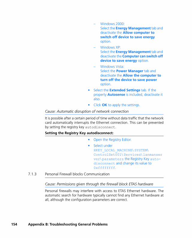
154

– Windows 2000:Select the Energy Management tab and deactivate the Allow computer to switch off device to save energy option.

– Windows XP:Select the Energy Management tab and deactivate the Computer can switch off device to save energy option.

– Windows Vista:Select the Power Manager tab and deactivate the Allow the computer to turn off the device to save power option.

• Select the Extended Settings tab. If the property Autosense is included, deactivate it also.

• Click OK to apply the settings.

Cause: Automatic disruption of network connection

It is possible after a certain period of time without data traffic that the networkcard automatically interrupts the Ethernet connection. This can be preventedby setting the registry key autodisconnect.

Setting the Registry Key autodisconnect:

• Open the Registry Editor.

• Select under HKEY_LOCAL_MACHINE\SYSTEM\ControlSet001\Services\lanmanserver\parameters the Registry Key auto-disconnect and change its value to 0xffffffff.

7.1.3 Personal Firewall blocks Communication

Cause: Permissions given through the firewall block ETAS hardware

Personal firewalls may interfere with access to ETAS Ethernet hardware. Theautomatic search for hardware typically cannot find any Ethernet hardware atall, although the configuration parameters are correct.


Certain actions in ETAS products may lead to some trouble if the firewall is notproperly parameterized, e.g. upon opening an experiment in ASCET or search-ing for hardware from within INCA or HSP.

If a firewall is blocking communication to ETAS hardware, you must either dis-able the firewall software while working with ETAS software, or the firewallmust be configured to give the following permissions:

• Outgoing limited IP broadcasts via UDP (destination address 255.255.255.255) for destination ports 17099 or 18001

• Incoming limited IP broadcasts via UDP (destination IP 255.255.255.255, originating from source IP 0.0.0.0) for destination port 18001

• Directed IP broadcasts via UDP to the network configured for the ETAS application, destination ports 17099 or 18001

• Outgoing IP unicasts via UDP to any IP in network configured for the ETAS application, destination ports 17099 through 18020

• Incoming IP unicasts via UDP originating from any IP in the network configured for the ETAS application, source ports 17099 through 18020, destination ports 17099 through 18020

• Outgoing TCP/IP connections to the network configured for the ETAS application, destination ports 18001 through 18020

Windows XP and Windows Vista come with a built-in personal firewall. Onmany other systems it is very common to have personal firewall software fromthird party vendors, such as Symantec, McAffee or BlackIce installed. The pro-ceedings in configuring the ports might differ for each personal firewall soft-ware used. Therefore please refer to the user documentation of your personalfirewall software for further details.

As an example for a firewall configuration, you will find below a description onhow to configure the widely used Windows XP/Vista firewall if the hardwareaccess is prohibited under Windows XP with Service Pack 2 or Windows Vista.

Note

The ports that have to be used in concrete use cases depend on the hard-ware used. For more precise information on the port numbers that can be used please refer to your hardware documentation.


156

Solution for Windows XP and Vista Firewall, Users with Administrator Priv-ileges

If you have administrator privileges on your PC, the following dialog windowopens if the firewall blocks an ETAS product.

To unblock a product:

• In the "Windows Security Alert" dialog win-dow, click on Unblock.

The firewall no longer blocks the ETAS product in question (in the example: ASCET). This deci-sion survives a restart of the program, or even the PC.

Instead of waiting for the "Windows Security Alert" dialog window, you canunblock ETAS products in advance.

Unblocking ETAS products in the firewall control:

1. Windows XP:

• From the Windows Start Menu, select Settings → Control Panel.

• In the control panel, double-click the Win-dows Firewall icon to open the "Windows Firewall" dialog window.

2. Windows Vista:

• From the Windows Start Menu, select Settings → Control Panel → Security → Windows Firewall.


• In the "Windows Firewall" window, click on Allow program through Windows Fire-wall to open the "Windows Firewall Settings" window.

3. both

• In the "Windows Firewall [Settings]" dialog window, open the "Exceptions" tab.

This tab lists the exceptions not blocked by the firewall. Use Add Program or Edit to add new programs, or edit existing ones.

• Make sure that the ETAS products and services you want to use are properly configured exceptions.


158

– Open the "Change Setup" (XP) or "Change Scope" (VISTA) window.

– To ensure proper ETAS hardware access, make sure that at least the IP addresses 192.168.40.xxx are unblocked.

– Close the "Change Setup" or "Change Scope" window with OK.

• Close the "Windows Firewall" dialog window with OK.

The firewall no longer blocks the ETAS prod-uct in question. This decision survives a restart of the PC.

Solution for Windows XP/Vista Firewall, Users without Administrator Privi-leges

This section addresses users with restricted privileges, e.g., no system changes,write restrictions, local login.

Working with an ETAS software product requires "Write" and "Modify" privi-leges within the ETAS, ETASData, and ETAS temporary directories. Other-wise, an error message opens if the product is started, and a database isopened. In that case, no correct operation of the ETAS product is possiblebecause the database file and some *.ini files are modified during opera-tion.

The ETAS software has to be installed by an administrator anyway. It is recom-mended that the administrator assures that the ETAS program/processes areadded to the list of the Windows XP/Vista firewall exceptions, and selected inthat list, after the installation. If this is omitted, the following will happen:


• The "Window Security Alert" window opens when one of the actions conflicting with a restrictive firewall configuration is executed.

To unblock a program (no Admin privileges):

• In the "Windows Security Alert" dialog win-dow, activate the option For this program, don’t show this message again.

• Click OK to close the window.

An administrator has to select the respective ETAS software in the "Exceptions" tab of the "Windows Firewall" dialog window (Win-dows XP) or the corresponding window in Windows Vista to avoid further problems regarding hardware access with that ETAS product.


160

8 Appendix C: AUTOSAR

8.1 Basic Principles

The creation of an atomic software component in AUTOSAR is done in twosteps. In the first step, the interface of the component is defined. The interfaceis specified in an authoring tool and exchanged via XML. The XML file(s) arethen given to a component API generator which transforms the interfacedescription into a header file. This header file contains all access macros whichthe internal behavior of the atomic software component has to use. As a rule,the component API generator is the contract phase part of an RTE1 generator.

In a second step, the application software component developer provides theinternal behavior in terms of C files respecting and using the interfaces asdefined in the header file. Now the *.h and the *.c file of the atomic soft-ware components are defined and can be compiled for checking. The accessmacros will only be resolved during the RTE generation phase where the RTEgenerator knows the OS schedule and all component (instances) mapped tothe ECU the RTE is generated for.

For atomic software components, ASCET can be used as authoring tool andbehavioral modeling tool. In the authoring approach, the AUTOSAR modelingelements supported in ASCET 6.0, i.e. Modegroup, Interface, Atomic SoftwareComponent, are created and maintained in the ASCET database. This meansthat these elements have an ASCET OID, can carry different implementationsand data and can be (re-)used in several projects.

AUTOSAR elements reference each other in an XML file. For example, dataelement prototypes have a type and are used in sender-receiver interface types.In the same manner, interface types are used as port prototype in atomic soft-ware component types. In ASCET 6.0, one creates atomic software componenttypes. Atomic software components have a so-called internal behavior. Theinternal behavior is composed of runnable entities. Runnable entities resembleASCET processes because in an AUTOSAR ECU integration they are mapped tooperating system tasks, hence, they represent a "partial" behavior of the com-ponent.

ASCET can be used as behavioral modelling tool too. In ASCET 6.0, the internalbehavior of atomic software components is specified by means of a block dia-gram editor. The internal behavior can consist of variables, class instances,parameters and sequence calls. Messages and modules are supported formigration purposes too.

1. runtime environment

Appendix C: AUTOSAR 161

162

AUTOSAR XML and code generation is performed by ASCET projects. Thismeans that the ASCET project in the AUTOSAR use case will contain ONEatomic software component type. AUTOSAR code generation works exclu-sively for the target RTE-AUTOSAR which is a production code target. Duringcode generation, the C code with access macros are found in the cgen-folderof ASCET. If one wants to obtain both the generated *.c and *.arxml files,one has to use the export-generated-code feature of ASCET.

8.2 AUTOSAR Modelling Elements in ASCET

8.2.1 Modes

ASCET supports the AUTOSAR mode management as of release 2.1. A modetype resembles an ASCET enumeration because it has so-called mode declara-tions. Typical mode declarations are init, run, diagnostics, etc. In contrast toenumerations, the representing integer cannot be set explicitly. Modes aremaintained in the database; the first mode declaration in the editor is the initmode.

8.2.2 Interfaces

In ASCET V6.0, only sender-receiver interfaces are supported. Sender-receiverinterfaces resemble, from their editor, layout classes without methods. Sender-receiver interfaces have data element prototypes. The data element prototypesare of an ASCET model type, which means that an interface type can haveseveral ASCET implementations. The ASCET implementation of a sender-receiver interface is defined by the implementation of its data element proto-types. The ASCET implementation of the data element prototype defines anASCET implementation type (e.g. uint16) to an ASCET model type (e.g.cont). The range of the ASCET implementation type is given by the physicalrange of the model type cont and the applied implementation formula. Therange of the ASCET implementation type determines the primitive AUTOSARtype of the data element prototype. In AUTOSAR release 2.1, the RTE thentranslates the AUTOSAR types in C types. This translation is described in sec-tion 5.2.4.2 in the RTE specification1. These data types match with implemen-tation types of ASCET.

All available built-in ASCET model types as well as the user-defined types enu-meration and record can be chosen as data type for a data element prototype.Arrays cannot be directly used, they have to be encapsulated in a record.Modes can only be used in sender-receiver interfaces when there are no otherdata element prototypes with another type but mode. This means that if asender-receiver interfaces contains modes as data element prototypes, then all

1. AUTOSAR_SWS_RTE release 2.1, available at www.autosar.org.

Appendix C: AUTOSAR

http://www.autosar.org

data element prototypes must be of type mode. And for these mode inter-faces, the data element prototypes are called mode declaration group proto-type.

8.2.3 Atomic Software Component Types

Atomic software components are a mixture of hierarchical ASCET classes andmodules. An atomic software component (SWC) can instantiate interfacetypes as so-called port prototype. This means that within one SWC there mightbe several port prototypes with the same interface type. port prototypes canbe provided or required, thus realizing a role. A port prototype with a sender-receiver interface is a required port if the data element prototypes are"received" by the component. A port prototype with a sender-receiver inter-face is a provided port if the data-elements are "sent" by the component.

Port prototypes are elements of a SWC and hence their role can be selected inthe properties editor. If the role is set appropriately, the data element proto-types resemble to ASCET messages. While sending and receiving of messagesin ASCET modules is performed by messages, AUTOSAR SWCs use runnable-entities to perform the access to the data element prototypes of port proto-types.

The internal behavior of SWCs is therefore given by a number of runnableentities. Each time a runnable entity reads a data element prototype, it per-forms a data-read access. A similar scheme can be found for the sending ofdata element prototypes where a data-write access is performed by the runna-ble entity. In contrast to ASCET messages, there are different flavors of data-element access. The most common flavors are implicit and explicit.

In the elements list of a SWC in ASCET, the port prototypes appear as well asall other included elements like variables, parameters, class instances, modulesand messages. SWCs have diagrams, too. Runnable entities are defined in dia-grams. Besides runnable entites, an ASCET SWC also supports methods.

Runnable entities use sequence calls to model graphical assignments. Forexample, to read a data element prototype implicitly, the port prototype isdrawn to a diagram. Now, one can connect the pin of the data element proto-type to operations of an expression, which might end up in a variable or in awrite access to data element prototype in a provided port. The assignment willbe performed by a sequence call, and the sequence call is triggered by a run-nable entity (or by a method). Explicit data-read access, also called data-receivepoint, will need a dedicated access operator and a variable or message wherethe data is stored. The sequence call of the variable or the message will have arunnable entity or a method as trigger.


164

8.3 Applying ASCET Implementations to AUTOSAR

As written above, data element prototypes of sender-receiver interfaces inASCET are supporting ASCET model types whereas the AUTOSAR type canonly be determined after the ASCET model type has been implemented. Inparticular, this means that one sender-receiver interface entry in the ASCETdatabase will represent as many different AUTOSAR interface types as thereare implementations of the ASCET interface! Since SWCs in ASCET employASCET sender-receiver interfaces in their port prototypes, they have differentimplementations, too. As a result, one ASCET atomic software componenttype will has as many different AUTOSAR atomic software component type asthere are ASCET implementations defined.

8.3.1 Subpackages

AUTOSAR in its release 2.1 only supports shortnames of 32 character length inits XML description. This means that the classical ASCET approach to distin-guish different implementations in the generated code by concatenating theimplementation name to the ASCET model name has its limitations. This limi-tation is overcome by the introduction of subpackages in the XML file. There isone package generated for the atomic software component as well as theinterface, but before going to the elements there will be a subpackage foreach implementation. ASCET 6.0 will only generate C code and the XMLdescription for one implementation of the atomic software component; hencethere will be only one subpackage. The implementation is selected at theproject prior to code generation. The ASCET XML generator takes care that allreferences are set appropriately, e.g. the type reference from a port prototypein subpackage impl-1 to an interface in subpackage impl-2. Please notethat atomic SWC and the interfaces are different AUTOSAR packages.

8.4 Example

In a very simple example, a very simple atomic software component has twoport prototoypes for data communication (port2 with interface type IF_aand port4 with interface type IF_AB). On top of these ports, there is a modeport. The software component has two runnable enties, runnable_expland runnable_impl. The elements of the atomic software components are

Appendix C: AUTOSAR

shown in Fig. 8-1. Besides the AUTOSAR elements, there is an error variableto be examined by the runnable entity with explicit data-access, and an enu-meration return type tailored for RTE-access.

Fig. 8-1 Elements of a simple atomic software component

Interface IF_a and interface IF_ab group data element prototypes of theembedded ASCET model type cont. This is shown for interface type a inFig. 8-2, where one sees, in the left, the data element prototypes in the ele-ments list.

If one selects the AR_16bit implementation, and then has a look at the"Implementation" tab, one sees that with a chosen conversion formula theimplementation type has changed to a signed 16 bit integer. For this setting,the code as well as the AUTOSAR XML files are generated.

An excerpt of the generated XML file is shown in Fig. 8-4: First of all, onerecognizes the subpackage AR_16bit below the AR-Package ASCETinterfaces. The data element prototype a is embedded in the AR_16bitsubpackage and (type-)references the implementation type sint16 from theautosar_types.arxml file.

Fig. 8-2 Interface IF_a

Fig. 8-3 Interface IF_a with integer implementation


166

Fig. 8-4 Generated Interface in AR_16bit Subpackage

As written above and shown in Fig. 8-1, the port prototype of the nameport2 is of the interface type IF_a. As with all ASCET modelling elements,atomic software component have several implementations when used for pro-duction code generation. In this example, the AR_VerySimpleExamplecomponent has two implementations. First, there is the real 64 bit defaultimplementation impl for the continuous model, whereas the AR_16bitimplementation uses signed int16 types. In this example, the integer imple-mentation was chosen for code generation as shown in Fig. 8-5.

Fig. 8-5 Selection of the 16 bit integer implementation

Appendix C: AUTOSAR

An excerpt of the generated AUTOSAR XML file is shown in Fig. 8-6. Theatomic software component AR_VerySimpleExample is embedded in thesubpackage which has the same name as the ASCET implementation.

Fig. 8-6 Generated Atomic Software Component in AR_16bit Subpack-age

From the AUTOSAR package point of view, using this kind of ASCET imple-mentation representation requires that the type references for all aggregatedelements will find its appropriate package. An example for this kind of "sub-package-referencing" is shown in Fig. 8-7. To find the interface IF_a in itsAR_16bit implementation, the type-reference of port2 in the atomic soft-ware component AR_VerySimpleExample references not only to theASCET_interfaces package, but also to its subpackage AR_16bit.

An authoring or ECU integration tool is expected to work with subpackages.Please keep in mind that the subpackage structure does not have any influenceon the code generation or the RTE access itself.


168

The reason for choosing the sub-package representation lies in the 32-charac-ter limitation of AUTOSAR Release 2.1. The classical ASCET way of concatenat-ing element name and implementation name is seen as too restrictive.

Fig. 8-7 Subpackage Referencing in AUTOSAR XML Files

The internal behavior of ASCET software components is realized by means ofthe block diagram editor. In this example, there are two diagrams holding onerunnable entity each. In the first diagram, there is a runnable entity realizingonly implicit access to the port prototypes port2 and port4. The correspond-ing block diagram is shown in Fig. 8-8. The require port prototype port2 isshown on the left side. Its data element prototype a is accessed by thesequence call number 5 of the runnable entity runnable_impl and used inthe graphical expression. The result of this expression is written to the dataelement prototype a of the port prototype port4 by the sequence call num-ber 5. Data element prototype a of port prototype port2 is also accessed bythe sequence call number 10 whose expression just adds 1 (in the physicalmodel) to a and writes the result implicitly to the data element prototype b ofthe port prototype port4.

Fig. 8-8 Internal Behavior of the "Implicit" Runnable-Entity

Appendix C: AUTOSAR

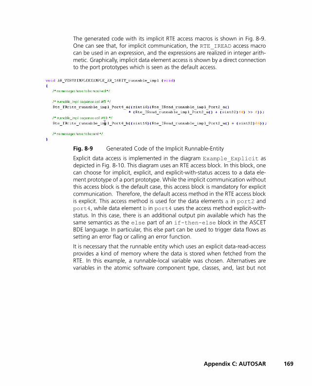
The generated code with its implicit RTE access macros is shown in Fig. 8-9.One can see that, for implicit communication, the RTE_IREAD access macrocan be used in an expression, and the expressions are realized in integer arith-metic. Graphically, implicit data element access is shown by a direct connectionto the port prototypes which is seen as the default access.

Fig. 8-9 Generated Code of the Implicit Runnable-Entity

Explicit data access is implemented in the diagram Example_Explicit asdepicted in Fig. 8-10. This diagram uses an RTE access block. In this block, onecan choose for implicit, explicit, and explicit-with-status access to a data ele-ment prototype of a port prototype. While the implicit communication withoutthis access block is the default case, this access block is mandatory for explicitcommunication. Therefore, the default access method in the RTE access blockis explicit. This access method is used for the data elements a in port2 andport4, while data element b in port4 uses the access method explicit-with-status. In this case, there is an additional output pin available which has thesame semantics as the else part of an if-then-else block in the ASCETBDE language. In particular, this else part can be used to trigger data flows assetting an error flag or calling an error function.

It is necessary that the runnable entity which uses an explicit data-read-accessprovides a kind of memory where the data is stored when fetched from theRTE. In this example, a runnable-local variable was chosen. Alternatives arevariables in the atomic software component type, classes, and, last but not


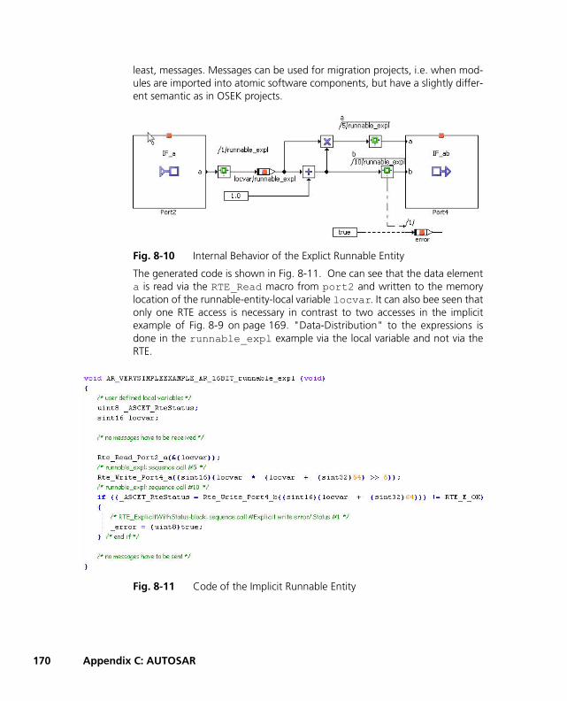
170

least, messages. Messages can be used for migration projects, i.e. when mod-ules are imported into atomic software components, but have a slightly differ-ent semantic as in OSEK projects.

Fig. 8-10 Internal Behavior of the Explict Runnable Entity

The generated code is shown in Fig. 8-11. One can see that the data elementa is read via the RTE_Read macro from port2 and written to the memorylocation of the runnable-entity-local variable locvar. It can also bee seen thatonly one RTE access is necessary in contrast to two accesses in the implicitexample of Fig. 8-9 on page 169. "Data-Distribution" to the expressions isdone in the runnable_expl example via the local variable and not via theRTE.

Fig. 8-11 Code of the Implicit Runnable Entity

Appendix C: AUTOSAR

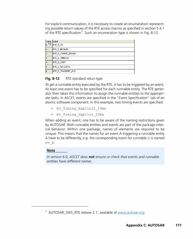
For explicit communication, it is necessary to create an enumeration represent-ing possible return values of the RTE access macros as specified in section 5.4.1of the RTE specification1. Such an enumeration type is shown in Fig. 8-12.

Fig. 8-12 RTE standard retun-type

To get a runnable entity executed by the RTE, it has to be triggered by an event.At least one event has to be specified for each runnable entity. The RTE gener-ator then takes this information to assign the runnable entities to the appropri-ate tasks. In ASCET, events are specified in the "Event Specification" tab of anatomic software component. In this example, two timing events are specified:

• Ev_Timing_Explicit_10ms

• Ev_Timing_Implict_10ms

When adding an event, one has to be aware of the naming restrictions givenby AUTOSAR. Both runnable entities and events are part of the package-inter-nal behavior. Within one package, names of elements are required to beunique. This means that the names for an event A triggering a runnable entityA have to be differently, e.g. the corresponding event for runnable A is namedev_A.

1. AUTOSAR_SWS_RTE release 2.1, available at www.autosar.org.

Note

In version 6.0, ASCET does not ensure or check that events and runnable entities have different names.


http://www.autosar.org

172

The association between the explicit timing event and the explicit runnableentity is shown in Fig. 8-13.

Fig. 8-13 Mapping of Events to Runnable Entities

The AUTOSAR runtime execution concept has the notations of modes. Forapplication software components, the execution of a runnable entity can becoupled to a so-called mode-disabling dependency. It defines under whichmodes the RTE will NOT execute a runnable entity. Modes are communicatedto an atomic software component by means of port prototypes.

In this example, there are two modes defined. This is achieved by creating amode declaration group (or mode group for short) with the name OnOff-Mode, see Fig. 8-14.

Fig. 8-14 Mode Declaration Group

This mode group is instantiated in a sender-receiver interface namedModeInterface as mode declaration group prototype, as shown inFig. 8-15. The ModeInterface is then instantiated in a port prototoypecalled ModePort in the atomic software component of this example. It can beseen in the elements list in Fig. 8-1 on page 165.

Fig. 8-15 Mode Declaration Group Prototype in a Sender-Receiver Interface

Appendix C: AUTOSAR

The association of modes with RTE events is done automatically, meaning thatwhen an atomic software component type has aggregated a port prototypewith a "mode interface", then all runnable entitites of this component areassumed to be associated to a mode-disabling dependency. The constellationshown in Fig. 8-16 means that the event ev_timingExpl_10ms is enabledin OnMode while the event ev_timingImpl_10ms is enabled in OffMode.

Fig. 8-16 Event Specification Editor

8.5 Migration of Legacy Projects

The classical modelling means of ASCET are modules and classes. Both meanscan still be used in atomic software components. Fig. 8-17 shows a possibilityhow to re-use a module. The module is named SimpleMigrationModule.Its message receive_a has its set method activated and the messagessend_a and send_b have their get method enabled. In this case, the mes-sages become "visible" in the atomic software component as send/receivemessages. As a result, the receive message in the module can be used to storethe data element prototype a of port2 from the data-receive point of therunnable entity migration_runnable_module_10ms. The send mes-sages of the module can be used as arguments in the data-send points.


174

Fig. 8-17 Integration of a Module into an Atomic Software Component

As one can see from sequence call number 5, processes can be called likemethods in the block diagram editor of the atomic software component. Thegenerated code is shown in Fig. 8-18. From the module point of view, allreceive messages are read from the RTE, then the processes are called whilethe send messages are written to the RTE.

Fig. 8-18 Generated Code of a Module in an Atomic Software Component

As can be seen in Fig. 8-19, the algorithm in the process is not aware of beingused in an atomic software component type. This means that existing modulesand even projects can be migrated easily to one atomic software componenttype. In case of two runnable entities calling two processes sharing a commonmessage, the ASCET code generator will guard the message by generating asurrounding exclusive area. The concept of inter-runnable variable is not sup-

Appendix C: AUTOSAR

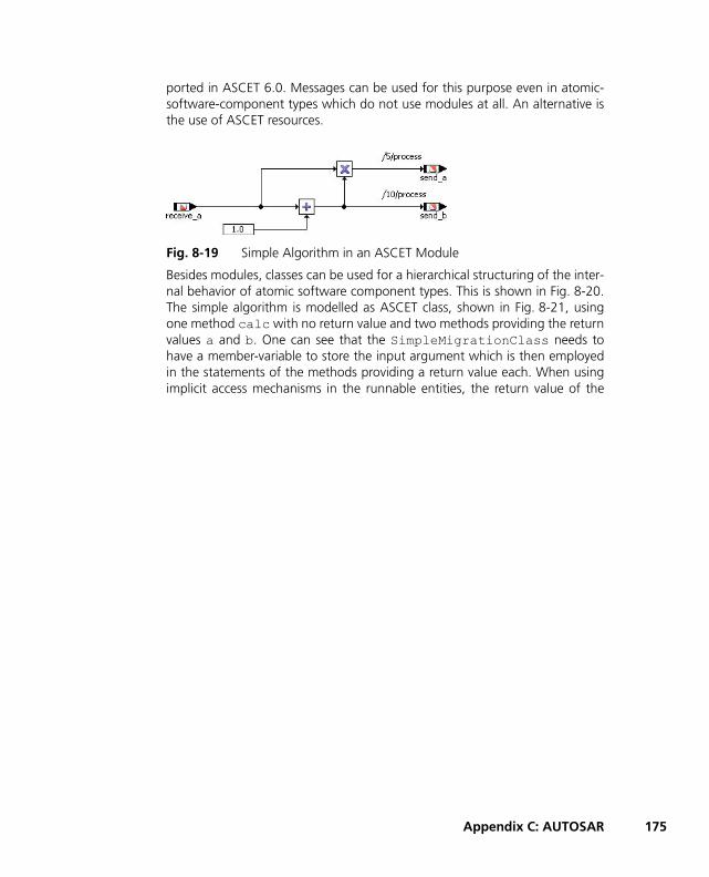
ported in ASCET 6.0. Messages can be used for this purpose even in atomic-software-component types which do not use modules at all. An alternative isthe use of ASCET resources.

Fig. 8-19 Simple Algorithm in an ASCET Module

Besides modules, classes can be used for a hierarchical structuring of the inter-nal behavior of atomic software component types. This is shown in Fig. 8-20.The simple algorithm is modelled as ASCET class, shown in Fig. 8-21, usingone method calc with no return value and two methods providing the returnvalues a and b. One can see that the SimpleMigrationClass needs tohave a member-variable to store the input argument which is then employedin the statements of the methods providing a return value each. When usingimplicit access mechanisms in the runnable entities, the return value of the


176

data read access macro can directly be used as argument in the calc method,and the return values of the other methods can directly be used in the datawrite access macros. The generated code is shown in Fig. 8-22.

Fig. 8-20 Use of an ASCET Class Instance with several methods in an Atomic Software Component

Fig. 8-21 Simple Algorithm partitioned into methods

Fig. 8-22 Generated Code when using a class with classic ASCET methods

Besides the classical method modelling of classes, ASCET 6.0 provides out-parameters in methods. This feature is used in Fig. 8-23, where a methodcalc_return with one input and two output arguments is used instead ofthree classical ASCET methods in Fig. 8-20.

Appendix C: AUTOSAR

As in C or other programming languages, the output parameters are passed byreference to the methods. This means that memory has to be allocated beforecalling the method. In this example, there are two local variables (return_aand return_b) of the migration_runnable_Expl_class_10mswhere the results of the algorithm are written to. The algorithm itself is shownin Fig. 8-24. Since it works exclusively on argument values, it does not need anadditional member-variable as the algorithm shown in Fig. 8-21 on page 176.

Since additional variables, even as runnable-local variables, are necessary at all,explicit communication appears to be the preferred solution for RTE access.Therefore, an additional (runnable-local) variable arg_a is used in this exam-ple. The generated code is shown in

Fig. 8-23 Use of an ASCET class Instance with one method

Fig. 8-24 Simple Algorithm in one Method


178

Fig. 8-25 Generated Code for an Atomic-Software Component using an ASCET class instance with one method

Appendix C: AUTOSAR

9 ETAS Contact Addresses

ETAS HQ

ETAS GmbH

ETAS Subsidiaries and Technical Support

For details of your local sales office as well as your local technical support teamand product hotlines, take a look at the ETAS website:

Borsigstraße 14 Phone: +49 711 89661-0

70469 Stuttgart Fax: +49 711 89661-106

Germany WWW: www.etas.com

ETAS subsidiaries WWW: www.etas.com/en/contact.php

ETAS technical support WWW: www.etas.com/en/hotlines.php

ETAS Contact Addresses 179

http://www.etasgroup.com



http://www.etas.com

http://www.etas.com/en/contact.php

http://www.etas.com/en/hotlines.php

180
ETAS Contact Addresses

Index
Aapplication mode 139ASAM-MCD-2MC file 139ASCET
AUTOSAR elements 36atomic software component type 163AUTOSAR 33–39, 161–178

atomic software component type 163

elements in ASCET 36interface 37interfaces 162modes 162Overview 33port 37port prototype 163Pport 37Rport 38runnable entity 38runtime environment 34, 35, 39sender-receiver communication 38software component 33, 37virtual function bus 33

AUTOSAR interface 37

CC code 140calibration windows 140characteristic line 140characteristic map 140characteristic value 140class 140component 141Component Manager 141condition 141Configuration dialog box 141

Ddata 141data generator 141data logger 141data set 142database 142description file 142diagram 142dimension 142Distribution 142

181

182

Eeditor 142

element 181element 142element editor

open 181environment 143error

continue 150exit 150support function "Problem

Report" 149System Error window 149what to do in case of ~ 150

ETAS Contact Addresses 179event 142event generator 142experiment 143experiment environment 143

Ffixed point code 143folder 143formula 143fullpass experiment 143

GGeneral Operation

monitor window 11supporting functions 11

Glossary 137–148

HHEX file 143hierarchy 143

Iicon 144implementation 144Intel Hex 144interface 37, 144

Kkind 144

Llayout 145literal 145

Mmeasure 145measure window 145measured signal 145measurement 145measuring channel parameters 145message 145methods 145model type 145module 146monitor 146Motorola-S-Record 146

OOscilloscope 146

Pparameter 146port

AUTOSAR 37port prototype 163Pport 37priority 147Problem Report 149process 147program 147program description 147project 147

Rresource 147Rport 38runnable entity 38runtime environment 34, 35, 39

Sscheduling 147scope 147sender-receiver communication 38software component 37state 147State machine 148

Index

support function "Problem Report" 149

Ttarget 148task 148Transition 148type 148

Uuser profile 148

Vvariables 148virtual function bus 33

Wwindow elements 148

Index 183

184
Index

ascet v6.0 getting started - etas · pdf file4.6.1 motion equation ... reductions a reality....

Documents