asme ptc 18-2011-hydraulic turbines and pump-turbines-performance test codes

Hydraulic Turbines and Pump-TurbinesPerformance Test Codes

A N I N T E R N A T I O N A L C O D E

ASME PTC 18-2011(Revision of ASME PTC 18-2002)

Copyright ASME International Provided by IHS under license with ASME No reproduction or networking permitted without license from IHS

--`,`,,`,`,``,,`,````,,`,````-`-`,,`,,`,`,,`---

INTENTIONALLY LEFT BLANK


--`,`,,`,`,``,,`,````,,`,````-`-`,,`,,`,`,,`---

ASME PTC 18-2011

Hydraulic Turbines and Pump-Turbines

Performance Test Codes

A N I N T E R N A T I O N A L C O D E

(Revision of ASME PTC 18-2002)

Three Park Avenue • New York, NY • 10016 USA


--`,`,,`,`,``,,`,````,,`,````-`-`,,`,,`,`,,`---

Date of Issuance: June 10, 2011

The next edition of this Code is scheduled for publication in 2016. There will be no addenda issued to this edition.

ASME issues written replies to inquiries concerning interpretations of technical aspects of this Code. Interpretations are published on the ASME Web site under the Committee Pages at http://cstools.asme.org as they are issued.

ASME is the registered trademark of The American Society of Mechanical Engineers.

This code or standard was developed under procedures accredited as meeting the criteria for American National Standards. The Standards Committee that approved the code or standard was balanced to assure that individuals from competent and concerned interests have had an opportunity to participate. The proposed code or standard was made available for public review and comment that provides an opportunity for additional public input from industry, academia, regulatory agencies, and the public-at-large.

ASME does not approve, rate, orendorse any item, construction, proprietary device, or activity.ASME does not take any position with respect to the validity of any patent rights asserted in connection with any items mentioned in this

document, and does not undertake to insure anyone utilizing a standard against liability for infringement of any applicable letters patent, nor assumes any such liability. Users of a code or standard are expressly advised that determination of the validity of any such patent rights, and the risk of infringement of such rights, is entirely their own responsibility.

Participation by federal agency representative(s) or person(s) affiliated with industry is not to be interpreted as government or industry endorsement of this code or standard.

ASME accepts responsibility for only those interpretations of this document issued in accordance with the established ASME procedures and policies, which precludes the issuance of interpretations by individuals.

No part of this document may be reproduced in any form,in an electronic retrieval system or otherwise,

without the prior written permission of the publisher.

The American Society of Mechanical EngineersThree Park Avenue, New York, NY 10016-5990

Copyright © 2011 byTHE AMERICAN SOCIETY OF MECHANICAL ENGINEERS

All rights reservedPrinted in U.S.A.


--`,`,,`,`,``,,`,````,,`,````-`-`,,`,,`,`,,`---

iii

CONTENTS

Notice .................................................................................................................................................................................... vForeword .............................................................................................................................................................................. viCommittee Roster ................................................................................................................................................................ viiiCorrespondence With the PTC 18 Committee ................................................................................................................ ix

Section 1 Object and Scope .................................................................................................................................... 11-1 Object ............................................................................................................................................................... 11-2 Scope ................................................................................................................................................................ 11-3 Uncertainties .................................................................................................................................................. 1

Section 2 Definitions and Descriptions of Terms .................................................................................................... 22-1 Definitions ...................................................................................................................................................... 22-2 International System of Units (SI) ............................................................................................................... 22-3 Tables and Figures ......................................................................................................................................... 22-4 Reference Elevation, Zc ................................................................................................................................. 22-5 Centrifugal Pumps ........................................................................................................................................ 22-6 Subscripts Used Throughout the Code ...................................................................................................... 3

Section 3 Guiding Principles ................................................................................................................................... 263-1 General ............................................................................................................................................................ 263-2 Preparations for Testing ................................................................................................................................ 263-3 Tests ................................................................................................................................................................. 283-4 Instruments ..................................................................................................................................................... 293-5 Operating Conditions ................................................................................................................................... 293-6 Data Records .................................................................................................................................................. 29

Section 4 Instruments and Methods of Measurement ............................................................................................ 324-1 General ............................................................................................................................................................ 324-2 Electronic Data Acquisition .......................................................................................................................... 324-3 Head and Pressure Measurement ............................................................................................................... 334-4 Flow Measurement ........................................................................................................................................ 374-5 Power Measurement ..................................................................................................................................... 584-6 Speed Measurement ...................................................................................................................................... 624-7 Time Measurement ........................................................................................................................................ 63

Section 5 Computation of Results ........................................................................................................................... 645-1 Measured Values: Data Reduction ............................................................................................................. 645-2 Conversion of Test Results to Specified Conditions ................................................................................. 645-3 Evaluation of Uncertainty ............................................................................................................................ 655-4 Comparison With Guarantees ..................................................................................................................... 65

Section 6 Final Report ............................................................................................................................................. 676-1 Responsibility of Chief of Test ..................................................................................................................... 676-2 Parties to the Test ........................................................................................................................................... 676-3 Acceptance Tests ............................................................................................................................................ 67

Figures2-3-1 Head Definition, Measurement and Calibration, Vertical Shaft Machine With

Spiral Case and Pressure Conduit ............................................................................................................ 202-3-2 Head Definition, Measurement and Calibration, Vertical Shaft Machine

With Semi-Spiral Case ................................................................................................................................ 212-3-3 Head Definition, Measurement and Calibration, Bulb Machine .............................................................. 222-3-4 Head Definition, Measurement and Calibration, Horizontal Shaft Impulse

Turbine (One or Two Jets) ......................................................................................................................... 23


--`,`,,`,`,``,,`,````,,`,````-`-`,,`,,`,`,,`---

iv

2-3-5 Head Definition, Measurement and Calibration, Vertical Shaft Impulse Turbine ................................. 242-4-1 Reference Elevation, Zc, of Turbines and Pump-Turbines ......................................................................... 253-5.3-1 Limits of Permissible Deviations From Specified Operating Conditions in Turbine Mode ................. 303-5.3-2 Limits of Permissible Deviations From Specified Operating Conditions in Pump Mode .................... 314-3.14-1 Pressure Tap...................................................................................................................................................... 354-3.15-1 Calibration Connections for Pressure Gages or Pressure Transducers .................................................... 364-4.3.4-1 Example of Digital Pressure–Time Signal .................................................................................................... 414-4.4.1-1 Ultrasonic Method: Diagram to Illustrate Principle ................................................................................... 434-4.4.1-2 Ultrasonic Method: Typical Arrangement of Transducers for an 8-Path

Flowmeter in a Circular Conduit .............................................................................................................. 444-4.4.3-1 Ultrasonic Method: Typical Arrangement of Transducers ........................................................................ 464-4.4.4-1 Distortion of the Velocity Profile Caused by Protruding Transducers .................................................... 474-4.4.6-1 Ultrasonic Method: Typical Arrangement of Transducers for an

18-Path Flowmeter in a Circular Conduit ................................................................................................ 494-4.4.6-2 Ultrasonic Method: Typical Arrangement of Transducers for an 18-Path

Flowmeter in a Rectangular Conduit ....................................................................................................... 504-4.4.11-1 Locations for Measurements of D ................................................................................................................. 524-4.5.1-1 Schematic Representation of Dye Dilution Technique ............................................................................... 544-4.5.2.1-1 Experimental Results: Allowable Variation in Tracer Concentration ...................................................... 554-4.5.5-1 Typical Chart Recording During Sampling ................................................................................................. 574-5.1-1 Three-Wattmeter Connection Diagram ........................................................................................................ 594-5.1-2 Two-Wattmeter Connection Diagram ........................................................................................................... 604-5.1-3 Measuring Instrument Burden ...................................................................................................................... 61

Tables2-2-1 Conversion Factors Between SI Units and U.S. Customary Units of Measure....................................... 32-3-1 Letter Symbols and Definitions ..................................................................................................................... 42-3-2M Acceleration of Gravity as a Function of Latitude and Elevation, SI Units (m/s2)................................ 102-3-2 Acceleration of Gravity as a Function of Latitude and Elevation,

U.S. Customary Units (ft/sec2) .................................................................................................................. 112-3-3M Vapor Pressure of Distilled Water as a Function of Temperature, SI Units (kPa) .................................. 112-3-3 Vapor Pressure of Distilled Water as a Function of Temperature,

U.S. Customary Units (lbf/in.2) ................................................................................................................. 122-3-4M Density of Water as a Function of Temperature and Pressure, SI Units (kg/m3)................................... 132-3-4 Density of Water as a Function of Temperature and Pressure,

U.S. Customary Units (slug/ft3) ................................................................................................................ 142-3-5 Coefficients Ii, Ji, and ni ................................................................................................................................... 152-3-6M Density of Dry Air, SI Units (kg/m3) ............................................................................................................ 162-3-6 Density of Dry Air, U.S. Customary Units (slug/ft3) ................................................................................. 162-3-7M Density of Mercury, SI Units (kg/m3) ........................................................................................................... 172-3-7 Density of Mercury, U.S. Customary Units (slugs/ft3) .............................................................................. 182-3-8M Atmospheric Pressure, SI Units (kPa) .......................................................................................................... 192-3-8 Atmospheric Pressure, U.S. Customary Units (lbf/in.2) ............................................................................ 194-4.4.2-1 Integration Parameters for Ultrasonic Method:

Four Paths in One Plane or Eight Paths in Two Planes ......................................................................... 454-4.4.6-1 Integration Parameters for Ultrasonic Method: 18 Paths in Two Planes ................................................. 51

Nonmandatory AppendicesA Typical Values of Uncertainty ........................................................................................................................ 69B Uncertainty Analysis ....................................................................................................................................... 70C Outliers ............................................................................................................................................................. 74D Relative Flow Measurement–Index Test ...................................................................................................... 75E Derivation of the Pressure–Time Flow Integral .......................................................................................... 81


--`,`,,`,`,``,,`,````,,`,````-`-`,,`,,`,`,,`---

v

NOTICE

All Performance Test Codes MUST adhere to the requirements of PTC 1, GENERAL INSTRUCTIONS. The fol-lowing information is based on that document and is included here for emphasis and for the convenience of the user of this Code. It is expected that the Code user is fully cognizant of Parts I and III of PTC 1 and has read them prior to applying this Code.

ASME Performance Test Codes provide test procedures which yield results of the highest level of accuracy con-sistent with the best engineering knowledge and practice currently available. They were developed by balanced committees representing all concerned interests. They specify procedures, instrumentation, equipment operating requirements, calculation methods, and uncertainty analysis.

When tests are run in accordance with a Code, the test results themselves, without adjustment for uncertainty, yield the best available indication of the actual performance of the tested equipment. ASME Performance Test Codes do not specify means to compare those results to contractual guarantees. Therefore, it is recommended that the parties to a commercial test agree before starting the test and preferably before signing the contract on the method to be used for comparing the test results to the contractual guarantees. It is beyond the scope of any Code to determine or interpret how such comparisons shall be made.


--`,`,,`,`,``,,`,````,,`,````-`-`,,`,,`,`,,`---

vi

FOREWORD

The “Rules for Conducting Tests of Waterwheels” was one of a group of ten test codes published by the ASME in 1915. The Pelton Water Wheel Company published a testing code for hydraulic turbines, which was approved by the Machinery Builders’ Society on October 11, 1917. This code included the brine velocity method of measuring flow wherein the time of passage of an injection of brine was detected by electrical resistance. Also in October 1917, the Council of the ASME authorized the appointment of a joint committee to undertake the task of revising the “Rules for Conducting Tests of Waterwheels.” The joint committee consisted of thirteen members, four from the ASME and three each from ASCE, AIEE, and NELA (National Electric Light Association). The code was printed in the April 1922 issue of Mechanical Engineering in preliminary form. It was approved in the final revised form at the June 1923 meeting of the Main Committee and was later approved and adopted by the ASME Council as a standard practice of the Society.

Within three years the 1923 revised edition was out of print and a second revision was ordered by the Main Committee. In November 1925, the ASME Council appointed a new committee, the Power Test Codes Individual Committee No. 18 on Hydraulic Power Plants. This committee organized itself quickly and completed a redraft of the code in time for a discussion with the advisory on Prime Movers of the IEC at the New York meeting later in April 1926. The code was redrafted in line with this discussion and was approved by the Main Committee in March 1927. It was approved and adopted by the ASME Council as the standard practice of the Society on April 14, 1927.

In October 1931 the ASME Council approved personnel for a newly organized committee, Power Test Codes Individual Committee No. 18 on Hydraulic Prime Movers, to undertake revision of the 1927 test code. The commit-tee completed the drafting of the revised code in 1937. The Main Committee approved the revised code on April 4, 1938. The code was then approved and adopted by the Council as standard practice of the Society on June 6, 1938. The term “Hydraulic Prime Movers” is defined as reaction and impulse turbines, both of which are included in the term “hydraulic turbines.” A revision of this Code was approved by the Power Test Codes Committee and by the Council of ASME in August 1942. Additional revisions were authorized by Performance Test Code Committee No. 18 (PTC 18) in December 1947. Another revision was adopted in December 1948. It was also voted to recommend the reissue of the 1938 Code to incorporate all of the approved revisions as a 1949 edition. A complete rewriting of the Code was not considered necessary, because the 1938 edition had been successful and was in general use. A supple-ment was prepared to cover index testing. The revised Code including index testing was approved on April 8, 1949, by the Power Test Codes Committee and was approved and adopted by the Council of ASME by action of the Board on Codes and Standards on May 6, 1949.

The members of the 1938 to 1949 committees included C. M. Allen, who further developed the Salt Velocity Method of flow rate measurement; N. R. Gibson, who devised the Pressure-Time Method of flow rate measurement; L. F. Moody, who developed a method for estimating prototype efficiency from model tests; S. Logan Kerr, successful consultant on pressure rise and surge; T. H. Hogg, who developed a graphical solution for pressure rise; G. R. Rich, who wrote a book on pressure rise; as well as other well known hydro engineers.

In 1963, Hydraulic Prime Movers Test Code Committee, PTC 18, was charged with the preparation of a Test Code for the Pumping Mode/Pump Turbines. The Code for the pumping mode was approved by the Performance Test Codes Supervisory Committee on January 23, 1978, and was then approved as an American National Standard by the ANSI Board of Standards Review on July 17, 1978.

The PTC 18 Committee then proceeded to review and revise the 1949 Hydraulic Prime Movers Code as a Test Code for Hydraulic Turbines. The result of that effort was the publication of PTC 18-1992 Hydraulic Turbines.

Since two separate but similar Codes now existed, the PTC 18 Committee proceeded to consolidate them into a single Code encompassing both the turbine and pump modes of Pump/Turbines. The consolidation also provided the opportunity to improve upon the clarity of the preceeding Codes, as well as to introduce newer technologies such as automated data-acquisition and computation techniques, and the dye-dilution method. Concurrently, the flow methods of salt velocity, pitot tubes and weirs, which had become rarely used, were removed from the 2002 Edition. However, detailed descriptions of these methods remain in previous versions of PTC 18 and PTC 18.1

Following the publication of the 2002 Revision of PTC 18, the PTC 18 Committee began work on the next Revision to further modernize and increase the accuracy of measuring techniques and to improve clarity. The 2011 Revision is characterized by the following features: increased harmonization of text with other ASME Performance Test Codes according to PTC 1 General Instructions; improvement of text and illustrations; modernization of techniques with increased guidance on electronic data acquisition systems and — in the case of the Ultrasonic Method — increasing ultrasonic flow-measurement accuracy with additional paths; deletion from this Code of the seldom used Venturi, volumetric and pressure-time Gibson flow-measurement methods; deletion from this Code of the seldom practical


--`,`,,`,`,``,,`,````,,`,````-`-`,,`,,`,`,,`---

vii

direct method of power measurement; and removal of the Relative Flow Measurement–Index Test from the main text of the Code to a nonmandatory Appendix.

The methods of measuring flow rate included in this Code meet the criteria of the PTC 18 Committee for soundness of principle, have acceptable limits of accuracy, and have demonstrated application under laboratory and field condi-tions. There are other methods of measuring flow rate under consideration for inclusion in the Code at a later date.

This Code was approved by the Board on Standardization and Testing on March 3, 2011, and approved as an American National Standard by the ANSI Board of Standards Review on April 25, 2011.


--`,`,,`,`,``,,`,````,,`,````-`-`,,`,,`,`,,`---

viii

ASME PTC COMMITTEEPerformance Test Codes

(The following is the roster of the Committee at the time of approval of this Code.)

STANDARDS COMMITTEE OFFICERS

J. R. Friedman, ChairJ. W. Milton, Vice ChairJ. H. Karian, Secretary

STANDARDS COMMITTEE PERSONNEL

P. G. Albert, General Electric Co. R. R. Priestley, ConsultantR. P. Allen, Consultant J. A. Silvaggio, Siemens Demag Delaval, Inc.J. M. Burns, Burns Engineering, Inc. W. G. Steele, Mississippi State UniversityW. C. Campbell, Southern Company Services, Inc. T. L. Toburen, T2E3, Inc.M. J. Dooley, Alstom Power, Inc. G. E. Weber, Midwest Generation EME LLCJ. R. Friedman, Siemens Energy, Inc. J. C. Westcott, Mustan Corp.G. J. Gerber, Consultant W. C. Wood, Duke Energy, Inc.P. M. Gerhart, University of Evansville T. K. Kirpatrick, Alternate, McHale & Associates, Inc.T. C. Heil, Consultant S. A. Scavuzzo, Alternate, Babcock & Wilcox Com.R. A. Henry, Sargent & Lundy, Inc. R. L. Bannister, Honorary Member, ConsultantJ. H. Karian, The American Society of Mechanical Engineers W. O. Hays, Honorary Member, ConsultantD. R. Keyser, Survice Engineering R. Jorgensen, Honorary Member, ConsultantS. J. Korellis, Electric Power Research Institute F. H. Light, Honorary Member, ConsultantM. P. McHale, McHale & Associates, Inc. G. H. Mittendorf, Jr., Honorary Member, ConsultantP. M. McHale, McHale & Associates, Inc. J. W. Siegmund, Honorary Member, ConsultantJ. W. Milton, RRI Energy, Inc. R. E. Sommerlad, Honorary Member, ConsultantS. P. Nuspl, Consultant

PTC 18 COMMITTEE — HYDRAULIC PRIME MOVERS

W. W. Watson, Chair L. L. Pruitt, Stanley Consultants, Inc.R. I. Munro, Vice Chair D. E. Ramirez, US Army Corps of EngineersG. Osolsobe, Secretary P. R. Rodrigue, Hatch Acres, Inc.C. W. Almquist, Principia Research Corporation G. J. Russell, Weir American HydroM. Byrne, Voith Hydro, Inc. J. W. Taylor, BC Hydro, Inc.J. J. Hron, MWH Americas, Inc. J. T. Walsh, Rennasonic, Inc.D. O. Hulse, US Bureau of Reclamation W. W. Watson, Watson Engineering Consultants, Inc.J. Kirejczyk, Toshiba International Corp. Z. Zrinyi, Manitoba Hydro, Inc.D. D. Lemon, ASL Environmental Sciences, Inc. A. Adamkowski, Contributing Member, Szewalski Institute ofA. B. Lewey, Consultant Fluid Flow MachineryP. W. Ludewig, New York Power Authority C. Deschenes, Contributing Member, Laval UniversityP. A. March, Hydro Performance Processes, Inc. V. Djelic, Contributing Member, Turboinstitut D. D.C. Marchand, Andritz Hydro, Ltd. S. Durham, Contributing Member, U.S. Bureau of ReclamationR. I. Munro, R.I. Munro Consulting G. H. Mittendorf, Contributing Member, ConsultantG. Osolsobe, The American Society of Mechanical Engineers T. Staubli, Contributing Member, Hochschule LuzemB. Papillon, Alstom Hydro Canada, Inc. L. F. Henry, Honorary Member, ConsultantG. Proulx, Hydro Quebec, Inc. A. E. Rickett, Honorary Member, Consultant

DEDICATION

This Revision of PTC 18, Hydraulic Prime Movers, is dedicated to the memory of Norman Latimer, who passed away while this revision was in progress: Mr. Latimer was an outstanding engineer who significantly promoted the importance of hydro power-plant performance activities, a faithful Member of the Committee, and a major contribu-tor to the content of this Code.


--`,`,,`,`,``,,`,````,,`,````-`-`,,`,,`,`,,`---

ix

CORRESPONDENCE WITH THE PTC 18 COMMITTEE

General. ASME Codes are developed and maintained with the intent to represent the consensus of concerned interests. As such, users of this Code may interact with the Committee by requesting interpretations, proposing revisions, and attending Committee meetings. Correspondence should be addressed to:

Secretary, PTC 18 CommitteeThe American Society of Mechanical EngineersThree Park AvenueNew York, NY 10016-5990 USA

Proposing Revisions. Revisions are made periodically to the Code to incorporate changes which appear necessary or desirable, as demonstrated by the experience gained from the application of the Code. Approved revisions will be published periodically.

The Committee welcomes proposals for revisions to this Code. Such proposals should be as specific as possible, citing the paragraph number(s), the proposed wording, and a detailed description of the reasons for the proposal including any pertinent documentation.

Interpretations. Upon request, the PTC 18 Committee will render an interpretation of any requirement of the Code. Interpretations can only be rendered in response to a written request sent to the Secretary of the PTC 18 Committee.

The request for interpretation should be clear and unambiguous. It is further recommended that the inquirer submit his request in the following format:

Subject: Cite the applicable paragraph number(s) and a concise description.

Edition: Cite the applicable edition of the Code for which the interpretation is being requested.

Question: Phrase the question as a request for an interpretation of a specific requirement suitable for general understanding and use, not as a request for an approval of a proprietary design or situation. The inquirer may also include any plans or drawings, which are necessary to explain the question; however, they should not contain proprietary names or information.

Requests that are not in this format will be rewritten in this format by the Committee prior to being answered, which may inadvertently change the intent of the original request.

ASME procedures provide for reconsideration of any interpretation when or if additional information that might affect an interpretation is available. Further, persons aggrieved by an interpretation may appeal to the cognizant ASME Committee. ASME does not “approve,” “certify,” “rate,” or “endorse” any item, construction, proprietary device, or activity.

Attending Committee Meetings. The PTC 18 Committee holds meetings or telephone conferences, which are open to the public. Persons wishing to attend any meeting or telephone conference should contact the Secretary of the PTC 18 Committee or check our Web site http://www.asme.org/codes/.


--`,`,,`,`,``,,`,````,,`,````-`-`,,`,,`,`,,`---

x



--`,`,,`,`,``,,`,````,,`,````-`-`,,`,,`,`,,`---

ASME PTC 18-2011

1

1-1 OBJECT

This Code defines procedures for field performance and acceptance testing of hydraulic turbines and pump-turbines operating with water in either the turbine or pump mode.

1-2 SCOPE

This Code applies to all sizes and types of hydrau-lic turbines or pump-turbines. It defines methods for ascertaining performance by measuring flow rate (discharge), head, and power, from which efficiency may be determined. Requirements are included for pretest arrangements, types of instrumentation, methods of measurement, testing procedures, meth-ods of calculation, and contents of test reports. This Code also contains recommended procedures for

index testing and describes the purposes for which index tests may be used.

1-3 UNCERTAINTIES

The test procedures specified herein and the limita-tions placed on measurement methods and instrumen-tation are capable of providing uncertainties, calculated in accordance with the procedures of PTC 19.1 and this Code of not more than the following:

(a) Head: 0.40%(b) Power: 0.90%(c) Flow rate: 1.75%(d) Efficiency: 2.00%Where favorable measurement conditions exist and the

best methods can be used, smaller uncertainties should result. Any test with an efficiency uncertainty greater than the above value does not meet the requirements of this Code.

HydRAUlIC TURBINES ANd PUmP-TURBINES

Section 1Object and Scope


--`,`,,`,`,``,,`,````,,`,````-`-`,,`,,`,`,,`---

ASME PTC 18-2011

2

Section 2definitions and descriptions of Terms

2-1 dEFINITIONS

The Code on Definitions and Values, ASME PTC 2, and referenced portions of Supplements on Instruments and Apparatus, ASME PTC 19, shall be considered as part of this Code. Their provisions shall apply unless otherwise specified. Common terms, definitions, sym-bols, and units used throughout this Code are listed in this Section. Specialized terms are explained where they appear. The following definitions apply to this Code:

acceptance test: the field performance test to determine if a new or modified machine satisfactorily meets its per-formance criteria.

calibration: the process of comparing the response of an instrument to a standard over some measurement range and recording the difference.

instrument: a tool or device used to measure the value of a variable.

machine: any type of hydraulic turbine or pump turbine.

parties to the test: for acceptance tests, those individuals designated in writing by the purchaser and machine suppliers to make the decisions required in this Code. Other agents, advisors, engineers, etc., hired by the par-ties to the test to act on their behalf or otherwise, are not considered by this Code to be parties to the test.

point: established by one or more consecutive runs at the same operating conditions and unchanged wicket-gate, blade, or needle openings.

primary variables: those variables used in calculations of test results.

pump: a machine operating in the pumping mode.

pump-turbine: machine that is capable of operating as a pump and as a turbine.

random errors: statistical fluctuations (in either direction) in the measured data due to the precision limitations of the measurement device. Also called precision errors.

reading: one recording of all required test instruments.

run: comprises the readings and/or recordings sufficient to calculate performance at one operating condition.

runner: turbine runner or pump impeller.

secondary variables: variables that are measured but are not entered into the performance calculation.

sensitivity: ratio of the change in a result to a unit change in a parameter.

systematic errors: reproducible inaccuracies that are con-sistently in the same direction. Systematic errors are often due to a problem that persists throughout the entire experiment. Also called bias errors.

test: a series of points and results adequate to establish the performance over the specified range of operating conditions.

total error: the true, unknown difference between the measured value and the true value. The total error con-sists of two components: systematic error and random error.

turbine: a machine operating in the turbine mode.

uncertainty: the interval about the measurement or result that contains the true value for a given confidence level (usually 95%).

2-2 INTERNATIONAl SySTEm OF UNITS (SI)

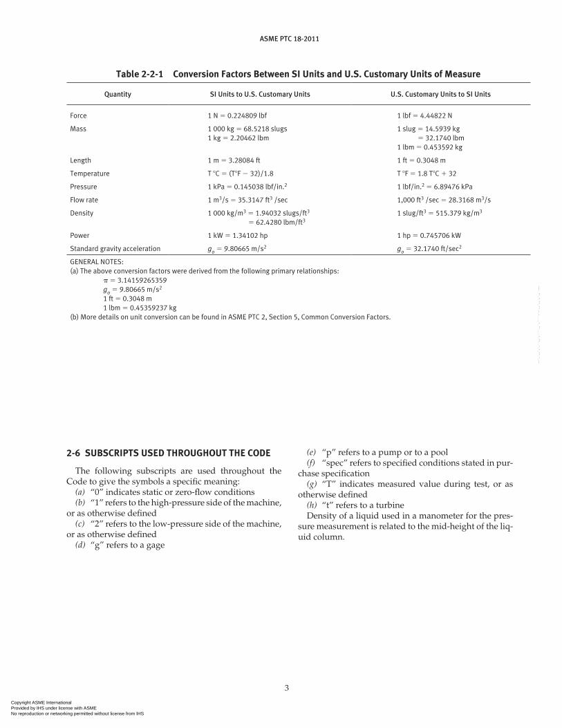
The International System of Units (SI) is used throughout this Code with U.S. Customary Units shown in parentheses (see Table 2-2-1). ASME PTC 2 provides conversion factors for use with ASME per-formance tests.

2-3 TABlES ANd FIGURES

The symbols, terms, definitions, and units in this Code are listed in Tables 2-3-1 through 2-3-8. See Figs. 2-3-1 through 2-3-5 for a graphical definition of certain terms.

2-4 REFERENCE ElEVATION, ZC

By agreement between the parties to the test, the run-ner reference elevation, ZC, for determining the plant cavitation factor may be selected at the location where the development of cavitation has a predominant influ-ence on the performance of the machine. In the absence of such agreement, the reference elevation, ZC, shall be as shown in Fig. 2-4-1.

2-5 CENTRIFUGAl PUmPS

Some definitions in this Code may differ from those customarily associated with centrifugal pumps.


--`,`,,`,`,``,,`,````,,`,````-`-`,,`,,`,`,,`---

ASME PTC 18-2011

3

2-6 SUBSCRIPTS USEd THROUGHOUT THE COdE

The following subscripts are used throughout the Code to give the symbols a specific meaning:

(a) “0” indicates static or zero-flow conditions(b) “1” refers to the high-pressure side of the machine,

or as otherwise defined(c) “2” refers to the low-pressure side of the machine,

or as otherwise defined(d) “g” refers to a gage

(e) “p” refers to a pump or to a pool(f) “spec” refers to specified conditions stated in pur-

chase specification(g) “T” indicates measured value during test, or as

otherwise defined(h) “t” refers to a turbineDensity of a liquid used in a manometer for the pres-

sure measurement is related to the mid-height of the liq-uid column.

Table 2-2-1 Conversion Factors Between SI Units and U.S. Customary Units of measure

Quantity SI Units to U.S. Customary Units U.S. Customary Units to SI Units

Force 1 N 5 0.224809 lbf 1 lbf 5 4.44822 N

Mass 1 000 kg 5 68.5218 slugs1 kg 5 2.20462 lbm

1 slug 5 14.5939 kg5 32.1740 lbm

1 lbm 5 0.453592 kg

Length 1 m 5 3.28084 ft 1 ft 5 0.3048 m

Temperature T 8C 5 (T8F 2 32)/1.8 T 8F 5 1.8 T8C 1 32

Pressure 1 kPa 5 0.145038 lbf/in.2 1 lbf/in.2 5 6.89476 kPa

Flow rate 1 m3/s 5 35.3147 ft3 /sec 1,000 ft3 /sec 5 28.3168 m3/s

Density 1 000 kg/m3 5 1.94032 slugs/ft3

5 62.4280 lbm/ft31 slug/ft3 5 515.379 kg/m3

Power 1 kW 5 1.34102 hp 1 hp 5 0.745706 kW

Standard gravity acceleration go 5 9.80665 m/s2 go 5 32.1740 ft/sec2

GENERAL NOTES:(a) The above conversion factors were derived from the following primary relationships: p 5 3.14159265359 go 5 9.80665 m/s2 1 ft 5 0.3048 m 1 lbm 5 0.45359237 kg(b) More details on unit conversion can be found in ASME PTC 2, Section 5, Common Conversion Factors.


--`,`,,`,`,``,,`,````,,`,````-`-`,,`,,`,`,,`---

ASME PTC 18-2011

4

Table 2-3-1 letter Symbols and definitions

Symbol TermDefinition/Formula/ Reference/Remark

Units

SIU.S.

Customary

A Flow section area Area of water passage cross section normal to general direction of flow

Area of current metering section

m2

m2

ft2

ft2

A1 Area of high-pressure section Area of agreed flow section in machine high-pressure passage between machine and any valve

m2 ft2

A2 Area of low-pressure section Area of agreed flow section in machine low-pressure passage between machine and any valve

m2 ft2

B Width of rectangular conduit section Ultrasonic m ft

Height of distributor Power measurement m ft

Width of impulse turbine bucket Power measurement m ft

Bh Blade height at hub of propeller-type runner Power measurement m ft

Bt Blade height at peripheral of propeller-type runner Power measurement m ft

C1 Concentration of injected dye Dye dilution … …

C2 Dye concentration after complete mixing with flow Dye dilution … …

Co Background dye concentration Dye dilution … …

c Speed of sound in water Ultrasonic m/s ft/sec

D Machine reference diameter Pelton: Pitch diameterKaplan: Discharge ring diameter at center line

of runner bladesFrancis: Runner throat or discharge diameter

m ft

Average diameter in the pressure–time measuring section

Pressure–time m ft

Height of rectangular conduit section Ultrasonic m ft

Di i th diameter measured in a plane in the ultrasonic flow section

Ultrasonic m ft

Ds Dilution factor of standard Dye dilution … …

Dt Dilution factor of test water Dye dilution … …

d Inside diameter of pressure tap Pressure taps m ft

di Tip diameter of the i th current meter Current meters m ft

Distance of the i th chordal path from conduit centerline

Ultrasonic m ft

E Sign factor for direction of acoustic pulse Ultrasonic … …

F Force … N lbf

Pipe factor Pressure–time m21 ft21

Fc Fluorescence corrected to reference temperature Dye dilution … …

Fm Measured fluorescence at sample temperature Dye dilution … …


--`,`,,`,`,``,,`,````,,`,````-`-`,,`,,`,`,,`---

ASME PTC 18-2011

5



Units

SIU.S.

Customary

Fs Fluorescence of standard Dye dilution … …

Ft Fluorescence of test sample Dye dilution … …

FtMean fluorescence of n samples Dye dilution … …

f Pipe friction factor Pressure–time … …

g Local gravitational acceleration Value of acceleration due to gravity at a given geographical location. (See Tables 2-3-2M and 2-3-2)

m/s2 ft/sec2

H Total head Sum of potential, pressure, and velocity heads at given point in the water passage. H 5 Z 1 h 1 hv

m ft

H1 Total head of high-pressure section Sum of potential, pressure, and velocity heads at machine high-pressure section. H1 5 Z1 1 h1 1 hv1

m ft

H2 Total head of low-pressure section Sum of potential, pressure, and velocity heads at machine low-pressure section. H2 5 Z2 1 h2 1 hv2

m ft

HG Gross head Water elevation difference between upper pool and lower pool. HG 5 Z1p 2 Z2p 5 HWL 2 TWL

m ft

HL Head loss Total head loss between any two sections of water passage.

m ft

HL1 Head loss on high-pressure side Head loss between machine and upper pool, including entrance/exit, trashrack, conduit, and valve losses. HL1 5 Z1p 2 H1

m ft

HL2 Head loss on low-pressure side Head loss between machine and lower pool, including entrance/exit, trashrack, conduit, and valve loss. HL2 5 H2 2 Z2p

m ft

HN Net head Difference between total head of high-pressure section and total head of low-pressure section corrected for buoyancy of water in air. HN 5 (Z1 1 h1 2 Z2 2 h2) [1 2 (a/)] 1 hv1 2 hv2

m ft

Hspec Specified head Allowable deviations m ft

HT Net head at test conditions Allowable deviations m ft

HWL Headwater level Z1p relative to the mean sea level

NOTE: An engineering judgment is necessary to determine whether the effect of flow in the pool on its elevation is negligible or whether a correction is needed.

m ft

h Pressure head Height of water column under prevailing condi-tions equivalent to static pressure at given point in the water passage. h 5 p /[g ( 2 a)]

m ft

h1 Pressure head at high-pressure section Height of water column under prevailing conditions equivalent to gage pressure at horizontal centerline of machine high-pressure section, A1. h1 5 p1 /[g ( 2 a)]

m ft

(Cont'd)


--`,`,,`,`,``,,`,````,,`,````-`-`,,`,,`,`,,`---

ASME PTC 18-2011

6



Units

SIU.S.

Customary

h2 Pressure head at low-pressure section Height of water column under prevailing condi-tions equivalent to gage pressure at horizontal centerline of machine low-pressure section, A2. h2 5 p2 /[g ( 2 a)]

m ft

ha Barometric pressure head Height of water column under prevailing conditions equivalent to atmospheric pressure (absolute) at given latitude and elevation. ha 5 pa /[g ( 2 a)]

m ft

hf Average pressure differential in the static line portion of a pressure–time trace corrected for instrument offset


hi Average pressure differential in the running line portion of a pressure–time trace corrected for instrument offset


hm Measured pressure differential between pressure–time sections


hmf Measured average static line pressure differential between pressure–time sections


hmi Measured average running line pressure differential between pressure–time sections


ho Pressure differential between pressure–time sections corrected for instrument offset


hv Velocity head Height of water column under prevailing conditions equivalent to kinetic pressure head in a given flow section. hv 5 v2/2g

m ft

hvp Vapor pressure head Height of water column equivalent to vapor pressure (absolute) of water at temperature of turbine discharge or pump inlet.

m ft

K Shape factor Ultrasonic … …

Differential (Winter–Kennedy) flowmeter coefficient Index testing … …

kf Constant in windage and friction calculation for Francis turbine

Power measurement … …

ki Constant in windage and friction calculation for impulse turbine


kp Constant in windage and friction calculation for propeller turbine


L Length … m ft

Average distance between the pressure–time tap planes


Distance between two ultrasonic transducers Ultrasonic m ft

Li Distance between transducer faces along the i th chordal path

Ultrasonic m ft

Lwi Distance across conduit along the i th chordal path Ultrasonic m ft

M Mass … kg slug

Np Number of blades for a propeller-type runner Power measurement … …

(Cont'd)


--`,`,,`,`,``,,`,````,,`,````-`-`,,`,,`,`,,`---

ASME PTC 18-2011

7



Units

SIU.S.

Customary

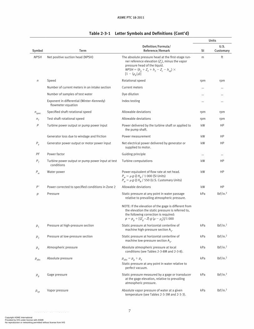
NPSH Net positive suction head (NPSH) The absolute pressure head at the first-stage run-ner reference elevation (Zc), minus the vapor pressure head of the liquid. NPSH 5 (ha 1 Z2 1 h2 2 Zc 2 hvp) 3 [1 2 (a/)]

m ft

n Speed Rotational speed rpm rpm

Number of current meters in an intake section Current meters … …

Number of samples of test water Dye dilution … …

Exponent in differential (Winter–Kennedy) flowmeter equation

Index testing … …

nspec Specified shaft rotational speed Allowable deviations rpm rpm

nT Test shaft rotational speed Allowable deviations rpm rpm

P Turbine power output or pump power input Power delivered by the turbine shaft or applied to the pump shaft.

kW HP

Generator loss due to windage and friction Power measurement kW HP

Pe Generator power output or motor power input Net electrical power delivered by generator or supplied to motor.

kW HP

PF Power factor Guiding principle … …

PT Turbine power output or pump power input at test conditions

Turbine computations kW HP

Pw Water power Power equivalent of flow rate at net head.Pw 5 g Q HN / 1 000 (SI Units)Pw 5 g Q HN / 550 (U.S. Customary Units)

kW HP

P' Power corrected to specified conditions in Zone 2 Allowable deviations kW HP

p Pressure Static pressure at any point in water passage relative to prevailing atmospheric pressure.

NOTE: If the elevation of the gage is different from the elevation the static pressure is referred to, the following correction is required: p 5 pg 1 [(Zg – Z) g ( 2 a)]/1 000

kPa lbf/in.2

p1 Pressure at high-pressure section Static pressure at horizontal centerline of machine high-pressure section A1.

kPa lbf/in.2

p2 Pressure at low-pressure section Static pressure at horizontal centerline of machine low-pressure section A2.

kPa lbf/in.2

pa Atmospheric pressure Absolute atmospheric pressure at local conditions (see Tables 2-3-8M and 2-3-8).

kPa lbf/in.2

pabs Absolute pressure pabs 5 pg 1 pa

Static pressure at any point in water relative to perfect vacuum.

kPa lbf/in.2

pg Gage pressure Static pressure measured by a gage or transducer at the gage elevation, relative to prevailing atmospheric pressure.

kPa lbf/in.2

pvp Vapor pressure Absolute vapor pressure of water at a given temperature (see Tables 2-3-3M and 2-3-3).

kPa lbf/in.2

(Cont'd)


--`,`,,`,`,``,,`,````,,`,````-`-`,,`,,`,`,,`---

ASME PTC 18-2011

8



Units

SIU.S.

Customary

Q Flow rate Volume of water passing through the machine per unit time, including water for seals and thrust relief but excluding water supplied for the operation of auxiliaries and the cooling of all bearings.

m3/s ft3/sec

Q' Flow corrected to specified conditions in Zone 2 Allowable deviations m3/s ft3/sec

Qf Leakage flow rate Pressure–time m3/s ft3/sec

Qi Indicated flow rate from Winter–Kennedy flowmeter

Index testing m3/s ft3/sec

Qm Integrated current-meter flow rate before correction for blockage

Current meters m3/s ft3/sec

Qrel Relative flow rate Index testing m3/s ft3/sec

QT Flow rate at test conditions Allowable deviations m3/s ft3/sec

q Injection rate of dye Dye dilution m3/s ft3/sec

S Frontal area of current-meter support structure Current meters m2 ft2

Standard deviation of fluorescence of n samples Dye dilution … …

Sm Frontal area of current-meter propellers Current meters m2 ft2

T Temperature … 8C 8F

Tr Reference temperature Dye dilution 8C 8F

Ts Temperature of sample water Dye dilution 8C 8F

TWL Tailwater level Z2p relative to the mean sea level

NOTE: An engineering judgment is necessary to determine whether the effect of flow in the pool on its elevation is negligible or whether a correction is needed.

m ft

t Time … s sec

td Downstream transit time of an ultrasonic pulse Ultrasonic s sec

tf Time at the end of the pressure–time integration interval

Pressure–time s sec

ti Time at the start of the pressure–time integration interval

Pressure–time s sec

tn21 Student’s t-statistic for 95% confidence Dye dilution … …

tu Upstream transit time of an ultrasonic pulse Ultrasonic s sec

u Velocity of the runner at diameter, Du 5 5

D Dn

2 60

π m/s ft/sec

(Cont'd)


--`,`,,`,`,``,,`,````,,`,````-`-`,,`,,`,`,,`---

ASME PTC 18-2011

9



Units

SIU.S.

Customary

V Mean axial component of water velocity over a chordal path

Ultrasonic m/s ft/sec

Vc Mean transverse component of velocity over a chordal path

Ultrasonic m/s ft/sec

Vi Average velocity along the i th chordal path Ultrasonic m/s ft/sec

v Mean velocity Flow rate divided by flow-section area. m/s ft/sec

v1 Mean velocity at high-pressure section Flow rate divided by high-pressure flow section area.

m/s ft/sec

v2 Mean velocity at low-pressure section Flow rate divided by low-pressure flow section area.

m/s ft/sec

Wi Weighting factor for the i th chordal path Ultrasonic … …

Wi' Modified weighting factor along the i th chordal path Ultrasonic … …

Y Sign factor for transverse velocity component Ultrasonic … …

Z Potential head Elevation of a measurement point relative to a common datum.

m ft

Z1 Potential head at high-pressure section Elevation of horizontal centerline of machine high-pressure section relative to a common datum.

m ft

Z1p Potential head of upper pool Elevation of upper pool relative to a common datum. Also see “Headwater level.”

m ft

Z2 Potential head at low-pressure section Elevation of horizontal centerline of machine low-pressure section relative to a common datum.

m ft

Z2p Potential head of lower pool Elevation of lower pool relative to a common datum. Also see “Tailwater level.”

m ft

Zc Potential head at runner reference elevation Elevation of cavitation reference location relative to a common datum. (Fig. 2-4-1)

m ft

Zg Potential head at gage elevation Elevation of a pressure gage typically used to measure pg (Figs. 2-3-1 through 2-3-5).

m ft

Angular location of Winter–Kennedy taps in spiral case

Index testing deg deg

H Pump head correction to specified conditions Pump computations m ft

h Flowmeter differential pressure Index testing kPa lbf/in.2

P Pump power correction to specified conditions Pump computations kW HP

Q Pump flow correction to specified conditions Pump computations m3/s ft3/sec

Efficiency Turbine: P/PW, Pump: PW/P … …

Density of water Mass per unit volume of water at measured temperature and pressure (see Table 2-3-5).

kg/m3 slugs/ ft3

a Density of dry air Mass per unit volume of ambient air at measured temperature and barometric pressure (see Tables 2-3-6M and 2-3-6).

kg/m3 slugs/ ft3

(Cont'd)


--`,`,,`,`,``,,`,````,,`,````-`-`,,`,,`,`,,`---

ASME PTC 18-2011

10



Units

SIU.S.

Customary

Hg Density of mercury Mass per unit volume of mercury at measured temperature and barometric pressure (see Tables 2-3-7M and 2-3-7).

kg/m3 slugs/ ft3

Cavitation factor NPSH

H5 … …

Angle between acoustic path and direction of water flow

Ultrasonic deg deg

Angular speed Radians per second rad/s rad/sec

GENERAL NOTES:(a) See Figs. 2-3-1 through 2-3-5.(b) The following subscripts are used to give the symbols a specific meaning:

(1) “0” indicates static or zero flow conditions.(2) “1” refers to the high pressure side of the machine, or as otherwise defined.(3) “2” refers to the low pressure side of the machine, or as otherwise defined.(4) “g” refers to a gage.(5) “p” refers to a pump or to a pool.(6) “spec” refers to specified conditions stated in purchase specification.(7) “T” indicates measured value during test, or as otherwise defined.(8) “t” refers to a turbine. Density of a liquid used in a manometer for the pressure measurement is related to the mid-height of the liquid column.

(Cont'd)

Table 2-3-2m Acceleration of Gravity as a Function of latitude and Elevation, SI Units (m/s2)

Latitude, (deg)

Altitude Above Mean Sea Level, Z, m

0 500 1 000 1 500 2 000 2 500 3 000 3 500

0 9.78036 9.77881 9.77727 9.77573 9.77418 9.77264 9.77110 9.76956

10 9.78191 9.78037 9.77882 9.77728 9.77574 9.77419 9.77265 9.77111

20 9.78638 9.78484 9.78330 9.78175 9.78021 9.77867 9.77712 9.77558

30 9.79324 9.79170 9.79016 9.78861 9.78707 9.78553 9.78399 9.78244

40 9.80167 9.80013 9.79858 9.79704 9.79550 9.79396 9.79241 9.79087

50 9.81065 9.80911 9.80757 9.80602 9.80448 9.80294 9.80139 9.79985

60 9.81911 9.81756 9.81602 9.81448 9.81293 9.81139 9.80985 9.80830

70 9.82601 9.82446 9.82292 9.82138 9.81983 9.81829 9.81675 9.81520

80 9.83051 9.82897 9.82743 9.82588 9.82434 9.82280 9.82126 9.81971

90 9.83208 9.83054 9.82899 9.82745 9.82591 9.82436 9.82282 9.82128


--`,`,,`,`,``,,`,````,,`,````-`-`,,`,,`,`,,`---

ASME PTC 18-2011

11

Table 2-3-2 Acceleration of Gravity as a Function of latitude and Elevation, U.S. Customary Units (ft/sec2)

Latitude, Altitude Above Mean Sea Level, Z, ft

(deg) 0 2,000 4,000 6,000 8,000 10,000 12,000

0 32.0878 32.0816 32.0754 32.0693 32.0631 32.0569 32.0508

10 32.0929 32.0867 32.0805 32.0744 32.0682 32.0620 32.0558

20 32.1076 32.1014 32.0952 32.0890 32.0829 32.0767 32.0705

30 32.1301 32.1239 32.1177 32.1115 32.1054 32.0992 32.0930

40 32.1577 32.1515 32.1454 32.1392 32.1330 32.1269 32.1207

50 32.1872 32.1810 32.1748 32.1687 32.1625 32.1563 32.1501

60 32.2149 32.2087 32.2026 32.1964 32.1902 32.1841 32.1779

70 32.2375 32.2314 32.2252 32.2190 32.2129 32.2067 32.2005

80 32.2523 32.2462 32.2400 32.2338 32.2277 32.2215 32.2153

90 32.2575 32.2513 32.2451 32.2390 32.2328 32.2266 32.2204

GENERAL NOTES:(a) Reference: Lide, D.R., Editor, CRC Handbook of Chemistry and Physics, 90th Edition, CRC Press, New York, 2009. (b) Gravitational acceleration formula given in the reference noted in (a) above:

g 5 9.780356(1 1 0.0052885 sin2 2 2 0.0000059 sin2 2)2 3.086 3 1026 Z

where acceleration g is in m/s2, latitude is in degrees, and elevation Z is in meters.(c) Conversion to U.S. Customary units: g (ft/sec2) 5 g (m/s2)/0.3048(d) The standard value of gravitational acceleration adopted by the International Bureau of Weights and Measures is g 5 9.80665 m/s2

or 32.17405 ft/s2.

Table 2-3-3m Vapor Pressure of distilled Water as a Function of Temperature, SI Units (kPa)

Temperature T, 8C

Vapor Pressure, pvp, kPa

Temperature T, 8C


0 0.6112 … …

1 0.6571 21 2.488

2 0.7060 22 2.645

3 0.7581 23 2.811

4 0.8135 24 2.986

5 0.8726 25 3.170

6 0.9354 26 3.364

7 1.002 27 3.568

8 1.073 28 3.783

9 1.148 29 4.009

10 1.228 30 4.247

11 1.313 31 4.497

12 1.403 32 4.759

13 1.498 33 5.035

14 1.599 34 5.325

15 1.706 35 5.629

16 1.819 36 5.947

17 1.938 37 6.282


--`,`,,`,`,``,,`,````,,`,````-`-`,,`,,`,`,,`---

ASME PTC 18-2011

12

Table 2-3-3m Vapor Pressure of distilled Water as a Function of Temperature, SI Units (kPa)

Temperature T, 8C


Temperature T, 8C


18 2.065 38 6.632

19 2.198 39 7.000

20 2.339 40 7.384

GENERAL NOTES:(a) Reference: Parry, W.T., et al, ASME International Steam Tables, 2nd Edition,

American Society of Mechanical Engineers, New York, 2009.(b) The vapor pressure of water can be calculated between the temperatures

0 , T , 408C using the following empirical equation:

pvp 5 102.7862 1 0.0312 T 20.000104 T2

with an error smaller than 0.009 kPa.(c) Conversion factors to U.S. Customary Units

T (8F) 5 T(8C) 3 1.8 1 32pvp (lbf/in.2) 5 pvp (kPa) 3 1000 3 (0.3048/12)2/0.45359237/9.80665

Table 2-3-3 Vapor Pressure of distilled Water as a Function of Temperature, U.S. Customary Units (lbf/in.2)

Temperature, T, 8F

Vapor Pressure, pvp, lbf/in.2

Temperature, T, 8F

Vapor Pressure, pvp, lbf/in.2

32 0.08865 … …

34 0.09607 74 0.41599

36 0.10403 76 0.44473

38 0.11258 78 0.47518

40 0.12173 80 0.50744

42 0.13155 82 0.54159

44 0.14205 84 0.57772

46 0.15328 86 0.61593

48 0.16530 88 0.65632

50 0.17813 90 0.69899

52 0.19184 92 0.74405

54 0.20646 94 0.79161

56 0.22206 96 0.84178

58 0.23868 98 0.89468

60 0.25639 100 0.95044

62 0.27524 102 1.0092

64 0.29529 104 1.0710

66 0.31662 106 1.1361

68 0.33927 108 1.2046

70 0.36334 110 1.2766

72 0.38889 112 1.3523


American Society of Mechanical Engineers, New York, 2009.(b) The vapor pressure of water can be calculated between the temperatures

0 , T , 408C using the following empirical equation:

pvp 5 102.7862 1 0.0312 T 20.000104 T2

with an error smaller than 0.009 kPa.(c) Conversion factors to U.S. Customary Units

T (8F) 5 T(8C) 3 1.8 1 32pvp (lbf/in.2) 5 pvp (kPa) 3 1000 3 (0.3048/12)2/0.45359237/9.80665

(Cont'd)


--`,`,,`,`,``,,`,````,,`,````-`-`,,`,,`,`,,`---

ASME PTC 18-2011

13

Table 2-3-4m density of Water as a Function of Temperature and Pressure, SI Units (kg/m3)

Temperature, T, 8C

Absolute Pressure, pabs, kPa

100 101.325 500 1 000 2 000 3 000 4 000 5 000 10 000 15 000

0 999.85 999.85 1 000.05 1 000.30 1 000.81 1 001.32 1 001.82 1 002.32 1 004.82 1 007.30

1 999.90 999.90 1 000.11 1 000.36 1 000.86 1 001.36 1 001.86 1 002.36 1 004.85 1 007.30

2 999.94 999.95 1 000.15 1 000.40 1 000.90 1 001.39 1 001.89 1 002.39 1 004.85 1 007.29

3 999.97 999.97 1 000.17 1 000.42 1 000.91 1 001.41 1 001.90 1 002.40 1 004.85 1 007.27

4 999.98 999.98 1 000.17 1 000.42 1 000.91 1 001.41 1 001.90 1 002.39 1 004.82 1 007.23

5 999.97 999.97 1 000.16 1 000.41 1 000.90 1 001.39 1 001.88 1 002.36 1 004.78 1 007.17

6 999.94 999.94 1 000.14 1 000.38 1 000.87 1 001.36 1 001.84 1 002.33 1 004.73 1 007.11

7 999.90 999.91 1 000.10 1 000.34 1 000.83 1 001.31 1 001.79 1 002.27 1 004.66 1 007.03

8 999.85 999.85 1 000.04 1 000.29 1 000.77 1 001.25 1 001.73 1 002.21 1 004.58 1 006.93

9 999.78 999.78 999.98 1 000.22 1 000.69 1 001.17 1 001.65 1 002.13 1 004.49 1 006.83

10 999.70 999.70 999.89 1 000.13 1 000.61 1 001.08 1 001.56 1 002.03 1 004.38 1 006.71

12 999.50 999.50 999.69 999.93 1 000.40 1 000.87 1 001.34 1 001.81 1 004.13 1 006.44

14 999.25 999.25 999.43 999.67 1 000.14 1 000.60 1 001.07 1 001.53 1 003.84 1 006.12

16 998.95 998.95 999.13 999.36 999.83 1 000.29 1 000.75 1 001.21 1 003.50 1 005.76

18 998.60 998.60 998.78 999.01 999.47 999.93 1 000.39 1 000.85 1 003.11 1 005.36

20 998.21 998.21 998.39 998.62 999.07 999.53 999.98 1 000.44 1 002.69 1 004.92

22 997.77 997.77 997.96 998.18 998.64 999.09 999.54 999.99 1 002.23 1 004.44

24 997.30 997.30 997.48 997.71 998.16 998.61 999.05 999.50 1 001.73 1 003.93

26 996.79 996.79 996.97 997.19 997.64 998.09 998.53 998.98 1 001.19 1 003.38

28 996.24 996.24 996.42 996.64 997.09 997.53 997.97 998.42 1 000.62 1 002.80

30 995.65 995.65 995.83 996.05 996.50 996.94 997.38 997.82 1 000.01 1 002.18

32 995.03 995.03 995.21 995.43 995.87 996.31 996.75 997.19 999.37 1 001.54

34 994.38 994.38 994.56 994.78 995.22 995.66 996.09 996.53 998.71 1 000.86

36 993.69 993.69 993.87 994.09 994.53 994.96 995.40 995.84 998.00 1 000.15

38 992.98 992.98 993.15 993.37 993.81 994.24 994.68 995.11 997.27 999.41

40 992.23 992.23 992.40 992.62 993.06 993.49 993.93 994.36 996.52 998.65

GENERAL NOTES:(a) The densities given above were computed from the following equation:

� ��

� ��

�

�

�

p

R Tn I

p

p

T

Ti i

Ii*

( . ) ).

*

*

( ..

273 157 1

273 151 222

1

∑J

i

i�

1

181

where 5 density of water (kg/m3)T 5 water temperature (8C)p 5 absolute pressure (kPa)

constants:p*5 16,530 kPaT*5 1,386 KR 5 0.461526 kJ/kg · K

Refer to Table 2-3-5 for coefficients Ii, Ji, and ni.(b) Intermediate values may be interpolated or calculated from the equation given in in General Note (a).(c) The values in this table were computed from the equation in General Note (a), using the following conversion factors:

T (8F) 5 T (8C) 3 1.8 1 32pabs (lbf/in.2) 5 pabs (kPa) 3 1,000 3 (0.3048/12)2/0.45359237/9.80665 (slug/ft3) 5 (kg/m3) 3 (0.3048)4/0.45359237/9.80665

(d) Standard atmospheric pressure is 101.325 kPa (refer to Tables 2-3-8M and 2-3-8).


--`,`,,`,`,``,,`,````,,`,````-`-`,,`,,`,`,,`---

ASME PTC 18-2011

14

Table 2-3-4 density of Water as a Function of Temperature and Pressure, U.S. Customary Units (slug/ft3)

Temperature, T, 8F

Pressure, pabs, lbf/in.2

14 14.696 15 25 50 100 200 500 1,000 2,000

32 1.94002 1.94002 1.94003 1.94009 1.94026 1.94060 1.94128 1.94331 1.94668 1.95333

34 1.94014 1.94015 1.94015 1.94022 1.94039 1.94072 1.94140 1.94341 1.94675 1.95334

36 1.94023 1.94023 1.94023 1.94030 1.94047 1.94080 1.94147 1.94347 1.94678 1.95333

38 1.94027 1.94027 1.94027 1.94034 1.94051 1.94084 1.94150 1.94349 1.94677 1.95327

40 1.94027 1.94028 1.94028 1.94034 1.94051 1.94084 1.94150 1.94347 1.94673 1.95318

42 1.94024 1.94024 1.94024 1.94031 1.94047 1.94080 1.94145 1.94341 1.94665 1.95306

44 1.94016 1.94017 1.94017 1.94024 1.94040 1.94072 1.94137 1.94332 1.94654 1.95291

46 1.94006 1.94006 1.94006 1.94013 1.94029 1.94061 1.94126 1.94319 1.94639 1.95272

48 1.93992 1.93992 1.93992 1.93999 1.94015 1.94047 1.94111 1.94303 1.94621 1.95250

50 1.93974 1.93975 1.93975 1.93981 1.93997 1.94029 1.94093 1.94284 1.94600 1.95225

55 1.93917 1.93918 1.93918 1.93924 1.93940 1.93971 1.94034 1.94222 1.94534 1.95151

60 1.93841 1.93842 1.93842 1.93848 1.93864 1.93895 1.93957 1.94143 1.94451 1.95061

65 1.93748 1.93748 1.93749 1.93755 1.93770 1.93801 1.93862 1.94046 1.94351 1.94954

70 1.93639 1.93639 1.93639 1.93645 1.93660 1.93691 1.93752 1.93934 1.94236 1.94833

75 1.93514 1.93514 1.93514 1.93520 1.93535 1.93566 1.93626 1.93806 1.94105 1.94697

80 1.93374 1.93375 1.93375 1.93381 1.93396 1.93426 1.93486 1.93665 1.93961 1.94549

85 1.93221 1.93221 1.93222 1.93228 1.93242 1.93272 1.93332 1.93509 1.93804 1.94388

90 1.93055 1.93055 1.93055 1.93061 1.93076 1.93106 1.93165 1.93341 1.93635 1.94215

95 1.92876 1.92876 1.92876 1.92882 1.92897 1.92926 1.92985 1.93161 1.93453 1.94030

100 1.92685 1.92685 1.92685 1.92691 1.92706 1.92735 1.92794 1.92969 1.93260 1.93835

105 1.92482 1.92483 1.92483 1.92489 1.92503 1.92533 1.92591 1.92766 1.93055 1.93628

110 1.92269 1.92269 1.92269 1.92275 1.92290 1.92319 1.92377 1.92551 1.92840 1.93412

GENERAL NOTES:(a) The densities given above were computed from the following equation:

� ��

� ��

�

�

�

p

R Tn I

p

p

T

Ti i

Ii*

( . ) ).

*

*

( ..

273 157 1

273 151 222

1

∑J

i

i�

1

181

where 5 density of water (kg/m3)T 5 water temperature (8C)p 5 absolute pressure (kPa)

constants:p* 5 16,530 kPa T* 5 1,386 K R 5 0.461526 kJ/kg · K

Refer to Table 2-3-5 for coefficients Ii, Ji, and ni.(b) Intermediate values may be interpolated or calculated from the equation given in in General Note (a).(c) The values in this table were computed from the equation in General Note (a), using the following conversion factors:

T (8F) 5 T (8C) 3 1.8 1 32pabs (lbf/in.2) 5 pabs (kPa) 3 1,000 3 (0.3048/12)2/0.45359237/9.80665 (slug/ft3) 5 (kg/m3) 3 (0.3048)4/0.45359237/9.80665

(d) Standard atmospheric pressure is 14.696 lbf/in.2 (refer to Tables 2-3-8M and 2-3-8).


--`,`,,`,`,``,,`,````,,`,````-`-`,,`,,`,`,,`---

ASME PTC 18-2011

15

Table 2-3-5 Coefficients Ii, Ji, and ni

i Ii Ji ni

1 1 21 21.89900E-02

2 1 0 23.25297E-02

3 1 1 22.18417E-02

4 1 3 25.28383E-05

5 2 23 24.71843E-04

6 2 0 23.00017E-04

7 2 1 4.76613E-05

8 2 3 24.41418E-06

9 2 17 27.26949E-16

10 3 24 23.16796E-05

11 3 0 22.82707E-06

12 3 6 28.52051E-10

13 4 25 22.24252E-06

14 4 22 26.51712E-07

15 4 10 21.43417E-13

16 5 28 24.05169E-07

17 8 211 21.27343E-09

18 8 26 21.74248E-10


American Society of Mechanical Engineers, New York, 2009.(b) The referenced ASME steam tables are based on the IAPSW Industrial

Formulation 1997.(c) The above coefficients are a subset of the full Region 1 formulation defined

in the reference, and yield densities within 0.01 kg/m3 ( 0.001%) of the full formulation in the range 0 , T , 70 8C and 0.5 , p , 20,000 kPa.


--`,`,,`,`,``,,`,````,,`,````-`-`,,`,,`,`,,`---

ASME PTC 18-2011

16

Table 2-3-6m density of dry Air, SI Units (kg/m3)

Altitude, Z, m

Temperature, T, 8C

220 210 0 10 15 20 30 40 50

0 1.3944 1.3414 1.2923 1.2466 1.2250 1.2041 1.1644 1.1272 1.0923

500 1.3137 1.2637 1.2175 1.1745 1.1541 1.1344 1.0970 1.0620 1.0291

1 000 1.2368 1.1898 1.1462 1.1058 1.0866 1.0680 1.0328 0.9998 0.9689

1 500 1.1636 1.1194 1.0784 1.0403 1.0223 1.0048 0.9717 0.9407 0.9115

2 000 1.0940 1.0524 1.0139 0.9780 0.9611 0.9447 0.9135 0.8844 0.8570

2 500 1.0277 0.9887 0.9525 0.9188 0.9029 0.8875 0.8582 0.8308 0.8051

3 000 0.9648 0.9281 0.8941 0.8626 0.8476 0.8331 0.8057 0.7799 0.7558

3 500 0.9050 0.8706 0.8387 0.8091 0.7951 0.7815 0.7557 0.7316 0.7090

4 000 0.8482 0.8160 0.7861 0.7584 0.7452 0.7325 0.7083 0.6857 0.6645

GENERAL NOTES:(a) Reference: U.S. Standard Atmosphere, U.S. Government Printing Office, Washington, D.C., 1976. (b) Air density a (kg/m3) at temperature T (8C) and elevation Z (m) is computed from the U.S. Standard Atmosphere 1976 formulation for

pressure, using the ideal gas law to account for the effect of temperature

(�a TZ�

��

352 9838

273 151 2 2558 10 5 5 2559.

..

.)The use of the geometric elevation Z instead of the geopotential elevation specified in the reference produces densities accurate to within 0.033%.

(c) Conversion factor: a (slug/ft3) 5 a (kg/m3) 3 (0.3048)4/0.45359237/9.80665

Table 2-3-6 density of dry Air, U.S. Customary Units (slug/ft3)

Altitude, Z, ft

Temperature, T, 8F

0 20 40 60 80 100 120

0 0.002682 0.002570 0.002467 0.002372 0.002284 0.002203 0.002127

1,000 0.002586 0.002479 0.002379 0.002288 0.002203 0.002124 0.002051

2,000 0.002494 0.002390 0.002294 0.002206 0.002124 0.002048 0.001977

3,000 0.002404 0.002303 0.002211 0.002126 0.002047 0.001974 0.001906

4,000 0.002316 0.002220 0.002131 0.002049 0.001973 0.001902 0.001837

5,000 0.002232 0.002138 0.002053 0.001974 0.001901 0.001833 0.001770

6,000 0.002149 0.002060 0.001977 0.001901 0.001831 0.001765 0.001704

7,000 0.002069 0.001983 0.001904 0.001831 0.001763 0.001700 0.001641

8,000 0.001992 0.001909 0.001833 0.001762 0.001697 0.001636 0.001580

9,000 0.001917 0.001837 0.001764 0.001696 0.001633 0.001575 0.001520

10,000 0.001844 0.001767 0.001697 0.001631 0.001571 0.001515 0.001463

11,000 0.001774 0.001700 0.001632 0.001569 0.001511 0.001457 0.001407

12,000 0.001706 0.001635 0.001569 0.001509 0.001453 0.001401 0.001353

GENERAL NOTES:(a) Reference: U.S. Standard Atmosphere, U.S. Government Printing Office, Washington, D.C., 1976. (b) Air density a (kg/m3) at temperature T (8C) and elevation Z (m) is computed from the U.S. Standard Atmosphere 1976 formulation for

pressure, using the ideal gas law to account for the effect of temperature

(�a TZ�

��

352 9838

273 151 2 2558 10 5 5 2559.

..

.)The use of the geometric elevation Z instead of the geopotential elevation specified in the reference produces densities accurate to within 0.033%.

(c) Conversion factor: a (slug/ft3) 5 a (kg/m3) 3 (0.3048)4/0.45359237/9.80665


--`,`,,`,`,``,,`,````,,`,````-`-`,,`,,`,`,,`---

ASME PTC 18-2011

17

Table 2-3-7m density of mercury, SI Units (kg/m3)

Temperature,8C

Density,kg/m3

Temperature, 8C

Density,kg/m3

210 13,619.8 16 13,555.7

29 13,617.3 17 13,553.3

28 13,614.8 18 13,550.8

27 13,612.4 19 13,548.3

26 13,609.9 20 13,545.9

25 13,607.4 21 13,543.4

24 13,605.0 22 13,541.0

23 13,602.5 23 13,538.5

22 13,600.0 24 13,536.1

21 13,597.6 25 13,533.6

0 13,595.1 26 13,531.2

1 13,592.6 27 13,528.7

2 13,590.2 28 13,526.3

3 13,587.7 29 13,523.8

4 13,585.2 30 13,521.4

5 13,582.8 31 13,518.9

6 13,580.3 32 13,516.5

7 13,577.8 33 13,514.1

8 13,575.4 34 13,511.6

9 13,572.9 35 13,509.2

10 13,570.5 36 13,506.7

11 13,568.0 37 13,504.3

12 13,565.5 38 13,501.8

13 13,563.1 39 13,499.4

14 13,560.6 40 13,497.0

15 13,558.2 … …

GENERAL NOTES:(a) Reference: ASME Fluid Meters, 6th Edition, 1971, Table II-1-2(b) The above table is computed from the equation

5 (851.457 2 0.0859301T 1 6.20046 3 1026T2) 3 0.3048 / 9.80665where density is in slugs/ft3 and temperature T is in degrees Fahrenheit. Computed values agree with the referenced table to within 0.0001%

(c) The above table is computed for atmospheric pressure. At 100 atm, the density of mercury changes by only 0.018%. Therefore, the compressibility of mercury at pressures normally seen in hydraulic machine operations may be neglected.

(d) Conversion factors to U.S. Customary Units:T (8F) 5 T (8C) 3 1.8 1 32 (slugs/ft3) 5 (kg/m3) 3 (0.3048)4/0.45359237/9.80665


--`,`,,`,`,``,,`,````,,`,````-`-`,,`,,`,`,,`---

ASME PTC 18-2011

18

Table 2-3-7 density of mercury, U.S. Customary Units (slugs/ft3)

Temperature,8F

Density,slugs/ft3

Temperature,8F

Density,slugs/ft3

20 26.4108 72 26.2728

22 26.4054 74 26.2675

24 26.4001 76 26.2622

26 26.3948 78 26.2569

28 26.3895 80 26.2517

30 26.3841 82 26.2464

32 26.3788 84 26.2411

34 26.3735 86 26.2358

36 26.3682 88 26.2306

38 26.3629 90 26.2253

40 26.3576 92 26.2200

42 26.3523 94 26.2147

44 26.3470 96 26.2095

46 26.3416 98 26.2042

48 26.3363 100 26.1989

50 26.3310 102 26.1937

52 26.3257 104 26.1884

54 26.3204 106 26.1832

56 26.3151 108 26.1779

58 26.3098 110 26.1726

60 26.3045 … …

62 26.2992 … …

64 26.2940 … …

66 26.2887 … …

68 26.2834 … …

70 26.2781 … …

GENERAL NOTES:(a) Reference: ASME Fluid Meters, 6th Edition, 1971, Table II-1-2(b) The above table is computed from the equation

5 (851.457 2 0.0859301T 1 6.20046 3 1026T2) 3 0.3048 / 9.80665where density is in slugs/ft3 and temperature T is in degrees Fahrenheit. Computed values agree with the referenced table to within 0.0001%

(c) The above table is computed for atmospheric pressure. At 100 atm, the density of mercury changes by only 0.018%. Therefore, the compressibility of mercury at pressures normally seen in hydraulic machine operations may be neglected.

(d) Conversion factors to U.S. Customary Units:T (8F) 5 T (8C) 3 1.8 1 32 (slugs/ft3) 5 (kg/m3) 3 (0.3048)4/0.45359237/9.80665


--`,`,,`,`,``,,`,````,,`,````-`-`,,`,,`,`,,`---

ASME PTC 18-2011

19

Table 2-3-8m Atmospheric Pressure, SI Units (kPa)Altitude, Z, m Atmospheric Pressure, pa, kPa

0 101.325

500 95.461

1 000 89.875

1 500 84.556

2 000 79.495

2 500 74.682

3 000 70.108

3 500 65.764

4 000 61.640

GENERAL NOTES:(a) Reference: U.S. Standard Atmosphere, U.S. Government Printing Office,

Washington, D.C., 1976.(b) Air pressure pa (kPa) at elevation Z (m) is computed from the U.S. Standard

Atmosphere 1976 formulation

pa 5 101.325(1 22.2558 3 1025Z)5.2559

(c) The use of the geometric elevation Z instead of the geopotential elevation specified in the reference produces pressures accurate to within 0.033%.

(d) Conversion factor:pa (lbf/in.2) 5 pa (kPa) 3 1 000 3 (0.3048/12)2/0.45359237/9.80665

Table 2-3-8 Atmospheric Pressure, U.S. Customary Units (lbf/in.2)

Altitude, Z, ft Atmospheric Pressure, pa, lbf/in.2

1,000 14.1726

2,000 13.6644

3,000 13.1711

4,000 12.6923

5,000 12.2277

6,000 11.7770

7,000 11.3398

8,000 10.9159

9,000 10.5048

10,000 10.1064

11,000 9.7204

12,000 9.3463

GENERAL NOTES:(a) Reference: U.S. Standard Atmosphere, U.S. Government Printing Office,

Washington, D.C., 1976.(b) Air pressure pa (kPa) at elevation Z (m) is computed from the U.S. Standard

Atmosphere 1976 formulation

pa 5 101.325(1 22.2558 3 1025z)5.2559

(c) The use of the geometric elevation Z instead of the geopotential elevation specified in the reference produces pressures accurate to within 0.033%.

(d) Conversion factor:pa (lbf/in.2) 5 pa (kPa) 3 1 000 3 (0.3048/12)2/0.45359237/9.80665


--`,`,,`,`,``,,`,````,,`,````-`-`,,`,,`,`,,`---

ASME PTC 18-2011

20

Fig. 2-3-1 Head definition, measurement and Calibration, Vertical Shaft machine With Spiral Case and Pressure Conduit

HWL

Pressure gage, Pg TWLHL2

[No

te (

1)]

HG

hv2

H2 h

2

Zg

Z2

Z2p

V2

Hig

h p

ress

ure

sec

tio

n

Low

pre

ssu

re s

ecti

on

HL1

[No

te (

1)]

hv1

V1

Datum

Z1p

H1

Z1

h1

Density of water by static check using deadweight gage reading pg

p

GENERAL NOTES:(a) Z1p0 (not shown) will be level Z1p at zero flow rate.(b) Z2p0 (not shown) will be level Z2p at zero flow rate.(c) Net head is defined as HH 5 (Z1 1 h1 2Z2 2 h2)(1 2 [a/] ) 1 hv1 2 hv2

NOTE:(1) Head losses, HL1 and HL2 are shown for the turbine mode. For the pump mode, the head losses will be of the opposite sign.


--`,`,,`,`,``,,`,````,,`,````-`-`,,`,,`,`,,`---

ASME PTC 18-2011

21

Fig. 2-3-2 Head definition, measurement and Calibration, Vertical Shaft machine With Semi-Spiral Case

HWLH

L1 [N

ote

(1)

]

hv1

Hig

h p

ress

ure

sec

tio

nPressure gage, Pg

Low

pre

ssu

re s

ecti

on

TWLHL2

[No

te (

1)]

HG

hv2

H2 h

2

Zg

Z2

Z2p

V2

V1

Datum

Z1p

H1

Z1

h1


p


NOTE:(1) Head losses, HL1 and HL2 are shown for the turbine mode. For the pump mode, the head losses will be of the opposite sign.


--`,`,,`,`,``,,`,````,,`,````-`-`,,`,,`,`,,`---

ASME PTC 18-2011

22

Fig. 2-3-3 Head definition, measurement and Calibration, Bulb machine

HWL

HL1

[No

te (

1)]

hv1

Hig

h p

ress

ure

sec

tio

n

Pre

ssu

re g

age,

Pg

Low

pre

ssu

re s

ecti

on

TWLHL2

[ No

te (

1)]

HG

hv2

H2

h2

Zg

Z2 Z

2p

V2

V1

Datum

Z1p

H1

Z1

h1


pg


NOTE:(1) Head losses, HL1 and HL2,are shown for the turbine mode. For the pump mode, the head losses will be of the opposite sign.


--`,`,,`,`,``,,`,````,,`,````-`-`,,`,,`,`,,`---

ASME PTC 18-2011

23

Fig. 2-3-4 Head definition, measurement and Calibration, Horizontal Shaft Impulse Turbine (One or Two Jets)

TWL

hv1

Hig

h p

ress

ure

sec

tio

n

H2 � Z2

Zg

Z1p

Pressure gage, Pg

V1

Datum

Z2p

H1

Z2–

Low

er je

t

Z2–

Bo

th je

ts

Z2–

Up

per

jet

h2 � 0

Z1

HWL HL1

h1


pg

GENERAL NOTES:(a) Z1p0 (not shown) will be level Z1p at zero flow rate.(b) Z2p0 (not shown) will be level Z2p at zero flow rate.(c) Net head is defined as HH 5 (Z1 1 h1 2Z2 2 h2)(1 2 [a/ ] ) 1 hv1 2 hv2


--`,`,,`,`,``,,`,````,,`,````-`-`,,`,,`,`,,`---

ASME PTC 18-2011

24

Fig. 2-3-5 Head definition, measurement and Calibration, Vertical Shaft Impulse Turbine

TWL

hv1

Hig

h p

ress

ure

sec

tio

n

H2 � Z2

Zg

Z2

Pressure gage Pg

V1

Datum Z2p

h2 � 0Z1

HWL HL1

h1

Z1p

H1


pg

GENERAL NOTES:(a) Z1p0 (not shown) will be level Z1p at zero flow rate.(b) Z2p0 (not shown) will be level Z2p at zero flow rate.(c) Net head is defined as HH 5 (Z1 1 h1 2Z2 2 h2)(1 2 [a/ ] ) 1 hv1 2 hv2


--`,`,,`,`,``,,`,````,,`,````-`-`,,`,,`,`,,`---

ASME PTC 18-2011

25

Fig. 2-4-1 Reference Elevation, Zc, of Turbines and Pump-Turbines

Reference datum

α

(a) (b) (c) (d)

(e) (f)

00

ZC

Reference datum

Radial machines, such as Francis turbines and pump–turbines; for multistage machines; low-pressure stage.Diagonal (mixed–flow, semi–axial) machines with fixed runner/impeller blades and with runner/impeller band.Diagonal (mixed–flow, semi–axial) machines with fixed runner/impeller blades without runner/impeller band.

(a)(b)(c)

Diagonal (mixed–flow, semi–axial) machines with adjustable runner/impeller blades.(d)Axial machines, such as propeller turbines and pump–turbines with fixed runner/impeller blades.(e)Axial machines, such as Kaplan turbines and pump–turbines with adjustable runner/impeller blades.(f)

Reference elevation of the machine (ZC)

0 deg � α � 90 deg

00

ZC

Reference elevation of the machine (ZC)

GENERAL NOTE: ASME thanks the International Electrotechnical Commission (IEC) for permission to reproduce information from its International Publication IEC 60041 ed, 3.0 (1991). All such extracts are copyright of IEC, Geneva, Switzerland. All rights reserved. Further information on the IEC is available from www.iec.ch. IEC has no responsibility for the placement and context in which the extracts and contents are reproduced by ASME, nor is IEC in any way responsible for the other content or accuracy therein.IEC 60041 ed. 3.0, Copyright 1991, IEC Geneva, Switzerland www.iec.ch


--`,`,,`,`,``,,`,````,,`,````-`-`,,`,,`,`,,`---

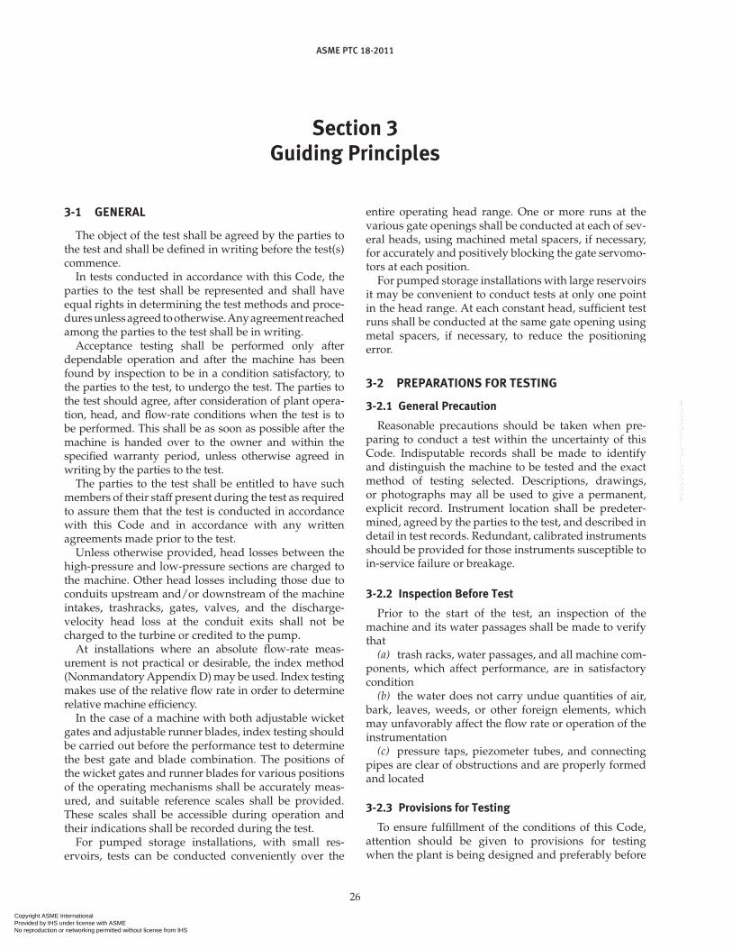
ASME PTC 18-2011

26

3-1 GENERAl

The object of the test shall be agreed by the parties to the test and shall be defined in writing before the test(s) commence.

In tests conducted in accordance with this Code, the parties to the test shall be represented and shall have equal rights in determining the test methods and proce-dures unless agreed to otherwise. Any agreement reached among the parties to the test shall be in writing.

Acceptance testing shall be performed only after dependable operation and after the machine has been found by inspection to be in a condition satisfactory, to the parties to the test, to undergo the test. The parties to the test should agree, after consideration of plant opera-tion, head, and flow-rate conditions when the test is to be performed. This shall be as soon as possible after the machine is handed over to the owner and within the specified warranty period, unless otherwise agreed in writing by the parties to the test.

The parties to the test shall be entitled to have such members of their staff present during the test as required to assure them that the test is conducted in accordance with this Code and in accordance with any written agreements made prior to the test.

Unless otherwise provided, head losses between the high-pressure and low-pressure sections are charged to the machine. Other head losses including those due to conduits upstream and/or downstream of the machine intakes, trashracks, gates, valves, and the discharge- velocity head loss at the conduit exits shall not be charged to the turbine or credited to the pump.

At installations where an absolute flow-rate meas-urement is not practical or desirable, the index method (Nonmandatory Appendix D) may be used. Index testing makes use of the relative flow rate in order to determine relative machine efficiency.

In the case of a machine with both adjustable wicket gates and adjustable runner blades, index testing should be carried out before the performance test to determine the best gate and blade combination. The positions of the wicket gates and runner blades for various positions of the operating mechanisms shall be accurately meas-ured, and suitable reference scales shall be provided. These scales shall be accessible during operation and their indications shall be recorded during the test.

For pumped storage installations, with small res-ervoirs, tests can be conducted conveniently over the

entire operating head range. One or more runs at the various gate openings shall be conducted at each of sev-eral heads, using machined metal spacers, if necessary, for accurately and positively blocking the gate servomo-tors at each position.

For pumped storage installations with large reservoirs it may be convenient to conduct tests at only one point in the head range. At each constant head, sufficient test runs shall be conducted at the same gate opening using metal spacers, if necessary, to reduce the positioning error.

3-2 PREPARATIONS FOR TESTING

3-2.1 General Precaution

Reasonable precautions should be taken when pre-paring to conduct a test within the uncertainty of this Code. Indisputable records shall be made to identify and distinguish the machine to be tested and the exact method of testing selected. Descriptions, drawings, or photographs may all be used to give a permanent, explicit record. Instrument location shall be predeter-mined, agreed by the parties to the test, and described in detail in test records. Redundant, calibrated instruments should be provided for those instruments susceptible to in-service failure or breakage.

3-2.2 Inspection Before Test

Prior to the start of the test, an inspection of the machine and its water passages shall be made to verify that

(a) trash racks, water passages, and all machine com-ponents, which affect performance, are in satisfactory condition

(b) the water does not carry undue quantities of air, bark, leaves, weeds, or other foreign elements, which may unfavorably affect the flow rate or operation of the instrumentation

(c) pressure taps, piezometer tubes, and connecting pipes are clear of obstructions and are properly formed and located

3-2.3 Provisions for Testing

To ensure fulfillment of the conditions of this Code, attention should be given to provisions for testing when the plant is being designed and preferably before

Section 3Guiding Principles


--`,`,,`,`,``,,`,````,,`,````-`-`,,`,,`,`,,`---

ASME PTC 18-2011

27

the machine is purchased. This applies particularly to the arrangements for measurement of flow rate, head, power, and speed. The method for measuring flow rate should be selected during the design stage and stated in the procurement document. Typical items that should be decided during the design stage and prior to con-struction are

(a) flow-rate measurement method and devices(b) location of high-pressure and low-pressure

sections(c) number and location of pressure taps and instru-

ment connections(d) location of flow-rate measurement section(e) location and type of piping for pressure and flow

rate measuring devices to be used during the test(f) provisions for power measurement

3-2.4 Planning a Performance Test

In addition to the discussion in subsection 3-1, the fol-lowing information is useful in planning a performance test:

(a) Determine the availability of test equipment and trained personnel for the measurement of large flow rates with the accuracy required. Obtaining this equip-ment and the personnel experienced in its installation, adjustment, operation, and the analysis of the results is a major consideration.

(b) Consider the time for testing and plant outage required for each method. Some methods require unwa-tering to install and remove test equipment. Others require only limited interruption for inspection and test-ing. These factors are significant to the overall cost of the test. Some methods require a long series of readings for each run. Other methods require only a few seconds to make a single reading for each run. The pressure–time method requires that the interconnected electrical sys-tem absorb sudden shedding of load; water passages and other structures may be subject to increased stresses.

3-2.5 Agreements

Prior to conducting any tests there shall be agreement by the parties to the test on the exact method of testing and the methods of measurement. The agreement shall also reflect the requirements of any applicable specifi-cation. Any discernible omissions or ambiguities as to any of the conditions shall be resolved before the test is started. Typical items on which written agreement shall be reached are

(a) object of test.(b) type of test.(c) location and timing of test.(d) test boundaries.(e) need for and application of results of any index

tests.(f) method of determining acceptable condition of the

machine prior to testing.

(g) selection of instruments (number, location, type), data-acquisition, and processing equipment.

(h) method of calibration of instruments before and after the test.

(i) confidentiality of test results.(j) number of copies of original data required.(k) data to be recorded, method of recording, and

archiving data.(l) operating conditions: head, speed, tailwater level,

and power factor (PF). It is recommended that the cavi-tation factor during the test be equal to or greater than the cavitation factor corresponding to the normal oper-ating conditions to avoid effects resulting from the onset of cavitation. It is recommended that PF be at unity, wherever possible.

(m) flow rate measurement device(s) and method to be used.

(n) methods for determining the bearing and genera-tor losses.

(o) methods to be used for measurement of speed, head, and power.

(p) values of measurement uncertainty and method of determining overall test uncertainty; methods for estimating systematic uncertainties, calculating random uncertainties (see Nonmandatory Appendices), and per-forming a pre-test uncertainty analysis.

(q) method of operating the machine under test, including that of any auxiliary equipment, the perform-ance of which may influence the test result, such as air admission valve(s) to be in the specified (open or closed) position, or be operated in the normal automatic mode (by the unit controls).

(r) methods of maintaining constant operating con-ditions as near as possible to those specified, including permissible fluctuation of measured variables.

(s) method of determining duration of operation under test conditions before test readings are started.

(t) system alignment or isolation.(u) organization of personnel, including designation

of chief of test.(v) duration and number of test runs, including start

and stop procedures.(w) test schedule and scope (which machines are to be

tested and when).(x) extent and estimated duration of the test. This shall

include a statement of the minimum number of runs and the operating conditions, loads and gate settings at which runs are to be made.

(y) method of ensuring synchronization of readings.(z) frequency of observations.(aa) base reference conditions.(bb) methods of correction and values used for cor-

rections for deviations of test conditions from those specified.

(cc) methods of computing results.(dd) method of comparing test results with specified

performance.


--`,`,,`,`,``,,`,````,,`,````-`-`,,`,,`,`,,`---

ASME PTC 18-2011

28

(ee) conditions for rejection of outlier data or runs.(ff) intent of contract or specification if ambiguities or

omissions appear evident.(gg) pre-test inspections.(hh) arbitration procedure.(ii) any objections, noted deficiencies, need for addi-

tional devices, changes, and calibrations.

3-2.6 Chief of Test

The parties to the test shall designate an experienced chief of test who shall

(a) ensure preparation of a written test plan(b) possess appropriate qualifications to supervise

all on-site calibrations, measurements, and calculations necessary to determine the performance of the machine under test, and possess sufficient experience to recog-nize potentially unsafe test conditions

(c) exercise authority over all test personnel, and ensure their safety related to the conduct of the test

(d) supervise the conduct of the test in accordance with this Code and any written agreements made prior to the test

(e) report test conditions and ensure computation of results and the preparation of the final report (see Section 6)

(f) ensure that test instruments have been properly calibrated or have valid calibration documents

(g) assume responsibility for all test measurements(h) make every reasonable effort to ensure that any

controversial matters pertaining to the test are resolved

3-3 TESTS

Dimensions and information regarding the machine, associated equipment, and water conduits shall be obtained prior to the test. All drawings of importance for the test and all relevant data, documents, specifica-tions, calibration certificates, and reports on operating conditions shall be examined by the chief of test and made available to the parties to the test.

Preliminary test runs, with records, serve to determine if the machine is in suitable condition to test, to check instruments and methods of measurement, to check adequacy of organization and procedures, and to train personnel. All parties to the test may request the execu-tion of reasonable preliminary test runs. Observations during preliminary test runs should be carried through to the calculation of results as an overall check of proce-dure, layout, and organization. If such preliminary test run complies with all the necessary requirements of the appropriate test code, it may be used as an official test run within the meaning of the applicable code.

For acceptance and other official tests, the manufac-turer or supplier shall have reasonable opportunity to examine the machine, correct defects, and render the machine suitable to test. The manufacturer, however, is not thereby empowered to alter or adjust the machine

or conditions in such a way that regulations, contract, safety, or other stipulations are altered or voided. The manufacturer may not make adjustments to the machine for test purposes that may prevent immediate, continu-ous, and reliable operation at all capacities or outputs under all specified operating conditions. Any actions taken must be documented and immediately reported to all parties to the test.

Acceptance and other official tests shall be conducted as promptly as possible following initial machine operation.

The machine should be operated for sufficient time to demonstrate that intended test conditions have been established, e.g., steady state. Agreement on procedures and time should be reached before commencing the test.

Once testing has started, readjustments to the machine that can influence the results of the test should require repetition of any test runs conducted prior to the read-justments. No adjustments should be permissible for the purpose of a test that are inappropriate for reliable and continuous operation following a test under any and all of the specified outputs and operating conditions.

Data shall be taken by automatic data-collecting equip-ment or by a sufficient number of competent observers. Automatic data-logging and advanced instrument systems shall be calibrated to the required accuracy. No observer shall be required to take so many readings that lack of time may result in insufficient care and precision. Consideration shall be given to specifying duplicate instrumentation and taking simultaneous readings for certain test points to attain the specified accuracy of the test.

Agreement shall be reached in advance as to the per-sonnel required to conduct the test. Personnel shall have the experience and/or training necessary to enable them to take accurate and reliable readings from the instru-ments assigned to them. Intercommunication arrange-ments between all test personnel and all test parties and the chief of test should be established. Complete writ-ten records of the test, even including details that at the time may seem irrelevant, should be reported. Controls by ordinary operating (indicating, reporting, or inte-grating) instruments, preparation of graphical logs, and close supervision should be established to give assurance that the machine under test is operating in substantial accord with the intended conditions. For an acceptance test, accredited representatives of the purchaser and the machine supplier should be present at all times to assure themselves that the tests are being conducted with the test code and prior agreement.

Preliminary results shall be computed during the course of the test and these results, together with selected important measurements, shall be plotted on graphs. Any run, which appears to be inconsistent with the other runs or appears to exceed limits of deviation or fluctua-tion, shall be repeated. However, test records of all runs shall be retained.


--`,`,,`,`,``,,`,````,,`,````-`-`,,`,,`,`,,`---

ASME PTC 18-2011

29

3-4 INSTRUmENTS

Electronic data acquisition is recommended where the data system has the required accuracy and resolution, the readout is clear, and periodic verification readings are made by independent means.

Careful inspections and checks of all instrumentation shall be carried out before, during, and after the test.

Transducers shall be located to minimize the effect of ambient conditions on uncertainty, e.g., temperature or temperature variations. Care shall be used in rout-ing lead wires to the data-collection equipment to pre-vent electrical noise in the signal. Manual instruments shall be located so that they can be read with precision and convenience by the observer. All instruments shall be marked uniquely and unmistakably for identifica-tion. Calibration tables, charts, or mathematical rela-tionships shall be readily available to all parties of the test. Observers recording data shall be instructed on the desired degree of precision of readings.

The timing of instrument observations shall be deter-mined by an analysis of the time lag of both the instru-ment and the process so that a correct and meaningful mean value and departure from allowable operating conditions may be determined. Sufficient observations shall be recorded to prove that steady-state conditions existed during the test where this is a requirement. A suf-ficient number of observations shall be taken to reduce the random component of uncertainty to an acceptable level.

3-5 OPERATING CONdITIONS

3-5.1 Operating Philosophy

The tests should be conducted as closely as possible to specified operating conditions and thus reduce and minimize the magnitude and number of corrections for deviations from specified conditions. Each run shall be conducted under the best steady-state conditions obtain-able at the operating point. Once a test has started, adjust-ments to the machine under test or the test equipment, which may affect test results, shall not be permitted. Should adjustments be deemed necessary by the parties to the test, prior runs shall be evaluated and voided if necessary and the test restarted.

3-5.2 Test Run Conditions

Test runs should be made under conditions of constant speed, constant head, and constant power within the fol-lowing limits of variation during an individual run:

(a) Variations in measured speed should not exceed 0.5% of the average speed measured.

(b) Variations in measured head should not exceed 1.0% of the average head measured.

(c) Variations in measured power output or input should not exceed 1.5% of the average measured power.

3-5.3 Permissible deviations

The machine under test should be operated to ensure its performance is bounded by the permissible fluctua-tions and permissible deviations specified. Should the actual average conditions of any test deviate from the corresponding specified conditions, they shall be treated individually as follows:

(a) The actual average speed, nT, and net head, HT, for each individual test run may deviate from nspec and Hspec by as much as 5% and 10%, respectively, provided the value of the ratio nT/(HT)0.5 does not differ from that of nspec/(Hspec)

0.5 by more than 1%. The measured flow rate, head, net positive suction head, and power shall be converted to values that correspond to nspec/(Hspec)

0.5 by using the applicable equations of Section 5 of this Code. No efficiency correction is required (see Figs. 3-5.3-1 and 3-5.3-2, Zone 1).

(b) If the conditions of (a) above are not met but nT is within 5% of nspec, HT is within 10% of Hspec, and nT/(HT)0.5 is within 5% of nspec/(Hspec)

0.5 then the meas-ured values of flow rate, head, net positive suction head, and power may be converted to specified values using characteristic test curves of an identical or homologous machine tested over the operating range in question and the applicable equations of Section 5 of this Code (see Figs. 3-5.3-1 and 3-5.3-2, Zone 2).

(c) The method of making the conversion for opera-tion at other selected speeds, the permissible deviation from specified conditions, and the basis for making cor-rection for electrical and mechanical characteristics shall be determined by prior agreement.

(d) If, in the pumping mode, it is not possible to test within the specified head range, discharge throttling may be used to perform the test, by agreement, within the specified head range.

3-6 dATA RECORdS

3-6.1 True Copies

True copies of all official test data taken manually or electronically, test logs, notes, sample calculations, results, and plots along with pre-test instrument calibra-tions shall be provided to the parties to the test prior to the dismantling of the test instrumentation or departure of the test group from the site. Programs that are used to calculate results may be considered as proprietary. However, sufficient information needs to be provided for the true copies, which permits the duplicated data to be used to calculate the test results. These copies will provide the parties to the test with all information plus ensure the safekeeping and integrity of the test data.

3-6.2 Original data

The original log; data sheets, files, and disks; recorder charts; tapes; etc., being the only evidence of actual test conditions, must permit clear and legible reproduction.


--`,`,,`,`,``,,`,````,,`,````-`-`,,`,,`,`,,`---

ASME PTC 18-2011

30

Copying by hand is not permitted. The completed data records shall include the date and time of day the obser-vation was recorded. The observations shall be the actual readings without application of any instrument correc-tions. The test log should constitute a complete record of events including details that at the time may seem trivial or irrelevant. Erasures, destruction, or deletion of any data record, page of the test log, or of any recorded obser-vation is not permitted. If corrected, the alteration shall be entered so that the original entry remains legible and an explanation is included. For manual data collection, the test observations shall be entered on carefully prepared forms that constitute original data sheets authenticated by the observer’s signatures. For automatic data collec-tion, printed output or electronic files shall be authenti-cated by the chief of test and other representatives of the parties to the test. When no paper copy is generated, the

parties to the test must agree in advance to the method used for authenticating, reproducing, and distributing the data. Copies of the electronic data files must be copied onto tape or disks and distributed to each of the parties to the test. The data files shall be in a format that is easily accessible to all. Data residing on a machine should not remain there unless a backup, permanent copy on a sepa-rate medium is made.

3-6.3 Analysis and Interpretation

During the conduct of a test, or during the subsequent analysis or interpretation of the observed data, an obvi-ous inconsistency may be found. If so, reasonable effort should be made to adjust or eliminate the inconsistency. The method used should be explained clearly in the report of results. If this is not possible, questionable test runs should be repeated.

Line of constantgate opening

0.95

H Hspec

n nspec

H

Q

(H)3/2

P

(HT)3/2

PT

0.99H Hspec

n nspec 1.01

Run 1

Run 2′

Run 2

H Hspec

n nspec

1.05 H Hspec

n nspec

H

n

HT

nT

HT

QT

Pspec

(HT)3/2

PT

Hspec

Qspec

HT

QT

(Hspec)

3/2

(Hspec)3/2

P ′

Hspec

Q ′

H Hspec

n nspec

Zone 2

Zone 1

Fig. 3-5.3-1 limits of Permissible deviations From Specified Operating Conditions in Turbine mode


--`,`,,`,`,``,,`,````,,`,````-`-`,,`,,`,`,,`---

ASME PTC 18-2011

31

Fig. 3-5.3-2 limits of Permissible deviations From Specified Operating Conditions in Pump mode

Zone 1

Q

H

Zone 2

0

.95

H

H spec

n

n spec

0

.99

H

H spec

n

n spec

1

.05

H

H spec

n

n spec

n spec

1

.01

H

H spec

n

H

H spec

n

n spec

H Hspec

n nspec

() 10%

() 10%

() 5%

() 5%


--`,`,,`,`,``,,`,````,,`,````-`-`,,`,,`,`,,`---

ASME PTC 18-2011

32

4-1 GENERAl

This Section describes the instruments and methods to be used for measuring head, flow rate, power, speed, and time.

Instruments shall be located so they can be read with precision and convenience by the observers. All instruments shall be clearly and properly identified, and their calibration tables or charts shall be readily available. Observers shall be instructed in the proper reading of the instruments and the desired precision of the readings.

The precision of all measuring instruments shall be compatible with the degree of accuracy agreed to by the parties to the test. The instrument manufacturers, iden-tifying numbers, owner of instruments, and length and type of electrical leads, where applicable, shall be stated in the final report. Refer to IEEE Standard 120.

Additional instrumentation may be necessary to maintain the uncertainties required by subsection 1-3 when testing at machine operating conditions sub-stantially different than the best operating range of the instrumentation.

All instruments/instrument transformers shall be cal-ibrated before and after the test. Those instruments that cannot be calibrated on site shall bear a valid calibration certificate from an accredited laboratory. Before carry-ing out the test, the necessary correction and calibration curves of all instruments employed shall be available, so that within a short time following a test run, prelimi-nary calculations can be made. After completion of the test, a repeat calibration may be omitted by agreement by the parties to the test. Instrument calibrations shall be included in the final report.

4-2 ElECTRONIC dATA ACQUISITION

The use of electronic data acquisition systems (EDAS) has considerably decreased the amount of labor required to accomplish performance testing and has greatly low-ered the uncertainty of the results. However, the use of an EDAS is not without pitfalls. An EDAS must be used with knowledge of the signals being processed and the rate of change of quantities being measured.

This subsection is not a complete EDAS design guide but will mention topics specific to using an EDAS dur-ing machine testing.

Planning and designing an EDAS to be used for per-formance testing requires consideration of the following:

(a) sensors or transducers(b) cabling(c) calibration(d) uncertainty(e) data sufficiency(f) data management(g) operational considerations(h) acquisition speeds(i) resolution(j) noise rejection(k) data verificationTransducer selection must be made with full knowl-

edge of the characteristics of the parameter being meas-ured and of the EDAS that will record the output from the transducer. Cabling must be designed so as not to pick up unwanted noise or attenuate the measured signal. Cables may pick up noise spikes when using high-frequency radios in the vicinity of the cables or the EDAS. Transducer calibration should be performed with the system cabling and excitation active in the system.

Uncertainty should be a primary consideration when designing an EDAS for machine performance testing. The EDAS must have sufficient resolution so that uncertainty levels can meet Code requirements. Sufficient data should be recorded to allow low ran-dom uncertainty.

Raw-data signals should be recorded with the EDAS along with data converted to engineering units so that discrepancies may be readily evaluated, and to aid in system troubleshooting. The EDAS must be designed so that verification of engineering parameters can be per-formed on site.

The machine under test should be operated such that the system stability is attained prior to data collection. Scan rates of time-varying signals must be sufficient to ensure that the complete characteristic of the signal is obtained, yet should be slow enough so that the amount of data saved is not excessive to the extent that it does nothing to improve the test measurements or lower the random uncertainty. As an example, scanning-trans-ducer outputs connected to a machine operating under steady-state conditions at 1 000 cycles per second for 1 min, would generate an extremely large amount of data yet may still not adequately describe operation at that gate setting.

Calibration procedures should be carefully developed well in advance of the test using benchmarks established prior to the test.

Section 4Instruments and methods of measurement


--`,`,,`,`,``,,`,````,,`,````-`-`,,`,,`,`,,`---

ASME PTC 18-2011

33

4-3 HEAd ANd PRESSURE mEASUREmENT

4-3.1 Bench marks

A fixed elevation reference point called a main bench mark shall be provided at each machine installation. The elevation of this main bench mark shall be accurately determined, preferably in relation to some established datum such as a geodetic bench mark. The main bench mark shall be clearly labeled to avoid any possibility of error. The elevations of auxiliary bench marks for free water surface levels and pressure gages shall be accu-rately determined in relation to the main bench mark prior to starting the test. All bench marks and elevation reference points in the head-measuring system shall be retained undisturbed until the final test report is accepted.

4-3.2 Static-Head Conditions

The pressure measuring system should be used to measure the static-head conditions. This will aid in veri-fying the value of the density of water, the functioning of the pressure-measurement system, and the accuracy of the water-level elevations.

4-3.3 Free-Water Elevation

The measurement section for the determination of a free-water elevation shall be chosen to satisfy the fol-lowing requirements:

(a) the flow shall be steady and free from disturbances(b) the cross-sectional area used to determine the

mean water velocity shall be accurately defined and readily measurable

The inlet-water elevation in machine installations with open canals or intakes shall be measured at the agreed inlet section downstream from the trashracks.

The outlet-water elevation shall be determined at the agreed section at the end of the outlet conduit. If this is not practical, a different measurement section may be used in each case at the shortest possible distance from the agreed flow section. The total head determined at the measurement sections shall be corrected by the head loss in the intervening passages between the agreed flow section and the actual measurement section computed by the Darcy–Weisbach or similar formula.

4-3.4 measuring Wells and Stilling Boxes

If the free water surface is not accessible or suf-ficiently calm at either the machine inlet or outlet, measuring wells may be used. These wells may also be used to confine and protect submersible pressure cells when they are used for water-surface elevation measurement.

4-3.4.1 Pipe-Type Stilling Wells. The following guidelines apply when submersible pressure cells sus-pended in pipe-type stilling wells are used:

(a) The diameter of the pipe should provide a clear-ance of at least 12 mm (1 2 in.) around the pressure cell, to allow the water surface in the pipe to follow the water surface at the measurement location.

(b) If there is no mean flow past the measure-ment location, then a simple open-ended pipe may be inserted into the water. This is often the case in gate slots at elevations above the conduit ceiling, or against a wall that is above the machine discharge conduit (e.g., downstream face above a draft tube in turbine mode).

(c) When used in inlet-gate slots with multiple inlet conduits, at least one measurement location should be provided in each slot.

(d) When used at draft-tube exit, at least one meas-urement location should be provided for each exit bay with a minimum of two per draft tube.

(e) If the stilling well is installed in the flow, it should be as small in diameter as practical, and should be attached to a wall or other location where the flow velocity is low. The end of the well should be capped, and at least six square-edged holes with a diameter of at least 6 mm (1 4 in.) and a combined area of no more than one-quarter of the cross-sectional area of the pipe should be evenly spaced around the pipe on a plane at least two pipe diameters below the pres-sure cell. When installed in the flow in this manner, the uncertainty in the head measurement can be esti-mated as one-half of the velocity head at the stilling well location.

(f) The output of the pressure cell should be sampled at a sufficient frequency that water-surface fluctuations occurring in the pipe can be accurately averaged over the test run.

4-3.4.2 Float-Gage Type Stilling Well. The follow-ing guidelines apply if a float-gage type stilling well is used:

(a) The area of the measuring well should be such that the float gage may respond freely and without interfer-ence from the sides of the stilling well.

(b) All connections should be normal to the passage wall at the measurement section and should be covered with a noncorrosive smooth plate having perforations of 6 mm to 10 mm (1 4 in. to 3 8 in.) diameter, with the area of the perforations equal to or greater than 25% of the connection. Such cover plates should be flush with the wall of the measurement section to eliminate any disturbance.

(c) The connection between the measurement sec-tion and the well should have an area of at least 0.01 m2 (0.1 ft2).

(d) A flushing valve should be provided at the bot-tom of the well. It is recommended that at least two measuring wells be provided at each measurement sec-tion, one on each side of the passage at the measure-ment section.


--`,`,,`,`,``,,`,````,,`,````-`-`,,`,,`,`,,`---

ASME PTC 18-2011

34

4-3.5 Plate Gage

A plate gage consisting of a metal disk suspended from a calibrated flexible steel tape may be used to determine the water elevation in relation to an auxiliary bench mark at the measurement section.

4-3.6 Point or Hook Gage

A point gage or hook gage may be used to determine the level of calm water (e.g., inside stoplog slots, meas-uring wells, stilling boxes, or upstream of weirs).

4-3.7 Float Gage

A float gage may be used and is recommended where the water level is variable. The float diameter should be at least 200 mm (8 in.). When the float is manually displaced, it shall return to within 5 mm (0.2 in.) of its original position. A float diameter of 200 mm (8 in.) is considered adequate for use with a stilling box 250 mm2 (10 in.2), which often is the largest size suitable for instal-lation in stoplog slots.

4-3.8 Staff Gage

A fixed staff gage, installed flush with the wall of the measurement section, may be used where the head is greater than 10 m (33 ft).

4-3.9 Electronic Water level Indicator

A water level indicator with an integral scale and audi-ble and visual indicator may be used when the probe reaches water level and the circuit is completed.

4-3.10 Time-of-Flight Techniques

Water surface level may be measured by time-of-flight remote-sensing devices, such as radar and ultrasonic rangers, provided the devices provide accuracy suffi-cient to meet the overall uncertainty requirements of the test. When these devices are used, care must be taken to ensure that the cone-shaped beam of the transmit-ted signal is unaffected by obstructions such as adjacent walls. In the case of an ultrasonic device, the measure-ment must be temperature-compensated to account for the variation in the speed of sound in air as a function of temperature. Care must be taken to ensure that move-ment of the transducer does not affect the distance meas-urement. A procedure for installation and calibration of the transducer must be developed in advance to allow for the fabrication of special support fixtures required.

4-3.11 liquid manometers

If the free water surface in the measurement section is inaccessible, its elevation may be determined by means of two or more liquid-column manometers. The recom-mended liquid manometer is a differential type with inverted U-tube. One leg of the U-tube is connected

to a reference vessel in which water is maintained at a fixed level. The other leg is connected to the free water level. If the free water level to be measured is above the manometer, the water in the upper portion of the U-tube must be depressed by means of compressed air or nitrogen. If, however, the free water level to be measured is below the manometer, the levels in the two U-tube legs must be raised by suction. The connecting tubes to the manometer must allow for ready purging to remove any gas pockets and to maintain the same water temperature throughout the system. Dissolved gases in the water may continue to be released over time during the course of the measurements, so peri-odic inspection is required. A procedure for installation and calibration of the transducer must be developed in advance to allow for the fabrication of special support fixtures required. They must be sufficiently airtight to avoid leakage of air into sections below atmospheric pressure. The weight of the unbalanced gas column in a differential manometer shall be taken into account. Further details on manometers can be found in PTC 19.2, Pressure Measurement.

4-3.12 measurements by means of Compressed Gas

The free water elevation may be determined by means of compressed gas, air or nitrogen, inside a tube (bub-bler system). One end of the tube is connected through a regulating valve to a small compressor(s) or gas bottle(s). The other end is open and located at a known elevation below the water surface to be measured. Pressure loss in the tube is small because the flow rate is 3 to 8 bub-bles per minute. Gas consumption is small because it is necessary only for small bubbles to escape continuously from the open end of the tube. The bubbler works best in still water, because dynamic effects may cause errors.

4-3.13 Number of devices

The number of devices used should be determined by the condition of the water surface at the measure-ment location. If the water surface is relatively level and undisturbed, as is often the case at an intake, then one measurement at the centerline may be sufficient. Otherwise, it may be necessary to have one elevation measurement device at the centerline of each intake or discharge bay.

4-3.14 Pressure measurement by Pressure Taps

When pressure taps are used to measure the static head at the inlet and/or discharge sections, there shall be at least four pressure taps equally spaced around a circu-lar conduit. There shall be two pressure taps located on each vertical side (at the one-quarter and three-quarter heights) of a rectangular conduit or at least one at mid-height of both vertical sides of each part of a multiple conduit section. To avoid air and dirt, no pressure taps shall be located at the top or bottom.


--`,`,,`,`,``,,`,````,,`,````-`-`,,`,,`,`,,`---

ASME PTC 18-2011

35

Each pressure tap should be flush with the wall, with the tap axis normal to the wall, and without local flow disturbances (see Fig. 4-3.14-1). If modifications to these requirements are necessary (for example, by using a surface-mounted piezometer plate), the impacts of the modifications on measurement uncertainty shall be addressed in the uncertainty analysis.

Care shall be exercised in locating the inlet pressure taps to avoid flow vortices. Location of pressure taps shall be at least three conduit diameters downstream from an elbow, butterfly valve, or other flow-disturbing configuration, and one conduit diameter upstream from the machine inlet section or the manifold inlet section of an impulse turbine. If the distance between the machine and the flow-disturbing configuration is too short to allow the recommended location, the pressure taps shall be located at least one conduit diameter upstream from the flow-disturbing configuration, and the computed head loss in the intervening segment of conduit shall be deducted from the measured head. If the conduit is

rectangular, one equivalent conduit diameter shall be the average of height and width.

The wall of the conduit shall be smooth and paral-lel to the flow for a distance of at least 450 mm (18 in.) upstream and 150 mm (6 in.) downstream from the pressure tap. The surface shall not deviate by more than 0.75 mm (0.03 in.) from a 450 mm (18 in.) straight edge applied parallel to flow for 150 mm (6 in.) on either side of the pressure tap. Each pressure tap orifice shall be of uniform diameter, d, 3 mm to 9 mm (1 8 in. to 3 8 in.), for a depth of at least 2d from the wall where d is the diameter of the orifice. The orifice edge shall be free from burrs or irregularities and shall be rounded to a radius not greater than d/10. In concrete conduits, each pressure tap shall be located at the center of a corrosion-resistant plate at least 300 mm (12 in.) diam-eter, embedded flush with the surrounding concrete. Pressure taps shall be individually valved so they can be read separately. Pressure taps may be manifolded after the valve provided the manifold piping is not less

Fig. 4-3.14-1 Pressure Tap

d/10 maximum

radius

d

Noncorrosive plug

Pipe half coupling

Weld

d

d/10 maximum

radius

3 mm � d � 9 mm (1/8 in. � d � 3/8 in.)


--`,`,,`,`,``,,`,````,,`,````-`-`,,`,,`,`,,`---

ASME PTC 18-2011

36

than 12 mm (1 2 in.) inside diameter when measuring devices other than pressure cells are used, and 6 mm (1 4 in.) inside diameter when pressure cells are used. All connections shall be leak-free. Care must be taken to ensure that all pressure-sensing lines are regularly bled and that no air has entered the system.

The condition of measurement, including velocity distribution, and condition of pressure taps shall be such that no pressure tap in the section of measurement shall vary in its reading from the reading of any other by more than 1% of the net head or 20% of velocity head at full gate and specified head, whichever is larger. If any pressure-tap reading appears to be in error, the source of the discrepancy shall be determined and removed, or the reading of the tap shall not be used in computing the head. At least two taps shall be used at each measure-ment section. If this is not possible, a new measurement section shall be selected, and an appropriate correction shall be made for the intermediate head loss. Pressure taps and connecting piping to the devices should be regularly flushed between runs.

4-3.15 Pressure measurement

For the measurement of pressure, liquid manometers or deadweight gage testers shall be considered to be primary devices. Precision Bourdon gages or precision pressure transducers are secondary devices, and may be used for pressure measurements provided they are calibrated before and after the test against a primary device or an NIST-traceable transfer standard. It is rec-ommended that the calibrations of all secondary devices be checked on-site before and after testing, and during testing if specified by the test plan or if requested by the chief of test. These on-site pre- and post-calibration checks are sufficient to meet the requirements of this par-agraph so long as the calibration checks are made using

primary devices or NIST-traceable transfer standards. It is advantageous to have a primary device or trans-fer standard connected in parallel with the secondary device so that at any time during the test, all parties may be satisfied that the gage readings or the recorded meas-urements are in agreement with the primary device (see Fig. 4-3.15-1 and para. 4-3.16). This is especially impor-tant if the test instruments must be shipped or exposed to potentially harsh environments between the test site and an off-site calibration facility.

4-3.16 Pressure measurement With Running Calibration

Figure 4-3.15-1 shows a precision spring pressure gage or a precision pressure transducer connected in parallel with a deadweight gage (primary device) to the penstock through an interface vessel, so that at any time before, during, or after the test, all parties may be satis-fied that the gage readings or recorded measurements are in agreement with the primary device. The interface vessel permits operation of the deadweight gage with the required oil and provides for operation of the gage or the transducer with oil at same temperature.

The two modes of operation, pressure measurement with the gage or the transducer, and calibration of the instruments with the deadweight gage, are obtained by switching valves. For pressure measurement, valves A and C are open and valves B, D, and E are closed. For instrument calibration, valves A, C, and D are closed; E is open; and valve B and sight glass are only used for checking the point of zero gage pres-sure. Valve D can be used either to release trapped air from the interface vessel or to fill the vessel and pres-sure line with oil. Valve B is used to relieve pressure in the vessel or adjust the interface level to the reference elevation.

Fig. 4-3.15-1 Calibration Connections for Pressure Gages or Pressure Transducers

T:\C&SPublishing\LOAD REQUEST\000606\Art in Progress\Art with Editor000606_0010

Sight glass for instrument zero

Pressure gage or transducer

Interface vessel

Valve D Valve E

Valve C

Valve B

Valve A

Oil

Water

Penstock pressure

Bottom of piston

Deadweight gage

Survey target

Reference elevation


--`,`,,`,`,``,,`,````,,`,````-`-`,,`,,`,`,,`---

ASME PTC 18-2011

37

An in-line calibration check does not need to include the point of zero gage pressure, nor does it need to cover the full instrument range. It must however, include a pressure, pL, just below the expected test pressure(s) and a pressure, pH, just above the expected test pressure(s). When used for pretest or post-test calibration, at least five calibration points shall be included. The applied weights and respective gage readings or transducer outputs are recorded, but the gage/transducer is not adjusted.

The instrument calibration is determined by a best-fit straight line fit to the calibration data. All calibrations and calibration checks should be evaluated and plot-ted as they are acquired. Should the difference between calibrations or calibration checks performed during the test program exceed acceptable limits, the causes of such difference shall be determined and eliminated, and the calibration procedure repeated.

4-3.17 determination of Gravity

When using a deadweight tester or a pressure trans-ducer, the determination of gravity should be made at the elevation of the tester’s piston. If a mercury column is used, the mid-height of the column should be the eleva-tion used to determine gravity.

4-3.18 determination of density of Water

In freshwater situations, the density of water may be determined by static water-level measurement or by use of standard tables of pure water density, such as those given in Table 2-3-4M, taking into account the following:

(a) average temperature of the water column(b) compressibility at the mid-height of the water

column(c) dissolved and suspended solidsWater temperature must be periodically recorded to

determine variations during the test.When the test water is heavily silt-laden or brackish,

the density of the water shall be determined by meas-urement. Pressure-measurement devices shall be used at the test site under static conditions to determine the conversion factor from units of measurement indicated by the device, to the value of the density of water. In determining the water density, the buoyancy effect of air must be considered. Since instrument problems and survey errors can influence this measurement, it is advisable to confirm this value by computation.

4-4 FlOW mEASUREmENT

4-4.1 Introduction

This Code describes the current meter, pressure–time, ultrasonic, and dye dilution methods of flow measure-ment, and the thermodynamic method of measuring efficiency. These methods meet the criteria of the Test Code Committee for soundness of principle, limits of accuracy available, and demonstrated application under

laboratory and field conditions. It is expected that these methods permit the selection of at least one method of flow measurement suited to field conditions encoun-tered in testing.

Flow-measurement methods of single current meters, acoustic time-of-flight, Doppler profiling, and acoustic scintillation in unit intakes are being evaluated for future versions of the Code but are not considered sufficiently developed or proven for inclusion at this time.

The current meter method (para. 4-4.2) measures velocities at several specified locations in a test section of closed conduits.

The pressure–time method (para. 4-4.3) measures the impulse resulting from the deceleration of flow in a closed conduit. The method is not suitable for pumping-mode tests.

The ultrasonic method (para. 4-4.4) is based on the principle that transit times of ultrasonic pulses prop-agated downstream are reduced by fluid velocity, while transit times of pulses propagated upstream are increased.

The dye dilution method (para. 4-4.5) involves the constant rate injection of a dye tracer into the flow stream, and drawing off samples downstream at a dis-tance where mixing is complete. The dilution of the dye is proportional to the flow.

The thermodynamic method for efficiency determina-tion is based on the water temperature difference meas-ured across the machine. The temperature difference is proportional to efficiency losses. The flow rate is then computed from the efficiency and other measured vari-ables. The thermodynamic method is specifically suit-able for machines with heads in excess of 100 m (U.S. Customary equivalent). Due to the limited use and experience with this method in North America, details of this method are not included in this Code. If the ther-modynamic method is desired to be performed either as the primary or secondary method, it is the recom-mendation of this Code to refer to the current version of IEC Standard 60041, Field acceptance tests to determine the hydraulic performance of hydraulic turbines, storage pumps, and pump-turbines, Chapter 14. “Thermodynamic method for measuring efficiency.”

Any of the preceding methods of measuring flow rate may be used by mutual consent of the parties to the test, provided the guiding principles stated in Section 3 of this Code are observed. The method of measurement should be determined at the design stage of the power station so that the appropriate test appurtenances can be installed during construction.

4-4.2 Current meter method

The current meter method establishes the flow rate in a conduit by measuring velocities at discrete points (point velocities) in the flow section area. The measured point velocities are integrated over the measurement cross section to obtain the mean velocity, which when


--`,`,,`,`,``,,`,````,,`,````-`-`,,`,,`,`,,`---

ASME PTC 18-2011

38

multiplied by the measurement section area determines the flow rate. Only flow measurement sections in closed conduits are considered. Measurement procedures in accordance with ISO 3354, Measurement of clear water in closed conduits–velocity area method using current meters, are recommended.

With respect to measurements in closed conduits, both circular and rectangular, the following points shall be observed for the measurement section:

(a) The velocity distribution shall, as nearly as pos-sible, be that of fully developed turbulent flow in a straight conduit of uniform cross section.

(b) The mean velocity for any run shall not be less than 75% of the maximum velocity measured by any of the individual current meters.

(c) If the conduit is of lapped construction, the meas-urement plane should be in the smaller section.

(d) If the measurement section does not meet the requirements of (a) or (b), it is necessary to investigate for oblique or reverse flows using a flow directional sensing device such as a directional vane with an angular trans-ducer. All velocity points must be included in the overall velocity calculation with the appropriate contribution. Points exceeding the current meter’s maximum oblique angular capability will increase the estimate of the over-all velocity uncertainty.

(e) Trashracks, support structures, and accumu-lated trash will also affect the velocity distribution and turbulence levels, and the effect must be evaluated. It is recommended the trash racks be cleaned prior to testing.

Ideally, all velocity measurements are made simulta-neously. However, in large measurement sections, this is not practical due to the large number of meters required. Measurements with several current meters mounted on movable frames that can be repositioned at fixed loca-tions between readings can be used.

However, when all velocity measurements are not made simultaneously, it is necessary to check for steadi-ness of flow during the sampling period using the Winter–Kennedy taps or another suitable method. For small variations in flow rate, the flow reference can be used to adjust all velocity measurements to the same ref-erence flow rate.

The duration of measurement for each run shall be at least 2 min. Should the water velocity be subject to periodic pulsations, the duration of measurement shall include an even number (at least four) of complete peri-ods of the pulsation.

The time measurement shall be accurate to at least 0.05%.

The current meters and their supports disturb the velocity distribution in the conduit. This leads to a posi-tive error in the flow-rate measurement. The magnitude of this error depends on the number and type of current meters being used and the projected frontal area of the supports.

The flow rate, Q, corrected for blockage, is given by

Q 5 [1 2 0.125 (S/A) 2 0.03 (Sm /A)]Qmeasured

whereA 5 area of the measurement sectiondi 5 tip diameter of the propeller n 5 number of current metersS 5 frontal area of the support structureSm 5 propeller area ∑( )i

nid512 4π /

The summation of area is for all current meters whether of the same or different tip diameters. An uncertainty of (1 12)(S/A) is introduced into the flow measurement by the supports. This may limit the amount of blockage that can be tolerated.

Only axial-flow electric-signaling current meters shall be used. The bearing arrangement and lubrication are of special importance, and care should be taken that water-borne solids should not enter the bearing, and corrosion or water hardness should not cause deterioration of the calibration. The effect of changes in water temperature shall be determined by calibration. It is recommended that meters be capable of detecting reverse flow.

All current meters shall be mounted with their axes parallel to the conduit axis. The mounting rods and meter attachments shall be stiff enough so that deflection and vibration caused by the flow are negligible. The minimum distance between the axis of any current meter and the con-duit wall or the blade tip of any adjacent current meter shall be 0.75 times the blade tip diameter of the current meter.

The current meters shall be calibrated in a towing tank with the same type of mounting as used during the test. Where meters are closely spaced, the calibration shall include the effects of adjacent meters. The calibration shall include oblique flow up to 10 deg. In no case may the calibrated rating curve be extrapolated.

The current meters shall be inspected before and after the test. Any blade deformation or other defect subse-quent to calibration shall require a recalibration of the meter at the request of any party to the test.

4-4.2.1 Uncertainty. The uncertainty in flow meas-urement using the Current Meter Method within the specifications of this Code is estimated to be within 1.2% for conduits ranging in diameter from 1.2 m to 1.5 m (4 ft to 5 ft), and within 1% for conduits larger than 1.5 m (5 ft) in diameter.

4-4.3 Pressure–Time method

This method for measuring the flow rate is applicable where the water flows through a closed conduit of either uniform or converging cross section. It is based upon the relation between change of pressure in a section of the penstock and change of velocity of the volume of water contained in that section. The differential diagram application of the pressure–time method shall be used. Differential diagrams record the pressure variations between two measurement sections with no interme-


--`,`,,`,`,``,,`,````,,`,````-`-`,,`,,`,`,,`---

ASME PTC 18-2011

39

diate free surface points of relief and are affected only by the friction loss and change in momentum between the two sections. The effect of conduit friction loss out-side of the differential test section, changes in intake or conduit friction, and changes in intake or surge tank-water levels are identical at both pressure measurement sections, and thus are eliminated from the differential- pressure readings.

This subsection describes the use of the digital form of the pressure–time method, which is the preferred method. The traditional method using the Gibson appa-ratus may still be used. Refer to PTC 18-2002 for details on the implementation of the traditional method.

The minimal condition for the use of this method is that the product of L and v shall not be less than 46.5, where L is the length between the two pressure-meas-urement sections in meters, and v is the mean velocity in the test section in meters per second when the machine is carrying full load. (The corresponding value in U.S. Customary Units is 500, where L is in feet and v is in feet per second.) Values of L shall exceed the larger of 10 m (33 ft) or twice the internal diameter of the conduit. Intakes with multiple passageways require that simulta-neous independent pressure–time diagrams be taken in each passageway of the intake.

The leakage past the wicket gates or other closing device used in producing the pressure rise should be measured separately when the wicket gates or the clos-ing device are in the closed position under the actual test head. If this is not possible, the leakage measured when the unit is at standstill shall be adjusted to the pressure drop across the wicket gates or closing device measured at the end of each pressure–time run. Such leakage, when adjusted to test conditions, shall not be greater than 2% of full-load flow rate, and the leakage measurement error shall not exceed 0.1% of full-load flow rate.

The areas of each of the two pressure-measurement sections and the distance between them shall be meas-ured with sufficient precision to keep the total uncer-tainty of the flow measurement within test requirements. Construction-drawing dimensions shall be used only as a check on these measurements, not for calculations.

Four pressure taps, 3 mm to 9 mm (1 8 in. to 3 8 in.) in diameter, shall be installed at each measurement sec-tion in positions diametrically opposed and in a plane normal to the axis of the section. The four taps of each measurement section shall be valved individually. This may be accomplished at the pressure tap or at the mani-fold/pressure transducer. The pressure taps should be connected to the pressure transducer or manifolds using tubing that is as short as practical, and be at least 6 mm (1 4 in.) inside diameter. Connecting piping may be rigid or flexible, so long as the material and construction is nonelastic and nonexpanding, and it can be shown that the piping will convey the pressure signal without introducing damping in excess of that specified in para.

4-4.3.1(a). For this purpose, the connecting piping shall be considered to be a part of the transducer. If neces-sary, piping should be supported to prevent resonant mechanical vibration.

In circular conduits, the pressure taps at each meas-urement section shall be located at 45 deg to the center-line of the section. In rectangular conduits, the pressure taps shall be located at one-quarter and three-quarter heights on the vertical walls.

Two methods are acceptable for connecting the pres-sure taps to the pressure transducer: the manifold method and the separate-transducers method.

(a) In the manifold method, the pressure taps at a section are brought to a manifold for that section. To ensure that there is no pressure bias due to flow in the pressure-sense lines between pressure taps, either a triple-tee piping arrangement or a chamber-type mani-fold may be used to combine the pressure-sense lines. If a chamber-type manifold is used, the cross-sectional area of the manifold should be at least 10 times the combined area of the sense lines from the piezometer taps. This will ensure no significant pressure bias due to flow within the manifold will exist. The pressure transducer is connected to the manifolds using tubing that meets the requirements given above. To the extent practical, all pressure tap sense lines should be of equal length.

(b) In the separate-transducers method, each pair of taps (corresponding taps from the upstream and down-stream sections) is connected to a separate transducer. The tubing used must meet the requirements given above, and, to the extent practical, all pressure-tap sense lines should be of equal length.

Flow conditions in the conduit shall be such that, at each measurement section, the difference between the pressure measured at any one tap and the pressure measured at all taps in the same measurement section shall not exceed 0.2v2/2g. The average of the readings from any pair of opposite taps shall not differ from the average of the other pair of taps in the same measure-ment section by more than 0.1v2/2g. This will require consideration of such items as velocity distribution, length of straight run of conduit, and wall conditions at the individual taps. Compliance with the velocity head criteria shall be required at three representative gate settings within the specified range and should also be checked at flow extremes to estimate flow-measurement accuracy outside this range.

Pressure readings shall be checked prior to beginning the test. If any pressure tap appears to be in error, the source of the error shall be determined and removed. If this is not possible, the nonconforming tap and its oppo-site shall be eliminated from the flow measurement. Not less than one pair of opposite taps shall be used at each measurement section. Spot checks of the velocity-head criteria shall be made immediately following the test to confirm compliance with the required criteria.


--`,`,,`,`,``,,`,````,,`,````-`-`,,`,,`,`,,`---

ASME PTC 18-2011

40

The flow rate that is to be measured in the conduit shall be set by limiting the movement of the wicket gates or other closing device in the opening direction at the desired position, preferably by means of mechani-cal blocks, without restricting the closing function for emergencies.

While the generator remains connected to the sys-tem, a pressure–time diagram shall be obtained by closing the wicket gates or other closing device in one continuous movement, recording the resultant change in pressure on the data-acquisition system. Other measurements necessary for each test run include fluid temperatures and the simultaneous recording of wick-et-gate position.

The digital pressure–time method will normally record the pressure signal with a sufficiently high-frequency response such that excessive pressure noise in the penstock may make it impossible to accurately integrate the pressure–time diagram. Because of this possibility, it is advantageous to perform a preliminary pressure–time measurement well in advance of the for-mal testing for verifying that a suitable pressure signal can be obtained.

4-4.3.1 differential Pressure Transducer. The fol-lowing requirements shall govern the selection and use of the differential pressure transducer or transducers used for pressure–time testing:

(a) The response time of the transducer shall be less than 0.2 s.

(b) The full-scale volumetric displacement of the transducer shall be no more than 0.082 cm3 (0.005 in.3).

(c) The transducer shall have an uncertainty of no more than 0.25% of the expected peak signal, including the effects of hysteresis and linearity.

(d) The transducer shall be calibrated prior to and after testing using a manometer, dead weight tester, or transfer standard. It is recommended that this calibra-tion be performed on-site, using the same wiring and data acquisition system as will be used during testing. Upon agreement of the parties to the test, a lab-certified transfer standard with an uncertainty of no more than 0.1% of the maximum expected signal may be used.

(e) Most differential pressure transducers will exhibit some change in calibration if the static or line pressure of the measurement is raised, even if the pressure differ-ential across the transducer stays the same. If this static pressure effect on the transducer will lead to more than 0.2% uncertainty between calibration and test condi-tions, the transducer shall be calibrated at the average static pressure expected during the tests.

(f) If the effect of a change in ambient temperature between calibration and test conditions will lead to more than 0.2% uncertainty in the transducer calibration, the transducer shall be maintained at a temperature close enough to the calibration temperature to achieve an ambi-ent temperature effect of less than 0.2% uncertainty.

(g) Calibration and span adjustment of the differ-ential pressure transducer shall include allowance for negative pressure differentials that will be experienced during a pressure–time test.

(h) Any signal conditioning or pressure damping device used in the hydraulic circuit with the differen-tial pressure detector must be applied with caution to ensure that the characteristics of the device do not alter the method. All signal conditioning, including hardware or software filtering or smoothing, shall be approved by all parties to the test.

(i) In the case of an undamped sensing element, the natural frequency of the transducer shall be at least 10 times greater than the maximum frequency expected in the pressure signal.

(j) No over-range or under-range of the transducer shall be present in the integrated portion of the pressure–time signal.

4-4.3.2 data-Acquisition System. The following requirements shall govern the selection and use of the data-acquisition system used for pressure–time testing:

(a) The differential pressure signal shall be sampled at a rate of at least 100 samples per second.

(b) The data-acquisition system shall have an uncer-tainty of no more than 0.1% of the maximum value of the acquired signal.

(c) The timing uncertainty of the samples shall be such that the sample intervals vary by no more than 0.1%.

4-4.3.3 Acquisition of the Pressure–Time Signal(a) Data acquisition must commence sufficiently

in advance of the start of gate closure and continue sufficiently long after completion of gate closure to allow accurate delineation of the running and static lines. As a general rule, acquisition of the pressure–time signal should start at least 10 s before the start of gate closure and should continue for at least 20 s after gate closure. Preliminary tests should be per-formed to ensure that these intervals are adequate. These intervals should be re-evaluated as the testing progresses.

(b) Every differential pressure signal sample value shall be stored permanently in its raw form and made available to all parties to the test.

(c) The criteria to be used for discarding spurious test data shall be agreed to by the parties to the test. The dig-ital system shall keep a record of all data rejected and the reason why they were rejected.

(d) It is recommended that the wicket-gate position be recorded and displayed with the pressure–time sig-nal. This will facilitate delineation of the pressure–time diagram.

4-4.3.4 delineation of the Pressure–Time diagram. An example of a typical digital pressure–time signal is shown in Fig. 4-4.3.4-1.


--`,`,,`,`,``,,`,````,,`,````-`-`,,`,,`,`,,`---

ASME PTC 18-2011

41

Fig.

4-4

.3.4

-1

Exam

ple

of d

igit

al P

ress

ure–

Tim

e S

igna

l

-0.4

-0.20.0

0.2

0.4

0.6

0.8

1.0

1.2

1.4

1.6

010

2030

4050

6070

8090

Tim

e (s

)

Pressure (Meters H2O)

0102030405060708090100

Gate Position (% Open)

Pres

sure

Sig

nal

Gat

e Po

sitio

n

Rec

ove

ry li

ne

Ru

nn

ing

lin

e en

dIn

teg

rati

on

inte

rval

sta

rt

Sta

tic

line

star

t In

teg

rati

on

inte

rval

en

d

Sta

tic

line

end

Ru

nn

ing

lin

e st

art


--`,`,,`,`,``,,`,````,,`,````-`-`,,`,,`,`,,`---

ASME PTC 18-2011

42

4-4.3.4.1 Running line delineation. The starting point on the running line is chosen 10 s to 30 s before gate closure. The point chosen should have a pressure value close to the midpoint of the peaks in the running line interval (i.e., near the average).

The ending point on the running line should have a pressure value close to the midpoint of the peaks (i.e., near the average), and be close (within a pressure wave cycle or two) to the point at which the wicket gate posi-tion signal shows the start of wicket gate closure.

4-4.3.4.2 Static line delineation. The starting and ending points on the static line should be chosen at a point in the trace after complete wicket gate closure in which no mean pressure oscillations are apparent. These points should have a pressure value close to the mid-point of the peaks in the static line interval (i.e., near the average). A static line length of 10 s to 20 s will generally be sufficient.

4-4.3.4.3 Integration Interval delineation. The starting point of the integration interval should be the same as the ending point of the running line interval. The ending point of the integration interval should be the same as the starting point of the static line interval.

4-4.3.5 Integration of digital Pressure–Time Signal. Paragraphs 4-4.3.5.1 and 4-4.3.5.2 describe the analyti-cal background and implementation for determination of discharge by integration of a pressure–time signal obtained using digital data-acquisition methods.

The discharge-computation computer program shall be based on the principles of numerical integration described in the paragraphs below.

The computer program with all relevant information shall be made available for review by the parties to the test.

The test report shall include a copy of the graphical presentation of the pressure–time signals showing the running, recovery, and static lines, and the start and end points for the integration.

4-4.3.5.1 Analytical description of Numerical Integration. The fundamental pressure–time integral is given by

Q QgA

Lh l dti l

t

t

i

f

2 5 1( )∫

whereA 5 average penstock area g 5 local acceleration of gravity h 5 pressure-head difference between piezometer

tap planes at local conditionsL 5 distance between piezometer tap planes l 5 pressure loss due to friction between piezom-

eter tap planes

Ql 5 flow rate after completion of wicket gate closure (leakage flow)

Qi 5 flow rate prior to wicket gate closure (i.e., flow to be measured)

t 5 time tf 5 end of integration interval ti 5 beginning of integration intervalAlso, the following variables for this analysis are

defined:hf 5 static (final) line average head at local

conditionshi 5 running (initial) line average head at local

conditions 5 density of water The relationship between pressure and head (water

column at local conditions) is given by

p 5 ghIn the above equation, h is measured in terms of local

water column (i.e., in meters or feet of water at local temperature, pressure, and gravitational acceleration). An appropriate conversion of the pressure difference, p, to the desired pressure units may be required. If a water manometer is used for calibration, a correction for the difference in density due to temperature between the calibration water and the test water may be necessary.

The pressure recovery term, l, is assumed to fol-low a fully turbulent velocity-squared pressure law as follows:

l fL

D

Q t

gA

h

QQ ti

i

5 52( )

( )2

2 22

2

where

2 5 5 5h

Qf

L

D gAki

i2 22

Constant

By agreement of the parties to the test, a power of less than two on the flow term may be used in the pres-sure-recovery law, so long as appropriate adjustments are made to all subsequent equations in the following paragraphs.

4-4.3.5.2 Numerical Integration of Pressure–Time Integral. The pressure–time integral based on the above pressure recovery relationship is given by

QgA

Lh h

h h

Q QQ t dt Qi o

i f

i lt

t

l

i

f

= −( ) −−−

+∫ 2 2

2( )

where

hQ h Q h

Q Qoi mf l mi

i l

=2 2

2 2

2

2

Qi 5initial flow rate (measured flow) A derivation of this integral is given in Nonmandatory

Appendix E. This integral may be integrated numeri-


--`,`,,`,`,``,,`,````,,`,````-`-`,,`,,`,`,,`---

ASME PTC 18-2011

43

cally using a trapezoidal or higher-order integration scheme. Because the initial flow rate appears on both sides of the equation, an iterative solution procedure must be employed.

Numerical evaluation of this integral proceeds as follows:

Step 1: An estimate for the value of the flow before gate closure Qi is made.

Step 2: Using the assumed value for Qi, the integral of the above equation is evaluated for each point in the pressure–time data series, until Q(tf), the final flow value at t 5 tf , is obtained.

Step 3: If |Q(tf) 2 Ql| 0.001Qi , then convergence has

been achieved, and the value of Qi used in the integra-tion is the flow rate obtained by the pressure–time inte-gration. If convergence is not achieved, these steps are repeated.

Because the integral involves the flow, Q(t), quad-ratically and on both sides of the equation, a quadratic solution for Q(t), at each time step is preferable. If a con-verging solution cannot be achieved using a quadratic solution, then the value of Q(t) from the previous time step may be used in the pressure-recovery term in the pressure–time integral.

4-4.3.6 Uncertainty. The uncertainty in flow meas-urement using the Pressure–Time Method within the specifications of this Code is estimated to be within 1.0%.

4-4.4 Ultrasonic method

4-4.4.1 General. This method of flow rate measure-ment is based on the principle that the ultrasonic pulse transit times along chordal paths are altered by the fluid velocity. An ultrasonic pulse sent upstream travels at a slower speed than an ultrasonic pulse sent downstream (see Fig. 4-4.4.1-1). By measuring separately the transit times of pulses sent in the two directions, the average velocity of the fluid crossing the path of the pulse is determined vectorially.

Many transit-time measurements are required to establish an average and to minimize the random error for each run. The fluid velocity is determined by suitable integration of the individual velocity measurements.

The ultrasonic flow rate measurement equipment includes transducers (used alternately as transmitter or receiver) installed in the measurement section and elec-tronic equipment to operate the transducers, make the measurements, process the data, and display or record the results. It should also include a verification program to ensure that the equipment, including software, is functioning properly.

Several methods of ultrasonic flow measurement exist, but not all have demonstrated that they are capable of achieving the accuracy required for field performance tests. Methods acceptable to this Code are based on the measurement of the transit time of ultrasonic pulses in each of two crossed measurement planes, although in some cases one plane may be used (see Fig. 4-4.4.1-2).

Fig. 4-4.4.1-1 Ultrasonic method: diagram to Illustrate Principle

Lwi

Lwi

Li

Li

distance across the conduit from wall to wall across chordal pathsdistance in the fluid along chordal path between transducersangle between acoustic path and the direction of water flow

Flow


--`,`,,`,`,``,,`,````,,`,````-`-`,,`,,`,`,,`---

ASME PTC 18-2011

44

Fig. 4-4.4.1-2 Ultrasonic method: Typical Arrangement of Transducers for an 8-Path Flowmeter in a Circular Conduit

Transducer (typical)

Path 4

Path 3

Path 2

Path 1

Flow

Plane A

Plane B

D

a1

a2

d2

d3

d4

d1

B1′ & B4′

A1′ & B1′ A1′ & B1′

A4′ & B4′ A4′ & B4′

A2′ & B2′

A3′ & B3′

A2′ & B2′

A3′ & B3′

B2′ & B3′

B2′ & B3′B1′ & B4′

A1′ & A4′A2′ & A3′

A2′ & A3′A1′ & A4′

Excluded from this Code are devices based on the meas-urement of the refraction of an ultrasonic beam by fluid velocity, and devices that measure the Doppler frequency shift of an ultrasonic wave reflected by the flowing water or by moving particles. In this Code, the application of the ultrasonic method is limited to closed conduits of uni-form cross section, either circular or rectangular.

4-4.4.2 Circular Conduits. In circular conduits, the application of ultrasonic methods using two planes with four chordal paths each has been demonstrated to meas-ure the flow rate with an accuracy acceptable under this Code (see Fig. 4-4.4.1-2).Two planes are used to reduce the systematic uncertainty due to transverse flow com-ponents. The arrangement and location of these chords shall permit the use of recognized numerical integration methods as shown in Table 4-4.4.2-1.

4-4.4.3 Rectangular Conduits. Similarly, the use of the above-described methods in conduits of rectangular cross sections are expected to provide flow rate meas-urements of acceptable accuracy provided the paths are located so that recognized numerical integration meth-

ods may be applied (see Fig. 4-4.4.3-1). In Table 4-4.4.2-1, values for the location of the paths for two recognized numerical integration methods are shown.

4-4.4.4 distortions of Velocity Profile. A systematic error due to transducer protrusion into the flow is intro-duced and shall be considered in an uncertainty analy-sis. The uncertainty depends on the Reynolds number and the shape of the transducer mount (projecting or recessed):

(a) the local distortion of the velocity profile, along the chordal path, as it is disturbed by flow over the pro-truding transducer assembly

(b) incomplete sampling of the velocity along the chord that arises from the transducer not being flush mounted in the conduit (see Fig. 4-4.4.4-1)

These effects tend to be in opposite directions (under-sampling of the velocity profile overestimates flow and velocity-path disturbance, creating a low bias) but do not typically cancel completely. Combined bias errors have been estimated to undervalue the flow rate by 0.35% for 1-m path lengths to 0.05% for 5-m path lengths. The sys-tematic error for any installation is highly dependent on


--`,`,,`,`,``,,`,````,,`,````-`-`,,`,,`,`,,`---

ASME PTC 18-2011

45

the transducer design and may vary from the above val-ues. When the ratio of the protrusion of the transducer to the path length exceeds 0.25%, then validated CFD analysis or hydraulic laboratory testing of the trans-ducer must be performed. Correction factors and the associated uncertainty, including the shape and design of the transducer, shall be documented.

Other factors, including mounting apparatus, may alter the flow streamlines in the vicinity of the meter section. Experience has shown that piping for signal cables attached to the conduit along the circumfer-ence of the conduit alters the flow streamlines when placed either upstream or downstream of the inter-nally mounted transducers. Circumferential runs of such piping shall be placed a minimum of one conduit diameter downstream of the meter section when the ratio of the diameter of the conduit to the piping is 50 to 1. When smaller ratios exist (i.e., smaller conduit diameters), the piping should be placed further down-stream. In the case of a pump-turbine, the circumfer-ential conduit run shall be placed a minimum of two conduit diameters from the center of the meter trans-ducer section.

4-4.4.5 Theory and Operating Principles. Since flow-meters used in the Ultrasonic Method measure only tran-sit times of pulses between transducers, it is necessary that the flowmeter system utilize appropriate methods and techniques to minimize errors due to

(a) timing delays in cables(b) timing errors due to cables of unequal length(c) internal timing delays(d) timing errors due to signal processing(e) delays in the nonwater portion of the acoustic

path (transducer material and face or window)The above delays in the electronic circuitry and cables

and the times for the ultrasonic pulse to traverse any nonwater parts of the ultrasonic path, shall be deter-mined and taken into account.

If the requirements for ultrasonic flow rate measure-ment equipment in para. 4-4.4.1 are fulfilled, then by measuring the transit time of an ultrasonic pulse along a given path in both the upstream and downstream direc-tions, the flow measurement will be independent of the water’s composition, pressure, and temperature.

To measure transit time along a given path, the trans-ducers are arranged so that pulses are transmitted upstream and downstream at an angle relative to the axis of the pipe (see Fig. 4-4.4.1-2). Angles from 45 deg to 65 deg have been shown to be satisfactory for ultrasonic flow rate measurement methods.

If there are no transverse flow components in the con-duit, and if the time delays referred to in (a) through (e) above are taken into account, the transit time of an ultrasonic pulse is given by

tL

c EV cos�

� �

Table 4-4.4.2-1 Integration Parameters for Ultrasonic method: Four Paths in One Plane or Eight Paths in Two Planes

Legendre Method Jacobi–Gauss Method

Method 4(8) path 4(8) path

Chordal Path, l Weight, wi Position, d Chordal Path, l Weight, wi Position, d

1 0.34786 0.86114 1 0.3693 0.8090

2 0.65215 0.33998 2 0.5976 0.3090

3 0.65215 20.33998 3 0.5976 20.3090

4 0.34786 20.86114 4 0.3693 20.8090

Shape factor k Circular section0.994Rectangularsection 1.0000

Circular section1.00RectangularSection 1.03425

GENERAL NOTE: Where the weight (wi) is applied to the ith path at the position d that corresponds to the ratio of the chord elevation to the radii or height of the water passage channel (D/2).


--`,`,,`,`,``,,`,````,,`,````-`-`,,`,,`,`,,`---

ASME PTC 18-2011

46

Fig. 4-4.4.3-1 Ultrasonic method: Typical Arrangement of Transducers

A1′ B1′

Plan

Plane B

Plane A

B1′ B2′ B3′ B4′A1 A2 A3 A4

A1′ A2′ A3′ A4′

��

B1 B2 B3 B4

D

B

B

d1

d4

d3

d2

A2′ B2′

A3′ B3′

A4′ B4′

A1 B1

A2 B2

A3 B3

A4 B4

Elevation Section

Path 4

Path 3

Path 2

Path 1

Flow


--`,`,,`,`,``,,`,````,,`,````-`-`,,`,,`,`,,`---

ASME PTC 18-2011

47

Lower velocity distortion

Acoustic signal

�

'

“

“’

ConduitCL

�

�

Depth of protrusion

wherec 5 speed of sound in the water at the operating

condition, m/s (ft/sec)E 5 11 for signals traveling downstream 5 21 for signals traveling upstreamL 5 distance in the water along chordal path

between the transducer faces, m (ft)V 5 mean axial component of the flow velocity over

distance L, m/s (ft/sec) 5 angle between the longitudinal axis of the con-

duit and the measurement planes, degSince the transducers are generally used both as trans-

mitters and receivers, the difference in transit time may be determined with the same pair of transducers. Thus, the mean axial velocity crossing the path is given by

VL

��

�2 cos

1

t td u

1

where td and tu are the transit times of an ultrasonic pulse downstream and upstream, respectively.

If there are transverse flow components, then

tL

c E V YVc

51 1( sin )cos

whereVc 5 transverse component of the flow velocity hav-

ing a component parallel to the acoustic path and averaged over the distance, L

Y 5 factor equal to 11 or 21 depending upon the direction of the transverse component of the flow parallel to the chordal path, and depend-ing upon the orientation of the chordal path (i.e., path in Plane A or B in Fig. 4-4.4.1-2). For a given transverse flow component, Y 5 1 for a chordal path in Plane A, and 1 for a chordal path in plane B.

The average axial velocity crossing a path is given by

V VL

t tcd u

52 1Y ( )tancos

2

1 1−

With two measurement planes as in para. 4-4.4.2, the velocities are averaged, and the errors due to transverse

Fig. 4-4.4.4-1 distortion of the Velocity Profile Caused by Protruding Transducers


--`,`,,`,`,``,,`,````,,`,````-`-`,,`,,`,`,,`---

ASME PTC 18-2011

48

flow are eliminated because the term (2YVc tan ) cancels.

The flow rate, Q, can be obtained from the general equation

QkD

WVi

n

i i wi552 1∑ L sin

whereD 5 dimension of the conduit parallel to the inter-

section of the two measurement planes, as shown in Figs. 4-4.4.1-2 and 4-4.4.3-1

k 5 numerical integration correction coefficient (shape factor) that accounts for the error intro-duced by the integration technique chosen for the shape of the conduit

Lwi 5 distance across the conduit (wall to wall) along the chordal path, i, m (ft)

n 5 number of chordal pathsVi 5 average velocity along path, i, as calculated

from measured transit times, m/s (ft/sec)Wi 5 weighting coefficients depending on the number

of paths and the integration technique usedIn a rectangular conduit of uniform cross-section,

(Lwi sin ) is equal to the width, B, of the measurement section (see Fig. 4-4.4.3-1).

The inherent difficulty of some integration techniques to integrate over sections of different configuration requires a shape factor, k, to be used. See Table 4-4.4.2-1. (Table 4-4.4.2-1 provides weighting coefficients, wi, chordal path positions, di; and k factors for four acoustic paths in one plane.)

The velocity profile may be distorted by a bend. When two planes are used, the intersection of the two meas-urement planes shall be in the plane of the bend to mini-mize the effects of the transverse flow components on the accuracy of the measurement. Individual measure-ments of velocity shall be made for each path in order to obtain an indication of any distortion in the velocity profile and the magnitude of any transverse flow com-ponents. When one plane is used, it shall be oriented in the same manner as described above for two planes.

4-4.4.6 Turbine-mode Tests. For turbine-mode tests using four paths in each of two planes, there shall be a straight length of at least 10 conduit diameters between the measurement section and any major upstream irreg-ularity. However, experience has shown that the accu-racy stated in the last paragraph of 4-4.4 can be obtained with four paths in each of two planes as close as five diameters downstream of smooth elbows not exceeding 55 deg turning angle, and with a ratio of elbow radius to conduit diameter of at least three.

There shall be a straight length of at least three con-duit diameters between the measurement section and any important downstream irregularity.

When the above conditions cannot be met, more acoustic paths are required to achieve the accuracy required in this

Code. Figures 4-4.4.6-1 and 4-4.4.6-2 and Table 4-4.4.6-1 can be used when piping configurations do not permit sufficient upstream and downstream conditions. The degree of perturbation on velocity distribution is highly dependent on the severity and proximity of upstream piping changes. It is very difficult to predict the influence of valves, bifurcations, elbows of differing angle, and/or manifolds upstream of the acoustic meter and the velocity distribution. If significant swirl or nonaxial flow compo-nents arising from the upstream conditions exist, then 18 acoustic paths in two planes should be used.

4-4.4.7 Pump-mode Tests. In the pump mode, the discharge velocity profile is not axisymmetric when the measurement section is close to the pump discharge. The velocity profile becomes more symmetric as the measurement section is located away from the runner. There can also be rotational-flow components in the pump discharge. These effects are canceled by measure-ment using a flow meter with two crossing planes.

Generally, when a distance of 10 or more conduit diameters between the pump discharge and measure-ment section is not practical, then nine acoustic paths in each of two planes should be used for flow rate measurement.

4-4.4.8 Factors That may Cause Asymmetry of the Velocity Profile. Although the use of two planes com-pensates for most transverse velocity components, the measurement section shall be chosen as far as possible from any disturbances that could cause asymmetry of the velocity profile, or swirl. Upstream factors that may produce transverse velocity components or distortion of the velocity profile include

(a) intake shape(b) type and number of bends(c) changes in conduit diameter(d) placement of valves, taps, and bifurcations(e) pump-generators operating in pumping modeWhen the above conditions cannot be met, more

acoustic paths or other techniques, such as modeling, may be required to achieve the uncertainty limits of this Code. When such conditions exist, the flowmeter manu-facturer shall propose, and all parties shall agree on, an appropriate configuration or correction.

4-4.4.9 Using 18 Acoustic Paths. Figures 4-4.4.6-1 and 4-4.4.6-2 and Table 4-4.4.6-1 illustrate application of the Ultrasonic Method using two crossed planes of nine paths each.

4-4.4.10 Integration methods. The Gauss–Legendre and the Jacobi–Gauss quadrature integration methods meet the requirements of this Code. At least four chordal paths in each plane shall be used for a proper determi-nation of the flow rate. For a four-path arrangement, the location of the paths and the weighting coefficients for


--`,`,,`,`,``,,`,````,,`,````-`-`,,`,,`,`,,`---

ASME PTC 18-2011

49

Fig. 4-4.4.6-1 Ultrasonic method: Typical Arrangement of Transducers for an 18-Path Flowmeter in a Circular Conduit

T:\C&SPublishing\Outsourced Manuscripts\PTC 18 _20XX [TCS]\Art in Progress\Art with Editor000606_0032

Plane A

�

Flow

Plan Plane B

1 10

2 11

3 12

4 13

5 14

6 15

7 16

8 17

9 18

Elevation Section

Path 1

Path 2

Path 3

Path 4

Path 5

Path 6

Path 7

Path 8

Path 9

a2a1

a3a4

d4

d5

d3

d6

d2

d7

d1

d8

Transducer (typical)

21

3

45

1011

12

1314

�

the Gauss–Legendre and Jacobi–Gauss quadrature inte-gration methods are as shown in Table 4-4.4.2-1. When conditions do not permit sufficient straight length of penstock, up to 18 acoustic paths in a crossed plane arrangement can be used.

When the Jacobi–Gauss method is applied to a circu-lar section with the paths located at the specified dis-tance from the center, the general formula is often used in the simpler form

Q Vn

i i5D

W2

12 ∑ ’

where

W’i iwiW

L

D5

sin

For four pathsW’1 5 W’4 5 0.217079W’2 5 W’3 5 0.568320

and for nine pathsW’1 5 W’9 5 0.00300

W’2 5 W’8 5 0.10854W’3 5 W’7 5 0.20562W’4 5 W’6 5 0.28416W’5 5 0.31416Lwi sin 5 D sin i where i defines the angular loca-

tion of path ends relative to the direction along which D is measured (see Fig. 4-4.4.1-2).

4-4.4.11 Transducer Installation. Transducer posi-tions and conduit dimensions shall be accurately meas-ured in the field. The uncertainties in the measurements shall be accounted for in the analysis in para. 4-4.4.15. Installation of transducers and measurement of as-built pipe dimensions and transducer locations shall be done according to manufacturer-approved methods. Installation personnel shall be experienced with, or under the direct supervision of personnel experienced with, the installation of multiple parallel-path ultrasonic flow measurement systems in hydroelectric applications.

Special care shall be taken when measuring large con-duits that may not have perfectly symmetrical shapes. A representative average diameter shall be determined in


--`,`,,`,`,``,,`,````,,`,````-`-`,,`,,`,`,,`---

ASME PTC 18-2011

50

Fig. 4-4.4.6-2 Ultrasonic method: Typical Arrangement of Transducers for an 18-Path Flowmeter in a Rectangular Conduit

000606_0033

Plane A (Paths 1–9)

Flow

Plan

Plane B (Paths 10–18)

1

Elevation Section

Path 1 (10)

d4

d5

d3

d6

d2

d7

d1

d8

B

10

2 11

3 12

4 13

5 14

6 15

7 16

8 17

9 18

B

D

Path 2 (11)

Path 3 (12)

Path 4 (13)

Path 5 (14)

Path 6 (15)

Path 7 (16)

Path 8 (17)

Path 9 (18)

� �

T:\C&SPublishing\Outsourced Manuscripts\PTC 18 _20XX [TCS]\Art in Progress\Art with Editor


--`,`,,`,`,``,,`,````,,`,````-`-`,,`,,`,`,,`---

ASME PTC 18-2011

51

the measurement section, perpendicular to the direction of the measurement paths as shown in Fig. 4-4.4.11-1. At least five equally spaced diameter measurements shall be taken including one at the center of the measurement section and one at each end (see Fig. 4-4.4.11-1). These measurements shall be averaged to be representative of the dimension, D. A sufficient number of other meas-urements shall be taken to determine the shape of the conduit for the purpose of determining the effect of the conduit shape on the numerical integration correction coefficient, k.

Accurate measurements of the dimension, D; the chordal path lengths, L, between transducer faces; path lengths, Lw, between the wall of the conduit along the chordal paths; the location of the acoustic paths; and their angles relative to the center of the conduit are to be used in the calculation of the flow rate.

Errors in transducer locations shall be incorporated in the uncertainty analysis.

4-4.4.12 differential Travel Times. The product of v and D shall be large enough to permit an accurate deter-mination of the difference in pulse transit times, taking into account the accuracy of the timer. Measurements with flow velocities that produce low differential travel times shall be measured with electronics that have tim-ing resolution better than 1 in 10 000.

4-4.4.13 Checks of Equipment. Provision in the design and construction of the flow meter shall be made for checking that the equipment is operating correctly. This shall permit such checks as

(a) showing pulses and their detection on an oscilloscope

(b) internal electronic tests of the program, variables, and constants necessary to evaluate the proper calcula-tion of velocities and flow from measured travel times

(c) comparison of calculated values of the speed of sound using the measured chordal path transit times and path lengths with published values as a function of water temperature and pressure

(d) measurement of the average velocity along each path

It is desirable to measure the ultrasonic pulse transit times independently and compare them with the results given by the measurement system.

4-4.4.14 disruption of the Ultrasonic Flow measurement. Bubbles, sediment, and acoustic noise may disrupt the operation of the ultrasonic flow measurement sys-tem and should be avoided. If the disruption results in missed samples, enough valid samples shall be obtained to be compatible with the assumptions used in the error analysis. The design of the data acquisi-tion and data processing system shall provide for the

Table 4-4.4.6-1 Integration Parameters for Ultrasonic method: 18 Paths in Two Planes

Legendre Method Jacobi–Gauss Method

9(18) path 9(18) path

Chordal Path, I Weight, wi Position, d Chordal Path, I Weight, wi Position, d

1 0.08127 0.96816 1 0.09708 0.9511

2 0.18064 0.83603 2 0.18466 0.8090

3 0.26061 0.61337 3 0.25416 0.5878

4 0.31234 0.32425 4 0.29878 0.3090

5 0.33023 0 5 0.31416 0.0000

6 0.31234 20.32425 6 0.29878 20.3090

7 0.26061 20.61337 7 0.25416 20.5878

8 0.18064 20.83603 8 0.18466 20.8090

9 0.08127 20.96816 9 0.09708 20.9511

Circular section0.9994Rectangularsection 1.0000

Circular section1.00Rectangularsection 1.0083

GENERAL NOTE: Where the weight(wi) Is applied to the i th path at the position d that corresponds to the ratio of the chord elevation to the radii or height of the water passage channel (D/2).


--`,`,,`,`,``,,`,````,,`,````-`-`,,`,,`,`,,`---

ASME PTC 18-2011

52

checking of the proportion of lost pulses. The design and construction of the flow meter shall include

(a) signal recognition and amplification capability(b) signal quality analysis and reporting or display

capability(c) signal timing and rejection capability(d) appropriate signal and mathematical filtering(e) timing circuitry self-test routines(f) internal electronic tests of the program and

constants(g) comparison of calculated values of the speed of

sound using the measured chordal path transit times and path lengths with published values corrected for water temperature

(h) measurement of the average velocity along each path

4-4.4.15 Uncertainty. Both random uncertainties and systematic uncertainties shall be taken into account. For a detailed analysis, see PTC 19.1. The following sources of uncertainty have been identified:

(a) measurement of path lengths, Li and Lwi(b) measurement of chordal path angles(c) measurement of path spacing and conformity

with the positions prescribed(d) measurement of D(e) time measurement and time resolution(f) nonwater path time estimation(g) internal computational precision(h) error due to flow distortion around the

transducers(i) error due to change in dimensions when the con-

duit is pressurized or undergoes a thermal expansion or contraction

(j) existence of transverse flow components(k) flow profile distortions(l) spatial variations of speed of sound(m) spatial variation of flow velocity along the

conduit(n) fluctuations of flow velocity and speed of soundParagraphs (a) through (i) are usually calculated

and combined into an instrument systematic error. This systematic error for paras. (j) through (m) shall be estimated and combined with the instrument systematic error in a root-sum-square relationship to produce an overall systematic error. Paragraph (n) is associated with fluctuations and random uncertainty.

The uncertainty in flow measurement using the Ultrasonic Method within the specifications of this Code is estimated to be within 1%.

4-4.5 dye dilution method

4-4.5.1 Principles of the method. The dye dilution method involves injecting a dye at a known constant rate into the flow to be measured. The concentration of the dye in the flow is measured at a point sufficiently downstream of the injection point for complete mix-ing to have occurred. The flow rate is proportional to the dilution undergone by the dye. The recommended dye for this method is the fluorescent dye Rhodamine WT. This dye is detectable and stable in very low con-centrations, nontoxic, resistant to adsorption, readily soluble, not usually present in natural water systems, and its fluorescence is proportional to its concentra-tion in water, which can be accurately measured with a fluorometer.

Fig. 4-4.4.11-1 locations for measurements of d

Section

Planes

1

2

3 4 5

D3

D4

D2

D1


--`,`,,`,`,``,,`,````,,`,````-`-`,,`,,`,`,,`---

ASME PTC 18-2011

53

The mass balance equation for the dye injected into the flow is

qC QC q Q C1 0 21 5 1( )

whereC1 5 concentration of injected dyeC2 5 concentration of diluted dye in flowCo 5 background concentration of dye in flowQ 5 flow rate to be determinedq 5 dye injection rateNoting that C1 is much greater than C2 (usually by a

factor of 107), this equation can be rearranged to yield

Q qC

C C5

2

1

2 0( )

It is not practical to measure the concentration of the injected dye C1 directly due to its extremely high con-centration. A measure of this concentration can be deter-mined by precisely diluting a sample of the injected dye until it is in the range of the test sample to produce a standard to which test samples will be compared. The injected dye concentration is then given by

C1 5 Ds Cs

where Cs 5 concentration of the standard (i.e., the precisely

diluted injection dye)Ds 5 dilution factor of the standardThe flow equation can now be written

Q qDC

Css

52C2 0

Because the fluorescence of a sample is directly pro-portional to the dye concentration, the flow to be deter-mined is given by

Q qDF

Fss

t

5

where Fs 5 fluorescence readings of the standardFt 5 fluorescence readings of the test sampleIt is not necessary to determine the actual concentra-

tions. Only the ratio of the fluorescence of the standard to the fluorescence of the test sample is required.

Figure 4-4.5.1-1 shows a schematic representation of the dye dilution technique.

4-4.5.2 Five Steps. There are five steps in executing the dye dilution method, presented as follows:

(a) selecting the injection and sampling points(b) preparing the dye injection solution and

standards(c) injecting and measuring the injection rate of the

dye(d) collecting samples of diluted dye

(e) analyzing the concentration of the diluted dye samples and calculating the flow

4-4.5.2.1 Selecting the Injection and Sampling Points. The injection system must be designed to ensure that the dye is completely mixed with the flow at the sampling section. Paragraph 4-4.5.2.5 gives a procedure to determine whether adequate mixing is occurring.

The selection of the injection system depends on accessibility to the conduit and on the inherent mixing occurring in the conduit between the injection and sam-pling points. Mixing is aided by bends and obstructions in the flow stream. For a single-point wall tap injection, up to 200 diameters of straight conduit may be required. See Fig. 4-4.5.2.1-1 for additional guidance.

Where the conduit is not long enough to provide thor-ough mixing for a single injection point, mixing can be improved by using a multi-orifice injection manifold; high-velocity injection normal or backwards into the flow stream; or turbulence generators located down-stream of the injection point.

In the case of the pumping mode of pump-turbines, a convenient injection point is into the draft tube, either through the draft-tube access door or a manifold within the tailrace water passage. The flow into the pump cas-ing also provides additional mixing.

Injecting outside of the water passages or water con-duits directly connected to the machine, e.g. upstream from a machine intake or downstream from a machine discharge, is not permitted due to possible recirculation and consequential loss of dye.

It is important to ensure that there is no flow path where concentrated dye can leave the main flow prior to the dye being fully mixed. The entire injection system should be protected from sunlight as much as possible.

4-4.5.2.2 Preparing the Injection Solution and Standards. Rhodamine WT is usually supplied in con-centrated form, requiring some pre-dilution before injec-tion. Although any concentration of injection dye may be used, in practice the strength of the injection mixture and the rate of injection are selected to achieve between 5 ppb and 10 ppb in the test sample, providing the opti-mum concentration for Rhodamine WT for detection by the fluorometer, while at the same time staying below the limit typically permitted in the environment (check with regulating authority). The injection solution should be prepared using water from the system under test. It is critical that this water be collected in a manner that avoids any possible contamination (collect prior to start of test). This ensures that any background fluorescence or other influence affects the standard and the test sam-ple equally. Tap water containing chlorine should not be used because chlorine reduces the fluorescence of the dye. If the system water is turbid, the suspended sedi-ment should be allowed to settle, and the clear water


--`,`,,`,`,``,,`,````,,`,````-`-`,,`,,`,`,,`---

ASME PTC 18-2011

54

Fig.

4-4

.5.1

-1

Sch

emat

ic R

epre

sent

atio

n of

dye

dil

utio

n Te

chni

que

Dilu

tio

n 1

DF

39.7

65

1 L

Dilu

tio

n 2

DF

1.58

1

03

1 L

25.1

48 m

L

25.148 mL

25.1

48 m

L25

.148

mL0.

002

L/S

Dilu

tio

n 3

DF

6.29

1

04

Inje

ctio

n p

um

pq

0

.002

L/S

Inje

ctio

nso

luti

on

Sto

ck d

ye

Sys

tem

un

der

tes

t

An

tici

pat

e Q

5

000

L/S

1 L

Dilu

tio

n 4

DF S

2.5

1

06F S

⋅ F T

Q

g ⋅

DF

⋅ (F S

/FT)

Q

0.0

02 L

/S ⋅

2.5

1

04 ⋅ (

500/

502)

4

980

L/S

exam

ple

mea

sure

d v

alu

es

Flu

oro

met

er

Sam

ple

F S

500

F T

502

1 L


--`,`,,`,`,``,,`,````,,`,````-`-`,,`,,`,`,,`---

ASME PTC 18-2011

55

should be decanted and used for the injection solution. Sufficient solution should be prepared to supply a full series of tests, and the solution should be stored in a clean, inert, nonadsorptive, light-proof, sealable con-tainer. It is advisable to prepare the injection solution in a separate container from the supply container.

Care must be taken to ensure that the injection mix-ture is fully homogeneous. This can be obtained by vigorous mixing with a mechanical stirrer or a closed circuit pump. The mixture must be stirred frequently and thoroughly prior to each injection.

Figure 4-4.5.1-1 shows a typical arrangement of stand-ard preparation. The standards are prepared to be near the expected final mixed dilution of 5 ppb to 10 ppb. At least two separate sets of standard solutions should be prepared and compared to the test sample for analysis.

The diluted dye concentration and dilution factor have a linear relationship. However, when a large range of flow rates is to be measured, the use of a constant injection mixture and the use of sets of standards pre-pared to match the expected test sample concentration are recommended.

The standards should be prepared in an environment conducive to precise measurement of dye and water quantities and the avoidance of contamination. The standards must be prepared with the same injection solution used in the test runs.

The target dilution factor is

DQ

qS 5

Because this value is typically on the order of 107, standards are prepared by serial dilution, in which suc-cessive solutions are diluted in turn until the required overall dilution factor is obtained.

A four-serial dilution is usually performed, in which the target D for each step is

D 5 (Q/q)0.25

The dilutions can be performed gravimetrically or volumetrically. It is essential that no contamination from a higher concentration solution enters a lower concen-tration solution, and accurate measurement in each step

Fig. 4-4.5.2.1-1 Experimental Results: Allowable Variation in Tracer Concentration

50

Var

iati

on

s (x

) in

tra

cer

con

cen

trat

ion

acr

oss

co

nd

uit

(%

)

100

Mixing distance ( )LD

2001500

0

1

2

3

4

5

6

7

8

9

10

four orifices at 0.63 radius

four orifices at the pipe wall

single orifice on pipe axis

single orifice at the pipe wall

GENERAL NOTE: This material is reproduced from ISO 2975-1:1974 with permission of the American National Standards Institute (ANSI) on behalf of the International Organization for Standardization (ISO). No part of this material may be copied or reproduced in any form, electronic retrieval system or otherwise, or made available on the Internet, a public network, by satellite, or otherwise without the prior written consent of ANSI. Copies of this standard may be purchased from the ANSI, 25 West 43rd Street, New York, NY 10036, http://webstore.ansi.org.


--`,`,,`,`,``,,`,````,,`,````-`-`,,`,,`,`,,`---

ASME PTC 18-2011

56

must be made. Rigid adherence to sound laboratory practice must be followed.

4-4.5.2.3 Injecting and measuring the Injection Rate of the dye. The dye must be injected at a constant rate with minimum pulsations. This may be accomplished by using a precision positive displacement pump, such as a gear, peristaltic, or piston pump, driven by a syn-chronous motor to ensure constant speed. A variable rate pump is useful to allow proportioning of the injec-tion rate with the flow rate to be measured.

Injection rates of dye are typically on the order of 1 mL/s to 10 mL/s to minimize the volume of dye required when many injections are made during a test series. If the distance between the pump and the injection point is large, resulting in a long transit time, the dye may be injected into a secondary flow that transports the dye to the injection point in the main flow. The transport water flow rate must be relatively constant. It is not necessary to know the flow rate of the transport water because that water is added to the system and makes up part of the total volume being measured.

The duration of injection must be long enough so that a steady concentration of at least several minutes dura-tion is established at the sampling cross-section. A suit-able injection duration is determined by trial injections.

The injection rate must be measured by a primary method, either volumetric or gravimetric. The volumet-ric method would be by timing the filling or emptying of a volumetric flask. The gravimetric method would be by timing the weight change due to filling or emptying of a container. Because the dye dilution method is volumet-ric, the gravimetric method must also take into account the specific weight of the dye during the calibration. The calibration must be conducted using a dye mixture at the same concentration used during the test injections. When a precision pump is used, calibration before and after the test is acceptable. Otherwise, the injection rate must be calibrated for each test run. The calibration must provide an uncertainty in injection rate no greater than 0.25%, including the uncertainty of the volumetric flask or weigh scales and the timing device.

The injected dye delivery system should shield the dye from exposure to direct sunlight.

4-4.5.2.4 Collecting Samples of the diluted dye. The sampling point must be located far enough downstream from the injection location to ensure that both spatial and temporal variations in dye concen-tration are less than 0.5%. This must be confirmed by analysis of preliminary trial runs at least at maximum and minimum test flow rates before the official tests proceed.

The sampling system should shield the collected sam-ples from exposure to direct sunlight.

The spatial variation of dye concentration across the conduit at the sampling cross-section is determined by taking samples from at least four points, using either a probe sampling across the conduit diameter or radial taps on the conduit wall. The variation among the sam-ples must meet the following criterion:

10 51

X

t S

nn

( )2 . %

wheren 5 number of samplesS 5 standard deviation of fluorescence of n

samplestn21 5 Student’s t coefficient for 95% confidence

X 5 mean fluorescence of n samplesIf this criterion is not met, improvements must be

made to increase the mixing process, by means such as increasing the mixing length, increasing the number of injection points, adding turbulence generators, or using high velocity injection.

When it is confirmed that the spatial variation is sat-isfactory, the individual sampling points may be joined together in a manifold. Equal flow from each point must be ensured.

The temporal variation of dye concentration at the sampling location is measured by analysis of repeated sample fluorescence data taken while monitoring dur-ing the sampling period. The variation of the fluores-cence must meet the following criterion:

10 51

X

t S

nn

( )2 . %

wheren 5 number of recorded fluorescent valuesS 5 standard deviation of recorded fluorescence

valuestn21 5 Student’s t coefficient for 95% confidence

X 5 mean of recorded fluorescent valuesIf this criterion is not met, the duration of the sampling

period or the mixing in the conduit must be increased.During the sampling process it is necessary to monitor

the increase in concentration as the dye passes the sam-pling point. This gives direct confirmation that the dye concentration has fully developed and is stable prior to and during sample collection. Figure 4-4.5.5-1 shows a typical chart trace.

A continuous sample of water from the sample point (at least 4 L/min) is bled from the system and passed through a monitoring fluorometer and then to a drain downstream from the sample point. As the injected dye passes the sampling point, the fluorescence is monitored by chart recorder or data acquisition sys-tem. When the dye concentration is steady, a sample is directed to a collecting bottle for later analysis. Sample


--`,`,,`,`,``,,`,````,,`,````-`-`,,`,,`,`,,`---

ASME PTC 18-2011

57

bottles should be laboratory quality, clean, and opaque to light. For analysis by Method A described in para. 4-4.5.3, at least 1 L of sample should be collected. The bottles should be stored away from light until the anal-ysis is conducted.

The sample should be collected throughout the steady period of the dye concentration. Sufficient sample vol-ume should be collected to allow for spare samples, if repeat analysis is necessary. Where the sampling site is not suitable for analysis procedures, the samples can be transported to another location.

A procedure for a flow-through analysis by Method B is presented in para. 4-4.5.2.5.2.

4-4.5.2.5 Analyzing the Concentration of the diluted dye Samples and Calculating the Flow. The flow is calculated using the equation given in para. 4-4.5.1 as follows:

Q q DF

Fss

t

5 ⋅ ⋅

The fluorescence intensity of Rhodamine WT is dependent on temperature according to the following equation:

Fc 5 Fme0.026(Ts2Tr)

whereFc 5 corrected fluorescence at reference temperature

Tr (8C)Fm 5 measured fluorescence at sample temperature

Ts (8C)

NOTE: An exponent value of 0.026 may be used as an initial trial value. However, it is recommended that the value for each fluor-ometer be experimentally determined.

The temperature of the test sample and the standard solution must be within 0.28C of the same temperature when each is analyzed. If it is not possible to achieve a temperature difference within 0.28C, the fluorescence of the samples must be corrected to the same temperature before comparison.

Analysis of the sample may be performed in either of two ways as noted in paras. 4-4.5.2.5.1 and 4-4.5.2.5.2.

4-4.5.2.5.1 Analysis method A. The fluorometer is equipped with a special glass cuvette into which the sample is placed for analysis. Sufficient sample should be collected to allow at least six fillings of the cuvette plus a backup set. The test sample bottles and standards bottles should be placed in a circulating water bath to equalize temperature to within 0.28C, and the bottles should remain there throughout the analysis procedure. The temperature monitoring should be conducted in bottles containing dummy samples collected from the flow stream at the same time as the samples.

The fluorescence of the test sample and the standard solution is measured by inserting a cuvette of each, in turn, into the fluorometer and recording the value. The period of time the samples and standards remain in the cuvette of the fluorometer for analysis must be consist-ent since the bright light of the fluorometer heats up the sample. This should be repeated at least six times and an average value should be obtained. Increased repetition

Fig. 4-4.5.5-1 Typical Chart Recording during Sampling

Uniformconcentration

End ofinjection

Start ofinjection

Startsampling

Endsampling


--`,`,,`,`,``,,`,````,,`,````-`-`,,`,,`,`,,`---

ASME PTC 18-2011

58

of analysis reduces the uncertainty in the estimate of the true dye concentration. Six repetitions usually provide sufficient accuracy without unduly lengthening the analysis process.

4-4.5.2.5.2 Analysis method B. The fluorometer is equipped with a flow-through measuring cell, and the sample is circulated through the cell from either the sample bottle or directly from the system under test. As the sample passes through the measuring cell, its fluo-rescence and temperature are automatically measured, and the fluorescence level is adjusted to a predetermined reference temperature. This data is then transmitted to a data logger. The circulation loop must be flushed thor-oughly with the sample before beginning the data col-lection. Approximately one-third of the sample should be used for flushing. The sample should be measured at least every 5 s for a duration of at least 1 min. The tem-perature should be measured within 0.18C.

The standard solutions are analyzed using the same procedure, adjusting their measured fluorescence to the same reference temperature as the test sample. The standard solutions must be analyzed immediately before or after the test sample.

The advantage of this method is that analysis is rapid, and the sample and standards are less susceptible to contamination due to repeated handling. However, larger samples are required than with Method A, and the larger samples may be more difficult to transport to another location for analysis if conditions at the sam-pling site are not suitable.

4-4.5.3 Accuracy. The accuracy of the dye dilution method is dependent on several factors, including

(a) accuracy of the dye injection rate(b) homogeneity of the injection mixture(c) completeness of mixing at the sampling location(d) accuracy of measurement of sample and standard

fluorescence(e) fluorescence temperature correction of sample

and standard(f) accuracy of the weight and volume measurements

in the preparation of the standards

4-4.5.4 Uncertainty. The uncertainty in each of the above parameters should be evaluated for contributions from systematic and random sources. The recommended maximum combined uncertainty in each parameter is listed below.

(a) injection rate: 0.25%(1) systematic: accuracy of instruments used to

calibrate injection pump(2) random: statistical variation in pumping rate

measured by repeated calibrations of injection pump(b) homogeneity of injection mixture: 0.25%(c) completeness of mixing: 0.5%, spatial and temporal

variation as defined in para. 4-4.5.2.5.

(d) measurement of sample and standard fluorescence: 1.25%

(1) systematic: accuracy of fluorometer, readout should not be less than 50% full scale

(2) random: variation in repeated measurement of each sample and standard can be reduced by per-forming additional measurements

(e) fluorescence temperature correction of sample and standard: 0.5%, maximum 0.2°C temperature difference between sample and standard

(f) measurements in calculation of dilution factor of stand-ard: 0.25%, accuracy of weigh scales, volumetric flasks, specific weight of solutions

The overall uncertainty in flow measurement is reduced by increasing the number of standards used in the comparison to sample.

The uncertainty in flow measurement using the Dye Dilution Method within the specifications of this Code is estimated to be within 1.5%.

4-5 POWER mEASUREmENT

4-5.1 Indirect method

Power output from the turbine or power input to the pump shall be determined by the indirect method.

The indirect method utilizes electrical measurements of power output from the generator or input to the motor, the previously determined generator or motor losses, and appropriate corrections for the operating conditions during the test.

In the indirect method, the generator or motor is uti-lized as a dynamometer for measuring the power out-put from the turbine or the power input to the pump. Turbine power output is then determined by adding the generator losses to the measured generator power out-put, and pump power input is determined by subtract-ing the motor losses from the measured motor power input. The generator or motor losses shall have been previously determined, for the conditions such as out-put, voltage, power factor, speed, direction of rotation, and temperature expected during the test of the turbine or pump.

All losses specified in Institute of Electrical and Electronics Engineers (IEEE) Standard 115, Test Procedures for Synchronous Machines, shall be deter-mined. The I2R losses so determined shall be corrected for the temperature, armature current, and field current measured during the performance test.

The power supplied to separately driven genera-tor auxiliary equipment, such as excitation equipment, motor driven cooling fans, and motor driven or circu-lating pumps is frequently supplied from other power sources rather than directly from the turbine. If these losses are included in the total losses for the generator, they shall be determined separately and excluded.

Measurement of effective power output at the gen-erator terminals or effective power input at the motor


--`,`,,`,`,``,,`,````,,`,````-`-`,,`,,`,`,,`---

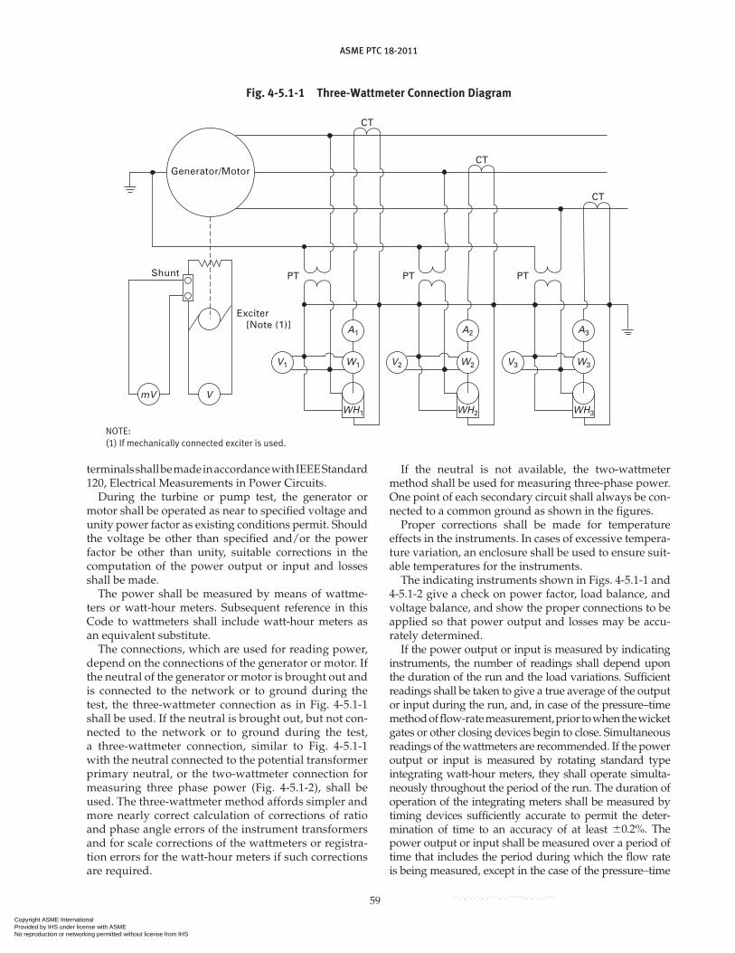
ASME PTC 18-2011

59

terminals shall be made in accordance with IEEE Standard 120, Electrical Measurements in Power Circuits.

During the turbine or pump test, the generator or motor shall be operated as near to specified voltage and unity power factor as existing conditions permit. Should the voltage be other than specified and/or the power factor be other than unity, suitable corrections in the computation of the power output or input and losses shall be made.

The power shall be measured by means of wattme-ters or watt-hour meters. Subsequent reference in this Code to wattmeters shall include watt-hour meters as an equivalent substitute.

The connections, which are used for reading power, depend on the connections of the generator or motor. If the neutral of the generator or motor is brought out and is connected to the network or to ground during the test, the three-wattmeter connection as in Fig. 4-5.1-1 shall be used. If the neutral is brought out, but not con-nected to the network or to ground during the test, a three-wattmeter connection, similar to Fig. 4-5.1-1 with the neutral connected to the potential transformer primary neutral, or the two-wattmeter connection for measuring three phase power (Fig. 4-5.1-2), shall be used. The three-wattmeter method affords simpler and more nearly correct calculation of corrections of ratio and phase angle errors of the instrument transformers and for scale corrections of the wattmeters or registra-tion errors for the watt-hour meters if such corrections are required.

If the neutral is not available, the two-wattmeter method shall be used for measuring three-phase power. One point of each secondary circuit shall always be con-nected to a common ground as shown in the figures.

Proper corrections shall be made for temperature effects in the instruments. In cases of excessive tempera-ture variation, an enclosure shall be used to ensure suit-able temperatures for the instruments.

The indicating instruments shown in Figs. 4-5.1-1 and 4-5.1-2 give a check on power factor, load balance, and voltage balance, and show the proper connections to be applied so that power output and losses may be accu-rately determined.

If the power output or input is measured by indicating instruments, the number of readings shall depend upon the duration of the run and the load variations. Sufficient readings shall be taken to give a true average of the output or input during the run, and, in case of the pressure–time method of flow-rate measurement, prior to when the wicket gates or other closing devices begin to close. Simultaneous readings of the wattmeters are recommended. If the power output or input is measured by rotating standard type integrating watt-hour meters, they shall operate simulta-neously throughout the period of the run. The duration of operation of the integrating meters shall be measured by timing devices sufficiently accurate to permit the deter-mination of time to an accuracy of at least 0.2%. The power output or input shall be measured over a period of time that includes the period during which the flow rate is being measured, except in the case of the pressure–time

Fig. 4-5.1-1 Three-Wattmeter Connection diagram

Exciter[Note (1)]

PT

WH1

PT PT

CT

CT

CT

Shunt

Generator/Motor

V1

VmV

WH2

V2 W2

A2

WH3

V3 W3

A3

W1

A1

NOTE:(1) If mechanically connected exciter is used.


--`,`,,`,`,``,,`,````,,`,````-`-`,,`,,`,`,,`---

ASME PTC 18-2011

60

method of flow rate measurement where the power output or input shall be measured immediately prior to when the wicket gates or other closing devices begin to close.

Instrument transformers used for the test shall be calibrated prior to installation or immediately prior to the test by comparison with standards acceptable to the parties to the test. When existing station (meter class) transformers are used, the burden of the transformer secondary circuits shall be measured with the test instru-mentation connected. If the burden of the transformers is exceeded, then station metering circuits may be tem-porarily disconnected for the duration of the test. The instrument transformers shall be tested to determine the ratio of transformation and the phase angle deviations for secondary burdens, which are equivalent to actual instrument burdens of the instruments to be used dur-ing the performance test. The correction data shall be available before the start of testing.

The burden of the current transformers and poten-tial transformers shall be checked after all power test equipment is connected. The voltage and current of the secondary loops of the transducers shall be measured as close to the secondary transformer terminals as pos-sible to ensure that all station and test equipment is on the load side of the measurements. Care should be taken to ensure that the burden measurement apparatus shall be placed on the source side of station instrumentation as shown on Fig. 4-5.1-3. As a word of caution, the second-ary loops of the potential transformers should never be shorted. Also, the secondary current transformers should

never be opened while the generator is running. The volt-age and current transformers volt-amp measurements shall be checked to ensure that the volt-amp rating is not exceeded. If measurements show that the secondary rat-ings are within 5% of their rated VA burden, then station equipment should be removed from the secondary loops before testing and the volt-amp burden of each secondary transformer loop shall be re-measured.

4-5.2 Windage and Friction

All generator or motor windage and friction losses shall be charged to the generator or motor and all tur-bine or pump friction losses shall be charged to the tur-bine or pump. During the generator or motor test, the turbine or pump should be uncoupled from the genera-tor or motor to permit determination of the generator or motor windage and friction.

If it is impractical to uncouple the turbine or pump during the generator or motor efficiency test, the approx-imate value of windage and friction of the machine may be calculated by the following formulas:

(a) Francis Turbine or Centrifugal Pump

P 5 Kf BD4n3

whereB 5 height of distributor, m (ft)D 5 outside diameter of runner, m (ft)Kf 5 empirical constant, the average value of which

is 3.8 3 1022 (1 3 1024)

Fig. 4-5.1-2 Two-Wattmeter Connection diagram

Exciter [Note (1)]

PT

WH1

PT

CT

CT

Shunt

Generator/Motor

V1

VmV

WH2

V2 W2

A2

W1

A1

NOTE:(1) If mechanically connected exciter is used.


--`,`,,`,`,``,,`,````,,`,````-`-`,,`,,`,`,,`---

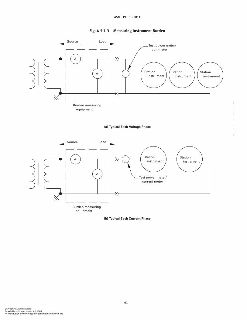
ASME PTC 18-2011

61

Fig. 4-5.1-3 measuring Instrument Burden

Source Load

Burden measuring equipment

A

V

Test power meter/ volt meter

Station instrument

Station instrument

Station instrument

(a) Typical Each Voltage Phase

Source Load

A

V

Station instrument

Station instrument

Test power meter/ current meter

Burden measuring equipment

(b) Typical Each Current Phase


--`,`,,`,`,``,,`,````,,`,````-`-`,,`,,`,`,,`---

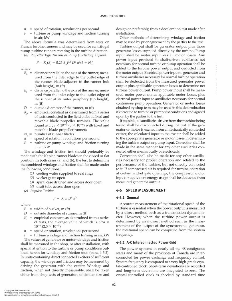
ASME PTC 18-2011

62

n 5 speed of rotation, revolutions per secondP 5 turbine or pump windage and friction turning

in air, kWThe above formula was determined from tests on

Francis turbine runners and may be used for centrifugal pump-turbine runners rotating in the turbine direction.

(b) Propeller Type Turbine or Pump (Including Kaplan)

P 5 Kp(Bt 1 0.25 Bh)0.5 D4 n3(5 1 Np)

whereBh 5 distance parallel to the axis of the runner, meas-

ured from the inlet edge to the outlet edge of the runner blade adjacent to the runner hub (hub height), m (ft)

Bt 5 distance parallel to the axis of the runner, meas-ured from the inlet edge to the outlet edge of the runner at its outer periphery (tip height), m (ft)

D 5 outside diameter of the runner, m (ft)Kp 5 empirical constant as determined from a series

of tests conducted in the field on both fixed and movable blade propeller turbines. The value found is 1.05 3 1023 (5 3 1026) with fixed and movable blade propeller runners

Np 5 number of runner bladesn 5 speed of rotation, revolutions per secondP 5 turbine or pump windage and friction turning

in air, kWThe windage and friction test should preferably be

made with the Kaplan runner blades in the closed or flat position. In both cases (a) and (b), the test to determine the combined windage and friction shall be made under the following conditions:

(1) cooling water supplied to seal rings(2) wicket gates open(3) spiral case drained and access door open(4) draft tube access door open

(c) Impulse Turbine

P 5 Ki B D4 n3

whereB 5 width of bucket, m (ft)D 5 outside diameter of runner, m (ft)Ki 5 empirical constant, as determined from a series

of tests, the average value of which is 8.74 3 1023 (2.3 3 1025)

n 5 speed or rotation, revolutions per secondP 5 turbine windage and friction turning in air, kWThe values of generator or motor windage and friction

shall be measured in the shop, or after installation, with special attention to the turbine or pump conditions out-lined herein for windage and friction tests (para. 4-5.2). In units containing direct connected exciters of sufficient capacity, the windage and friction may be measured by driving the generator with the exciter. Windage and friction, when not directly measurable, shall be taken either from shop tests of generators of similar size and

design or, preferably, from a deceleration test made after installation.

Other methods of determining windage and friction may be used by prior agreement by the parties to the test.

Turbine output shall be generator output plus those generator losses supplied directly by the turbine. Pump input shall be motor input less all motor losses. Any power input provided to shaft-driven auxiliaries not necessary for normal turbine or pump operation shall be added to the turbine power output and deducted from the motor output. Electrical power input to generator and turbine auxiliaries necessary for normal turbine operation shall be deducted from the measured generator power output plus applicable generator losses to determine net turbine power output. Pump power input shall be meas-ured motor power minus applicable motor losses, plus electrical power input to auxiliaries necessary for normal continuous pump operation. Generator or motor losses obtained by shop tests may be used in this determination if corrected to turbine or pump test conditions and agreed upon by the parties to the test.

If possible, all auxiliaries driven from the machine being tested shall be disconnected during the test. If the gen-erator or motor is excited from a mechanically connected exciter, the calculated input to the exciter shall be added to the appropriate generator or motor losses in determin-ing the turbine output or pump input. Correction shall be made in the same manner for any other auxiliaries con-nected either mechanically or electrically.

Correction shall also be made for any other auxilia-ries necessary for proper operation and related to the performance of the turbine, but not directly connected to it. If compressed air is required for turbine operation at certain wicket gate openings, the compressor motor input or equivalent energy usage shall be deducted from measured generator output.

4-6 SPEEd mEASUREmENT

4-6.1 General

Accurate measurement of the rotational speed of the turbine is essential when the power output is measured by a direct method such as a transmission dynamom-eter. However, when the turbine power output is determined by an indirect method such as the meas-urement of the output of the synchronous generator, the rotational speed can be computed from the system frequency.

4-6.2 A-C Interconnected Power Grid

The power systems in nearly all the 48 contiguous states and many of the provinces of Canada are inter-connected for power exchange and frequency control. System frequency is compared to a very high-grade crys-tal-controlled clock. Short-term deviations are recorded and long-term deviations are integrated to zero. The crystal-controlled clock is checked by standard time


--`,`,,`,`,``,,`,````,,`,````-`-`,,`,,`,`,,`---

ASME PTC 18-2011

63

signals transmitted by the United States National Institute of Standards and Technology radio station WWV located at Fort Collins, CO.

For a turbine or pump test with a synchronous gen-erator or motor connected to an alternating current interconnected grid, the speed is not expected to vary from true interval by more than 0.02% under normal operating conditions. For a Code test, the actual system frequency must be measured somewhere in the power system and its value recorded.

4-6.3 Isolated Alternating Current Systems or Short-Term measurements

Electronic timers and counters that are available can be used in two ways. A crystal-controlled time base accurately measures pulses for a period of 1 s to 10 s. During a preset period, the counter integrates the number of cycles or pulses. Alternatively, using the same equipment, time for one cycle is measured. A 1-MHz timing crystal will read 16.667 ms for one cycle. The "hold" time can be set for one second to allow a reading, and then another cycle is sampled automatically.

4-6.4 Induction Generators of motors or direct Current System

The first choice in this case is a mechanically driven revolution counter using the same electronic equip-

ment as above. A projection on the shaft provides an electrical pulse either by contactor or electromagnetic pickup.

The electronic devices mentioned above are provided with an independent crystal oscillator as a time base. The frequency of this crystal shall be checked in the lab-oratory before the test.

Pulse generating wheels must be solidly connected to the unit shaft. Tachometer generators shall be driven by a mechanical connection such as a flexible shaft. Friction or belt drives shall not be used.

4-7 TImE mEASUREmENT

The most accurate measurement and portable time base available at present is a crystal-controlled oscilla-tor. All manufacturers of crystal oscillators offer crystal oscillators that are temperature-compensated. Typically, temperature-compensation ranges [08C to 508C] encom-pass what is normally found in ambient temperatures. Uncertainties vary from 1 ppm for a crystal that is temperature-compensated, to 300 ppm when not tem-perature compensated. Crystal-controlled oscillators shall be checked for stability and drift. Oscillators used in field-testing applications should be temperature-compensated. They shall be operated according to the manufacturer’s instructions.


--`,`,,`,`,``,,`,````,,`,````-`-`,,`,,`,`,,`---

ASME PTC 18-2011

64

5-1 mEASUREd VAlUES: dATA REdUCTION

Following each test, when all test logs and records have been completed and assembled, they should be examined critically to determine whether or not the limits of per-missible deviations from specified operating conditions have exceeded those prescribed by the individual test code. Adjustments of any kind should be agreed upon and explained in the test report. If adjustments cannot be agreed upon, the test run(s) may have to be repeated. Inconsistencies in the test record or test result may require tests to be repeated in whole or in part in order to attain test objectives. Corrections resulting from deviations of any of the test operating conditions from those specified are applied when computing test results.

The averages of the readings or recordings with appro-priate calibrations and/or corrections for each run shall be used for the computation of results. Any reading sus-pected of being in error shall be tested by the criteria for outliers in Nonmandatory Appendix C. Preliminary computations (subsection 3-3) made during the course of the test, together with plots of important measured quantities versus wicket-gate servomotor stroke, are useful for indicating errors, omissions, and irregulari-ties, and shall appear in the final report as a reference.

Before disconnecting any instruments, all test logs and records shall be completed and assembled, and then critically examined to detect and correct or elimi-nate irregularities. It should be determined also at that time whether or not the limits of permissible deviations (para. 3-5.2) from specified operating conditions, and/or the limits of permissible fluctuations (para. 3-5.3), have been exceeded.

Prompt examination of readings may indicate the need for inspection and adjustment of the machine or of test instrumentation, thereby minimizing the number of runs that may have to be voided and repeated.

The averages of all readings shall be corrected using the average of the pretest and post-test calibration curves for each instrument.

5-2 CONVERSION OF TEST RESUlTS TO SPECIFIEd CONdITIONS

5-2.1 Turbine mode

When the readings indicate that test conditions have complied with the requirements of paras. 3-5.2 and 3-5.3(a), the measured flow rate (QT) and turbine power

output (PT) at head (HT) shall be converted to the values for specified head (Hspec) by

Q H QH

HTT

at specspec

0.5

�

P H PH

HTT

at specspec

1.5

�

When the test conditions have complied with the above provisions, the turbine efficiency, which requires no correction, is (SI Units)

��

� � �turbine power output ( )

water power ( )

1 000 1

spec

P

P

P

gQHW

000P

gQ HT

T T�

(U.S. Customary Units)

��

�550

spec

P

gQH

Values of and g are given in Tables 2-3-4 and 2-3-2, respectively.

When the test conditions have complied with the provisions of paras. 3-5.2 and 3-5.3(b), but not with para. 3-5.3(a), the values of Q for Hspec and P for Hspec as calculated above shall be corrected to Q’ and P’, respec-tively, by multiplicative factors derived from known characteristic curves of a previously tested homolo-gous turbine, by the following steps:

Step 1: For each run, the following is calculated:

kn D

gHuTT

T

5p

560(2 )

speed coefficient0.5

q QD HT T

T

5 51

unit flow rate2 0.5

p PD HT T

T

5 51

unit power output2 1.5

where D equals runner diameter, and “unit” means rationalized to 1 m diameter, 1 m head (1 ft diameter, 1 ft head).

Step 2: Using the above referenced test curves determine

Section 5Computation of Results


--`,`,,`,`,``,,`,````,,`,````-`-`,,`,,`,`,,`---

ASME PTC 18-2011

65

p’ 5 unit power at specified head and speed coeffi-cient (ku-spec) for the gate opening that produces qT at kuT

q’ 5 unit flow rate at specified head and speed coef-ficient (ku-spec) for the gate opening that pro-duces qT at kuT

where

kn D

gHu-specspec

spec

�π

6 2 0 50 ( ) .

Step 3: Calculate flow rate and power at specified head by

′′

Q T5 Qq

q

H

HT

spec

T

0 5.

′′

P T5 Pp

p

H

HT

spec

T

1 5.

5-2.1.1 Efficiency. The corrected values, Q’ and P’, at Hspec shall be used to calculate the efficiency at each test run.(SI Units)

′′

′

5

1 000P

g HspecQ


��

' �550

g spec

′′P

Q H

A curve of efficiency as a function of power shall be plotted.

5-2.2 Pump mode

Assuming that the measured values indicate that test conditions have complied with the requirements of paras. 3-5.2 and 3-5.3(a), the calculated test results shall be converted to the specified speed (nspec) by using the following equations:

Q at n Qn

nTT

specspec

�

H at n Hn

nTT

specspec

�

2

NPSH at n NPSHn

nTT

specspec

�

2

P at n Pn

nTT

specspec

�3

Where the test conditions have complied with the provisions of para. 3-5.3(a),the machine efficiency (), which requires no correction for these conversions, is given by

(SI Units)

5gQ

P

H

1 000


��

=gQH

P550

Where the test conditions have complied with the provisions of para. 3-5.3(b) but not with those of para. 3-5.3(a), the values of Q at nspec; H at nspec; and P at nspec shall be adjusted by the addition (or subtraction) of incre-mental values Q, H, and P, respectively, derived by reference to characteristic curve of previously tested homologous machine.

5-2.2.1 Efficiency. The machine efficiency, ’, using the corrected values of

Q’ 5 Q 1 Q at nspec H’ 5 H 1 H at nspec P’ 5 P 1 P at nspecis given by

(SI Units)

′′ ′

′

5

g

P

Q H

1 000


′′ ′

′

5

gQ H

P550

Values of and g are given in Tables 2-3-4 and 2-3-2, respectively.

A curve of efficiency as a function of flow rate shall be plotted.

5-3 EVAlUATION OF UNCERTAINTy

Regardless of the excellence of the test, there will always be an uncertainty in the result. The uncertainty of the final results and all intermediate results shall be estimated using the general procedures described in Nonmandatory Appendix B, which is a summary of the more complete treatment in the current version of PTC 19.1.

5-4 COmPARISON WITH GUARANTEES

Turbines are usually guaranteed for power output and efficiency at one or more specified net heads. Efficiency may be guaranteed at one or more specified power out-puts or wicket gate or needle openings. All guarantees are at the specified synchronous speed unless otherwise stated.

Pumps are usually guaranteed for flow rate and effi-ciency at one or more specified heads.


--`,`,,`,`,``,,`,````,,`,````-`-`,,`,,`,`,,`---

ASME PTC 18-2011

66

Efficiency may be guaranteed at one or more flow rates. All guarantees are at specified speed unless stated otherwise.

When the head varies during the test, the values of effi-ciency and power output or flow for several heads may be determined. In such instances, a mean curve of guaranteed efficiency for comparison with the test curve of efficiencies at mean head can be determined by interpolation.

Test results shall be reported as actual com puted val-ues, corrected for instrument calibrations and converted to specified conditions. A statement shall be included in the test report that results are estimated to have a plus or minus percentage uncertainty, as determined by evaluation of uncertainties described in Nonmandatory Appendix B.


--`,`,,`,`,``,,`,````,,`,````-`-`,,`,,`,`,,`---

ASME PTC 18-2011

67

6-1 RESPONSIBIlITy OF CHIEF OF TEST

The chief of test shall be responsible for preparation of the final report and shall sign the report.

6-2 PARTIES TO THE TEST

The parties to the test shall receive copies of the draft and final report.

6-3 ACCEPTANCE TESTS

For acceptance tests, the report shall include(a) a brief summary of the purpose of the tests, the

principal results, and conclusions.(b) description of special conditions or pretest

agreements.(c) identification of the parties to the test and a list of

the key personnel taking part in the test, including their organizational affiliations.

(d) a summary of the specified operating conditions and guarantees.

(e) descriptions, drawings, and/or photographs of the machine under test, the plant layout, inlet condi-tions, and outlet conditions, including any unusual fea-tures that may influence test results.

(f) the names of manufacturers and nameplate data listing power, flow rate, speed, and head.

(g) description of the inspected water passages, pres-sure taps, and underwater components.

(h) description of the test equipment and test proce-dures, including the arrangement of the equipment and list of instruments. Instrumentation descriptions should include manufacturer, key specifications, manufactur-er’s stated accuracy, identifying number or tag, owner, length and type of electrical leads (where relevant), cali-bration curves, and certificates of calibration.

(i) test date.(j) log of test events.

(k) tabulations or summaries of all measurements and uncorrected readings.

(l) methods of calculation for all quantities computed from the raw data.

(m) reference information such as generator efficiency curve.

(n) copies of instrumentation calibration documentation.(o) corrections for deviations from specified

conditions.(p) statement regarding cavitation factor observed

during the tests.(q) analysis of the uncertainty of the test results.(r) summary of results.(s) tabular and graphical presentation of the final test

results.(1) For turbines, the graphical presentation

should include(a) efficiency versus power output(b) flow rate versus power output(c) power output versus wicket gate opening

or needle position and blade angle, where applicable(d) flow rate versus wicket gate opening or

needle position and blade angle, where applicable(2) For pumps, the graphical presentation should

include(a) head versus flow rate(b) flow rate versus power input(c) efficiency versus flow rate(d) efficiency versus wicket gate opening

(t) appendices as required to describe details of dimensions of water passages, additional drawings and illustrations as needed for clarification, and any other supporting documentation that may be required to make the report a complete, self-contained document of the entire test.

(u) documentation of any unresolved disagreements between the parties to the test.

Section 6Final Report


--`,`,,`,`,``,,`,````,,`,````-`-`,,`,,`,`,,`---

68

INTENTIONAlly lEFT BlANK


--`,`,,`,`,``,,`,````,,`,````-`-`,,`,,`,`,,`---

ASME PTC 18-2011

69

NONmANdATORy APPENdIX ATyPICAl VAlUES OF UNCERTAINTy

A-1 GENERAl

Uncertainties in this Code are specified at the 95% confidence interval as described in Nonmandatory Appendix B. The following paragraphs present typical uncertainties (including both systematic and random errors) that may be attainable with calibrated instru-mentation and normal test conditions.

The values listed below for specific measurements are for general guidance only and should not be used without supporting calculations and verifications. Systematic and random uncertainties should be calcu-lated in accordance with Nonmandatory Appendix B and the current version of PTC 19.1. This general list is not comprehensive, and all uncertainties associated with each test measurement should be identified and separately addressed.

A-2 FlOW RATE UNCERTAINTy, UQ

(a) Current meter method(1) conduits from 1.2 m to 1.5 m (4 ft to 5 ft) diam-

eter, 1.2%(2) conduits of more than 1.5 m (5 ft) diameter,

1.0%(b) Pressure–time method, 1.0%(c) Ultrasonic method (two crossing planes, four

paths each), 1.0%(d) Dye dilution method, 1.5%

A-3 HEAd UNCERTAINTy, UH

(a) Measurement of free water level difference, h (1) point gage, hook gage, or float gate

(a) (1/h)% (SI Units)(b) (3.2/h)% (U.S. Customary Units)

(2) plate gage, fixed(a) (5/h)% (SI Units)(b) (16.4/h) % (U.S. Customary Units)

(b) Pressure uncertainty (1) deadweight gage, 0.1%

(2) height of mercury, h’(a) (0.1/h)% (SI Units)(b) (0.32/h)% (U.S. Customary Units)

(c) Spring pressure gage, 0.5%(d) Transducers, (0.1 to 0.5)%

A-4 POWER UNCERTAINTy, UP

(a) By measurement at the terminals of(1) DC generators, 1.0%(2) AC generators, 0.5%

(b) Depending upon the method employed for the determination of generator losses, and in cases where shunts are used for large direct currents, Up may be greater than the above values. For example, the uncer-tainty in power at a test point can be calculated as follows:

(1) watt/watthour meter uncertainty: 0.25%(2) potential transformer uncertainty: 0.5%(3) current transformer uncertainty: 0.5%(4) timer uncertainty: 0.0001%(5) uncertainty in generator efficiency: 0.1%

(c) The calculated uncertainties are then computed as described in Nonmandatory Appendix B from the root- sum-square of the above uncertainties as follows:

UP 5 1 1 1 1(0.25 0.5 0.5 0.0001 0.1 )2 2 2 2 2 0.5

UP 5 0.76%

At other measuring points, the overall uncertainty would be different. With the use of accurate modern elec-tronic instrumentation, it may be significantly smaller.

A-5 SPEEd UNCERTAINTy

Electric counter and other precision speed measuring devices 5 0.1%.


--`,`,,`,`,``,,`,````,,`,````-`-`,,`,,`,`,,`---

ASME PTC 18-2011

70

B-1 BASIS FOR UNCERTAINTy CAlCUlATION

Regardless of the care taken in their design and imple-mentation, all tests will yield measurements and results that are different from the true values that would have been determined with perfect measurements. Thus, the true or exact result is uncertain. The objective of the uncertainty analysis is to rationally quantify the uncer-tainty in the test results (e.g., machine efficiency).

This Nonmandatory Appendix presents an approach to uncertainty analysis that is commonly used in the hydroelectric industry. It differs from the more rigorous approach presented in PTC 19.1, Test Uncertainty, in the handling of Student’s t statistic and the associated deter-mination of the number of degrees of freedom.

Because hydroturbine efficiency measurements often have sample sizes on the order of 5 measurements (e.g., determination of peak efficiency as a contractual guarantee), the assumption that t 5 2 (large degrees of freedom) is not always justified. In these cases, the approach presented here differs from that of PTC 19.1 in that the t statistic is applied to each elemental uncer-tainty with degrees of freedom determined from the individual sample sizes, instead of applying a single value of t with degrees of freedom determined by the Welch–Satterthwaite formula to the combined elemental uncertainties.

In the case of large sample sizes, the two approaches yield identical results. In the case of small sample sizes, the approach presented here will generally yield slightly larger uncertainties.

Uncertainties for this Code are computed at the 95% confidence level. This means that for any measurement or computed result, the true result is expected to be within the uncertainty value of the measured result 95% of the time. Conversely, the true result will not be within the uncertainty value of the measured result 5% of the time.

The summary presented here applies only to the case in which the various uncertainties can be considered independent of one another. The latest version of PTC 19.1 should be consulted if there is any question as to the applicability of this assumption.

B-2 SUmmARy OF mETHOdOlOGy

The methodology presented here uses turbine mode efficiency as an example. This basic methodology

applies to any part of the uncertainty analysis, e.g., the detailed determination of the uncertainty in the head measurement.

The basic steps in determining the uncertainty of any parameter are as follows:

(a) Develop the equation or equations that define the desired result in terms of the measurements (or param-eters) upon which the results depend.

(b) Determine how sensitive the desired result is to changes in the parameters from which it is computed.

(c) Determine the uncertainty in these parameters.(d) Use the sensitivity determined above to quantify

the effect on the result of uncertainty in each parameter upon which it depends.

(e) Combine these individual uncertainty effects to determine the overall uncertainty of the final result.

B-3 GENERAl APPROACH ANd TURBINE EFFICIENCy EXAmPlE

The general approach for uncertainty analysis is pre-sented here, using turbine efficiency as an example. The equation that defines turbine efficiency is

T gQH5

PT

The uncertainty in the measured efficiency will there-fore be a function of the uncertainty in the measurements of turbine power, PT; flow, Q; net head, H; water den-sity, ; and gravity, g. Each of these measurements will depend, in general, upon the results of measurements of several other parameters. For instance, net head will depend on both the static and velocity heads at the inlet and the discharge. Consequently, it will depend on the measurements of flow rate, conduit area, inlet pressure, discharge pressure, etc.

For any individual parameter, P, the uncertainty in the measurement is determined by a combination of systematic uncertainties that are generally due to uncer-tainty in instrumentation calibrations, geometric meas-urements, etc., and random uncertainties that generally arise from variations in the quantity being measured or noise in the measurement system.

The systematic uncertainty, B, is determined from analysis of calibration equipment, calibration history, measuring equipment, manufacturer’s specifications, published guidelines, etc. The random uncertainty, S, is generally determined from the statistics of the

NONmANdATORy APPENdIX BUNCERTAINTy ANAlySIS


--`,`,,`,`,``,,`,````,,`,````-`-`,,`,,`,`,,`---

ASME PTC 18-2011

71

measurement record. Under the assumptions stated earlier in this Appendix, a measure of the random uncertainty is the standard deviation, SP , about the mean of N measurements of an individual parameter, P, at a particular test condition. The standard devia-tion is defined as

SN

P PP ii

N

52

25

1

12

1

12

( )∑

wherePi 5 individual measured value of parameter P

P 5 the average of the measured values of parameter PThe random uncertainty in actual value of the mean

SP is given by

S t S NP P5

where t 5 Student’s t-statistic for adjusting to the 95%

confidence interval (see Table B-3-1)This equation for SP

shows that the random uncer-tainty can be reduced by taking more measurements, N, with the caveat that the measurements be spaced far enough apart that there is no correlation of the random component between the individual measurements.

The overall uncertainty, UP, in the measured value of a parameter, P, is then given by the root-sum-square (RSS) equation

U B tSP P P5 12 2( )

When a result is determined from several individual parameters, the individual (elemental) systematic and random uncertainties are combined by the RSS method.

B B BP P P PK5 1 1 112

22 2

B

and

S tS tS tSP P P PK5 1 1 1( ) ( ) ( )12

22 2

where BPI and tSPI are the elemental systematic and ran-dom uncertainties, respectively.

The final result of an uncertainty calculation does not depend on the order in which the combining of the elemental uncertainties is performed. Under the RSS method, the same result is obtained if all system-atic and random uncertainties are computed separately, then combined; if the systematic and random uncer-tainties for an individual measurement are computed

Table B-3-1 Two-Tailed Student's t Table for the 95% Confidence level

Degrees of Freedom 5 n – 1 t

Degrees of Freedom 5 n – 1 t

1 12.706 16 2.120

2 4.303 17 2.110

3 3.182 18 2.101

4 2.776 19 2.093

5 2.571 20 2.086

6 2.447 21 2.080

7 2.365 22 2.074

8 2.306 23 2.069

9 2.262 24 2.064

10 2.228 25 2.060

11 2.201 26 2.056

12 2.179 27 2.052

13 2.160 28 2.048

14 2.145 29 2.045

15 2.131 30 2.042

GENERAL NOTE: Student’s t may be computed from the following empiri-cal equation for other values of :

t 5 1 11 962 36 3 2 5 2

2 3 84.. . .

. +


--`,`,,`,`,``,,`,````,,`,````-`-`,,`,,`,`,,`---

ASME PTC 18-2011

72

and combined, and the measurement uncertainties are combined over all measurements; or if all elemental sys-tematic and random uncertainties are combined in one step. However, it is often useful to determine the overall systematic and random uncertainties separately, as this may give insight as to the most likely areas for improve-ment in test uncertainty.

The relative sensitivity of a result, R, due to changes in a particular parameter, P, is given by using a Taylor series approximation to define a sensitivity coefficient for the parameter, TP

TR

PP 5∂∂

The uncertainty in the result, R, due to the uncer-tainty in the parameter, P, is then given by

R 5 TP P

Returning to turbine efficiency as an example, the sensitivity coefficients for efficiency, , can be computed from the efficiency equation

TP gHQP

T

5 5

1

TP

gH QHT

5 52

H 2

Tg

P

g HQgT

5 52

2

TQ

P

gHQQT

� ��

� � 2

TP

gHQT

�

��

� �� 2

The overall uncertainty in the efficiency, E, is then given by

E T P T Q T H

T T g

p T Q H

g

� � � �

� �

= ( ) ( ) ( )

( ) ( )

� � �

� �

� �

� �

2 2 2

2 2 1 2

� �/

The relative uncertainty in efficiency, U, can be deter-mined from the preceding equations to be

UE P

P

Q

Q

H

HT

T

5 5

+

+

+

+

2 2 2 2ρρ

gg

g

2 1 2/

The determination of the density of water is usu-ally based on temperature measurement of the water. With an ordinary thermometer, this parameter is easily measured within 28C uncertainty. At 208C, this uncer-tainty leads to a relative uncertainty in the density of only about 0.04%. Thus, the uncertainty in density may be neglected. A similar line of reasoning applies to the determination of g.

B-4 COmBINING UNCERTAINTIES

Several other useful specific forms derived from the Taylor series method for propagation of uncertainties are given below.

B-4.1 Average of Two or more Parameters

If a result is computed as an average of two parameters

R x y5 112 ( )

then the uncertainty in the result is given by

U U UR x y5 112

2 21

2( )Averages for more than two parameters can be com-

puted in similar fashion. For instance, if three parameters are averaged to determine a result, then the uncertainty in the result is given by

U U U UR 5 1 113 1

222

32

12( )

This combining of uncertainties for a result computed from an average is referred to as RSS averaging of the uncertainties.

NOTE: If the elemental uncertainties, Ui, are equal (for instance, in the measurement of flow rate in three intake bays of a Kaplan unit), the RSS average of three uncertainties is given by

UU

R 53

where U1 5 U2 5 U3 5 U. A similar result is obtained for any number of averaged parameters.

B-4.2 Sum or difference of Two or more Parameters

If a result is computed as the sum or difference of two parameters

R 5x y

then the uncertainty in the result is given by

U U UR x y5 12 21

2( )Sum or differences of more than two parameters can

be computed in similar fashion. For instance, if three parameters are summed to determine a result, then the uncertainty in the result is given by

UR U U U5 1 112

22

32

12( )

NOTE: If the elemental uncertainties, Ui, are equal, the RSS sum of three uncertainties is given by

U UR 5 3

where U1 5 U2 5 U3 5 U. A similar result is obtained for any number of summed parameters.


--`,`,,`,`,``,,`,````,,`,````-`-`,,`,,`,`,,`---

ASME PTC 18-2011

73

B-5 APPlICATION OVER A RANGE OF OPERATING CONdITIONS

Measurements (e.g., power output) or determinations of results (e.g., turbine efficiency) of parameters over a range of operating conditions may be expected to fol-low a smooth curve. For instance, turbine efficiency (the dependent parameter) may be expected to be a smooth function of the power output (the independent param-eter) for a given head. However, test measurements or results will deviate from a smooth curve plotted over a range of operating conditions, reflecting random (repeat-ability) errors in the underlying measurements. The deviation of these computed results from the smooth curve can be used to determine the uncertainty of a result over a range of operating conditions. In practice, the smooth curve fits are often made using polynomials of up to the fifth order, although other functions may be employed. The use of a least-squares curve fit to relate the two parameters is the most common method of fit-ting the smooth curve.

The standard deviation of the sample mean in this case is the standard deviation of the difference of the inde-pendent measured parameter (e.g., turbine efficiency) from the curve fit to that parameter as a function of the independent parameter. For instance, suppose turbine efficiency, , is plotted as a function a power output, P, and a fifth-order polynomial relating these two param-eters is determined by a least-squares technique, result-ing in the following relationship:

�� c c P c P c P c P c Po 1 22

33

44

55

where the c0 through c5 are the polynomial coefficients. The standard deviation of the difference between the test efficiencies and the curve fit is then given by

SN M i

i

N

� � ��

� �

1

12

1

1 2

( )/

∑

�

wherei 5 individual efficiencies�� 5 curve fit of the efficiency as a function of powerN 5 number of measurementsM 5 number of coefficients to be determined (for the

polynomial coefficients in the example above, M 5 6).The standard deviation of the sample mean for the

turbine efficiency over the range of power outputs is then given by

S S N 5

It should be noted that the random error determined from a curve fit will depend not only upon the scatter in the measurements, but also upon the appropriateness of the curve used for the curve fit. For instance, if turbine efficiency is considered as a function of power output, a second-order polynomial generally will not follow the true curve very well. This will lead to a relatively high estimate of uncertainty. The use of a higher-order curve may reduce this uncertainty while retaining the smoothness and reasonableness of the curve. However, care must be used, and the fit curve should be plot-ted and investigated for reasonableness. For polyno-mial curve fits, for instance, the number of data points should be at least 1.5 to 2 times the order of the curve fit. Fitting a fifth-order curve to six data points may result in a wildly oscillating curve. Experience has also shown that polynomial curve fits greater than fifth order often yield unsuitable curves. Such unreasonableness can be detected by simply plotting and inspecting the derived curve fit.


--`,`,,`,`,``,,`,````,,`,````-`-`,,`,,`,`,,`---

ASME PTC 18-2011

74

All measurement systems may produce spurious data points, also known as outliers, strays, mavericks, rogues, or wild points. These points may be caused by tempo-rary or intermittent malfunctions of the measurement system. Data points of this type shall not be included as part of the uncertainty of the measurement. Such points are considered to be meaningless as steady-state test data, and shall be discarded.

The modified Thompson technique is recommended for testing possible outliers. The following is a sum-mary of the technique. A more complete discussion with example is given in PTC 19.1-2005.

Let yi be the value of the observation, y, that is most remote from Y� , the arithmetic mean value of all observa-tions in the set, and S be the estimated standard devia-tion of all observations in the set. Then if the value, without regard to sign, of

d y Yi� � �

is greater than the product S, the value yi is rejected as an outlier. The value of is obtained from Table C-1.

After rejecting an outlier, Y� and S are recalculated for the remaining observations. Successive applications of this procedure may be made to test other possible out-liers, but the usefulness of the testing procedure dimin-ishes after each rejection.

All sets of readings should be examined for outliers before computations are made. All significant quanti-ties, such as Q, H, P, and n, should be tested for outliers. The test should also be applied to curves fit to test data over a range of operating conditions.

NONmANdATORy APPENdIX COUTlIERS

Table C-1 modified Thomspon Values (at the 5% Significance level)

Sample Size, N Sample Size, N

3 1.150 22 1.893

4 1.393 23 1.896

5 1.572 24 1.899

6 1.656 25 1.902

7 1.711 26 1.904

8 1.749 27 1.906

9 1.777 28 1.908

10 1.798 29 1.910

11 1.815 30 1.911

12 1.829 31 1.913

13 1.840 32 1.914

14 1.849 33 1.916

15 1.858 34 1.917

16 1.865 35 1.919

17 1.871 36 1.920

18 1.876 37 1.921

19 1.881 38 1.922

20 1.885 39 1.923

21 1.889 40 1.924


--`,`,,`,`,``,,`,````,,`,````-`-`,,`,,`,`,,`---

ASME PTC 18-2011

75

d-1 dEFINITIONS

An index test is a method for determining the relative effi-ciency of a machine based on relative flow measurement. An index value is an arbitrarily scaled measure. Relative values are derived from the index values by expressing them as a proportion of the index value at a stipulated con-dition. Power and head are measured by any of the meth-ods in this Code. Flow rate is measured as an index value by measuring a parameter that is a function of flow, such as differential pressure across a tapered section of penstock or Winter–Kennedy taps. Relative efficiency is expressed as a proportion of peak index efficiency.

d-2 APPlICATION

An index test may be used alone or as part of a per-formance test for any of the following purposes:

(a) to determine relative flow and efficiency in con-junction with turbine power output or pump power input. Such performance characteristics may be com-pared with the performance predicted from tests on a homologous model.

(b) to determine the overall operating point or points that define the most efficient operation or to extend information on performance over a wider range of net head, flow rate, or power than covered by performance tests.

(c) to determine the relationship between runner blade angle and wicket-gate opening for most efficient operation of adjustable blade turbines, and for the pur-pose of calibrating the blade control cam.

(d) to determine the optimum relative efficiency wicket-gate opening at various heads for pump operation.

(e) to assess the change in efficiency due to cavitation resulting from a change in lower pool level and/or net head.

(f) to monitor flow-rate data during the performance test.

(g) to obtain calibration data for permanent pow-erhouse flow-measuring instruments by assuming an absolute value of machine efficiency at some operating point.

(h) to assess the change in performance of the machine resulting from wear, repair, or modification.

When an index test is used to supplement results of a performance test, measurements of flow rate made for

the performance test are used to calibrate the index of flow. The index test results may then be expressed in terms of efficiency rather than relative efficiency. In this case, the results should include a statement concerning the accuracy and confidence limits that apply to the cali-bration of flow-rate measurement.

For some applications, the index test may be used to obtain the combined relative efficiency of the turbine-generator unit or pump-motor unit.

d-3 RElATIVE FlOW RATE

d-3.1 General

An index test does not require any absolute measure-ment of flow rate. Examples of relative flow-rate meas-urement methods include the following:

(a) measurement of the pressure differences existing between suitably located taps on the turbine spiral or semi-spiral case (see para. D-3.2). This is the Winter–Kennedy method, described in ASCE paper, “Improved Type of Flow Meter for Hydraulic Turbines,” by I. A. Winter (April 1933). This method is not suitable for relative flow meas-urement for pump operation.

(b) measurement of the pressure difference across a converging taper section of the penstock using the prin-ciple of a Venturi (see para. D-3.3).

(c) measurement of the difference between the eleva-tion of water in the inlet pool and the inlet section of the machine (see para. D-3.4).

(d) measurement of differential pressure between two piezometers located on a conduit elbow (see para. D-3.5).

(e) measurement of differential pressure between suitably located taps on a bulb or tubular turbine (see para. D-3.6).

Differential pressure measurements should not be made at turbine discharge sections, low-pressure pump intake sections, or other sections where pressure varia-tions are high in comparison with the total differential pressure, since the accuracy of the relative flow rate measurement will be significantly diminished.

Flow rate is taken as proportional to the nth exponent of the differential-pressure head [i.e., Qrel 5 k(h)n]. An approximate value of exponent n is 0.5. However, the value of the exponent may vary with the type of inlet case or conduit where relative flow is being measured, the location of the taps, and the flow rate. When an index test is part of the performance test, the value of n can be

NONmANdATORy APPENdIX dRElATIVE FlOW mEASUREmENT–INdEX TEST


--`,`,,`,`,``,,`,````,,`,````-`-`,,`,,`,`,,`---

ASME PTC 18-2011

76

determined from measurements of flow rate made for the performance test.

Measurement of the needle stroke may be used on impulse turbines to determine an index of flow rate pro-vided the needle stroke-versus-discharge characteristic shape has been checked by tests on a homologous model of the turbine needle valve. Care shall be taken to ensure that the needle, nozzle, and support vanes are clean and in good order during the test.

d-3.2 Relative Flow Rate measurement by the Winter–Kennedy method

The Winter–Kennedy method requires two pressure taps usually located in the same radial section of the spi-ral or semispiral case. See Figs. D-3.2-1 and D-3.2-2. One tap is located at the outer radius of the spiral or semispiral case, often on the horizontal (turbine distributor) center-line. The other tap is located at an inner radius outside the stay ring. Sometimes more than one tap is provided at the inner radius. The taps shall not be near rough-weld joints or abrupt changes in spiral or semispiral case section. The inner taps shall lie on a flow line between stay vanes.

d-3.3 Relative Flow measurement by the Converging Taper method

Two pressure taps shall be located at different size cross-sections of the conduit. The most stable pressure

difference will be obtained if both taps are in the con-verging section of the conduit. The differential pressure thus obtained is not the maximum possible; therefore, it may be preferable to locate one tap a short distance upstream of the convergence and the second not less than half a diameter downstream of the convergence.

d-3.4 Relative Flow Rate by the Friction Head loss and Velocity Head method

The difference between the elevation of the water in the inlet pool (upper pool for turbine and lower pool for pump) and the pressure head near the entrance to the machine may be used to measure the relative flow rate. The differential reading consists of the friction head and other head losses between the inlet pool and the sec-tion at the point of measurement near the entrance to the machine, plus the velocity head at this section.

Attention should be given to the trash rack to ensure that the head loss through the trash rack is not affected by an accumulation of trash during the test.

For pumps, the section near the entrance to the machine shall be selected so that the proximity to the runner is not causing rotational flow, which can influence the pressure head reading. At installations with long high-pressure conduit, relative flow for pumps can be measured on the discharge conduit, provided that the measuring sec-tion on the high-pressure side of the pump is selected so that rotational flow from the pump discharge is not

Fig. d-3.2-1 location of Winter–Kennedy Pressure Taps in Spiral Case

Section A–A

1

1

2

2

Outer (high pressure) tap

Inner (low pressure) taps, select one

3

3

A

A

15 to 90 deg


--`,`,,`,`,``,,`,````,,`,````-`-`,,`,,`,`,,`---

ASME PTC 18-2011

77

influencing the pressure head reading. Often the net head taps on the pump inlet conduit (draft tube on a pump-turbine) versus tap(s) near the runner can be used.

If more than one machine is connected to the same conduit, the machine(s) other than the one under test shall be shut down, and the leakage through the wicket gates or shutoff valves of the other turbine(s) shall be measured, calculated, or estimated.

d-3.5 Relative Flow measurement as a differential Across an Elbow

The differential-pressure readings between two pres-sure taps located on a penstock elbow may be used to determine relative flow rate.

d-3.6 Relative Flow measurement Using Suitably located Taps on a Bulb or Tubular Turbine

Relative flow rate may be determined by measur-ing the differential pressure between a single high-

pressure tap located at the stagnation point at the front of the bulb or the front of the access shaft to the bulb, and two low-pressure taps mounted on the converging section of turbine casing upstream of the wicket gates. The pressure taps must be located a sufficient distance upstream of the wicket gates so that the flow patterns at the pressure taps are not influenced by the wicket gate position.

d-3.7 Pressure Taps and Piping

The pressure taps shall comply with the dimensional requirements of para. 4-3.14. Since the differential heads to be measured may be small, special attention shall be given to removing surface irregularities.

When relative flow measurement is made over a long period of time, or if separate index tests are made at dif-ferent times to assess the change in efficiency of a machine from wear, repair, or modification, it is necessary for the condition of the pressure taps and surrounding area to

Fig. d-3.2-2 location of Winter–Kennedy Pressure Taps in Semi-Spiral Case

Outer (high pressure) tap

Inner (low pressure) tap2

1

1

2

A

A

Section A–A

15 to 90 deg


--`,`,,`,`,``,,`,````,,`,````-`-`,,`,,`,`,,`---

ASME PTC 18-2011

78

remain unchanged for the relative flow rate and/or rela-tive efficiency to be comparable.

When the pressure taps are calibrated using a Code-approved method of measuring flow rate (subsection D-4), it is essential that the taps remain in their as-cali-brated condition to give accurate results over time. This includes keeping the trash racks clean, as the pressure profile at the pressure-tap plane may be affected by wakes or turbulence resulting from different levels of trash.

d-3.8 Head and differential Pressure measurement

The head on the machine shall be measured using the methods given in paras. 4-3.1 through 4-3.16. To determine the net head on the machine, it is necessary to calculate velocity heads. Since only relative flow is determined, velocity heads can only be estimated. This may be done by assuming a value of turbine efficiency, usually the peak value, and thus estimate flow rate. The possible error introduced if the assumed efficiency is incorrect is negligible in the final determination of rela-tive efficiency.

Differential pressure shall be measured using a gage selected to give accurate measurements over the expected range. The differentials may be measured using the methods given in subsection 4-3.

d-3.9 Effect of Variation in Exponent

Relative flow rate measurement using Winter–Kennedy taps, or converging taper sections, do not always give results in which flow rate is exactly propor-tional to the 0.5 exponent of the differential pressure. The values of the exponents that may be expected are 0.48 to 0.52.

The effects of variation in exponent n, in the relation-ship Qrel 5 k (h)n, on relative flow rate are shown on Fig. D-3.9-1. A change in exponent n rotates the relative efficiency curve, whereas a change of the coefficient k changes the shape of the curve. The two effects can often be separated.

The use of two independent pairs of Winter–Kennedy taps may provide a greater level of confidence in using the assumed exponent of 0.5. It is unlikely that two inde-pendent pairs of taps would each show the same depar-ture from the exponent 0.5. Agreement in indicated flow rate Qi, within ±0.5% over the range of Qrel 5 0.5 to Qrel 5 1, can be taken as confirmation of the correctness of the 0.5 exponent.

d-3.10 Power

Power output from the turbine or power input to the pump shall be determined using the methods described in subsection 4-5. It is also possible to use the control board instruments, but with less accuracy,

provided that relatively small changes in power can still be measured.

d-3.11 Wicket Gate and Needle Opening and Blade Angle

The wicket-gate or needle opening and the blade angle, if not fixed, shall be recorded for each run. Attention shall be given to the accurate calibration of wicket-gate opening against an external scale. The cali-bration shall include a check that differences between individual wicket-gate openings are not significant. The wicket gates could be fully closed before the operat-ing servomotors are fully closed; therefore servomotor stroke cannot be used as a measure of wicket-gate open-ing without proper calibration. It is preferable to cali-brate wicket gate opening against a measurement of the wicket-gate lever angle or servomotor stroke, with the machine unwatered.

d-4 COmPUTATION OF INdEX TEST RESUlTS

The test data shall provide for each test run values for relative-flow differential pressure, h; pressure heads, h1, h2, and potential heads, Z1, Z2; power, P; wicket-gate opening (needle stroke for impulse turbines); and blade position in the case of adjustable blade turbines. Plots of power, gross head, and differential pressure versus wicket-gate opening or needle stroke are useful for indi-cating errors, omissions, and irregularities. For adjust-able blade turbines, a plot of Pe/[(h0.5)(H)] versus Pe is helpful for determining the maximum efficiency point for each combination of blade angle and wicket-gate opening tested.

Relative flow rates are given byQrel 5 k(h)n

wherek 5 coefficientn 5 exponentQrel 5 relative flow rateh 5 differential pressure head

When differential-pressure heads are taken during tests, and flow rate is also measured by a Code-approved method, these flow rates should be used to evaluate k and n. The recommended procedure is to fit a power curve equation to the test points by the least squares method. The form of the equation is

Q 5 k(h)n

whereQ 5 flow rate from Code-approved measurement

methodIf measurements of flow rate by a Code-approved

method are unavailable, then the value of the expo-nent n is assumed to be 0.5, and k is determined from


--`,`,,`,`,``,,`,````,,`,````-`-`,,`,,`,`,,`---

ASME PTC 18-2011

79

Relative Flow Rate

1

0

0 0.4 0.6

Q1 k∆hn

Where h is the differential pressure across the taps. The error is that arising from assumingn 0.50 when the true value can be, for instance, 0.48 or 0.52.

0.52

0.51

0.50

0.49

0.48

0.8

Q1

Q1spec

1.0 1.2

n1

2

3

3

2

Per

cen

t E

rro

r in

Rel

ativ

e Fl

ow

Rat

e

GENERAL NOTE:

Fig. d-3.9-1 Effect of Variations in Exponent on Relative Flow Rate


--`,`,,`,`,``,,`,````,,`,````-`-`,,`,,`,`,,`---

ASME PTC 18-2011

80

an estimate of maximum turbine or pump efficiency at the test head. The corresponding flow rate, Q, is then as follows:

(SI Units) Turbine Pump

Q

gm s5

1 000 3P

H( / )

Q 5

1 000

P

gH( )m /s3

(U.S. Customary Units) Turbine Pump

Q 5

550ft /sec3P

gH( )

Q 5

550

P

gH( )ft /sec3

and

kQ

hrel

5( )0.5

where is the estimated maximum efficiency. The esti-mated maximum efficiency shall be obtained from tests of a homologous model operating at the same speed coefficient, ku as the prototype, and with model test data corrected by a suitable scaling factor and efficiency step-up.

Determination of net head, H, in the above equation for flow rate requires that a trial value of Qrel or k be used initially. If trial values of Qrel or k differ from final values by more than ±0.1%, new trial values shall be selected and the calculation repeated.

After k and n have been satisfactorily determined, further computation of results shall be carried out as described in subsection 5-2.

For turbines, the curves of relative flow rate and rel-ative efficiency versus turbine power output should be compared with the expected curves based on model test data to indicate the nature of any discrepancy between expec ted and prototype relative efficiency obtained from the test. Similarly, for pumps, curves of relative flow rate versus relative efficiency and head should be compared with expected curves based on model test data.

d-5 ASSESSmENT OF INdEX TEST ERRORS

Systematic errors in head or power measurement that are constant percentage errors, although un known in magnitude, do not affect the results of an index test unless comparative results are required. The largest sys-tematic error that can affect index test results arises from possible variation of the exponent n in the equation relat-ing relative flow to differential pressure, h. The effect of such variation is given in Fig. D-3.9-1.

Random errors affect the results of an index test. A sufficient number of test runs should be made so that the uncertainty for the smoothed results due to random errors, when analyzed in accordance with the procedures set out in Nonmandatory Appendix B, does not exceed ±0.5% at 95% confidence limits. If the test conditions are such that this uncertainty cannot be obtained, the uncertainty that has been achieved shall be given in the index test report. A comparison of the results of index tests with per-formance predicted from model tests should con-sider test uncertainty.


--`,`,,`,`,``,,`,````,,`,````-`-`,,`,,`,`,,`---

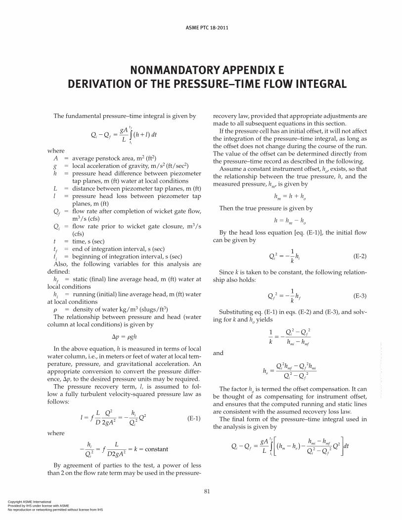
ASME PTC 18-2011

81

NONmANdATORy APPENdIX EdERIVATION OF THE PRESSURE–TImE FlOW INTEGRAl

The fundamental pressure–time integral is given by

Q QgA

Lh l dti f

t

t

i

f

2 5 1( )∫where

A 5 average penstock area, m2 (ft2)g 5 local acceleration of gravity, m/s2 (ft/sec2)h 5 pressure head difference between piezometer

tap planes, m (ft) water at local conditionsL 5 distance between piezometer tap planes, m (ft)l 5 pressure head loss between piezometer tap

planes, m (ft) Qf 5 flow rate after completion of wicket gate flow,

m3/s (cfs)Qi 5 flow rate prior to wicket gate closure, m3/s

(cfs)t 5 time, s (sec)tf 5 end of integration interval, s (sec)ti 5 beginning of integration interval, s (sec)Also, the following variables for this analysis are

defined:hf 5 static (final) line average head, m (ft) water at

local conditionshi 5 running (initial) line average head, m (ft) water

at local conditions 5 density of water kg/m3 (slugs/ft3)The relationship between pressure and head (water

column at local conditions) is given by

p 5 gh

In the above equation, h is measured in terms of local water column, i.e., in meters or feet of water at local tem-perature, pressure, and gravitational acceleration. An appropriate conversion to convert the pressure differ-ence, p, to the desired pressure units may be required.

The pressure recovery term, l, is assumed to fol-low a fully turbulent velocity-squared pressure law as follows:

l fL

D

Q

gA

h

QQi

i

5 522

2 22

2 (E-1)

where

2 5 5 5h

Qf

L

D gAki

i2 22

constant

By agreement of parties to the test, a power of less than 2 on the flow rate term may be used in the pressure-

recovery law, provided that appropriate adjustments are made to all subsequent equations in this section.

If the pressure cell has an initial offset, it will not affect the integration of the pressure–time integral, as long as the offset does not change during the course of the run. The value of the offset can be determined directly from the pressure–time record as described in the following.

Assume a constant instrument offset, ho, exists, so that the relationship between the true pressure, h, and the measured pressure, hm, is given by

hm 5 h 1ho

Then the true pressure is given by

h 5 hm 2ho

By the head loss equation [eq. (E-1)], the initial flow can be given by

Q

khi i

2 152 (E-2)

Since k is taken to be constant, the following relation-ship also holds:

Q

khf f

2 152 (E-3)

Substituting eq. (E-1) in eqs. (E-2) and (E-3), and solv-ing for k and ho yields

1 2 2

k

Q Q

h hi f

mi mf

522

2

and

hQ h Q h

Q Qoi mf f mi

i f

52

2

2 2

2 2

The factor ho is termed the offset compensation. It can be thought of as compensating for instrument offset, and ensures that the computed running and static lines are consistent with the assumed recovery loss law.

The final form of the pressure–time integral used in the analysis is given by

Q QgA

Lh h

h h

Q QQ dti f m o

mi mf

i ft

t

i

f

2 5 2 22

2( )

∫ 2 2

2


--`,`,,`,`,``,,`,````,,`,````-`-`,,`,,`,`,,`---

82

INTENTIONAlly lEFT BlANK


--`,`,,`,`,``,,`,````,,`,````-`-`,,`,,`,`,,`---



--`,`,,`,`,``,,`,````,,`,````-`-`,,`,,`,`,,`---

ASME PTC 18-2011

c01811Copyright ASME International Provided by IHS under license with ASME No reproduction or networking permitted without license from IHS

--`,`,,`,`,``,,`,````,,`,````-`-`,,`,,`,`,,`---

asme ptc 18-2011-hydraulic turbines and pump-turbines-performance test codes

Documents