aspects of quantum game theory · quantum game theory is an exciting new topic that combines the...
TRANSCRIPT

Aspects of Quantum Game Theory
by
Adrian P. Flitney
B.Sc. Honours (Physics), University of Tasmania, Australia, 1983
Thesis submitted for the degree of
Doctor of Philosophy
in
Department of Electrical and Electronic Engineering,
Faculty of Engineering, Computer and Mathematical Sciences
The University of Adelaide, Australia
January, 2005

c© 2005
Adrian P. Flitney
All Rights Reserved

Contents
Heading Page
Contents iii
Abstract ix
Statement of Originality xi
Acknowledgments xiii
Thesis Conventions xv
Publications xvii
List of Figures xix
List of Tables xxiii
Chapter 1. Motivation and Layout of the Thesis 1
1.1 Background and motivation . . . . . . . . . . . . . . . . . . . . . . . . . . 2
1.2 Layout of thesis and original contributions . . . . . . . . . . . . . . . . . . 3
Chapter 2. Introduction to Quantum Games 7
2.1 Game theory . . . . . . . . . . . . . . . . . . . . . . . . . . . . . . . . . . 8
2.1.1 Background . . . . . . . . . . . . . . . . . . . . . . . . . . . . . . . 8
2.1.2 Basic ideas and terminology . . . . . . . . . . . . . . . . . . . . . . 8
2.1.3 An example: the Prisoners’ Dilemma . . . . . . . . . . . . . . . . . 11
2.2 Quantum game theory: the idea . . . . . . . . . . . . . . . . . . . . . . . . 12
2.2.1 Quantum Penny Flip . . . . . . . . . . . . . . . . . . . . . . . . . . 12
2.2.2 A general prescription . . . . . . . . . . . . . . . . . . . . . . . . . 13
2.3 Eisert’s model for 2 × 2 quantum games . . . . . . . . . . . . . . . . . . . 14
2.4 Larger strategic spaces . . . . . . . . . . . . . . . . . . . . . . . . . . . . . 19
Page iii
Contents
2.5 Other models . . . . . . . . . . . . . . . . . . . . . . . . . . . . . . . . . . 20
2.6 Summary . . . . . . . . . . . . . . . . . . . . . . . . . . . . . . . . . . . . 22
Chapter 3. Quantum Version of the Monty Hall Problem 23
3.1 The Monty Hall problem . . . . . . . . . . . . . . . . . . . . . . . . . . . . 24
3.2 Quantization scheme . . . . . . . . . . . . . . . . . . . . . . . . . . . . . . 24
3.3 Results . . . . . . . . . . . . . . . . . . . . . . . . . . . . . . . . . . . . . . 27
3.3.1 Unentangled initial state . . . . . . . . . . . . . . . . . . . . . . . . 27
3.3.2 Maximally entangled initial state . . . . . . . . . . . . . . . . . . . 29
3.4 Summary . . . . . . . . . . . . . . . . . . . . . . . . . . . . . . . . . . . . 30
Chapter 4. Quantum Truel 31
4.1 Introduction . . . . . . . . . . . . . . . . . . . . . . . . . . . . . . . . . . . 32
4.2 The classical truel . . . . . . . . . . . . . . . . . . . . . . . . . . . . . . . . 32
4.3 Quantization scheme . . . . . . . . . . . . . . . . . . . . . . . . . . . . . . 36
4.4 Quantum duels . . . . . . . . . . . . . . . . . . . . . . . . . . . . . . . . . 38
4.5 Quantum truels . . . . . . . . . . . . . . . . . . . . . . . . . . . . . . . . . 39
4.5.1 One- and two-shot truel . . . . . . . . . . . . . . . . . . . . . . . . 43
4.6 Quantum N -uels . . . . . . . . . . . . . . . . . . . . . . . . . . . . . . . . 45
4.7 Classical-quantum correspondence . . . . . . . . . . . . . . . . . . . . . . . 46
4.8 Summary . . . . . . . . . . . . . . . . . . . . . . . . . . . . . . . . . . . . 47
Chapter 5. Advantage of a Quantum Player Over a Classical Player 49
5.1 Introduction . . . . . . . . . . . . . . . . . . . . . . . . . . . . . . . . . . . 50
5.2 Miracle moves . . . . . . . . . . . . . . . . . . . . . . . . . . . . . . . . . . 50
5.3 Critical entanglements in 2 × 2 games . . . . . . . . . . . . . . . . . . . . . 53
5.3.1 Prisoners’ Dilemma . . . . . . . . . . . . . . . . . . . . . . . . . . . 53
5.3.2 Chicken . . . . . . . . . . . . . . . . . . . . . . . . . . . . . . . . . 55
5.3.3 Deadlock . . . . . . . . . . . . . . . . . . . . . . . . . . . . . . . . . 57
5.3.4 Stag Hunt . . . . . . . . . . . . . . . . . . . . . . . . . . . . . . . . 58
5.3.5 Battle of the Sexes . . . . . . . . . . . . . . . . . . . . . . . . . . . 60
5.4 Extensions . . . . . . . . . . . . . . . . . . . . . . . . . . . . . . . . . . . . 61
5.5 Summary . . . . . . . . . . . . . . . . . . . . . . . . . . . . . . . . . . . . 62
Page iv

Contents
Chapter 6. Decoherence in Quantum Games 65
6.1 Introduction . . . . . . . . . . . . . . . . . . . . . . . . . . . . . . . . . . . 66
6.2 Decoherence in Meyer’s quantum Penny Flip . . . . . . . . . . . . . . . . . 68
6.3 Decoherence in the Eisert scheme . . . . . . . . . . . . . . . . . . . . . . . 69
6.3.1 The model . . . . . . . . . . . . . . . . . . . . . . . . . . . . . . . . 69
6.3.2 Prisoners’ Dilemma . . . . . . . . . . . . . . . . . . . . . . . . . . . 71
6.3.3 Chicken . . . . . . . . . . . . . . . . . . . . . . . . . . . . . . . . . 72
6.3.4 Battle of the Sexes . . . . . . . . . . . . . . . . . . . . . . . . . . . 72
6.3.5 General remarks on 2 × 2 games . . . . . . . . . . . . . . . . . . . . 73
6.4 Summary and open questions . . . . . . . . . . . . . . . . . . . . . . . . . 74
Chapter 7. Quantum Parrondo’s Games 77
7.1 Introduction . . . . . . . . . . . . . . . . . . . . . . . . . . . . . . . . . . . 78
7.2 Classical Parrondo’s games . . . . . . . . . . . . . . . . . . . . . . . . . . . 79
7.2.1 Capital-dependent games . . . . . . . . . . . . . . . . . . . . . . . . 79
7.2.2 History-dependent games . . . . . . . . . . . . . . . . . . . . . . . . 79
7.2.3 Other classical Parrondo’s games . . . . . . . . . . . . . . . . . . . 81
7.3 Quantum Parrondo’s games . . . . . . . . . . . . . . . . . . . . . . . . . . 82
7.3.1 Position-dependent games . . . . . . . . . . . . . . . . . . . . . . . 82
7.3.2 History-dependent games . . . . . . . . . . . . . . . . . . . . . . . . 84
7.4 New results for a quantum history-dependent game . . . . . . . . . . . . . 88
7.5 Other quantum Parrondian behaviour . . . . . . . . . . . . . . . . . . . . . 91
7.6 Summary . . . . . . . . . . . . . . . . . . . . . . . . . . . . . . . . . . . . 91
Chapter 8. Quantum Walks with History Dependence 93
8.1 Introduction . . . . . . . . . . . . . . . . . . . . . . . . . . . . . . . . . . . 94
8.1.1 Motivation . . . . . . . . . . . . . . . . . . . . . . . . . . . . . . . . 94
8.1.2 Single coin quantum walk . . . . . . . . . . . . . . . . . . . . . . . 95
8.2 History-dependent multi-coin quantum walk . . . . . . . . . . . . . . . . . 96
8.3 Results and discussion . . . . . . . . . . . . . . . . . . . . . . . . . . . . . 98
8.4 Quantum Parrondo effect . . . . . . . . . . . . . . . . . . . . . . . . . . . . 99
8.5 Summary . . . . . . . . . . . . . . . . . . . . . . . . . . . . . . . . . . . . 103
Page v
Contents
Chapter 9. Some Ideas on Quantum Cellular Automata 105
9.1 Background and motivation . . . . . . . . . . . . . . . . . . . . . . . . . . 106
9.1.1 Classical cellular automata . . . . . . . . . . . . . . . . . . . . . . . 106
9.1.2 Conway’s game of Life . . . . . . . . . . . . . . . . . . . . . . . . . 106
9.1.3 Quantum cellular automata . . . . . . . . . . . . . . . . . . . . . . 108
9.2 Semi-quantum Life . . . . . . . . . . . . . . . . . . . . . . . . . . . . . . . 110
9.2.1 The idea . . . . . . . . . . . . . . . . . . . . . . . . . . . . . . . . . 110
9.2.2 A first model . . . . . . . . . . . . . . . . . . . . . . . . . . . . . . 111
9.2.3 A semi-quantum model . . . . . . . . . . . . . . . . . . . . . . . . . 114
9.2.4 Discussion . . . . . . . . . . . . . . . . . . . . . . . . . . . . . . . . 115
9.3 Summary . . . . . . . . . . . . . . . . . . . . . . . . . . . . . . . . . . . . 116
Chapter 10.Conclusions and Future Directions 121
10.1 New quantum models of classical games . . . . . . . . . . . . . . . . . . . 122
10.1.1 Monty Hall problem—Chapter 3 . . . . . . . . . . . . . . . . . . . . 122
10.1.2 Duels and truels—Chapter 4 . . . . . . . . . . . . . . . . . . . . . . 123
10.1.3 Future directions . . . . . . . . . . . . . . . . . . . . . . . . . . . . 125
10.2 Quantum 2 × 2 games . . . . . . . . . . . . . . . . . . . . . . . . . . . . . 126
10.2.1 A quantum player versus a classical player—Chapter 5 . . . . . . . 126
10.2.2 Decoherence in quantum games—Chapter 6 . . . . . . . . . . . . . 127
10.2.3 Future directions . . . . . . . . . . . . . . . . . . . . . . . . . . . . 128
10.3 Quantum Parrondo’s games—Chapter 7 . . . . . . . . . . . . . . . . . . . 129
10.3.1 Capital- or position-dependent Parrondo’s games . . . . . . . . . . 129
10.3.2 History-dependent Parrondo’s games . . . . . . . . . . . . . . . . . 130
10.3.3 Future directions . . . . . . . . . . . . . . . . . . . . . . . . . . . . 131
10.4 Quantum walks—Chapter 8 . . . . . . . . . . . . . . . . . . . . . . . . . . 131
10.4.1 History-dependent quantum walk . . . . . . . . . . . . . . . . . . . 131
10.4.2 Future directions . . . . . . . . . . . . . . . . . . . . . . . . . . . . 132
10.5 Quantum cellular automata—Chapter 9 . . . . . . . . . . . . . . . . . . . 133
10.5.1 One-dimensional quantum cellular automata . . . . . . . . . . . . . 133
10.5.2 Semi-quantum version of the game of Life . . . . . . . . . . . . . . 134
10.5.3 Future directions . . . . . . . . . . . . . . . . . . . . . . . . . . . . 134
10.6 Final comments . . . . . . . . . . . . . . . . . . . . . . . . . . . . . . . . . 134
Page vi

Contents
Appendix A. Software routines 137
A.1 Quantum 2 × 2 games—Chapters 5 and 6 . . . . . . . . . . . . . . . . . . 138
A.2 Classical Parrondo’s games—Chapter 7 . . . . . . . . . . . . . . . . . . . . 139
A.2.1 Capital-dependent game—Section 7.2.1 . . . . . . . . . . . . . . . . 139
A.2.2 History-dependent game—Section 7.2.2 . . . . . . . . . . . . . . . . 144
A.3 Quantum walks—Section 7.3.1 and Chapter 8 . . . . . . . . . . . . . . . . 148
A.4 Quantum cellular automata—Chapter 9 . . . . . . . . . . . . . . . . . . . 158
A.4.1 One-dimensional QCA—Section 9.1.3 . . . . . . . . . . . . . . . . . 158
A.4.2 Semi-quantum Life—Section 9.2 . . . . . . . . . . . . . . . . . . . . 162
Bibliography 167
Acronyms 179
Symbols Used 181
Index 185
Resume 187
Page vii

Page viii

Abstract
Quantum game theory is an exciting new topic that combines the physical behaviour of
information in quantum mechanical systems with game theory, the mathematical descrip-
tion of conflict and competition situations, to shed new light on the fields of quantum
control and quantum information. This thesis presents quantizations of some classic
game-theoretic problems, new results in existing quantization schemes for two player, two
strategy non-zero sum games, and in quantum versions of Parrondo’s games, where the
combination of two losing games can result in a winning game. In addition, quantum
cellular automata and quantum walks are discussed, with a history-dependent quantum
walk being presented.
Page ix

Page x

Statement of Originality
This work contains no material that has been accepted for the award of any other degree
or diploma in any university or other tertiary institution and, to the best of my knowledge
and belief, contains no material previously published or written by another person, except
where due reference has been made in the text.
I give consent to this copy of the thesis, when deposited in the University Library, being
available for loan, photocopying, and dissemination through the digital thesis collection.
4th January, 2005
Signed Date
Page xi

Page xii

Acknowledgments
A work of this magnitude could not possibly have been undertaken without scorning the
advice of too many people to mention here. George W. Bush and Rupert Murdoch are
just two of the people whose advice was not even sort, nor did they provide any funding.
However, generous funding was provided by the GTECH Corporation with help from the
SA Lotteries Commission. Travel funding was provided by The University of Adelaide
postgraduate travel award, the D. R. Stranks postgraduate travel scholarship and the
Department of Electrical and Electronic Engineering at The University of Adelaide. The
support, direction and encouragement of my supervisor, A/Prof. Derek Abbott is grate-
fully acknowledged. I would also like to thank various colleagues and collaborators for
useful discussions and help with various parts of this work: Prof. Jens Eisert of Potsdam
University, Prof. Neil F. Johnson of Oxford University, Wanli Li of Princeton University,
Prof. David Meyer of the University of California San Diego (UCSD), Joseph Ng of the
University of Queensland, Dr. Arun Pati of the University of Bangor, and a number of
others with whom I spoke at conferences and during interstate or overseas visits. I would
like to thank my fellow students at the Centre for Biomedical Engineering and those I
spent time with at the Physics Departments at Melbourne, Oxford and Potsdam Univer-
sities. Finally, I would like to thank my family and friends, without whom life would be
impossible.
—Adrian Flitney
“Returning home I read a book on Physics. I don’t understand it very well . . . Why
isn’t nature clearer and more directly comprehensible?”
—Shin’ichiro Tomonaga, Nobel prize winner in Physics, 1965
Page xiii
Page xiv

Thesis Conventions
Typesetting. This thesis is typeset using LATEX2e software. Plots were generated by
Mathematica 4.1. CorelDRAW 7.467 was used to generate some of the schematic
diagrams, while the remainder were generated with standard LATEX picture com-
mands.
Spelling. Australian English spelling has been adopted throughout, as defined by the
Macquarie English Dictionary (A. Delbridge (ed.) Macquarie Library, North Ryde,
NSW, Australia, 2001). Where more than one spelling variant is permitted such as
biassing or biasing and infra-red or infrared the option with the fewest characters
has been chosen.
Mathematics. The International Standards Organization has established the recognized
conventions for typesetting mathematics. The most important points are given
below.
1. Equations are treated as part of the text and include the appropriate punctu-
ation.
2. Simple variables are represented by italic letters, e.g., x, y or z.
3. Vectors are written in bold face italic, e.g., B or π.
4. Superscripts or subscripts that are descriptions and not variables are in upright
font, e.g., kA where A stands for Alice as opposed to ki where i = 1, . . . , n.
Referencing. The Harvard style is used for referencing and citation.
Page xv

Page xvi
Publications
FLITNEY-A. P and Abbott-D (2005). Quantum games with decoherence, J. Phys. A, 38,
449–59.
FLITNEY-A. P and Abbott-D (2004c). A semi-quantum version of the game of Life, in A. S.
Nowak and K. Szajowski (eds.), Advances in Dynamic Games: Applications to Economics,
Finance, Optimization and Stochastic Control (Proc. 9th Int. Symp. on Dynamic Games
and Applications, Adelaide, Australia, Dec. 2000), Birkhauser, Boston, pp. 667–79.
FLITNEY-A. P and Abbott-D (2004b). Quantum two and three person duels, J. Optics B,
6, S860–6.
FLITNEY-A. P and Abbott-D (2004a). Decoherence in quantum games, in P. Heszler and
D. Abbott and J. R. Gea-Banacloche and P. R. Hemmer (eds.), Proc. SPIE Symp. on
Fluctuations and Noise in Photonics and Quantum Optics II, Vol. 5468, Maspalomas,
Spain, pp. 313–21.
FLITNEY-A. P, Abbott-D and Johnson-N. F (2004). Quantum walks with history depen-
dence, J. Phys. A, 30, 7581–91.
FLITNEY-A. P and Abbott-D (2003c). Quantum models of Parrondo’s games, Physica A,
324, 152–6.
FLITNEY-A. P and Abbott-D (2003b). Quantum duels and truels, in D. Abbott and
J. H. Shapiro and Y. Yamamoto (eds.), Proc. SPIE Symp. on Fluctuations and Noise in
Photonics and Quantum Optics, Vol. 5111, Santa Fe, New Mexico, pp. 358–69.
FLITNEY-A. P and Abbott-D (2003a). Advantage of a quantum player against a classical
one in 2 × 2 quantum games, Proc. Roy. Soc. (Lond.) A, 459, 2463–74.
FLITNEY-A. P and Abbott-D (2002c). Quantum version of the Monty Hall problem, Phys.
Rev. A, 65, 062318.
FLITNEY-A. P and Abbott-D (2002b). Quantum models of Parrondo’s games, in D. K.
Sood and A. P. Malshe and R. Maeda (eds.), Proc. SPIE Nano- and Microtechnology:
Materials, Processes, Packaging and Systems Conf., Vol. 4936, Melbourne, Australia, pp.
58–64.
FLITNEY-A. P and Abbott-D (2002a). An introduction to quantum game theory, Fluct.
Noise Lett., 2, R175–87.
Page xvii

Publications
FLITNEY-A. P, Ng-J and Abbott-D (2002). Quantum Parrondo’s games, Physica A, 314,
35–42.
Page xviii
List of Figures
Figure Page
1.1 Layout of the thesis . . . . . . . . . . . . . . . . . . . . . . . . . . . . . . . 5
2.1 Quantum Penny Flip . . . . . . . . . . . . . . . . . . . . . . . . . . . . . . 13
2.2 Protocol for a two person quantum game . . . . . . . . . . . . . . . . . . . 14
2.3 Protocol for an N -person quantum game . . . . . . . . . . . . . . . . . . . 19
4.1 Schematic of a truel . . . . . . . . . . . . . . . . . . . . . . . . . . . . . . . 33
4.2 Game tree for a duel between Alice and Bob . . . . . . . . . . . . . . . . . 35
4.3 Game tree for a one shot truel . . . . . . . . . . . . . . . . . . . . . . . . . 35
4.4 Game tree for a two-shot truel . . . . . . . . . . . . . . . . . . . . . . . . . 36
4.5 Quantum circuit for Alice “firing” at Bob . . . . . . . . . . . . . . . . . . . 38
4.6 Expectation of Alice’s payoff in a two shot quantum duel as a function of
phases . . . . . . . . . . . . . . . . . . . . . . . . . . . . . . . . . . . . . . 40
4.7 Expectation value of Alice’s payoff in a repeated quantum duel . . . . . . . 40
4.8 Improvement in Alice’s payoff in a two shot quantum duel if she chooses
to shoot in the air on her second shot . . . . . . . . . . . . . . . . . . . . . 41
4.9 Alice’s preferred strategy in a one shot quantum truel with Alice being the
poorest shot . . . . . . . . . . . . . . . . . . . . . . . . . . . . . . . . . . . 44
4.10 Alice’s preferred strategy in a two shot quantum truel with Alice being the
poorest shot . . . . . . . . . . . . . . . . . . . . . . . . . . . . . . . . . . . 45
4.11 Alice and Bob’s preferred strategy in a two shot quantum truel with Bob
being the poorest shot . . . . . . . . . . . . . . . . . . . . . . . . . . . . . 46
4.12 Alice’s preferred strategy in a one-shot quantum truel with decoherence . . 48
Page xix
List of Figures
5.1 Expected payoffs in quantum Prisoners’ Dilemma as a function of entan-
glement . . . . . . . . . . . . . . . . . . . . . . . . . . . . . . . . . . . . . 54
5.2 Payoffs as a function of entanglement in quantum Prisoners’ Dilemma when
Alice defects . . . . . . . . . . . . . . . . . . . . . . . . . . . . . . . . . . . 54
5.3 Expected payoffs in quantum Chicken as a function of entanglement . . . . 57
5.4 Payoffs as a function of entanglement in quantum Chicken when Alice defects 58
5.5 Payoffs as a function of entanglement in quantum Deadlock when Alice
defects . . . . . . . . . . . . . . . . . . . . . . . . . . . . . . . . . . . . . . 59
5.6 Payoffs as a function of entanglement in quantum Stag Hunt when Alice
defects . . . . . . . . . . . . . . . . . . . . . . . . . . . . . . . . . . . . . . 60
5.7 Expected payoffs in quantum Battle of the Sexes as a function of entanglement 61
6.1 Flow of information in a quantum game with decoherence . . . . . . . . . . 71
6.2 Payoffs in quantum Prisoners’ Dilemma with decoherence . . . . . . . . . . 72
6.3 Payoffs in quantum Chicken with decoherence . . . . . . . . . . . . . . . . 73
6.4 Payoffs in quantum Battle of the Sexes with decoherence . . . . . . . . . . 74
6.5 Payoffs with optimal strategies as a function of decoherence in Prisoners’
Dilemma, Chicken and Battle of the Sexes . . . . . . . . . . . . . . . . . . 75
7.1 Classical capital-dependent Parrondo’s game . . . . . . . . . . . . . . . . . 80
7.2 Results for a classical capital-dependent Parrondo game for various sequences 80
7.3 History-dependent Parrondo’s games . . . . . . . . . . . . . . . . . . . . . 81
7.4 Results for a classical history-dependent Parrondo game for various sequences 82
7.5 Tilted sawtooth potential . . . . . . . . . . . . . . . . . . . . . . . . . . . . 84
7.6 Expected gain for a quantum position-dependent Parrondo game for vari-
ous sequences . . . . . . . . . . . . . . . . . . . . . . . . . . . . . . . . . . 85
7.7 Expected gain for a quantum position-dependent Parrondo game as a func-
tion of game mixture . . . . . . . . . . . . . . . . . . . . . . . . . . . . . . 86
7.8 Expected gain for a quantum position-dependent Parrondo game for vari-
ous parameter values in the potentials . . . . . . . . . . . . . . . . . . . . 86
7.9 Quantum circuit for a history-dependent Parrondo game . . . . . . . . . . 87
Page xx
List of Figures
7.10 Quantum circuits for various periodic sequences of games A and B in a
history-dependent Parrondo game . . . . . . . . . . . . . . . . . . . . . . . 89
8.1 Probability density distribution for an unbiased quantum walk . . . . . . . 96
8.2 Probability density distributions for 2-, 3- and 4-coin unbiased quantum
walks . . . . . . . . . . . . . . . . . . . . . . . . . . . . . . . . . . . . . . . 98
8.3 Expectation value and standard deviation of position for a 3-coin quantum
walk for various parameter values . . . . . . . . . . . . . . . . . . . . . . . 100
8.4 Probability density distribution for biased 3-coin quantum walks . . . . . . 100
8.5 An example of a Parrondo effect in a 3-coin history-dependent quantum walk102
9.1 One-dimensional cellular automaton . . . . . . . . . . . . . . . . . . . . . . 107
9.2 One-dimensional partitioned cellular automata . . . . . . . . . . . . . . . . 107
9.3 Simple patterns in Conway’s Life . . . . . . . . . . . . . . . . . . . . . . . 109
9.4 A Life glider . . . . . . . . . . . . . . . . . . . . . . . . . . . . . . . . . . . 110
9.5 One-dimensional quantum cellular automaton . . . . . . . . . . . . . . . . 110
9.6 Destructive interference in semi-quantum Life . . . . . . . . . . . . . . . . 117
9.7 Wicks in semi-quantum Life . . . . . . . . . . . . . . . . . . . . . . . . . . 118
9.8 A stable loop in semi-quantum Life . . . . . . . . . . . . . . . . . . . . . . 118
9.9 A stable boundary in semi-quantum Life . . . . . . . . . . . . . . . . . . . 119
9.10 A collision between a glider and an anti-glider in semi-quantum Life . . . . 119
Page xxi

Page xxii

List of Tables
Table Page
3.1 Monty Hall problem . . . . . . . . . . . . . . . . . . . . . . . . . . . . . . 24
5.1 Payoff matrices for various 2 × 2 games . . . . . . . . . . . . . . . . . . . . 51
5.2 Critical entanglements for 2 × 2 quantum games . . . . . . . . . . . . . . . 62
7.1 Expected payoffs per qubit for various sequences in a history-dependent
Parrondo game . . . . . . . . . . . . . . . . . . . . . . . . . . . . . . . . . 91
Page xxiii


Page xxiv

Chapter 1
Motivation and Layout ofthe Thesis
THIS chapter provides a brief background of, and motivation for, the
study of quantum games. It gives a guide to the contents of the
thesis and a list of the important original contributions.
Page 1
1.1 Background and motivation
“Landauer based his research on a simple rule: information is physical. That is,
information is registered by physical systems such as strands of DNA, neurons and
transistors; in turn the ways in which systems such as cells, brains and computers
can process information is governed by the laws of physics. Landauer’s work showed
that the apparently simple and unproblematic statement of the physical nature of
information had profound consequences.”
—Seth Lloyd on Rolf Laundauer (Lloyd 1999)
1.1 Background and motivation
Game theory is the mathematical language of competitive scenarios where the outcome is
contingent upon interacting strategies of two or more agents with conflicting, or at best
self-interested, motivations. Originally developed for use in economics by von Neumann
and Morgenstein (1944), with important contributions by Nash (1950), it has now found a
wide variety of uses in the social sciences, biology, computer science, international relations
and, more recently, physics (Abbott et al. 2002).
Computers that exploit the inherent features of quantum mechanics, such as superposi-
tion and entanglement, are known as quantum computers [see, for example, Eisert and
Wohl (2004)]. The rise of interest in quantum computing has brought with it increasing
attention to the field of quantum information, the study of information processing tasks
using quantum systems (Nielsen and Chuang 2000). At the intersection of game theory
and quantum information is the new field of quantum game theory, created in 1999 when
two groups independently had the idea of applying the rules of quantum mechanics to
game theory (Eisert et al. 1999, Meyer 1999). Replacing the classical probabilities of
game theory by quantum amplitudes creates the possibility of new effects resulting from
superposition or entanglement. To date quantum game theory has concentrated on ob-
serving these new effects amongst the traditional settings of game theory, but ultimately
quantum game-theoretic techniques could be used in quantum communication (Brandt
1998) or quantum computing (Lee and Johnson 2002a) protocols. For example, quantum
communication in competition with an eavesdropper (Gisin and Huttner 1997), optimal
cloning (Werner 1998), or quantum gambling (Goldenberg et al. 1999) can be consid-
ered as games. There has been a proposal to use quantum game theory in a quantum
teleportation protocol (Pirandola 2004) and in quantum state estimation and quantum
cloning (Lee and Johnson 2003b). A review of suggested applications of quantum games
Page 2
Chapter 1 Motivation and Layout of the Thesis
is given by Piotrowski and SÃladowski (2004a). In the meantime quantum games have
stimulated popular discussion (Peterson 1999, Collins 2000, Klarreich 2001b, Cho 2002,
Lee and Johnson 2002b, Siegfried 2003a, Siegfried 2003b) and their study adds to our
understanding of quantum information theory.
This thesis is concerned with developing the topic of quantum game theory. Only theoret-
ical aspects are considered in this thesis—the details of the physical systems are omitted.
The thesis is written for a readership with familiarity with basic quantum mechanics.
Some necessary background on game theory is given in Chapter 2.
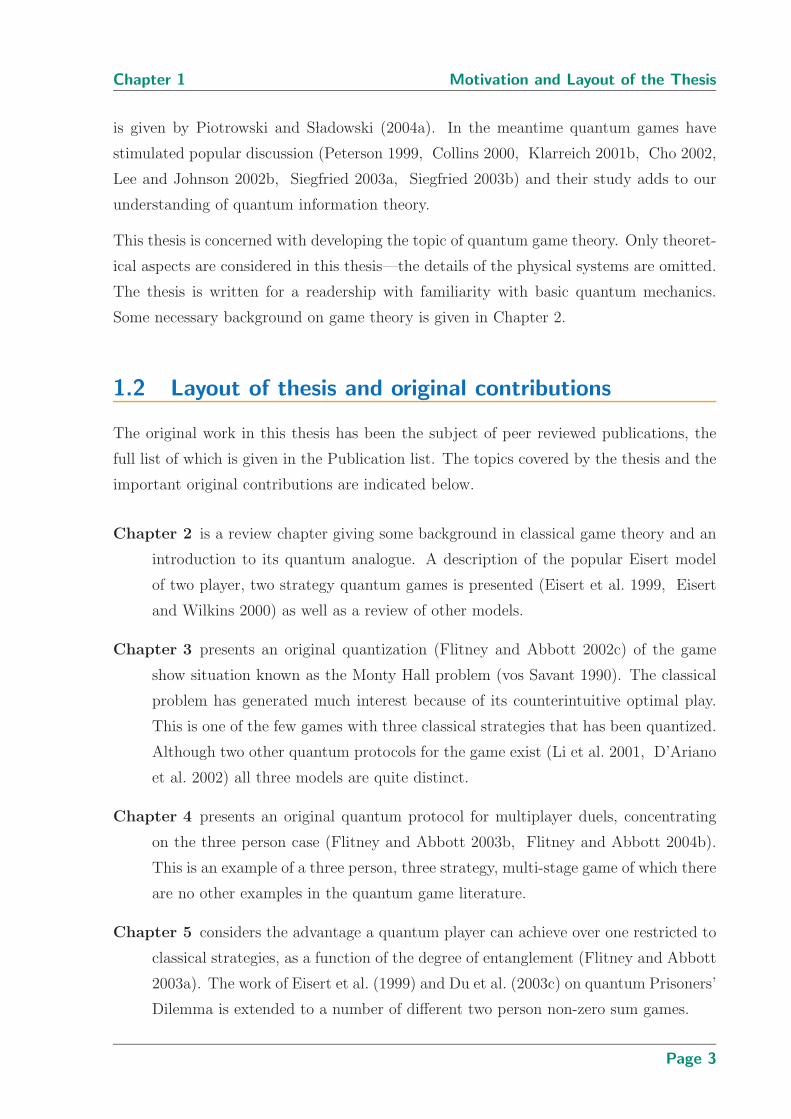
1.2 Layout of thesis and original contributions
The original work in this thesis has been the subject of peer reviewed publications, the
full list of which is given in the Publication list. The topics covered by the thesis and the
important original contributions are indicated below.
Chapter 2 is a review chapter giving some background in classical game theory and an
introduction to its quantum analogue. A description of the popular Eisert model
of two player, two strategy quantum games is presented (Eisert et al. 1999, Eisert
and Wilkins 2000) as well as a review of other models.
Chapter 3 presents an original quantization (Flitney and Abbott 2002c) of the game
show situation known as the Monty Hall problem (vos Savant 1990). The classical
problem has generated much interest because of its counterintuitive optimal play.
This is one of the few games with three classical strategies that has been quantized.
Although two other quantum protocols for the game exist (Li et al. 2001, D’Ariano
et al. 2002) all three models are quite distinct.
Chapter 4 presents an original quantum protocol for multiplayer duels, concentrating
on the three person case (Flitney and Abbott 2003b, Flitney and Abbott 2004b).
This is an example of a three person, three strategy, multi-stage game of which there
are no other examples in the quantum game literature.
Chapter 5 considers the advantage a quantum player can achieve over one restricted to
classical strategies, as a function of the degree of entanglement (Flitney and Abbott
2003a). The work of Eisert et al. (1999) and Du et al. (2003c) on quantum Prisoners’
Dilemma is extended to a number of different two person non-zero sum games.
Page 3
1.2 Layout of thesis and original contributions
Chapter 6 examines how decoherence can be incorporated in quantum games of the
Eisert scheme (Flitney and Abbott 2004a, Flitney and Abbott 2005). In the existing
literature there is a single publication on decoherence in quantum games and this
only considers Prisoners’ Dilemma (Chen et al. 2003b). This thesis gives a model
for decoherence in a more general quantum game setting and considers a number
of two player, two strategy games. The advantage a quantum player has over a
classical player is used as a measure of the “quantum-ness” of the games.
Chapter 7 gives an introduction to classical and quantum Parrondo’s games (Flitney
and Abbott 2003c). Parrondo’s games occur when a mixture of two losing games
can result in a winning game (Harmer and Abbott 1999a). A quantum analogy to
a capital-dependent Parrondo’s game exists (Meyer and Blumer 2002a). Here, new
results are presented for a history-dependent quantum Parrondo game (Flitney et
al. 2002) as well as further results for the earlier model (Flitney and Abbott 2002b).
The model of the history-dependent quantum Parrondo game was first formulated
in 2000 by Ng and Abbott (2004) but the calculations developed in this thesis are
original.
Chapter 8 discusses quantum walks, the quantum analogue of classical random walks.
A new multi-coin model of a quantum walk with history dependence is presented
and its features are discussed (Flitney et al. 2004). Introduction of a bias through
the history dependence distinguishes our model from existing work on multi-coin
quantum walks (Brun et al. 2003b). The new model can produce another example
of a quantum Parrondo’s game and thus this chapter is an extension of the work
detailed in Chapter 7. The work was carried out in collaboration with Prof. Neil F.
Johnson of the Physics Department, Oxford University.
Chapter 9 gives a brief introduction to quantum cellular automata. A new semi-quantum
version of the John Conway’s famous two-dimensional cellular automata Life (Gard-
ner 1970) is presented and some novel structures in the new model are discussed
(Flitney and Abbott 2004c).
Chapter 10 gives a comprehensive summary of the thesis and possible future directions.
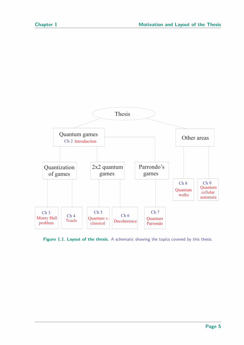
These contributions further the body of knowledge of quantum game theory. The layout
of the material in the thesis is shown in Figure 1.1.
Page 4
Chapter 1 Motivation and Layout of the Thesis
Figure 1.1. Layout of the thesis. A schematic showing the topics covered by this thesis.
Page 5

Page 6

Chapter 2
Introduction to QuantumGames
THIS chapter provides a brief overview of classical game theory and a
list of definitions of game-theoretic terms that occur elsewhere in the
thesis. An introduction to quantum game theory is presented as well
as a review of published ideas in the field. The well known scheme of Eisert
et al. (1999) for two player, two strategy quantum games with entanglement
is discussed. Aspects of this model are the subject of Chapters 5 and 6.
Page 7

2.1 Game theory
2.1 Game theory
2.1.1 Background
Game theory is a tool for rational decision making in conflict situations. It has long
been commonly used in economics, the social sciences and biology to model decision
making situations where the outcomes are contingent upon the interacting strategies of
two or more agents with conflicting, or at best, self-interested motives. There is now
increasing interest in applying game-theoretic techniques in physics. The models are
necessarily idealizations of the physical situations. The need for simplification rules out
the application of game-theoretic techniques to most situations that lay people would call
games, such as chess, where there are simply too many possibilities. The situations of
interest to game theory are those where the agents, or players, can select one of a small
number of options, or strategies. The results of the game, and the corresponding payoffs
to the players, are determined collectively by the strategies of all the agents. The following
section gives formal definitions to the terms and gives a simple example.
2.1.2 Basic ideas and terminology
Definition 2.1 Game: a set of players, a set of rules that specify the possible actions
of the players, and a set of payoff functions giving the rewards to the players for the
various game outcomes, that is, a triple N, Ω, Γ, where N is the number of players,
Ω = S1, . . . , SN with Sj being the set of strategies available to the jth player and
Γ = P1, . . . , PN with Pj being the payoff function for the jth player, j = 1, . . . , N .
Definition 2.2 Payoff or utility: a number that measures the desirability of a partic-
ular game outcome for a player. There is a game outcome associated with each strategy
profile s1, . . . , sN, with sj ∈ Sj, j = 1, . . . , N . Each game outcome is assigned a pay-
off by each player. A mapping from the set of all possible strategy profiles to the real
numbers, Pk : s1, . . . , sN → R, is known as the payoff matrix.
Definition 2.3 Action or move: a choice available to a player.
Definition 2.4 Strategy: a rule that prescribes the action of a player contingent upon
the game situation.
Page 8

Chapter 2 Introduction to Quantum Games
Definition 2.5 Pure strategy: a strategy that specifies a unique move in a given game
position. Unless otherwise specified, the term “strategy” refers to a pure strategy.
Definition 2.6 Mixed strategy: a strategy that uses a randomizing device, such as a
coin, to select amongst alternatives for some or all game positions.
Definition 2.7 Dominant strategy: a strategy that results in a higher payoff than
any alternate strategy against all possible strategic choices by the other player(s). That
is, sk is a dominant strategy for player k if
∀sj, j 6= k, Pk(s1, . . . , sk, . . . sN) ≥ Pk(s1, . . . , s′k, . . . sN) ∀s′k
Definition 2.8 n1 × n2 × . . . × nN game: an N player game where the jth player has
available nj strategies.
Definition 2.9 Zero sum game: a game in which the sum of all the players’ payoffs is
zero regardless of the strategies they choose.
Definition 2.10 Game of perfect information: a game where all the information
about the position, the strategy sets and the payoff functions of the players is known to
all.
Definition 2.11 Symmetric game: one where all agents have the same set of strategies
and identical payoff functions, except for the interchange of roles of the players.
Definition 2.12 Nash equilibrium (NE): a game result from which no player can
improve their payoff by a unilateral change in strategy (Nash 1950, Nash 1951). That is,
the strategy profile s1, . . . , sN is an NE if
∀k, Pk(s1, . . . , sk, . . . , sN) ≥ Pk(s1, . . . , s′k, . . . , sN) ∀s′k
Definition 2.13 Focal point: one amongst several NE that, for psychological reasons,
is particularly compelling.
Definition 2.14 Maximin: a game equilibrium where each player maximizes the min-
imum payoff that they can receive. That is, each player assumes that for any strategy
Page 9
2.1 Game theory
they choose their opponent(s) will respond with the strategy that hurts them the most.
With this expected behaviour the optimal choice is the one that provides the maximum of
the worst case payoffs. This equilibrium makes sense in zero-sum games where there are
purely competitive forces, but fails to take into account possible benefits from cooperation
in other situations.
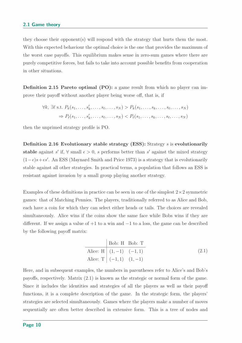
Definition 2.15 Pareto optimal (PO): a game result from which no player can im-
prove their payoff without another player being worse off, that is, if
∀k, ∃ℓ s.t. Pk(s1, . . . , s′k, . . . , sℓ, . . . , sN) > Pk(s1, . . . , sk, . . . , sℓ, . . . , sN)
⇒ Pℓ(s1, . . . , s′k, . . . , sℓ, . . . , sN) < Pℓ(s1, . . . , sk, . . . , sℓ, . . . , sN)
then the unprimed strategy profile is PO.
Definition 2.16 Evolutionary stable strategy (ESS): Strategy s is evolutionarily
stable against s′ if, ∀ small ǫ > 0, s performs better than s′ against the mixed strategy
(1−ǫ)s+ǫs′. An ESS (Maynard Smith and Price 1973) is a strategy that is evolutionarily
stable against all other strategies. In practical terms, a population that follows an ESS is
resistant against invasion by a small group playing another strategy.
Examples of these definitions in practice can be seen in one of the simplest 2×2 symmetric
games: that of Matching Pennies. The players, traditionally referred to as Alice and Bob,
each have a coin for which they can select either heads or tails. The choices are revealed
simultaneously. Alice wins if the coins show the same face while Bobs wins if they are
different. If we assign a value of +1 to a win and −1 to a loss, the game can be described
by the following payoff matrix:
Bob: H Bob: T
Alice: H (1,−1) (−1, 1)
Alice: T (−1, 1) (1,−1)
(2.1)
Here, and in subsequent examples, the numbers in parentheses refer to Alice’s and Bob’s
payoffs, respectively. Matrix (2.1) is known as the strategic or normal form of the game.
Since it includes the identities and strategies of all the players as well as their payoff
functions, it is a complete description of the game. In the strategic form, the players’
strategies are selected simultaneously. Games where the players make a number of moves
sequentially are often better described in extensive form. This is a tree of nodes and
Page 10
Chapter 2 Introduction to Quantum Games
branches, the nodes being game positions labeled by the player who has the move and
the branches labeled by the possible moves of that player. Examples of the extensive
description of a game are given in Chapter 4, however, the strategic form is the one that
shall be used in the majority of this thesis.
In Matching Pennies there are two pure strategies: “show heads” or “show tails.” A
mixed strategy is something like “show heads half the time and tails the other half.” A
casual examination of the game shows that there is no best move, or dominant strategy,
for the players: any option yields a 50% chance of success. For all game results one player
wins and the other looses. Thus the game is zero-sum.
2.1.3 An example: the Prisoners’ Dilemma
One 2 × 2 game that has deservedly received much attention is the Prisoners’ Dilemma
(Rapoport and Chammah 1965). Here, the players’ moves are known as cooperation (C)
or defection (D), for reasons that shall become clear. The payoff matrix is such that there
is a conflict between the NE and the PO outcome. The payoff matrix can be written as
Bob: C Bob: D
Alice: C (3,3) (0,5)
Alice: D (5,0) (1,1)
(2.2)
The game is symmetric and there is a dominant strategy, that of always defecting, since
it gives a better payoff if the other player cooperates (five instead of three) or if the other
player defects (one instead of zero). Where both players have a dominant strategy, this
combination is the NE.
The NE outcome D,D is not such a good one for the players, however, since if they had
both cooperated they would have both received a payoff of three, the PO result. In the
absence of communication or negotiation we have a dilemma between the personal and
the mutual good, some form of which is responsible for much of the misery and conflict
through out the world. Game theory does not have a solution. In a one-off Prisoners’
Dilemma the rational player postulated by the theory should defect. In the real world the
opportunity to play the game repeatedly and the ability to negotiate helps to foster some
degree of cooperation even in pure Prisoners’ Dilemma situations (Axelrod 1981, Axelrod
and Hamilton 1984). There is extensive literature on the Prisoners’ Dilemma and it is
mentioned in any introductory text on game theory (see, for example, Rasmusen (1989)).
Page 11
2.2 Quantum game theory: the idea
2.2 Quantum game theory: the idea
2.2.1 Quantum Penny Flip
One of the simplest gaming devices is that of a two state system such as a coin. If we have
a player than can utilize quantum moves, we can demonstrate how the expanded space of
possible strategies can be turned to advantage. Meyer, in his seminal work on quantum
game theory (Meyer 1999), considered the simple game Penny Flip that consists of the
following: Alice prepares a coin in the heads state and places it in a box where neither
player can see it. Bob can choose to either flip the coin or leave its state unaltered, and
Alice, without knowing Bob’s action, can do likewise. Finally, Bob has a second turn at
the coin. The coin is now examined and Bob wins if it shows heads. A classical coin
clearly gives both players an equal probability of success unless they utilize knowledge of
the other’s psychological bias, and such knowledge is beyond analysis by game theory.1
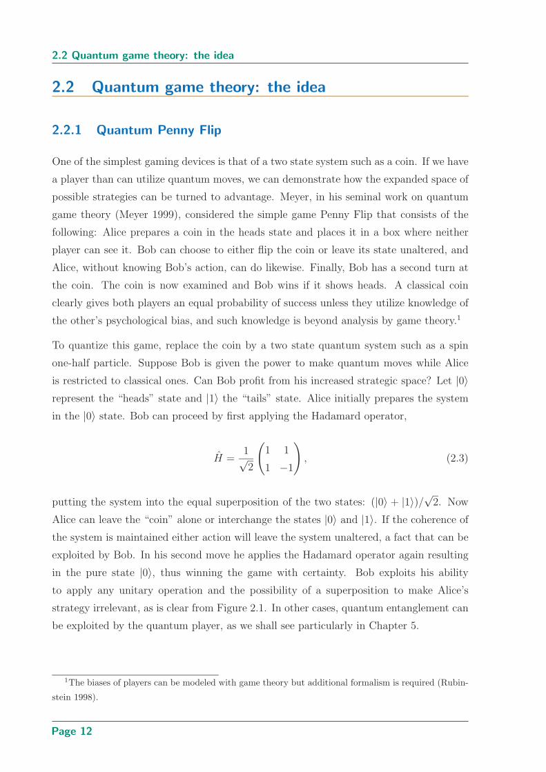
To quantize this game, replace the coin by a two state quantum system such as a spin
one-half particle. Suppose Bob is given the power to make quantum moves while Alice
is restricted to classical ones. Can Bob profit from his increased strategic space? Let |0〉represent the “heads” state and |1〉 the “tails” state. Alice initially prepares the system
in the |0〉 state. Bob can proceed by first applying the Hadamard operator,
H =1√2
(
1 1
1 −1
)
, (2.3)
putting the system into the equal superposition of the two states: (|0〉 + |1〉)/√
2. Now
Alice can leave the “coin” alone or interchange the states |0〉 and |1〉. If the coherence of
the system is maintained either action will leave the system unaltered, a fact that can be
exploited by Bob. In his second move he applies the Hadamard operator again resulting
in the pure state |0〉, thus winning the game with certainty. Bob exploits his ability
to apply any unitary operation and the possibility of a superposition to make Alice’s
strategy irrelevant, as is clear from Figure 2.1. In other cases, quantum entanglement can
be exploited by the quantum player, as we shall see particularly in Chapter 5.
1The biases of players can be modeled with game theory but additional formalism is required (Rubin-
stein 1998).
Page 12

Chapter 2 Introduction to Quantum Games
Figure 2.1. Quantum Penny Flip. The Bloch sphere for the quantum coin in Penny Flip. The coin
starts in the |0〉 state. The quantum player (Bob) is able to apply any rotation, while
the player restricted to classical moves (Alice) can only apply the identity or a bit-flip
(a reflection about the horizontal). Bob exploits his advantage by rotating the qubit
to the horizontal using H making Alice impotent in her move. Since Bob has certain
knowledge of the state of the qubit before his second move, he can again employ H to
rotate back to |0〉.
2.2.2 A general prescription
Where a player has a choice of two moves, the choice can be encoded in a single bit. To
translate this into the quantum realm the bit is replaced by a quantum bit or qubit, which
can be in a linear superposition of the two states. The basis states |0〉 and |1〉 correspond
to the classical moves. The players’ qubits are initially prepared by a referee in a state
to be specified later. We suppose the players apply their chosen strategy using a set of
instruments that can manipulate their qubit while maintaining coherence of the quantum
state. That is, a pure quantum strategy is a local unitary operator acting on the player’s
qubit. After all players have executed their moves the qubits are returned to the referee
who makes a positive operator valued measurement on the set and determines the payoffs
according to the outcome of the measurement. The classical strategies “always play 0”
and “always play 1” are represented by the identity operator I and the bit-flip operator,
F ≡ iσx =
(
0 i
i 0
)
, (2.4)
respectively. The resulting quantum game contains the classical one as a subset. A
description of the formalism of quantum games is given by Lee and Johnson (2003a).
Page 13
2.3 Eisert’s model for 2 × 2 quantum games
|0〉
|0〉⊗ |ψf〉J J†
A
B
-time
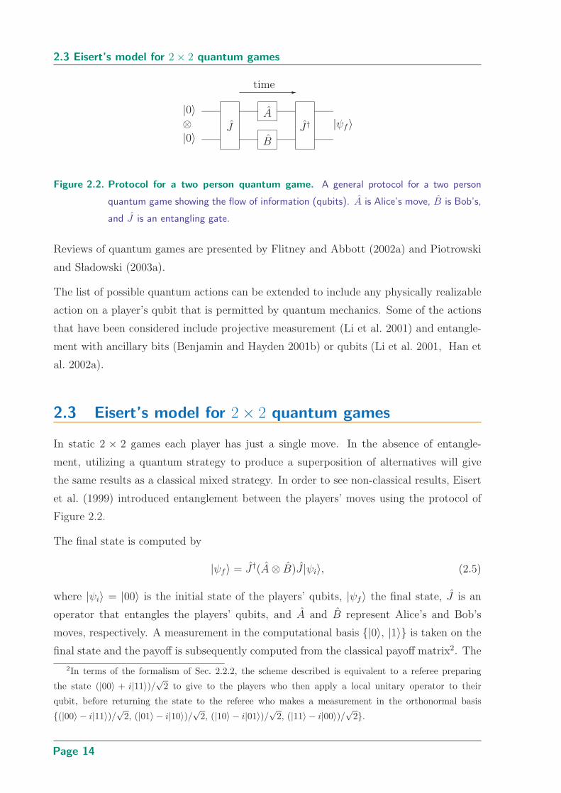
Figure 2.2. Protocol for a two person quantum game. A general protocol for a two person
quantum game showing the flow of information (qubits). A is Alice’s move, B is Bob’s,
and J is an entangling gate.
Reviews of quantum games are presented by Flitney and Abbott (2002a) and Piotrowski
and SÃladowski (2003a).
The list of possible quantum actions can be extended to include any physically realizable
action on a player’s qubit that is permitted by quantum mechanics. Some of the actions
that have been considered include projective measurement (Li et al. 2001) and entangle-
ment with ancillary bits (Benjamin and Hayden 2001b) or qubits (Li et al. 2001, Han et
al. 2002a).
2.3 Eisert’s model for 2 × 2 quantum games
In static 2 × 2 games each player has just a single move. In the absence of entangle-
ment, utilizing a quantum strategy to produce a superposition of alternatives will give
the same results as a classical mixed strategy. In order to see non-classical results, Eisert
et al. (1999) introduced entanglement between the players’ moves using the protocol of
Figure 2.2.
The final state is computed by
|ψf〉 = J†(A ⊗ B)J |ψi〉, (2.5)
where |ψi〉 = |00〉 is the initial state of the players’ qubits, |ψf〉 the final state, J is an
operator that entangles the players’ qubits, and A and B represent Alice’s and Bob’s
moves, respectively. A measurement in the computational basis |0〉, |1〉 is taken on the
final state and the payoff is subsequently computed from the classical payoff matrix2. The
2In terms of the formalism of Sec. 2.2.2, the scheme described is equivalent to a referee preparing
the state (|00〉 + i|11〉)/√
2 to give to the players who then apply a local unitary operator to their
qubit, before returning the state to the referee who makes a measurement in the orthonormal basis
(|00〉 − i|11〉)/√
2, (|01〉 − i|10〉)/√
2, (|10〉 − i|01〉)/√
2, (|11〉 − i|00〉)/√
2.
Page 14
Chapter 2 Introduction to Quantum Games
J† gate is present to ensure that the classical game is a subset of the quantum one. This
is achieved by selected an entangling operator that commutes with the direct product of
any pair of classical strategies, I or F . In the quantum game it is the expectation value
of the players’ payoffs that is important. For Alice (Bob) we can write
〈$〉 = $00|〈ψf |00〉|2 + $01|〈ψf |01〉|2 + $10|〈ψf |10〉|2 + $11|〈ψf |11〉|2 (2.6)
where $ij is the payoff for Alice (Bob) associated with the game outcome ij, i, j ∈ 0, 1. If
both players apply classical strategies the quantum game provides nothing new. However,
if the players adopt quantum strategies the entanglement provides the opportunity for the
players’ moves to interact in ways with no classical analogue.
A maximally entangling operator J , for an N player two strategy game, may be written,
without loss of generality (Benjamin and Hayden 2001b), as
J =1√2(I⊗N + iσ⊗N
x ). (2.7)
An equivalent form of the entangling operator that permits the degree of entanglement
to be controlled by a parameter γ ∈ [0, π/2] is
J = exp(
iγ
2σ⊗N
x
)
, (2.8)
with maximal entanglement corresponding to γ = π/2.
Unitary quantum strategies are any U ∈ SU(2):
U(θ, α, β) =
(
eiα cos(θ/2) ieiβ sin(θ/2)
ie−iβ sin(θ/2) e−iα cos(θ/2)
)
, (2.9)
where θ ∈ [0, π] and α, β ∈ [−π, π]. The strategies U(θ) ≡ U(θ, 0, 0) are equivalent to
classical mixtures between the identity and bit-flip operations. When Alice plays U(θA)
and Bob plays U(θB) the payoffs are separable functions of θA and θB and we have nothing
more than could be obtained from the classical game by employing mixed strategies.
In quantum Prisoners’ Dilemma a player with access to quantum strategies can always
do at least as well as a classical player. If cooperation is associated with the |0〉 state and
defection with the |1〉 state, then the strategy “always cooperate” is C ≡ U(0) = I and
the strategy “always defect” is D ≡ U(π) = F . Against a classical Alice playing U(θ) a
Page 15
2.3 Eisert’s model for 2 × 2 quantum games
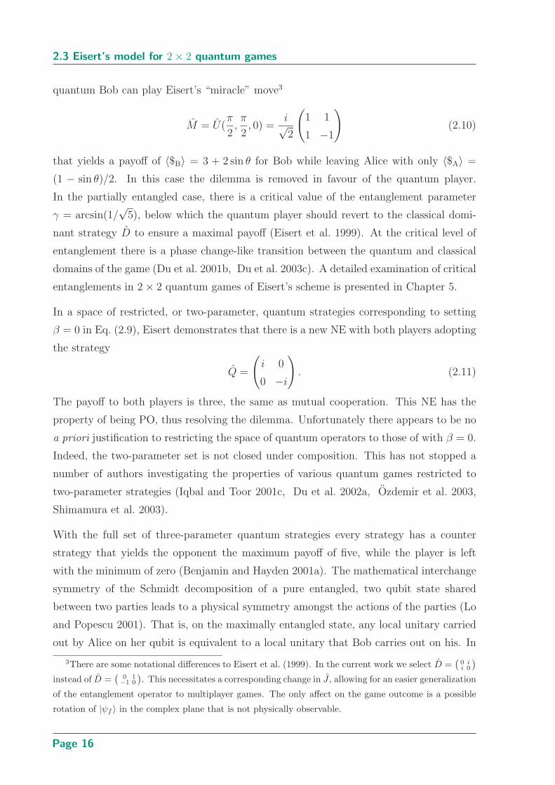
quantum Bob can play Eisert’s “miracle” move3
M = U(π
2,π
2, 0) =
i√2
(
1 1
1 −1
)
(2.10)
that yields a payoff of 〈$B〉 = 3 + 2 sin θ for Bob while leaving Alice with only 〈$A〉 =
(1 − sin θ)/2. In this case the dilemma is removed in favour of the quantum player.
In the partially entangled case, there is a critical value of the entanglement parameter
γ = arcsin(1/√
5), below which the quantum player should revert to the classical domi-
nant strategy D to ensure a maximal payoff (Eisert et al. 1999). At the critical level of
entanglement there is a phase change-like transition between the quantum and classical
domains of the game (Du et al. 2001b, Du et al. 2003c). A detailed examination of critical
entanglements in 2 × 2 quantum games of Eisert’s scheme is presented in Chapter 5.
In a space of restricted, or two-parameter, quantum strategies corresponding to setting
β = 0 in Eq. (2.9), Eisert demonstrates that there is a new NE with both players adopting
the strategy
Q =
(
i 0
0 −i
)
. (2.11)
The payoff to both players is three, the same as mutual cooperation. This NE has the
property of being PO, thus resolving the dilemma. Unfortunately there appears to be no
a priori justification to restricting the space of quantum operators to those of with β = 0.
Indeed, the two-parameter set is not closed under composition. This has not stopped a
number of authors investigating the properties of various quantum games restricted to
two-parameter strategies (Iqbal and Toor 2001c, Du et al. 2002a, Ozdemir et al. 2003,
Shimamura et al. 2003).
With the full set of three-parameter quantum strategies every strategy has a counter
strategy that yields the opponent the maximum payoff of five, while the player is left
with the minimum of zero (Benjamin and Hayden 2001a). The mathematical interchange
symmetry of the Schmidt decomposition of a pure entangled, two qubit state shared
between two parties leads to a physical symmetry amongst the actions of the parties (Lo
and Popescu 2001). That is, on the maximally entangled state, any local unitary carried
out by Alice on her qubit is equivalent to a local unitary that Bob carries out on his. In
3There are some notational differences to Eisert et al. (1999). In the current work we select D =(
0 ii 0
)
instead of D =(
0 1−1 0
). This necessitates a corresponding change in J , allowing for an easier generalization
of the entanglement operator to multiplayer games. The only affect on the game outcome is a possible
rotation of |ψf 〉 in the complex plane that is not physically observable.
Page 16
Chapter 2 Introduction to Quantum Games
terms of our notation, ∀ A = U(θ, α, β) ∃ B = U(θ, α,−π2− β) such that
(A ⊗ I)1√2(|00〉 + i|11〉) = (I ⊗ B)
1√2(|00〉 + i|11〉). (2.12)
So for any strategy U(θ, α, β) chosen by Alice, Bob has the counter DU(θ,−α, π2− β),
essentially “undoing” Alice’s move and then defecting. Hence there is no equilibrium in
pure quantum strategies.
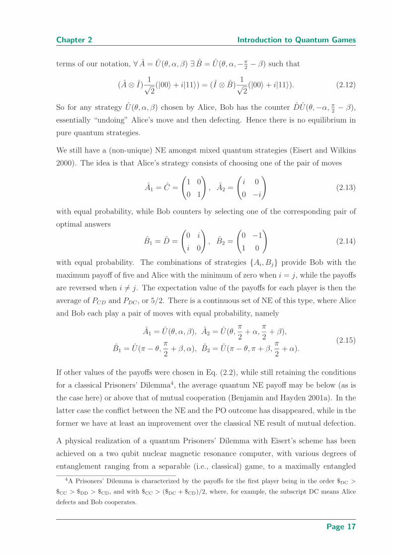
We still have a (non-unique) NE amongst mixed quantum strategies (Eisert and Wilkins
2000). The idea is that Alice’s strategy consists of choosing one of the pair of moves
A1 = C =
(
1 0
0 1
)
, A2 =
(
i 0
0 −i
)
(2.13)
with equal probability, while Bob counters by selecting one of the corresponding pair of
optimal answers
B1 = D =
(
0 i
i 0
)
, B2 =
(
0 −1
1 0
)
(2.14)
with equal probability. The combinations of strategies Ai, Bj provide Bob with the
maximum payoff of five and Alice with the minimum of zero when i = j, while the payoffs
are reversed when i 6= j. The expectation value of the payoffs for each player is then the
average of PCD and PDC , or 5/2. There is a continuous set of NE of this type, where Alice
and Bob each play a pair of moves with equal probability, namely
A1 = U(θ, α, β), A2 = U(θ,π
2+ α,
π
2+ β),
B1 = U(π − θ,π
2+ β, α), B2 = U(π − θ, π + β,
π
2+ α).
(2.15)
If other values of the payoffs were chosen in Eq. (2.2), while still retaining the conditions
for a classical Prisoners’ Dilemma4, the average quantum NE payoff may be below (as is
the case here) or above that of mutual cooperation (Benjamin and Hayden 2001a). In the
latter case the conflict between the NE and the PO outcome has disappeared, while in the
former we have at least an improvement over the classical NE result of mutual defection.
A physical realization of a quantum Prisoners’ Dilemma with Eisert’s scheme has been
achieved on a two qubit nuclear magnetic resonance computer, with various degrees of
entanglement ranging from a separable (i.e., classical) game, to a maximally entangled
4A Prisoners’ Dilemma is characterized by the payoffs for the first player being in the order $DC >
$CC > $DD > $CD, and with $CC > ($DC + $CD)/2, where, for example, the subscript DC means Alice
defects and Bob cooperates.
Page 17
2.3 Eisert’s model for 2 × 2 quantum games
one (Du et al. 2002b). Good agreement between theory and experiment was obtained.
There is also a proposed implementation of the game on an optical quantum computer
(Zhou and Kuang 2003).
The prescription provided by Eisert et al. is a general one that can be applied to any
2× 2 game. Extensions to larger strategic spaces and additional players are considered in
Sec. 2.4. A possible classification scheme for 2 × 2 games in the Eisert model is given by
Huertas-Rosero (2004). Issues that have been studied in this model include ESS (Iqbal
and Toor 2001c), decoherence (Chen et al. 2003b, Flitney and Abbott 2004a, Flitney
and Abbott 2005), quantum versus classical players (Piotrowski and SÃladowski 2003c,
Flitney and Abbott 2003a, Cheon 2004), and differences between classical and quantum
correlations (Ozdemir et al. 2003, Shimamura et al. 2003).
A related protocol is that of Marinatto and Weber (2000). Their scheme differs from
Eisert’s in the omission of the J† gate and by restricting the players’ strategies to proba-
bilistic mixtures of the identity and bit-flip operations. Their scheme effectively chooses
an initial state of (|00〉 + |11〉)/√
2, upon which the players act with a mixture of I and
σx. The classical game is reproduced when the initial state is chosen to be |00〉. Other
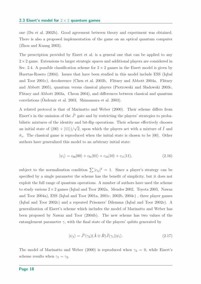
authors have generalized this model to an arbitrary initial state:
|ψi〉 = c00|00〉 + c01|01〉 + c10|10〉 + c11|11〉, (2.16)
subject to the normalization condition∑ |cij|2 = 1. Since a player’s strategy can be
specified by a single parameter the scheme has the benefit of simplicity, but it does not
exploit the full range of quantum operations. A number of authors have used the scheme
to study various 2× 2 games (Iqbal and Toor 2002a, Mendes 2002, Toyota 2003, Nawaz
and Toor 2004a), ESS (Iqbal and Toor 2001a, 2001c, 2002b, 2004c) , three player games
(Iqbal and Toor 2002c) and a repeated Prisoners’ Dilemma (Iqbal and Toor 2002e). A
generalization of Eisert’s scheme which includes the model of Marinatto and Weber has
been proposed by Nawaz and Toor (2004b). The new scheme has two values of the
entanglement parameter γ, with the final state of the players’ qubits generated by
|ψf〉 = J†(γ2)(A ⊗ B)J(γ1)|ψi〉. (2.17)
The model of Marinatto and Weber (2000) is reproduced when γ2 = 0, while Eisert’s
scheme results when γ1 = γ2.
Page 18

Chapter 2 Introduction to Quantum Games
|0〉
|0〉
|0〉
⊗
|ψf〉
J J†U1
U2
UN
......
-time
Figure 2.3. Protocol for an N-person quantum game. A protocol for an N -person quantum
game, where Uj is the move of the jth player and J is an entangling gate (Benjamin
and Hayden 2001b).
2.4 Larger strategic spaces
The field of quantum games has been extended to multiplayer games and games with more
than two classical strategies. As situations become more complex there is more flexibility
in the method of quantization. Additional players are easily accommodated in Eisert’s
protocol by the addition of qubits to the initial state and of extra player operators, as first
discussed by Benjamin and Hayden (2001b) in a scheme inspired by N. F. Johnson. The
scheme is shown in Figure 2.3. The entanglement operator of Eq. (2.7) creates maximal
entanglement between the players’ qubits.
Several authors have examined three and four player quantum games (Benjamin and
Hayden 2001b, Kay et al. 2001, Du et al. 2002a, Du et al. 2002d, Han et al. 2002b).
These offer a greater richness of equilibria than two player games. For example, it is
possible to construct a Prisoners’ Dilemma-like three handed game that has a NE in pure
quantum strategies that is either better or worse than the classical one (Benjamin and
Hayden 2001b).
A game where entanglement can be exploited particularly effectively is the multiplayer
Minority game. The players have the choice of selecting either zero or one. If they
select the least popular choice they are rewarded. No reward is given if the numbers are
balanced. Classically the players can do no better than making a random selection, and
the situation is not improved in the three player quantum version. In the four player
classical game half the time there is no minority, so each player wins on average only
one time in eight. However, entanglement in the quantum version allows us to avoid this
Page 19

2.5 Other models
outcome and provides a NE which rewards each player with probability one quarter, twice
the classical average (Benjamin and Hayden 2001b).
A way of implementing multiplayer games with only two particle entanglement has been
suggested by Chen et al. (2002). In this model, each pair of players, or just neighbouring
players, share a maximally entangled pair of qubits.
The appearance of cooperation in multiplayer games is a feature of classical game theory.
Attempts have been made to consider this in the quantum realm (Iqbal and Toor 2002c,
Ma et al. 2002).
Games with more than two classical strategies can be modeled by replacing the qubits
representing the players’ decisions by an n-state quantum system (or qunit) for the n-
choice case. The space of unitary quantum strategies is expanded from SU(2) to SU(n).
The childhood game of rock-scissors-paper, where the players have three choices, has been
examined by Iqbal and Toor (2002d). However, to make the game amenable to analysis,
the authors do not allow the players the full range of unitary operations, but rather restrict
the strategies to mixtures of I and two operators that involve the interchange of a pair of
states. Entanglement still provides for an enrichment over the classical game.
Another three-strategy game that has been examined is the Monty Hall problem, the
subject of Chapter 3. There are three distinct quantizations in the literature (Li et al.
2001, Flitney and Abbott 2002c, D’Ariano et al. 2002). Chen et al. (2003a) consider
n1 × n2 quantum games with a restricted strategic space akin to a generalization of the
scheme of Marinatto and Weber (2000) to multiple strategies.
2.5 Other models
Apart from the ideas considered above, there have been a variety of other quantum game-
theoretic investigations. These include games that do not involve entanglement (Du et al.
2002c, Grib and Parfionov 2002, Liu and Sun 2002), games of incomplete information
(Han et al. 2002a), continuous variable quantum games (Li et al. 2002), and a game that
involves EPR-type correlated spins (Iqbal 2004, Iqbal and Weigert 2004) that departs
from the models most commonly considered in the literature. A new representation of
game theory that encompasses both classical and quantum games (Wu 2004b) has been
used to create new quantum versions of the Battle of the Sexes (Wu 2004a) and Prisoners’
Dilemma (Wu 2004c).
Page 20

Chapter 2 Introduction to Quantum Games
Some of the mathematical methods of physics have attracted the attention of economists
and a new branch of economic mathematics has appeared, known as econophysics. Polish
theorists Piotrowski and SÃladkowski have proposed a quantum-like approach to economics
with its roots in quantum game theory (Piotrowski 2003, Piotrowski and SÃladkowski
2001, 2002a, 2002b, 2002c, 2002d, 2002e, 2003b, 2003c, 2004b, SÃladkowski 2003). This,
of course, must be distinguished from attempts to use the mathematical machinery of
quantum field theory to solve classical financial market problems (Ilinski 2001, Baaquie
2001, Bonnet et al. 2004). In the new quantum market games, transactions are described
in terms of projective operations acting on Hilbert spaces of strategies of traders. A quan-
tum strategy represents a superposition of trading actions and can achieve outcomes not
realizable by classical means (Piotrowski and SÃladowski 2002d). Furthermore, quantum
mechanics has features that can be used to model aspects of market behavior. For exam-
ple, traders observe the actions of other players and adjust their actions accordingly, so
there is non-commutativity of bidding (Piotrowski and SÃladowski 2001), maximal capital
flow at a given price corresponds to entanglement between buyers and sellers (Piotrowski
and SÃladowski 2002e), and so on.
Parrondo’s paradox, or Parrondo’s games, arise when two games that are losing when
played in isolation can be played in a combination to form an overall winning game
(Harmer and Abbott 1999a, Harmer and Abbott 1999b). There has been much interest
in creating quantum versions of Parrondo’s games (Meyer 2002, Flitney et al. 2002,
Flitney and Abbott 2003c, Ng and Abbott 2004), along with the suggestion that they
can possibly be utilized to increase efficiency of quantum algorithms (Lee et al. 2002, Lee
and Johnson 2002a). Quantum Parrondo’s games are the subject of Chapter 7.
There has been some criticism of quantum games with claims that both Meyer’s quantum
Penny Flip and Eisert’s quantum Prisoners’ Dilemma are not truly quantum mechanical
(van Enk 2000, van Enk and Pike 2002). In the first case, it is true that the strategy
of the quantum player can be implemented classically, however, any classical implemen-
tation would scale exponentially with an increase in the size of the Hilbert space, unlike
a quantum implementation (Meyer 2000). In the case of the two-parameter quantum
Prisoners’ Dilemma, van Enk and Pike (2002) consider this equivalent to a new classical
game with three strategies C, D and Q, and as a result the Q, Q NE does not address
the dilemma in the original game. In addition, the sharing of an entangled state blurs the
distinction between cooperative and non-cooperative games. While these criticisms have
some merit, there is still the issue of efficient implementation of the game and they miss
Page 21
2.6 Summary
the main reason for studying quantum games, which is not as another model for classical
game situations but as a model for competitive scenarios involving quantum information
or quantum control.
2.6 Summary
Game theory is the mathematical theory of decision making in competitive situations.
The new field of quantum game theory is the extension of game theory into the quantum
realm. A protocol for two player, two strategy quantum games has been discussed with
indications of how this can be extended to more players and larger strategic spaces.
Examples of the various quantum game-theoretic investigations in the literature have
been given. In general, the quantum representation of a classical game is not unique, but
all contain the original classical game as a subset. The full set of quantum operations can
be represented by trace-preserving, completely-positive maps. The possibilities where
those operations are not unitary, such as the use of ancillas and the performance of
measurements, remain little explored.
Quantization of a game can lead to either the appearance or disappearance of Nash
equilibria. The much enhanced strategic space available to the players makes the quantum
game more efficient than its classical counter part (Lee and Johnson 2003a). For example,
the gap between the Pareto optimal outcome and the Nash equilibrium in the Prisoners’
Dilemma is reduced or eliminated, and the average payoff in a multiplayer Minority game
is increased, when players are permitted to use (mixed) quantum strategies. There are no
NE in the space of pure quantum strategies in an entangled, fair, 2 × 2 quantum game.
However, general results for many player or repeated games remain to be discovered.
Although there is some controversy surrounding the exact nature of quantum games, there
is in any case much to learn about the behaviour of the interaction of qubits and quantum
information from quantum game-theoretic models.
Page 22
Chapter 3
Quantum Version of theMonty Hall Problem
THE Monty Hall problem is based around a game show that has
a surprising and counterintuitive optimum strategy. The problem
has a long history in one form or another but only received public
attention in the early 1990s, arousing great passions even amongst faculty
mathematicians many of whom were guilty of the same misunderstandings of
probability theory as the general public! In this chapter the classical Monty
Hall problem is briefly explained. Then we explore how the solution is affected
when quantum probability amplitudes are substituted for classical probabil-
ities and player actions are carried out using quantum operators. Without
entanglement, the quantum version offers nothing that cannot be achieved in
the classical setting using mixed strategies. However, with entanglement one
player can gain an advantage by having access to quantum strategies when
the other does not. When both players can utilize quantum strategies there
is no equilibrium in pure strategies but there is a NE in mixed strategies that
gives the same average payoff as the classical game.
The version presented here is one of three distinct quantum versions of the
problem to appear in the literature.
Page 23
3.1 The Monty Hall problem
Prize behind door 1 2 3 1 2 3
Alice opens door 2 or 3 3 2 2 or 3 3 2
Bob’s initial selection 1 1 1 1 1 1
Bob’s strategy switch do not switch
Bob’s final selection 3 or 2 2 3 1 1 1
Result lose win win win lose lose
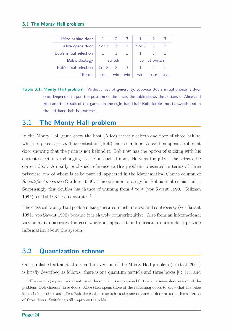
Table 3.1. Monty Hall problem. Without loss of generality, suppose Bob’s initial choice is door
one. Dependent upon the position of the prize, the table shows the actions of Alice and
Bob and the result of the game. In the right hand half Bob decides not to switch and in
the left hand half he switches.
3.1 The Monty Hall problem
In the Monty Hall game show the host (Alice) secretly selects one door of three behind
which to place a prize. The contestant (Bob) chooses a door. Alice then opens a different
door showing that the prize is not behind it. Bob now has the option of sticking with his
current selection or changing to the untouched door. He wins the prize if he selects the
correct door. An early published reference to this problem, presented in terms of three
prisoners, one of whom is to be paroled, appeared in the Mathematical Games column of
Scientific American (Gardner 1959). The optimum strategy for Bob is to alter his choice.
Surprisingly this doubles his chance of winning from 13
to 23
(vos Savant 1990, Gillman
1992), as Table 3.1 demonstrates.5
The classical Monty Hall problem has generated much interest and controversy (vos Savant
1991, vos Savant 1996) because it is sharply counterintuitive. Also from an informational
viewpoint it illustrates the case where an apparent null operation does indeed provide
information about the system.
3.2 Quantization scheme
One published attempt at a quantum version of the Monty Hall problem (Li et al. 2001)
is briefly described as follows: there is one quantum particle and three boxes |0〉, |1〉, and
5The seemingly paradoxical nature of the solution is emphasized further in a seven door variant of the
problem. Bob chooses three doors. Alice then opens three of the remaining doors to show that the prize
is not behind them and offers Bob the choice to switch to the one untouched door or retain his selection
of three doors. Switching still improves the odds!
Page 24
Chapter 3 Quantum Version of the Monty Hall Problem
|2〉. Alice selects a superposition of boxes for her initial placement of the particle and
Bob then selects a particular box. The authors make this a fair game by introducing an
additional particle entangled with the original one and allowing Alice to make a quantum
measurement on this particle as a part of her strategy. If a suitable measurement is taken
after a box is opened it can have the result of changing the state of the original particle
in such a manner as to “redistribute” the particle evenly between the other two boxes. In
the original game Bob has a 23
chance of picking the correct box by altering his choice, but
with this change Bob has 12
probability of being correct by either staying or switching.
A second group quantized the Monty Hall problem with the use of an ancillary system, or
notepad, used by the host (D’Ariano et al. 2002). In this version the position of the prize
is the main quantum variable. It lies in a three-dimensional Hilbert space H, known as
the game space. The position of the prize is prepared quantum mechanically and some
information about this preparation is recorded in the notepad. Bob’s choice of “door” is a
one-dimensional projection p on H. Alice then chooses a one-dimensional projection q and
makes a von Neumann measurement with projections q and I − q, effectively collapsing
the game space to the two-dimensional space (I − q)H. The constraints on q are that it
be orthogonal to p (i.e., a different “door”) and that it does not reveal the position of the
prize. The notepad is used to ensure the latter. Bob can now choose a one-dimensional
projection p′ on (I−q)H and the corresponding measurement on the game space is carried
out to establish whether the prize has been won.
Below, the original Monty Hall problem is quantized directly, without the use of ancillas,
and the host and contestant are both permitted access to quantum strategies. The choices
of Alice and Bob are represented by qutrits6 that are initialized in some state to be
specified later. Their strategies are operators acting on their respective qutrit. A third
qutrit is used to represent the box “opened” by Alice. That is, the the state of the system
can be expressed as
|ψ〉 = |oba〉, (3.1)
where a = Alice’s choice of box, b = Bob’s choice of box, and o = the box that has been
opened. The initial state of the system is designated as |ψi〉. The final state of the system
is
|ψf〉 = B′ O (I ⊗ B ⊗ A)|ψi〉, (3.2)
6A qutrit is the three state generalization of a qubit—a system whose state is a member of a three-
dimensional Hilbert space (Caves and Milburn 2000).
Page 25
3.2 Quantization scheme
where A = Alice’s choice operator, B = Bob’s initial choice operator, O = the opening
box operator, B′ = S (Bob’s switch operator) or N (Bob’s no-switch operator), and I =
the identity operator. Bob can be permitted a mixed strategy on his second move, that is,
selecting S with probability cos2 γ and N with probability sin2 γ, γ ∈ [0, π2]. We shall call
the final state produced when Bob chooses S, |ψSf 〉, and when Bob chooses N , |ψN
f 〉. It
is necessary for the initial state to contain a designation for an open box, but this should
not be taken literally since it does not make sense in the context of the game. The initial
state of the open box is fixed as |0〉.
The open box operator is a unitary operator that can be written
O =∑
ijkℓ
|ǫijk| |njk〉〈ℓjk| +∑
jℓ
|mjj〉〈ℓjj|, (3.3)
where |ǫijk| = 1, if i, j, k are all different and 0 otherwise, m = (j + ℓ + 1) (mod 3),
and n = (i + ℓ) (mod 3). The second term applies to states where Alice would have a
choice of box to open and is one way of providing a unique algorithm for this choice7.
Here and later the summations are over the range 0, 1, 2. We should not consider O to
be the literal action of opening a box and inspecting its contents, which would constitute
a measurement, but rather it is an operator that marks a box by setting the o qutrit in
such a way that it is anti-correlated with Alice’s and Bob’s choices. The coherence of the
system is maintained until the final stage when the payoff is determined by a measurement
on |ψf〉.
Bob’s switch operator can be written as
S =∑
ijkℓ
|ǫijℓ| |iℓk〉〈ijk| +∑
ij
|iij〉〈iij|. (3.4)
The second term is not relevant to the mechanics of the game but is added to ensure
unitarity. Both O and S map each state in the computational basis to a unique basis
state.
N is the identity operator on the three-qutrit state. The A = (aij) and B = (bij) operators
can be selected by the players to operate on their choice of box (that has some initial
value to be specified later) and are restricted to members of SU(3). Bob also selects the
parameter γ that controls the mixture of staying or switching.
7The operator is written this way to ensure unitarity. However, we are only interested in states where
the initial value of the opened box is |0〉, i.e., ℓ = 0. The results for the opened box are inconsistent with
the rules of the game if ℓ = 1 or 2.
Page 26

Chapter 3 Quantum Version of the Monty Hall Problem
It is the expectation value of the payoff that is most important. Bob wins if he picks the
correct box, hence
〈$B〉 = cos2 γ∑
ij
|〈ijj|ψSf 〉|2 + sin2 γ
∑
ij
|〈ijj|ψNf 〉|2 (3.5)
Alice wins if Bob is incorrect, so 〈$A〉 = 1 − 〈$B〉.
3.3 Results
The scheme presented in the previous section is akin to that of Marinatto and Weber
(2000) where there is no entangling operator just a specification of an initial state that
may involve entanglement. The unentangled and maximally entangled initial states are
considered below.
3.3.1 Unentangled initial state
Suppose the initial state of Alice’s and Bob’s choices is an equal mixture of all possible
states with no entanglement:
|ψi〉 = |0〉 ⊗ 1√3(|0〉 + |1〉 + |2〉) ⊗ 1√
3(|0〉 + |1〉 + |2〉). (3.6)
Then
O(I ⊗ B ⊗ A)|ψ〉 =1
3
∑
ijk
|ǫijk| (b0j + b1j + b2j)(a0k + a1k + a2k) |ijk〉
+1
3
∑
j
(b0j + b1j + b2j)(a0j + a1j + a2j) |mjj〉;
SO(I ⊗ B ⊗ A)|ψi〉 =1
3
∑
ijk
|ǫijk| (b0j + b1j + b2j)(a0k + a1k + a2k) |ikk〉
+1
3
∑
jk
|ǫjkm| (b0j + b1j + b2j)(a0j + a1j + a2j) |mkj〉,
(3.7)
where m = (j + 1) (mod 3). This gives
〈$B〉 =1
9cos2 γ
∑
jk
(1 − δjk) |b0j + b1j + b2j|2|a0k + a1k + a2k|2
+1
9sin2 γ
∑
j
|b0j + b1j + b2j|2|a0j + a1j + a2j|2.(3.8)
Page 27
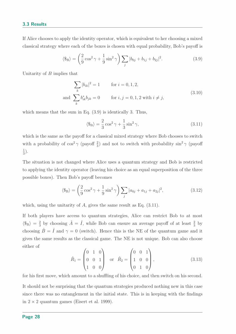
3.3 Results
If Alice chooses to apply the identity operator, which is equivalent to her choosing a mixed
classical strategy where each of the boxes is chosen with equal probability, Bob’s payoff is
〈$B〉 =
(2
9cos2 γ +
1
9sin2 γ
)∑
j
|b0j + b1j + b2j|2. (3.9)
Unitarity of B implies that
∑
k
|bik|2 = 1 for i = 0, 1, 2,
and∑
k
b∗ikbjk = 0 for i, j = 0, 1, 2 with i 6= j,(3.10)
which means that the sum in Eq. (3.9) is identically 3. Thus,
〈$B〉 =2
3cos2 γ +
1
3sin2 γ, (3.11)
which is the same as the payoff for a classical mixed strategy where Bob chooses to switch
with a probability of cos2 γ (payoff 23) and not to switch with probability sin2 γ (payoff
13).
The situation is not changed where Alice uses a quantum strategy and Bob is restricted
to applying the identity operator (leaving his choice as an equal superposition of the three
possible boxes). Then Bob’s payoff becomes
〈$B〉 =
(2
9cos2 γ +
1
9sin2 γ
)∑
j
|a0j + a1j + a2j|2, (3.12)
which, using the unitarity of A, gives the same result as Eq. (3.11).
If both players have access to quantum strategies, Alice can restrict Bob to at most
〈$B〉 = 23
by choosing A = I, while Bob can ensure an average payoff of at least 23
by
choosing B = I and γ = 0 (switch). Hence this is the NE of the quantum game and it
gives the same results as the classical game. The NE is not unique. Bob can also choose
either of
R1 =
0 1 0
0 0 1
1 0 0
or R2 =
0 0 1
1 0 0
0 1 0
, (3.13)
for his first move, which amount to a shuffling of his choice, and then switch on his second.
It should not be surprising that the quantum strategies produced nothing new in this case
since there was no entanglement in the initial state. This is in keeping with the findings
in 2 × 2 quantum games (Eisert et al. 1999).
Page 28

Chapter 3 Quantum Version of the Monty Hall Problem
3.3.2 Maximally entangled initial state
Suppose
|ψi〉 = |0〉 ⊗ 1√3(|00〉 + |11〉 + |22〉), (3.14)
representing maximum entanglement between the choices of Alice and Bob. Now
O(I ⊗ B ⊗ A)|ψi〉 =1√3
∑
ijkℓ
|ǫijk| bℓjaℓk |ijk〉 +1√3
∑
jℓ
bℓjaℓj |mjj〉;
SO(I ⊗ B ⊗ A)|ψi〉 =1√3
∑
ijkℓ
|ǫijk| bℓjaℓk |ikk〉 +1√3
∑
jkℓ
|ǫjkm| bℓjaℓj |mkj〉,(3.15)
where again m = (j + 1) (mod 3). This gives
〈$B〉 =1
3sin2 γ
∑
j
|b0ja0j + b1ja1j + b2ja2j|2
+1
3cos2 γ
∑
jk
(1 − δjk) |b0ja0k + b1ja1k + b2ja2k|2.(3.16)
First consider the case where Bob is limited to a classical mixed strategy. For example,
setting B = I is equivalent to the classical strategy of selecting any of the three boxes
with equal probability. Bob’s payoff is then
〈$B〉 =1
3sin2 γ (|a00|2 + |a11|2 + |a22|2)
+1
3cos2 γ (|a01|2 + |a02|2 + |a10|2 + |a12|2 + |a20|2 + |a21|2).
(3.17)
Alice can then make the game fair by selecting an operator whose diagonal elements all
have an absolute value of 1√2
and whose off-diagonal elements all have absolute value 12.
One such SU(3) operator is
E =
1√2
12
12
−12
3−i√
74√
21+i
√7
4√
2−1−i
√7
4√
2−3+i
√7
85+i
√7
8
. (3.18)
This yields a payoff to both players of 12, whether Bob chooses to switch or not.
The situation where Alice is limited to the identity operator (or any other classical strat-
egy) is uninteresting. Bob can achieve a payoff of 1 by setting B = I and then not
switching. The correlation between Alice’s and Bob’s choice of boxes remains, so Bob is
assured of winning. Bob also wins if he applies R1 or R2 and then switches.
Page 29

3.4 Summary
As noted in Sec. 2.3 every quantum strategy has a counterstrategy. That is, for any
strategy A chosen by Alice, Bob has the counter A∗:
(A∗ ⊗ A)1√3(|00〉 + |11〉 + |22〉) = (I ⊗ A†A)
1√3(|00〉 + |11〉 + |22〉)
=1√3(|00〉 + |11〉 + |22〉).
(3.19)
The correlation between Alice’s and Bob’s choices remains, so Bob can achieve a unit
payoff by not switching.
Similarly for any strategy B chosen by Bob, Alice can ensure a win by countering with
A = B∗ if Bob has chosen γ = 0, while a γ = 1 strategy is defeated by B∗R, where R is
R1 or R2 given in Eq. (3.13). As a result there is no NE amongst pure quantum strategies.
Note that Alice can also play a fair game, irrespective of the value of γ provided she knows
B, by choosing B∗E, giving an expected payoff of 12
to both players. An NE amongst
mixed quantum strategies can still be found. Where both players choose to play I, R1
or R2 with equal probabilities neither player can gain an advantage over the classical
payoffs. If Bob chooses to switch all the time, when he has selected the same operator as
Alice, he loses, but the other two times out of three he wins. Not switching produces the
complementary payoff of 〈$B〉 = 13, so the situation is analogous to the classical game.
3.4 Summary
A quantum version of the interesting game show situation known as the Monty Hall
problem has been presented. Direct comparison of results with the other quantum versions
in the literature are problematic since the models are quite different. The version presented
here is, however, the one most closely resembling the classical version of the problem to
which comparisons have been made. In our model, where both participants have access to
quantum strategies maximal entanglement in the initial state produces the same payoffs
as the classical game for any mixed strategy of switching or not-switching. That is, for
the Nash equilibrium strategy the contestant wins two-thirds of the time by switching. If
the host, Alice, has access to quantum strategies while the contestant, Bob, does not, the
game is fair, since Alice can adopt a strategy with an expected payoff of 12
for each player,
while if Bob has access to quantum strategies and Alice does not he can win all the time.
Without entanglement the quantum game confirms our expectations by offering nothing
more than can be achieved using a mixed strategy in a classical setting.
Page 30

Chapter 4
Quantum Truel
IN game theory, a popular model of a struggle for survival among
three competing agents is a truel, a three person generalization of a
duel. Truels contain many interesting game-theoretic problems. In
this chapter a quantum scheme for duels and truels is presented. In the clas-
sical case, the outcome is sensitive to the precise rules under which the truel
is performed and is often counterintuitive. These aspects carry over into our
quantum scheme, but interference amongst the players’ strategies can arise
leading to game equilibria different from the classical case. Extension of the
model to the N -player case and to truels with decoherence are discussed.
Page 31

4.1 Introduction
4.1 Introduction
A situation where there are three competing agents each trying to eliminate the others
is described in game-theoretic terms by a truel. Such situations can arise, for example,
in biology where there are three species competing for limited resources, or in economics
where three companies are competing in a single market place. In the classic wild Western
duel, two gunfighters shoot it out and the winner is the one left standing. This situation
presents few game theoretic difficulties for the participants: shoot first and calculate
the odds later is always the best strategy! When the scenario is generalized to three
or more players the situation is more complex and an intelligent use of strategy can be
beneficial. For example, consider the case where Alice, Bob and Charles decide to settle
their differences with a sequential shoot out, firing in alphabetic order. Suppose Alice has
a one-third chance of hitting, Bob two-thirds, and Charles never misses (see Figure 4.1).
It would seem clear that each player should target the opponent they would least like to
face in a one on one duel. A superficial examination would suggest that missing a turn
by firing in the air would serve no purpose.
Indeed, Bob and Charles are advised to both target their most dangerous opponent:
each other. Clearly Alice does not want to hit Bob with her first shot since then she is
automatically eliminated by Charles. Surprisingly, Alice is better off abstaining (or firing
in the air) in the first round. She then gets the first shot in the resulting duel, a fact
that compensates for her poorer marksmanship. Precise results for this case are given
below. The paradox of not wanting to fire can been seen most clearly when all three
protagonists are perfect shots. Alice is advised not to shoot since after she eliminates
one of the others she automatically becomes the target for the third. Unless this is the
last round, Bob prefers not to fire as well for the same reason. If there is an unlimited
number of rounds, no one wants to be the first to eliminate an opponent. The result is a
paradoxical stalemate where all survive.
4.2 The classical truel
In the literature various rules for truels are explored. Firing can be simultaneous or
sequential in a fixed or random order, firing into the air can be permitted or not, and the
amount of ammunition can be fixed or unlimited. In the current discussion the following
assumptions are made:
Page 32

Chapter 4 Quantum Truel
Figure 4.1. Schematic of a truel. A truel between Alice, Bob and Charles. In the game Alice can
shoot first, then Bob and then Charles. The firing continues clockwise until only one
player survives. The probability of a hit is shown beneath the player names.
• Each player strictly prefers survival over non-survival. Without loss of generality
we assign a utility of one to a sole survivor and zero to any eliminated players.
• Each player prefers survival with the fewest co-players. That is, the utility of survival
in a pair (u2) or in a three-some (u3) will satisfy the relation 0 < u3 ≤ u2 ≤ 1.
• Alice, Bob and Charles have marksmanship (probability of hitting their chosen
target) of a = 1 − a, b = 1 − b, c = 1 − c, respectively, independent of their target
and with 0 ≤ a, b, c < 1. There is no probability of hitting a person other than the
one chosen.
• The players get no information on the others’ strategies apart from knowing who
has been hit, and in the quantum model not even that.
• Players fire sequentially in alphabetic order with firing into the air permitted.
An analysis of classical truels is provided by Kilgour for the simultaneous (Kilgour 1972).
and the sequential case (Kilgour 1975) A non technical discussion is provided by Kilgour
and Brams (1997). To get a flavour of some of Kilgour’s results we shall consider the
case where the poorest shot fires first and the best last (a < b < c) and ammunition is
unlimited. First, the expectation value of Alice’s payoff in a duel between Alice and Bob,
with each having m bullets, is calculated (see Figure 4.2):
〈$A〉m = 1 − a + ab 〈$A〉m−1. (4.1)
When m → ∞, 〈$A〉m = 〈$A〉m−1, hence
〈$A〉∞ =1 − a
1 − ab. (4.2)
Page 33
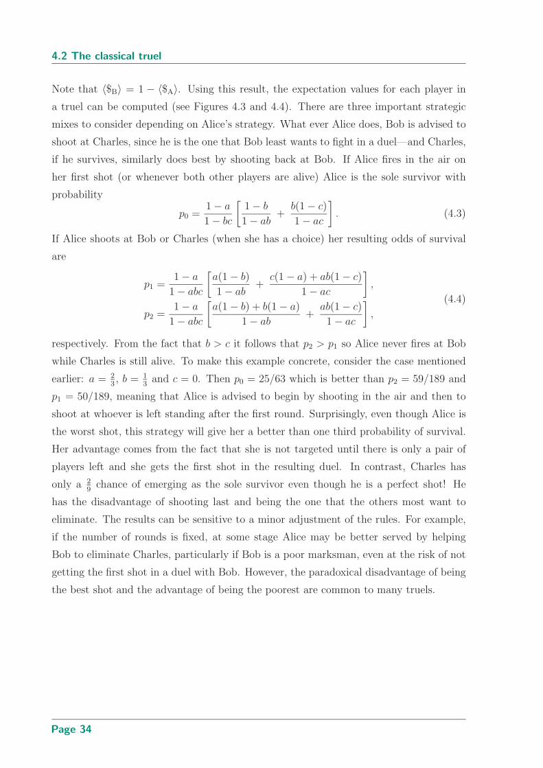
4.2 The classical truel
Note that 〈$B〉 = 1 − 〈$A〉. Using this result, the expectation values for each player in
a truel can be computed (see Figures 4.3 and 4.4). There are three important strategic
mixes to consider depending on Alice’s strategy. What ever Alice does, Bob is advised to
shoot at Charles, since he is the one that Bob least wants to fight in a duel—and Charles,
if he survives, similarly does best by shooting back at Bob. If Alice fires in the air on
her first shot (or whenever both other players are alive) Alice is the sole survivor with
probability
p0 =1 − a
1 − bc
[1 − b
1 − ab+
b(1 − c)
1 − ac
]
. (4.3)
If Alice shoots at Bob or Charles (when she has a choice) her resulting odds of survival
are
p1 =1 − a
1 − abc
[a(1 − b)
1 − ab+
c(1 − a) + ab(1 − c)
1 − ac
]
,
p2 =1 − a
1 − abc
[a(1 − b) + b(1 − a)
1 − ab+
ab(1 − c)
1 − ac
]
,
(4.4)
respectively. From the fact that b > c it follows that p2 > p1 so Alice never fires at Bob
while Charles is still alive. To make this example concrete, consider the case mentioned
earlier: a = 23, b = 1
3and c = 0. Then p0 = 25/63 which is better than p2 = 59/189 and
p1 = 50/189, meaning that Alice is advised to begin by shooting in the air and then to
shoot at whoever is left standing after the first round. Surprisingly, even though Alice is
the worst shot, this strategy will give her a better than one third probability of survival.
Her advantage comes from the fact that she is not targeted until there is only a pair of
players left and she gets the first shot in the resulting duel. In contrast, Charles has
only a 29
chance of emerging as the sole survivor even though he is a perfect shot! He
has the disadvantage of shooting last and being the one that the others most want to
eliminate. The results can be sensitive to a minor adjustment of the rules. For example,
if the number of rounds is fixed, at some stage Alice may be better served by helping
Bob to eliminate Charles, particularly if Bob is a poor marksman, even at the risk of not
getting the first shot in a duel with Bob. However, the paradoxical disadvantage of being
the best shot and the advantage of being the poorest are common to many truels.
Page 34
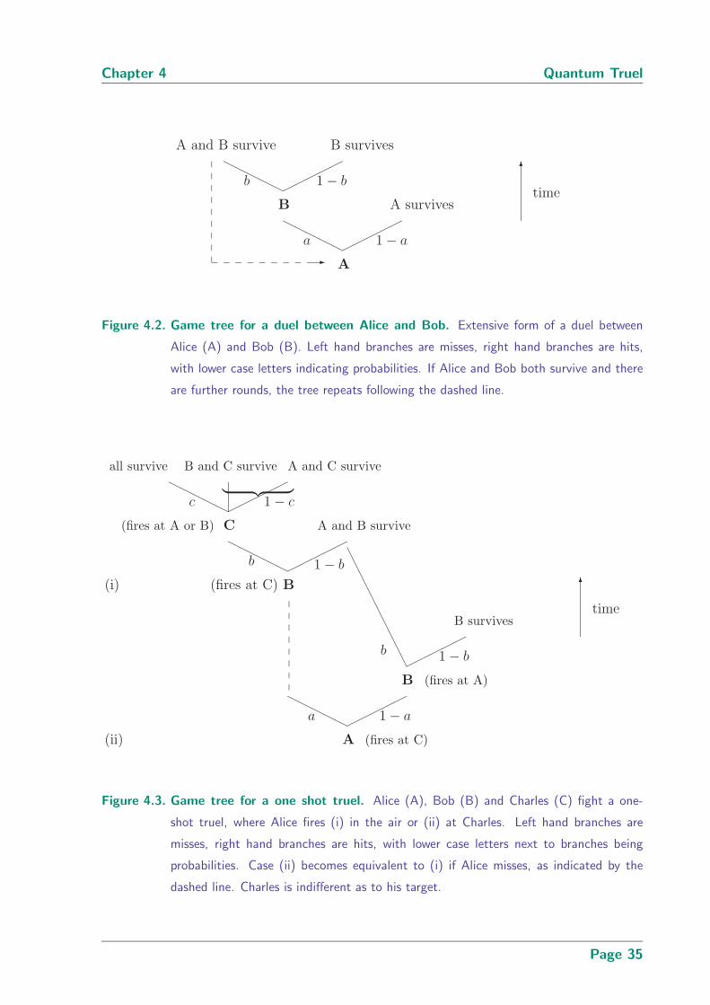
Chapter 4 Quantum Truel
A
HHHHH
©©©©©
B A survives
HHHHH
©©©©©
A and B survive B survives
a 1 − a
b 1 − b
-
6
time
Figure 4.2. Game tree for a duel between Alice and Bob. Extensive form of a duel between
Alice (A) and Bob (B). Left hand branches are misses, right hand branches are hits,
with lower case letters indicating probabilities. If Alice and Bob both survive and there
are further rounds, the tree repeats following the dashed line.
A (fires at C)
HHHHH
©©©©©
B (fires at A)
©©©©©AA
AA
AA
AA
AA
B survives
a 1 − a
b 1 − b
B(fires at C)
HHHHH
©©©©©
C(fires at A or B) A and B survive
HHHHH
©©©©©
all survive B and C survive A and C survive
b 1 − b
c 1 − c︸ ︷︷ ︸
(i)
(ii)
6
time
Figure 4.3. Game tree for a one shot truel. Alice (A), Bob (B) and Charles (C) fight a one-
shot truel, where Alice fires (i) in the air or (ii) at Charles. Left hand branches are
misses, right hand branches are hits, with lower case letters next to branches being
probabilities. Case (ii) becomes equivalent to (i) if Alice misses, as indicated by the
dashed line. Charles is indifferent as to his target.
Page 35

4.3 Quantization scheme
A (fires at C)
HHHHH
©©©©©
B (fires at A)
©©©©©AA
AA
AA
AA
AA
B survives
a 1 − a
b 1 − b
B(fires at C)
HHHHH
©©©©©
C(fires at B) one shot duel between A and B
HHHHH
©©©©©
one shot truel one shot duel between A and C
b 1 − b
c 1 − c
(iii)
(iv)
6
time
Figure 4.4. Game tree for a two-shot truel. Alice (A), Bob (B) and Charles (C) fight a two-shot
truel, where Alice initially fires (iii) in the air or (iv) at Charles. Left hand branches are
misses, right hand are hits, with lower case letters next to branches being probabilities.
Case (iv) becomes equivalent to (iii) if Alice misses her first shot, as indicated. For a
truel of m > 2 shots, the one shot duels become m − 1 shot duels, and the one shot
truel becomes an m − 1 shot truel, with the tree being entered again from the base.
4.3 Quantization scheme
Although the Eisert protocol has become the standard in the literature for 2×2 quantum
games, the quantization of more complex situations is less well established and is certainly
not unique8. The following model of a quantum truel is presented. Each player has a
qubit designating their state, with the computational basis states |0〉 and |1〉 representing
“dead” and “alive,” respectively. The combined state of the players is
|ψ〉 = |qA〉 ⊗ |qB〉 ⊗ |qC〉 = |qA qB qC〉, (4.5)
with the initial state being |ψi〉 = |111〉. In a quantum duel the third qubit is omitted. In a
classical truel the players are located separately, however, in the quantum case the qubits
8For example, in Chapter 3 the case of the Monty Hall problem was discussed, for which there are
three distinct quantum versions in the literature (Li et al. 2001, D’Ariano et al. 2002, Flitney and
Abbott 2002c).
Page 36

Chapter 4 Quantum Truel
representing the states of the players need to be in the one location so that operations
can be carried out on the combined state. We envisage, for example, a referee applying
operators to |ψ〉 with the prior instruction of the players. The analogue of firing at an
opponent is an attempt to flip an opponent’s qubit using a unitary operator acting on |ψ〉.In a duel between Alice and Bob, the action of Alice “firing” at Bob with a probability of
success of a = sin2(θ/2) can be represented, with maximum generality, by the operator
AB =[e−iα cos(θ/2)|11〉 + ieiβ sin(θ/2)|10〉
]〈11|
+[eiα cos(θ/2)|10〉 + ie−iβ sin(θ/2)|11〉
]〈10|
+ |00〉〈00| + |01〉〈01|,
(4.6)
where θ ∈ [0, π] determines the marksmanship and α, β ∈ [−π, π] are arbitrary phase
factors. The last two terms of Eq. (4.6) result from the fact that Alice can do nothing
if her qubit is in the |0〉 state. The operator for Bob “firing” at Alice, BA, is obtained
by reversing the roles of the first and second qubits in Eq. (4.6). For a truel, similar
expressions can be obtained with the third qubit being a spectator. For example,
AB =∑
j
[e−iα cos(θ/2)|11j〉 + ieiβ sin(θ/2)|10j〉
]〈11j|
+[eiα cos(θ/2)|10j〉 + ie−iβ sin(θ/2)|11j〉
]〈10j|
+
∑
jk
|0jk〉〈0jk|(4.7)
is the operation of Alice “firing” at Bob. That is, Alice carries out a control-rotation
of Bob’s qubit with her qubit being the control (see Figure 4.5). Firing into the air is
represented by the identity operator. For α, β and θ the subscripts A, B and C shall be
used to refer to Alice, Bob and Charles, respectively. The operators in Eqs. (4.6–4.7) flip
between |0〉 and |1〉 but do not invert a general |ψ〉. A general complementing operation
in quantum mechanics cannot be achieved unitarily (Buzek et al. 1999, Pati 2001, Pati
2002). The truel shall be of a fixed number of rounds with the coherence of the state
being maintained until a measurement is taken on the final state. Partial decoherence at
each step, where the players obtain some information about the state of the system, is a
possible extension of our scheme, to be considered in Sec. 4.7. Expectation values for the
payoffs to Alice, Bob and Charles are, respectively,
〈$A〉 = |〈100|ψf〉|2 + u2( |〈110|ψf〉|2 + |〈101|ψf〉|2) + u3|〈111|ψf〉|2,〈$B〉 = |〈010|ψf〉|2 + u2( |〈110|ψf〉|2 + |〈011|ψf〉|2) + u3|〈111|ψf〉|2,〈$C〉 = |〈001|ψf〉|2 + u2( |〈101|ψf〉|2 + |〈011|ψf〉|2) + u3|〈111|ψf〉|2.
(4.8)
In what follows, we shall take the utility of surviving in a pair to be u2 = 12
and the utility
of surviving in a trio to be u3 = 13, so that the combined payoff of any outcome is one.
Page 37
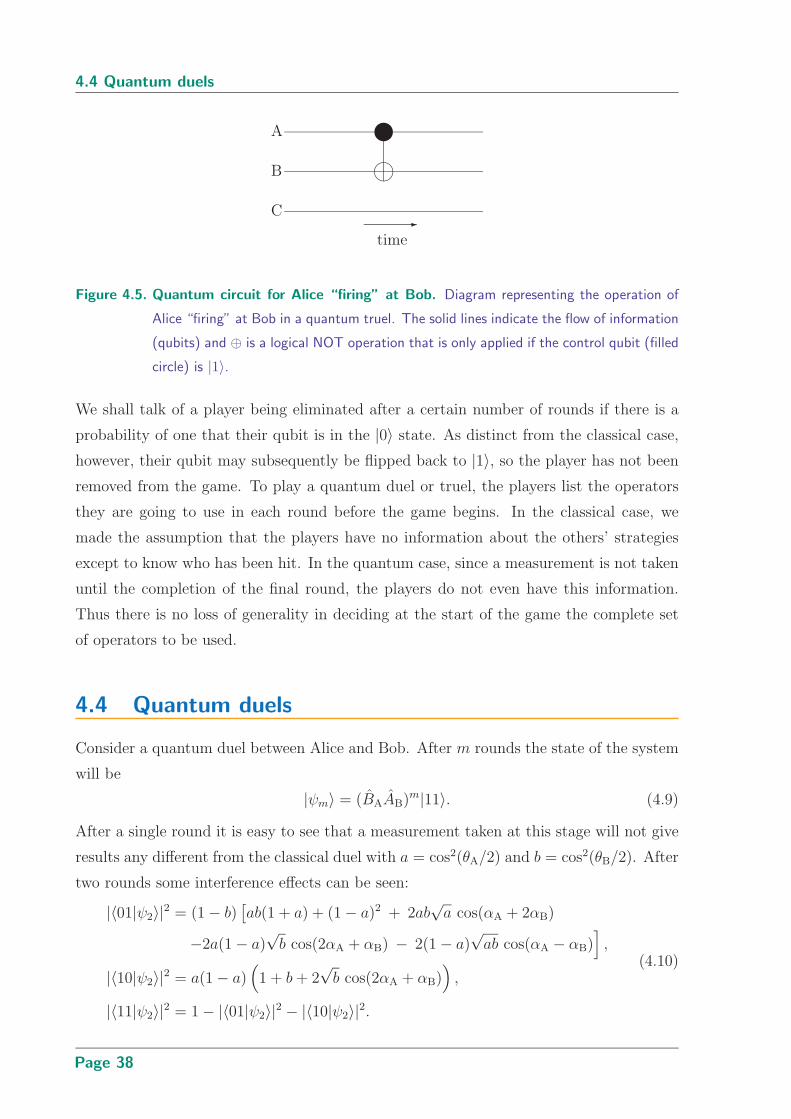
4.4 Quantum duels
A
B
C
m
-
time
Figure 4.5. Quantum circuit for Alice “firing” at Bob. Diagram representing the operation of
Alice “firing” at Bob in a quantum truel. The solid lines indicate the flow of information
(qubits) and ⊕ is a logical NOT operation that is only applied if the control qubit (filled
circle) is |1〉.
We shall talk of a player being eliminated after a certain number of rounds if there is a
probability of one that their qubit is in the |0〉 state. As distinct from the classical case,
however, their qubit may subsequently be flipped back to |1〉, so the player has not been
removed from the game. To play a quantum duel or truel, the players list the operators
they are going to use in each round before the game begins. In the classical case, we
made the assumption that the players have no information about the others’ strategies
except to know who has been hit. In the quantum case, since a measurement is not taken
until the completion of the final round, the players do not even have this information.
Thus there is no loss of generality in deciding at the start of the game the complete set
of operators to be used.
4.4 Quantum duels
Consider a quantum duel between Alice and Bob. After m rounds the state of the system
will be
|ψm〉 = (BAAB)m|11〉. (4.9)
After a single round it is easy to see that a measurement taken at this stage will not give
results any different from the classical duel with a = cos2(θA/2) and b = cos2(θB/2). After
two rounds some interference effects can be seen:
|〈01|ψ2〉|2 = (1 − b)[ab(1 + a) + (1 − a)2 + 2ab
√a cos(αA + 2αB)
−2a(1 − a)√
b cos(2αA + αB) − 2(1 − a)√
ab cos(αA − αB)]
,
|〈10|ψ2〉|2 = a(1 − a)(
1 + b + 2√
b cos(2αA + αB))
,
|〈11|ψ2〉|2 = 1 − |〈01|ψ2〉|2 − |〈10|ψ2〉|2.
(4.10)
Page 38
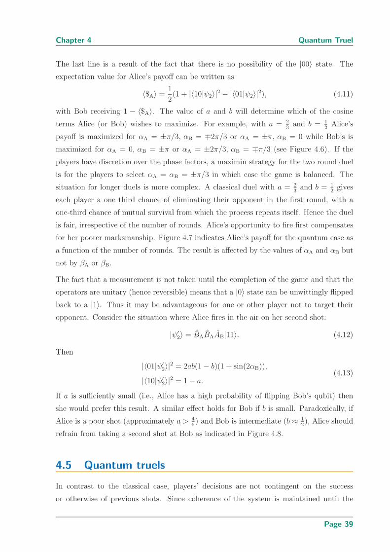
Chapter 4 Quantum Truel
The last line is a result of the fact that there is no possibility of the |00〉 state. The
expectation value for Alice’s payoff can be written as
〈$A〉 =1
2(1 + |〈10|ψ2〉|2 − |〈01|ψ2〉|2), (4.11)
with Bob receiving 1 − 〈$A〉. The value of a and b will determine which of the cosine
terms Alice (or Bob) wishes to maximize. For example, with a = 23
and b = 12
Alice’s
payoff is maximized for αA = ±π/3, αB = ∓2π/3 or αA = ±π, αB = 0 while Bob’s is
maximized for αA = 0, αB = ±π or αA = ±2π/3, αB = ∓π/3 (see Figure 4.6). If the
players have discretion over the phase factors, a maximin strategy for the two round duel
is for the players to select αA = αB = ±π/3 in which case the game is balanced. The
situation for longer duels is more complex. A classical duel with a = 23
and b = 12
gives
each player a one third chance of eliminating their opponent in the first round, with a
one-third chance of mutual survival from which the process repeats itself. Hence the duel
is fair, irrespective of the number of rounds. Alice’s opportunity to fire first compensates
for her poorer marksmanship. Figure 4.7 indicates Alice’s payoff for the quantum case as
a function of the number of rounds. The result is affected by the values of αA and αB but
not by βA or βB.
The fact that a measurement is not taken until the completion of the game and that the
operators are unitary (hence reversible) means that a |0〉 state can be unwittingly flipped
back to a |1〉. Thus it may be advantageous for one or other player not to target their
opponent. Consider the situation where Alice fires in the air on her second shot:
|ψ′2〉 = BABAAB|11〉. (4.12)
Then
|〈01|ψ′2〉|2 = 2ab(1 − b)(1 + sin(2αB)),
|〈10|ψ′2〉|2 = 1 − a.
(4.13)
If a is sufficiently small (i.e., Alice has a high probability of flipping Bob’s qubit) then
she would prefer this result. A similar effect holds for Bob if b is small. Paradoxically, if
Alice is a poor shot (approximately a > 45) and Bob is intermediate (b ≈ 1
2), Alice should
refrain from taking a second shot at Bob as indicated in Figure 4.8.
4.5 Quantum truels
In contrast to the classical case, players’ decisions are not contingent on the success
or otherwise of previous shots. Since coherence of the system is maintained until the
Page 39
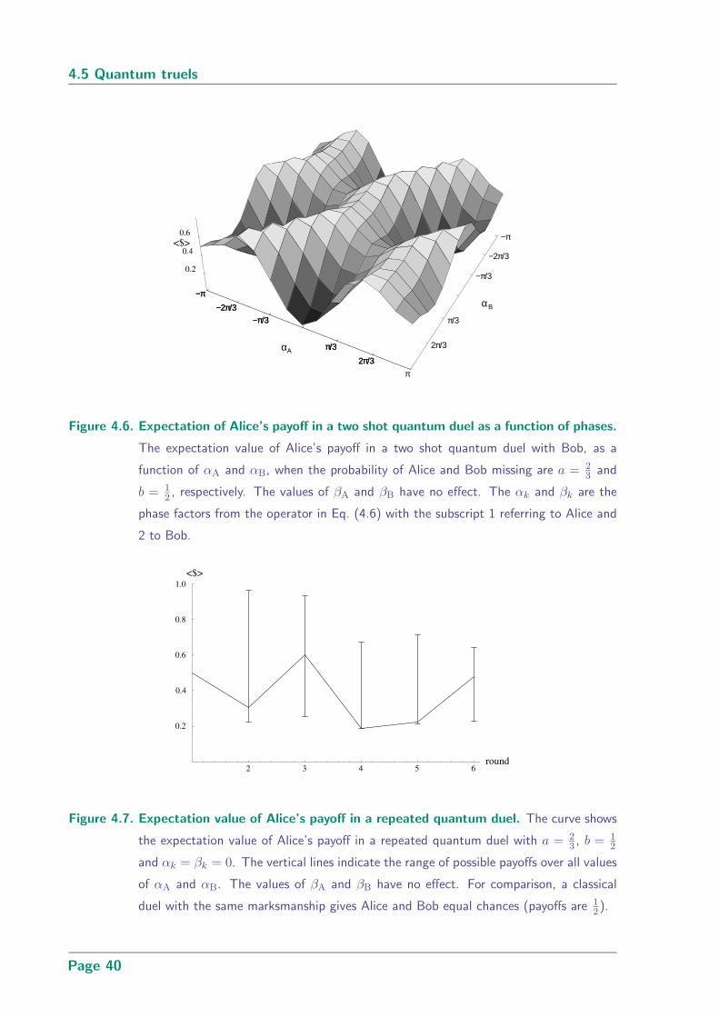
4.5 Quantum truels
−π
−2π/3−π/3
π/3
2π/3π
αΑ2π/3
π/3
−π/3
−2π/3
−π
αΒ
0.2
0.4
0.6
<$>
−π
−2π/3−π/3
π/3
2π/3π
Figure 4.6. Expectation of Alice’s payoff in a two shot quantum duel as a function of phases.
The expectation value of Alice’s payoff in a two shot quantum duel with Bob, as a
function of αA and αB, when the probability of Alice and Bob missing are a = 23 and
b = 12 , respectively. The values of βA and βB have no effect. The αk and βk are the
phase factors from the operator in Eq. (4.6) with the subscript 1 referring to Alice and
2 to Bob.
2 3 4 5 6round
0.2
0.4
0.6
0.8
1.0
<$>
Figure 4.7. Expectation value of Alice’s payoff in a repeated quantum duel. The curve shows
the expectation value of Alice’s payoff in a repeated quantum duel with a = 23 , b = 1
2
and αk = βk = 0. The vertical lines indicate the range of possible payoffs over all values
of αA and αB. The values of βA and βB have no effect. For comparison, a classical
duel with the same marksmanship gives Alice and Bob equal chances (payoffs are 12).
Page 40
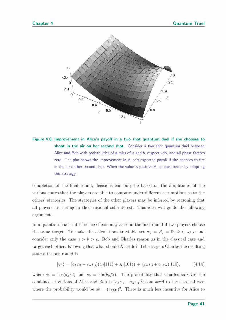
Chapter 4 Quantum Truel
0
0.2
0.4
0.6
0.8
1
a0.8
0.6
0.4
0.2
0
b
-0.5
0
1
<$>
0
0.2
0.4
0.6
0.8
1
Figure 4.8. Improvement in Alice’s payoff in a two shot quantum duel if she chooses to
shoot in the air on her second shot. Consider a two shot quantum duel between
Alice and Bob with probabilities of a miss of a and b, respectively, and all phase factors
zero. The plot shows the improvement in Alice’s expected payoff if she chooses to fire
in the air on her second shot. When the value is positive Alice does better by adopting
this strategy.
completion of the final round, decisions can only be based on the amplitudes of the
various states that the players are able to compute under different assumptions as to the
others’ strategies. The strategies of the other players may be inferred by reasoning that
all players are acting in their rational self-interest. This idea will guide the following
arguments.
In a quantum truel, interference effects may arise in the first round if two players choose
the same target. To make the calculations tractable set αk = βk = 0; k ∈ A,B,C and
consider only the case a > b > c. Bob and Charles reason as in the classical case and
target each other. Knowing this, what should Alice do? If she targets Charles the resulting
state after one round is
|ψ1〉 = (cAcB − sAsB)(cC|111〉 + sC|101〉) + (cAsB + cBsA)|110〉, (4.14)
where ck ≡ cos(θk/2) and sk ≡ sin(θk/2). The probability that Charles survives the
combined attentions of Alice and Bob is (cAcB − sAsB)2, compared to the classical case
where the probability would be ab = (cAcB)2. There is much less incentive for Alice to
Page 41
4.5 Quantum truels
fire in the air since, unlike the classical case, Bob does not change his strategy (to target
Alice) depending on the result of Alice’s operation. If θA and θB are around π/2 then
cAcB ≈ sAsB and both Alice and Bob will like the result of Eq. (4.14) since Charles has
a high probability of being eliminated.
For example, consider the case mentioned in Sec. 4.2 where a = (cA)2 = 23, b = (cB)2 = 1
3
and c = (cC)2 = 0. If both Alice and Bob target Charles, he is eliminated with certainty
in the first round and consequently his strategy is irrelevant! If there are sufficient rounds
Alice would appear to be in difficulty in the resulting two person duel since her marks-
manship is half that of Bob’s. In a repeated quantum duel where both players continue
firing this is indeed the case. However, quantum effects come to her rescue if Alice fires
in the air on her third shot. The expectation value of her payoff after three rounds is
then improved from 0.448 to 0.761. Indeed, Bob’s survival chances are diminished to such
an extent that he is advised to fire in the air on the second and subsequent rounds. We
then reach an equilibrium where it is to the disadvantage of both players to target the
other. Alice emerges with the slightly better prospects (〈$A〉 = 0.554) since she has had
two shots to Bob’s one. As a result of being able to “restore” a player to life (i.e., flip
|0〉 → |1〉) this quantum example is in marked contrast to classical two person duels where
it is never an advantage to fire in the air.
Now, compare this to the option of Alice firing in the air in the first round. With Bob
and Charles targeting each other and Charles being a perfect shot, after the first round
the amplitude of states where both survive is zero. Since Bob fired first and has better
than 50% chance of success, the |110〉 state will have a larger amplitude than the |101〉state, so Alice reasons that it is better for her to target Bob in the second round. Since
only Bob or Charles can have survived the first round they each (if alive) target Alice in
the second.9 After two rounds the resulting state is
|ψ2〉 = (CABAAB)(CBBC)|111〉
=1√27
(−√
6|001〉 −√
8|010〉 −√
6|100〉 − i|011〉 + i√
4|110〉 +√
2|111〉).(4.15)
Before the start of the game Alice calculates that if she survives the first two rounds there
is a 50% chance she is the sole survivor. If she now targets one of the others in the third
round she is more likely to flip a |0〉 state to a |1〉 than the reverse, hence she fires in the
9Recall that coherence of the state is maintained until the completion of the final round, when a
measurement reveals who has been hit. This means that all targeting decisions can be made prior to the
first round.
Page 42

Chapter 4 Quantum Truel
air. The argument for Bob and Charles to do likewise for the same reason is even more
compelling. Hence, even with a large number of rounds, all players choose to fire in the
air after the second round. The resulting payoffs are 〈$A〉 = 52/162, 〈$B〉 = 67/162 and
〈$C〉 = 43/162. Alice clearly prefers to fire at Charles in the first round over this strategy.
It is rare in a quantum truel that Alice will opt to fire in the air in the first round. This is
in contrast to the classical situation where this is often the weakest player’s best strategy.
In situations where one player is not eliminated with certainty, an equilibrium where all
three players prefer to fire in the air will generally arise. Each player reasons that to fire
at an opponent would increase the amplitude of the |1〉 state of their target.
4.5.1 One- and two-shot truel
To clarify some of the differences between the classical and quantum truels, consider the
simple cases of one- and two-shot truels where Charles is a perfect shot. Where Charles
is indifferent as to the choice of target, he uses a fair coin to decide. In the quantum
case, Charles will use this method to select his desired operator before any operations are
carried out on |ψi〉. For tractability, αk = βk = 0 is assumed.
In the one-shot case, Charles is Bob’s only threat so Bob will fire at Charles. Alice may be
targeted by Charles so may wish to help Bob, particularly if he is a poor shot. Because
of interference, this strategy is more likely to be preferred in the quantum case. The
regions of the parameter space (a, b) where Alice should select one strategy over the other
are indicated in Figure 4.9—this figure is of interest because it illustrates a case where
going from a classical to a quantum regime changes a linear boundary in the probability
parameter space into a convex one and such convexity is being intensely studied as it is
the basis of Parrondo’s paradox (Harmer and Abbott 2002).
The situation is more complex in the two-shot case. When a > b, in the first round Bob
and Charles again target each other, while Alice either fires in the air or at Charles. Since
only one of Bob and Charles survive the first round, they both (if alive) target Alice in the
second. In the classical game, Alice’s target in the second round is determined since she
knows whom of Bob or Charles remains. However, in the quantum case this is unknown
and Alice can only base her decision on maximizing the expectation value of her payoff.
The regions of the parameter space (a, b) where Alice prefers the different strategies are
given in Figure 4.10.
Page 43

4.5 Quantum truels
0.2 0.4 0.6 0.8 1.0a
0.2
0.4
0.6
0.8
1.0
bclassical boundary
quantumboundary
Figure 4.9. Alice’s preferred strategy in a one shot quantum truel with Alice being the
poorest shot. In a one-shot truel with c = 0, Alice’s preferred strategy depending on
the values of a and b: Alice fires in the air if (a, b) is below the line (solid line for the
quantum case, dashed line for the classical case) and at Charles, if above. The quantum
boundary is half a parabola whose equation is a = (1 − 2b)2.
If b > a, Charles will target Alice in the first round since she is his most dangerous
opponent. Likewise, Bob targets Charles. In the second round, reasoning as above, both
Alice and Charles (if alive) will target Bob. In the classical case the only strategic choice
is whether Alice fires at Charles or into the air in the first round. In the quantum case
Bob has a decision to make in the second round since he does not know for certain who
was hit in the first. Figure 4.11 shows the regions of parameter space corresponding to
the optimal choices of Alice and Bob.
A classical truel where the players do not know which others have been eliminated may
be a fairer comparison to the quantum situation. This alters the regions corresponding
to the players’ optimal strategies, but there are still differences with the quantum truel
as a result of interference in the latter case.
Page 44

Chapter 4 Quantum Truel
0.2 0.4 0.6 0.8 1.0a
0.2
0.4
0.6
0.8
1.0
b
I I
IIIII
III
IV
Figure 4.10. Alice’s preferred strategy in a two shot quantum truel with Alice being the
poorest shot. The figure shows the parameter space (a, b) divided in into regions
corresponding to Alice’s possible optimal strategies in a two-shot truel with a > b >
c = 0. The optimal strategy also depends on whether the game is classical or quantum.
Classical: I and II, fire into the air and then at the survivor of round one; III and IV,
fire at Charles and then at the survivor of round one. Quantum: I, fire into the air and
then at Bob; II, fire at Charles both times; III, fire at Charles and then at Bob; IV, fire
into the air and then at Charles. The boundary between regions I and III, or II and IV,
is the curved line in the classical case and the dashed line in the quantum case.
4.6 Quantum N-uels
A quantum N -uel can be obtained by adding qubits to the state |ψ〉 in Eq. (4.5):
|ψ〉 = |q1〉 ⊗ |q2〉 ⊗ . . . ⊗ |qN〉, (4.16)
where |qj〉 is the qubit of player j. The players’ operators are the same as Eq. (4.7) except
with additional spectator qubits. For example, the first player firing at the second is
carried out by
AB =∑
j3,...,jN
[e−iα cos(θ/2)|11j3 . . . jN〉 + ieiβ sin(θ/2)|10j3 . . . jN〉
]〈11j3 . . . jN |
+[eiα cos(θ/2)|10j3 . . . jN〉 + ie−iβ sin(θ/2)|11j3 . . . jN〉
]〈10j3 . . . jN |
+∑
j2,...,jN
|0j2 . . . jN〉〈0j2 . . . jN |,
(4.17)
Page 45

4.7 Classical-quantum correspondence
0.2 0.4 0.6 0.8 1.0a
0.2
0.4
0.6
0.8
1.0
b
V
VI
VII
Figure 4.11. Alice and Bob’s preferred strategy in a two shot quantum truel with Bob being
the poorest shot. The figure shows the parameter space (a, b) divided in into regions
corresponding to the possible optimal strategies of Alice and Bob in a two-shot truel
with b > a > c = 0. The optimal strategy also depends on whether the game is
classical or quantum. Classical: in the first round, Alice fires in the air if b < 12 or at
Charles if b > 12 . Quantum: V, Alice fires into the air in round one and Bob fires at
Charles in round two; VI and VII, Alice fires at Charles in round one and Bob fires at
Alice (VI) or Charles (VII) in round two.
where the ji take the values 0 or 1.
The features of the quantum N -uel are the same as those of the quantum truel. Positive
and negative interference arising from multiple players choosing a common target is more
likely and equilibria where it is to the advantage of all (surviving) players to shoot into
the air still arise.
4.7 Classical-quantum correspondence
In the classical case, players are removed from the game once hit. Maintained coherence
through out the quantum game weakens the analogy with classical truel, since players
can be brought back to “life,” that is, have their qubit flipped from |0〉 to |1〉. However,
there is still a correspondence. During the game, a player can only fire if their qubit is
in the |1〉 state, and they receive a zero payoff at the end of the game if their qubit is
Page 46
Chapter 4 Quantum Truel
in the |0〉 state. The classical-quantum correspondence can be enhanced by introducing
partial decoherence after each move and allowing the players to choose their strategy dy-
namically depending on the result of previous rounds. In this case, the classical situation
is reproduced in the limit of full decoherence. If ρ = |ψ〉〈ψ| is the density operator of the
system in state |ψ〉, one way of effecting partial decoherence is by
ρ → (1 − p)ρ + p diag(ρ), (4.18)
where 0 ≤ p ≤ 1. This is equivalent to measuring the state of the system in the com-
putational basis with probability p. When ρ is diagonal, the next player can select their
target based on the measurement result. Figure 4.12 shows the regions of the parameter
space (a, b) corresponding to Alice’s preferred strategy in a one shot truel when Charles is
a perfect shot (the situation of Figure 4.9). The boundary between Alice maximizing her
expected payoff by firing into the air and targeting Charles depends on the measurement
probability p. There is a smooth transition from the quantum case to the classical one as
p goes from zero to one. Decoherence in quantum games has been considered10 by Chen
et al. (2003b) and Flitney and Abbott (2005). Chapter 6 considers this issue in detail.
4.8 Summary
A protocol for quantum duels, truels and N -uels has been presented. While the analogy
with classical duels is not precise, interesting comparisons can still be made. A one
round quantum duel is equivalent to the classical game, but in longer quantum duels the
appearance of phase terms in the operators can greatly affect the expected payoff to the
players. If players have discretion over the value of their phase factors a maximin choice
can in principle be calculated provided the number of rounds is fixed. If one player has
a restricted choice the other has a large advantage. The unitary nature of the operators
means that the probability of flipping a “dead” state to an “alive” state is the same as that
for the reverse, so it can be advantageous for a player to fire in the air rather than target
the opponent, something that is never true in a classical duel. Indeed, an equilibrium can
be reached where both players forgo targeting their opponent even if there are further
rounds to play.
In a quantum truel, strategies are not contingent on earlier results. The players’ entire
strategy (the list of players to target in different rounds) can be mapped out in advance
10Johnson (2001) and Ozdemir et al. (2004) consider a quantum game with an initial state corrupted
by bit flip errors but do not consider decoherence during the game.
Page 47

4.8 Summary
0.2 0.4 0.6 0.8 1.0a
0.2
0.4
0.6
0.8
1.0
b
p
p
p
p
p
=0
=1/4
=1/2
=3/4
=1
Figure 4.12. Alice’s preferred strategy in a one-shot quantum truel with decoherence. In
a one shot quantum truel with c = 0 and with decoherence, the figure shows the
boundaries for different values of the measurement probability p below which Alice
maximizes her expected payoff by firing into the air and above which by targeting
Charles. There is a smooth transition from the fully quantum case (p = 0) to the
classical one (p = 1).
based on the expected amplitudes of the various states resulting from different strategic
choices by the players. Interference effects arise where one player is targeted by the
other two, and can have dramatic consequences, either enhancing or diminishing the
probability of survival of the targeted player compared to the classical case. As with the
case of quantum duels, equilibria can arise where it is to the disadvantage of each player
to target one of the others. Such equilibria arise only in special cases in a classical truel.
Introducing decoherence in the form of a measurement after each move changes the quan-
tum game. As the measurement probability is increased from zero to one there is a smooth
transition from the fully quantum game to the classical one.
Page 48
Chapter 5
Advantage of a QuantumPlayer Over a Classical
Player
IN the Eisert model of 2× 2 quantum games it is known that a player
with access to the full set of quantum strategies has an advantage over
a player limited to the classical subset. In this chapter we quantify
this advantage as a function of the degree of entanglement of the players’
qubits. Several well known 2×2 games are considered, including the Prisoners’
Dilemma, Chicken and the Battle of the Sexes, giving critical values of the
entanglement parameter above which the quantum player’s advantage becomes
apparent. A list of “miracle” moves, or best moves for the quantum player
against a classical player, is provided for arbitrary 2 × 2 quantum games of
the Eisert model.
Page 49
5.1 Introduction
5.1 Introduction
The games that have generated the most discussion in the literature are those that pose
some sort of dilemma, for example, where there is a conflict between multiple NE or where
the NE, though a compelling response for the rational player, is less than optimal. We
have already seen one such game, the Prisoners’ Dilemma, in Chapter 2. A good non-
technical discussion of various dilemmas in 2 × 2 games is given by Poundstone (1992)
from which the names of the games treated in this chapter have been taken. Most of the
classical games discussed appear in any introductory text on game theory. Table 5.1 gives
payoff matrices for various 2 × 2 games. The payoff for the four possible outcomes are
designated a, b, c and d, with a > b > c > d. Typical values for (a, b, c, d) for each game are
given in the table and these shall be used whenever numerical results are desired. In all
the games apart from the Battle of the Sexes, of the two classical strategies, one is helpful
to the opposing player and is known as cooperation (C), while the other is damaging to
the opposing player and is known as defection (D). In the quantum protocol these moves
are represented by the |0〉 and |1〉 states, respectively.
5.2 Miracle moves
As noted in Chapter 2, in a maximally entangled 2 × 2 quantum game of the Eisert
scheme, any pure quantum strategy U(θ, α, β), that is, a local unitary operation carried
out on the player’s own qubit, is equivalent to a different pure strategy U(θ, α,−π2− β)
carried out by the other player, as was seen in Eq. (2.12). Thus, when both players have
access to the full set of quantum operators, if one player’s strategy U(θ, α, β) is known,
the other player can undo this operation by selecting U(θ, α,−π2−β)−1 = U(θ,−α, π
2−β).
Indeed, by choosing a composite strategy U(θ′, α′, β′) U(θ,−α, π2− β) any desired final
state can be produced. The consequence of this for maximally entangled 2 × 2 quantum
games is that there can be no NE amongst pure quantum strategies (Eisert and Wilkins
2000, Benjamin and Hayden 2001a).
The situation is more interesting when one player, say Alice, is restricted to Scl ≡ U(θ) :
θ ∈ [0, π] while the other, Bob, has access to Sq ≡ U(θ, α, β) : θ ∈ [0, π]; α, β ∈ [−π, π].Games with these strategy restrictions shall be referred to as classical–quantum games.
Strategies in Scl are “classical” in the sense that the player simply executes two classical
moves with fixed probabilities and does not manipulate qubit phase. However, U(θ)
only gives the same results as a classical mixed strategy when both players employ these
Page 50
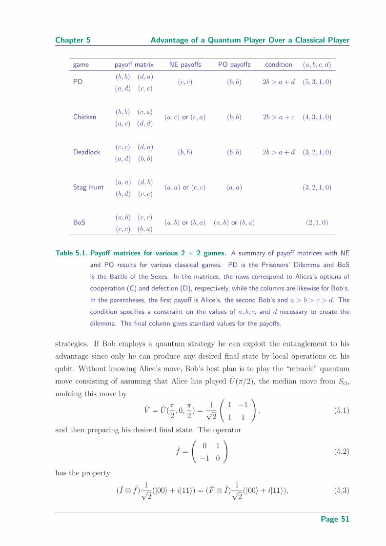
Chapter 5 Advantage of a Quantum Player Over a Classical Player
game payoff matrix NE payoffs PO payoffs condition (a, b, c, d)
PD(b, b) (d, a)
(a, d) (c, c)(c, c) (b, b) 2b > a + d (5, 3, 1, 0)
Chicken(b, b) (c, a)
(a, c) (d, d)(a, c) or (c, a) (b, b) 2b > a + c (4, 3, 1, 0)
Deadlock(c, c) (d, a)
(a, d) (b, b)(b, b) (b, b) 2b > a + d (3, 2, 1, 0)
Stag Hunt(a, a) (d, b)
(b, d) (c, c)(a, a) or (c, c) (a, a) (3, 2, 1, 0)
BoS(a, b) (c, c)
(c, c) (b, a)(a, b) or (b, a) (a, b) or (b, a) (2, 1, 0)
Table 5.1. Payoff matrices for various 2 × 2 games. A summary of payoff matrices with NE
and PO results for various classical games. PD is the Prisoners’ Dilemma and BoS
is the Battle of the Sexes. In the matrices, the rows correspond to Alices’s options of
cooperation (C) and defection (D), respectively, while the columns are likewise for Bob’s.
In the parentheses, the first payoff is Alice’s, the second Bob’s and a > b > c > d. The
condition specifies a constraint on the values of a, b, c, and d necessary to create the
dilemma. The final column gives standard values for the payoffs.
strategies. If Bob employs a quantum strategy he can exploit the entanglement to his
advantage since only he can produce any desired final state by local operations on his
qubit. Without knowing Alice’s move, Bob’s best plan is to play the “miracle” quantum
move consisting of assuming that Alice has played U(π/2), the median move from Scl,
undoing this move by
V = U(π
2, 0,
π
2) =
1√2
(
1 −1
1 1
)
, (5.1)
and then preparing his desired final state. The operator
f =
(
0 1
−1 0
)
(5.2)
has the property
(I ⊗ f)1√2(|00〉 + i|11〉) = (F ⊗ I)
1√2(|00〉 + i|11〉), (5.3)
Page 51
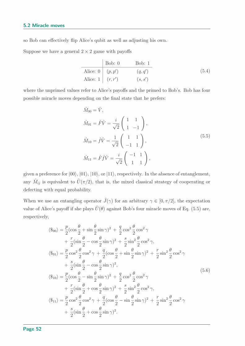
5.2 Miracle moves
so Bob can effectively flip Alice’s qubit as well as adjusting his own.
Suppose we have a general 2 × 2 game with payoffs
Bob: 0 Bob: 1
Alice: 0 (p, p′) (q, q′)
Alice: 1 (r, r′) (s, s′)
(5.4)
where the unprimed values refer to Alice’s payoffs and the primed to Bob’s. Bob has four
possible miracle moves depending on the final state that he prefers:
M00 = V ,
M01 = F V =i√2
(
1 1
1 −1
)
,
M10 = f V =1√2
(
1 1
−1 1
)
,
M11 = F f V =i√2
(
−1 1
1 1
)
,
(5.5)
given a preference for |00〉, |01〉, |10〉, or |11〉, respectively. In the absence of entanglement,
any Mij is equivalent to U(π/2), that is, the mixed classical strategy of cooperating or
defecting with equal probability.
When we use an entangling operator J(γ) for an arbitrary γ ∈ [0, π/2], the expectation
value of Alice’s payoff if she plays U(θ) against Bob’s four miracle moves of Eq. (5.5) are,
respectively,
〈$00〉 =p
2(cos
θ
2+ sin
θ
2sin γ)2 +
q
2cos2 θ
2cos2 γ
+r
2(sin
θ
2− cos
θ
2sin γ)2 +
s
2sin2 θ
2cos2 γ,
〈$01〉 =p
2cos2 θ
2cos2 γ +
q
2(cos
θ
2+ sin
θ
2sin γ)2 +
r
2sin2 θ
2cos2 γ
+s
2(sin
θ
2− cos
θ
2sin γ)2,
〈$10〉 =p
2(cos
θ
2− sin
θ
2sin γ)2 +
q
2cos2 θ
2cos2 γ
+r
2(sin
θ
2+ cos
θ
2sin γ)2 +
s
2sin2 θ
2cos2 γ,
〈$11〉 =p
2cos2 θ
2cos2 γ +
q
2(cos
θ
2− sin
θ
2sin γ)2 +
r
2sin2 θ
2cos2 γ
+s
2(sin
θ
2+ cos
θ
2sin γ)2.
(5.6)
Page 52

Chapter 5 Advantage of a Quantum Player Over a Classical Player
We add primes to p, q, r, and s to get Bob’s payoffs. Although the miracle moves are in
some sense best for Bob, in that they guarantee a certain minimum payoff against any
classical strategy from Alice, there is not necessarily any NE amongst pure strategies in
the classical–quantum game.
5.3 Critical entanglements in 2 × 2 games
5.3.1 Prisoners’ Dilemma
The most famous dilemma in game theory is the Prisoners’ Dilemma (Rapoport and
Chammah 1965). This may be specified in general by
Bob: C Bob: D
Alice: C (b, b) (d, a)
Alice: D (a, d) (c, c)
(5.7)
In the classical game, the strategy “always defect” dominates since it gives a better payoff
than cooperation against any strategy by the opponent. Hence, the NE for the Prisoners’
Dilemma is mutual defection, resulting in a payoff of c to both players. However, both
players would have done better with mutual cooperation, resulting in the PO payoff of
b to each player. The conflict between the NE and PO results gives rise to a dilemma
that occurs in many social, biological and political situations. The sizes of the payoffs are
generally adjusted so that 2b > a + d and are commonly set at (a, b, c, d) = (5, 3, 1, 0).
In the classical–quantum game Bob can help engineer his preferred result11 of CD or |01〉by adopting the strategy M01. The most important critical value of the entanglement
parameter γ is the threshold below which Bob performs worse with his miracle move than
he would if he chose the classical dominant strategy of “always defect.” This occurs for
sin γ =
√
c − d
a − d, (5.8)
which yields the value√
1/5 for the usual payoffs. As noted in Du et al. (2001b), below this
level of entanglement the quantum version of Prisoners’ Dilemma behaves classically with
a NE of mutual defection. Figure 5.1 shows the expected payoffs in quantum Prisoners’
Dilemma as a function of Alice’s strategy and the degree of entanglement. When Alice
defects the payoffs as a function of entanglement are shown in Figure 5.2 clearly indicating
the critical entanglement when Bob should switch his strategy to “always defect.”
11Recall that CD signifies that Alice cooperates and Bob defects, while DC signifies that Alice defects
and Bob cooperates.
Page 53

5.3 Critical entanglements in 2 × 2 games
(a)
π/4
π/2
γ
C
π/2
D
θ
0
1
2
3
<$>
π/2
γ
(b)
π/4
π/2
γ
C
π/2
D
θ
0 1
2
3
4
5
<$>
γ
Figure 5.1. Expected payoffs in quantum Prisoners’ Dilemma as a function of entanglement.
The expected payoffs for (a) Alice, restricted to a classical strategy, and (b) Bob,
who plays the quantum miracle move M01, as a function of Alice’s strategy (θ = 0
corresponds to cooperation and θ = π corresponds to defection) and the degree of
entanglement γ. The surfaces are drawn for payoffs (a, b, c, d) = (5, 3, 1, 0). Equivalent
figures appear in Du et al. (2001b).
π/4 π/2γ
1
2
3
<$>
A
B
B defects
Figure 5.2. Payoffs as a function of entanglement in quantum Prisoners’ Dilemma when
Alice defects. The expected payoffs for Alice (A) and Bob (B) versus the level of
entanglement (γ) with the standard payoffs (a, b, c, d) = (5, 3, 1, 0). The solid lines
correspond to the results when Bob plays the quantum move M01 and the dashed line
gives Bob’s payoff when he defects. Below an entanglement of arcsin(√
1/5) (short
dashes) Bob does best, against a defecting Alice, by switching to the strategy “always
defect.” Figure adapted from Eisert et al. (1999).
Page 54
Chapter 5 Advantage of a Quantum Player Over a Classical Player
5.3.2 Chicken
The archetypal version of Chicken is described as follows:
The two players are driving towards each other along the centre of an empty road.
Their possible actions are to swerve at the last minute (cooperate) or not to swerve
(defect). If only one player swerves he/she is the “chicken” and gets a poor payoff,
while the other player is the “hero” and scores best. If both swerve they get an
intermediate result but clearly the worst possible scenario is for neither player to
swerve.
Such a situation often arises in the military/diplomatic posturing amongst nations. Each
does best if the other backs down against their strong stance, but the mutual worst result
is to go to war! The situation is described by the payoff matrix
Bob: C Bob: D
Alice: C (b, b) (c, a)
Alice: D (a, c) (d, d)
(5.9)
The PO result is mutual cooperation. It is usual to impose the condition 2b > a + c
to ensure that mutual cooperation outperforms alternating results of CD and DC in a
repeated game. In the discussion below we shall choose (a, b, c, d) = (4, 3, 1, 0) whenever
a numerical example of the payoffs is required. There are two NE in the classical game,
CD and DC, from which neither player can improve their result by a unilateral change in
strategy. Hence the rational player hypothesized by game theory is faced with a dilemma
for which there is no solution: the game is symmetric yet both players want to do the
opposite of the other. For the chosen set of numerical payoffs there is a unique NE in
mixed classical strategies: each player cooperates or defects with probability one-half. In
our protocol this corresponds to both players selecting U(π/2).
Quantum versions of Chicken have been discussed in the literature (Eisert and Wilkins
2000, Marinatto and Weber 2000, Benjamin 2000a). The model of Eisert and Wilkins
(2000) uses the same protocol as used in this chapter while the that of Marinatto and
Weber (2000) differs by the absence of a J† gate. Both models exhibit quantum effects but
vary in the way that the classical game is obtained as a subset of the quantum protocol
(see Sec. 2.3).
Page 55
5.3 Critical entanglements in 2 × 2 games
The preferred outcome for Bob is CD or |01〉, so he will play M01. If Alice cooperates,
the expected payoffs are
〈$A〉 =b − d
2cos2 γ +
c + d
2,
〈$B〉 =b − d
2cos2 γ +
a + d
2.
(5.10)
Increasing entanglement is bad for the both players. However, Bob out scores Alice by
(a− c)/2 for all entanglements and does better than the poorer of his two NE results (c)
provided
sin γ <
√
a + b − 2c
b − d(5.11)
which, for the payoffs (4,3,1,0), means that γ can take any value. He performs better
than the mutual cooperation result (b) provided
sin γ <
√
a − b
b − d(5.12)
which yields a value of√
1/3 for the chosen payoffs.
Suppose instead that Alice defects. The payoffs are now
〈$A〉 =a − c
2cos2 γ +
c + d
2,
〈$B〉 =a − c
2sin2 γ +
c + d
2.
(5.13)
Increasing entanglement improves Bob’s result and worsens Alice’s. Bob scores better
than Alice provided γ > π/4, regardless of the numerical value of the payoffs. Bob does
better than his worst NE result (c) when
sin γ >
√
c − d
a − c, (5.14)
which yields a value of√
1/3 for the default payoffs, and better than his PO result (b)
when
sin γ >
√
2b − c − d
a − c, (5.15)
which has no solution for the default values. Thus, except for specially adjusted values
of the payoffs, Bob cannot assure himself of a payoff at least as good as that achievable
by mutual cooperation. However, Bob escapes from his dilemma for a sufficient degree of
entanglement as follows. Against M01, Alice’s optimal strategy from the set Scl is given
by
tan θ =2(c − d)
b + c − a − d
sin γ
cos2 γ. (5.16)
Page 56
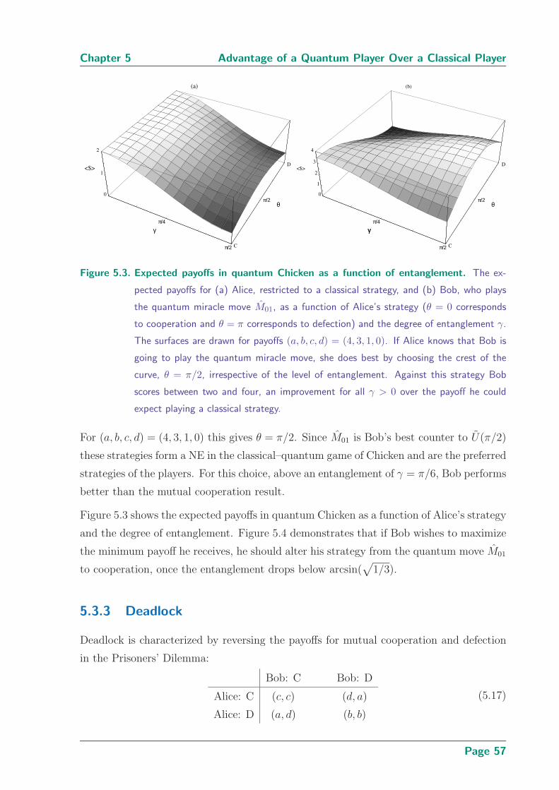
Chapter 5 Advantage of a Quantum Player Over a Classical Player
(a)
π/4
π/2
γ
C
π/2
D
θ
0
1
2
<$>
(b)
π/4
π/2
γ
C
π/2
D
θ
0 1
2
3
4
<$>
γ
Figure 5.3. Expected payoffs in quantum Chicken as a function of entanglement. The ex-
pected payoffs for (a) Alice, restricted to a classical strategy, and (b) Bob, who plays
the quantum miracle move M01, as a function of Alice’s strategy (θ = 0 corresponds
to cooperation and θ = π corresponds to defection) and the degree of entanglement γ.
The surfaces are drawn for payoffs (a, b, c, d) = (4, 3, 1, 0). If Alice knows that Bob is
going to play the quantum miracle move, she does best by choosing the crest of the
curve, θ = π/2, irrespective of the level of entanglement. Against this strategy Bob
scores between two and four, an improvement for all γ > 0 over the payoff he could
expect playing a classical strategy.
For (a, b, c, d) = (4, 3, 1, 0) this gives θ = π/2. Since M01 is Bob’s best counter to U(π/2)
these strategies form a NE in the classical–quantum game of Chicken and are the preferred
strategies of the players. For this choice, above an entanglement of γ = π/6, Bob performs
better than the mutual cooperation result.
Figure 5.3 shows the expected payoffs in quantum Chicken as a function of Alice’s strategy
and the degree of entanglement. Figure 5.4 demonstrates that if Bob wishes to maximize
the minimum payoff he receives, he should alter his strategy from the quantum move M01
to cooperation, once the entanglement drops below arcsin(√
1/3).
5.3.3 Deadlock
Deadlock is characterized by reversing the payoffs for mutual cooperation and defection
in the Prisoners’ Dilemma:
Bob: C Bob: D
Alice: C (c, c) (d, a)
Alice: D (a, d) (b, b)
(5.17)
Page 57
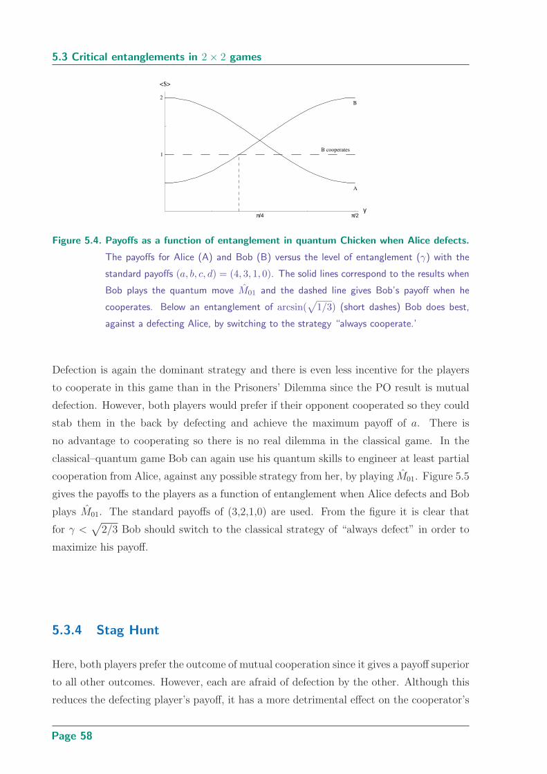
5.3 Critical entanglements in 2 × 2 games
π/4 π/2γ
1
2
<$>
A
B
B cooperates
Figure 5.4. Payoffs as a function of entanglement in quantum Chicken when Alice defects.
The payoffs for Alice (A) and Bob (B) versus the level of entanglement (γ) with the
standard payoffs (a, b, c, d) = (4, 3, 1, 0). The solid lines correspond to the results when
Bob plays the quantum move M01 and the dashed line gives Bob’s payoff when he
cooperates. Below an entanglement of arcsin(√
1/3) (short dashes) Bob does best,
against a defecting Alice, by switching to the strategy “always cooperate.’
Defection is again the dominant strategy and there is even less incentive for the players
to cooperate in this game than in the Prisoners’ Dilemma since the PO result is mutual
defection. However, both players would prefer if their opponent cooperated so they could
stab them in the back by defecting and achieve the maximum payoff of a. There is
no advantage to cooperating so there is no real dilemma in the classical game. In the
classical–quantum game Bob can again use his quantum skills to engineer at least partial
cooperation from Alice, against any possible strategy from her, by playing M01. Figure 5.5
gives the payoffs to the players as a function of entanglement when Alice defects and Bob
plays M01. The standard payoffs of (3,2,1,0) are used. From the figure it is clear that
for γ <√
2/3 Bob should switch to the classical strategy of “always defect” in order to
maximize his payoff.
5.3.4 Stag Hunt
Here, both players prefer the outcome of mutual cooperation since it gives a payoff superior
to all other outcomes. However, each are afraid of defection by the other. Although this
reduces the defecting player’s payoff, it has a more detrimental effect on the cooperator’s
Page 58
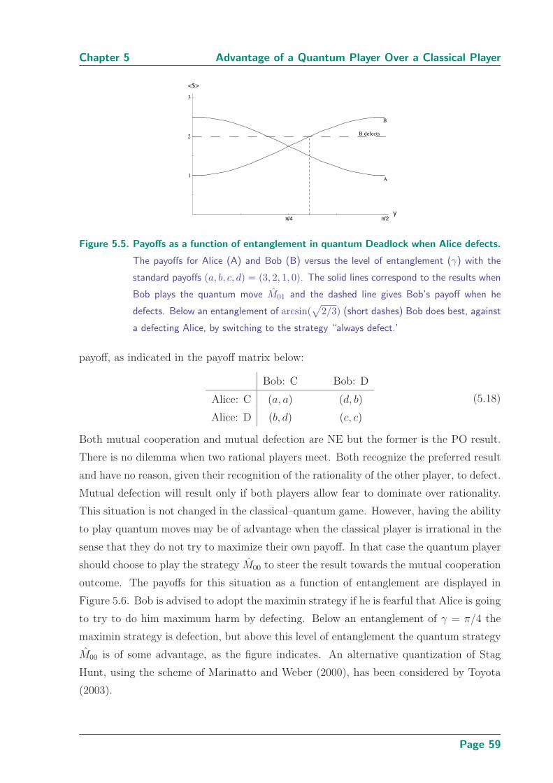
Chapter 5 Advantage of a Quantum Player Over a Classical Player
π/4 π/2γ
1
2
3
<$>
A
B
B defects
Figure 5.5. Payoffs as a function of entanglement in quantum Deadlock when Alice defects.
The payoffs for Alice (A) and Bob (B) versus the level of entanglement (γ) with the
standard payoffs (a, b, c, d) = (3, 2, 1, 0). The solid lines correspond to the results when
Bob plays the quantum move M01 and the dashed line gives Bob’s payoff when he
defects. Below an entanglement of arcsin(√
2/3) (short dashes) Bob does best, against
a defecting Alice, by switching to the strategy “always defect.’
payoff, as indicated in the payoff matrix below:
Bob: C Bob: D
Alice: C (a, a) (d, b)
Alice: D (b, d) (c, c)
(5.18)
Both mutual cooperation and mutual defection are NE but the former is the PO result.
There is no dilemma when two rational players meet. Both recognize the preferred result
and have no reason, given their recognition of the rationality of the other player, to defect.
Mutual defection will result only if both players allow fear to dominate over rationality.
This situation is not changed in the classical–quantum game. However, having the ability
to play quantum moves may be of advantage when the classical player is irrational in the
sense that they do not try to maximize their own payoff. In that case the quantum player
should choose to play the strategy M00 to steer the result towards the mutual cooperation
outcome. The payoffs for this situation as a function of entanglement are displayed in
Figure 5.6. Bob is advised to adopt the maximin strategy if he is fearful that Alice is going
to try to do him maximum harm by defecting. Below an entanglement of γ = π/4 the
maximin strategy is defection, but above this level of entanglement the quantum strategy
M00 is of some advantage, as the figure indicates. An alternative quantization of Stag
Hunt, using the scheme of Marinatto and Weber (2000), has been considered by Toyota
(2003).
Page 59
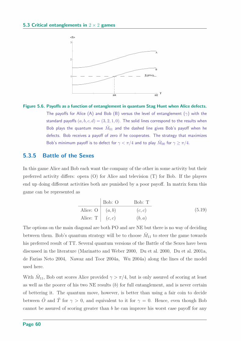
5.3 Critical entanglements in 2 × 2 games
π/4 π/2γ
1
2
3
<$>
A
B
B defects
Figure 5.6. Payoffs as a function of entanglement in quantum Stag Hunt when Alice defects.
The payoffs for Alice (A) and Bob (B) versus the level of entanglement (γ) with the
standard payoffs (a, b, c, d) = (3, 2, 1, 0). The solid lines correspond to the results when
Bob plays the quantum move M01 and the dashed line gives Bob’s payoff when he
defects. Bob receives a payoff of zero if he cooperates. The strategy that maximizes
Bob’s minimum payoff is to defect for γ < π/4 and to play M00 for γ ≥ π/4.
5.3.5 Battle of the Sexes
In this game Alice and Bob each want the company of the other in some activity but their
preferred activity differs: opera (O) for Alice and television (T) for Bob. If the players
end up doing different activities both are punished by a poor payoff. In matrix form this
game can be represented as
Bob: O Bob: T
Alice: O (a, b) (c, c)
Alice: T (c, c) (b, a)
(5.19)
The options on the main diagonal are both PO and are NE but there is no way of deciding
between them. Bob’s quantum strategy will be to choose M11 to steer the game towards
his preferred result of TT. Several quantum versions of the Battle of the Sexes have been
discussed in the literature (Marinatto and Weber 2000, Du et al. 2000, Du et al. 2001a,
de Farias Neto 2004, Nawaz and Toor 2004a, Wu 2004a) along the lines of the model
used here.
With M11, Bob out scores Alice provided γ > π/4, but is only assured of scoring at least
as well as the poorer of his two NE results (b) for full entanglement, and is never certain
of bettering it. The quantum move, however, is better than using a fair coin to decide
between O and T for γ > 0, and equivalent to it for γ = 0. Hence, even though Bob
cannot be assured of scoring greater than b he can improve his worst case payoff for any
Page 60

Chapter 5 Advantage of a Quantum Player Over a Classical Player
(a)
π/4
π/2
γ
O
π/2
T
θ
0
1
<$>
π/4
π/2
(b)
π/4
π/2
O
π/2
T
θ
0
1
2
<$>
γ
Figure 5.7. Expected payoffs in quantum Battle of the Sexes as a function of entanglement.
The expected payoffs for (a) Alice, restricted to a classical strategy, and (b) Bob, who
plays the quantum miracle move M01, as a function of Alice’s strategy (θ = 0 corre-
sponds to opera and θ = π corresponds to television) and the degree of entanglement
γ. The surfaces are drawn for payoffs (a, b, c) = (2, 1, 0). If Alice knows that Bob is
going to play the quantum miracle move, she does best by choosing the crest of the
curve, so her optimal strategy changes from O for no entanglement, to θ = π/2 for
full entanglement. Against this strategy, Bob starts to score better than one for an
entanglement exceeding approximately π/5.
γ > 0. Figure 5.7 shows the payoffs in quantum Battle of Sexes as a function of the degree
of entanglement and Alice’s strategy.
5.4 Extensions
The situation is more complex for multiplayer games. No longer can a quantum player
playing against classical ones engineer any desired final state, even if the opponents’ moves
are known. However, a player can never be worse by having access to the quantum domain
since this includes the classical possibilities as a subset.
In two player games with more than two pure classical strategies the prospects for the
quantum player are better. Some entangled, quantum 3 × 3 games have been considered
in the literature (Iqbal and Toor 2002d, Flitney and Abbott 2002c). Here the full set of
quantum strategies is SU(3) and there are nine possible miracle moves (before considering
symmetries). The strategies that do not manipulate the phase of the player’s qutrit (i.e.,
classical strategies) can be written as the product of three rotations, each parameterized
Page 61
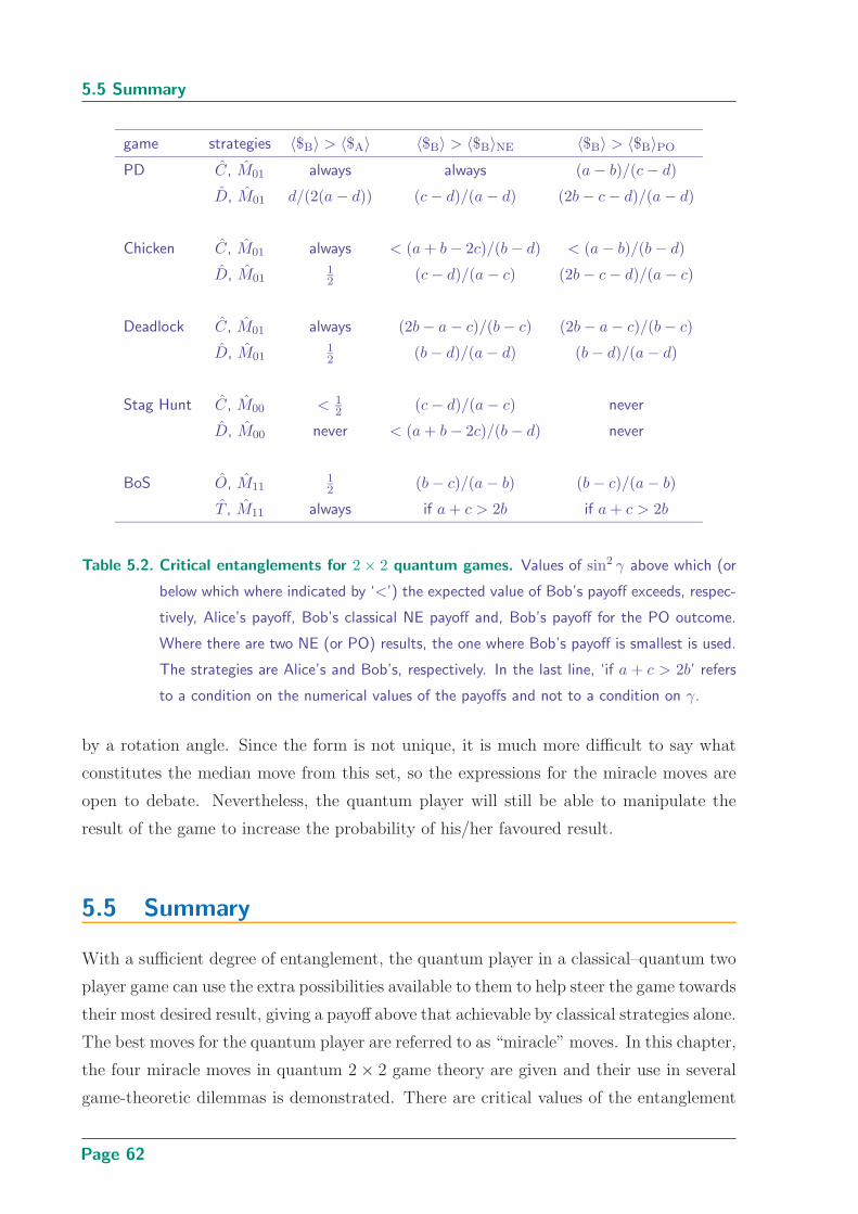
5.5 Summary
game strategies 〈$B〉 > 〈$A〉 〈$B〉 > 〈$B〉NE 〈$B〉 > 〈$B〉PO
PD C, M01 always always (a − b)/(c − d)
D, M01 d/(2(a − d)) (c − d)/(a − d) (2b − c − d)/(a − d)
Chicken C, M01 always < (a + b − 2c)/(b − d) < (a − b)/(b − d)
D, M0112 (c − d)/(a − c) (2b − c − d)/(a − c)
Deadlock C, M01 always (2b − a − c)/(b − c) (2b − a − c)/(b − c)
D, M0112 (b − d)/(a − d) (b − d)/(a − d)
Stag Hunt C, M00 < 12 (c − d)/(a − c) never
D, M00 never < (a + b − 2c)/(b − d) never
BoS O, M1112 (b − c)/(a − b) (b − c)/(a − b)
T , M11 always if a + c > 2b if a + c > 2b
Table 5.2. Critical entanglements for 2 × 2 quantum games. Values of sin2 γ above which (or
below which where indicated by ‘<’) the expected value of Bob’s payoff exceeds, respec-
tively, Alice’s payoff, Bob’s classical NE payoff and, Bob’s payoff for the PO outcome.
Where there are two NE (or PO) results, the one where Bob’s payoff is smallest is used.
The strategies are Alice’s and Bob’s, respectively. In the last line, ‘if a + c > 2b’ refers
to a condition on the numerical values of the payoffs and not to a condition on γ.
by a rotation angle. Since the form is not unique, it is much more difficult to say what
constitutes the median move from this set, so the expressions for the miracle moves are
open to debate. Nevertheless, the quantum player will still be able to manipulate the
result of the game to increase the probability of his/her favoured result.
5.5 Summary
With a sufficient degree of entanglement, the quantum player in a classical–quantum two
player game can use the extra possibilities available to them to help steer the game towards
their most desired result, giving a payoff above that achievable by classical strategies alone.
The best moves for the quantum player are referred to as “miracle” moves. In this chapter,
the four miracle moves in quantum 2 × 2 game theory are given and their use in several
game-theoretic dilemmas is demonstrated. There are critical values of the entanglement
Page 62
Chapter 5 Advantage of a Quantum Player Over a Classical Player
parameter γ below (or occasionally above) which it is no longer an advantage to have
access to quantum moves, that is, where the quantum player can no longer outscore
his/her classical Nash equilibrium result. These represent a phase-like transition in the
classical–quantum game, where a switch between the quantum miracle move and the
dominant classical strategy is warranted. Table 5.2 summarizes the threshold values of γ.
With typical values for the payoffs and a classical player opting for his/her best strategy,
the critical value for sin γ is√
1/3 for Chicken,√
1/5 for Prisoners’ Dilemma and√
2/3
for Deadlock, while for Stag Hunt there is no particular advantage to the quantum player
unless the classical player is adopting a non-optimal strategy. In the Battle of the Sexes
there is no clear threshold but for any non-zero entanglement Bob can improve upon the
possible worst case result that could arise if he was restricted to classical strategies.
The quantum player’s advantage is not as strong in classical–quantum multiplayer games
but in multi-strategy, two player games, depending on the level of entanglement, the
quantum player would again have access to moves that improve his/her result. The
calculation of these moves is problematic because of the larger number of degrees of
freedom and has not been attempted here.
Page 63

Page 64

Chapter 6
Decoherence in QuantumGames
DECOHERENCE in a quantum system results from the inter-
action of the system with its environment. The study of the
effect of decoherence is necessary in any practical quantum in-
formation processing scheme. This chapter presents a scheme for including
decoherence in Eisert’s model of quantum games. The effect of decoherence
is quantified by considering the diminution of the advantage obtainable by a
quantum player against a classical one in several well known 2 × 2 games as
decoherence is increased. The current chapter complements Chapter 5 that
considers how the quantum player’s advantage is affected by the initial degree
of entanglement between the players’ qubits.
Page 65

6.1 Introduction
6.1 Introduction
Decoherence can be defined as non-unitary dynamics resulting from the coupling of the
system with the environment. In any realistic quantum computer, interaction with the
environment cannot be entirely eliminated. Although realization of quantum computers
is debated, steady progress towards this ultimate goal continues (Abbott et al. 2003).
Decoherence can destroy the special features of quantum computation. A review of the
standard mechanisms of quantum decoherence can be found in Zurek (2003). Quantum
computing in the presence of noise is possible with the use of quantum error correction
(Preskill 1998) or decoherence free subspaces (Lidar and Whaley 2003). These techniques
work by encoding the logical qubits in a number of physical qubits. Quantum error correc-
tion is successful, provided the error rate is low enough, while decoherence free subspaces
control certain types of decoherence. Both have the disadvantage of expanding the num-
ber of qubits required for a calculation. Without such measures, the theory of quantum
control in the presence of noise and decoherence is little studied. This motivates the
study of quantum games, which can be viewed as a game-theoretic approach to quantum
control—game-theoretic methods in classical control theory (Carraro and Filar 1995) are
well-established and translating them to the quantum realm is a promising area of study.
Johnson (2001) has considered a three player quantum game corrupted by selecting an
initial state of |111〉 instead of |000〉, with some probability. Above a certain level of
corruption it was found that quantum effects impede the players to such a degree that
they were better off playing the classical game. The same result was found for various
2×2 quantum games with bit flip errors in the initial state (Ozdemir et al. 2004). Chen et
al. (2003b) have discussed decoherence in quantum Prisoners’ Dilemma. Decoherence was
found to have no effect on the NE in this model. The current chapter presents a model
for incorporating decoherence in N -player quantum games of the scheme of Benjamin and
Hayden (2001b). Results for two player Prisoners’ Dilemma, Chicken and the Battle of
the Sexes are calculated as examples.
It is most convenient to use the density matrix notation for the state of the system and
the operator sum representation for the quantum operators. Decoherence can take many
forms including dephasing, which randomizes the relative phases of the quantum states,
and dissipation, that modifies the populations of the quantum states. Pure dephasing of
a qubit can be expressed by
a|0〉 + b|1〉 → a|0〉 + b eiφ|1〉. (6.1)
Page 66
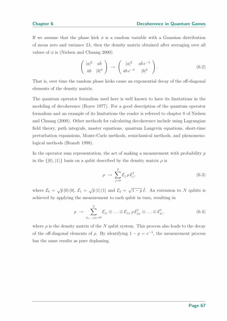
Chapter 6 Decoherence in Quantum Games
If we assume that the phase kick φ is a random variable with a Gaussian distribution
of mean zero and variance 2λ, then the density matrix obtained after averaging over all
values of φ is (Nielsen and Chuang 2000)
(
|a|2 ab
ab |b|2
)
→(
|a|2 ab e−λ
ab e−λ |b|2
)
. (6.2)
That is, over time the random phase kicks cause an exponential decay of the off-diagonal
elements of the density matrix.
The quantum operator formalism used here is well known to have its limitations in the
modeling of decoherence (Royer 1977). For a good description of the quantum operator
formalism and an example of its limitations the reader is referred to chapter 8 of Nielsen
and Chuang (2000). Other methods for calculating decoherence include using Lagrangian
field theory, path integrals, master equations, quantum Langevin equations, short-time
perturbation expansions, Monte-Carlo methods, semiclassical methods, and phenomeno-
logical methods (Brandt 1998).
In the operator sum representation, the act of making a measurement with probability p
in the |0〉, |1〉 basis on a qubit described by the density matrix ρ is
ρ →2∑
j=0
Ej ρ E†j , (6.3)
where E0 =√
p |0〉〈0|, E1 =√
p |1〉〈1| and E2 =√
1 − p I. An extension to N qubits is
achieved by applying the measurement to each qubit in turn, resulting in
ρ →2∑
j1,...,jN=0
Ej1 ⊗ . . . ⊗ EjNρ E†
jN⊗ . . . ⊗ E†
j1, (6.4)
where ρ is the density matrix of the N qubit system. This process also leads to the decay
of the off-diagonal elements of ρ. By identifying 1 − p = e−λ, the measurement process
has the same results as pure dephasing.
Page 67
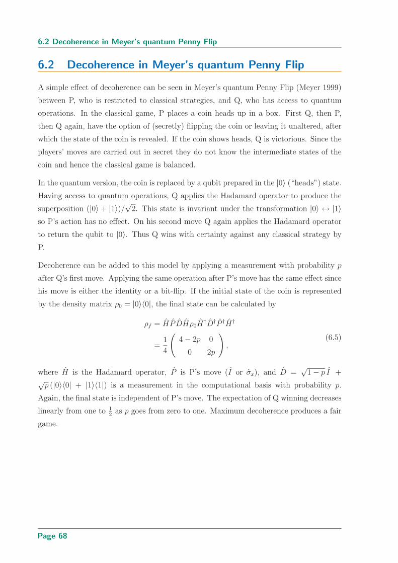
6.2 Decoherence in Meyer’s quantum Penny Flip
6.2 Decoherence in Meyer’s quantum Penny Flip
A simple effect of decoherence can be seen in Meyer’s quantum Penny Flip (Meyer 1999)
between P, who is restricted to classical strategies, and Q, who has access to quantum
operations. In the classical game, P places a coin heads up in a box. First Q, then P,
then Q again, have the option of (secretly) flipping the coin or leaving it unaltered, after
which the state of the coin is revealed. If the coin shows heads, Q is victorious. Since the
players’ moves are carried out in secret they do not know the intermediate states of the
coin and hence the classical game is balanced.
In the quantum version, the coin is replaced by a qubit prepared in the |0〉 (“heads”) state.
Having access to quantum operations, Q applies the Hadamard operator to produce the
superposition (|0〉 + |1〉)/√
2. This state is invariant under the transformation |0〉 ↔ |1〉so P’s action has no effect. On his second move Q again applies the Hadamard operator
to return the qubit to |0〉. Thus Q wins with certainty against any classical strategy by
P.
Decoherence can be added to this model by applying a measurement with probability p
after Q’s first move. Applying the same operation after P’s move has the same effect since
his move is either the identity or a bit-flip. If the initial state of the coin is represented
by the density matrix ρ0 = |0〉〈0|, the final state can be calculated by
ρf = HP DHρ0H†D†P †H†
=1
4
(
4 − 2p 0
0 2p
)
,(6.5)
where H is the Hadamard operator, P is P’s move (I or σx), and D =√
1 − p I +√
p (|0〉〈0| + |1〉〈1|) is a measurement in the computational basis with probability p.
Again, the final state is independent of P’s move. The expectation of Q winning decreases
linearly from one to 12
as p goes from zero to one. Maximum decoherence produces a fair
game.
Page 68

Chapter 6 Decoherence in Quantum Games
6.3 Decoherence in the Eisert scheme
6.3.1 The model
A quantum game in the Eisert scheme with decoherence can be described in the following
manner
ρi ≡ρ0 = |ψ0〉〈ψ0| (initial state) (6.6)
ρ1 = Jρ0J† (entanglement)
ρ2 = D(ρ1, p1) (partial decoherence)
ρ3 = (⊗Nk=1Mk) ρ2 (⊗N
k=1Mk)† (players’ moves)
ρ4 = D(ρ3, p2) (partial decoherence)
ρ5 = J†ρ4J (dis-entanglement),
to produce the final state ρf ≡ ρ5 upon which a measurement is taken. The function
D(ρ, p) is a completely positive map that applies some form of decoherence to the state
ρ controlled by the probability p. The scheme is shown in Figure 6.1. The expectation
value of the payoff for the kth player is
〈$k〉 =∑
ξ
Pξ ρf P†ξ $k
ξ , (6.7)
where Pξ = |ξ〉〈ξ| is the projector onto the state |ξ〉, $kξ is the payoff to the kth player
when the final state is |ξ〉, and the summation is taken over ξ = j1j2 . . . jN , ji = 0, 1.
After choosing Eq. (6.4) to represent the function D in Eq. (6.6) we are now in a position
to write down the results of decoherence in a 2 × 2 quantum game. The notation for
the players’ strategies is given in Eq. (2.9) with, here, the addition of the subscripts A
and B to indicate the parameters of the two traditional protagonists, Alice and Bob,
respectively. Writing ck ≡ cos(θk/2) and sk ≡ sin(θk/2) for k ∈ A,B, the expectation
Page 69

6.3 Decoherence in the Eisert scheme
value of a player’s payoff is
〈$〉 =1
2(c2
Ac2B + s2
As2B)($00 + $11) +
1
2(c2
As2B + s2
Ac2B)($01 + $10)
+1
2(1 − p1)
2(1 − p2)2
[ c2Ac2
B cos(2αA + 2αB) − s2As2
B cos(2βA + 2βB)]($00 − $11)
+ [ c2As2
B cos(2αA − 2βB) − s2Ac2
B cos(2αB − 2βA)]($01 − $10)
+1
4sin θA sin θB
[(1 − p1)
2 sin(αA + αB − βA − βB)(−$00 + $01 + $10 − $11)
+ (1 − p2)2 sin(αA + αB + βA + βB)($00 − $11)
+(1 − p2)2 sin(αA − αB + βA − βB)($10 − $01)
],
(6.8)
where $ij is the payoff to the player for the final state |ij〉. Setting p1 = p2 = 0 gives the
well known result of the Eisert scheme. If in addition, αk = βk = 0, k ∈ A,B, a 2 × 2
classical game results with the mixing between the two classical pure strategies I and F
being determined by θA and θB for Alice and Bob, respectively. Maximum decoherence
with p1 = p2 = 1 gives a result where the quantum phases αk and βk are not relevant:
〈$〉 =x
2($00 + $11) +
1 − x
2($01 + $10), (6.9)
where x = c2Ac2
B + s2As2
B. In this case, a symmetric game yields payoffs to both players
that are the identical. The game is not equivalent to the original classical game. Extrema
for the payoffs occur when both θ’s are 0 or π.
One way of measuring the “quantum-ness” of the game is to consider the known advantage
of a player having access to the full set of quantum strategies Sq over a player who is limited
to the classical set Scl, as considered in Chapter 5. The classical strategies are those for
which the phases α and β vanish. If Alice is restricted in this way then Eq. (6.8) reduces
to
〈$〉 =x
2($00 + $11) +
1 − x
2($01 + $10)
+1
2(1 − p1)
2(1 − p2)2c2B cos 2αB [c2
A($00 − $11) + s2A($10 − $01)]
−s2B cos 2βB [c2
A($10 − $01) + s2A($00 − $11)]
+1
4sin θA sin θB
[(1 − p1)
2 sin(αB − βB)(−$00 + $01 + $10 − $11)
+(1 − p2)2 sin(αB + βB)($00 + $01 − $10 − $11)
].
(6.10)
Page 70

Chapter 6 Decoherence in Quantum Games
|0〉
|0〉
|0〉
⊗
|ψf〉
J J†U1
U2
UN
......
¶³
µ´
¶³
µ´
D D
y
y
p1
p2
-time
Figure 6.1. Flow of information in a quantum game with decoherence. The flow of information
in an N -person quantum game with decoherence, where Uk is the move of the kth player
and J (J†) is an entangling (dis-entangling) gate. The central horizontal lines are the
players’ qubits and the top and bottom lines are classical random bits with a probability
p1 or p2, respectively, of being 1. Here, D is some form of decoherence controlled by
the classical bits.
6.3.2 Prisoners’ Dilemma
For Prisoners’ Dilemma, the standard payoff matrix is
Bob: C Bob: D
Alice: C (3, 3) (0, 5)
Alice: D (5, 0) (1, 1)
(6.11)
where the numbers in parentheses represent payoffs to Alice and Bob, respectively. The
classical pure strategies are cooperation (C) and defection (D). Defecting gives a better
payoff regardless of the other player’s strategy, so it is a dominant strategy, and mutual
defection is the NE. The well known dilemma arises from the fact that both players would
be better off with mutual cooperation, if this could be engineered. With the payoffs of
Eq. (6.11), the best Bob can do from Eq. (6.10) is to select αB = π/2 and βB = 0. Bob’s
choice of θB will depend on Alice’s choice of θA. He can do no better than θB = π/2 if
he is ignorant of Alice’s strategy12. Figure 6.2 shows the payoffs in quantum Prisoners’
Dilemma as a function of decoherence probability p ≡ p1 = p2 and Alice’s strategy θ ≡ θA
when Bob selects his optimal strategy.
12See Chapter 5 or Flitney and Abbott (2003a) for details of quantum versus classical players.
Page 71

6.3 Decoherence in the Eisert scheme
(a)
0.8
0.6
0.4
0.2p
C
π/2
D
θ
0
1
2
3
<$>
(b)
0.8
0.6
0.4
0.2p
C
π/2
D
θ
0
1
2
3
4
5
<$>
Figure 6.2. Payoffs in quantum Prisoners’ Dilemma with decoherence. Payoffs for (a) Alice
and (b) Bob as a function of decoherence probability p and Alice’s strategy θ (being a
measure of the mixing between cooperation (C) and defection (D) with θ = 0 giving
C and θ = π giving D), when Bob plays the optimum quantum strategy and Alice is
restricted to classical strategies. The decoherence goes from the unperturbed quantum
game at p = 0 to maximum decoherence at p = 1.
6.3.3 Chicken
The standard payoff matrix for the game of Chicken is
Bob: C Bob: D
Alice: C (3,3) (1,4)
Alice: D (4,1) (0,0)
(6.12)
There is no dominant strategy. Both CD and DC are NE, with the former preferred by
Bob and the latter by Alice. Again there is a dilemma since the PO result CC is different
from both NE. As above, Bob’s payoff is optimized by αB = π/2, βB = 0 and θB = π/2.
Figure 6.3 shows the payoffs in quantum Chicken as a function of decoherence probability
p and Alice’s strategy θ.
6.3.4 Battle of the Sexes
One form of the payoff matrix for the Battle of the Sexes is
Bob: O Bob: T
Alice: O (2,1) (0,0)
Alice: T (0,0) (1,2)
(6.13)
Page 72

Chapter 6 Decoherence in Quantum Games
(a)
0.8
0.6
0.4
0.2p
C
π/2
D
θ
0
1
2
<$>
(b)
0.8
0.6
0.4
0.2p
C
π/2
D
θ
0
1
2
3
4
<$>
Figure 6.3. Payoffs in quantum Chicken with decoherence. Payoffs for (a) Alice and (b) Bob
as a function of decoherence probability p and Alice’s strategy θ, when Bob plays the
optimum quantum strategy and Alice is restricted to a classical mixed strategy.
Here the two protagonists must decide on an evening’s entertainment. Alice prefers opera
(O) and Bob television (T), but their primary concern is that they do an activity to-
gether. In the absence of communication there is a coordination problem. A quantum
Bob maximizes his payoff in a competition with a classical Alice by choosing αB = −π/2,
βB = 0 and θB = π/2. By doing so he achieves at least partial coordination irrespective
of Alice’s strategy. Figure 6.4 shows the resulting payoffs for Alice and Bob as a function
of decoherence probability p and Alice’s strategy θ.
6.3.5 General remarks on 2 × 2 games
The optimal strategy for Alice in the three games considered is θ = π (or 0) for Pris-
oners’ Dilemma, or θ = π/2 for Chicken and Battle of the Sexes. Figure 6.5 shows the
expectation value of the payoffs to Alice and Bob as a function of the decoherence prob-
ability p for each of the games when Alice chooses her optimal classical strategy. In all
cases considered, Bob out scores Alice and performs better than his classical NE result13
provided p < 1. The advantage of having access to quantum strategies decreases as p
increases, being minimal above p ≈ 0.5, but is still present for all levels of decoherence
up to the maximum. At maximum decoherence (p = 1), with the selected strategies, the
game result is randomized and the expectation of the payoffs are simply the average over
the four possible results. The results presented in Figures 6.2, 6.3 and 6.4 are comparable
13In the case of Chicken or the Battle of the Sexes there are two NE. The one with the lower payoff
has been chosen.
Page 73

6.4 Summary and open questions
(a)
0.8
0.6
0.4
0.2p
C
π/2
D
θ
0
0.5
1
<$>
(b)
0.8
0.6
0.4
0.2p
C
π/2
D
θ
0
1
2
<$>
Figure 6.4. Payoffs in quantum Battle of the Sexes with decoherence. Payoffs for (a) Alice
and (b) Bob as a function of decoherence probability p and Alice’s strategy θ, when
Bob plays the optimum quantum strategy and Alice is restricted to a classical mixed
strategy.
to the results for different levels of entanglement (Flitney and Abbott 2003a). They are
also consistent with the results of Chen et al. (2003b) who show that with increasing
decoherence the payoffs to both players approach the average of the four payoffs in a
quantum Prisoners’ Dilemma.
6.4 Summary and open questions
A method of introducing decoherence into quantum games has been presented. One mea-
sure of the “quantum-ness” of a quantum game subject to decoherence is the advantage a
quantum player has over a player restricted to classical strategies. As expected, increasing
the amount of decoherence degrades the advantage of the quantum player. However, in
the model considered, this advantage does not entirely disappear until the decoherence
is a maximum. When this occurs in a 2 × 2 symmetric game, the results of the players
are equal. The classical game is not reproduced. The loss of advantage to the quantum
player is very similar to that which occurs when the level of entanglement between the
players’ qubits is reduced.
In multi-player quantum games it is known that new Nash equilibria can arise (Benjamin
and Hayden 2001b). The effect of decoherence on the existence of the new equilibria is
an interesting open question. There has been some work on continuous-variable quantum
games (Li et al. 2002) involving an infinite dimensional Hilbert space. The study of
Page 74

Chapter 6 Decoherence in Quantum Games
0.8 0.6 0.4 0.2 0p
1
2
3
4
<$> (a)
Ch
BoS
PD
0.8 0.6 0.4 0.2 0p
1
2
3
4
<$> (b)
BoS
PD
Ch
Figure 6.5. Payoffs with optimal strategies as a function of decoherence in Prisoners’
Dilemma, Chicken and Battle of the Sexes. Payoffs as a function of decoher-
ence probability p, going from fully decohered on the left (p = 1) to fully coherent on
the right (p = 0), for (a) Alice and (b) Bob for the quantum games Prisoners’ Dilemma
(PD), Chicken (Ch) and the Battle of the Sexes (BoS). Bob plays the optimum quantum
strategy and Alice her best classical counter strategy. As expected, the payoff to the
quantum player, Bob, increases with increasing coherence while Alice performs worse ex-
cept in the case of Battle of the Sexes. This game is a coordination game—both players
do better if they select the same move—and Bob can increasingly engineer coordination
as coherence improves, helping Alice as well as himself.
decoherence in infinite dimensional Hilbert space quantum games would need to go beyond
the simple quantum operator method presented in this chapter and is yet to be considered.
This chapter has focused on static quantum games and so future work on game-theoretic
methods for dynamic quantum systems with different types of decohering noise will be
of great interest. A particular open question will be to compare the behaviour of such
quantum games for (a) the non-Markovian case, where the quantum system is coupled to
a dissipative environment with memory, (b) the Markovian (memoryless) limit where the
correlation times, in the decohering environment, are small compared to the characteristic
time scale of the quantum system.
Page 75
Page 76

Chapter 7
Quantum Parrondo’sGames
PARRONDO games involve an apparent paradox where the mix-
ture of two losing games creates a winning game. Positive results
can be obtained with either periodic or random mixtures. Classical
Parrondo’s games and their relationship to Brownian ratchets have generated
much interest. Meyer and Blumer (2002a) introduced a Parrondo game in the
quantum sphere using the discretized Brownian motion of a particle in one
dimension under the influence of a position-dependent potential. A quantum
Parrondo model with history dependence was formulated in 2000 by Ng and
Abbott (2004). Independently, Lee and Johnson (2002a) have suggested a
method of exploiting Parrondo-like effects to generate quantum algorithms.
This chapter presents a summary of the classical Parrondo games and details
of the quantum versions. Some new calculations for both quantum models are
presented. For the position-dependent quantum Parrondo game, the net gain
resulting from various periodic sequences of the two games and for different
parameter values is presented. Short sequences in the history-dependent quan-
tum Parrondo game are studied and comparisons with the equivalent classical
sequences are made.
Page 77
7.1 Introduction
7.1 Introduction
Parrondo’s game is the name given to an apparent paradox that can arise from the mixing
of two games of chance (Parrondo 1996). The defining feature of a Parrondo game is that
a homogeneous sequence of either game gives rise to a losing process, while a random
mixed sequence, or various periodic sequences, of the two games results in a winning
process. The effect was first explored as a combination of two gambling games involving
the use of biased coins (Harmer and Abbott 1999a).
The classical Parrondo game consists of two sub-games A and B. In the usual scenario,
game A is the toss of a single biased coin, while game B utilizes two or more biased coins,
the choice of which depends on the game situation. To obtain Parrondian behaviour, a
form of feedback from the current game state is required. This can take the form of a
dependence on the total capital (Harmer and Abbott 1999b), on past results (Parrondo et
al. 2000), on the spatial neighbourhood (Toral 2001), or on spatial extension (Masuda and
Kondo 2004). The capital- and history-dependent Parrondo games are the most intensely
studied and the basic formalism is described in a number of papers (Harmer et al. 2000,
Harmer and Abbott 2002, Johnson et al. 2003, Kay and Johnson 2003, Harmer et al.
2004).
A ratchet and pawl driven in one direction by the random thermal motion of the surround-
ing particles is discussed by Feynman et al. (1963). At thermal equilibrium, this is ruled
out by the second law of thermodynamics, however, with a Brownian ratchet (Reimann
2002) or flashing ratchet (Doering 1995) directed motion can be obtained from random
fluctuations or noise in the absence of systematic macroscopic forces. The flashing ratchet,
consisting of a Brownian particle under the influence of a potential that is switched on or
off either periodically or stochastically, provides a physical model for Parrondo’s games
(Harmer and Abbott 2001, Allison and Abbott 2002, Toral et al. 2003b). Classical
Parrondo’s games appear to be ubiquitous14 and there is speculation that they may arise
in many areas including population genetics (McClintock 1999), spin systems (Moraal
2000), control systems (Allison and Abbott 2001), biological systems at the molecular
level (Astumian 2001), biogenesis (Davies 2001), and evolutionary processes (Abbott et
al. 2002). There is even a suggestion of a profitable stockmarket trading strategy ex-
ploiting Parrondo’s games (Klarreich 2001a). In all these examples the combination of
processes leads to counterintuitive dynamics.
14Furthermore see Costa et al. (2004) where it is argued that ubiquity is the rule rather than the
exception.
Page 78
Chapter 7 Quantum Parrondo’s Games
A quantum Parrondo game is a translation of the Parrondo effect into the quantum world.
Quantum interference effects provide a mechanism, in additional to the classical feedback,
that can enhance or inhibit the Parrondo effect. Quantum systems that are analogous
to the capital- and the history-dependent Parrondo games have been proposed (Flitney
et al. 2002, Meyer and Blumer 2002a, Ng and Abbott 2004) as well as other uniquely
quantum variants (Lee et al. 2002).
7.2 Classical Parrondo’s games
7.2.1 Capital-dependent games
In capital-dependent Parrondo’s games, game A is the toss of a single biased coin with
winning probability p = 1/2 − ǫ, for some small ǫ > 0, while game B employs two coins
whose use depends on the total capital of the player: coin B1 with winning probability p1
is used if the capital is divisible by three, otherwise B2 is used with winning probability
p2. This situation is shown schematically in Figure 7.1. By choosing, for example,
p1 = 1/10 − ǫ, p2 = 3/4 − ǫ, ǫ > 0, (7.1)
a net loss over time is generated (Harmer and Abbott 1999b). Although the weighted
average of the winning probabilities in Eq. (7.1) is positive for small ǫ, the “bad” coin
B1 is used more often than the one-third of the time that might naively be expected. By
mixing games A and B this effect is broken and the combination can now be winning
provided the net positive effect of game B exceeds the negative bias of game A. Figure 7.2
shows the expected results over 100 coin tosses for some deterministic sequences of games
A and B as well as the random sequence where the choice of game to be played at each
step is determined by a fair coin.
7.2.2 History-dependent games
In the classical history dependent Parrondo’s paradox, game A is as above, while game
B is a collection of biased coins, the selection of which is dependent on the results of
previous games as indicated in Figure 7.3. In order to obtain Parrondian behaviour, a
dependence on at least the previous two results is necessary. An analysis of game B shows
it to be losing for ǫ > 0 when we choose (Parrondo et al. 2000)
p1 = 9/10 − ǫ, p2 = p3 = 1/4 − ǫ, p4 = 7/10 − ǫ. (7.2)
Page 79
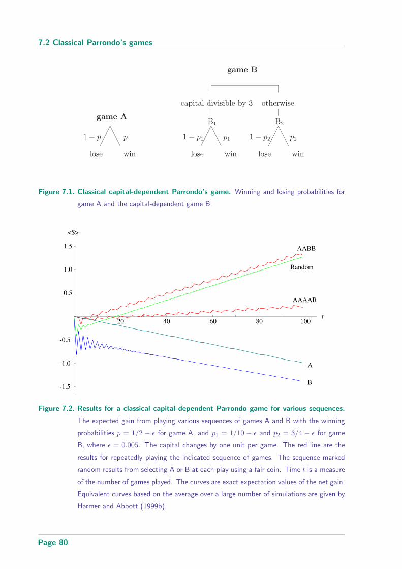
7.2 Classical Parrondo’s games
game A
¢¢¢A
AA
1 − p p
lose win
game B
capital divisible by 3
B1
¢¢¢A
AA
1 − p1 p1
lose win
otherwise
B2
¢¢¢A
AA
1 − p2 p2
lose win
Figure 7.1. Classical capital-dependent Parrondo’s game. Winning and losing probabilities for
game A and the capital-dependent game B.
20
40
60
80
100
t
-1.5
-1.0
-0.5
0.5
1.0
1.5
<$>
A
B
Random
AABB
AAAAB
Figure 7.2. Results for a classical capital-dependent Parrondo game for various sequences.
The expected gain from playing various sequences of games A and B with the winning
probabilities p = 1/2 − ǫ for game A, and p1 = 1/10 − ǫ and p2 = 3/4 − ǫ for game
B, where ǫ = 0.005. The capital changes by one unit per game. The red line are the
results for repeatedly playing the indicated sequence of games. The sequence marked
random results from selecting A or B at each play using a fair coin. Time t is a measure
of the number of games played. The curves are exact expectation values of the net gain.
Equivalent curves based on the average over a large number of simulations are given by
Harmer and Abbott (1999b).
Page 80
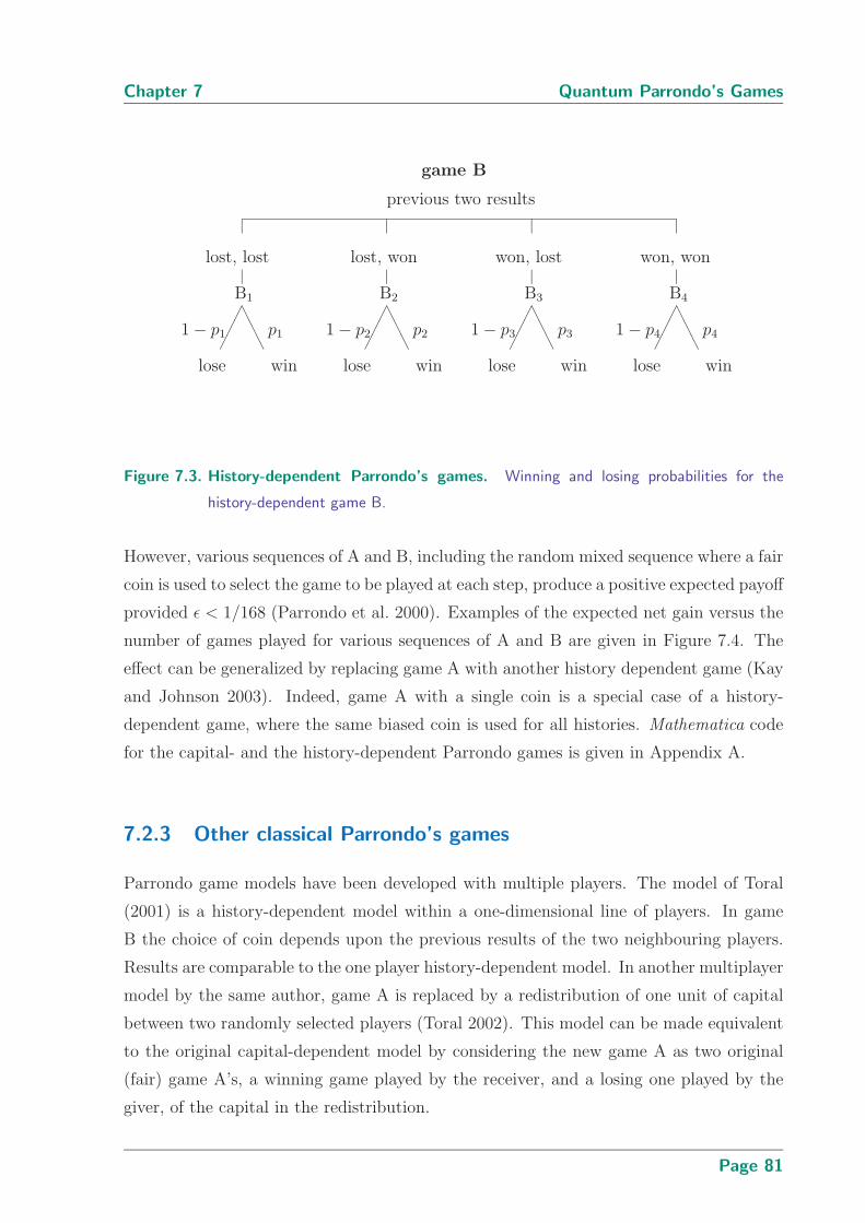
Chapter 7 Quantum Parrondo’s Games
previous two results
game B
lost, lost
B1
¢¢¢A
AA
1 − p1 p1
lose win
lost, won
B2
¢¢¢A
AA
1 − p2 p2
lose win
won, lost
B3
¢¢¢A
AA
1 − p3 p3
lose win
won, won
B4
¢¢¢A
AA
1 − p4 p4
lose win
Figure 7.3. History-dependent Parrondo’s games. Winning and losing probabilities for the
history-dependent game B.
However, various sequences of A and B, including the random mixed sequence where a fair
coin is used to select the game to be played at each step, produce a positive expected payoff
provided ǫ < 1/168 (Parrondo et al. 2000). Examples of the expected net gain versus the
number of games played for various sequences of A and B are given in Figure 7.4. The
effect can be generalized by replacing game A with another history dependent game (Kay
and Johnson 2003). Indeed, game A with a single coin is a special case of a history-
dependent game, where the same biased coin is used for all histories. Mathematica code
for the capital- and the history-dependent Parrondo games is given in Appendix A.
7.2.3 Other classical Parrondo’s games
Parrondo game models have been developed with multiple players. The model of Toral
(2001) is a history-dependent model within a one-dimensional line of players. In game
B the choice of coin depends upon the previous results of the two neighbouring players.
Results are comparable to the one player history-dependent model. In another multiplayer
model by the same author, game A is replaced by a redistribution of one unit of capital
between two randomly selected players (Toral 2002). This model can be made equivalent
to the original capital-dependent model by considering the new game A as two original
(fair) game A’s, a winning game played by the receiver, and a losing one played by the
giver, of the capital in the redistribution.
Page 81
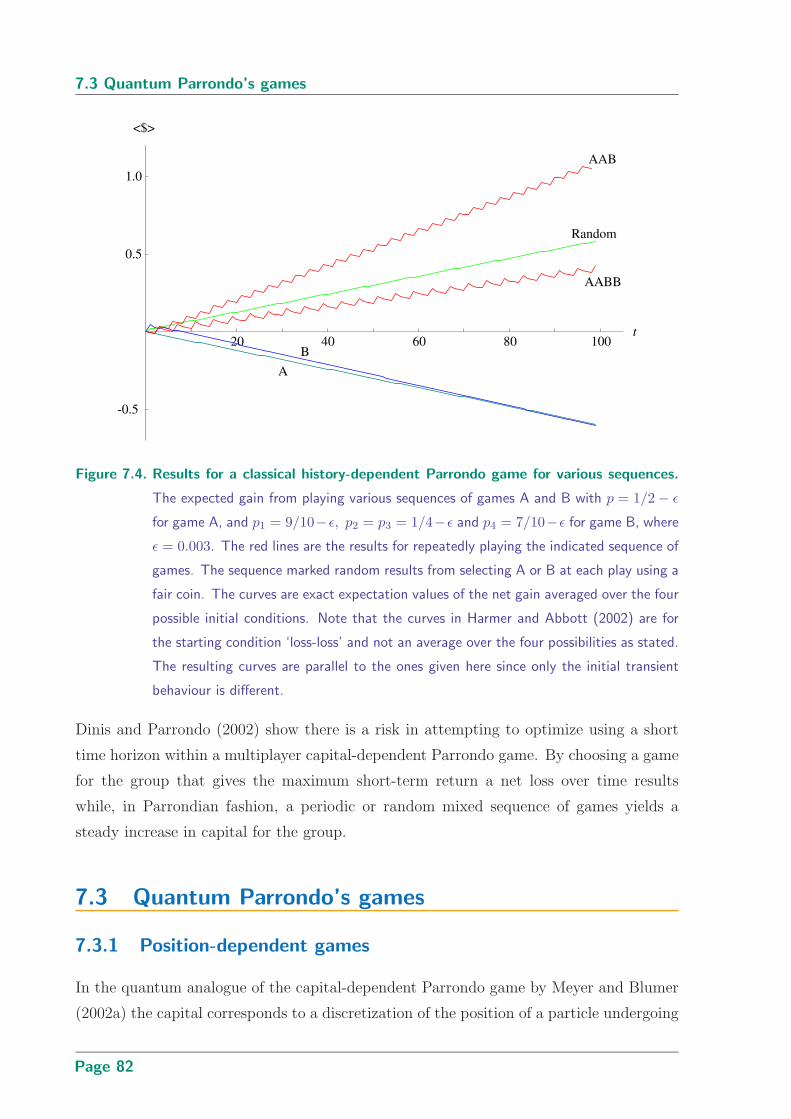
7.3 Quantum Parrondo’s games
20
40
60
80
100
t
-0.5
0.5
1.0
<$>
A
B
Random
AAB
AABB
Figure 7.4. Results for a classical history-dependent Parrondo game for various sequences.
The expected gain from playing various sequences of games A and B with p = 1/2 − ǫ
for game A, and p1 = 9/10−ǫ, p2 = p3 = 1/4−ǫ and p4 = 7/10−ǫ for game B, where
ǫ = 0.003. The red lines are the results for repeatedly playing the indicated sequence of
games. The sequence marked random results from selecting A or B at each play using a
fair coin. The curves are exact expectation values of the net gain averaged over the four
possible initial conditions. Note that the curves in Harmer and Abbott (2002) are for
the starting condition ‘loss-loss’ and not an average over the four possibilities as stated.
The resulting curves are parallel to the ones given here since only the initial transient
behaviour is different.
Dinis and Parrondo (2002) show there is a risk in attempting to optimize using a short
time horizon within a multiplayer capital-dependent Parrondo game. By choosing a game
for the group that gives the maximum short-term return a net loss over time results
while, in Parrondian fashion, a periodic or random mixed sequence of games yields a
steady increase in capital for the group.
7.3 Quantum Parrondo’s games
7.3.1 Position-dependent games
In the quantum analogue of the capital-dependent Parrondo game by Meyer and Blumer
(2002a) the capital corresponds to a discretization of the position of a particle undergoing
Page 82

Chapter 7 Quantum Parrondo’s Games
Brownian motion in one dimension. The application of an appropriate potential produces
the effect of games A or B. A potential uniformly increasing with x is the analogy of
game A, while game B corresponds to a tilted sawtooth potential. The quantum “coin”
is a two state system such as a spin–12
particle, in a superposition of the |R〉 and |L〉states,15 the eigenstates of σz. The quantum analogue of an unbiased coin flip is a unitary
transformation represented by the matrix 1√2
(1 ii 1
). Let |x〉 correspond to the gambling
capital, and |R〉 and |L〉 indicate a win or a loss, respectively. Motion towards increasingly
positive x corresponds to a winning process. An unbiased “coin” flip is effected by the
unitary transformation
|x, L〉 → 1√2
(|x − 1, L〉 + i|x + 1, R〉) ,
|x,R〉 → 1√2
(i|x − 1, L〉 + |x + 1, R〉) .(7.3)
The initial state is chosen to be 1√2(|0, R〉−|0, L〉) so the particle begins with no particular
momentum bias and an unbiased game A produces no net drift16. The effect of the
potentials are implemented by multiplication by an x-dependent phase factor (Meyer
1997). The quantum version of the games is the unbiased transition in Eq. (7.3) multiplied
by a phase e−iV (x) where
VA(x) = αx, (7.4a)
VB(x) = αx + β(1 − 1
2(x mod 3)), (7.4b)
for games A and B, respectively. The potential VB(x) is indicated in Figure 7.5.
The analogy with the classical capital-dependent Parrondo game is not exact. In the
quantum case, for game A 〈x〉 is periodic with period 2π/α. However, game A is losing
in the sense that for α > 0, 〈x〉 ≤ 0 for all times. The situation is similar for game B. For
detail refer to Meyer and Blumer (2002a).
Choosing α = 2π/5000 and β = π/3 gives results for the individual games comparable
(within a factor of two) to the classical games with the probabilities of Eq. (7.1). Repeating
the sequence17 AAAAB produces one of the greatest positive movements of the particle,
15The notation |R〉 and |L〉 is used in preference to |↑〉 and |↓〉 for consistency with Chapter 8.16In Travaglione and Milburn (2002) an unbiased quantum walk is created by using the Hadamard
operator, represented by 1√
2
(1 11 −1
), and starting with the initial state 1
√
2(|0, L〉 + i|0, R〉). The two
schemes are equivalent.17Meyer and Blumer (2002a) indicate that the sequence is BAAAA and this was repeated in the review
by Flitney and Abbott (2003c). This was an error that has now been cleared up: four games of A are
played first (Meyer 2003)—in other words AAAAB is the correct sequence. In fact, the sequence BAAAA
produces net motion in the negative direction.
Page 83
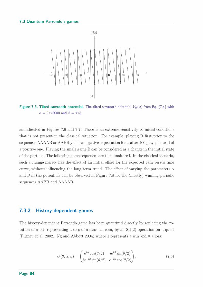
7.3 Quantum Parrondo’s games
-30
-20
-10
10
20
30x
-1
1
V(x)
Figure 7.5. Tilted sawtooth potential. The tilted sawtooth potential VB(x) from Eq. (7.4) with
α = 2π/5000 and β = π/3.
as indicated in Figures 7.6 and 7.7. There is an extreme sensitivity to initial conditions
that is not present in the classical situation. For example, playing B first prior to the
sequences AAAAB or AABB yields a negative expectation for x after 100 plays, instead of
a positive one. Playing the single game B can be considered as a change in the initial state
of the particle. The following game sequences are then unaltered. In the classical scenario,
such a change merely has the effect of an initial offset for the expected gain versus time
curve, without influencing the long term trend. The effect of varying the parameters α
and β in the potentials can be observed in Figure 7.8 for the (mostly) winning periodic
sequences AABB and AAAAB.
7.3.2 History-dependent games
The history-dependent Parrondo game has been quantized directly by replacing the ro-
tation of a bit, representing a toss of a classical coin, by an SU(2) operation on a qubit
(Flitney et al. 2002, Ng and Abbott 2004) where 1 represents a win and 0 a loss:
U(θ, α, β) =
(
eiα cos(θ/2) ieiβ sin(θ/2)
ie−iβ sin(θ/2) e−iα cos(θ/2)
)
, (7.5)
Page 84
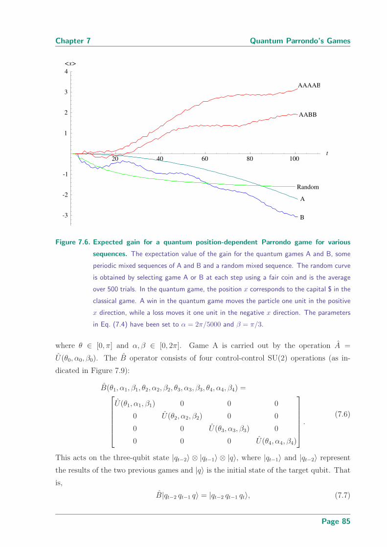
Chapter 7 Quantum Parrondo’s Games
20 40 60 80 100t
-3
-2
-1
1
2
3
4
<x>
A
B
Random
AABB
AAAAB
Figure 7.6. Expected gain for a quantum position-dependent Parrondo game for various
sequences. The expectation value of the gain for the quantum games A and B, some
periodic mixed sequences of A and B and a random mixed sequence. The random curve
is obtained by selecting game A or B at each step using a fair coin and is the average
over 500 trials. In the quantum game, the position x corresponds to the capital $ in the
classical game. A win in the quantum game moves the particle one unit in the positive
x direction, while a loss moves it one unit in the negative x direction. The parameters
in Eq. (7.4) have been set to α = 2π/5000 and β = π/3.
where θ ∈ [0, π] and α, β ∈ [0, 2π]. Game A is carried out by the operation A =
U(θ0, α0, β0). The B operator consists of four control-control SU(2) operations (as in-
dicated in Figure 7.9):
B(θ1, α1, β1, θ2, α2, β2, θ3, α3, β3, θ4, α4, β4) =
U(θ1, α1, β1) 0 0 0
0 U(θ2, α2, β2) 0 0
0 0 U(θ3, α3, β3) 0
0 0 0 U(θ4, α4, β4)
.(7.6)
This acts on the three-qubit state |qt−2〉 ⊗ |qt−1〉 ⊗ |q〉, where |qt−1〉 and |qt−2〉 represent
the results of the two previous games and |q〉 is the initial state of the target qubit. That
is,
B|qt−2 qt−1 q〉 = |qt−2 qt−1 qt〉, (7.7)
Page 85

7.3 Quantum Parrondo’s games
1
2
3
4
5 1
2
3
4
5
b
-2
0
2
4
<x>
1
2
3
4
5
a
Figure 7.7. Expected gain for a quantum position-dependent Parrondo game as a function
of game mixture. The expectation value of the gain after 100 games of a periodic
mixed sequence created by repeating a games of A followed by b games of B, with
α = 2π/5000 and β = π/3. For example, a = 4, b = 1 represents the sequence
AAAAB repeated 20 times, giving a total of 100 games.
π/2 π β
-8
-6
-4
-2
2
4
<x>
α increasing
AABB
π/2
π
β
-8
-6
-4
-2
2
4
<x>
α increasing
AAAAB
Figure 7.8. Expected gain for a quantum position-dependent Parrondo game for various
parameter values in the potentials. The expectation value of the gain after 100
games using the sequence (a) AABB or (b) AAAAB, for various values of α and β.
The curves are for α = 0, α = π/5000, α = π/2500, α = π/1250, and α = π/625,
increasing in the direction indicated.
Page 86
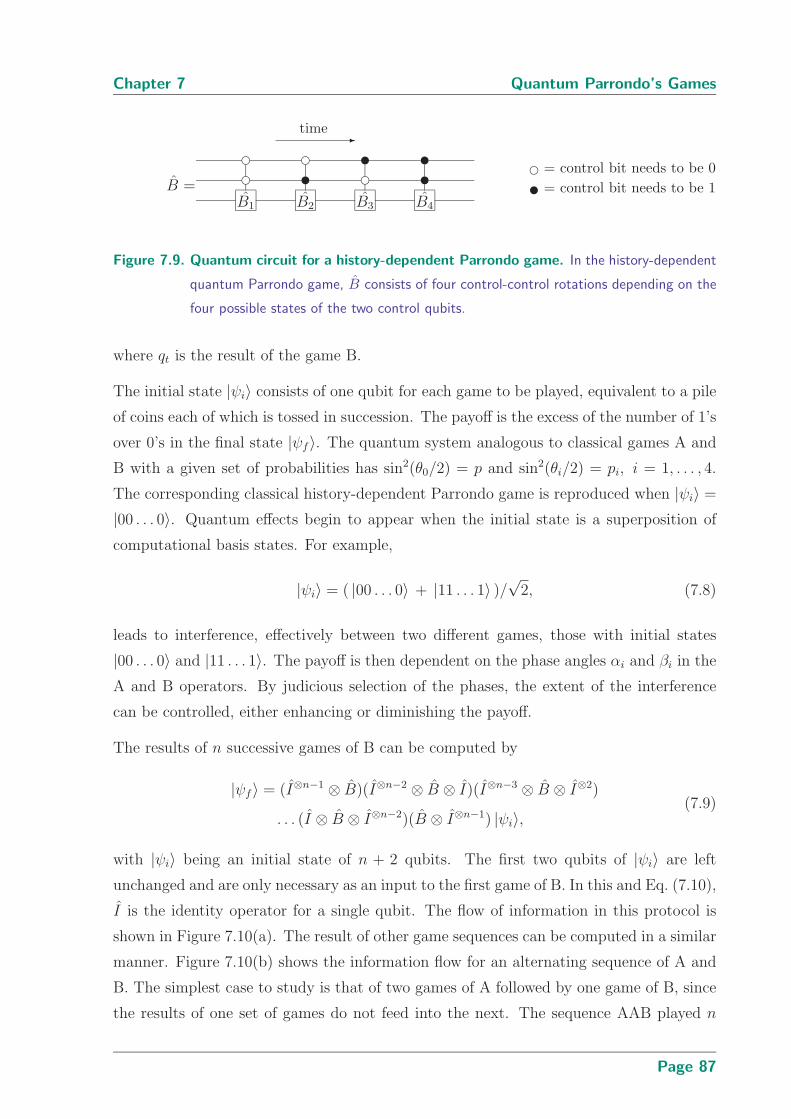
Chapter 7 Quantum Parrondo’s Games
B =B1 B2 B3 B4
ee
eu
ue
uu e
u= control bit needs to be 0
= control bit needs to be 1
-time
Figure 7.9. Quantum circuit for a history-dependent Parrondo game. In the history-dependent
quantum Parrondo game, B consists of four control-control rotations depending on the
four possible states of the two control qubits.
where qt is the result of the game B.
The initial state |ψi〉 consists of one qubit for each game to be played, equivalent to a pile
of coins each of which is tossed in succession. The payoff is the excess of the number of 1’s
over 0’s in the final state |ψf〉. The quantum system analogous to classical games A and
B with a given set of probabilities has sin2(θ0/2) = p and sin2(θi/2) = pi, i = 1, . . . , 4.
The corresponding classical history-dependent Parrondo game is reproduced when |ψi〉 =
|00 . . . 0〉. Quantum effects begin to appear when the initial state is a superposition of
computational basis states. For example,
|ψi〉 = ( |00 . . . 0〉 + |11 . . . 1〉 )/√
2, (7.8)
leads to interference, effectively between two different games, those with initial states
|00 . . . 0〉 and |11 . . . 1〉. The payoff is then dependent on the phase angles αi and βi in the
A and B operators. By judicious selection of the phases, the extent of the interference
can be controlled, either enhancing or diminishing the payoff.
The results of n successive games of B can be computed by
|ψf〉 = (I⊗n−1 ⊗ B)(I⊗n−2 ⊗ B ⊗ I)(I⊗n−3 ⊗ B ⊗ I⊗2)
. . . (I ⊗ B ⊗ I⊗n−2)(B ⊗ I⊗n−1) |ψi〉,(7.9)
with |ψi〉 being an initial state of n + 2 qubits. The first two qubits of |ψi〉 are left
unchanged and are only necessary as an input to the first game of B. In this and Eq. (7.10),
I is the identity operator for a single qubit. The flow of information in this protocol is
shown in Figure 7.10(a). The result of other game sequences can be computed in a similar
manner. Figure 7.10(b) shows the information flow for an alternating sequence of A and
B. The simplest case to study is that of two games of A followed by one game of B, since
the results of one set of games do not feed into the next. The sequence AAB played n
Page 87

7.4 New results for a quantum history-dependent game
times results in the state
|ψf〉 =(
I⊗3n−3 ⊗ (B(A ⊗ A ⊗ I)))
(
I⊗3n−6 ⊗ (B(A ⊗ A ⊗ I)) ⊗ I⊗3)
. . .(
(B(A ⊗ A ⊗ I)) ⊗ I⊗3n−3)
|ψi〉
= G⊗n|ψi〉,
(7.10)
where G = B(A ⊗ A ⊗ I) and |ψi〉 is an initial state of 3n qubits. The information flow
for this sequence is shown in Figure 7.10(c).
To determine the expected gain from a sequence of games let the payoff for a |1〉 state be
one and for a |0〉 state be negative one. If the final state is |ψf〉, the expected gain can
be computed by
〈$〉 =n∑
j=0
(
(2j − n)∑
j′
∣∣∣〈ψj′
j |ψf〉∣∣∣
2)
, (7.11)
where the second summation is taken over all basis states 〈ψj′
j | with j ones and n − j
zeros.
7.4 New results for a quantum history-dependent game
Consider the game sequence AAB. With an initial state of |000〉 this yields a payoff of
〈$0AAB〉 = sin4(θ0/2) (2 − cos θ4) − cos4(θ0/2) (2 + cos θ1)
− 1
4sin2 θ0 (cos θ2 + cos θ3),
(7.12)
which is the same as the classical result. In order to obtain interference there needs to be
two different ways of arriving at the same state. We need only choose an initial state that
is some superposition of the computational basis states, not necessarily the maximally
entangled state, however, it is this that is the most interesting to study. Choosing |ψmi 〉 =
1√2(|000〉 + |111〉) the resulting expected payoff for AAB is
〈$mAAB〉 =
1
2cos θ0 (cos θ4 − cos θ1)
− 1
4sin2 θ0 [sin(2α0 + α1 − 2β0 − β1) sin θ1
− sin(2α0 + α2 − 2β0 − β2) sin θ2 − sin(2α0 + α3 − 2β0 − β3) sin θ3
+ sin(2α0 + α4 − 2β0 − β4) sin θ4] .
(7.13)
Page 88
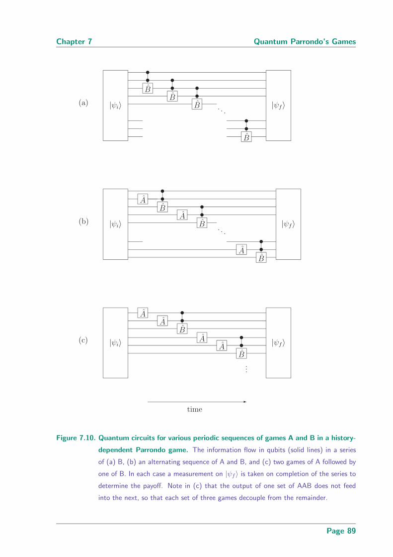
Chapter 7 Quantum Parrondo’s Games
|ψi〉
BB
B . . .
B
|ψf〉
tt
tt
tt
tt
(a)
|ψi〉
A
AB
B . . .
AB
|ψf〉
tt
tt
tt
(b)
|ψi〉
AA
B
B
AA
...
|ψf〉
tt
tt
-
time
(c)
Figure 7.10. Quantum circuits for various periodic sequences of games A and B in a history-
dependent Parrondo game. The information flow in qubits (solid lines) in a series
of (a) B, (b) an alternating sequence of A and B, and (c) two games of A followed by
one of B. In each case a measurement on |ψf 〉 is taken on completion of the series to
determine the payoff. Note in (c) that the output of one set of AAB does not feed
into the next, so that each set of three games decouple from the remainder.
Page 89
7.4 New results for a quantum history-dependent game
It is the dependence on the phase angles αi and βi that permit a result that cannot
be obtained from the classical games. In the quantum case, a range of payoffs can be
obtained for a given set of θ’s (that is, for a given set of probabilities for games A and B)
by adjusting these phase factors.
After choosing θi’s corresponding to the probabilities in Eq. (7.2), the expectation value
of the payoff [to O(ǫ)] in the quantum system for a single sequence of AAB can vary
between 0.812 + 0.24ǫ and −0.812 + 0.03ǫ. The maximum result is obtained by setting
α2 − β2 = α3 − β3 = π/2 − 2α0 + 2β0; (7.14)
α1 − β1 = α4 − β4 = 3π/2 − 2α0 + 2β0,
while the minimum is obtained by
α1 − β1 = α4 − β4 = π/2 − 2α0 + 2β0; (7.15)
α2 − β2 = α3 − β3 = 3π/2 − 2α0 + 2β0.
Classically, AAB is a winning sequence provided ǫ < 1/112. This and other results for
short sequences of games are given in Table 7.1.
The average payoff for the classical game sequence AAB1 (that is, AAB where each branch
of B is the best branch B1) is 45− 6ǫ which is less than the greatest value of 〈$m
AAB〉. Thus
the entanglement and the resulting interference can make game B in the sequence AAB
better than its best branch taken alone! Indeed the expectation value for the payoff of
a quantum AAB1 on the maximally entangled initial state vanishes due to destructive
interference. (This can be seen from Eq. (7.13) by setting θ2, θ3 and θ4 equal to θ1 and
similarly for the α’s and β’s.)
The quantum enhancement disappears when we play a series of AAB’s on the maximally
entangled initial state. In this case the phase dependent terms undergo destructive in-
terference and we are left with a gain per qubit of order ǫ as indicated in the last line of
Table 7.1.
A sequence of B’s leaves the first two qubits unaltered while a sequence of AB’s leaves
the first qubit unaffected. In these cases the final states that arise from |ψi〉 = |000〉 and
|ψi〉 = |111〉 are distinct, so a superposition of these two states produces no interference.
For these sequences, a different superposition for the initial state is required to give rise
to interference effects.
Page 90

Chapter 7 Quantum Parrondo’s Games
sequence classical payoff quantum payoff
AA . . . A −2ǫ 0
B 1/60 − 2ǫ/3 1/15
BB 1/75 − 19ǫ/15 13/400 + ǫ/20
BBB 0.008 − 1.1ǫ 0.017 + 0.03ǫ
AB 1/60 − 19ǫ/15 1/30 + ǫ/15
ABAB 0.032 − 2.5ǫ 0.019 + 0.08ǫ
AAB 1/60 − 28ǫ/15 −0.271 + 0.03ǫ ; 0.271 + 0.24ǫ
AAB . . . AAB 1/60 − 28ǫ/15 2ǫ/15
Table 7.1. Expected payoffs per qubit for various sequences in a history-dependent Par-
rondo game. The classical payoffs are the average over the four possible initial condi-
tions, while the quantum payoffs are calculated for the maximally entangled initial state,
1√2(|00 . . . 0〉 + |11 . . . 1〉). For the sequence AAB the two values given for the quantum
payoff are the minimum and maximum that can be obtained by adjusting the phase
factors in A and B (see text). All payoffs are given to O(ǫ).
7.5 Other quantum Parrondian behaviour
Lee and Johnson consider how decoherence in a quantum system can be suppressed by a
Parrondo-like effect (Lee et al. 2002, Lee and Johnson 2002a). In addition, the authors
approach the construction of Grover’s search algorithm with a view to exploiting Par-
rondian behaviour. In their model “games” A and B represent a partitioning of the steps
in Grover’s search algorithm. Neither step alone is efficient, but by randomly combining
A and B the original algorithm is recreated, thus giving a constructive role to randomness
in the creation of quantum algorithms.
7.6 Summary
Parrondian behaviour arises in the mixing of two games when the surface dividing the
winning and losing regions of the parameter space of the games is convex (Harmer and
Abbott 2002, Harmer et al. 2004). This means that a convex linear combination of two
losing games can become a winning game, or vice versa. Classical Parrondo’s games have
a physical analogue in Brownian or flashing ratchets. A summary of the classical Parrondo
effect has been presented in order to motivate the study of quantum versions. Results
Page 91
7.6 Summary
for both the capital- and history-dependent games have been presented, in the latter case
correcting earlier published results.
A position-dependent quantum Parrondo game has been described (Meyer and Blumer
2002a, Meyer and Blumer 2002b) and new results for various periodic sequences of games
and different parameter values in the biasing potentials have been given. A quantum
version of a history-dependent Parrondo game has been detailed (Flitney et al. 2002, Ng
and Abbott 2004) and the results of short sequences of games presented. If the initial
state is a superposition of basis states, payoffs different from the corresponding classical
game can be obtained as a result of interference. In some cases payoffs can be considerably
altered by adjusting the phase factors associated with the operators without altering the
amplitudes (and hence the associated classical probabilities). If the initial state is simply
|00 . . . 0〉 the payoffs are independent of the phases and are no different from the classical
payoffs. In other cases it is possible to obtain either much larger or smaller payoffs,
provided the initial state involves a superposition that gives the possibility of interference
for that particular game sequence.
In classical gambling games there is a random element. In a Parrondo game the results of
the random process are used to alter the evolution of the game through a form of feedback.
The quantum mechanical model is deterministic until a measurement is made at the end
of the process. The element of chance that is necessary in the classical game is replaced
by a superposition that represents all the possible results in parallel. New behaviour can
arise by the addition of phase factors in the operators and by interference between states.
Another random element, warranting further study, can be introduced by perturbing the
system with noise or decoherence (Meyer 2003).
Classical Parrondo games can be extracted by discretizing the classical Fokker-Planck
equation (Allison and Abbott 2003, Toral et al. 2003a, Amengual et al. 2004). It
is therefore an interesting open question whether the quantum Fokker-Planck equation
(Banik et al. 2002) can be used to generate quantum Parrondo games. In future work, it
will also be interesting to consider whether entanglement alone can provide the coupling
between the games and give rise to quantum Parrondian behaviour.
Page 92
Chapter 8
Quantum Walks withHistory Dependence
Q UANTUM walks are the quantum analogue of classical ran-
dom walks and display some interesting features that make
them a plausible candidate for use in quantum computation.
In this chapter a brief overview of quantum walks and their
main features is presented, before detailing new work on a history-dependent
quantum walk that can give rise to another quantum Parrondo’s game. A
multi-coin discrete-time quantum walk is introduced where the amplitude for
a coin flip depends upon previous results. Although the corresponding history-
dependent classical random walk is unbiased, a bias can be introduced into
the quantum walk by varying the history dependence. By mixing a biased and
an unbiased quantum walk, the direction of the bias can be reversed leading
to a new quantum version of Parrondo’s paradox. Two-, three- and four-coin
history-dependent quantum walks, the effect of the biasing parameters, and
the new quantum Parrondo effect are discussed.
Page 93
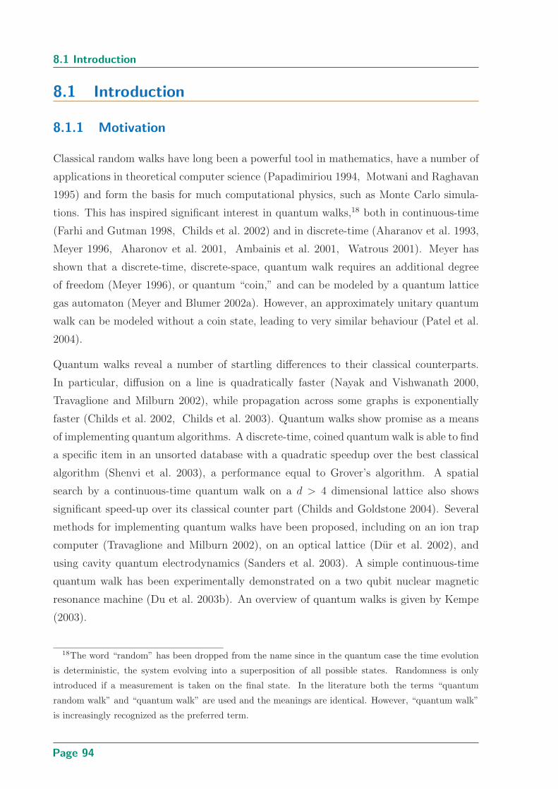
8.1 Introduction
8.1 Introduction
8.1.1 Motivation
Classical random walks have long been a powerful tool in mathematics, have a number of
applications in theoretical computer science (Papadimiriou 1994, Motwani and Raghavan
1995) and form the basis for much computational physics, such as Monte Carlo simula-
tions. This has inspired significant interest in quantum walks,18 both in continuous-time
(Farhi and Gutman 1998, Childs et al. 2002) and in discrete-time (Aharanov et al. 1993,
Meyer 1996, Aharonov et al. 2001, Ambainis et al. 2001, Watrous 2001). Meyer has
shown that a discrete-time, discrete-space, quantum walk requires an additional degree
of freedom (Meyer 1996), or quantum “coin,” and can be modeled by a quantum lattice
gas automaton (Meyer and Blumer 2002a). However, an approximately unitary quantum
walk can be modeled without a coin state, leading to very similar behaviour (Patel et al.
2004).
Quantum walks reveal a number of startling differences to their classical counterparts.
In particular, diffusion on a line is quadratically faster (Nayak and Vishwanath 2000,
Travaglione and Milburn 2002), while propagation across some graphs is exponentially
faster (Childs et al. 2002, Childs et al. 2003). Quantum walks show promise as a means
of implementing quantum algorithms. A discrete-time, coined quantum walk is able to find
a specific item in an unsorted database with a quadratic speedup over the best classical
algorithm (Shenvi et al. 2003), a performance equal to Grover’s algorithm. A spatial
search by a continuous-time quantum walk on a d > 4 dimensional lattice also shows
significant speed-up over its classical counter part (Childs and Goldstone 2004). Several
methods for implementing quantum walks have been proposed, including on an ion trap
computer (Travaglione and Milburn 2002), on an optical lattice (Dur et al. 2002), and
using cavity quantum electrodynamics (Sanders et al. 2003). A simple continuous-time
quantum walk has been experimentally demonstrated on a two qubit nuclear magnetic
resonance machine (Du et al. 2003b). An overview of quantum walks is given by Kempe
(2003).
18The word “random” has been dropped from the name since in the quantum case the time evolution
is deterministic, the system evolving into a superposition of all possible states. Randomness is only
introduced if a measurement is taken on the final state. In the literature both the terms “quantum
random walk” and “quantum walk” are used and the meanings are identical. However, “quantum walk”
is increasingly recognized as the preferred term.
Page 94
Chapter 8 Quantum Walks with History Dependence
8.1.2 Single coin quantum walk
A direct translation of a classical discrete random walk into the quantum domain is not
possible. If a quantum particle moving in one-dimension along a line is updated at each
step, in superposition, to the left and right, the global process is necessarily non-unitary.
However, the addition of a second degree of freedom, the chirality, taking values L and R,
allows interesting quantum walks to be constructed. Consider a particle whose position is
discretized in one-dimension. Let HP be the Hilbert space of particle positions, spanned
by the basis |x〉 : x ∈ Z. In each time-step the particle will move either to the left or
right depending on its chirality. Let HC be the Hilbert space of chirality, or “coin” states,
spanned by the orthonormal basis |L〉, |R〉. A simple quantum walk in the Hilbert space
HP⊗HC consists of a quantum mechanical “coin toss,” a unitary operation U on the coin
state, followed by the updating of the position to the left or right:
E = (S ⊗ PR + S−1 ⊗ PL)(IP ⊗ U), (8.1)
where S is the shift operator in position space, S|x〉 = |x+1〉, IP is the identity operator in
position space, and PR and PL are projection operators on the coin space with PR + PL =
IC, the coin identity operator. For example, a walk controlled by an unbiased quantum
coin is carried out by the transformations
|x, L〉 → 1√2
(|x − 1, L〉 + i|x + 1, R〉) ,
|x,R〉 → 1√2
(i|x − 1, L〉 + |x + 1, R〉) .(8.2)
Figure 8.1 shows the distribution of probability density after 100 steps of Eq. (8.2) with
the initial state |ψ0〉 = (|0, L〉 − |0, R〉)/√
2 . Notice that the scheme of Eq. (8.2) is
equivalent to the Hadamard quantum walk with initial state (|0, L〉 + i|0, R〉)/√
2. The
initial state |ψ0〉 is chosen so that a symmetrical distribution results. In fact the states
|0, R〉 and |0, L〉 evolve independently. This can be seen since any flip |R〉 ↔ |L〉 involves
multiplication by a factor of i. Thus, any |x, L〉 state that started from |0, R〉 will be
multiplied by an odd power of i and is orthogonal to any |x, L〉 state that originated from
|0, L〉, and similarly for the |x,R〉 states. Figure 8.1 contrasts sharply with a classical
coined random walk, which gives rise to a Gaussian distribution spreading in proportion
to√
t.
Page 95
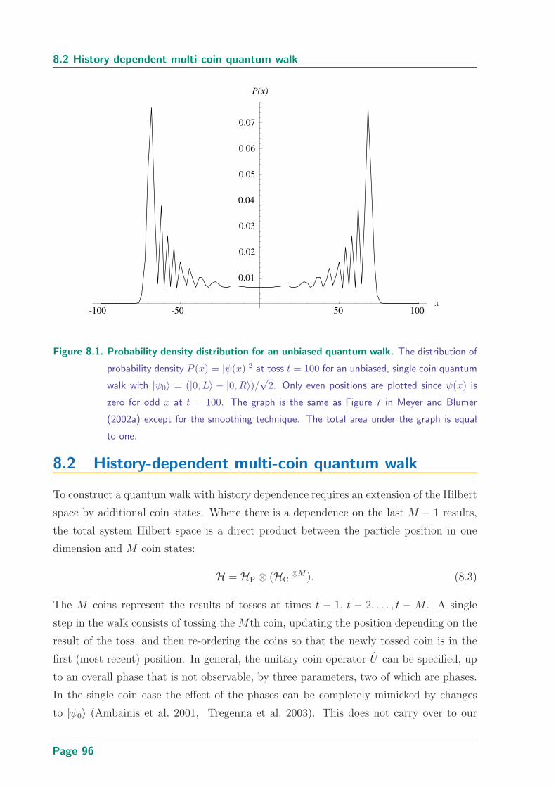
8.2 History-dependent multi-coin quantum walk
-100 -50 50 100x
0.01
0.02
0.03
0.04
0.05
0.06
0.07
P(x)
Figure 8.1. Probability density distribution for an unbiased quantum walk. The distribution of
probability density P (x) = |ψ(x)|2 at toss t = 100 for an unbiased, single coin quantum
walk with |ψ0〉 = (|0, L〉 − |0, R〉)/√
2. Only even positions are plotted since ψ(x) is
zero for odd x at t = 100. The graph is the same as Figure 7 in Meyer and Blumer
(2002a) except for the smoothing technique. The total area under the graph is equal
to one.
8.2 History-dependent multi-coin quantum walk
To construct a quantum walk with history dependence requires an extension of the Hilbert
space by additional coin states. Where there is a dependence on the last M − 1 results,
the total system Hilbert space is a direct product between the particle position in one
dimension and M coin states:
H = HP ⊗ (HC⊗M). (8.3)
The M coins represent the results of tosses at times t − 1, t − 2, . . . , t − M . A single
step in the walk consists of tossing the Mth coin, updating the position depending on the
result of the toss, and then re-ordering the coins so that the newly tossed coin is in the
first (most recent) position. In general, the unitary coin operator U can be specified, up
to an overall phase that is not observable, by three parameters, two of which are phases.
In the single coin case the effect of the phases can be completely mimicked by changes
to |ψ0〉 (Ambainis et al. 2001, Tregenna et al. 2003). This does not carry over to our
Page 96

Chapter 8 Quantum Walks with History Dependence
multi-coin history-dependent scheme. However, for the sake of simplicity the phases shall
be omitted, giving
U(ρ) =
( √ρ i
√1 − ρ
i√
1 − ρ√
ρ
)
, (8.4)
where 1 − ρ is the classical probability that the coin changes state, with ρ = 12
being an
unbiased coin. To allow for history dependence, ρ will depend upon the results of the last
M − 1 coin tosses, so that a single step is effected by the operator
E =(
S ⊗ IC⊗(M−1) ⊗ PR + S−1 ⊗ IC
⊗(M−1) ⊗ PL
)
×
IP ⊗∑
j1,...,jM−1∈L,RP∗
j1...jM−1⊗ U(ρj1...jM−1
)
,(8.5)
where Pj, j ∈ L,R is the projection operator of the Mth coin onto the state |j〉and P∗
j1...jM−1, jk ∈ L,R is the projection operator of the first M − 1 coins onto the
state |j1 . . . jM−1〉. The second parenthesized term in Eq. (8.5) flips the Mth coin with
a parameter ρ that depends upon the state of the first M − 1 coins, while the first term
updates the particle position depending on the result of the flip. Re-ordering of the coins
is then achieved by
O = IP ⊗∑
j1,...,jM∈L,R|jM j1 . . . jM−1〉〈j1 . . . jM−1 jM |. (8.6)
This scheme is distinct from that of Brun et al. (2003b) on quantum walks with multiple
coins, where the walk is carried out by cycling through a given sequence of M coins,
U(ρ1), . . . , U(ρM). In Brun’s scheme, a coin toss is performed by
E = (S ⊗ IC⊗(M−1) ⊗ PR + S−1 ⊗ IC
⊗(M−1) ⊗ PL)(
IP ⊗ IC⊗(M−1) ⊗ U(ρk)
)
, (8.7)
where k = (t mod M), and the step is completed by the O operator as before. The scheme
has memory but not the dependence on history of the current method. The two schemes
are only equivalent when all the ρk and ρj1...jM−1are equal, for example, when all the coins
are unbiased. This amounts to asserting that the scheme of Brun et al. (2003b) does not
display Parrondian behaviour.
The probability density distributions for unbiased 2, 3, and 4 coin history-dependent
quantum walks, with initial states that are an equal superposition of the possible L ↔ R
antisymmetric coin states19 are shown in Figure 8.2. These distributions are essentially
symmetric versions of the graphs of Brun et al. (2003b) that result from an initial state
|ψ0〉 = |R〉⊗M .
19For example, with M = 2, the initial state is |ψ0〉 = (|0, LL〉− |0, LR〉− |0, RL〉+ |0, LL〉)/2. For the
purposes of this thesis an initial state that is symmetrical for L ↔ R could equally well have been chosen.
Page 97

8.3 Results and discussion
-100 -50 50 100x
0.02
0.04
0.06
0.08
0.1
0.12
0.14
P(x)
M
M
M
=2
=3
=4
Figure 8.2. Probability density distributions for 2-, 3- and 4-coin unbiased quantum walks.
The probability density distributions P (x) = |ψ(x)|2 at toss t = 100, for the 2- (red), 3-
(green) and 4- (blue) coin unbiased, symmetrical, quantum walks. Only even positions
are plotted since ψ(x) is zero for odd x at t = 100. The area under each curve is equal
to one.
8.3 Results and discussion
For arbitrary M we have, as for the M = 1 case, two parts of the initial state that evolve
without interacting. Thus, for M = 2 for example, states arising from |0, LL〉 and |0, RR〉will interfere, as will states arising from |0, LR〉 and |0, RL〉, but the two groups evolve
into states that are orthogonal, for any given x. For the M coin quantum walk there are
M + 1 peaks with even values of M having a central peak, the others necessarily being
symmetrically placed around x = 0 by our choice of initial state. The outer most pair of
peaks are in the same position as the peaks for M = 1 (Figure 8.1) at x(t) ≈ 0.68t. All
the peaks are interference phenomenon, the central one being the easiest to understand.
It arises since there are states centred on x = 0 that cycle back to themselves (i.e., that
are stationary states over a certain time period). With M = 2, the simplest cycle over
However, the antisymmetric starting state is the one that gives the correct behaviour in the presence of
a potential. The state |ψ0〉 is the quantum equivalent of the average over past histories that is taken in
the classical history-dependent Parrondo game.
Page 98

Chapter 8 Quantum Walks with History Dependence
t = 2 is proportional to
(|0, LR〉 − |0, RL〉)/√
2 → (| +1, RL〉 + i| −1, LL〉 − | −1, LR〉 − i| +1, RR〉)/2→ (|0, LR〉 − |0, RL〉)/
√2.
(8.8)
At the second step, complete destructive interference occurs for the states with x = ±2,
so that there is no probability flux leaving the central three x values. In practice, the
central region asymptotically approaches a more complex stationary cycle than Eq. (8.8),
such as the t = 2 cycle
|ψcentre〉 ∝ (ai − b)(| − 2, LL〉 + | + 2, RR〉)+ (1 − a − i + bi)(| − 2, LR〉 + | + 2, RL〉)+ (i − 1)(| − 2, RL〉 + | + 2, LR〉)+ (b − ai)(|0, LL〉 + |0, RR〉) + (a + bi)(|0, LR〉 + |0, RL〉),
(8.9)
where a and b are real.
Adjusting the values of the various ρ can introduce a bias into the walk. To create a
quantum walk analogous to the history-dependent game B of Sec. 7.2.2 requires M = 3,
giving four parameters, ρRR, ρRL, ρLR and ρLL. Figure 8.3 shows the affect of individual
variations in these parameters on the expectation value and standard deviation of the
position after 100 time-steps. Some examples of the probability density distribution for
biased 3-coin quantum walks are given in Figure 8.4. As ρRR increases, the right-most
peak moves further towards positive x as a consequence of the increased probability of
consecutive R results. The behaviour resulting from changes in ρRL is more complex. The
effect of variations in ρLL or ρLR is the mirror image of that for ρRR or ρRL, respectively.
8.4 Quantum Parrondo effect
It is useful to consider the classical limit to our quantum scheme. That is, the random
walk that would result if the scattering amplitudes were replaced by classical probabilities.
As an example consider the M = 2 case, with winning probabilities 1 − ρL and 1 − ρR.
The analysis below follows that of Parrondo et al. (2000). Markov chain methods cannot
be used directly because of the history dependence of the scheme. If, however, the vector
y(t) = [x(t − 1) − x(t − 2), x(t) − x(t − 1)] (8.10)
Page 99

8.4 Quantum Parrondo effect
0.2 0.4 0.6 0.8 1.0ρ
-8
-6
-4
-2
2
4
<x>
RR
RL
0.2 0.4 0.6 0.8 1.0ρ
30
35
40
45
xσ
RR
RL
Figure 8.3. Expectation value and standard deviation of position for a 3-coin quantum walk
for various parameter values. For the M = 3 quantum history-dependent walk, 〈x〉and σx at time-step t = 100 as a function of ρRR (solid line) or ρRL (dashed line) while
the other ρij are kept constant at 12 . Varying ρLL has the opposite effect on 〈x〉 and
the same on σx as varying ρRR. Similarly for ρLR compared to ρRL
(a)
-100 -50 50 100x
0.05
0.10
P(x)
(b)
-100 -50 50 100x
0.05
0.10
P(x)
Figure 8.4. Probability density distribution for biased 3-coin quantum walks. The probability
density distributions P (x) = |ψ(x)|2 at toss t = 100, for biases (a) ρRR = 0.4 (blue)
and 0.6 (red), and (b) ρRL = 0.3 (blue) and 0.7 (red), with all the other ρij = 0.5. The
unbiased distribution is shown in green in both figures. The distributions for biases in
ρLL and ρLR are reflections about x = 0 of those for ρRR and ρRL, respectively. Only
even positions are plotted since ψ(x) is zero for odd x at t = 100. The area under each
curve is equal to one.
Page 100
Chapter 8 Quantum Walks with History Dependence
is formed, where x(t) is the position at time t, then y(t) forms a discrete-time Markov chain
between the states [−1,−1], [−1, +1], [+1,−1] and [+1, +1] with a transition matrix
T =
ρL 1 − ρL 0 0
0 0 ρR 1 − ρR
1 − ρL ρL 0 0
0 0 1 − ρR ρR
. (8.11)
Define πij(t) to be the probability of y(t) = [i, j], i, j ∈ −1, +1. A state is now
transformed by Tπ at each time-step. Having represented the history-dependent game
as a discrete-time Markov chain, the standard Markov techniques can be applied. The
equilibrium distribution is found by solving Tπs = πs. This yields πs = [1, 1, 1, 1]/4,
giving a process with no net bias to the left or right irrespective of the values of ρL
and ρR. The same analysis holds for M > 2. The probability density distributions are
approximately Gaussian, centred on zero. However, interference in the quantum case
presents an entirely different picture.
The comparison with the classical history-dependent Parrondo game requires M = 3. For
game A, we select the unbiased game, ρLL = ρLR = ρRL = ρRR = 0.5. For game B, we
choose, for example, ρRR = 0.55 or ρLR = 0.6 to produce a suitable bias (see Figure 8.3).
The operators associated with A and B are applied repeatedly, in some fixed sequence, to
the state |ψ〉. For example, the results of the game sequence AABB after t time-steps is
|ψt〉 = (BBAA)t/4|ψ0〉, (8.12)
where t is a multiple of four. Figure 8.5 displays 〈x〉 for various sequences. Of sequences
up to length four, with game B biased by ρRR > 0.5 only AABB and AAB give a positive
expectation, while when game B is biased by ρLR > 0.5 only AAAB is positive. These
results hold for ρ up to approximately 0.6, above which there are no positive sequences
of length less than or equal to four.
The sequences AABB and BBAA can be considered the same but with different initial
states. That is, if instead of |ψ0〉, we start with |ψ′0〉 = AA|ψ0〉, BBAA gives the same
results (displaced by two time-steps) as AABB does with the original starting state. In
the classical case, altering the order of the sequence results in the same trend but with a
small offset, as one might expect. However, as Figure 8.5 indicates, the change of order in
the quantum case can produce radically different results. This feature also appears in the
quantum Parrondo model of Meyer and Blumer (2002a)—recall their model is based on
a position-dependent scheme rather than a history-dependent one as in the present case.
Details of their scheme are given in Chapter 7.
Page 101
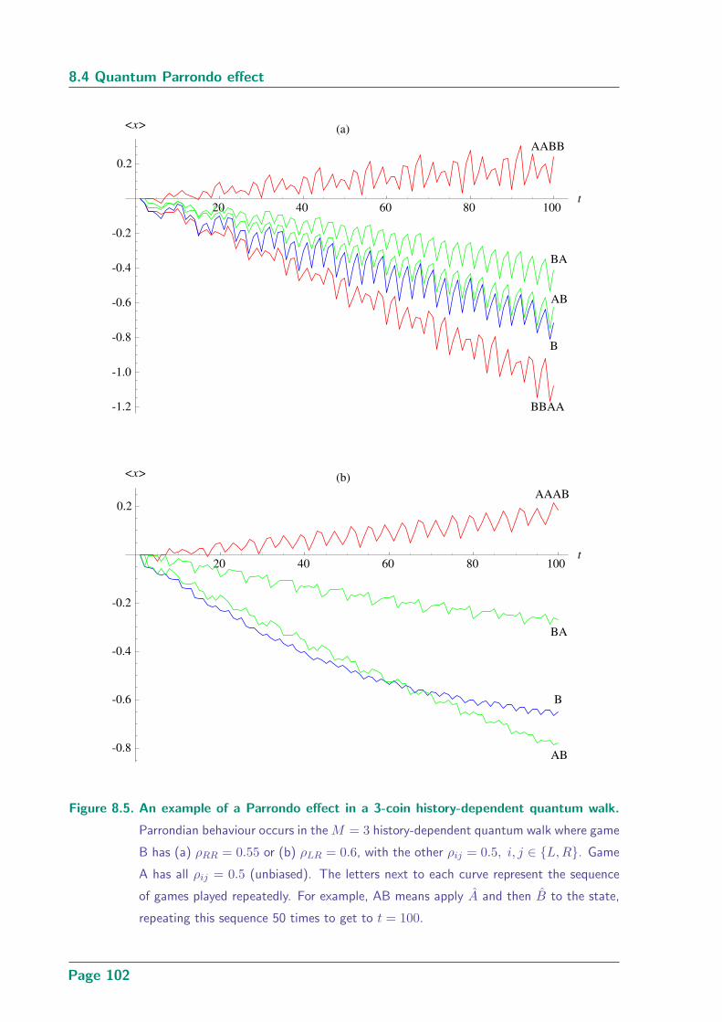
8.4 Quantum Parrondo effect
20 40 60 80 100t
-1.2
-1.0
-0.8
-0.6
-0.4
-0.2
0.2
<x> (a)
B
AB
BA
AABB
BBAA
20 40 60 80 100t
-0.8
-0.6
-0.4
-0.2
0.2
<x> (b)
B
AB
BA
AAAB
Figure 8.5. An example of a Parrondo effect in a 3-coin history-dependent quantum walk.
Parrondian behaviour occurs in the M = 3 history-dependent quantum walk where game
B has (a) ρRR = 0.55 or (b) ρLR = 0.6, with the other ρij = 0.5, i, j ∈ L, R. Game
A has all ρij = 0.5 (unbiased). The letters next to each curve represent the sequence
of games played repeatedly. For example, AB means apply A and then B to the state,
repeating this sequence 50 times to get to t = 100.
Page 102

Chapter 8 Quantum Walks with History Dependence
8.5 Summary
A scheme for a discrete-time quantum walk with history dependence has been presented,
involving the use of multiple quantum coins. By suitable selection of the amplitudes
for coin flips dependent on certain histories, the walk can be biased to give positive or
negative 〈x〉. In common with many other properties of quantum walks, the bias results
from interference, since the classical equivalent of our walks are unbiased. With a starting
state averaged over possible histories, the average spread of probability density in the
multi-coin scheme is slower than in the single coin case, with the appearance of multiple
peaks in the distribution. For even numbers of coins there is a substantial probability of
x ≈ 0. However, the positions of the outer most peaks are the same as those of a single
coin quantum walk. As the memory effect increases, the dispersion of the quantum walk
decreases. One may speculate that this feature may be relevant to an understanding of
decoherence, here considered as loss of coherence within the central portion of the graph
around x ≈ 0. In particular, the dispersion in the wavefunction decreases as we move
from a first-order Markov system to a non-first-order Markov system, that is, one with
memory. This is consistent with the idea that the Markovian approximations tend to
over-estimate the decoherence of the system (Blum 1981). Indeed, the form of a classical
distribution is quickly approached as the quantum coins decohere (Brun et al. 2003a).
The scheme presented in this chapter is a quantum analog of the history-dependent game
in the form of Parrondo’s paradox presented in Sec. 7.2.2. The quantum history-dependent
walk also exhibits a Parrondo effect, where the disruption of the history dependence in a
biased walk by mixing with a second, unbiased walk can reverse the bias. In distinction to
the classical case, the effect seen here is very sensitive to the exact sequence of operations, a
quality it shares with other forms of quantum Parrondo’s games, as discussed in Sec. 7.3.1.
This sensitivity is consistent with the idea that the effect relies on full coherence over space
and in time.
Only quantum walks on a line have been considered. The effect of memory driven quantum
walks on networks with different topologies and whether the memory structure can be
chosen to optimize the path in such networks, are fascinating open questions.
Page 103
Page 104
Chapter 9
Some Ideas on QuantumCellular Automata
CELLULAR automata provide a means of obtaining complex be-
haviour from a simple array of cells and a deterministic updating
rule. They supply a method of computation that dispenses with
the need for manipulation of individual cells. Classical cellular automata have
proved of great interest to computer scientists but the construction of quan-
tum cellular automata pose particular difficulties. This chapter is a brief
introduction to quantum cellular automata and presents a version of John
Conway’s famous two-dimensional classical cellular automata Life that has
some quantum-like features, including interference effects. Some basic struc-
tures in the new automata are given and comparisons are made with Conway’s
game of Life.
Page 105

9.1 Background and motivation
9.1 Background and motivation
9.1.1 Classical cellular automata
A cellular automaton (CA) consists of an infinite array of identical cells, the states of
which are simultaneously updated in discrete time steps according to a deterministic rule.
Formally, they consist of a quadruple (d,Q,N, f), where d ∈ Z+ is the dimensionality of
the array, Q is a finite set of possible states for a cell, N ⊂ Zd is a finite neighbourhood,
and f : Q|N | → Q is a local mapping that specifies the transition rule of the automaton.
The simplest cellular automata are constructed from a one-dimensional array of cells tak-
ing binary values, with a nearest neighbour transition function, as indicated in Figure 9.1.
Such CA were studied intensely by Wolfram (1983) in a publication that lead to a resur-
gence of interest in the field. Wolfram classified cellular automata into four classes. The
classes showed increasingly complex behaviour, culminating in class four automata that
exhibited self-organization, that is, the appearance of order from a random initial state.
In general, information is lost during the evolution of a CA. Knowledge of the state at
a given time is not sufficient to determine the complete history of the system. However,
reversible CA are of particular importance, for example, in the modeling of reversible phe-
nomena. Furthermore, it has been shown that there exists a one-dimensional reversible
CA that is computationally universal (Morita and Harao 1989). Toffoli (1977) demon-
strated that any d-dimensional CA could be simulated by a (d+1)-dimensional reversible
CA and later Morita (1995) found a method using partitioning (see Figure 9.2) where
by any one-dimensional CA can be simulated by a reversible one-dimensional CA. There
is an algorithm for deciding on the reversibility of a one-dimensional CA (Amoroso and
Patt 1972), but in dimensions greater than one, the reversibility of a CA is, in general,
undecidable (Kari 1990).
9.1.2 Conway’s game of Life
John Conway’s game of Life (Gardner 1970) is a well known two-dimensional CA where
cells are arranged in a square grid and have binary values generally known as “dead” or
“alive.” The status of the cells change in discrete time steps known as “generations.” The
new value depends upon the number of living neighbours, the general idea being that a
cell dies if there is either overcrowding or isolation. There are many different rules that
can be applied for birth or survival of a cell and a number of these give rise to interesting
Page 106
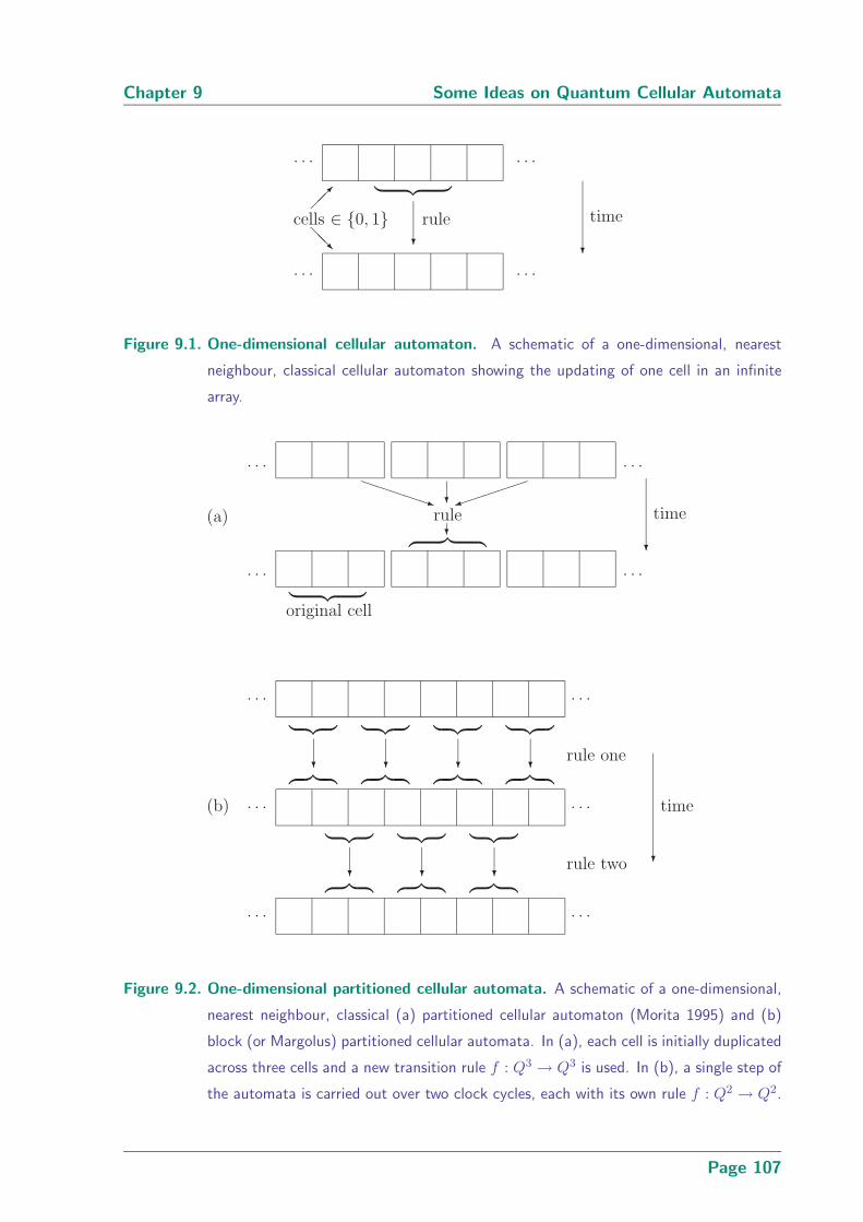
Chapter 9 Some Ideas on Quantum Cellular Automata
. . . . . .
. . . . . .
︸ ︷︷ ︸
?rule
?
time¡¡µ
@@R
cells ∈ 0, 1
Figure 9.1. One-dimensional cellular automaton. A schematic of a one-dimensional, nearest
neighbour, classical cellular automaton showing the updating of one cell in an infinite
array.
. . . . . .
. . . . . .
PPPPPq³³³³³)?
rule?
︷ ︸︸ ︷ ?
time
︸ ︷︷ ︸
original cell
. . . . . .
. . . . . .
. . . . . .
︸ ︷︷ ︸ ︸ ︷︷ ︸ ︸ ︷︷ ︸ ︸ ︷︷ ︸
︷ ︸︸ ︷ ︷ ︸︸ ︷ ︷ ︸︸ ︷ ︷ ︸︸ ︷
︸ ︷︷ ︸ ︸ ︷︷ ︸ ︸ ︷︷ ︸
︷ ︸︸ ︷ ︷ ︸︸ ︷ ︷ ︸︸ ︷
? ? ? ?
? ? ?
rule one
rule two
time
?
(b)
(a)
Figure 9.2. One-dimensional partitioned cellular automata. A schematic of a one-dimensional,
nearest neighbour, classical (a) partitioned cellular automaton (Morita 1995) and (b)
block (or Margolus) partitioned cellular automata. In (a), each cell is initially duplicated
across three cells and a new transition rule f : Q3 → Q3 is used. In (b), a single step of
the automata is carried out over two clock cycles, each with its own rule f : Q2 → Q2.
Page 107
9.1 Background and motivation
properties such as still lives (stable patterns), oscillators (patterns that periodically re-
peat), spaceships or gliders (fixed shapes that move across the Life universe), glider guns,
and so on (Gardner 1971, Gardner 1983, Berlekamp et al. 1982). Conway’s original
rules are one of the few that are balanced between survival and extinction of the Life
“organisms.” In this version a dead (or empty) cell becomes alive if it has exactly three
living neighbours, while an alive cell survives if and only if it has two or three living
neighbours. Much literature on the game of Life and its implications exists and a search
on the world wide web reveals numerous resources. For a discussion on the possibilities
of this and other CA the interested reader is referred to Wolfram (2002).
The simplest still lives and oscillators are given in Figure 9.3, while Figure 9.4 shows a
glider, the simplest and most common moving form. A large enough random collection
of alive and dead cells will, after a period of time, usually decay into a collection of still
lives and oscillators like those shown here, while firing a number of gliders off towards the
outer fringes of the Life universe.
9.1.3 Quantum cellular automata
The idea of generalizing classical cellular automata to the quantum domain was already
considered by Feynman (1982). Grossing and Zeilinger made the first serious attempts to
consider quantum cellular automata (QCA) (Grossing and Zeilinger 1988a, Grossing and
Zeilinger 1988b), though their ideas are considerably different from modern approaches.
Quantum cellular automata are a natural model of quantum computation where the
well developed theory of classical CA might be exploited. Quantum computation using
optical lattices (Mandel et al. 2003) or with arrays of microtraps (Dumke et al. 2002) are
possible candidates for the experimental implementation of useful quantum computing.
It is typical of such systems that the addressing of individual cells is more difficult than
a global change made to the environment of all cells (Benjamin 2000b) and thus they
become natural candidates for the construction of QCA. An accessible discussion of QCA
is provided by Gruska (1999).
The simple idea of quantizing existing classical CA by making the local translation rule
unitary is problematic: the global rule on an infinite array of cells is rarely described by a
well defined unitary operator. One must decide whether a given local unitary rule leads to
“well-formed” unitary QCA (Durr and Santha 2002) that properly transform probabilities
by preserving their sum squared to one. One construction method to achieve the necessary
reversibility of a QCA is to partition the system into blocks of cells and apply blockwise
Page 108

Chapter 9 Some Ideas on Quantum Cellular Automata
¡@ = alive p = empty or dead
¡¡@@
¡¡@@
(i) block
¡
¡
@
@¡ ¡@ @p
(ii) tub
¡
¡
@
@
¡ ¡@ @¡ ¡@ @p
p
(iii) boat
(a) still lives
¡¡¡
@@@p p
initial
¡ ¡ ¡@ @ @pp
1st gen.
¡¡¡
@@@p p
2nd gen.
(b) blinker
¡¡@@ ¡@
¡ ¡@ @¡@p
pppp
ppp
pp
initial
¡¡@@
¡¡@@
¡¡@@
¡¡@@p
ppp
pp
pp
1st gen.
¡¡@@ ¡@
¡ ¡@ @¡@p
pppp
ppp
pp
2nd gen.
(c) beacon
Figure 9.3. Simple patterns in Conway’s Life. A small sample of the simplest structures in
Conway’s Life: (a) the simplest still-lives (stable patterns) and (b)–(c) the simplest
period two oscillators (periodic patterns). A number of these forms will normally evolve
from any moderate sized random collection of alive and dead cells.
unitary transformations. This is the quantum generalization to the scheme shown in
Figure 9.2(b)—indeed, all QCA, even those with local irreversible rules, can be obtained
in such a manner (Schumacher and Werner 2004). Formal rules for the realization of
QCA using a transition rule based on a quasi-local algebra on the lattice sites is described
by Schumacher and Werner (2004). In this formalism, a unitary operator for the time
evolution is not necessary. The authors demonstrate that all nearest neighbour one-
dimensional QCA arise by a combination of a single qubit unitary, a possible left- or
right-shift, and a control-phase gate,20 as indicated in Figure 9.5.
A Mathematica package to implement the scheme of Figure 9.5 is given in Sec. A.4.1.
Reversible one-dimensional nearest neighbour classical CA are a subset of the quantum
ones. In the classical case, the single qubit unitary can only be the identity or a bit-flip,
20A control-phase gate is a two-qubit gate that multiplies the target qubit by(
1 00 exp(iφ)
)if the control
qubit is 1.
Page 109

9.2 Semi-quantum Life
¡@¡@ ¡
¡¡
@@@
pp
pp
p p p pppp
initial
¡
¡
@
@
¡¡@@p
pp
¡@pp
pp
p p p p
1st gen.
¡@¡@
¡ ¡ ¡@ @ @ppp
pp
pp
p p p p
2nd gen.
¡@
¡¡@@ ¡
¡@@
pppp
ppp
pp
p
p
3rd gen.
¡@¡@ ¡
¡¡
@@@
pp
pp
p p p
pppp
4th gen.
Figure 9.4. A Life glider. In Conway’s Life, the simplest spaceship (a pattern that moves continu-
ously through the Life universe), the glider. The figure shows how the glider moves one
cell diagonally over a period of four generations.
U U U U U. . . . . .
HHHH
HHHH
HHHH
HHHHH
φ φ. . . . . .
one qubit unitaries
right shift
control-phase gates?
time
Figure 9.5. One-dimensional quantum cellular automaton. A schematic of a one-dimensional
nearest neighbour quantum cellular automaton according to the scheme of Schumacher
and Werner (2004) (from Figure 10 of that publication). The right-shift may be replaced
by a left-shift or no shift.
while the control-phase gate is absent. This leaves just six classical CA, all of which are
trivial.
9.2 Semi-quantum Life
9.2.1 The idea
Conway’s Life is irreversible while, in the absence of a measurement, quantum mechanics is
reversible. In particular, operators that represent measurable quantities must be unitary.
A full quantum Life on an infinite array would be impossible given the known difficulties
Page 110

Chapter 9 Some Ideas on Quantum Cellular Automata
of constructing unitary QCA (Meyer 1996). Interesting behaviour is still obtained in
a version of Life that has some quantum mechanical features. Cells are representing
by classical sine-wave oscillators with a period equal to one generation, an amplitude
between zero and one, and a variable phase. The amplitude of the oscillation represents
the coefficient of the alive state so that the square of the amplitude gives the probability
of finding the cell in the alive state when a measurement of the “health” of the cell is
taken. If the initial state of the system contains at least one cell that is in a superposition
of eigenstates the neighbouring cells will be influenced according to the coefficients of the
respective eigenstates, propagating the superposition to the surrounding region.
If the coefficients of the superpositions are restricted to positive real numbers, qualitatively
new phenomena are not expected. By allowing the coefficients to be complex, that is, by
allowing phase differences between the oscillators, qualitatively new phenomena such as
interference effects, may arise. The interference effects seen are those due to an array of
classical oscillators with phase shifts and are not fully quantum mechanical.
9.2.2 A first model
To represent the state of a cell introduce the following notation:
|ψ〉 = a|alive〉 + b|dead〉, (9.1)
subject to the normalization condition
|a|2 + |b|2 = 1. (9.2)
The probability of measuring the cell as alive or dead is |a|2 or |b|2, respectively. If the
values of a and b are restricted to non-negative real numbers, destructive interference does
not occur. The model still differs from a classical probabilistic mixture, since here it is the
amplitudes that are added and not the probabilities. In our model |a| is the amplitude of
the oscillator. Restricting a to non-negative real numbers corresponds to the oscillators
all being in phase.
The birth, death and survival operators have the following effects:
B|ψ〉 = |alive〉,D|ψ〉 = |dead〉,S|ψ〉 = |ψ〉.
(9.3)
Page 111
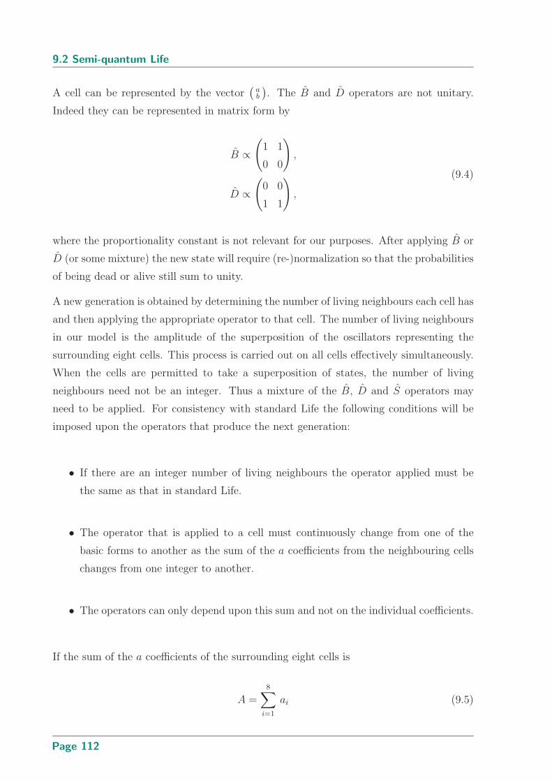
9.2 Semi-quantum Life
A cell can be represented by the vector(
ab
). The B and D operators are not unitary.
Indeed they can be represented in matrix form by
B ∝(
1 1
0 0
)
,
D ∝(
0 0
1 1
)
,
(9.4)
where the proportionality constant is not relevant for our purposes. After applying B or
D (or some mixture) the new state will require (re-)normalization so that the probabilities
of being dead or alive still sum to unity.
A new generation is obtained by determining the number of living neighbours each cell has
and then applying the appropriate operator to that cell. The number of living neighbours
in our model is the amplitude of the superposition of the oscillators representing the
surrounding eight cells. This process is carried out on all cells effectively simultaneously.
When the cells are permitted to take a superposition of states, the number of living
neighbours need not be an integer. Thus a mixture of the B, D and S operators may
need to be applied. For consistency with standard Life the following conditions will be
imposed upon the operators that produce the next generation:
• If there are an integer number of living neighbours the operator applied must be
the same as that in standard Life.
• The operator that is applied to a cell must continuously change from one of the
basic forms to another as the sum of the a coefficients from the neighbouring cells
changes from one integer to another.
• The operators can only depend upon this sum and not on the individual coefficients.
If the sum of the a coefficients of the surrounding eight cells is
A =8∑
i=1
ai (9.5)
Page 112

Chapter 9 Some Ideas on Quantum Cellular Automata
then the following set of operators, depending upon the value of A, is the simplest that
has the required properties
0 ≤ A ≤ 1; G0 = D,
1 < A ≤ 2; G1 = (√
2 + 1)(2 − A)D + (A − 1)S,
2 < A ≤ 3; G2 = (√
2 + 1)(3 − A)S + (A − 2)B,
3 < A < 4; G3 = (√
2 + 1)(4 − A)B + (A − 3)D,
A ≥ 4; G4 = D.
(9.6)
For integer values of A, the G operators are the same as the basic operators of standard
Life, as required. For non-integer values in the range (1, 4), the operators are a linear
combination of the standard operators. The factors of√
2 + 1 have been inserted to give
more appropriate behaviour in the middle of each range. For example, consider the case
where A = 3 + 1/√
2, a value that may represent three neighbouring cells that are alive
and one the has a probability of one-half of being alive. The operator in this case is
G =1√2
B +1√2
D ∝ 1√2
(
1 1
1 1
)
. (9.7)
Applying this to either a cell in the alive,(
10
)or dead,
(01
)states will produce the state
|ψ〉 =1√2|alive〉 +
1√2|dead〉 (9.8)
which represents a cell with a 50% probability of being alive. That is, G is an equal combi-
nation of the birth and death operators, as might have been expected given the possibility
that A represents an equal probability of three or four living neighbours. Of course the
same value of A may have been obtained by other combinations of neighbours that do
not lie half way between three and four living neighbours, but one of our requirements is
that the operators can only depend on the sum of the a coefficients of the neighbouring
cells and not on how the sum was obtained.
In general the new state of a cell is obtained by calculating A, applying the appropriate
operator G:(
a′
b′
)
= G
(
a
b
)
, (9.9)
and then normalizing the resulting state so that |a′|2 + |b′|2 = 1. It is this process
of normalization that means that multiplying the operator by a constant has no effect.
Hence, for example, G2 for A = 3 has the same effect as G3 in the limit as A → 3, despite
differing by the constant factor (√
2 + 1).
Page 113
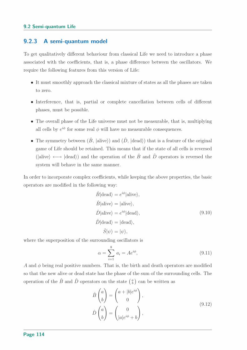
9.2 Semi-quantum Life
9.2.3 A semi-quantum model
To get qualitatively different behaviour from classical Life we need to introduce a phase
associated with the coefficients, that is, a phase difference between the oscillators. We
require the following features from this version of Life:
• It must smoothly approach the classical mixture of states as all the phases are taken
to zero.
• Interference, that is, partial or complete cancellation between cells of different
phases, must be possible.
• The overall phase of the Life universe must not be measurable, that is, multiplying
all cells by eiφ for some real φ will have no measurable consequences.
• The symmetry between (B, |alive〉) and (D, |dead〉) that is a feature of the original
game of Life should be retained. This means that if the state of all cells is reversed
(|alive〉 ←→ |dead〉) and the operation of the B and D operators is reversed the
system will behave in the same manner.
In order to incorporate complex coefficients, while keeping the above properties, the basic
operators are modified in the following way:
B|dead〉 = eiφ|alive〉,B|alive〉 = |alive〉,D|alive〉 = eiφ|dead〉,D|dead〉 = |dead〉,
S|ψ〉 = |ψ〉,
(9.10)
where the superposition of the surrounding oscillators is
α =8∑
i=1
ai = Aeiφ, (9.11)
A and φ being real positive numbers. That is, the birth and death operators are modified
so that the new alive or dead state has the phase of the sum of the surrounding cells. The
operation of the B and D operators on the state(
ab
)can be written as
B
(
a
b
)
=
(
a + |b|eiφ
0
)
,
D
(
a
b
)
=
(
0
|a|eiφ + b
)
,
(9.12)
Page 114

Chapter 9 Some Ideas on Quantum Cellular Automata
with S leaving the cell unchanged. The modulus of the sum of the neighbouring cells A
determines which operators apply, in the same way as before [see Eq. (9.6)]. The addition
of the phase factors for the cells allows for interference effects since the coefficients of alive
cells may not always reinforce in taking the sum, α =∑
ai. A cell with a = −1 still has a
unit probability of being measured in the alive state but its effect on the sum will cancel
that of a cell with a = 1. A phase for the dead cell is retained in order to maintain the
alive ←→ dead symmetry, however, it has no effect. Such an effect would conflict with
the physical model presented earlier and would be inconsistent with Conway’s Life, where
the empty cells have no influence.
A useful notation to represent semi-quantum Life is to use an arrow whose length repre-
sents the amplitude of the a coefficient and whose angle with the horizontal is a measure of
the phase of a. That is, the arrow represents the phaser of the oscillator at the beginning
of the generation. For example
−→ =
(
1
0
)
,
↑ = eiπ/2
(
1/2√
3/2
)
=
(
i/2
i√
3/2
)
,
ր = eiπ/4
(
1/√
2
1/√
2
)
=
(
(1 + i)/2
(1 + i)/2
)
,
(9.13)
etc. In this picture α is the vector sum of the arrows. This notation includes no infor-
mation about the b coefficient. The magnitude of this coefficient can be determined from
a and the normalization condition. The phase of the b coefficient has no effect on the
evolution of the game state so it is not necessary to represent this.
9.2.4 Discussion
The above rules have been implemented in the computer algebra language Maple (see
Sec. A.4.2). All the structures of standard Life can be recreated by making the phase
of all the alive cells equal. The interest lies in whether there are new effects in the
semi-quantum model or whether existing effects can be reproduced in simpler or more
generalized structures. The most important aspect not present in standard Life is inter-
ference. Two live cells can work against each other as indicated in Figure 9.6 that shows
an elementary example in a block still life with one cell out of phase with its neighbours. In
standard Life there are linear structures called wicks that die or “burn” at a constant rate.
Page 115

9.3 Summary
The simplest such structure is a diagonal line of live cells as indicated in Figure 9.7(a).
In this, it is not possible to stabilize an end without introducing other effects. In the new
model a line of cells of alternating phase (. . . −→←− . . .) is a generalization of this effect
since it can be in any orientation and the ends can be stabilized easily. Figure 9.7(b)–(c)
shows some examples. A line of alternating phase live cells can be used to create other
structures such as the loop in Figure 9.8. This is a generalization of the boat still life,
Figure 9.3(a)(iii), in the standard model that is of a fixed size and shape. The stability of
the line of −→←−’s results from the fact that while each cell in the line has exactly two
living neighbours, the cells above or below this line have a net of zero (or one at a corner)
living neighbours due to the canceling effect of the opposite phases. No new births around
the line will occur, unlike the case where all the cells are in phase.
Oscillators (Figure 9.3) and spaceships (Figure 9.4) cannot be made simpler than the
minimal examples presented for standard Life. Figure 9.9 shows a stable boundary that
results from the appropriate adjustment of the phase differences between the cells. The
angles have been chosen so that each cell in the line has between two and three living
neighbours, while the empty cells above and below the line have either two or four living
neighbours and so remain life-less. Such boundaries are known in standard Life but require
a more complex structure.
In Conway’s Life interesting effects can be obtained by colliding gliders. In the semi-
quantum model additional effects can be obtained from colliding gliders and “anti-gliders,”
where all the cells have a phase difference of π with those of the original glider. For exam-
ple, a head-on collision between a glider and an anti-glider, as indicated in Figure 9.10,
causes annihilation, where as the same collision between two gliders leaves a block. How-
ever, there is no consistency with this effect since other glider-antiglider collisions produce
alternative effects, sometimes being the same as those from the collision of two gliders.
9.3 Summary
John Conway’s game of Life is a two-dimensional cellular automaton where the new state
of a cell is determined by the sum of neighbouring states that are in one particular state
generally referred to as “alive.” A modification to this model is proposed where the cells
may be in a superposition of the alive and dead states with the coefficient of the alive
state being represented by an oscillator having a phase and amplitude. The equivalent
of evaluating the number of living neighbours of a cell is to take the superposition of the
Page 116
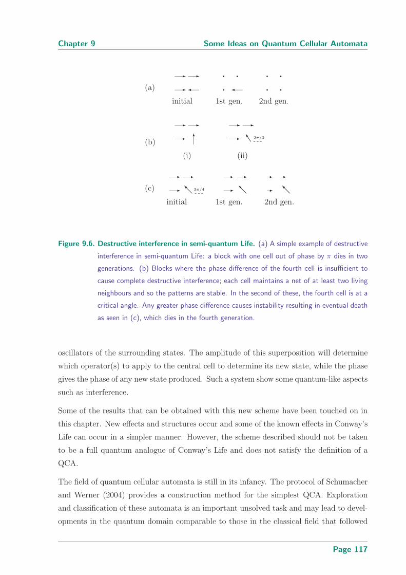
Chapter 9 Some Ideas on Quantum Cellular Automata
- ¾
- -
initial
(a) ¾qq q
1st gen.
2nd gen.
- 6
- -
(i)
(b)- JJ]
- -
2π/3
(ii)
- @@I
- -
3π/4
initial
(c) - @@I
- -
1st gen.
- @@I
- -
2nd gen.
Figure 9.6. Destructive interference in semi-quantum Life. (a) A simple example of destructive
interference in semi-quantum Life: a block with one cell out of phase by π dies in two
generations. (b) Blocks where the phase difference of the fourth cell is insufficient to
cause complete destructive interference; each cell maintains a net of at least two living
neighbours and so the patterns are stable. In the second of these, the fourth cell is at a
critical angle. Any greater phase difference causes instability resulting in eventual death
as seen in (c), which dies in the fourth generation.
oscillators of the surrounding states. The amplitude of this superposition will determine
which operator(s) to apply to the central cell to determine its new state, while the phase
gives the phase of any new state produced. Such a system show some quantum-like aspects
such as interference.
Some of the results that can be obtained with this new scheme have been touched on in
this chapter. New effects and structures occur and some of the known effects in Conway’s
Life can occur in a simpler manner. However, the scheme described should not be taken
to be a full quantum analogue of Conway’s Life and does not satisfy the definition of a
QCA.
The field of quantum cellular automata is still in its infancy. The protocol of Schumacher
and Werner (2004) provides a construction method for the simplest QCA. Exploration
and classification of these automata is an important unsolved task and may lead to devel-
opments in the quantum domain comparable to those in the classical field that followed
Page 117
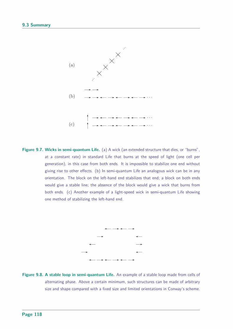
9.3 Summary
(a)
¡¡¡¡
¡¡¡¡
@@
@@
@@
@@
p p p
p p p
(b) - -
- -
¾ ¾ ¾- - - . . .
(c) 6
6
¾ ¾ ¾
¾ ¾ ¾
- - - -
- - - -
. . .
. . .
Figure 9.7. Wicks in semi-quantum Life. (a) A wick (an extended structure that dies, or “burns”,
at a constant rate) in standard Life that burns at the speed of light (one cell per
generation), in this case from both ends. It is impossible to stabilize one end without
giving rise to other effects. (b) In semi-quantum Life an analogous wick can be in any
orientation. The block on the left-hand end stabilizes that end; a block on both ends
would give a stable line; the absence of the block would give a wick that burns from
both ends. (c) Another example of a light-speed wick in semi-quantum Life showing
one method of stabilizing the left-hand end.
¾ ¾ ¾- - -
¾ ¾- -
¾
¾
-
-
-
¾
Figure 9.8. A stable loop in semi-quantum Life. An example of a stable loop made from cells of
alternating phase. Above a certain minimum, such structures can be made of arbitrary
size and shape compared with a fixed size and limited orientations in Conway’s scheme.
Page 118

Chapter 9 Some Ideas on Quantum Cellular Automata
- - - - - - -
JJ] JJ]À
Á ÁJJ. . .. . .
Figure 9.9. A stable boundary in semi-quantum Life. A boundary utilizing appropriate phase
differences to produce stability. The upper cells are out of phase by ±π/3 and the lower
by ±2π/3 with the central line.
-
-
-
-
-
¾
¾
¾
¾
¾
Figure 9.10. A collision between a glider and an anti-glider in semi-quantum Life. A head on
collision between a glider and its phase reversed counter part, an anti-glider, produces
annihilation in six generations.
the exploration of classical CA. Quantum cellular automata are a viable candidate for
achieving useful quantum computing.
Page 119

Page 120

Chapter 10
Conclusions and FutureDirections
Q UANTUM game theory is an exciting new tool for the study
of conflict or competition situations in the quantum domain.
The theory contributes to our understanding of quantum infor-
mation and has the potential for application in quantum con-
trol, quantum algorithms, quantum communication, and other quantum com-
puting tasks. Quantum walks and quantum cellular automata present promis-
ing protocols for the implementation of useful quantum computing. This thesis
has presented new ideas in the above fields. The concluding chapter presents
an extended summary of this work, detailing the original contributions, and
indicating possible future directions.
Page 121

10.1 New quantum models of classical games
10.1 New quantum models of classical games
The starting point for quantum game theory are the existing classical game-theoretic
problems. Existing scenarios are translated into the quantum domain by changing classical
probabilities into quantum probability amplitudes, permitting superpositions of classical
strategies and, possibly, by introducing entanglement between the options of different
players. The original problem remains as a subset of the quantum game. By quantizing
a game, the nature of the game is changed and in that sense quantum games do not
address the original problem. Nevertheless, the quantum models demonstrate what can be
achieved when the game’s domain is expanded into the quantum realm. More importantly,
when dealing with problems in quantum computing and quantum communication, where
the information is quantum, the new theory is necessary to deal with competitive or
conflict situations that may arise. In this thesis, new quantizations of two interesting
game-theoretic problems have been presented.
10.1.1 Monty Hall problem—Chapter 3
The Monty Hall problem originated in a TV game show where the competitor has the
task of guessing behind which of three doors the host has hidden a prize. After an initial
selection by the competitor, the host opens a different door showing that the prize is
not behind it. The player is then given the option of switching their selection to the
untouched door or remaining with their initial choice. “Common sense” seems to suggest
that, now the player knows the prize lies behind one of two doors, both options should
yield a 50/50 chance of securing the prize. The counterintuitive idea that lies behind
this simple problem is this: switching doors yields a two-thirds chance of winning, while
retaining the initial choice of door results in a win only one time in three. This can easily
be verified by referring to Table 3.1 but the ease of this observation did not stop the
Monty Hall problem from generating much interest and controversy when it captured the
attention of the public and of mathematicians in the early 1990s (vos Savant 1991).
Three distinct quantizations of the Monty Hall problem have appeared in the literature,
that described in this thesis being the second (Flitney and Abbott 2002c). Those of Li et
al. (2001) and D’Ariano et al. (2002) are briefly described in the introductory paragraphs
of Sec. 3.2. The quantization scheme presented in this thesis is the one that most directly
follows the classical version. There is a quantum particle and three boxes |0〉, |1〉, and
|2〉. The choices of the contestant (Bob) and the host (Alice) are represented by qutrits
Page 122
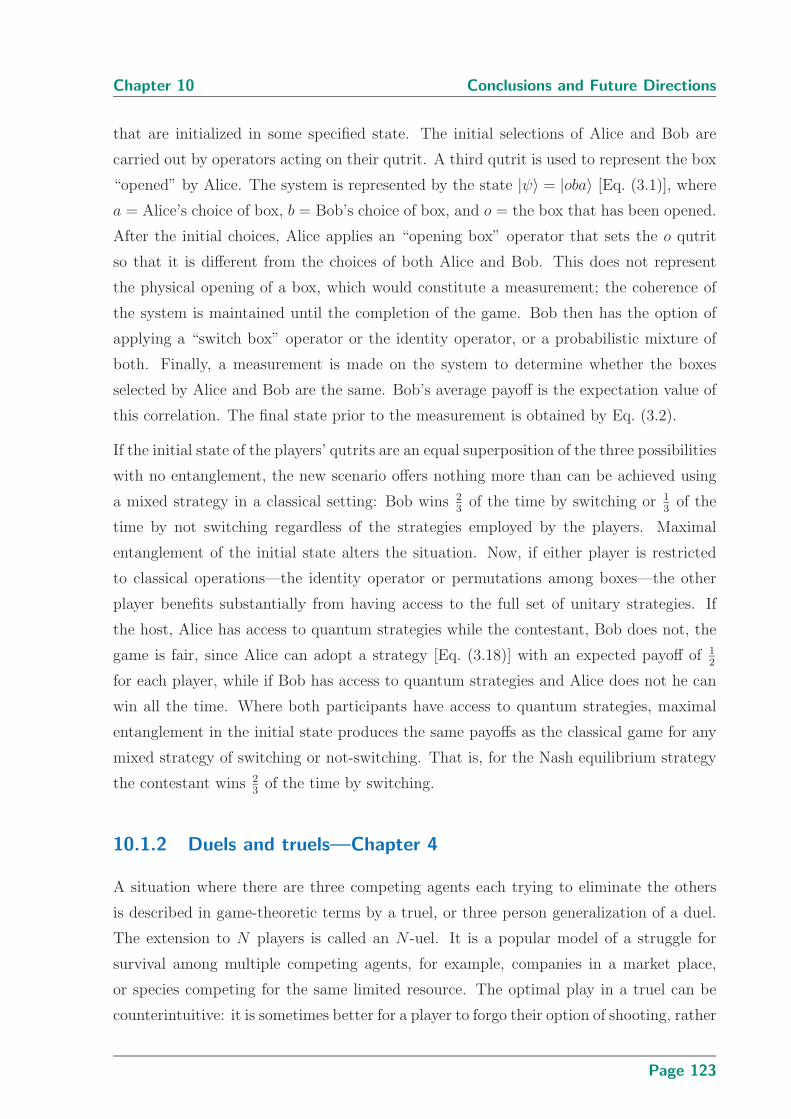
Chapter 10 Conclusions and Future Directions
that are initialized in some specified state. The initial selections of Alice and Bob are
carried out by operators acting on their qutrit. A third qutrit is used to represent the box
“opened” by Alice. The system is represented by the state |ψ〉 = |oba〉 [Eq. (3.1)], where
a = Alice’s choice of box, b = Bob’s choice of box, and o = the box that has been opened.
After the initial choices, Alice applies an “opening box” operator that sets the o qutrit
so that it is different from the choices of both Alice and Bob. This does not represent
the physical opening of a box, which would constitute a measurement; the coherence of
the system is maintained until the completion of the game. Bob then has the option of
applying a “switch box” operator or the identity operator, or a probabilistic mixture of
both. Finally, a measurement is made on the system to determine whether the boxes
selected by Alice and Bob are the same. Bob’s average payoff is the expectation value of
this correlation. The final state prior to the measurement is obtained by Eq. (3.2).
If the initial state of the players’ qutrits are an equal superposition of the three possibilities
with no entanglement, the new scenario offers nothing more than can be achieved using
a mixed strategy in a classical setting: Bob wins 23
of the time by switching or 13
of the
time by not switching regardless of the strategies employed by the players. Maximal
entanglement of the initial state alters the situation. Now, if either player is restricted
to classical operations—the identity operator or permutations among boxes—the other
player benefits substantially from having access to the full set of unitary strategies. If
the host, Alice has access to quantum strategies while the contestant, Bob does not, the
game is fair, since Alice can adopt a strategy [Eq. (3.18)] with an expected payoff of 12
for each player, while if Bob has access to quantum strategies and Alice does not he can
win all the time. Where both participants have access to quantum strategies, maximal
entanglement in the initial state produces the same payoffs as the classical game for any
mixed strategy of switching or not-switching. That is, for the Nash equilibrium strategy
the contestant wins 23
of the time by switching.
10.1.2 Duels and truels—Chapter 4
A situation where there are three competing agents each trying to eliminate the others
is described in game-theoretic terms by a truel, or three person generalization of a duel.
The extension to N players is called an N -uel. It is a popular model of a struggle for
survival among multiple competing agents, for example, companies in a market place,
or species competing for the same limited resource. The optimal play in a truel can be
counterintuitive: it is sometimes better for a player to forgo their option of shooting, rather
Page 123
10.1 New quantum models of classical games
than risk eliminating an opponent only to become the target for the third player. The
optimal strategy is sensitive to the exact conditions under which the truel is carried out. A
non-technical discussion of classical truels is provided by Kilgour and Brams (1997) with
detailed analysis of the case of simultaneous firing (Kilgour 1972) and sequential firing
(Kilgour 1975) provided by the same author. An introduction to classical truels and an
example of the seemingly paradoxical nature of the optimal play has been presented in
Sec. 4.2.
In this thesis a novel quantization scheme for this problem is presented. Each player has a
qubit designating their state, with the computational basis states |0〉 and |1〉 representing
“dead” and “alive,” respectively. The combined state of the players Alice, Bob, and
Charles is |ψ〉 = |qA qB qC〉 [Eq. (4.5)] with the initial state being |ψi〉 = |111〉. The system
is easily extended to more players by the addition of further qubits. The analogue of firing
at an opponent is an attempt to flip an opponent’s qubit using a unitary operator acting
on |ψ〉. An action can only be carried out if the player is alive, so the appropriate unitaries
are control-rotations, or more generally control-SU(2) operations, where the player’s qubit
is the control and the target’s qubit is the subject of the rotation. Equations (4.6) and
(4.7) represent the actions of Alice firing at Bob in a duel or a truel, respectively. The
game consists of a number of rounds of sequential firing. Coherence of the system is
maintained until the completion of the final round, where upon a measurement in the
computational basis is taken on the final state and payoffs are awarded to the players still
living. The formalism for carrying out quantum duels and truels is detailed in Sec. 4.3
with extensions to the case of N players given in Sec. 4.6.
The game differs from the classical scenario in allowing player states to be a superposition
of alive and dead, in permitting dead players to be bought back to life by having their
qubit flipped from |0〉 → |1〉, and by the fact that the players get no information about
the state of the system in intermediate rounds. This latter fact means that, in contrast
to the classical case, players’ decisions are not contingent on the success or otherwise of
previous actions. A player can select the operators they wish to apply for each round at
the beginning of the game, based on their forward estimates of who will be alive at that
stage, rather than making dynamic choices during the game.
A one round, two player quantum duel offers nothing different from the classical game,
but in longer quantum duels phase terms in the player operators can greatly affect the
expected payoffs (see Figures 4.6 and 4.7). If players have discretion over the value of
their phase factors a maximin choice can in principle be calculated provided the number
Page 124

Chapter 10 Conclusions and Future Directions
of rounds is fixed. If one player has a restricted choice the other has a large advantage.
The unitary nature of the operators means that the probability of flipping a dead state
to an alive state is the same as that for the reverse, so it can be advantageous for a
player to fire in the air rather than target the opponent, something that is never true in
a classical duel, and this can result in an equilibrium where both players forgo targeting
their opponent even if there are further rounds to play (see Figure 4.8).
In a quantum truel, interference effects arise when one player is targeted by the other two,
and can have dramatic consequences, either enhancing or diminishing the probability of
survival of the targeted player compared to the classical case. Such interference effects can
occur as early as the first round. As with the case of quantum duels, equilibria can arise
where it is to the disadvantage of each player to target one of the others. Such equilibria
occur more frequently in the quantum case than in the classical where they depend upon
exceptional circumstances.
The optimal play depends on the marksmanship of the players. Section 4.5.1 summarizes
the optimal play for one and two round truels where the third player is a perfect shot.
The regions of parameter space that correspond to the various preferred strategies of the
first two players differ from those of the classical game (see Figures 4.9–4.11).
The analogy with the classical scenario can be made closer by introducing decoherence in
the form of a measurement in the computational basis with probability p after each move.
In the case of a measurement, players can alter their decisions dependent on the result
of the measurement. As the measurement probability is increased from zero to one there
is a smooth transition from the fully quantum game to the classical one as described in
Sec. 4.7.
10.1.3 Future directions
The time when it was exciting to produce quantizations of abstract game theory problems
is mostly past. Future work in this area needs to demonstrate novel effects, in addition
to the interference phenomena that is expected in the quantum world, or have relevance
to particular practical problems in the areas of quantum computing, quantum control or
quantum communication. Game theory is the natural language for competitive scenarios
such as communication in the presence of an eavesdropper. The important task of applying
quantum game theory to the problems of quantum communication remain to be explored.
Classical game theory is regularly applied to problems in queuing theory. The possibility
Page 125

10.2 Quantum 2 × 2 games
of utilizing quantum game theory to produce a quantum theory of queuing has been
mooted (Pati 2003).
10.2 Quantum 2 × 2 games
10.2.1 A quantum player versus a classical player—Chapter 5
The work by Eisert et al. (1999) was one of the two seminal papers on quantum game the-
ory, detailing a protocol for two player, two strategy quantum games with entanglement.
In this work it was noted that, in the well known game of Prisoners’ Dilemma, if one
player has access to quantum strategies while the other player is restricted to the classi-
cal strategy subset, the quantum player could achieve a considerably greater payoff than
they could have achieved playing classically, where the best that could be hoped for is the
(classical) NE result. By selecting the move dubbed by Eisert as the “miracle” move, the
quantum player can partially direct the result of the game towards their preferred result,
regardless of the classical player’s strategy. Indeed, if the strategy of the classical player
is known the quantum player can exploit the entanglement between the players’ qubits
to create any desired final state.
Du et al. (2001b) generalized the Eisert result to Prisoners’ Dilemma with a variable
payoff matrix. The extent of the quantum advantage is dependent on the degree of
entanglement between the qubits that represent the players’ strategies. Below a certain
level of entanglement, the advantage of having access to the full set of quantum strategies
disappears, and the NE solution to the quantum game is identical to that of the classical
game.
In this thesis, a study of the effect of the degree of entanglement on the quantum player’s
advantage in a variety of 2 × 2 games is detailed for the first time. Depending on the
relative values of the entries in the payoff matrix, the quantum player has a preference for
one of the four possible game results21 each having a corresponding “miracle” move given
by Eq. (5.5). Quantum versions of the games of Prisoners’ Dilemma, Chicken, Deadlock,
Stag Hunt and the Battle of the Sexes are considered, with Bob having access to the full
range of unitary strategies while Alice is restricted to classical strategies. For each game
there are critical values of the entanglement parameter γ, with γ = π/2 corresponding to
21It is possible that two or more results are equally preferred, but this does not change the general
argument.
Page 126

Chapter 10 Conclusions and Future Directions
maximal entanglement while γ = 0 corresponds to no entanglement—refer to Eq. (2.8)—
below which it is no longer an advantage to have access to quantum moves. Section 5.3
presents calculations for the various threshold values of the entanglement for these games
with generalized payoff matrices. The results are summarized in Table 5.2. With typical
values in the payoff matrix and the classical player, Alice opting for her best strategy,22
the critical value for sin γ is√
1/3 for Chicken,√
1/5 for Prisoners’ Dilemma and√
2/3
for Deadlock, while for Stag Hunt there is no advantage to the quantum player unless
the classical player is adopting a non-optimal strategy. There is no clear threshold in the
Battle of the Sexes, but for any non-zero entanglement Bob can improve upon his possible
worst case result of the classical game.
10.2.2 Decoherence in quantum games—Chapter 6
Decoherence in a quantum system is caused by the coupling of the system to the environ-
ment and results in non-unitary dynamics. Since interaction with the environment cannot
be totally eliminated it is important to consider decoherence in any quantum application.
Decoherence destroys the interesting features of quantum games. Decoherence and noise
in quantum games was little studied in the literature (Johnson 2001, Chen et al. 2003b,
Ozdemir et al. 2004) prior to the publication of the work in this thesis (Flitney and Ab-
bott 2004a, Flitney and Abbott 2005). Section 6.3 presents a model for incorporating
decoherence in quantum games of the Eisert scheme. The simplest model of decoherence
is used, that of a measurement in the computation basis with probability p on any of
the players’ qubits. Decoherence is incorporated both before and after the players make
their moves, possibly with different values for p (see Figure 6.1). The operator product
expansion is employed for the calculation of the final density matrix. The expectation
value for the players’ payoffs in a general 2 × 2 quantum game is given by Eq. (6.8).
As a measure of the “quantum-ness” of the game, the advantage that a player with access
to the full set of quantum strategies has over a player restricted to classical strategies is
examined. Chapter 6 extends these results to games with decoherence. The games of
Prisoners’ Dilemma, Chicken and the Battle of the Sexes are considered. The advantage
of having access to quantum strategies is reduced as p increases, as expected, becoming
marginal above p ≈ 0.5. However, in all cases the quantum player retains some advantage
22That is, the strategy that maximizes her payoff given that Bob is selecting the appropriate miracle
move.
Page 127
10.2 Quantum 2 × 2 games
until the decoherence is maximum. When this occurs for 2 × 2 symmetric games such as
Prisoners’ Dilemma and Chicken, the payoffs to the two players are equal.
Although the results presented on decoherence are comparable to those given for different
levels of entanglement, there are no threshold values of the measurement probability p
corresponding to the thresholds for the entanglement parameter γ, beyond which the
advantage pertaining to the quantum player disappears.
10.2.3 Future directions
When the Eisert scheme is extended to multiple players, Nash equilibria not present in
the corresponding classical game can arise, for example, in a four player Minority23 game
(Benjamin and Hayden 2001b). It is expected that the advantage a quantum player can
obtain against a group of classical players in a quantum multiplayer game would not be
as strong as that in the two player case, since the quantum player no longer has the
ability to produce any desired final state even if he/she know the other players’ moves. In
multiplayer games, no study of the optimal moves of a quantum player against classical
players has been carried out. This is made problematic by the increased computational
difficulty that multiplayer games present, but is a worthwhile future task. There must
be some threshold value of the entanglement parameter below which the new equilibria
disappear.
The type of three-partite entanglement is known to be important in three player quantum
Prisoners’ Dilemma (Han et al. 2002b). In future work, quantum games could provide
an avenue for exploring multi-partite entanglement through its influence on the game
equilibria, the advantage of a quantum player over a classical player, and the like.
The model of decoherence in quantum games in the Eisert scheme presented in this thesis
can serve as a starting point for a more general exploration of decoherence in quantum
games. Decoherence in general multiplayer games has not been considered. The effect of
decoherence on the presence of the new NE that arise in some multiplayer games is an
interesting open question. As above, there must be some level of decoherence that would
eliminate the new NE but is this level less than maximum decoherence? Furthermore, the
consideration of decoherence in infinite dimensional Hilbert space games is an interesting
23Recall that a Minority game is one where the players are rewarded if they select the least popular
choice from the two available alternatives.
Page 128
Chapter 10 Conclusions and Future Directions
open question that would involve calculation techniques that go beyond those considered
here.
This thesis has considered only static quantum games. Future work on the application of
game-theoretic methods to dynamic quantum systems with various types of decohering
noise will be of great interest. It will be interesting to consider both the behaviour of
quantum games for (a) non-Markovian noise, where the quantum system is coupled to a
dissipative environment with memory, and (b) the Markovian, or memoryless, limit where
the time scales for decoherence are small compared to the characteristic time scale of the
quantum system.
10.3 Quantum Parrondo’s games—Chapter 7
10.3.1 Capital- or position-dependent Parrondo’s games
A Parrondo game is the name given to the apparent paradox that arises when a homoge-
neous sequence of either of two games are losing, but a random mixed sequence, or certain
periodic sequences, of the games are winning. Classical Parrondo games have traditionally
been formulated from two gambling games, A and B, involving biased coins. One or both
games has a form of feedback from the game state. The most intensely studied models
involve game B being a set of biased coins, the selection of which is dependent on the total
gambling capital (Harmer and Abbott 1999b) or on the results of the two previous games
(Parrondo et al. 2000). Details are given in Figures 7.1 and 7.3, respectively. There are
many examples where mechanisms akin to Parrondo’s games may arise in nature. A list
of possibilities discussed in the literature is given in Sec. 7.1.
Game B is designed to be a winning game in the absence of feedback, but with the
feedback in place yields a net loss over time. Game A is the toss of a single biased coin.
When the two games are mixed, game A acts like noise to break the feedback in game
B, and the combination of the two games can then be winning. A summary of the main
results of the capital- and history-dependent Parrondo games are given in Secs. 7.2.1 and
7.2.2, respectively.
A quantum analogue to the capital-dependent Parrondo game was introduced by Meyer
and Blumer (2002a). In this model, a quantum particle undergoes Brownian motion along
a one-dimension lattice under the influence of some potential. The discretized position,
x of the particle in the lattice corresponds to the capital. The quantum “coin” takes
Page 129
10.3 Quantum Parrondo’s games—Chapter 7
values |L〉 or |R〉, representing the direction of motion of the particle along the line, and
the equivalent of an unbiased coin toss is carried out by the unitary operation given in
Eq. (7.3). The equivalent of the capital-dependent game B can be created by applying a
tilted sawtooth potential (see Figure 7.5), while the equivalent of game A is a potential
uniformly increasing with x. The potentials are described by Eq. (7.4).
With the appropriate choice of parameters, this model exhibits Parrondian behaviour:
potentials A or B applied homogeneously over time move the particle towards negative x,
while periodic switching between the potentials can produce motion towards positive x,
as indicated in Figure 7.6. Note, however, that a random mixed sequence of A and B still
gives rise to net motion in the negative direction, in contrast to the equivalent classical
situation, a fact not mentioned in Meyer and Blumer (2002a). The expectation value of
x after 100 time steps of various periodic sequences of A and B is systematically studied
in this thesis with the results displayed in Figure 7.7. The effect of varying the strengths
of the potentials is shown in Figure 7.8 for two of the periodic sequences that generally
give rise to positive motion. The Parrondo effect in the quantum game is a result of
interference and is sensitive to the exact initial state of the particle.
10.3.2 History-dependent Parrondo’s games
In 2000, a history-dependent quantum Parrondo game was introduced by Ng and Ab-
bott (2004). The model is a close analogue of the classical history-dependent Parrondo
game. Game B is a three qubit operator consisting of four control-control-rotations (see
Figure 7.9), one of which is executed depending on the possible states of the two control
qubits. The control qubits represent the results of the previous two games. For a series of
games, the initial state consists of one qubit for each game to be played; the result of each
game is recorded by a fresh qubit. The coupling between successive games, as shown in
Figure 7.10(a)–(b), make the scheme computationally cumbersome for longer series. The
periodic sequence AAB is the only one for which the results of each group of three games
decouple from the remainder, as indicated in Eq. (7.10) and Figure 7.10(c).
In this thesis, the expected payoff for short sequences of games in this model are computed
(see Table 7.1). Interference effects can arise when the initial state is taken to be a
superposition of states of the computational basis, and can result in payoffs either larger
or smaller than the corresponding classical situation. In some examples, payoffs can
be considerably altered by varying the phase factors in the rotation operators without
changing the rotation angles (and hence the associated classical probabilities). If the
Page 130
Chapter 10 Conclusions and Future Directions
initial state is |00 . . . 0〉 the payoffs are independent of the phases and are no different
from the classical case.
10.3.3 Future directions
Gambling games rely on a random element. By quantizing Parrondo’s games the ran-
dom element is replaced by a superposition over all possible results. New behaviour
arises through interference—and such interference can be modified by the introduction
of phase factors in the quantum operators—that has no classical analogue. A random
element, warranting further study, can be introduced by perturbing the system with noise
or decoherence. A first consideration of decoherence in the position-dependent quantum
Parrondo game has already been made (Meyer 2003). The constructive use of decoherence
(Lee and Johnson 2002a) is another area of interest that deserves more attention.
Discretizing the classical Fokker-Planck equation can be used to generate classical Par-
rondo games (Allison and Abbott 2003, Amengual et al. 2004, Toral et al. 2003a). It is
therefore an interesting open question whether the quantum Fokker-Planck equation can
do the same for quantum Parrondo games.
Parrondo’s games require a form of coupling between the system state and the winning
probabilities. Quantum entanglement offers a method of coupling with no classical ana-
logue. It is an interesting open question whether coupling through entanglement alone
can give rise to quantum Parrondian behaviour.
Lee et al. (2002) have examined a quantum Parrondo-like construction of Grover’s al-
gorithm. It will be interesting to consider, in future work, the application of quantum
Parrondo games to the construction of new quantum algorithms.
10.4 Quantum walks—Chapter 8
10.4.1 History-dependent quantum walk
Classical random walks have long been a powerful computational tool in many branches
of mathematics and science. Consequently, significant attention has been focused on
quantum walks, the analogue in the quantum domain of classical random walks. The
fact that quantum walks diffuse quadratically, or in some cases exponentially, faster than
their classical counter parts (Nayak and Vishwanath 2000, Childs et al. 2003) suggests
Page 131

10.4 Quantum walks—Chapter 8
they are promising candidates for implementing quantum algorithms (Shenvi et al. 2003,
Childs and Goldstone 2004).
This thesis has introduced a quantum walk with history dependence analogous to the
history-dependent game B in Parrondo’s games. Unitary quantum walks require an ex-
tension to the Hilbert space of the particle by the addition of a “coin” state representing
the direction of motion of the particle. A quantum walk dependent upon the previous
M −1 results requires M coins states. With an initial state that is an equal superposition
of all the possible coin states, this scheme gives rise to a probability density distribution
with M + 1 peaks, a central peak for even numbers of coins with the other peaks being
symmetrically distributed around the origin. The outer most peaks are in the same posi-
tions for all M but are reduced in size as M increases. Examples of the distributions for
two-, three- and four-coin, unbiased quantum walks are shown in Figure 8.2. Adjusting
the amplitude for a coin flip can introduce a bias into the walk resulting in positive or
negative 〈x〉. In common with other properties of quantum walks, the bias is the result
of quantum interference, since the corresponding classical walks are unbiased. Figure 8.3
quantifies the bias as a function of the walk parameters for the three coin case, while Fig-
ure 8.4 shows some examples of the probability density distributions for biased three-coin
quantum walks.
By mixing biased and unbiased steps, a quantum Parrondo effect can be observed, as
demonstrated in Figure 8.5. The effect is not strong and is restricted to a small number of
the possible periodic sequences of biased and unbiased steps. Along with earlier quantum
Parrondo models, this new effect shows a sensitivity to initial conditions and to the exact
sequence of operations. This is consistent with the idea that the effect is dependent upon
full coherence over space and time.
Our scheme is distinct from the multi-coin quantum walk introduced by Brun et al. (2003a)
in that this model has no history dependence, and as a result is not able to give rise to
Parrondian behaviour. The behaviour of unbiased walks in the two schemes is, however,
identical.
10.4.2 Future directions
For even numbers of coins there is a substantial peak in the probability density distribution
around x ≈ 0. This peak grows with increasing M at the expense of the outer dispersion
peaks. That is, as the memory effect increases, the dispersion of the quantum walk
Page 132
Chapter 10 Conclusions and Future Directions
decreases. One may speculate that this feature may be relevant to an understanding of
decoherence, here considered as loss of coherence within the central portion of the graph
around x ≈ 0. In particular, the dispersion in the wavefunction decreases as we move
from a first-order Markov system to a non-first-order Markov system—one with memory—
consistent with the idea that the Markovian approximations tend to over-estimate the
decoherence of the system.
In this thesis, only history-dependent quantum walks on a line have been considered.
Future work could consider such walks on networks with different topologies. Whether
the memory structure of the walk can be chosen to optimize the path on such networks
is a fascinating open question.
10.5 Quantum cellular automata—Chapter 9
10.5.1 One-dimensional quantum cellular automata
A cellular automaton consists of an infinite array of identical cells which are simultane-
ously updated in a discrete-time fashion by a deterministic transition function. Cellular
automata have generated significant interest since they can generate complex behaviour
from simple rules (Wolfram 1983) and are computationally universal (Morita and Harao
1989). The best known CA is John Conway’s game of Life played on a two-dimensional
grid of states taking binary values generally referred to as “alive” and “dead” (or empty).
Birth, death or survival of cells is determined by the number of neighbouring cells that
are in the alive state.
With the interest in quantum computing, the generalization of CA to the quantum domain
has assumed great importance. Quantum cellular automata provide a model of quantum
computation that dispenses with the need to address individual qubits. The theory of
QCA is yet to be fully developed. The idea of quantizing existing CA by simply making the
local transition function unitary is problematic since the global transition function over
all cells—recall the cells are updated simultaneously—is rarely described by a unitary
function. Schumacher and Werner (2004) have developed formal rules for generating
QCA and have demonstrated that all one-dimensional QCA can be constructed from a
combination of a single qubit unitary, a possible left- or right-shift, and a control-phase
gate (see Figure 9.5).
Page 133
10.6 Final comments
10.5.2 Semi-quantum version of the game of Life
This thesis has presented a modification of Conway’s game of Life that exhibits some
quantum properties, notably interference effects. Cells can be in a superposition of the
alive and dead states and the local transition functions can be linear combinations of the
classical ones. The physical picture of the alive cells is as oscillators with an amplitude
and phase. The squared modulus of the amplitude represents the probability of the cell
being alive. Taking the superposition of the oscillators of surrounding cells replaces the
task of summing the number of living neighbours. The model is termed “semi-quantum”
since it makes no effort to be a fully quantum model. In particular, neither local nor
global transition functions are unitary.
The literature on Conway’s game of Life is large and it would be impractical to make a full
comparison of the new scheme with the known structures of the classical game. Some new
structures in the semi-quantum scheme are presented in this thesis (see Figures 9.7–9.9).
10.5.3 Future directions
Mathematica code for executing a general one-dimensional QCA according to the scheme
of Schumacher and Werner (2004) is given in Sec. A.4.1. Exploration of such QCA is an
important task for the future.
QCA in more than one dimension will be more difficult to construct, but may hold inter-
esting undiscovered properties. Since QCA may provide a mechanism for the construction
of quantum computers, a significant unsolved task is the writing of quantum algorithms
as quantum cellular automata. It is reasonable to expect that QCA will be at least as
important in quantum computation as their classical counterparts have been in classical
computation.
10.6 Final comments
The work in this thesis has covered various aspects of quantum game theory, presenting
new models of interesting classical game-theoretic problems and extending the theory of
2 × 2 quantum games. New results have been presented for quantum Parrondo’s games
and a quantum walk with history dependence has been detailed. Finally, quantum cellular
automata have been touched upon.
Page 134
Chapter 10 Conclusions and Future Directions
The theory of quantum games remains fragmented and much work is still to be done,
particularly in multiplayer games. The hope is that quantum games will prove a valuable
tool in developing useful quantum algorithms. Quantum walks and quantum cellular au-
tomata both provide possible mathematical machinery for quantum computation. Could
their practical realization provide the easiest route to the construction of a scalable quan-
tum computer? This tantalizing question and the theoretical understanding of quantum
walks and quantum cellular automata is of significant interest for future study.
Page 135
Page 136
Appendix A
Software routines
COMPUTER algebra packages in Mathematica (Wolfram 1988)
for many of the calculations presented in this thesis are listed in
this appendix. Packages to carry out the following are given:
• 2 × 2 quantum games in the Eisert scheme
• classical capital-dependent Parrondo’s games
• classical history-dependent Parrondo’s games
• one-dimensional nearest neighbour quantum cellular automata
• semi-quantum Life (written in Maple)
• quantum walks and quantum position-dependent Parrondo’s games.
The packages are written in a functional programming style. Commands are
carried out by functions returning the desired value or array. The functions
are nested so that the “guts” of the calculations are carried out at the deepest
levels. All packages are commented and usage statements are provided for the
main commands. Function names begin with a capital letter, as is standard in
Mathematica, while variable names are lower case. For the definition of terms
and details of the calculations refer to the appropriate chapters.
Page 137
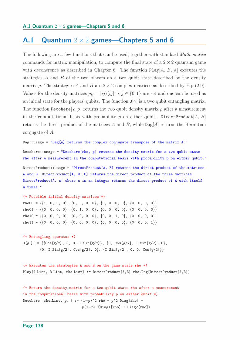
A.1 Quantum 2 × 2 games—Chapters 5 and 6
A.1 Quantum 2 × 2 games—Chapters 5 and 6
The following are a few functions that can be used, together with standard Mathematica
commands for matrix manipulation, to compute the final state of a 2 × 2 quantum game
with decoherence as described in Chapter 6. The function Play[A, B, ρ ] executes the
strategies A and B of the two players on a two qubit state described by the density
matrix ρ. The strategies A and B are 2 × 2 complex matrices as described by Eq. (2.9).
Values for the density matrices ρij = |ij〉〈ij|, i, j ∈ 0, 1 are set and one can be used as
an initial state for the players’ qubits. The function J[γ] is a two qubit entangling matrix.
The function Decohere[ ρ, p ] returns the two qubit density matrix ρ after a measurement
in the computational basis with probability p on either qubit. DirectProduct[A, B]
returns the direct product of the matrices A and B, while Dag[A] returns the Hermitian
conjugate of A.
Dag::usage = "Dag[A] returns the complex conjugate transpose of the matrix A."
Decohere::usage = "Decohere[rho, p] returns the density matrix for a two qubit state
rho after a measurement in the computational basis with probability p on either qubit."
DirectProduct::usage = "DirectProduct[A, B] returns the direct product of the matrices
A and B. DirectProduct[A, B, C] returns the direct product of the three matrices.
DirectProduct[A, n] where n is an integer returns the direct product of A with itself
n times."
(* Possible initial density matrices *)
rho00 = 1, 0, 0, 0, 0, 0, 0, 0, 0, 0, 0, 0, 0, 0, 0, 0rho01 = 0, 0, 0, 0, 0, 1, 0, 0, 0, 0, 0, 0, 0, 0, 0, 0rho10 = 0, 0, 0, 0, 0, 0, 0, 0, 0, 0, 1, 0, 0, 0, 0, 0rho11 = 0, 0, 0, 0, 0, 0, 0, 0, 0, 0, 0, 0, 0, 0, 0, 1
(* Entangling operator *)
J[g ] := Cos[g/2], 0, 0, I Sin[g/2], 0, Cos[g/2], I Sin[g/2], 0,0, I Sin[g/2], Cos[g/2], 0, I Sin[g/2], 0, 0, Cos[g/2]
(* Executes the strategies A and B on the game state rho *)
Play[A List, B List, rho List] := DirectProduct[A,B].rho.Dag[DirectProduct[A,B]]
(* Return the density matrix for a two qubit state rho after a measurement
in the computational basis with probability p on either qubit *)
Decohere[ rho List, p ] := (1−p)^2 rho + p^2 Diag[rho] +
p(1−p) (Diag1[rho] + Diag2[rho])
Page 138

Appendix A Software routines
(* Various functions of a square (density) matrix A *)
Diag[ A ] := Table[ If[ i == j, A[[i,j]], 0 ], i, Length[A], j, Length[A] ]
Diag1[ A ] := Table[ If[ Floor[(i+1)/2] == Floor[(j+1)/2], A[[i,j]], 0 ],
i, Length[A], j, Length[A] ]
Diag2[ A ] := Table[ If[ (i == j)||(Abs[i−j] == 2), A[[i,j]], 0 ],
i, Length[A], j, Length[A] ]
Dag[ A ] := Transpose[ A /. I −> ZZ /. −I −> I, ZZ −> −I ]
(* Rules for the direct product *)
DirectProduct[ A List ] := A
DirectProduct[ A List, 1 ] := A
DirectProduct[ A List, n Integer ] :=
Module[
AA = A ,Do[ AA = DirectProduct[AA, A], i,2,n ];
AA
]
DirectProduct[ A List, B List ] :=
Module[
M,
nr=Length[A], nc=Length[ A[[1]] ],
mr=Length[B], mc=Length[ B[[1]] ] ,Do[
M[ (i−1)mr+k, (j−1)mc+l ] = A[[i,j]] B[[k,l]],
l,mc, k,mr, j,nc, i,nr];
Array[ M, nr mr, nc mc ]
]
DirectProduct[ A List, B List, CC List ] := DirectProduct[ DirectProduct[A,B], CC ]
A.2 Classical Parrondo’s games—Chapter 7
A.2.1 Capital-dependent game—Section 7.2.1
This package is used to generate the expected return versus time for a mixture of game
A and the capital-dependent game B. A one-dimensional array is required to hold the
probability of having capitals from −n to n, where n is the maximum number of games
to be played. This is set up by the Start[n] command for an initial capital of 0. The
command Results[c, p, . . . , n] generates a list of the expected payoffs for n steps of the
Page 139
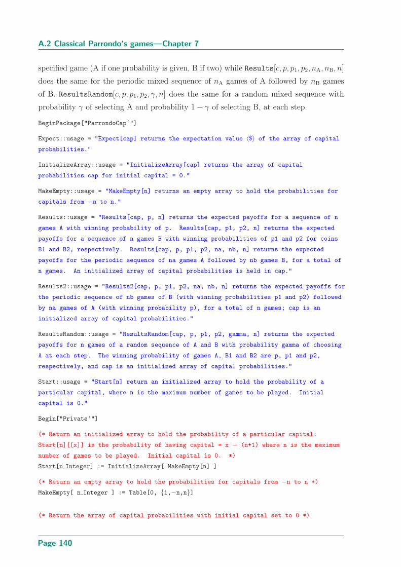
A.2 Classical Parrondo’s games—Chapter 7
specified game (A if one probability is given, B if two) while Results[c, p, p1, p2, nA, nB, n]
does the same for the periodic mixed sequence of nA games of A followed by nB games
of B. ResultsRandom[c, p, p1, p2, γ, n] does the same for a random mixed sequence with
probability γ of selecting A and probability 1 − γ of selecting B, at each step.
BeginPackage["ParrondoCap‘"]
Expect::usage = "Expect[cap] returns the expectation value 〈$〉 of the array of capital
probabilities."
InitializeArray::usage = "InitializeArray[cap] returns the array of capital
probabilities cap for initial capital = 0."
MakeEmpty::usage = "MakeEmpty[n] returns an empty array to hold the probabilities for
capitals from −n to n."
Results::usage = "Results[cap, p, n] returns the expected payoffs for a sequence of n
games A with winning probability of p. Results[cap, p1, p2, n] returns the expected
payoffs for a sequence of n games B with winning probabilities of p1 and p2 for coins
B1 and B2, respectively. Results[cap, p, p1, p2, na, nb, n] returns the expected
payoffs for the periodic sequence of na games A followed by nb games B, for a total of
n games. An initialized array of capital probabilities is held in cap."
Results2::usage = "Results2[cap, p, p1, p2, na, nb, n] returns the expected payoffs for
the periodic sequence of nb games of B (with winning probabilities p1 and p2) followed
by na games of A (with winning probability p), for a total of n games; cap is an
initialized array of capital probabilities."
ResultsRandom::usage = "ResultsRandom[cap, p, p1, p2, gamma, n] returns the expected
payoffs for n games of a random sequence of A and B with probability gamma of choosing
A at each step. The winning probability of games A, B1 and B2 are p, p1 and p2,
respectively, and cap is an initialized array of capital probabilities."
Start::usage = "Start[n] return an initialized array to hold the probability of a
particular capital, where n is the maximum number of games to be played. Initial
capital is 0."
Begin["Private‘"]
(* Return an initialized array to hold the probability of a particular capital:
Start[n][[x]] is the probability of having capital = x − (n+1) where n is the maximum
number of games to be played. Initial capital is 0. *)
Start[n Integer] := InitializeArray[ MakeEmpty[n] ]
(* Return an empty array to hold the probabilities for capitals from −n to n *)
MakeEmpty[ n Integer ] := Table[0, i,−n,n]
(* Return the array of capital probabilities with initial capital set to 0 *)
Page 140

Appendix A Software routines
InitializeArray[ cap List ] :=
Module[
nc = cap ,nc[[ (Length[nc] + 1)/2 ]] = 1;
nc
]
(* Return the array of capital probabilities with initial capital set to -1,0,+1
each with probability 1/3 *)
InitializeArray2[ cap List ] :=
Module[
nc = cap, n = (Length[nc]−1)/2 ,nc[[n]] = 1/3;
nc[[n+1]] = 1/3;
nc[[n+2]] = 1/3;
nc
]
(* Return a list of expected payoffs for n steps of game A *)
Results[ cap List, p , n Integer ] := Results[cap, p, p, n]
(* Return a list of expected payoffs for n steps of game B *)
Results[ cap List, p1 , p2 , n Integer ] :=
Module[
results = Table[0, i,n], nc = cap ,Do[ nc = NextStep[ nc, p1, p2];
results[[i]] = Expect[nc],
i,n];
results
]
(* Return a list of expected payoffs for n steps of a periodic sequence
of na games of A followed by nb games of B for a total of n games *)
Results[ cap List, p , p1 , p2 , na Integer, nb Integer, n Integer ] :=
Module[
results = Table[0, i,n],nseries = Floor[n/(na+nb)],
nc=cap ,Do[
Do[ nc = NextStep[nc, p, p];
results[[i+j]] = Expect[nc],
Page 141

A.2 Classical Parrondo’s games—Chapter 7
j,na];
Do[ nc = NextStep[nc, p1, p2];
results[[i+na+k]] = Expect[nc],
k,nb],
i, 0, (nseries−1)(na+nb), (na+nb)];
results
]
(* Return a list of expected payoffs for n steps of a periodic sequence
of nb games of B followed by na games of A for a total of n games *)
Results2[ cap List, p , p1 , p2 , na Integer, nb Integer, n Integer ] :=
Module[
results = Table[0, i,n],nseries = Floor[n/(na+nb)],
nc=cap ,Do[
Do[ nc = NextStep[nc, p1, p2];
results[[i+j]] = Expect[nc],
j,nb];
Do[ nc = NextStep[nc, p, p];
results[[i+nb+k]] = Expect[nc],
k,na],
i, 0, (nseries−1)(na+nb), (na+nb)];
results
]
(* Return a list of expected payoffs for n steps of a random mixed sequence
of games A and B, with a probability gamma of selecting A at each step *)
ResultsRandom[ cap , p , p1 , p2 , gamma , n Integer ] :=
Module[
results = Table[0, i,n], nc = cap ,Do[ nc = gamma * NextStep[nc, p] + (1−gamma) * NextStep[nc, p1, p2];
results[[i]] = Expect[nc],
i,n];
results
]
Page 142
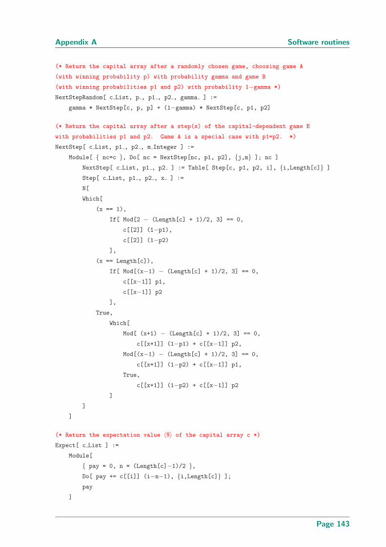
Appendix A Software routines
(* Return the capital array after a randomly chosen game, choosing game A
(with winning probability p) with probability gamma and game B
(with winning probabilities p1 and p2) with probability 1−gamma *)
NextStepRandom[ c List, p , p1 , p2 , gamma ] :=
gamma * NextStep[c, p, p] + (1−gamma) * NextStep[c, p1, p2]
(* Return the capital array after a step(s) of the capital-dependent game B
with probabilities p1 and p2. Game A is a special case with p1=p2. *)
NextStep[ c List, p1 , p2 , m Integer ] :=
Module[ nc=c , Do[ nc = NextStep[nc, p1, p2], j,m ]; nc ]
NextStep[ c List, p1 , p2 ] := Table[ Step[c, p1, p2, i], i,Length[c] ]
Step[ c List, p1 , p2 , x ] :=
N[
Which[
(x == 1),
If[ Mod[2 − (Length[c] + 1)/2, 3] == 0,
c[[2]] (1−p1),c[[2]] (1−p2)
],
(x == Length[c]),
If[ Mod[(x−1) − (Length[c] + 1)/2, 3] == 0,
c[[x−1]] p1,
c[[x−1]] p2
],
True,
Which[
Mod[ (x+1) − (Length[c] + 1)/2, 3] == 0,
c[[x+1]] (1−p1) + c[[x−1]] p2,
Mod[(x−1) − (Length[c] + 1)/2, 3] == 0,
c[[x+1]] (1−p2) + c[[x−1]] p1,
True,
c[[x+1]] (1−p2) + c[[x−1]] p2
]
]
]
(* Return the expectation value 〈$〉 of the capital array c *)
Expect[ c List ] :=
Module[
pay = 0, n = (Length[c]−1)/2 ,Do[ pay += c[[i]] (i−n−1), i,Length[c] ];
pay
]
Page 143

A.2 Classical Parrondo’s games—Chapter 7
End[]
EndPackage[]
A.2.2 History-dependent game—Section 7.2.2
This package is used to generate the expected return versus time for a mixture of game A
and the history-dependent game B, or for a mixture of two history-dependent games (see
Sec. 7.2.2). The commands are very similar to the capital-dependent game except with the
addition of extra probabilities in game B. The command Results can be used as before to
return a list of expected payoffs for game A, B or a mixture. By specifying two sets of prob-
abilities for the history-dependent game, Results[c, p1, p2, p3, p4, p′1, p
′2, p
′3, p
′4, nB, nB′ , n]
returns a list of the expected payoffs for n steps of the periodic sequence of nB games of
B followed nB′ games of B′. Similarly, by specifying two sets of history-dependent proba-
bilities in ResultsRandom a random mixture of the two history-dependent games can be
considered.
BeginPackage["ParrondoHist‘"]
Expect::usage = "Expect[cap] returns the expectation value 〈$〉 of the array of capital
probabilities."
InitializeArray::usage = "InitializeArray[cap] returns the array of capital
probabilities cap for initial capital = 0."
MakeEmpty::usage = "MakeEmpty[n] returns an empty array to hold the probabilities for
capitals from -n to n."
Results::usage = "Results[cap, p, n] returns the expected payoffs for a sequence of
game A with winning probability p. Results[cap, p1, p2, p3, p4, n] returns the
expected payoffs for a sequence of game B with winning probabilities p1, p2, p3 and p4,
for coins B1, B2, B3 and B4, respectively. Results[cap, p, p1, p2, p3 p4, na, nb, n]
returns the expected payoffs for the periodic sequence of na games of A followed by nb
games of B. Results[cap, q1, q2, q3, q4, p1, p2, p3, p4, n1, n2, n] returns the
expected payoffs for a periodic sequence of n1 games of B with winning probabilities q1,
q2, q3 and q4, followed by n2 game of B with winning probabilities p1, p2, p3 and p4.
The total number of games is n and cap is an initialized array of capital
probabilities."
Results2::usage = "Results2[cap, p, p1, p2, p3, p4, na, nb, n] returns the expected
payoffs for the periodic sequence of nb games of B (with winning probabilities p1, p2,
p3 and p4) followed by na games of A (with winning probability p). The total number of
games is n and cap is an initialized array of capital probabilities."
Page 144

Appendix A Software routines
ResultsRandom::usage = "ResultsRandom[cap, p, p1, p2, p3, p4, gamma, n] returns the
expected payoffs for n games of a random sequence of A and B with probability gamma of
choosing A at each step. The winning probabilities are p for game A, and for p1, p2,
p3 and p4 for game B; cap is an initialized array of capital probabilities.
ResultsRandom[cap, q1, q2, q3, q4, p1, p2, p3, p4, gamma, n] returns the expected
payoffs for a random mixed sequence of two games B (with probabilities q1, q2, q3, and
q4, or p1, p2, p3, and p4), selecting the first game with probability gamma at each
step."
Start::usage = "Start[n] returns an initialized array to hold the probability of a
particular capital, where n is the maximum number of games to be played. Initial
capital is 0."
Begin["Private‘"]
(* Return an initialized array to hold the probability of a particular capital:
Start[n][[x]] is the probability of having capital = x − (n+1) where n is the
maximum number of games to be played. Initial capital is 0 *)
Start[ n Integer ] := Table[ If[ i == n+1, 1, 0 ], i,2n+1 ]
(* Set up a history vector holding the results of the last two games: preferred
starting point is to take an equal mixture of the four possible histories *)
inithist = 1/4,1/4,1/4,1/4
(* History-dependent game B with winning probabilities p1 after (loss, loss),
p2 after (loss, win), p3 after (win, loss), p4 after (win, win) *)
B[ p1 , p2 , p3 , p4 ] :=
1−p1, 0, 1−p3, 0, p1, 0, p3, 0, 0, 1−p2, 0, 1−p4, 0, p2, 0, p4
(* Game A is a special case of game B with all the probabilities the same *)
A[ p ] := B[p, p, p, p]
(* Return a list of expected payoff versus t for a sequence of n games A *)
Results[ cap List, hist List, p , n Integer ] := Results[cap, hist, p, p, p, p, n]
(* Return a list of expected payoff versus t for a sequence of n games B *)
Results[ cap List, hist List, p1 , p2 , p3 , p4 , n Integer ] :=
Module[ results = Table[0,i,n], nc = cap, h = hist ,Do[ h = B[p1, p2, p3, p4].h;
nc = NextStep[nc, Win[h]];
results[[i]] = Expect[nc],
i,n];
results
]
Page 145
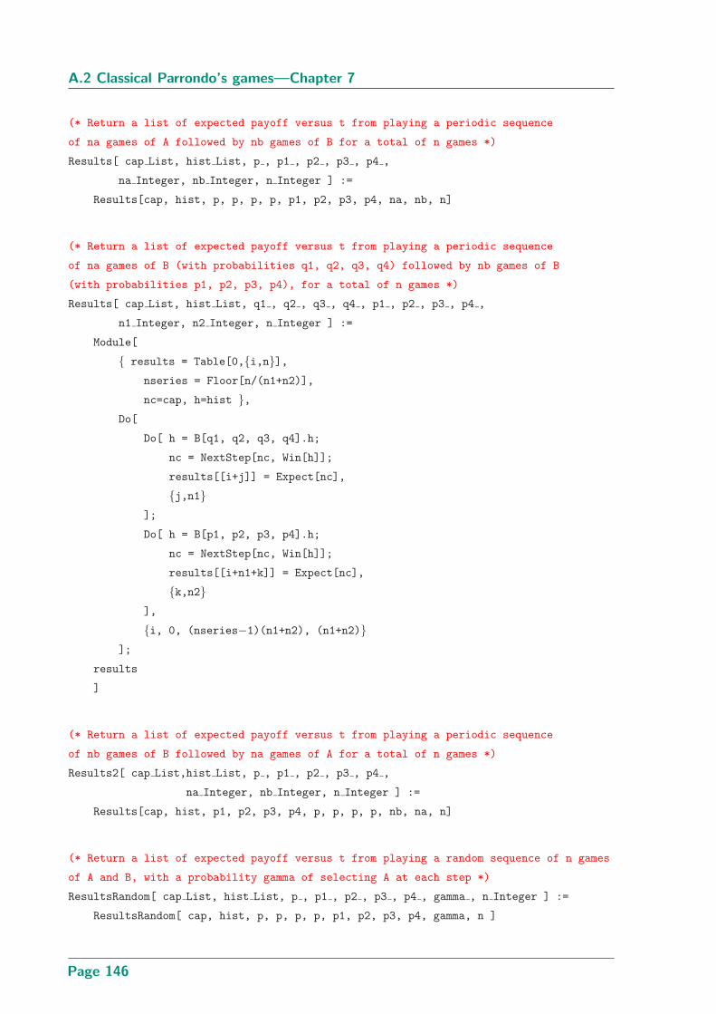
A.2 Classical Parrondo’s games—Chapter 7
(* Return a list of expected payoff versus t from playing a periodic sequence
of na games of A followed by nb games of B for a total of n games *)
Results[ cap List, hist List, p , p1 , p2 , p3 , p4 ,
na Integer, nb Integer, n Integer ] :=
Results[cap, hist, p, p, p, p, p1, p2, p3, p4, na, nb, n]
(* Return a list of expected payoff versus t from playing a periodic sequence
of na games of B (with probabilities q1, q2, q3, q4) followed by nb games of B
(with probabilities p1, p2, p3, p4), for a total of n games *)
Results[ cap List, hist List, q1 , q2 , q3 , q4 , p1 , p2 , p3 , p4 ,
n1 Integer, n2 Integer, n Integer ] :=
Module[
results = Table[0,i,n],nseries = Floor[n/(n1+n2)],
nc=cap, h=hist ,Do[
Do[ h = B[q1, q2, q3, q4].h;
nc = NextStep[nc, Win[h]];
results[[i+j]] = Expect[nc],
j,n1];
Do[ h = B[p1, p2, p3, p4].h;
nc = NextStep[nc, Win[h]];
results[[i+n1+k]] = Expect[nc],
k,n2],
i, 0, (nseries−1)(n1+n2), (n1+n2)];
results
]
(* Return a list of expected payoff versus t from playing a periodic sequence
of nb games of B followed by na games of A for a total of n games *)
Results2[ cap List,hist List, p , p1 , p2 , p3 , p4 ,
na Integer, nb Integer, n Integer ] :=
Results[cap, hist, p1, p2, p3, p4, p, p, p, p, nb, na, n]
(* Return a list of expected payoff versus t from playing a random sequence of n games
of A and B, with a probability gamma of selecting A at each step *)
ResultsRandom[ cap List, hist List, p , p1 , p2 , p3 , p4 , gamma , n Integer ] :=
ResultsRandom[ cap, hist, p, p, p, p, p1, p2, p3, p4, gamma, n ]
Page 146
Appendix A Software routines
(* Return a list of expected payoff versus t from playing a random mixed sequence of
two different games B (with probs q1, q2, q3, q4 chosen with frequency gamma, or with
probs p1, p2, p3, p4 chosen with frequency 1−gamma) for a total of n games *)
ResultsRandom[ cap List, hist List, q1 , q2 , q3 , q4 , p1 , p2 , p3 , p4 ,
gamma , n Integer ] :=
Module[
results = Table[0,i,n],qp1 = gamma q1 + (1−gamma) p1,
qp2 = gamma q2 + (1−gamma) p2,
qp3 = gamma q3 + (1−gamma) p3,
qp4 = gamma q4 + (1−gamma) p4,
nc=cap, h=hist ,Do[ h = B[qp1, qp2, qp3, qp4].h;
nc = NextStep[nc, Win[h]];
results[[i]] = Expect[nc],
i,n];
results
]
(* Update the array of capital probabilities c according to the winning probs w *)
NextStep[ c List, w , m Integer ] :=
Module[ nc=c, Do[ nc = NextStep[nc, w], j,m ]; nc ]
NextStep[ c List, w ] := Table[ Step[c, w, i], i,Length[c] ]
Step[ c List, w , x ] :=
N[
Which[
(x == 1),
c[[x+1]] (1-w),
(x == Length[c]),
c[[x−1]] w,
True,
c[[x+1]] (1-w) + c[[x−1]] w
]
]
(* Return the probability of a win based on the history vector h *)
Win[ h List ] := h[[2,1]] + h[[4,1]]
(* Return the expectation value 〈$〉 of the capital array c *)
Expect[ c List ] :=
Module[
Page 147

A.3 Quantum walks—Section 7.3.1 and Chapter 8
pay = 0, n = (Length[c]−1)/2 ,Do[ pay += c[[i]] (i−n−1), i,Length[c] ];
pay
]
End[]
EndPackage[]
A.3 Quantum walks—Section 7.3.1 and Chapter 8
The package below contains functions that execute the history-dependent quantum walk
or the quantum walk with a position-dependent potential. A combination of two walks
to create a quantum Parrondo’s game can also be executed. An array to contain the x
amplitudes is created by the functions SymStart[n] or AntStart[n], for a starting start
that is, respectively, symmetric or antisymmetric under the interchange of L ↔ R. The
function Results[c, ρ, n] returns a list of expectation values of x for n steps of the quantum
walk starting with the state c and governed by the list of probabilities ρ (e.g., for M = 3, ρ
is a list of the four probabilities ρLL, ρLR, ρRL, ρRR). The position-dependent potentials
of Eq. (7.4) with parameters α and β can be applied by Results[c, ρ, α, β, n]. A periodic
mixture of two different walks is carried out by Results[c, ρ1, ρ2, n1, n2, n]. The package
includes several plotting functions to display various features of the quantum walks, of
which the most useful is PlotProbs[c] that plots the probability density distribution for
the state c.
BeginPackage["QuantumWalk‘"]
AntStart::usage = "AntStart[n, m] returns an initialized array (with starting state
anti-symmetric) to hold the amplitudes for positions from −n to n for m coins."
SymStart::usage = "SymStart[n, m] returns an initialized array (with symmetric starting
state) to hold the amplitudes for positions from −n to n for m coins."
MakeEmpty::usage = "MakeEmpty[n, m] returns an empy array to hold the amplitudes for
positions from −n to n for m coins."
ExtendArray::usage = "ExtendArray[cap, n] extends the array of amplitudes cap by an
additional n positions (+ and −)."
Start::usage = "Start[n, st] returns an initialized array for m=Log[2, Length[st]]
coins for positions from −n to n with a normalized starting state at x=0 whose
relative amplitudes and phases are specified by the list st."
Page 148
Appendix A Software routines
Results::usage = "Results[cap, p, n] returns a list of 〈x〉 for a sequence of n steps
with probabilities specified by the list p. Results[cap, p, a, b, n] is the same but
with a biased sawtooth potential depending on a and b, as per Meyer’s scheme.
Results[cap, q, p, na, nb, n] does na steps
with probabilities q, followed by nb steps with probabilities p, repeating the sequence
n times. The p an q are lists of history-dependent probabilities; cap is a an
initialized array of x amplitudes."
ResultsRandom::usage = "ResultsRandom[cap, gamma, q, p, n] returns a list of 〈x〉 for a
random mixture of steps with probabilities specified by the lists q or p, the first
being chosen with probability gamma and the second with probability 1−gamma. The total
number of steps in n and cap is an initialized array of x amplitudes."
NextStep::usage = "NextStep[cap, p] returns the position array cap after one step with
probabilities specified by the list p. NextStep[cap, p, n] returns the array after
n steps. NextStep[cap, p, a, b, n] returns the array after n steps with the addition
of a biased sawtooth potential specified by a and b."
Expect::usage = "Expect[cap] returns 〈x〉 for the array of position amplitudes cap."
PlotSmooth::usage = "PlotSmooth[cap, range, color] plots the distribution of position
probabilities for the array cap, smoothing by (p(x−1) + 2 p(x) + p(x+1))/4.
Specifying a range ymin,ymax or color
(e.g., Red, RGBColor[0,0,1]) is optional."
PlotProb::usage = "PlotProb[cap, range, color] plots the distribution of probabilities
for the array of position amplitudes cap. Specifying a range ymin,ymax or color (e.g.
Red, RGBColor[0,0,1] etc.) is optional."
ProbDist::usage = "ProbDist[cap, p, n, int] plots the distribution of position
probabilities after every int moves for a starting array cap and probabilities
specified by the list p for a total of n moves. ProbDist[cap, p, a, n, int] adds a
biasing potential V(x) = a x."
ProbRange::usage = "ProbRange[cap, x, y] returns the probability that the particle is
located between x and y."
Begin["Private‘"]
(* Create an empy array to hold amplitudes for positions from −n to +n *)
MakeEmpty[ n Integer, m Integer ] := Table[0, i,−n,n, j, 2^m]
(* Return a starting array symmetric in past histories *)
SymStart[ n Integer, m Integer ]:=
Table[ If[ i == 0, (1/Sqrt[2])^m, 0 ], i,−n,n,j, 2^m ]
(* Return a starting array anti-symmetric in the momentum direction for each
Page 149

A.3 Quantum walks—Section 7.3.1 and Chapter 8
momentum in the history *)
AntStart[ n Integer, m Integer ] :=
Table[
If[ i == 0,
Antisym[m]/Sqrt[2]^m,
Table[0, i, 2^m]],
i,−n,n]
Antisym[ m Integer ] := Table[ (−1)^Parit[i−1], i, 2^m ]
Parit[ m Integer ] := Sum[ IntegerDigits[m, 2][[j]], j, Length[IntegerDigits[m,2]] ]
(* Return an initialized starting array for capitals from −n to n with an arbitrary
starting combination at x=0 specified by the list st of 2^m elements *)
Start[ n Integer, st List ] :=
Table[
If[ i == 0,
st/Sqrt[ Sum[ Abs[st[[i]]]^2, i,Length[st] ] ],
Table[ 0, i,Length[st] ]
],
i,−n,n]
(* Extend an existing array of capitals *)
ExtendArray[ cap List, n Integer ] :=
Table[
If[ (j <= n) || (j > n + Length[cap]),
Table[ 0, i,Length[cap[[1]]] ],
cap[[j − n]]
],
j, Length[cap] + 2 n]
(* Return the expectation values of x for a sequence of n steps *)
Results[ cap List, p List, n Integer ] :=
Module[ results = Table[0,i,n], nc=cap, j ,Do[ nc = NextStep[nc, p];
results[[j]] = Expect[nc],
j,n];
results
]
Page 150

Appendix A Software routines
(* Add a potential specified by a and b *)
Results[ cap List, p List, a , b , n Integer ] :=
Module[ results = Table[0,i,n], nc=cap, j ,Do[ nc = NextStep[nc, p, a, b];
results[[j]] = Expect[nc],
j,n];
results
]
(* Return <x> for a periodic mixed sequence of two walks, with na steps with
probabilities q followed by nb steps with probabilities p, for a total of n steps *)
Results[ cap List, q List, p List,
na Integer, nb Integer, n Integer ] :=
Module[
results = Table[0,i,n],nseries = Floor[n/(na+nb)],
nc=cap ,Do[
Do[
nc = NextStep[nc, q];
results[[(i−1)(na+nb)+j]] = Expect[nc],
j,na];
Do[
nc = NextStep[nc, p];
results[[(i−1)(na+nb)+na+k]] = Expect[nc],
k,nb],
i,nseries];
results
]
(* Add potentials specified by a1, b1 and a2, b2 *)
Results[ cap List, q List, a1 , b1 , p List, a2 , b2 ,
na Integer, nb Integer, n Integer ] :=
Module[
results = Table[0,i,n],nseries = Floor[n/(na+nb)],
nc=cap ,Do[
Page 151
A.3 Quantum walks—Section 7.3.1 and Chapter 8
Do[
nc = NextStep[nc, q, a1, b1];
results[[(i−1)(na+nb)+j]] = Expect[nc],
j,na];
Do[ nc = NextStep[nc, p, a2, b2];
results[[(i−1)(na+nb)+na+k]] = Expect[nc],
k,nb],
i,nseries];
results
]
(* Return <x> for a random mixed sequence of walks with probabilities q or p,
selecting the 1st with probability gamma and the 2nd with probability 1−gamma) *)
ResultsRandom[ cap , q List, p List, gamma n Integer ] :=
Module[
results = Table[0, i,n],nc=cap ,
Do[
If[
Random[] < gamma,
nc = NextStep[nc, q],
nc = NextStep[nc, p]
];
results[[j]] = Expect[nc],
j,n];
results
]
(* Add potentials specified by a1, b1 and a2, b2 *)
ResultsRandom[ cap , q List, a1 , b1 , p List, a2 , b2 , gamma , n Integer ] :=
Module[
results = Table[0, i,n], nc=cap ,Do[
If[
Random[] < gamma,
nc = NextStep[nc, q, a1, b1],
nc = NextStep[nc, p, a2, b2]
Page 152
Appendix A Software routines
];
results[[j]] = Expect[nc],
j,n];
results
]
(* Take a step(s) in array c with probability list p and (optional) potential
specified by a and b *)
NextStep[ c List, p List, m Integer ] :=
Module[ nc=c, Do[ nc = NextStep[nc, p, 0, 0], k,m ]; nc ]
NextStep[ c List, p List, a , b , m Integer ] :=
Module[ nc=c, Do[ nc = NextStep[nc, p, a, b], k,m ]; nc ]
NextStep[ c List, p List] := Table[ Step[c, p, 0, 0, i], i,Length[c] ]
NextStep[ c List, p List, a , b ] := Table[ Step[c, p, a, b, i], i,Length[c] ]
Step[ c , p , x ] :=
Module[
m = Length[c[[x]]] ,N[
Table[
If[ j <= m/2,
If[ x == Length[c],
0,
Sqrt[p[[j]]] c[[x+1, 2j−1]] +
I Sqrt[1−p[[j]]] c[[x+1, 2j]]
],
If[ x == 1,
0,
I Sqrt[1−p[[j−m/2]]] c[[x−1, 2j−m−1]] +
Sqrt[p[[j−m/2]]] c[[x−1, 2j−m]]]
],
j,m]
]
]
Step[ c , p , a , b , x ] :=
Module[
m = Length[c[[x]]],
v1 = Exp[−I V[c, x+1, a, b] ],
v2 = Exp[−I V[c, x−1, a, b] ] ,N[
Page 153

A.3 Quantum walks—Section 7.3.1 and Chapter 8
Table[
If[ j <= m/2,
If[ x == Length[c],
0,
v1 (Sqrt[p[[j]]] c[[x+1, 2j−1]] +
I Sqrt[1−p[[j]]] c[[x+1, 2j]])
],
If[ x == 1,
0,
v2 (I Sqrt[1−p[[j−m/2]]] c[[x−1, 2j−m−1]] +
Sqrt[p[[j−m/2]]] c[[x−1, 2j−m]])]
],
j,m]
]
]
(* Return the value of the potential specified by a and b, at a position z:
b=0 gives VA (linear x-dependent potential), b>0 gives VB (sawtooth potential),
b<0 gives V(x) = a P(x) *)
V[ c , z , a , b ] :=
If[ b == −1,If[ (z > 0)&&(z <= Length[c]),
a Sum[ Abs[c[[z,k]]^2], k,Length[c[[1]]] ],
0
],
a (z−(Length[c]+1)/2) + b (1−Mod[z−(Length[c]+1)/2, 3]/2)
]
(* Additional potentials *)
(* Step function at x=a of height b (Pi/2 is infinite?) *)
V1[ c , z , a , b ] := If[ z >= (Length[c]+1)/2 + a, b, 0 ]
(* Barrier of width 10 at x=a of height b *)
V2[ c , z , a , b ] :=
If[ (z >= (Length[c]+1)/2 + a) && (z <= (Length[c]+1)/2 + a + 10), b, 0 ]
(* Return <x> for array c, assumed to be numerical *)
Expect[ c List ] :=
Sum[
Abs[ c[[i,j]]^2 ] (i−(Length[c]+1)/2),
Page 154
Appendix A Software routines
j,Length[c[[1]]], i,Length[c]]
(* Return the variance for array c, assumed numerical *)
Variance[c List] := Expect[c,2] − Expect[c]^2
(* Return the k-th moment of c *)
Expect[ c List, k Integer ] :=
Sum[
Abs[ c[[i,j]]^2 ] (i−(Length[c]+1)/2)^k,j,Length[c[[1]]], i,Length[c]
]
Moment[ p List, k Integer ] :=
Sum[ p[[i,2]] p[[i,1]]^k, i,Length[p] ]/Length[p]
(* Return the probability that the particle is located between x and y *)
ProbRange[ c , x , y ] :=
Sum[ Abs[ c[[j,k]]^2 ], k,Length[c[[1]]],j, (Length[c]+1)/2 + x, (Length[c]+1)/2 + y ]
(* Plot the probability densities for the range of x-values smoothing by a weighted
average; can also plot two distributions on the same graph in different colors *)
<<Graphics‘MultipleListPlot‘
PlotSmooth[ c ] := PlotSmooth[ c, All, Black ]
PlotSmooth[ c , range List ] := PlotSmooth[ c, range, Black ]
PlotSmooth[ c , color ] := PlotSmooth[ c, All, color ]
PlotSmooth[ c , range , color ] :=
ListPlot[
Smooth[ Probs[c] ],
PlotJoined −> True,
AxesLabel −> "x", "P",PlotRange −> range,
PlotStyle −> color
]
PlotSmooth[ c1 , c2 , range , color1 , color2 ] :=
MultipleListPlot[
Smooth[ Probs[c1] ], Smooth[ Probs[c2] ],
PlotJoined −> True,
AxesLabel −> "x", "P",SymbolShape −> None,
PlotRange −> range,
PlotStyle −> color1, color2]
Page 155
A.3 Quantum walks—Section 7.3.1 and Chapter 8
(* Plot the probability densities for the range of x values,
plotting odd or even points depending on which are non-zero *)
PlotProb[ c List ] := PlotProb[ c, All, Black ]
PlotProb[ c List, range List ] := PlotProb[ c, range, Black ]
PlotProb[ c List, color ] := PlotProb[ c, All, color ]
PlotProb[ c List, range , color ] :=
ListPlot[
If[ ProbRange[c,0,0] == 0, EvenList[Probs[c]], OddList[Probs[c]] ],
PlotJoined −> True,
AxesLabel −> "x", "P",PlotRange −> range,
PlotStyle −> color
]
PlotProb[ c1 List, c2 List, range , color1 , color2 ] :=
MultipleListPlot[
If[ ProbRange[c1,0,0] == 0,
EvenList[Probs[c1]],
OddList[Probs[c1]]
],
If[ ProbRange[c2,0,0] == 0,
EvenList[Probs[c2]],
OddList[Probs[c2]]
],
PlotJoined −> True,
AxesLabel −> "x", "P",SymbolShape −> None,
PlotRange −> range,
PlotStyle −> color1, color2]
(* Show successive probability distributions as they evolve, plotting in colors
successively changing from red to blue *)
ProbDist[ c List, p List, n , int ] := ProbDist[ c, p, 0, 0, n, int, 0.3 ]
ProbDist[ c List, p List, n , int , maxy ] := ProbDist[ c, p, 0, 0, n, int, maxy ]
ProbDist[ c List, p List, a , b , n , int ] := ProbDist[ c, p, a, b, n, int, 0.3 ]
ProbDist[ c List, p List, a , b , n , int , maxy ] :=
Module[ nc=c ,Do[
nc = NextStep[nc, p, a, b, int];
PlotProb[ nc, −(Length[nc]−1)/2, (Length[nc]−1)/2,0,maxy, Red ];
Print["t = ", j*int],
Page 156

Appendix A Software routines
j,Floor[n/int]];
nc
]
(* Return a list of probabilities *)
Probs[ c ] := Table[ j−(Length[c]+1)/2, Sum[ Abs[c[[j,k]]^2], k,Length[c[[1]]] ],j,Length[c] ]
(* Return the odd or even points in a list---i.e. the non−zero points *)
OddList[ l ] := Table[ l[[i]], i,1,Length[l],2 ]
EvenList[ l ] := Table[ l[[i]], i,2,Length[l],2 ]
(* Return a list of smoothed probabilities *)
Smooth[ c ] := Table[ (c[[j−1]] + 2 c[[j]] + c[[j+1]])/4, j,2,Length[c]−1 ]
(* Return the position of a peak between x=n1 and x=n2 in the prob distribution p *)
PeakPosn[ p List, n1 , n2 ] :=
p[[ Ordering[ Table[ p[[j, 2]], j, n1 + (Length[p] + 1)/2,
n2 + (Length[p] + 1)/2], −1] + n1 + (Length[p] − 1)/2 , 1]]
(* Plot the position of a peak between n1*t/10 and n2*t/10 as a function of t *)
PlotPeakPosn[ c List, n1 , n2 , color ] :=
ListPlot[
Flatten[ Table[ PeakPosn[Probs[c[[i]]], i*n1, i*n2], i, Length[c] ] ],
PlotJoined −> True, AxesLabel −> "t", "x", PlotStyle −> color,
Ticks −> 1, "", 2, "", 3, "", 4, "", 5, "50",6, "", 7, "", 8, "", 9, "", 10, "100", 11, "",12, "", 13, "", 14, "", 15, "150", 16, "", 17, "",18, "", 19, "", 20, "200", Automatic
]
(* Return x position of the peak and summed probability under the peak *)
GetPeak[ xp List, n1 Integer, n2 Integer, cut ] :=
Module[
m1 = n1 + (Length[xp]+1)/2,
m2 = n2 + (Length[xp]+1)/2,
posnmax = Ordering[ Table[ xp[[j,2]], j,m1,m2 ], −1 ][[1]] + m1 , posnmax−(Length[xp]−1)/2,
Sum[ xp[[j, 2]], j, posnmax + GetCutOff[xp, posnmax, cut, −2],posnmax + GetCutOff[xp, posnmax, cut, +2] ]
]
Page 157

A.4 Quantum cellular automata—Chapter 9
(* Return the cutoff for the peak in the direction specified by step with a cutoff
ratio of c *)
GetCutOff[ p List, pmax , c , step ] :=
Module[
width, m ,For[
width=0; m=(Length[p]+1)/2,
p[[pmax−width,2]]/p[[pmax,2]] > c,
width += step
];
width
]
(* Quantify the difference between two probability distributions ---
the second function is chi squared between the two curves *)
ProbDiff[ p1 List, p2 List ] :=
Sum[ Abs[p1[[i,2]]−p2[[i,2]]], i, Min[Length[p1], Length[p2]] ]
ChiSq[ p1 List, p2 List ] :=
Sum[ (p1[[i,2]]−p2[[i,2]])^2, i, Min[Length[p1], Length[p2]] ]
End[]
EndPackage[]
A.4 Quantum cellular automata—Chapter 9
A.4.1 One-dimensional QCA—Section 9.1.3
This package implements the one-dimensional quantum cellular automata described in
Schumacher and Werner (2004) and shown schematically in Figure 9.5. The function
MakeEmpty[n] sets up an empty complex vector to hold a line of n cells. The function
SetQubit[Q, p, v] sets the pth qubit in the state Q to the value v, while the states spec-
ified by the pi are set to the values vi by the function SetStates[Q, p1, v1, p2, v2, . . .].It is simplest to specify the pi in binary, e.g., 2ˆˆ1011 for the state |1011〉. The func-
tion ApplyRule[Q, θ, α, β, φ, S, m] applies the transition function specified by the angles
θ, α, β, and φ to the state Q a total of m times (default 1 if m is omitted). The variable
S is an optional character that can be L or R to apply an intermediate left- or right-
shift. Alternately, the rule can be specified by giving the two matrices: the one qubit
Page 158
Appendix A Software routines
unitary U(θ, α, β) and a control-phase gate P (φ). These can be set by the commands
SetU[θ, α, β] and SetP[φ], respectively. PrintStates[Q] prints a list of the amplitudes
of all possible states of Q. See Sec. 9.1.3 for details.
BeginPackage["QCA‘"]
ApplyRule::usage = "ApplyRule[Q, theta, alpha, beta, phi, sh, m] returns the value of Q
after applying the rule specified by the one-qubit unitary U(theta, alpha, beta) and
the control-phase gate P(phi). An optional character sh can be set to L or R for an
intermediate left- or right-shift. If omitted no shift is performed. The integer m is
an optional specification of the number of iterations to perform (default 1).
ApplyRule[Q, U, P, sh, m] returns the the value of Q after m iterations (default 1 if m
omitted) of the rule specified by the one-qubit unitary U, the control-phase gate P
(specified as matrices), and the optional shift sh."
MakeEmpty::usage = "MakeEmpty[n] returns an empty configuration of n qubits."
PrintStates::usage = "PrintStates[Q] prints the amplitudes of all the states of the
configuration Q."
SetP::usage = "SetP[phi] returns a two qubit control-phase gate with phase phi."
SetU::usage = "SetU[theta, alpha, beta] returns a one qubit unitary specified by the
rotation angle theta and the phases alpha and beta."
SetQubit::usage = "SetQubit[Q, n, value] returns a list of cells with the qubit in
position n set to value."
SetStates::usage = "SetStates[Q, p1, v1, p2, v2, ...] returns Q with the states
specified by the pi set to the values vi. It is simplest to specify the pi in binary,
e.g., 2^^1011 for the state |1011〉."
Begin["Private‘"]
(* Set up initial Q vector *)
MakeEmpty[n Integer] := Table[ 0. I + 0., i,1,2^n ]
(* Set the nth qubit of Q to val *)
SetQubit[ Q List, n Integer, val ] :=
Module[ newQ = Q, newQ[[2^(n−1) + 1]] = val; newQ ]
(* Return a configuration with the list of states set to the specified values: e.g.
2^^011, 0.5, 2^^101, 0.4 I sets the |011〉 state to 0.5 and the |101〉 state to 0.4 I *)
SetStates[ Q List, vals List ] :=
Module[
newQ = Q ,Do[ newQ[[vals[[i]]+1]] = vals[[i+1]], i,1,Length[vals],2 ];
newQ
]
Page 159
A.4 Quantum cellular automata—Chapter 9
(* Return Q after applying the specified rule m times (default 1).
The rule can be specified as two matrices U (single qubit unitary) and P (control-phase
gate), or as angles theta, alpha, beta (single qubit unitary with rotation angle theta
and phases alpha and beta) and phi (phase gate). A following argument "L" ("R")
performs a left- (right-) shift in the intermediate stage, otherwise no shift is
performed. A final (optional) integer argument specifies a number of repetitions. *)
ApplyRule[ Q List, t , a , b , p , m Integer ] :=
Module[ newQ=Q ,Do[ newQ = ApplyRule[newQ, t, a, b, p], i,m ]; newQ ]
ApplyRule[ Q List, t , a , b , p , sh , m Integer ] :=
Module[ newQ=Q ,Do[ newQ = ApplyRule[newqca, t, a, b, p, sh], i,m ]; newQ ]
ApplyRule[ Q List, t , a , b , p ] :=
ApplyRule[ Q, SetU[t,a,b], SetP[p] ]
ApplyRule[ Q List, t , a , b , p , sh ] :=
ApplyRule[ Q, SetU[t,a,b], SetP[p], sh ]
ApplyRule[ Q List, U , P , sh , m Integer ] :=
Module[ newQ=Q ,Do[ newQ = ApplyRule[ newQ, U, P, sh ], i,m ]; newQ ]
(* These next two definitions actually perform the rule *)
ApplyRule[ Q List, U , P ] :=
Module[
n = Floor[ Log[2, Length[Q]] ] ,pgate = DirectProduct[P, Floor[n/2]];
ShiftR[ pgate.ShiftL[ pgate.DirectProduct[U,n].Q ] ]
]
ApplyRule[ Q List, U , P , s ] :=
Which[
IntegerQ[s],
Module[ newQ=Q,Do[ newQ = ApplyRule[newQ, U, P], i,s ]; newQ ],
s == "L",
Module[
n = Floor[ Log[2, Length[Q]] ] ,pgate = DirectProduct[P, Floor[n/2]];
ShiftR[ pgate.ShiftL[ pgate.ShiftL[ DirectProduct[U,n].Q ] ] ]
],
s == "R",
Module[ n = Floor[ Log[2, Length[Q]] ] ,pgate = DirectProduct[P, Floor[n/2]];
ShiftR[ pgate.ShiftL[ pgate.ShiftR[ DirectProduct[U,n].Q ] ] ]
Page 160
Appendix A Software routines
]
]
(* Return the matrices U or phase gate P given from the given arguments *)
SetU[ theta , alpha , beta ] :=
Exp[I alpha] Cos[theta], I Exp[I beta] Sin[theta] , I Exp[−I beta] Sin[theta], Exp[−I alpha] Cos[theta]
SetP[ phi ] := 1,0,0,0,0,1,0,0,0,0,1,0,0,0,0, Exp[I phi]
(* Do the shift left or right *)
ShiftR[ x ] := Table[ If[ i <= Length[x]/2, x[[2i−1]], x[[2i−Length[x]]] ],
i,Length[x] ]
ShiftL[ x ] := Table[ If[ Mod[i,2] == 0, x[[i + (Length[x]/2 − Floor[i/2])]],
x[[i − Floor[i/2]]] ], i,Length[x] ]
(* Prints the state of the specified configuration *)
PrintStates[ psi ] :=
Module[
x, threshold=10^(−15), newpsi=psi ,Do[ If[ Abs[psi[[i]]] < threshold, newpsi[[i]]=0 ], i,Length[psi] ];
Do[ Print[ " |", IntegerDigits[ i−1, 2, Floor[Log[2,Length[psi]]] ], "> ",
newpsi[[i]] /.
Complex[0.‘, 1.‘] −> I, Complex[0.‘, −1.‘]−> −I,Complex[0.‘, 0.‘] −> 0, Complex[1.‘, 0.‘] −> 1,
Complex[−1.‘, 0.‘] −> −1,Complex[x , 0.‘] −> x, Complex[0.‘, x ] −> x I,
1. −> 1, 0. −> 0, −1. −> −1 ],
i,Length[psi]]
]
(* Rules for the direct product *)
DirectProduct[ A List ] := A
DirectProduct[ A List, 1 ] := A
DirectProduct[ A List, n Integer ] :=
Module[
i, AA = A ,Do[ AA = DirectProduct[AA, A], i,2,n ];
AA
]
DirectProduct[ A List, B List ] :=
Module[
Page 161

A.4 Quantum cellular automata—Chapter 9
M,
nr=Length[A], nc=Length[ A[[1]] ],
mr=Length[B], mc=Length[ B[[1]] ] ,Do[
M[ (i−1)mr+k, (j−1)mc+l ] = A[[i,j]] B[[k,l]],
l,mc, k,mr, j,nc, i,nr];
Array[ M, nr mr, nc mc ]
]
DirectProduct[ A List, B List, CC List ] := DirectProduct[ DirectProduct[A,B], CC ]
End[]
EndPackage[]
A.4.2 Semi-quantum Life—Section 9.2
The following code is a Maple routine for running the semi-quantum version of the game of
Life. It is a basic routine lacking in sophisticated screen display. The procedure runs four
generations of an 8×8 universe with an initial state set by the procedure inputuniverse
that is currently set to the example given in Figure 9.8.
# Rudimentary Maple version of semi-quantum Life---Main program
with(linalg);
# Set the size of the universe
n := 8;
# Set maximum number of generations
maxgen := 4;
# Set up an empty universe
# A[i,j,1] is alive coefficient; A[i,j,2] is dead coefficient
A := array(0..n+1,0..n+1,1..2);
B := array(0..n+1,0..n+1,1..2);
for i from 1 to n do
for j from 1 to n do
A[i,j,1] := 0;
A[i,j,2] := 1;
B[i,j,1] := 0;
B[i,j,2] := 1;
Page 162

Appendix A Software routines
od;
od;
# Surround the Universe by a series of null cells to avoid boundary problems
for i from 0 to n+1 do
A[i,0,1] := 0;
A[i,0,2] := 0;
A[i,n+1,1] := 0;
A[i,n+1,2] := 0;
A[0,i,1] := 0;
A[0,i,2] := 0;
A[n+1,i,1] := 0;
A[n+1,i,2] := 0;
od;
# Set up an empty print-out array
pa := array(1..2*n, 1..n);
for i from 1 to n do
for j from 1 to n do
B[i,j,1] := evalf( A[i,j,1] );
B[i,j,2] := evalf( A[i,j,2] );
pa[2*i−1, j] := evalf( round( abs(B[i,j,1])*100) );
pa[2*i, j] := evalf( round( arctan(Im(B[i,j,1]), Re(B[i,j,1]))/Pi*100) );
od;
od;
# Produce next generation
for gen from 1 to maxgen do
showuniverse(A,n);
print("generation=", gen);
for i from 1 to n do
for j from 1 to n do
# Calculate surrounding amplitude and phase
surrounds :=
evalf( A[i−1,j−1,1] + A[i−1,j,1] + A[i−1,j+1,1] + A[i,j−1,1] +
A[i,j+1,1] + A[i+1,j−1,1 ] + A[i+1,j,1] + A[i+1,j+1,1] );
amp := evalf( abs(surrounds) );
phi := evalf( arctan( Im(surrounds), Re(surrounds) ) );
# Calculate new status of cell
if (amp <= 1) or (amp > 4) then
B[i,j,1] := 0;
B[i,j,2] := evalf(exp(I * phi) * abs(A[i,j,1]) + A[i,j,2]);
Page 163
A.4 Quantum cellular automata—Chapter 9
else if (amp > 1) and (amp <= 2) then
B[i,j,1] := evalf((sqrt(2) + 1) * (amp−1) * A[i,j,1]);
B[i,j,2] := evalf((sqrt(2) + 1) * (amp−1) * A[i,j,2] +
(2−amp) * (exp(I * phi) * abs(A[i,j,1]) + A[i,j,2]))
else if (amp > 2) and (amp <= 3) then
B[i,j,1] := evalf((sqrt(2) + 1) * (amp−2) * ( A[i,j,1] +
exp(I * phi) * abs(A[i,j,2])) + (3−amp) * A[i,j,1]);
B[i,j,2] := evalf((3−amp) * A[i,j,2])
else if (amp > 3) and (amp <= 4) then
B[i,j,1] := evalf((4−amp) * (A[i,j,1] + exp(I * phi) * abs(A[i,j,2])));
B[i,j,2] := evalf( (sqrt(2) + 1) * (amp−3) * ( exp(I * phi)
* abs(A[i,j,1]) + A[i,j,2]) )
fi; fi; fi; fi;
# Normalize the resulting vector
normalize := evalf( sqrt( abs( B[i,j,1] )^2 + abs( B[i,j,2] )^2 ));
B[i,j,1] := evalf( B[i,j,1]/normalize );
B[i,j,2] := evalf( B[i,j,2]/normalize );
# evaluate amplitude and phase (as a fraction of Pi) for display
pa[2*i−1, j] := evalf( round( abs(B[i,j,1])*100) );
pa[2*i, j] := evalf( round( arctan(Im(B[i,j,1]), Re(B[i,j,1]))/Pi*100) );
od;
od;
# Update Universe
for i from 1 to n do
for j from 1 to n do
A[i,j,1] := evalf( B[i,j,1] );
A[i,j,2] := evalf( B[i,j,2] );
od;
od;
od;
# End of new generation loop --- end of main program
# Set up an initial Universe with some example data --- replace by desired structure
inputuniverse := proc(A,n)
A[2,2,1] := evalf( exp(I * phi) );
A[2,2,2] := 0;
A[4,2,1] := evalf( exp(2 * I * phi) );
A[4,2,2] := 0;
A[3,2,1] := −1;A[3,2,2] := 0;
A[3,3,1] := 1;
A[3,3,2] := 0;
Page 164
Appendix A Software routines
A[3,4,1] := −1;A[3,4,2] := 0;
A[3,5,1] := 1;
A[3,5,2] := 0;
A[3,6,1] := −1;A[3,6,2] := 0;
A[3,7,1] := 1;
A[3,7,2] := 0;
A[2,7,1] := evalf( exp(−I * phi) );
A[2,7,2] := 0;
A[4,7,1] := evalf( exp(−2 * I * phi) );
A[4,7,2] := 0;
RETURN(A)
end;
# Operators on cells
death := proc(B, i::integer, j::integer, phi)
B[i,j,1] := 0;
B[i,j,2] := exp(I * phi);
RETURN(B)
end;
birth := proc(B, i::integer, j::integer, phi)
B[i,j,1] := exp(I * phi);
B[i,j,2] := 0;
RETURN(B)
end;
survival := proc(B, i,j)
RETURN(B)
end;
normalize := proc(B, i::integer, j::integer)
local norm;
norm := sqrt( abs(B[i,j,1])^2 + abs(B[i,j,2])^2 );
B[i,j,1] := B[i,j,1]/norm;
B[i,j,2] := B[i,j,2]/norm
RETURN(B)
end;
# Display the Universe --- simply print the alive parts of the cells
Page 165
A.4 Quantum cellular automata—Chapter 9
showuniverse := proc(A,n)
local i,j;
for i from 1 to n do
for j from 1 to n do
print(A[i,j,1], A[i,j,2]);
od;
print();
od;
end;
Page 166
Bibliography
Abbott-D, Davies-P. C. W and Shalizi-C. R (2002). Order from disorder: The role of noise in
creative processes. A special issue on game theory and evolutionary processes—overview, Fluct.
Noise Lett., 2, C1–12.
Abbott-D, Doering-C. R, Caves-C. M, Lidar-D. M, Brandt-H. E, Hamilton-A. R, Ferry-
D. K, Gea-Banacloche-J, Bezrukov-S. M and Kish-L. B (2003). Dreams versus reality:
plenary debate session on quantum computing, Quant. Inf. Proc., 2, 449–72.
Aharanov-Y, Davidovich-L and Zagury-M (1993). Quantum random walks, Phys. Rev. A, 48,
1687–90.
Aharonov-D, Ambainis-A, Kempe-J and Vazirani-U (2001). Quantum random walks on graphs,
Proc. 33rd ACM Symp. on Theory of Computing (STOC), Soc. for Comp. Machinery, New York,
pp. 50–9.
Allison-A and Abbott-D (2001). Control systems with stochastic feedback, Chaos, 11, 715–24.
Allison-A and Abbott-D (2002). The physical basis for Parrondo’s games, Fluct. Noise Lett., 2,
L327–41.
Allison-A and Abbott-D (2003). Stochasic resonance, Brownian ratchets and the Fokker-Planck
equation, Proc. 3rd Int. Conf. on Unsolved Probelms of Noise and Fluctuations in Physics, Biology
and High Technology (UPoN 2002), Vol. 665, AIP, pp. 74–83.
Ambainis-A, Bach-E, Natak-A, Vishwanath-A and Watrous-J (2001). One-dimensional random
walks, Proc. 33rd ACM Symp. on Theory of Computing (STOC), Soc. for Comp. Machinery, New
York, pp. 60–9.
Amengual-P, Allison-A, Toral-R and Abbott-D (2004). Discrete-time ratchets, the Fokker-
Planck equation and Parrondo’s paradox, Proc. Roy. Soc. (Lond.) A, 460, 2269–84.
Amoroso-S and Patt-Y. N (1972). Decision procedures for surjectivity and injectivity of parallel maps
for tesselation structures, J. Comput. Syst. Sci., 6, 448–64.
Astumian-R (2001). Making molecules into motors, Sci. Am., 285(1), 56–64.
Axelrod-R (1981). The evolution of cooperation, Science, 211, 1390–6.
Axelrod-R and Hamilton-W (1984). The Evolution of Cooperation, Basic Books, New York.
Baaquie-B. E (2001). Quantum field theory of treasury bonds, Phys. Rev. E, 64, 016121.
Banik-S. K, Bag-B. C and Ray-D. S (2002). Generalized quantum Fokker-Planck diffusion, and
Smoluchowski equations with true probability distribution functions, Phys. Rev. E, 65, 051106.
Benjamin-S. C (2000a). Comment on ‘a quantum approach to static games of complete information’,
Phys. Lett. A, 277, 180.
Page 167

Bibliography
Benjamin-S. C (2000b). Schemes for parallel quantum computation without local control of qubits,
Phys. Rev. A, 61, 020301.
Benjamin-S. C and Hayden-P. M (2001a). Comment on ‘quantum games and quantum strategies’,
Phys. Rev. Lett., 87, 069801.
Benjamin-S. C and Hayden-P. M (2001b). Multiplayer quantum games, Phys. Rev. A, 64, 030301(R).
Berlekamp-E. R, Conway-J. H and Guy-R. K (1982). Winning Ways for Your Mathematical Plays,
Vol. 2, Academic Press, London.
Blum-K (1981). Density Matix Theory and Applications, Plenum Press, New York.
Bonnet-F. D. R, Allison-A and Abbott-D (2004). Review of quantum path integrals in fluctuating
markets, in D. Abbott, K. Eshraghian, C. A. Musca, D. Pavlidis and N. Weste (eds.), Proc. SPIE
Symp. on Microelectronics: Design and Packaging, Vol. 5274, Perth, Australia, pp. 569–80.
Brandt-H. E (1998). Qubit devices and the issue of quantum decoherence, Prog. Quant. Electronics,
22, 257–370.
Brun-T. A, Carteret-H. A and Ambainis-A (2003a). Quantum random walks with decoherent
coins, Phys. Rev. A, 67, 032304.
Brun-T. A, Carteret-H. A and Ambainis-A (2003b). Quantum walks driven by many coins, Phys.
Rev. A, 67, 052317.
Buzek-V, Hillary-M and Werner-R. F (1999). Optimal manipulations with qubits: Universal-NOT
gate, Phys. Rev. A, 60, R2626–9.
Carraro-C and Filar-J. A (1995). Control and Game-Theoretic Models of the Environment,
Birkhauser, Boston.
Caves-C. M and Milburn-G. J (2000). Qutrit entanglement, Opt. Commun., 179, 439–46.
Chen-B, Ma-Y.-J and Long-G.-L (2003a). Quantum game with restricted matrix strategies, Commun.
Theor. Phys., 40, 655–8.
Chen-K. Y, Hogg-T and Beausoleil-R (2002). Quantum treatment of public goods economics,
Quant. Inf. Proc., 1, 449–69.
Chen-L. K, Ang-H, Kiang-D, Kwek-L. C and Lo-C. F (2003b). Quantum Prisoner Dilemma under
decoherence, Phys. Lett. A, 316, 317–23.
Cheon-T (2004). Altruistic content of quantum Prisoners’ Dilemma. Eprint: quant-0406157.
Childs-A, Cleve-R, Deotto-E, Farhi-E, Gutmann-S and Spielman-D. A (2003). Exponential
algorithmic speedup by quantum walk, Proc. 35th ACM Symp. on Theory of Computing (STOC),
2003, Soc. for Comp. Machinery, New York, pp. 59–68.
Childs-A, Farhi-E and Gutmann-S (2002). An example of the difference between quantum and
classical random walks, Quant. Inf. Proc., 1, 35–43.
Childs-A. M and Goldstone-J (2004). Spatial search by quantum walk, Phys. Rev. A, 70, 022314.
Cho-A (2002). Multiple choice, New Scientist, 173(1), 13–6.
Page 168

Bibliography
Collins-G. P (2000). Schrodinger’s games: for quantum prisoners there may be no dilemma, Sci. Am.,
282(1), 28–9.
Costa-A, Fackrell-M and Taylor-P. G (2004). Two issue surrounding Parrondo’s paradox, in A. S.
Nowak and K. Szajowski (eds.), Advances in Dynamic Games: Applications to Economics, Finance,
Optimization and Stochastic Control (Proc. 9th Int. Symp. on Dynamic Games and Applications,
Adelaide, Australia, Dec. 2000), Birkhauser, Boston, pp. 599–609.
D’Ariano-G. M, Gill-R. D, Keyl-M, Kummerer-B, Maassen-H and Werner-R. F (2002). The
quantum Monty Hall problem, Quant. Inf. Comput., 2, 355–66.
Davies-P. C. W (2001). Physics and life: lecture in honour of Abdus Salam, in J. Chela-Flores, T. Owen
and F. Rawlin (eds.), The First Steps in Life in the Universe, Proc. 6th Trieste Conf. on Chemical
Evolution, Trieste, Sept. 2000, Kluwer Academic Publishers, Dordrecht, pp. 13–20.
de Farias Neto-J. J (2004). Quantum Battle of the Sexes revisited. Eprint: quant-ph/0408019.
Dinis-L and Parrondo-J. M. R (2002). Parrondo’s paradox and the risks of short range optimization.
Eprint: cond-mat/0212358.
Doering-C. R (1995). Randomly rattled ratchets, Il Nuovo Cimento, 17D, 685–97.
Du-J, Xu-X, Li-H, Zhou-X and Han-R (2000). Nash equilibrium in the quantum Battle of the Sexes
game. Eprint: quant-ph/0010050.
Du-J, Li-H, Xu-X, Shi-M, Zhou-X and Han-R (2001a). Remarks on quantum Battle of the Sexes.
Eprint: quant-ph/0103004.
Du-J, Xu-X, Li-H, Zhou-X and Han-R (2001b). Entanglement playing a dominating role in quantum
games, Phys. Lett. A, 289, 9–15.
Du-J, Li-H, Xu-X, Shi-M and Zhou-X (2002a). Entanglement enhanced multiplayer quantum games,
Phys. Lett. A, 302, 229–233.
Du-J, Li-H, Xu-X, Shi-M, Wu-J, Zhou-X and Han-R (2002b). Experimental realization of quantum
games on a quantum computer, Phys. Rev. Lett., 88, 137902.
Du-J, Xu-X, Li-H, Shi-M, Zhou-X and Han-R (2002c). Quantum strategy without entanglement,
Chinese Physics Letters, 19, 1221.
Du-J, Xu-X, Li-H, Zhou-X and Han-R (2002d). Playing Prisoners’ Dilemma with quantum rules,
Fluct. Noise Lett., 2, R189–203.
Du-J, Li-H and Ju-C (2003a). Quantum games of asymmetric information, Phys. Rev. E, 68, 016124.
Du-J, Li-H, Xu-X, Shi-M, Wu-J, Zhou-X and Han-R (2003b). Experimental implementation of a
quantum random-walk algorithm, Phys. Rev. A, 67, 042316.
Du-J, Li-H, Xu-X, Zhou-X and Han-R (2003c). Phase transition-like behaviour of quantum games,
J. Phys. A, 36, 6551–62.
Dumke-R, Volk-M, Muether-T, Buchkremer-F. B. J, Birkl-G and Ertmer-W (2002). Mi-
crooptical realization of arrays of selectively addressable dipole traps: a scalable configuration for
quantum computation with atomic qubits, Phys. Rev. Lett., 89, 097903.
Page 169
Bibliography
Durr-C and Santha-M (2002). A decision procedure for well-formed unitary linear quantum cellular
automata, SIAM J. Comput., 31, 1076–89.
Dur-W, Raussendorf-R, Kendon-V. M and Briegel-H. J (2002). Quantum walks in optical
lattices, Phys. Rev. A, 66, 052319.
Eisert-J and Wilkins-M (2000). Quantum games, J. Mod. Opt., 47, 2543–56.
Eisert-J and Wohl-M. M (2004). Quantum computing, Handbook of Innovative Computing, Springer,
Berlin-Heidelberg-Frankfurt.
Eisert-J, Wilkins-M and Lewenstein-M (1999). Quantum games and quantum strategies, Phys.
Rev. Lett., 83, 3077–88.
Farhi-E and Gutman-S (1998). Quantum computation and decision trees, Phys. Rev. A, 58, 915–28.
Feynman-R. P (1982). Simulating physics with computers, Int. J. Theor. Phys., 21, 467–88.
Feynman-R. P, Sanders-P. B and Sands-M (1963). Feynman Lectures in Physics, Vol. 1, Addison-
Wesley, Reading, MA.
Flitney-A. P, Abbott-D and Johnson-N. F (2004). Quantum walks with history dependence, J.
Phys. A, 30, 7581–91.
Flitney-A. P and Abbott-D (2002a). An introduction to quantum game theory, Fluct. Noise Lett.,
2, R175–87.
Flitney-A. P and Abbott-D (2002b). Quantum models of Parrondo’s games, in D. K. Sood, A. P.
Malshe and R. Maeda (eds.), Proc. SPIE Nano- and Microtechnology: Materials, Processes, Pack-
aging and Systems Conf., Vol. 4936, Melbourne, Australia, pp. 58–64.
Flitney-A. P and Abbott-D (2002c). Quantum version of the Monty Hall problem, Phys. Rev. A,
65, 062318.
Flitney-A. P and Abbott-D (2003a). Advantage of a quantum player against a classical one in 2 ×2 quantum games, Proc. Roy. Soc. (Lond.) A, 459, 2463–74.
Flitney-A. P and Abbott-D (2003b). Quantum duels and truels, in D. Abbott, J. H. Shapiro and
Y. Yamamoto (eds.), Proc. SPIE Symp. on Fluctuations and Noise in Photonics and Quantum
Optics, Vol. 5111, Santa Fe, New Mexico, pp. 358–69.
Flitney-A. P and Abbott-D (2003c). Quantum models of Parrondo’s games, Physica A, 324, 152–6.
Flitney-A. P and Abbott-D (2004a). Decoherence in quantum games, in P. Heszler, D. Abbott, J. R.
Gea-Banacloche and P. R. Hemmer (eds.), Proc. SPIE Symp. on Fluctations and Noise in Photonics
and Quantum Optics II, Vol. 5468, Maspalomas, Spain, pp. 313–21.
Flitney-A. P and Abbott-D (2004b). Quantum two and three person duels, J. Optics B, 6, S860–6.
Flitney-A. P and Abbott-D (2004c). A semi-quantum version of the game of Life, in A. S. Nowak and
K. Szajowski (eds.), Advances in Dynamic Games: Applications to Economics, Finance, Optimiza-
tion and Stochastic Control (Proc. 9th Int. Symp. on Dynamic Games and Applications, Adelaide,
Australia, Dec. 2000), Birkhauser, Boston, pp. 667–79.
Page 170
Bibliography
Flitney-A. P and Abbott-D (2005). Quantum games with decoherence, J. Phys. A, 38, 449–59.
Flitney-A. P, Ng-J and Abbott-D (2002). Quantum Parrondo’s games, Physica A, 314, 35–42.
Gardner-M (1959). Mathematical games, Sci. Am., 201(10), 180–2.
Gardner-M (1970). Mathematical games: The fantastic combinations of John Conway’s new solitiare
game of “Life”, Sci. Am., 223(10), 120.
Gardner-M (1971). Mathematical games: On cellular automata, self-reproduction, the Garden of Eden
and the game of “Life”, Sci. Am., 224(2), 116.
Gardner-M (1983). Wheels, Life and Other Mathematical Amusements, W. H. Freeman, New York.
Gillman-L (1992). The car and the goats, The Am. Math. Monthly, 99, 3–7.
Gisin-N and Huttner-B (1997). Quantum cloning, eavesdropping and Bell’s inequality, Phys. Lett.
A, 228, 13–21.
Goldenberg-L, Waidman-L and Wiesner-S (1999). Quantum gambling, Phys. Rev. Lett., 82, 3356–
9.
Grib-A. A and Parfionov-G (2002). Can the game be quantum, Notes of Scient. Sem. of St. Pe-
tersburg’s Branch of Steklov Mathematical Institute of Russian Academy of Sciences, Vol. 291,
pp. 1–24.
Grossing-G and Zeilinger-A (1988a). Quantum cellular automata, Complex Systems, 2, 197–208.
Grossing-G and Zeilinger-A (1988b). Structures in quantum cellular automata, Physica B, 151,
366–70.
Gruska-J (1999). Quantum Computing, McGraw Hill, Maidenhead, Berkshire, UK.
Han-Y.-J, Zhang-Y.-S and Guo-G.-C (2002a). Quantum game with incomplete information, Fluct.
Noise Lett., 2, L263–L271.
Han-Y.-J, Zhang-Y.-S and Guo-G.-C (2002b). U state and Greenberger-Horne-Zeileinger state in
quantum three person Prisoner’s Dilemma, Phys. Lett. A, 295, 61–4.
Harmer-G. P, Abbott-D and Parrondo-J. M. R (2004). Parrondo’s capital and history dependent
games, in A. S. Nowak and K. Szajowski (eds.), Advances in Dynamic Games: Applications to
Economics, Finance, Optimization and Stochastic Control (Proc. 9th Int. Symp. on Dynamic Games
and Applications, Adelaide, Australia, Dec. 2000), Birkhauser, Boston, pp. 635–48.
Harmer-G. P, Abbott-D, Taylor-P. G and Parrondo-J. M. R (2000). Parrondo’s paradoxical
games and the discrete Brownian ratchet, in D. Abbott and L. B. Kish (eds.), Proc. 2nd Int. Conf. on
Unsolved Problems of Noise and Fluctuations, Adelaide, Dec. 1999, American Institute of Physics,
pp. 189–200.
Harmer-G. P and Abbott-D (1999a). Losing strategies can win by Parrondo’s paradox, Nature, 402,
864.
Harmer-G. P and Abbott-D (1999b). Parrondo’s paradox, Stat. Sci., 14, 206–13.
Harmer-G. P and Abbott-D (2001). Brownian ratchets and Parrondo’s games, Chaos, 11, 705–14.
Page 171

Bibliography
Harmer-G. P and Abbott-D (2002). A review of Parrondo’s paradox, Fluct. Noise Lett., 2, R71–107.
Huertas-Rosero-A. F (2004). Classification of symmetric non-zero sum 2 × 2 games in the Eisert
scheme, M.Sc. thesis, Universidad de los Andes, Bogota, Columbia. Eprint: quant-ph/0402117.
Ilinski-K (2001). The Physics of Finance: Gauge Modeling in Non-equilibrium Pricing, John Wiley and
Sons Ltd., Chichester, UK.
Iqbal-A (2004). Quantum correlations and Nash equilibria of a bi-matrix game, J. Phys. A, 37, L353–9.
Iqbal-A and Toor-A. H (2001a). Entanglement and dynamic stability of Nash equilibrium in a
symmetric quantum game, Phys. Lett. A, 286, 245–50.
Iqbal-A and Toor-A. H (2001b). Equilibria of replicator dynamics in quantum games. Eprint: quant-
ph/0106135.
Iqbal-A and Toor-A. H (2001c). Evolutionary stable strategies in quantum games, Phys. Lett. A,
280, 249–56.
Iqbal-A and Toor-A. H (2002a). Backward induction in a quantum game, Phys. Rev. A, 65, 052328.
Iqbal-A and Toor-A. H (2002b). Darwinism in quantum systems, Phys. Lett. A, 294, 261–70.
Iqbal-A and Toor-A. H (2002c). Quantum cooperative games, Phys. Lett. A, 293, 103–08.
Iqbal-A and Toor-A. H (2002d). Quantum mechanics gives stability to Nash equilibrium, Phys. Rev.
A, 65, 022036.
Iqbal-A and Toor-A. H (2002e). Quantum repeated games, Phys. Lett. A, 300, 537–42.
Iqbal-A and Toor-A. H (2004). Stability of mixed Nash equilibrium in symmetric quantum games,
Commun. Theor. Phys., 42, 335–8.
Iqbal-A and Weigert-S (2004). Quantum correlation games, J. Phys. A, 37, 5873–85.
Johnson-N. F (2001). Playing a quantum game with a corrupted source, Phys. Rev. A, 63, 020302(R).
Johnson-N. F, Jefferies-P and Hui-P. M (2003). Financial Market Complexity, Oxford University
Press, Oxford.
Kari-J (1990). Reversibility of two-dimensional cellular automata is undecidable, Physica D, 45, 379–85.
Kay-R and Johnson-N. F (2003). Winning combinations of history dependent games, Phys. Rev. E,
67, 056128.
Kay-R, Johnson-N. F and Benjamin-S. C (2001). Evolutionary quantum game, J. Phys. A, 34,
L547–52.
Kempe-J (2003). Quantum random walks: an introductory overview, Contemporary Physics, 44, 307–27.
Kilgour-D. M (1972). The simultaneous truel, Int. J. Game Theory, 1, 229–42.
Kilgour-D. M (1975). The sequential truel, Int. J. Game Theory, 4, 151–74.
Kilgour-D. M and Brams-S. J (1997). The truel, Mathematics Magazine, 70, 315–26.
Klarreich-E (2001a). Playing both sides, The Sciences, 41, 25–34.
Page 172
Bibliography
Klarreich-E (2001b). Playing by quantum rules, Nature, 414, 244–5.
Lee-C. F and Johnson-N. F (2002a). Exploiting randomness in quantum information processing,
Phys. Lett. A, 301, 343–9.
Lee-C. F and Johnson-N. F (2002b). Let the quantum games begin, Physics World, 15, 25–9.
Lee-C. F and Johnson-N. F (2003a). Efficiency and formalism of quantum games, Phys. Rev. A, 67,
022311.
Lee-C. F and Johnson-N. F (2003b). Game-theoretic discussion of quantum state estimation and
cloning, Phys. Lett. A, 319, 429–33.
Lee-C. F, Johnson-N. F, Rodriguez-F and Quiroga-L (2002). Quantum coherence, correlated
noise and Parrondo games, Fluct. Noise Lett., 2, L293–8.
Li-C.-F, Zhang-Y.-S and Huang-Y.-F (2001). Quantum strategies of quantum measurement, Phys.
Lett. A, 280, 257–60.
Lidar-D. A and Whaley-K. B (2003). Decoherence free subspaces and subsystems, in F. Benatti and
R. Floreanini (eds.), Irreversible Quantum Dynamics, Vol. 622 of Springer Lecture Notes in Physics,
Springer, Berlin, pp. 83–120.
Li-H, Du-J and Massar-S (2002). Continuous-variable quantum games, Phys. Lett. A, 306, 73–8.
Liu-H and Sun-C. P (2002). Generalized quantum games with Nash equilibrium. Eprint: quant-
ph/0212045.
Lloyd-S (1999). Obituary: Rolf Laundauer, Nature, 400, 720.
Lo-H. K and Popescu-S (2001). Concentrating entanglement by local actions—beyond mean values,
Phys. Rev. A, 63, 022301.
Mandel-D, Greiner-M, Widera-A, Rom-T, Hansch-T. W and Bloch-I (2003). Coherent trans-
port of neutral atoms in spin-dependent optical lattice potentials, Phys. Rev Lett., 91, 010407.
Marinatto-L and Weber-T (2000). A quantum approach to games of static information, Phys. Lett.
A, 272, 291–303.
Masuda-N and Kondo-N (2004). Subcritical behaviour in the alternating supercritical Domoy-Kinzel
dynamics, Eur. Phys. J. B, 40, 313–9.
Ma-Y. J, Long-G. L, Deng-F. G, Li-F and Zhang-S.-X (2002). Cooperative three- and four-player
quantum games, Phys. Lett. A, 301, 117–24.
Maynard Smith-J and Price-G. R (1973). The logic of animal conflict, Nature, 246, 15–8.
McClintock-P. V. E (1999). Random fluctuations: unsolved problems of noise, Nature, 401, 23–5.
Mendes-R. V (2002). Quantum games and social norms. The quantum ultimatum game. Eprint:
quant-ph/0208167.
Meyer-D. A (1996). From quantum cellular automata to quantum lattice gases, J. Stat. Phys., 85,
551–74.
Page 173

Bibliography
Meyer-D. A (1997). Quantum mechanics of lattice gas automata I: one particle plane waves and
potentials, Phys. Rev. E, 55, 5261–9.
Meyer-D. A (1999). Quantum strategies, Phys. Rev. Lett., 82, 1052–55.
Meyer-D. A (2000). Meyer replies, Phys. Rev. Lett., 84, 790.
Meyer-D. A (2002). Quantum games and quantum algorithms, in S. J. Lomonaco Jr. and H. E. Brandt
(eds.), Quantum Computation and Quantum Information, American Mathematics Society.
Meyer-D. A (2003). Noisy quantum Parrondo games, in D. Abbott, J. H. Shapiro and Y. Yamamoto
(eds.), Proc. SPIE Symp. on Fluctuations and Noise in Photonics and Quantum Optics, Vol. 5111,
Santa Fe, New Mexico, pp. 344–50.
Meyer-D. A and Blumer-H (2002a). Parrondo games as lattice gas automata, J. Stat. Phys., 107,
225–39.
Meyer-D. A and Blumer-H (2002b). Quantum Parrondo games: biased and unbiased, Fluct. Noise
Lett., 2, L257–62.
Moraal-H (2000). Counter-intuitive behaviour in games based on spin models, J. Phys. A, 33, L203–6.
Morita-K (1995). Reversible simulation of one-dimensional irreversible cellular automata, Theor. Com-
put. Sci., 148, 157–63.
Morita-K and Harao-M (1989). Computation universality of one-dimensional reversible (injective)
cellular automata, Trans. IEICE, 72, 758–62.
Motwani-R and Raghavan-P (1995). Randomized Algorithms, Cambridge University Press, Cam-
bridge, UK.
Nash-J (1950). Equilibrium points in n-person games, Proc. National Academy of Science, 36, 48–9.
Nash-J (1951). Non-cooperative games, Annals of Mathematics, 54, 286–95.
Nawaz-A and Toor-A. H (2004a). Dilemma and quantum battle of the sexes, J. Phys. A, 37, 4437–43.
Nawaz-A and Toor-A. H (2004b). Generalized quantization scheme for non-zero sum games. Eprint:
quant-ph/0409046.
Nayak-A and Vishwanath-A (2000). Quantum walk on a the line. Eprint: quant-ph/0010117.
Ng-J and Abbott-D (2004). Introduction to quantum games and a quantum Parrondo game, in A. S.
Nowak and K. Szajowski (eds.), Advances in Dynamic Games: Applications to Economics, Finance,
Optimization and Stochastic Control (Proc. 9th Int. Symp. on Dynamic Games and Applications,
Adelaide, Dec. 2000), Birkhauser, Boston, pp. 649–65.
Nielsen-M. A and Chuang-I (2000). Quantum Computation and Quantum Information, Cambridge
University Press, Cambridge, UK.
Ozdemir-S. K, Shimamura-J and Imoto-N (2003). Samaritan’s dilemma: classical and quantum
strategies in welfare game. Eprint: quant-ph/0311074.
Ozdemir-S. K, Shimamura-J and Imoto-N (2004). Quantum advantage does not survive in the pres-
ence of a corrupt source: optimal strategies in simultaneous move game. Eprint: quant-ph/0402038.
Page 174
Bibliography
Papadimiriou-C (1994). Computational Complexity, Addison-Wesley, Reading, MA.
Parrondo-J. M. R (1996). Efficiency of Brownian motors. in EEC HC&M Network on Complexity
and Chaos (ERBCHRX-CT940546), ISI, Torino, Italy.
Parrondo-J. M. R, Harmer-G and Abbott-D (2000). New paradoxical games based on Brownian
ratchets, Phys. Rev. Lett., 85, 5226–9.
Patel-A, Raghunathan-K. S and Rungta-P (2004). Quantum random walks do not need coin toss.
Eprint: quant-ph/0405128.
Pati-A (2001). Minimal classical bit for remote preparation and measurement of a qubit, Phys. Rev. A,
63, 014302.
Pati-A (2002). General impossible operations in quantum information, Phys. Rev. A, 66, 062319.
Pati-A. K (2003). Private communication.
Peterson-I (1999). Quantum games: taking advantage of quantum effects to attain a winning edge,
Science News, 156(21), 334.
Piotrowski-E. W (2003). Fixed point theorm for simple quantum strategies in quantum market games,
Physica A, 324, 196–200.
Piotrowski-E. W and SÃladowski-J (2001). Quantum-like approach to financial risk: quantum an-
thropic principle, Acta. Phys. Pol. B, 32, 3873.
Piotrowski-E. W and SÃladowski-J (2002a). Interference of quantum market strategies, Physica A,
318, 516–28.
Piotrowski-E. W and SÃladowski-J (2002b). Quantum bargaining games, Physica A, 308, 391–401.
Piotrowski-E. W and SÃladowski-J (2002c). Quantum diffusion of prices and profits. Eprint: cond-
mat/0207132.
Piotrowski-E. W and SÃladowski-J (2002d). Quantum English auctions, Physica A, 318, 1101–6.
Piotrowski-E. W and SÃladowski-J (2002e). Quantum market games, Physica A, 312, 208–16.
Piotrowski-E. W and SÃladowski-J (2003a). An invitation to quantum game theory, Int. J. Theor.
Phys., 42, 1089.
Piotrowski-E. W and SÃladowski-J (2003b). Quantum computer: an appliance for playing market
games. Eprint: quant-ph/0305017.
Piotrowski-E. W and SÃladowski-J (2003c). Quantum solution to Newcomb’s paradox, International
Journal of Quantum Information, 1, 395–402.
Piotrowski-E. W and SÃladowski-J (2003d). Trading by quantum rules—quantum anthropic princi-
ple, Int. J. Theor. Phys., 42, 1101–6.
Piotrowski-E. W and SÃladowski-J (2004a). The next stage: quantum game theory, in C. V. Benton
(ed.), Mathematical Physics Research at the Cutting Edge, Nova Science Publishers, Hauppauge,
NY, pp. 251–72.
Page 175
Bibliography
Piotrowski-E. W and SÃladowski-J (2004b). Quantum game theory in finance. Eprint: quant-
ph/0406129.
Pirandola-S (2004). A quantum teleportation game. Eprint: quant-ph/0407248.
Poundstone-W (1992). Prisoner’s Dilemma, Doubleday, New York.
Preskill-J (1998). Reliable quantum computing, Proc. Roy. Soc. (Lond.) A, 454, 385–410.
Rapoport-A and Chammah-A (1965). Prisoner’s Dilemma: a Study in Conflict and Cooperation,
University of Michigan Press, Ann Arbor.
Rasmusen-E (1989). An Introduction to Game Theory, Cambridge University Press, Cambridge, UK.
Reimann-P (2002). Brownian motors: noisy transport far from equilibrium, Phys. Rep., 361, 57–265.
Royer-A (1977). Reduced dynamics with initial correlations and time-dependent environment and
Hamiltonian, Phys. Rev. Lett., 77, 3272–5.
Rubinstein-A (1998). Modeling Bounded Rationality, The MIT Press, Cumberland, RI.
Sanders-B. C, Bartlett-S. D, Tregenna-R and Knight-P. L (2003). Quantum quincunx in cavity
electrodynamics, Phys. Rev. A, 67, 042305.
Schumacher-B and Werner-R. F (2004). Reversible quantum cellular automata. Eprint: quant-
ph/0405174.
Shenvi-N, Kempe-J and Whaley-K. B (2003). Quantum random walk search algorithm, Phys. Rev.
A, 67, 052307.
Shimamura-J, Ozdemir-S. K, Morikoshi-F and Imoto-N (2003). Quantum and classical correlations
between players in game theory. Eprint: quant-ph/0311104.
Siegfried-T (2003a). Developing new game playing strategies, The Dallas Morning News. Oct. 20th.
Siegfried-T (2003b). Game theory aids quantum research, The Dallas Morning News. Jan. 28th.
SÃladkowski-J (2003). Giffen paradoxes in quantum market games, Physica A, 324, 234–40.
Toffoli-T (1977). Cellular Automata Mechanics, PhD thesis, The University of Michigan.
Toral-R (2001). Cooperative Parrondo’s games, Fluct. Noise Lett., 1, L7–12.
Toral-R (2002). Capital redistribution brings wealth by Parrondo’s paradox, Fluct. Noise Lett., 2,
L305–11.
Toral-R, Amengual-P and Mangioni-S (2003a). A Fokker-Planck description for Parrondo’s games.
Eprint: cond-mat/0304684.
Toral-R, Amengual-P and Mangioni-S (2003b). Parrondo’s games as a discrete ratchet, Physica
A, 327, 105–110.
Toyota-N (2003). Quantization of the stag hunt game and the Nash equilibrium. Eprint: quant-
ph/0307029.
Travaglione-B. C and Milburn-G. J (2002). Implementing the quantum random walk, Phys. Rev.
A, 65, 032310.
Page 176

Bibliography
Tregenna-B, Flanagan-W, Maile-R and Kendon-V (2003). Controlling discrete quantum walks:
coins and initial states, New J. Phys., 5, 83.1–83.19.
van Enk-S. J (2000). Quantum and classical game strategies, Phys. Rev. Lett., 84, 789.
van Enk-S. J and Pike-R (2002). Classical rules in quantum games, Phys. Rev. A, 66, 024306.
von Neumann-J and Morgenstein-O (1944). The Theory of Games and Economic Behaviour, Prince-
ton University Press, Princeton, NJ.
vos Savant-M (1990). Ask Marilyn, Parade. Sep. 9th.
vos Savant-M (1991). Ask Marilyn, Parade. Dec. 2nd 1990, Feb. 17th 1991.
vos Savant-M (1996). The Power of Logical Thinking, St Martin’s Press, New York.
Watrous-J (2001). Quantum simulations of classical random walks and undirected graph connectivity,
J. Comput. Syst. Sci., 62, 376–91.
Werner-R. F (1998). Optimal cloning of pure states, Phys. Rev. A, 58, 1827–32.
Wolfram-S (1983). Statistical mechanics of cellular automata, Rev. Mod. Phys., 55, 601–44.
Wolfram-S (1988). Mathematica: A System for Doing Mathematics by Computer, Addison-Wesley,
Redwood City, CA.
Wolfram-S (2002). A New Kind of Science, Wolfram Media Inc., Champaign, IL.
Wu-J (2004a). An artificial game with equilibrium state of entangled strategy. Eprint: quant-ph/0405003.
Wu-J (2004b). A new mathematical representation of game theory ii. Eprint: quant-ph/0405183.
Wu-J (2004c). Quantum Prisoner’s Dilemma in the new representation. Eprint: quant-ph/0405032.
Zhou-L and Kuang-L.-M (2003). Proposal for optically realizing a quantum game, Phys. Lett. A, 315,
426–30.
Zurek-W. H (2003). Decoherence, einselection and the quantum origins of the classical, Rev. Mod.
Phys., 75, 713–75.
Page 177

Page 178

Acronyms
BoS Battle of the Sexes (game)
CA Cellular automaton/automata
Ch (game of) Chicken
ESS Evolutionary stable strategy
NE Nash equilibrium/equilibria
PD (game of) Prisoners’ Dilemma
PO Pareto optimal
QCA Quantum cellular automaton/automata
Page 179

Page 180
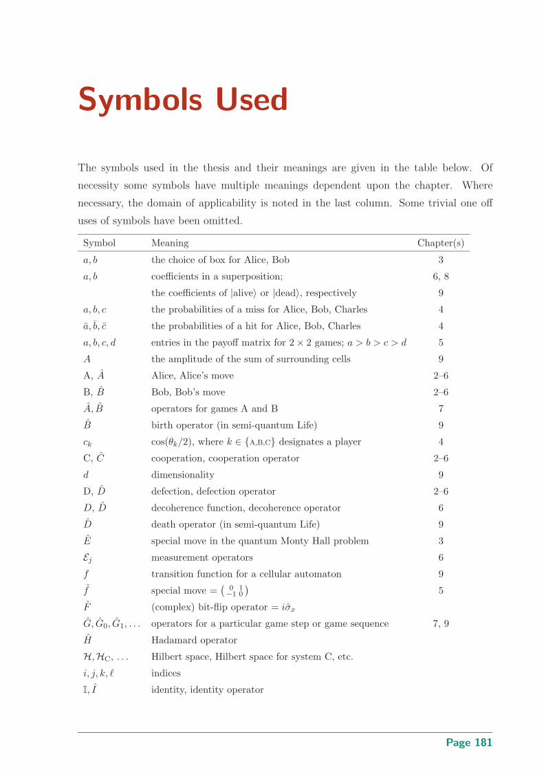
Symbols Used
The symbols used in the thesis and their meanings are given in the table below. Of
necessity some symbols have multiple meanings dependent upon the chapter. Where
necessary, the domain of applicability is noted in the last column. Some trivial one off
uses of symbols have been omitted.
Symbol Meaning Chapter(s)
a, b the choice of box for Alice, Bob 3
a, b coefficients in a superposition; 6, 8
the coefficients of |alive〉 or |dead〉, respectively 9
a, b, c the probabilities of a miss for Alice, Bob, Charles 4
a, b, c the probabilities of a hit for Alice, Bob, Charles 4
a, b, c, d entries in the payoff matrix for 2 × 2 games; a > b > c > d 5
A the amplitude of the sum of surrounding cells 9
A, A Alice, Alice’s move 2–6
B, B Bob, Bob’s move 2–6
A, B operators for games A and B 7
B birth operator (in semi-quantum Life) 9
ck cos(θk/2), where k ∈ A,B,C designates a player 4
C, C cooperation, cooperation operator 2–6
d dimensionality 9
D, D defection, defection operator 2–6
D, D decoherence function, decoherence operator 6
D death operator (in semi-quantum Life) 9
E special move in the quantum Monty Hall problem 3
Ej measurement operators 6
f transition function for a cellular automaton 9
f special move =(
0 1−1 0
)5
F (complex) bit-flip operator = iσx
G, G0, G1, . . . operators for a particular game step or game sequence 7, 9
H Hadamard operator
H,HC, . . . Hilbert space, Hilbert space for system C, etc.
i, j, k, ℓ indices
I, I identity, identity operator
Page 181
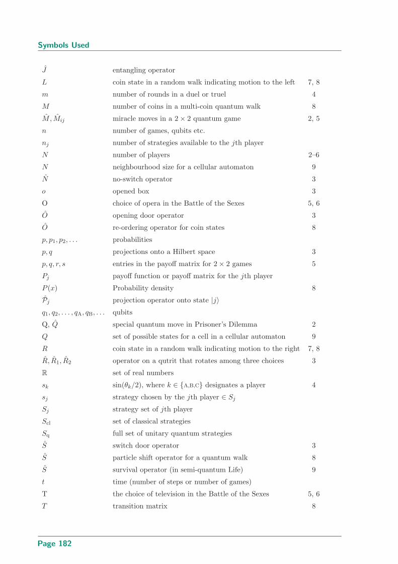
Symbols Used
J entangling operator
L coin state in a random walk indicating motion to the left 7, 8
m number of rounds in a duel or truel 4
M number of coins in a multi-coin quantum walk 8
M, Mij miracle moves in a 2 × 2 quantum game 2, 5
n number of games, qubits etc.
nj number of strategies available to the jth player
N number of players 2–6
N neighbourhood size for a cellular automaton 9
N no-switch operator 3
o opened box 3
O choice of opera in the Battle of the Sexes 5, 6
O opening door operator 3
O re-ordering operator for coin states 8
p, p1, p2, . . . probabilities
p, q projections onto a Hilbert space 3
p, q, r, s entries in the payoff matrix for 2 × 2 games 5
Pj payoff function or payoff matrix for the jth player
P (x) Probability density 8
Pj projection operator onto state |j〉q1, q2, . . . , qA, qB, . . . qubits
Q, Q special quantum move in Prisoner’s Dilemma 2
Q set of possible states for a cell in a cellular automaton 9
R coin state in a random walk indicating motion to the right 7, 8
R, R1, R2 operator on a qutrit that rotates among three choices 3
R set of real numbers
sk sin(θk/2), where k ∈ A,B,C designates a player 4
sj strategy chosen by the jth player ∈ Sj
Sj strategy set of jth player
Scl set of classical strategies
Sq full set of unitary quantum strategies
S switch door operator 3
S particle shift operator for a quantum walk 8
S survival operator (in semi-quantum Life) 9
t time (number of steps or number of games)
T the choice of television in the Battle of the Sexes 5, 6
T transition matrix 8
Page 182
Symbols Used
u2, u3 utility of survival in a pair or three-some in a truel 4
U unitary operator, generally ∈ SU(2)
Uj (unitary) move of player j
U unitary operator in (classical) subset of SU(2)
V special move =(
1 −11 1
)/√
2 5
VA(x), VB(x) potentials 7
x cos2(θA/2) cos2(θB/2) + sin2(θA/2) sin2(θA/2) 6
x position in a one-dimensional array of lattice sites 8, 9
y(t) vector representing the results at times t − 1 and t − 2 8
Z the set of integers
α superposition of the surrounding cells 9
α, β parameters in potentials 7
α, β, αj , βj phase factors (in an SU(2) operator)
γ entangling parameter 2, 4–6
γ controls the mix of switching or not-switching 3
Γ set of payoff functions = P1, . . . , PNǫ a small positive number, 0 < ǫ ≪ 1
θ, θj rotation angle (in an SU(2) operator)
πij , π, πs probability, probability vector, same for stationary state 8
ρ density matix 6
ρ, ρk, ρij , . . . coin probabilities in a history-dependent quantum walk 8
σx, σy, σz Pauli spin matrices
φ phase factor
ψ, ξ quantum system
Ω set of strategy sets = S1, . . . , SN$, $A, $B payoff, payoff to Alice, Bob
$ij payoff for the game result |ij〉$k
ξ payoff to the kth player for game result |ξ〉 6
$AAB etc. payoff for the sequence of games AAB etc. in a Parrondo game 7
Page 183

Page 184
Index
algorithm, quantum, 91, 94, 131
ancillary
bits, 14
qubits, 14
system, 25
Battle of the Sexes, 51, 60, 61, 62
with decoherence 72, 73
bit-flip opertor, 13
Brownian ratchet, 77, 78
cellular automata (CA), 106
1D nearest neighbour, 107
partitioned, 106, 107
quantum (QCA), 105, 108
quantum, 1D nearest neighbour, 109, 110
reversible, 106
Chicken, 51, 55–58, 62
with decoherence, 72, 73
coin toss, quantum, 83, 95
cooperation, 11, 50, 51
correlations
classical and quantum, 18
EPR, 20
counterstrategy, 16, 30
critical entanglement, 16, 53, 56, 62
Deadlock, 51, 57–59, 62
decoherence, 18, 47, 48, 65–75, 91, 103
decoherence free subspaces, 66
defection, 11, 50, 51
depasing, 66
duel, 33, 35
duel, quantum, 37, 38–41
econophysics, 21
Eisert’s scheme, 14–18, 50
with decoherence, 69, 70
entangling operator, 15, 52
error correction, quantum, 66
evolutionary stable strategy (ESS), 10, 18
extensive form, 10
flashing ratchet, 78
focal point, 9
Fokker-Planck equation, 92
game, 8
continuous variable, 20
incomplete information, 20
multiplayer, 19, 20, 61, 71
perfect information, 9
symmetric, 9, 11, 70
two person, 14
without entanglement, 20
zero sum, 9, 11
Hadamard operator, 12, 68, 83
Hilbert space, infinite dimensional, 75
initial state
maximally entangled, 29, 88
unentangled, 27
Life (game of), 106
birth, 111, 114
death, 111, 114
semi-quantum, 110–119
destructive interference, 117
structures, 118, 119
structures (classical), 109, 110
survival, 111, 114
Maple routines, 162–166
Marinatto and Weber’s scheme, 18
market games, quantum, 21
Markov chain, 101
Matching Pennies, 10
Mathematica routines, 137–162
maximin, 9, 39, 59
measurement, quantum, 13, 14, 25, 67
Page 185

Index
Minority game, 19
miracle move, 16, 50, 52
Monty Hall problem, 20, 23
classical, 24
quantum, 24–30
N -uels, quantum, 45
Nash equilibrium (NE), 9, 11, 17, 28, 30, 53, 55,
58, 59, 60
noise, 66
Markovian, 75
non-Markovian, 75
normal form, 10
operator sum representation, 66, 67
Pareto optimal (PO), 10, 11, 53, 55, 58, 59, 60
Parrondo games, 21, 77
classical, 79–82
capital-dependent, 79, 80
history-dependent, 79, 81, 82, 101
quantum, 82–92, 99
position-dependent, 82–86
history-dependent, 84, 87–91, 102
other, 91
payoff, 8, 15, 27, 33, 37, 69
Penny Flip, 12, 13
with decoherence, 68
potential, 83, 84
Prisoners’ Dilemma, 11, 51, 53, 54, 62
repeated, 18
three player, 19, 128
with decoherence, 71, 72
quantum algorithms, 91, 94
quantum coin, 83, 94
quantum computer, NMR, 17, 94
quantum walk, 93–103
biased multi-coin, 99, 100
diffusion of, 94
Hadamard, 95
history-dependent, multi-coin, 96–102
multi-coin, 97
single coin, 95
unbiased, multi-coin, 98
unbiased, single coin, 96
queuing, quantum, 125
qutrit, 25
Rock-Scissors-Paper, 20
Stag Hunt, 51, 58–60, 62
strategic form, 10
strategy, 8
classical, 13, 50, 70
dominant, 9, 11, 53, 58
mixed, 9, 11
mixed classical, 15
mixed quantum, 17, 30
pure, 9, 11
pure quantum, 50
three-parameter strategies, 16
truel, 31
classical 32–36
quantum, 36–46
quantum with decoherence, 47, 48
two-parameter strategies, 16
unitary strategies, 15
utility, 8
Page 186

Resume
Adrian Paul Flitney completed a Bachelor of Science with first class
honours in theoretical physics at the University of Tasmania in 1983. He was on the
Dean of Science roll of excellence in each undergraduate year. He worked in the field
of ionospheric physics and high frequency radio communication, for the Department of
Science in 1984–5 and for Andrew Antennas Corporation in 1988. During 1987–92 Flitney
was a researcher in quantum field theory at the Department of Physics and Mathematical
Physics, The University of Adelaide. During this period, and subsequently, he worked
as a tutor for the department and privately. In 2001 he began a PhD in the field of
quantum game theory at the Department of Electrical and Electronic Engineering, The
University of Adelaide under the supervision of Associate Professor Derek Abbott. He
has authored ten peer reviewed publications and has presented five conference papers,
including the ISDG best student paper at the 9th International Symposium on Dynamic
Games and Applications, Adelaide, 2000. He was awarded an Australian Research Council
(ARC) Postdoctoral Fellowship to study quantum games and decoherence at the School
of Physics, University of Melbourne for the period 2005–7.
Flitney’s non-academic interests include chess, where he was actively involved in admin-
istration for many years. He continues to be a regular competitor and has won a number
of events including four Tasmanian state titles.
Page 187